Geometric thermodynamics of reaction-diffusion systems: Thermodynamic trade-off relations and optimal transport for pattern formation

Abstract

The geometric approach to nonequilibrium thermodynamics is promising for understanding the role of dissipation and thermodynamic trade-off relations. This paper proposes a geometric framework for studying the nonequilibrium thermodynamics of reaction-diffusion systems. Based on this framework, we obtain several decompositions of the entropy production rate with respect to conservativeness, spatial structure, and wavenumber. We also generalize optimal transport theory to reaction-diffusion systems and derive several trade-off relations, including thermodynamic speed limits and thermodynamic uncertainty relations. The thermodynamic trade-off relations obtained in this paper shed light on thermodynamic dissipation in pattern formation. We numerically demonstrate our results using the Fisher–Kolmogorov–Petrovsky–Piskunov equation and the Brusselator model and discuss how the spatial pattern affects unavoidable dissipation.

I Introduction

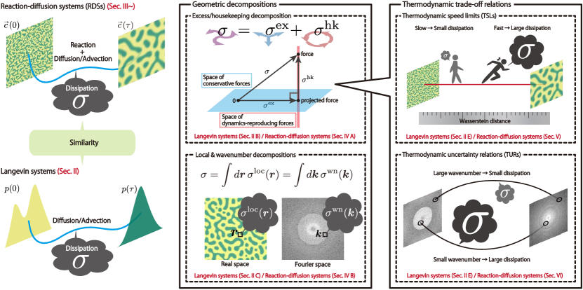
Figure 1: Schematics of the results in this paper. The red letters in the figure indicate the corresponding chapters. (Left panel) The similarity between RDSs and Langevin systems. For Langevin systems, we consider the time evolution from the probability $p(0)$ at time $t=0$ to the probability $p(\tau)$ at time $t=\tau$. For RDSs, we consider the time evolution from the concentration $\mathchoice{\kern-0.15pt\overset{\kern 0.7pt\smash{\lower 1.07639pt\hbox{\scalebox{0.45}{$\bm{\rightarrow}$}}}\kern-0.3pt}{c}}{\kern-0.15pt\overset{\kern 0.7pt\smash{\lower 1.07639pt\hbox{\scalebox{0.45}{$\bm{\rightarrow}$}}}\kern-0.3pt}{c}}{\overset{\smash{\lower 0.6458pt\hbox{\kern 0.2pt\scalebox{0.3}{$\bm{\rightarrow}$}\kern-0.8pt}}}{c}}{\overset{\smash{\lower 0.6458pt\hbox{\kern 0.2pt\scalebox{0.3}{$\bm{\rightarrow}$}\kern-0.8pt}}}{c}}(0)$ at time $t=0$ to the concentration $\mathchoice{\kern-0.15pt\overset{\kern 0.7pt\smash{\lower 1.07639pt\hbox{\scalebox{0.45}{$\bm{\rightarrow}$}}}\kern-0.3pt}{c}}{\kern-0.15pt\overset{\kern 0.7pt\smash{\lower 1.07639pt\hbox{\scalebox{0.45}{$\bm{\rightarrow}$}}}\kern-0.3pt}{c}}{\overset{\smash{\lower 0.6458pt\hbox{\kern 0.2pt\scalebox{0.3}{$\bm{\rightarrow}$}\kern-0.8pt}}}{c}}{\overset{\smash{\lower 0.6458pt\hbox{\kern 0.2pt\scalebox{0.3}{$\bm{\rightarrow}$}\kern-0.8pt}}}{c}}(\tau)$ at time $t=\tau$. Dissipation is quantified by the EPR $\sigma$ for the both systems. (Middle panel) Geometric decompositions of the EPR, the excess/housekeeping decomposition, the local decomposition and the wavenumber decomposition. The EPR $\sigma$ is decomposed into the excess EPR $\sigma^{\rm ex}$ and the housekeeping EPR $\sigma^{\rm hk}$, which corresponds to the contributions of the conservative force and the nonconservative force, respectively. This decomposition is introduced by projecting the force onto the space of conservative forces. The EPR $\sigma$ is also given by the integral of the local EPR $\sigma^{\rm loc}(\bm{r})$ in real space, and the integral of the wavenumber EPR $\sigma^{\rm wn}(\bm{k})$ in Fourier space. (Right panel) Thermodynamic trade-off relations, TSLs and TURs. TSLs refer to a trade-off between dissipation and speed. If the speed of the transition between initial and final states is slower, the dissipation can be smaller. The distance between initial and final states is measured by the Wasserstein distance and the minimal amount of dissipation also depends on this distance. TURs refer to the trade-off between dissipation and the change of the spatial pattern. More dissipation is required to change the mode corresponding to smaller wavenumbers.

Reaction-diffusion systems (RDSs) are used to study the formation of various spatiotemporal patterns, such as nanoscopic atomic patterns [1, 2], oscillatory phenomena in biochemical reactions [3, 4], morphological patterns in organisms [5, 6], and traveling waves in population dynamics [7]. Since the pioneering work of Turing [8], many studies have been conducted on the dynamical aspects of RDSs. For instance, analysis by reduction equations [9, 10] helps determine the stability of spatial patterns against perturbations and the time evolution of chemical waves.

The energetic understanding of pattern formations based on universal thermodynamic relations is still elusive. In order to discuss the energetic efficiency of pattern formation, it is necessary to quantify the relations between the complex dynamics of RDSs and the quantities that represent energy dissipation, such as entropy production (EP) and entropy production rate (EPR). Prigogine and his collaborators studied nonequilibrium thermodynamics of RDSs by assuming local equilibrium and paved the way to explore such relations [11, 12]. Many attempts, however, ended up with the calculation of concrete examples [13, 14, 15, 16] rather than laws that are universally valid for general RDSs. Recently, the thermodynamic structure of RDSs and simpler chemical reaction networks (CRNs) has been reorganized [17, 18, 19] following the development of stochastic thermodynamics of mesoscopic systems [20, 21]. It has led to active attempts to link dynamics and dissipation in RDSs (e.g., the relations between the speed of traveling waves that appear in RDSs and the dissipation [22], the thermodynamic constraints on certain classes of RDSs that conserve mass [23], and the dissipation in phase separation [24]). These are results for particular classes of RDSs, with results for general systems yet to be determined.

Stochastic thermodynamics provides methods to quantify the relation between dynamics and dissipation for mesoscopic systems. One approach is the decomposition of EPR. Decomposing EPR according to different sources lets us quantitatively understand where and how much dissipation occurs in the dynamics. One decomposition that has attracted particular attention is the decomposition into excess EPR, which becomes zero in steady state, and housekeeping EPR, which remains positive even in steady state [25]. Such decomposition is not unique: Besides the well-known Hatano–Sasa (or adiabatic/nonadiabatic) decomposition [26, 27], there is another decomposition proposed by Maes and Netočný for Langevin systems [28, 29, 30]. The other approach is the thermodynamic trade-off relations, which allow us to determine the minimum dissipation necessary to achieve specific goals. Two prime examples of such trade-off relations are the thermodynamic uncertainty relations (TURs), trade-off relations between precision and dissipation [31, 32], and the thermodynamic speed limits (TSLs), trade-off relations between speed and dissipation [33, 34, 35, 36, 37, 38, 39, 40, 41, 42, 43, 44, 45]. These two approaches, EPR decompositions and trade-off relations, are closely related in terms of geometry [35, 29, 40, 42].

A geometric theory called optimal transport theory, which deals with the transportation of probability distributions [46], plays an important role in stochastic thermodynamics. A fundamental quantity is the Wasserstein distance, which is a metric between two probability distributions and is used in various fields [47, 48, 49]. From a thermodynamic perspective, the Wasserstein distances determine minimum dissipation [50, 33, 34, 37, 38, 39, 40, 41] and have gained attention in various problems in thermodynamics, such as optimal control of thermal engines [51, 37, 52] and information thermodynamics [37, 53, 41, 54]. In particular, we can reinterpret the excess/housekeeping decomposition proposed by Maes and Netočný for Langevin systems from the perspective of optimal transport [29, 30, 40]. We can also obtain various TSLs by quantifying speed using the Wasserstein distances [33, 34, 36, 37, 38, 39, 40, 41, 42, 43, 44].

The methods developed in stochastic thermodynamics have been extended from stochastic to deterministic systems through geometric analogies. The decomposition proposed by Maes and Netočný has been reinterpreted from the perspective of the geometry of thermodynamic forces for Langevin systems [29, 30, 55], and extended to deterministic CRNs [40, 56, 42] and fluid systems [57]. Thermodynamic trade-off relations have also been extended to deterministic systems. The decomposition induces the TURs for deterministic CRNs [58, 40, 42]. In addition, generalizing Wasserstein distances leads to the TSLs for deterministic CRNs [40, 43]. These recent results for deterministic systems are based on the geometric structure of nonequilibrium thermodynamics, referred to as geometric thermodynamics [55].

Here we extend the framework of geometric thermodynamics to general RDSs, including RDSs driven by particle exchange with outside and external mechanical forces, and demonstrate connections between thermodynamic dissipation and pattern formation. We introduce two geometric decompositions of the EPR. One is decomposition into the excess part due to relaxation and the housekeeping part due to driving, which is a generalization of the decomposition for CRNs [40]. The other is decomposition into contributions occurring at each point in real or Fourier space. We also establish Wasserstein distances for RDSs by generalizing previous approaches [41, 59, 60, 61]. By relating such distances with the excess EPR, we obtain new TSLs for RDSs. We also obtain new TURs connecting the time variation of observables and dissipation for pattern formation in RDS. In particular, one of the TURs reveals that more dissipation is required to change the mode corresponding to smaller wavenumbers (lower spatial frequencies).

The paper is organized as follows (See also Fig. 1 for key results and the sections in which they appear). Starting from Langevin systems, we first explain the framework of geometric thermodynamics in Sec. II. This part is essentially an aid to understanding the main result for RDSs. We introduce the geometric excess/housekeeping decomposition of the EPR in Sec. II.2, the Wasserstein distances in Sec. II.4, and thermodynamic trade-off relations in Sec. II.5. Sec. II also contains a new result, the wavenumber decomposition of the EPR discussed in Sec. II.3. All subsequent sections are results for RDSs. In Sec. III, we explain thermodynamics of RDSs. We introduce vector notations of quantities, inner products, and generalizations of differential operators to simplify the description in Sec. III.4. We provide geometric decompositions of the EPR in Sec. IV. We discuss the excess/housekeeping decomposition in Sec. IV.1 and the local and wavenumber decompositions in Sec. IV.2. We generalize the Wasserstein distances and derive the TSLs in Sec. V. We also derive TURs in Sec. VI. In Sec. IV,  V, and  VI, at the end of each section, we demonstrate the results of that section using two simple systems, the Fisher–Kolmogorov–Petrovsky–Piskunov (Fisher–KPP) equation and the Brusselator model. In the Appendices, we present more mathematical details, derivations, and additional numerical examples. In particular, Appendix C considers the relationship between gradient flow, relaxation dynamics, and excess EPR, while Appendix E provides the detailed properties of generalized Wasserstein distances defined in Sec. V.

II Geometric thermodynamics for Langevin systems

Before discussing the results in RDSs, we briefly discuss geometric thermodynamics for Langevin systems [55]. We discuss the natural extension to RDSs later.

In the following, we consider a particle in Brownian motion in a $d$-dimensional Euclidean space $\mathbb{R}^{d}$. We assume the temperature is homogenous, and we set the temperature and Boltzmann’s constant to unity for simplicity. The following Langevin equation describes the time evolution of the position of the Brownian particle,

$$d_{t}\check{\bm{r}}(t)=-D\bm{\nabla}_{\bm{r}}U(\check{\bm{r}}(t);t)+D\bm{K}^{\rm nc}(\check{\bm{r}}(t);t)+\sqrt{2D}\bm{\xi}(t),$$ (1)

where $d_{t}=d/dt$ stands for the time derivative, $\check{\bm{r}}(t)$ indicates the position of the Brownian particle at time $t$, $\bm{\nabla}_{\bm{r}}$ is the differential operator for spatial coordinates $\bm{r}\in\mathbb{R}^{d}$, $-\bm{\nabla}_{\bm{r}}U(\check{\bm{r}}(t);t)\coloneqq-\left.\bm{\nabla}_{\bm{r}}U(\bm{r};t)\right|_{\bm{r}=\check{\bm{r}}(t)}$ indicates the potential force on the particle, $\bm{K}^{\rm nc}(\check{\bm{r}}(t);t)$ indicates the nonconservative mechanical force on the particle, $D$ is the diffusion constant which is given by the mobility and temperature, and $\bm{\xi}(t)=(\xi_{i}(t))_{i=1}^{d}$ is the white Gaussian noise satisfying $\langle\xi_{i}(t)\rangle=0$ and $\langle\xi_{i}(t)\xi_{j}(t^{\prime})\rangle=\delta_{ij}\delta(t-t^{\prime})$. In later sections, we will use some of the symbols introduced in this section to represent their counterparts in RDSs.

II.1 Fokker–Planck equation and entropy production rate

The probability density $p(\bm{r};t)$ of the Brownian particle at position $\bm{r}$ at time $t$ described by the Langevin equation Eq. (1) evolves according to the Fokker–Planck equation,

$$\partial_{t}p(\bm{r};t)=-\bm{\nabla}_{\bm{r}}\cdot\bm{J}(\bm{r};t),$$ (2)

$$\bm{J}(\bm{r};t)\coloneqq Dp(\bm{r};t)\quantity[-\bm{\nabla}_{\bm{r}}(U(\bm{r};t)+\ln p(\bm{r};t))+\bm{K}^{\rm nc}(\bm{r};t)],$$ (3)

where $\partial_{t}=\partial/\partial t$ stands for the partial time derivative and $\bm{J}(\bm{r};t)$ is the thermodynamic current. Here, $p(\bm{r};t)$ is the probability density, and thus $\int_{\mathbb{R}^{d}}d\bm{r}p(\bm{r};t)=1$ and $p(\bm{r};t)\geq 0$ hold. In the following, we assume boundary conditions, $p(\bm{r};t)$ and its derivatives vanish as $\|\bm{r}\|\to\infty$, where $\|\cdot\|$ is the Euclidean norm.

Defining thermodynamic force $\bm{F}(\bm{r};t)$ as

$$\bm{F}(\bm{r};t)\coloneqq-\bm{\nabla}_{\bm{r}}(U(\bm{r};t)+\ln p(\bm{r};t))+\bm{K}^{\rm nc}(\bm{r};t),$$ (4)

the thermodynamic current $\bm{J}$ and force $\bm{F}$ satisfy a linear relation,

$$\bm{J}(\bm{r};t)=\mathsf{M}(\bm{r};t)\bm{F}(\bm{r};t),$$ (5)

where the $d\times d$ positive-definite matrix $\mathsf{M}_{ij}(\bm{r};t)\coloneqq Dp(\bm{r};t)\delta_{ij}$ indicates the mobility tensor. We can rewrite the Fokker–Planck equation in Eq. (2) as $\partial_{t}p=-\bm{\nabla}_{\bm{r}}\cdot\quantity(\mathsf{M}\bm{F})$.

The EPR $\sigma$ for Langevin systems is written as an inner product of $\bm{J}$ and $\bm{F}$ or a square norm of $\bm{F}$,

$$\sigma \coloneqq\left\llangle\bm{J},\bm{F}\right\rrangle=\left\llangle\mathsf{M}\bm{F},\bm{F}\right\rrangle=\left\llangle\bm{F},\bm{F}\right\rrangle_{\mathsf{M}}$$

$$=\int_{\mathbb{R}^{d}}d\bm{r}Dp(\bm{r};t)\|\bm{F}(\bm{r};t)\|^{2},$$ (6)

where the inner products $\left\llangle\cdot,\cdot\right\rrangle$ and $\left\llangle\cdot,\cdot\right\rrangle_{\mathsf{M}}$ are defined as $\left\llangle\bm{J}^{\prime},\bm{F}^{\prime}\right\rrangle\coloneqq\int_{\mathbb{R}^{d}}d\bm{r}\bm{J}^{\prime}(\bm{r})\cdot\bm{F}^{\prime}(\bm{r})$ and $\left\llangle\bm{F}^{\prime},\bm{F}^{\prime\prime}\right\rrangle_{\mathsf{M}}\coloneqq\left\llangle\mathsf{M}\bm{F}^{\prime},\bm{F}^{\prime\prime}\right\rrangle$ for all vector-valued functions $\bm{J}^{\prime}(\bm{r})$, $\bm{F}^{\prime}(\bm{r})$ and $\bm{F}^{\prime\prime}(\bm{r})$ that take values at $\mathbb{R}^{d}$. The mobility tensor $\mathsf{M}$ may be regarded as the metric tensor because $\mathsf{M}$ is positive-definite. We also introduce the EP $\Sigma_{\tau}$ as $\Sigma_{\tau}\coloneqq\int_{0}^{\tau}dt\,\sigma_{t}$, where $\sigma_{t}$ denotes the EPR at time $t$.

II.2 Geometric excess/housekeeping decomposition of entropy production rate for Langevin systems

The Langevin system in Eq. (1) is driven by two contributions: one is the conservative contribution, which causes relaxation to the equilibrium state corresponding to $U(\bm{r};t)$, and the other is the nonconservative contribution due to $\bm{K}^{\mathrm{nc}}(\bm{r};t)$, which keeps the system out of equilibrium even in the steady state. The thermodynamic force $\bm{F}$ in Eq. (4) contains the two contributions, the conservative force $-\bm{\nabla}_{\bm{r}}(U(\bm{r};t)+\ln p(\bm{r};t))$, which is the gradient of the quantity $-(U(\bm{r};t)+\ln p(\bm{r};t))$, and the nonconservative force $\bm{K}^{\mathrm{nc}}$. Thus, the EPR $\sigma=\left\llangle\bm{F},\bm{F}\right\rrangle_{\mathsf{M}}$ quantifies these two contributions simultaneously.

To quantify the conservative and nonconservative contributions separately, we construct the geometric decomposition of the EPR by utilizing the generalized Pythagorean theorem for the force space with the inner product $\left\llangle,\right\rrangle_{\mathsf{M}}$:

$$\left\llangle\bm{F},\bm{F}\right\rrangle_{\mathsf{M}}=\left\llangle\bm{F}^{\ast},\bm{F}^{\ast}\right\rrangle_{\mathsf{M}}+\left\llangle\bm{F}-\bm{F}^{\ast},\bm{F}-\bm{F}^{\ast}\right\rrangle_{\mathsf{M}},$$ (7)

which is valid when we decompose $\bm{F}$ into two orthogonal parts $\bm{F}^{\ast}$ and $\bm{F}-\bm{F}^{\ast}$, satisfying

$$\left\llangle\bm{F}^{\ast},\bm{F}-\bm{F}^{\ast}\right\rrangle_{\mathsf{M}}=0.$$ (8)

The force $\bm{F}^{\ast}$ which allows for the Pythagorean theorem [Eq. (7)] is not unique [30]. We focus on $\bm{F}^{\ast}$ which enables us to regard $\left\llangle\bm{F}^{\ast},\bm{F}^{\ast}\right\rrangle_{\mathsf{M}}$ and $\left\llangle\bm{F}-\bm{F}^{\ast},\bm{F}-\bm{F}^{\ast}\right\rrangle_{\mathsf{M}}$ as the dissipation due to conservative and nonconservative forces, respectively. For this purpose, we assume $\bm{F}^{\ast}(\bm{r};t)$ is the gradient of a potential as $\bm{F}^{\ast}(\bm{r};t)=\bm{\nabla}_{\bm{r}}\phi^{\ast}(\bm{r};t)$, inspired by the original form of the conservative force $-\bm{\nabla}_{\bm{r}}(U(\bm{r};t)+\ln p(\bm{r};t))$. Then, we can derive the condition on $\phi^{\ast}$ as the sufficient condition for the orthogonality in Eq. (8),

$$\bm{\nabla}_{\bm{r}}\cdot\quantity(\mathsf{M}\bm{\nabla}_{\bm{r}}\phi^{\ast})=\bm{\nabla}_{\bm{r}}\cdot\quantity(\mathsf{M}\bm{F}),$$ (9)

which let us determine $\bm{F}^{\ast}$ uniquely (see Appendix A.1 for details).

Using the decomposition of the force $\bm{F}$ into conservative part $\bm{F}^{\ast}$ and its orthogonal part $\bm{F}-\bm{F}^{\ast}$, we define the excess and the housekeeping EPRs as $\sigma^{\mathrm{ex}}\coloneqq\left\llangle\bm{F}^{\ast},\bm{F}^{\ast}\right\rrangle_{\mathsf{M}}$ and $\sigma^{\mathrm{hk}}\coloneqq\left\llangle\bm{F}-\bm{F}^{\ast},\bm{F}-\bm{F}^{\ast}\right\rrangle_{\mathsf{M}}$, respectively. These EPRs are nonnegative because they are represented by the squared norm. Then, the Pythagorean theorem [Eq. (7)] is a decomposition of EPR into the excess and the housekeeping EPRs,

$$\sigma=\sigma^{\mathrm{ex}}+\sigma^{\mathrm{hk}}.$$ (10)

Time integration gives a decomposition of the EP $\Sigma_{\tau}$ into the excess EP $\Sigma_{\tau}^{\mathrm{ex}}$ and the housekeeping EP $\Sigma_{\tau}^{\mathrm{hk}}$,

$$\Sigma_{\tau}=\Sigma^{\mathrm{ex}}_{\tau}+\Sigma^{\mathrm{hk}}_{\tau}.$$ (11)

Here, the excess EP $\Sigma_{\tau}^{\mathrm{ex}}$ and the housekeeping EP $\Sigma_{\tau}^{\mathrm{hk}}$ are defined as

$$\Sigma_{\tau}^{\mathrm{ex}}\coloneqq\int_{0}^{\tau}dt\sigma^{\mathrm{ex}}_{t},\;\;\Sigma_{\tau}^{\mathrm{hk}}\coloneqq\int_{0}^{\tau}dt\sigma^{\mathrm{hk}}_{t},$$ (12)

where $\sigma^{\mathrm{ex}}_{t}$ is the excess EPR at time $t$ and $\sigma^{\mathrm{hk}}_{t}$ is the housekeeping EPR at time $t$.

Since the geometric decomposition [Eq. (10)] is a generalized Pythagorean theorem, we can conceptualize the decomposition geometrically, as summarized in Fig. 2. Firstly, let us consider the geometric nature of the excess EPR. The conservative force $\bm{F}^{\ast}=\bm{\nabla}_{\bm{r}}\phi^{\ast}$, whose squared norm provides the excess EPR, is uniquely given by the minimization problem

$$\bm{F}^{\ast}=\operatorname*{arg\,min}_{\bm{F}^{\prime}|\bm{\nabla}_{\bm{r}}\cdot\quantity(\mathsf{M}\bm{F}^{\prime})=\bm{\nabla}_{\bm{r}}\cdot\quantity(\mathsf{M}\bm{F})}\left\llangle\bm{F}^{\prime},\bm{F}^{\prime}\right\rrangle_{\mathsf{M}},$$ (13)

which follows from condition Eq. (9) (see Appendix A.2 for details). As a result, we can rewrite the excess EPR $\sigma^{\mathrm{ex}}$ as the following variational problem

$$\sigma^{\mathrm{ex}}=\inf_{\bm{F}^{\prime}|\bm{\nabla}_{\bm{r}}\cdot\quantity(\mathsf{M}\bm{F}^{\prime})=\bm{\nabla}_{\bm{r}}\cdot\quantity(\mathsf{M}\bm{F})}\left\llangle\bm{F}^{\prime},\bm{F}^{\prime}\right\rrangle_{\mathsf{M}}.$$ (14)

The minimization problem [Eq. (13)] means that $\bm{F}^{*}$ is the closest point to the origin $\bm{0}$ in the affine subspace $\{\bm{F}^{\prime}\mid\bm{\nabla}_{\bm{r}}\cdot[\mathsf{M}(\bm{F}-\bm{F}^{\prime})]=0\}$. The excess EPR can be seen as the shortest distance between this affine subspace and the origin.

We can also obtain a geometric interpretation of the housekeeping EPR because the set of conservative forces is the image of the gradient operator $\mathrm{Im}\,\bm{\nabla}_{\bm{r}}\coloneqq\quantity{\bm{F}^{\prime}\mid\exists\phi,\;\bm{F}^{\prime}=\bm{\nabla}_{\bm{r}}\phi}$, and $\bm{F}-\bm{F}^{\prime}$ for the element $\bm{F}^{\prime}\in\{\bm{F}^{\prime}\mid\bm{\nabla}_{\bm{r}}\cdot[\mathsf{M}(\bm{F}-\bm{F}^{\prime})]=0\}$ is in the orthogonal complement of $\mathrm{Im}\,\bm{\nabla}_{\bm{r}}$ with respect to the inner product $\left\llangle\cdot,\cdot\right\rrangle_{\mathsf{M}}$. Consequently, the geometric decomposition [Eq. (10)] can also be treated from the viewpoint of the projection onto the subspace $\mathrm{Im}\bm{\nabla}_{\bm{r}}$: the conservative force $\bm{F}^{\ast}$ is given by the minimization problem

$$\bm{F}^{\ast}=\operatorname*{arg\,min}_{\bm{F}^{\prime}\in\mathrm{Im}\bm{\nabla}_{\bm{r}}}\left\llangle\bm{F}-\bm{F}^{\prime},\bm{F}-\bm{F}^{\prime}\right\rrangle_{\mathsf{M}}.$$ (15)

This is derived similarly to Eq. (13) by using the condition in Eq. (9) (see Appendix A.2 for details). Then, we can rewrite the housekeeping EPR $\sigma^{\mathrm{hk}}$ as the variational problem

$$\sigma^{\mathrm{hk}}=\inf_{\phi}\left\llangle\bm{F}-\bm{\nabla}_{\bm{r}}\phi,\bm{F}-\bm{\nabla}_{\bm{r}}\phi\right\rrangle_{\mathsf{M}},$$ (16)

which shows that the housekeeping EPR is the squared distance between the actual force and the subspace of the conservative forces.

In addition to the geometric interpretations, the constraint in Eq. (14) lets us discuss the physical meanings of the decomposition. The constraint with the Fokker–Planck equation $\partial_{t}p(\bm{r};t)=-\bm{\nabla}_{\bm{r}}\cdot(\mathsf{M}\bm{F})$ yields the relation

$$\partial_{t}p=-\bm{\nabla}_{\bm{r}}\cdot\quantity(\mathsf{M}\bm{F}^{\ast}),$$ (17)

so we can interpret the excess EPR as the minimum dissipation required to reproduce the original dynamics. In contrast, the housekeeping EPR reflects the dissipation caused by the cyclic current that does not affect the dynamics, because $\bm{J}^{\mathrm{hk}}\coloneqq\mathsf{M}\quantity(\bm{F}-\bm{\nabla}_{\bm{r}}\phi^{\ast})$ satisfies $\bm{\nabla}_{\bm{r}}\cdot\bm{J}^{\mathrm{hk}}=0$.

If the nonconservative force $\bm{K}^{\mathrm{nc}}$ in Eq. (4) is absent, then the housekeeping EPR always vanishes, and the optimal potential $\phi^{\ast}$ is given by $\phi^{\ast}=-U-\ln p$. Conversely, the excess EPR vanishes when the system is in steady state since the condition in Eq. (9) reduces to $\bm{\nabla}_{\bm{r}}\cdot(\mathsf{M}\bm{F}^{\ast})=0$ in steady state, which $\bm{F}^{\ast}=\bm{0}$ solves.

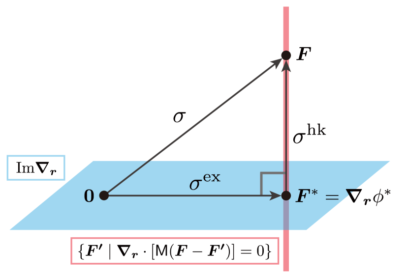
Figure 2: The geometric decomposition of the EPR for Langevin systems. The blue plane indicates $\mathrm{Im}\bm{\nabla}_{\bm{r}}$, and the red line indicates $\{\bm{F}^{\prime}|\bm{\nabla}_{\bm{r}}\cdot[\mathsf{M}(\bm{F}-\bm{F}^{\prime})]=0\}$. The thermodynamic force, whose squared norm is the EPR as $\sigma=\left\llangle\bm{F},\bm{F}\right\rrangle_{\mathsf{M}}$, is decomposed into the two orthogonal parts: $\bm{F}^{\ast}$ is the projection of $\bm{F}$ onto $\mathrm{Im}\bm{\nabla}_{\bm{r}}$, whose squared norm is the excess EPR as $\sigma^{\mathrm{ex}}=\left\llangle\bm{F^{\ast}},\bm{F^{\ast}}\right\rrangle_{\mathsf{M}}$, and the remaining part $\bm{F}-\bm{F}^{\ast}$, whose squared norm is the housekeeping EPR as $\sigma^{\mathrm{hk}}=\left\llangle\bm{F}-\bm{F^{\ast}},\bm{F}-\bm{F^{\ast}}\right\rrangle_{\mathsf{M}}$. We can regard $\bm{F}^{\ast}$ as the projection of $\bm{0}$ onto the red line or of $\bm{F}$ onto the blue plane.

II.3 Local decomposition and wavenumber decomposition of entropy production rate for Langevin systems

The EPR is the volume integral of the positive quantity $\bm{J}(\bm{r};t)\cdot\bm{F}(\bm{r};t)$. From this viewpoint, we can decompose the dissipation at each spatial location. Similarly, it is expected that we can identify the dissipation at each wavenumber in the Fourier space. In this section, we introduce two new kinds of geometric decompositions of the EPR. One is a decomposition of the EPR into contributions from each spatial location, and the other is a decomposition into contributions from each wavenumber.

Local decomposition— Firstly, we define the local EPR as

$$\sigma_{t}^{\mathrm{loc}}(\bm{r})\coloneqq\bm{J}(\bm{r};t)\cdot\bm{F}(\bm{r};t)\geq 0,$$ (18)

which satisfies

$$\sigma_{t}=\int_{\mathbb{R}^{d}}d\bm{r}\,\sigma_{t}^{\mathrm{loc}}(\bm{r}).$$ (19)

The local EPR $\sigma_{t}^{\mathrm{loc}}(\bm{r})$ is nonnegative and indicates dissipation at location $\bm{r}$.

We can also decompose the excess and housekeeping EPRs as $\sigma_{t}^{\mathrm{ex}}=\int_{\mathbb{R}^{d}}d\bm{r}\sigma_{t}^{\mathrm{ex,loc}}(\bm{r})$, and $\sigma_{t}^{\mathrm{hk}}=\int_{\mathbb{R}^{d}}d\bm{r}\sigma_{t}^{\mathrm{hk,loc}}(\bm{r})$, where the local excess and housekeeping EPRs are defined as

$$\sigma_{t}^{\mathrm{ex,loc}}(\bm{r}) \coloneqq\bm{\nabla}_{\bm{r}}\phi^{\ast}(\bm{r};t)\cdot\mathsf{M}(\bm{r};t)\bm{\nabla}_{\bm{r}}\phi^{\ast}(\bm{r};t)$$

$$=\bm{F}^{\ast}(\bm{r};t)\cdot\mathsf{M}(\bm{r};t)\bm{F}^{\ast}(\bm{r};t),$$ (20)

and

$$\sigma_{t}^{\mathrm{hk,loc}}(\bm{r})\coloneqq[ \bm{F}(\bm{r};t)-\bm{\nabla}_{\bm{r}}\phi^{\ast}(\bm{r};t)]$$

$$\cdot\mathsf{M}(\bm{r};t)[\bm{F}(\bm{r};t)-\bm{\nabla}_{\bm{r}}\phi^{\ast}(\bm{r};t)].$$ (21)

The local excess and housekeeping EPRs are nonnegative because the mobility tensor $\mathsf{M}$ is positive-definite for all $\bm{r}\in V$. Note that $\phi^{\ast}$ is a solution of the partial differential equation in Eq. (9), which means that we need global information to obtain the local excess and housekeeping EPRs.

Because these local excess and housekeeping EPRs are not introduced by the geometric decomposition for the local EPR $\sigma_{t}^{\mathrm{loc}}$, the geometric excess/housekeeping decomposition can be locally violated as

$$\sigma_{t}^{\mathrm{loc}}(\bm{r})\neq\sigma_{t}^{\mathrm{ex,loc}}(\bm{r})+\sigma_{t}^{\mathrm{hk,loc}}(\bm{r}).$$ (22)

In other words, there may be a non-zero cross-term,

$$\sigma_{t}^{\mathrm{cross}}(\bm{r}) \coloneqq\sigma_{t}^{\mathrm{loc}}(\bm{r})-\sigma_{t}^{\mathrm{ex,loc}}(\bm{r})-\sigma_{t}^{\mathrm{hk,loc}}(\bm{r})$$

$$=2\bm{\nabla}_{\bm{r}}\phi^{\ast}\cdot\mathsf{M}[\bm{F}-\bm{\nabla}_{\bm{r}}\phi^{\ast}].$$ (23)

The cross-term may be negative or positive, but it satisfies $\int_{\mathbb{R}^{d}}d\bm{r}\,\sigma_{t}^{\mathrm{cross}}(\bm{r})=0$, thereby guaranteeing that the geometric excess/housekeeping decomposition holds globally as $\sigma_{t}=\sigma_{t}^{\mathrm{ex}}+\sigma_{t}^{\mathrm{hk}}$.

Wavenumber decomposition— Next, we decompose the EPR into nonnegative wavenumber components using Parseval’s identity. Because Parseval’s identity can be regarded as a generalization of the Pythagorean theorem, we can regard this decomposition as another kind of geometric decomposition. We define the wavenumber EPR as

$$\sigma_{t}^{\mathrm{wn}}(\bm{k})\coloneqq\frac{1}{(2\pi)^{d}}\|\hat{\bm{F}}(\bm{k};t)\|^{2}\geq 0,$$ (24)

where we introduced the weighted Fourier transform of a vector field $\bm{F}^{\prime}$ with a weight $\sqrt{\mathsf{M}_{ii}}=\sqrt{Dp(\bm{r};t)}$ defined as

$$\hat{F}^{\prime}_{i}(\bm{k};t)\coloneqq\int_{\mathbb{R}^{d}}d\bm{r}\sqrt{Dp(\bm{r};t)}F^{\prime}_{i}(\bm{r};t)\mathrm{e}^{-\mathrm{i}\bm{k}\cdot\bm{r}}.$$ (25)

Note that $\hat{\bm{F}}(\bm{k};t)$ is a complex vector and its Euclidean norm is defined as $\|\hat{\bm{F}}\|\coloneqq\sqrt{\sum_{i=1}^{d}\overline{\hat{F}_{i}}\hat{F}_{i}}$ with the overline indicating complex conjugate. The wavenumber EPR $\sigma_{t}^{\mathrm{wn}}(\bm{k})$ provides a decomposition of EPR as

$$\sigma_{t}=\int_{\mathbb{R}^{d}}d\bm{k}\,\sigma_{t}^{\mathrm{wn}}(\bm{k}).$$ (26)

Though this can be understood as a consequence of Parseval’s identity, we can show it directly as

$$\int_{\mathbb{R}^{d}}d\bm{k}\,\sigma_{t}^{\mathrm{wn}}(\bm{k})=\frac{1}{(2\pi)^{d}}\int_{\mathbb{R}^{d}}d\bm{k}\|\hat{\bm{F}}(\bm{k};t)\|^{2}.$$

$$\quad=\int_{\mathbb{R}^{d}\times\mathbb{R}^{d}}d\bm{r}d\bm{r}^{\prime}\left[\left\{\frac{1}{(2\pi)^{d}}\int_{\mathbb{R}^{d}}d\bm{k}\mathrm{e}^{\mathrm{i}\bm{k}\cdot(\bm{r}-\bm{r}^{\prime})}\right\}\right.$$

$$\quad\left.\phantom{\int_{\mathbb{R}^{d}}d\bm{k}}\times D\sqrt{p(\bm{r};t)p(\bm{r}^{\prime};t)}\bm{F}(\bm{r};t)\cdot\bm{F}^{\prime}(\bm{r}^{\prime};t)\right]$$

$$\quad=\int_{\mathbb{R}^{d}}d\bm{r}Dp(\bm{r};t)\|\bm{F}(\bm{r};t)\|^{2}=\sigma_{t}.$$ (27)

Here, we use the Fourier transform of the delta function $\delta(\bm{r}-\bm{r}^{\prime})=\int_{\mathbb{R}^{d}}d\bm{k}\mathrm{e}^{\mathrm{i}\bm{k}\cdot(\bm{r}-\bm{r}^{\prime})}/(2\pi)^{d}$.

As we did for local EPR, we can also decompose the excess and housekeeping EPRs into wavenumber contributions as $\sigma_{t}^{\mathrm{ex}}=\int_{\mathbb{R}^{d}}d\bm{k}\,\sigma_{t}^{\mathrm{ex,wn}}(\bm{k})$, and $\sigma_{t}^{\mathrm{hk}}=\int_{\mathbb{R}^{d}}d\bm{k}\,\sigma_{t}^{\mathrm{hk,wn}}(\bm{k})$ by defining the wavenumber excess and housekeeping EPRs as

$$\sigma_{t}^{\mathrm{ex,wn}}(\bm{k})\coloneqq\frac{1}{(2\pi)^{d}}\|\hat{F}^{\ast}(\bm{k};t)\|^{2},$$ (28)

and

$$\sigma_{t}^{\mathrm{hk,wn}}(\bm{k})\coloneqq\frac{1}{(2\pi)^{d}}\|\hat{F}(\bm{k};t)-\hat{F}^{\ast}(\bm{k};t)\|^{2}.$$ (29)

We remark that the geometric excess/housekeeping decomposition can also be violated at each wavenumber as $\sigma_{t}^{\mathrm{wn}}(\bm{k})\neq\sigma_{t}^{\mathrm{ex,wn}}(\bm{k})+\sigma_{t}^{\mathrm{hk,wn}}(\bm{k})$, and there is a nonzero cross term $\sigma_{t}^{\mathrm{cross,wn}}(\bm{k})\coloneqq\sigma_{t}^{\mathrm{wn}}(\bm{k})-\sigma_{t}^{\mathrm{ex,wn}}(\bm{k})+\sigma_{t}^{\mathrm{hk,wn}}(\bm{k})$ which satisfies $\int_{\mathbb{R}^{d}}d\bm{k}\sigma_{t}^{\mathrm{cross,wn}}(\bm{k})=0$.

The wavenumber decomposition is based on the orthonormality of the Fourier basis. Therefore, it may be possible to generalize the geometric decomposition of the EPR using an orthonormal basis other than the Fourier basis, e.g., a wavelet basis [62, 63]. It may also be interesting to consider the spectral decomposition of the EPR [64] based on the Harada–Sasa relation [65] in terms of our wavenumber decomposition.

II.4 Wasserstein distance

The excess EPR obtained in the previous section can be interpreted as a geometric quantity using the Wasserstein geometry developed in optimal transport theory [46, 30]. Here, we briefly review the Wasserstein distance and its dynamical reformulation, which is intrinsically important in thermodynamics.

The $q$-Wasserstein distance for a positive number $q\geq 1$ between two probability distributions $p_{A}$ and $p_{B}$ is defined as

$${W}_{q}(p_{A},p_{B})\coloneqq$$

$$\left(\inf_{\pi\in\Pi(p_{A},p_{B})}\int_{\mathbb{R}^{d}\times\mathbb{R}^{d}}d\bm{r}d\bm{r^{\prime}}\|\bm{r}-\bm{r}^{\prime}\|^{q}\pi(\bm{r},\bm{r}^{\prime})\right)^{\frac{1}{q}},$$ (30)

where $\Pi(p_{A},p_{B})$ is the set of joint probability distributions with marginals $p_{A}$ and $p_{B}$:

$$\Pi(p_{A},p_{B})\coloneqq \left\{\pi\middle|\;p_{A}(\bm{r})=\int_{\mathbb{R}^{d}}d\bm{r}^{\prime}\pi(\bm{r},\bm{r}^{\prime}),\right.$$

$$\left.p_{B}(\bm{r}^{\prime})=\int_{\mathbb{R}^{d}}d\bm{r}\pi(\bm{r},\bm{r}^{\prime}),\;\pi(\bm{r},\bm{r}^{\prime})\geq 0\right\}.$$

Here we assume that the moments up to the $q$-th order are finite for the two probability distributions $p_{A}$ and $p_{B}$. We can confirm that ${W}_{q}$ indeed satisfies the axioms of distance. We can also prove

$${W}_{q}(p_{A},p_{B})\leq{W}_{q^{\prime}}(p_{A},p_{B})\;\;\mathrm{for}\;\;q\leq q^{\prime},$$ (31)

by Hölder’s inequality [46].

For every $q$, we can reformulate the $q$-Wasserstein distance as an optimization problem related to the dynamics of a probability distribution subject to a continuity equation. In particular, we can obtain the square of the $2$-Wasserstein distance by the minimization problem

$${W}_{2}(p_{A},p_{B})^{2}=\inf_{p,\bm{F}^{\prime}}\tau\int_{0}^{\tau}dt\int_{\mathbb{R}^{d}}d\bm{r}\|D\bm{F}^{\prime}(\bm{r};t)\|^{2}p(\bm{r};t)$$ (32)

with the following three constraints

$$p(\cdot;0)=p_{A}(\cdot),\;p(\cdot;\tau)=p_{B}(\cdot),\;\partial_{t}p=-\bm{\nabla}_{\bm{r}}\cdot\quantity(pD\bm{F}^{\prime}).$$ (33)

In other words, we minimize the right-hand side in Eq. (32) over trajectories of probability distributions that start and end on $p_{A}$ and $p_{B}$ and satisfy a continuity equation. This reformulation for the case $q=2$ was initially made by Benamou and Brenier, so the equation (32) is called Benamou–Brenier formula in optimal transport theory [50]. We also can consider an extension of the Benamou–Brenier formula for general $q$ [66, 67, 68]. Especially in the case of $q=1$, we can express the Benamou–Brenier formula as optimization of the current instead of the force,

$${W}_{1}(p_{A},p_{B})=\inf_{p,\bm{J}^{\prime}}\int_{0}^{\tau}dt\int_{\mathbb{R}^{d}}d\bm{r}\|\bm{J}^{\prime}(\bm{r};t)\|$$ (34)

with the constraints

$$p(\cdot;0)=p_{A}(\cdot),\;p(\cdot;\tau)=p_{B}(\cdot),\;\partial_{t}p=-\bm{\nabla}_{\bm{r}}\cdot\bm{J}^{\prime}.$$ (35)

Both expressions of $1$-Wasserstein distance in the original definition [Eq. (II.4)] and the Benamou–Brenier formula [Eq. (34)] are reduced to an expression known as Kantorovich–Rubinstein duality,

$${W}_{1}(p_{A},p_{B})=\sup_{\phi\in\mathrm{Lip}^{1}}\quantity{\int_{\mathbb{R}^{d}}d\bm{r}\phi\quantity(p_{B}-p_{A})},$$ (36)

where the set of $1$-Lipschitz functions is denoted by

$$\mathrm{Lip}^{1}\coloneqq\quantity{\phi\mid\|\bm{\nabla}_{\bm{r}}\phi\|\leq 1}.$$ (37)

The derivation of Eq. (36) from the original definition of the $1$-Wasserstein distance in Eq. (II.4) is well-known and based on the method of Lagrange multipliers [46]. The Benamou–Brenier formula [Eq. (34)] can be directly obtained from Kantorovich–Rubinstein duality [Eq. (36)] by again using the method of Lagrange multipliers [69].

II.5 Wasserstein geometry and thermodynamic trade-off relations

Considering a trajectory of probability distribution $\left\{p(t)\right\}_{t\in[0,\tau]}$ obeying the Fokker–Planck equation [Eq. (2)], we can define the length of the trajectory using the $q$-Wasserstein distance as

$$l_{q,\tau}\coloneqq\int_{0}^{\tau}dt\,v_{q}(t)\,,$$ (38)

with $v_{q}(t)$ defined as

$$v_{q}(t)\coloneqq\lim_{\varDelta t\to 0}\frac{{W}_{q}\quantity(p(t),p(t+\varDelta t))}{\varDelta t}.$$ (39)

This quantity $v_{q}(t)$ indicates the speed of the dynamics of $p(t)$ on the space of probability distributions. The form of the mobility tensor $\mathsf{M}$, the Benamou–Brenier formula for the $2$-Wasserstein distance [Eq. (32)], and the variational form of the excess EPR [Eq. (14)] lead to

$$\sigma_{t}^{\mathrm{ex}}=\frac{v_{2}(t)^{2}}{D},$$ (40)

which means the square root of the excess EPR is proportional to the speed of the dynamics of the probability distribution.

The relation between $\sigma_{t}^{\mathrm{ex}}$ and $v_{2}(t)$ leads to the hierarchy of TSLs [37]

$$\frac{{W}_{2}(p(0),p(\tau))^{2}}{D}\leq\frac{l_{2,\tau}^{2}}{D}\leq\tau\Sigma^{\mathrm{ex}}_{\tau}\leq\tau\Sigma_{\tau}.$$ (41)

Inequality $l_{2,\tau}\geq{W}_{2}(p(0),p(\tau))$, which comes from the triangle inequality, yields the first inequality in Eq. (41). This inequality reflects the fact that ${W}_{2}(p(0),p(\tau))$ is the length of the geodesic connecting $p(0)$ and $p(\tau)$. The second inequality is derived from the Cauchy–Schwarz inequality $\left[\int_{0}^{\tau}dtv_{2}(t)\right]^{2}\leq\left[\int_{0}^{\tau}dt\right]\left[\int_{0}^{\tau}dtv_{2}(t)^{2}\right]$ and the relation between $v_{2}$ and $\sigma^{\mathrm{ex}}$ [Eq. (40)]. The third inequality is a consequence of the nonnegativity of the housekeeping EP $\Sigma^{\mathrm{hk}}_{\tau}\geq 0$ and Eq. (11). Overall, the inequalities in Eq. (41) tell us that transitioning to a more distant distribution in less time requires more dissipation.

The inequality between Wasserstein distances in Eq. (31) leads to another hierarchy of TSLs as

$$\frac{{W}_{1}(p(0),p(\tau))^{2}}{D}\leq\frac{l_{1,\tau}^{2}}{D}\leq\tau\Sigma^{\mathrm{ex}}_{\tau}\leq\tau\Sigma_{\tau}.$$ (42)

These lower bounds on the EPs are weaker than those in Eq. (41) because Eq. (31) shows

$$\frac{l_{1,\tau}^{2}}{D} \leq\frac{l_{2,\tau}^{2}}{D}\leq\tau\Sigma_{\tau},$$

$$\frac{{W}_{1}(p(0),p(\tau))^{2}}{D} \leq\frac{{W}_{2}(p(0),p(\tau))^{2}}{D}\leq\tau\Sigma_{\tau},$$ (43)

where we used the fact that Eq. (31) leads to $v_{2}(t)\geq v_{1}(t)$ and $l_{2,\tau}\geq l_{1,\tau}$. The generalization of the TLSs discussed here from Langevin dynamics to Markov jump processes (MJPs) is rather complicated, and we only note that there are multiple ways of generalizing [40, 41].

Using the excess EPR, we can obtain a TUR for time-independent observable $\varphi(\bm{r})$ as

$$(d_{t}\langle\varphi\rangle_{p_{t}})^{2}\leq D\left\langle\|\bm{\nabla}_{\bm{r}}\varphi\|^{2}\right\rangle_{p_{t}}\sigma^{\mathrm{ex}}_{t},$$ (44)

where the bracket indicates the average over the probability distribution $p(\bm{r};t)$, $\langle\varphi\rangle_{p_{t}}\coloneqq\int_{\mathbb{R}^{d}}d\bm{r}p(\bm{r};t)\varphi(\bm{r})$ [29]. The TUR represents a trade-off relation between the dissipation, $\sigma^{\mathrm{ex}}_{t}$, the speed of the observable, $d_{t}\langle\varphi\rangle_{p_{t}}$, and average squared magnitude of the gradient of the observable, $\left\langle\|\bm{\nabla}_{\bm{r}}\varphi\|^{2}\right\rangle_{p_{t}}$. In other words, we need more dissipation to make a flatter observable change faster. It is derived from the Cauchy–Schwarz inequality, $\left\llangle\bm{\nabla}_{\bm{r}}\varphi,\bm{\nabla}_{\bm{r}}\phi^{\ast}\right\rrangle^{2}_{\mathsf{M}}\leq\left\llangle\bm{\nabla}_{\bm{r}}\varphi,\bm{\nabla}_{\bm{r}}\varphi\right\rrangle_{\mathsf{M}}\left\llangle\bm{\nabla}_{\bm{r}}\phi^{\ast},\bm{\nabla}_{\bm{r}}\phi^{\ast}\right\rrangle_{\mathsf{M}}$, and the fact that $\phi^{\ast}$ reproduces the dynamics as $\partial_{t}p=-\bm{\nabla}_{\bm{r}}\cdot(\mathsf{M}\bm{\nabla}_{\bm{r}}\phi^{\ast})$. Here, the quantities appearing in the Cauchy–Schwarz inequality are given by $\left\llangle\bm{\nabla}_{\bm{r}}\varphi,\bm{\nabla}_{\bm{r}}\phi^{\ast}\right\rrangle_{\mathsf{M}}=d_{t}\langle\varphi\rangle_{p_{t}}$, $\left\llangle\bm{\nabla}_{\bm{r}}\varphi,\bm{\nabla}_{\bm{r}}\varphi\right\rrangle_{\mathsf{M}}=D\left\langle\|\bm{\nabla}_{\bm{r}}\varphi\|^{2}\right\rangle_{p_{t}}$ and $\left\llangle\bm{\nabla}_{\bm{r}}\phi^{\ast},\bm{\nabla}_{\bm{r}}\phi^{\ast}\right\rrangle_{\mathsf{M}}=\sigma^{\mathrm{ex}}_{t}$, which proves the TUR.

We can also interpret the TUR from the viewpoint of the Wasserstein geometry by rewriting Eq. (44) as

$$v_{\varphi}(t)\coloneqq\frac{|d_{t}\langle\varphi\rangle_{p_{t}}|}{\sqrt{\left\langle\|\bm{\nabla}_{\bm{r}}\varphi\|^{2}\right\rangle_{p_{t}}}}\leq v_{2}(t),$$ (45)

using the relation between $v_{2}(t)$ and $\sigma^{\mathrm{ex}}_{t}$ in Eq. (40). Here, we define $v_{\varphi}(t)$ as the speed of the observable $\varphi$ normalized by the spatial fluctuation of $\varphi$. Therefore, the TUR means that the normalized speed of an observable is slower than the speed of the probability distribution moving on the manifold of distributions equipped with the Wasserstein metric. This is similar to the Cramér–Rao bound [70] with parameter $t$, called the information geometric speed limit [71, 72], written as

$$v_{\varphi}^{I}(t)\coloneqq\frac{|d_{t}\langle\varphi\rangle_{p_{t}}|}{\sqrt{\mathrm{Var}[\varphi]}}\leq v_{I}(t),$$ (46)

where $v_{I}(t)\coloneqq\sqrt{\langle(d_{t}\ln p(t))^{2}\rangle_{p_{t}}}$ is the square root of the Fisher information and $\mathrm{Var}[\varphi]$ is the variance defined as $\mathrm{Var}[\varphi]=\langle\varphi^{2}\rangle_{p_{t}}-\langle\varphi\rangle^{2}_{p_{t}}$. From the viewpoint of information geometry, we can regard $v_{I}(t)$ as the speed of the probability distribution, $p(t)$, on the manifold equipped with the information-geometric (Fisher) metric.

We can derive the inequality $v_{1}(t)\leq v_{2}(t)$, which provides the hierarchy of TSLs [Eq. (II.5)], from the TUR by taking the optimal potential of the Kantorovich–Rubinstein duality [Eq. (36)] as the observable in Eq. (45).

III Thermodynamics of reaction-diffusion systems

Hereafter, we will focus on reaction-diffusion systems (RDSs). We will refer to the geometric framework reviewed above, while also introducing new notions to generalize it. We will need to use many kinds of symbols, which we summarize in Table. 1.

This section introduces the basics of RDSs, dynamics and thermodynamics. We begin with one class of RDSs called closed systems in Sec. III.1. A closed RDS does not exchange molecules with the outside, as opposed to an open RDS, the other class of RDSs as explained in Sec. III.2. Section III.3 introduces the thermodynamics of RDSs in terms of thermodynamic forces and the EPR. To simplify the discussion in subsequent sections, we unify quantities associated with reaction and diffusion by introducing appropriate vector fields and operators in Sec. III.4. We also introduce the concept of the conservative and nonconservative thermodynamic forces for RDSs, which play a central role in the geometric excess/housekeeping decomposition of EPR in Sec. III.5.

III.1 Closed reaction-diffusion systems

We consider an RDS describing the time evolution of a concentration distribution of $N$ chemical species in $d$-dimensional area $V\subseteq\mathbb{R}^{d}$ due to reactions, advection, and diffusion. If no particles interact with the outside of the system, the system is called a closed RDS. Let $\mathcal{S}$ index the chemical species as $\mathcal{S}\coloneqq\quantity{1,2,\cdots,N}$. We denote the $\alpha$-th chemical species ($\alpha\in\mathcal{S}$) as $Z_{\alpha}$, and its concentration distribution at location $\bm{r}\in V$ and time $t$ as $c_{\alpha}(\bm{r};t)$. We remark that $c_{\alpha}(\bm{r};t)$ is not a probability density and $\int d\bm{r}c_{\alpha}(\bm{r};t)$ is not necessarily equal to $1$ or any other constant.

Usually, the dynamics of the concentration of $\alpha$-th chemical species under the assumption of Fick’s law are given by the reaction-diffusion (RD) equation,

$$\partial_{t}c_{\alpha}(\bm{r};t)=D_{\alpha}\bm{\nabla}_{\bm{r}}^{2}c_{\alpha}(\bm{r};t)+R_{\alpha}(\bm{r};t),$$ (47)

where $D_{\alpha}$ indicates the diffusion constant of $Z_{\alpha}$ and $R_{\alpha}(\bm{r};t)$ represents the effect of reactions. Note that the reaction term $R_{\alpha}$ can depend on the concentration distribution. We can rewrite the first term to $-\bm{\nabla}_{\bm{r}}\cdot\bm{J}_{(\alpha)}^{\mathrm{Fick}}(\bm{r};t)$, where $\bm{J}_{(\alpha)}^{\mathrm{Fick}}(\bm{r};t)\coloneqq-D_{\alpha}\bm{\nabla}_{\bm{r}}c_{\alpha}(\bm{r};t)$ is the current obeying Fick’s law.

Assuming Fick’s law is optional to our discussion. The diffusion current given by Fick’s law sometimes fails to describe the dynamics of chemical species, for example, under an electric field, which causes advection, or in a non-dilute solution. To include a wider range of phenomena, we deal with the following more general equation for $\alpha$-th chemical species,

$$\partial_{t}c_{\alpha}(\bm{r};t)=-\bm{\nabla}_{\bm{r}}\cdot\bm{J}_{(\alpha)}(\bm{r};t)+R_{\alpha}(\bm{r};t),$$ (48)

where $\bm{J}_{(\alpha)}(\bm{r};t)=[J_{(\alpha)i}(\bm{r};t)]_{i=1,\cdots,d}$ is the general diffusion current for $\alpha$-th species. If $\bm{J}_{(\alpha)}(\bm{r};t)=\bm{J}_{(\alpha)}^{\mathrm{Fick}}(\bm{r};t)$, Eq. (48) reproduces Eq. (47). The diffusion currents can depend on the concentration distribution.

We assume one of the following three boundary conditions on diffusion currents in this paper. Note that the boundary conditions on diffusion currents constrain concentration distributions through the dependence of diffusion currents on the concentration distributions. The first one is the no-flux boundary condition, $\bm{J}_{(\alpha)}(\bm{r};t)\cdot\bm{n}(\bm{r})=0$ for all $\alpha\in\mathcal{S}$, $t$, and $\bm{r}\in\partial V$, where $\partial V$ indicates the boundary of $V$, and $\bm{n}(\bm{r})$ is the unit normal vector of the surface at $\bm{r}\in\partial V$. This condition corresponds to considering a chemical reaction system in a container, where the exchange of particles via diffusion with the outside never happens. The second one is the periodic boundary condition: when the space $V$ has a periodic structure, like a supercube, we may assume that all quantities depending on $\bm{r}$ satisfy the periodic boundary condition. Note that this rule applies not only to the currents but also to the other quantities. The third one is the fast decay of the diffusion currents at infinity, which we consider when $V=\mathbb{R}^{d}$. Those conditions can be combined. For example, considering an infinitely long pipe with a square cross-section, we may assume the no-flux boundary or the periodic boundary on the sides of the pipe, while supposing the fast decay for the current at infinity.

We can consider the thermodynamic structure of the RDS by rewriting the reaction term $R_{\alpha}(\bm{r};t)$ with reaction currents based on the details of reactions, as explained below. We consider $M$ reactions indexed by $\mathcal{R}\coloneqq\quantity{1,2,\cdots,M}$. We write $\rho$-th reaction ($\rho\in\mathcal{R}$) as

$$\ce{$\sum_{\alpha\in\mathcal{S}}\nu_{\alpha\rho}^{+}Z_{\alpha}$<=>$\sum_{\alpha\in\mathcal{S}}\nu_{\alpha\rho}^{-}Z_{\alpha}$}$$

where $\nu_{\alpha\rho}^{\pm}$ indicates the number of $Z_{\alpha}$ consumed ($+$) or produced ($-$) by $\rho$-th reaction. We assume $\nu_{\alpha\rho}^{\pm}$ is independent of location $\bm{r}$ and time $t$ for all $\alpha$ and $\rho$. We write the forward ($+$) and the reverse ($-$) flux of the $\rho$-th reaction at $(\bm{r};t)$ as $j^{+}_{\rho}(\bm{r};t)$ and $j^{-}_{\rho}(\bm{r};t)$, respectively. All the fluxes are always assumed to be positive $j^{\pm}_{\rho}(\bm{r};t)>0$. They can depend on space and time $(\bm{r};t)$ directly and/or via concentration distributions (e.g., assuming mass-action kinetics, a flux is given by $j^{\pm}_{\rho}(\bm{r};t)=k_{\rho}^{\pm}(\bm{r};t)\prod_{\alpha}\quantity[c_{\alpha}(\bm{r};t)]^{\nu_{\alpha\rho}^{\pm}}$, where $k_{\rho}^{\pm}(\bm{r};t)$ is the reaction rate constant for the positive/reverse reaction). The reaction current of $\rho$-th reaction $j_{\rho}(\bm{r};t)$ is given by $j_{\rho}(\bm{r};t)=j_{\rho}^{+}(\bm{r};t)-j_{\rho}^{-}(\bm{r};t)$. Using these reaction currents, we can rewrite $R_{\alpha}(\bm{r};t)$ as

$$R_{\alpha}(\bm{r};t)=\sum_{\rho\in\mathcal{R}}S_{\alpha\rho}j_{\rho}(\bm{r};t),$$ (49)

where $S_{\alpha\rho}\coloneqq\nu_{\alpha\rho}^{-}-\nu_{\alpha\rho}^{+}$ is the $(\alpha,\rho)$-th element of the stoichiometric matrix, which denotes the net increase of $Z_{\alpha}$ through the $\rho$-th reaction.

To simplify the notation, we sometimes make the dependence on $(\bm{r};t)$ implicit as

$$\partial_{t}c_{\alpha} =-\bm{\nabla}_{\bm{r}}\cdot\bm{J}_{(\alpha)}+R_{\alpha},$$ (50)

$$R_{\alpha} =\sum_{\rho\in\mathcal{R}}S_{\alpha\rho}j_{\rho}.$$ (51)

We further make it simpler by expressing $\alpha$ dependence with vector notation as

$$\partial_{t}\mathchoice{\kern-0.15pt\overset{\kern 0.7pt\smash{\lower 1.07639pt\hbox{\scalebox{0.45}{$\bm{\rightarrow}$}}}\kern-0.3pt}{c}}{\kern-0.15pt\overset{\kern 0.7pt\smash{\lower 1.07639pt\hbox{\scalebox{0.45}{$\bm{\rightarrow}$}}}\kern-0.3pt}{c}}{\overset{\smash{\lower 0.6458pt\hbox{\kern 0.2pt\scalebox{0.3}{$\bm{\rightarrow}$}\kern-0.8pt}}}{c}}{\overset{\smash{\lower 0.6458pt\hbox{\kern 0.2pt\scalebox{0.3}{$\bm{\rightarrow}$}\kern-0.8pt}}}{c}}=-\bm{\nabla}_{\bm{r}}\cdot\mathchoice{\kern-0.15pt\overset{\kern 0.7pt\smash{\lower 1.07639pt\hbox{\scalebox{0.45}{$\bm{\rightarrow}$}}}\kern-0.3pt}{\bm{J}}}{\kern-0.15pt\overset{\kern 0.7pt\smash{\lower 1.07639pt\hbox{\scalebox{0.45}{$\bm{\rightarrow}$}}}\kern-0.3pt}{\bm{J}}}{\overset{\smash{\lower 0.6458pt\hbox{\kern 0.2pt\scalebox{0.3}{$\bm{\rightarrow}$}\kern-0.8pt}}}{\bm{J}}}{\overset{\smash{\lower 0.6458pt\hbox{\kern 0.2pt\scalebox{0.3}{$\bm{\rightarrow}$}\kern-0.8pt}}}{\bm{J}}}+\mathchoice{\kern-0.15pt\overset{\kern 0.7pt\smash{\lower 1.07639pt\hbox{\scalebox{0.45}{$\bm{\rightarrow}$}}}\kern-0.3pt}{R}}{\kern-0.15pt\overset{\kern 0.7pt\smash{\lower 1.07639pt\hbox{\scalebox{0.45}{$\bm{\rightarrow}$}}}\kern-0.3pt}{R}}{\overset{\smash{\lower 0.6458pt\hbox{\kern 0.2pt\scalebox{0.3}{$\bm{\rightarrow}$}\kern-0.8pt}}}{R}}{\overset{\smash{\lower 0.6458pt\hbox{\kern 0.2pt\scalebox{0.3}{$\bm{\rightarrow}$}\kern-0.8pt}}}{R}}$$ (52)

where $\mathchoice{\kern-0.15pt\overset{\kern 0.7pt\smash{\lower 1.07639pt\hbox{\scalebox{0.45}{$\bm{\rightarrow}$}}}\kern-0.3pt}{c}}{\kern-0.15pt\overset{\kern 0.7pt\smash{\lower 1.07639pt\hbox{\scalebox{0.45}{$\bm{\rightarrow}$}}}\kern-0.3pt}{c}}{\overset{\smash{\lower 0.6458pt\hbox{\kern 0.2pt\scalebox{0.3}{$\bm{\rightarrow}$}\kern-0.8pt}}}{c}}{\overset{\smash{\lower 0.6458pt\hbox{\kern 0.2pt\scalebox{0.3}{$\bm{\rightarrow}$}\kern-0.8pt}}}{c}}=({c}_{1},\dots,{c}_{N}){}^{\top}$, $\mathchoice{\kern-0.15pt\overset{\kern 0.7pt\smash{\lower 1.07639pt\hbox{\scalebox{0.45}{$\bm{\rightarrow}$}}}\kern-0.3pt}{\bm{J}}}{\kern-0.15pt\overset{\kern 0.7pt\smash{\lower 1.07639pt\hbox{\scalebox{0.45}{$\bm{\rightarrow}$}}}\kern-0.3pt}{\bm{J}}}{\overset{\smash{\lower 0.6458pt\hbox{\kern 0.2pt\scalebox{0.3}{$\bm{\rightarrow}$}\kern-0.8pt}}}{\bm{J}}}{\overset{\smash{\lower 0.6458pt\hbox{\kern 0.2pt\scalebox{0.3}{$\bm{\rightarrow}$}\kern-0.8pt}}}{\bm{J}}}=(\bm{J}_{(1)},\dots,\bm{J}_{(N)}){}^{\top}$, $\mathchoice{\kern-0.15pt\overset{\kern 0.7pt\smash{\lower 1.07639pt\hbox{\scalebox{0.45}{$\bm{\rightarrow}$}}}\kern-0.3pt}{R}}{\kern-0.15pt\overset{\kern 0.7pt\smash{\lower 1.07639pt\hbox{\scalebox{0.45}{$\bm{\rightarrow}$}}}\kern-0.3pt}{R}}{\overset{\smash{\lower 0.6458pt\hbox{\kern 0.2pt\scalebox{0.3}{$\bm{\rightarrow}$}\kern-0.8pt}}}{R}}{\overset{\smash{\lower 0.6458pt\hbox{\kern 0.2pt\scalebox{0.3}{$\bm{\rightarrow}$}\kern-0.8pt}}}{R}}=(R_{1},\dots,R_{N}){}^{\top}$, and ^⊤ indicates transposition. We also define an $M\times N$ matrix $\nabla_{\mathsf{s}}$ as $(\nabla_{\mathsf{s}})_{\rho\alpha}\coloneqq S_{\alpha\rho}$, so that its transpose $\nabla_{\mathsf{s}}^{\top}$ is the stoichiometric matrix. By introducing a vector of reaction currents $\bm{j}=(j_{1},\dots,j_{M}){}^{\top}$, we can rewrite the reaction term as $\mathchoice{\kern-0.15pt\overset{\kern 0.7pt\smash{\lower 1.07639pt\hbox{\scalebox{0.45}{$\bm{\rightarrow}$}}}\kern-0.3pt}{R}}{\kern-0.15pt\overset{\kern 0.7pt\smash{\lower 1.07639pt\hbox{\scalebox{0.45}{$\bm{\rightarrow}$}}}\kern-0.3pt}{R}}{\overset{\smash{\lower 0.6458pt\hbox{\kern 0.2pt\scalebox{0.3}{$\bm{\rightarrow}$}\kern-0.8pt}}}{R}}{\overset{\smash{\lower 0.6458pt\hbox{\kern 0.2pt\scalebox{0.3}{$\bm{\rightarrow}$}\kern-0.8pt}}}{R}}=\nabla_{\mathsf{s}}^{\top}\bm{j}$ and the dynamics of a closed RDS as

$$\partial_{t}\mathchoice{\kern-0.15pt\overset{\kern 0.7pt\smash{\lower 1.07639pt\hbox{\scalebox{0.45}{$\bm{\rightarrow}$}}}\kern-0.3pt}{c}}{\kern-0.15pt\overset{\kern 0.7pt\smash{\lower 1.07639pt\hbox{\scalebox{0.45}{$\bm{\rightarrow}$}}}\kern-0.3pt}{c}}{\overset{\smash{\lower 0.6458pt\hbox{\kern 0.2pt\scalebox{0.3}{$\bm{\rightarrow}$}\kern-0.8pt}}}{c}}{\overset{\smash{\lower 0.6458pt\hbox{\kern 0.2pt\scalebox{0.3}{$\bm{\rightarrow}$}\kern-0.8pt}}}{c}}=-\bm{\nabla}_{\bm{r}}\cdot\mathchoice{\kern-0.15pt\overset{\kern 0.7pt\smash{\lower 1.07639pt\hbox{\scalebox{0.45}{$\bm{\rightarrow}$}}}\kern-0.3pt}{\bm{J}}}{\kern-0.15pt\overset{\kern 0.7pt\smash{\lower 1.07639pt\hbox{\scalebox{0.45}{$\bm{\rightarrow}$}}}\kern-0.3pt}{\bm{J}}}{\overset{\smash{\lower 0.6458pt\hbox{\kern 0.2pt\scalebox{0.3}{$\bm{\rightarrow}$}\kern-0.8pt}}}{\bm{J}}}{\overset{\smash{\lower 0.6458pt\hbox{\kern 0.2pt\scalebox{0.3}{$\bm{\rightarrow}$}\kern-0.8pt}}}{\bm{J}}}+\nabla_{\mathsf{s}}^{\top}\bm{j}.$$ (53)

There are two ways of writing a vector: $\bm{x}$ or $\mathchoice{\kern-0.15pt\overset{\kern 0.7pt\smash{\lower 1.07639pt\hbox{\scalebox{0.45}{$\bm{\rightarrow}$}}}\kern-0.3pt}{x}}{\kern-0.15pt\overset{\kern 0.7pt\smash{\lower 1.07639pt\hbox{\scalebox{0.45}{$\bm{\rightarrow}$}}}\kern-0.3pt}{x}}{\overset{\smash{\lower 0.6458pt\hbox{\kern 0.2pt\scalebox{0.3}{$\bm{\rightarrow}$}\kern-0.8pt}}}{x}}{\overset{\smash{\lower 0.6458pt\hbox{\kern 0.2pt\scalebox{0.3}{$\bm{\rightarrow}$}\kern-0.8pt}}}{x}}$. The former is always used for $d$-dimensional vectors, except for $\bm{j}$ which denotes the $M$-dimensional vector of reactions. The latter is always used to indicate an $N$-dimensional vector of a quantity defined for each species $\alpha$. For example, $\mathchoice{\kern-0.15pt\overset{\kern 0.7pt\smash{\lower 1.07639pt\hbox{\scalebox{0.45}{$\bm{\rightarrow}$}}}\kern-0.3pt}{\bm{J}}}{\kern-0.15pt\overset{\kern 0.7pt\smash{\lower 1.07639pt\hbox{\scalebox{0.45}{$\bm{\rightarrow}$}}}\kern-0.3pt}{\bm{J}}}{\overset{\smash{\lower 0.6458pt\hbox{\kern 0.2pt\scalebox{0.3}{$\bm{\rightarrow}$}\kern-0.8pt}}}{\bm{J}}}{\overset{\smash{\lower 0.6458pt\hbox{\kern 0.2pt\scalebox{0.3}{$\bm{\rightarrow}$}\kern-0.8pt}}}{\bm{J}}}$ has $N$ elements $\bm{J}_{(\alpha)}$ for each species $\alpha$, where $\bm{J}_{(\alpha)}$ is the $d$-dimensional vector representing the diffusion current of $Z_{\alpha}$.

III.2 Open reaction-diffusion systems

We generally deal with an open RDS, where some of the $N$ species can be exchanged with the outside of the system. We classify the species into two categories, internal species, which are not exchanged with the outside, and external species, which are exchanged with the outside. Let $N_{\mathcal{X}}(\leq N)$ denote the number of internal species. We index the internal and external species as $\mathcal{X}\coloneqq\quantity{1,\dots,N_{\mathcal{X}}}$ and $\mathcal{Y}\coloneqq\quantity{N_{\mathcal{X}}+1,\dots,N}=\mathcal{S}\setminus\mathcal{X}$, respectively.

Corresponding to the decomposition of $\mathcal{S}$ into $\mathcal{X}$ and $\mathcal{Y}$, we introduce the following notation. Let $\mathchoice{\kern-0.15pt\overset{\kern 0.7pt\smash{\lower 1.07639pt\hbox{\scalebox{0.45}{$\bm{\rightarrow}$}}}\kern-0.3pt}{e}}{\kern-0.15pt\overset{\kern 0.7pt\smash{\lower 1.07639pt\hbox{\scalebox{0.45}{$\bm{\rightarrow}$}}}\kern-0.3pt}{e}}{\overset{\smash{\lower 0.6458pt\hbox{\kern 0.2pt\scalebox{0.3}{$\bm{\rightarrow}$}\kern-0.8pt}}}{e}}{\overset{\smash{\lower 0.6458pt\hbox{\kern 0.2pt\scalebox{0.3}{$\bm{\rightarrow}$}\kern-0.8pt}}}{e}}=(e_{1},\cdots,e_{N}){}^{\top}$ be an arbitrary vector consisting of $N$ elements, like $\mathchoice{\kern-0.15pt\overset{\kern 0.7pt\smash{\lower 1.07639pt\hbox{\scalebox{0.45}{$\bm{\rightarrow}$}}}\kern-0.3pt}{c}}{\kern-0.15pt\overset{\kern 0.7pt\smash{\lower 1.07639pt\hbox{\scalebox{0.45}{$\bm{\rightarrow}$}}}\kern-0.3pt}{c}}{\overset{\smash{\lower 0.6458pt\hbox{\kern 0.2pt\scalebox{0.3}{$\bm{\rightarrow}$}\kern-0.8pt}}}{c}}{\overset{\smash{\lower 0.6458pt\hbox{\kern 0.2pt\scalebox{0.3}{$\bm{\rightarrow}$}\kern-0.8pt}}}{c}}$, $\mathchoice{\kern-0.15pt\overset{\kern 0.7pt\smash{\lower 1.07639pt\hbox{\scalebox{0.45}{$\bm{\rightarrow}$}}}\kern-0.3pt}{\bm{J}}}{\kern-0.15pt\overset{\kern 0.7pt\smash{\lower 1.07639pt\hbox{\scalebox{0.45}{$\bm{\rightarrow}$}}}\kern-0.3pt}{\bm{J}}}{\overset{\smash{\lower 0.6458pt\hbox{\kern 0.2pt\scalebox{0.3}{$\bm{\rightarrow}$}\kern-0.8pt}}}{\bm{J}}}{\overset{\smash{\lower 0.6458pt\hbox{\kern 0.2pt\scalebox{0.3}{$\bm{\rightarrow}$}\kern-0.8pt}}}{\bm{J}}}$ or $\mathchoice{\kern-0.15pt\overset{\kern 0.7pt\smash{\lower 1.07639pt\hbox{\scalebox{0.45}{$\bm{\rightarrow}$}}}\kern-0.3pt}{R}}{\kern-0.15pt\overset{\kern 0.7pt\smash{\lower 1.07639pt\hbox{\scalebox{0.45}{$\bm{\rightarrow}$}}}\kern-0.3pt}{R}}{\overset{\smash{\lower 0.6458pt\hbox{\kern 0.2pt\scalebox{0.3}{$\bm{\rightarrow}$}\kern-0.8pt}}}{R}}{\overset{\smash{\lower 0.6458pt\hbox{\kern 0.2pt\scalebox{0.3}{$\bm{\rightarrow}$}\kern-0.8pt}}}{R}}$. We define $\mathchoice{\kern-0.15pt\overset{\kern 0.7pt\smash{\lower 1.07639pt\hbox{\scalebox{0.45}{$\bm{\rightarrow}$}}}\kern-0.3pt}{e}}{\kern-0.15pt\overset{\kern 0.7pt\smash{\lower 1.07639pt\hbox{\scalebox{0.45}{$\bm{\rightarrow}$}}}\kern-0.3pt}{e}}{\overset{\smash{\lower 0.6458pt\hbox{\kern 0.2pt\scalebox{0.3}{$\bm{\rightarrow}$}\kern-0.8pt}}}{e}}{\overset{\smash{\lower 0.6458pt\hbox{\kern 0.2pt\scalebox{0.3}{$\bm{\rightarrow}$}\kern-0.8pt}}}{e}}_{\mathcal{X}}$ and $\mathchoice{\kern-0.15pt\overset{\kern 0.7pt\smash{\lower 1.07639pt\hbox{\scalebox{0.45}{$\bm{\rightarrow}$}}}\kern-0.3pt}{e}}{\kern-0.15pt\overset{\kern 0.7pt\smash{\lower 1.07639pt\hbox{\scalebox{0.45}{$\bm{\rightarrow}$}}}\kern-0.3pt}{e}}{\overset{\smash{\lower 0.6458pt\hbox{\kern 0.2pt\scalebox{0.3}{$\bm{\rightarrow}$}\kern-0.8pt}}}{e}}{\overset{\smash{\lower 0.6458pt\hbox{\kern 0.2pt\scalebox{0.3}{$\bm{\rightarrow}$}\kern-0.8pt}}}{e}}_{\mathcal{Y}}$ as the vectors of the first $N_{\mathcal{X}}$ elements and the last $N-N_{\mathcal{X}}$ elements of $\mathchoice{\kern-0.15pt\overset{\kern 0.7pt\smash{\lower 1.07639pt\hbox{\scalebox{0.45}{$\bm{\rightarrow}$}}}\kern-0.3pt}{e}}{\kern-0.15pt\overset{\kern 0.7pt\smash{\lower 1.07639pt\hbox{\scalebox{0.45}{$\bm{\rightarrow}$}}}\kern-0.3pt}{e}}{\overset{\smash{\lower 0.6458pt\hbox{\kern 0.2pt\scalebox{0.3}{$\bm{\rightarrow}$}\kern-0.8pt}}}{e}}{\overset{\smash{\lower 0.6458pt\hbox{\kern 0.2pt\scalebox{0.3}{$\bm{\rightarrow}$}\kern-0.8pt}}}{e}}$; thus, they decompose $\mathchoice{\kern-0.15pt\overset{\kern 0.7pt\smash{\lower 1.07639pt\hbox{\scalebox{0.45}{$\bm{\rightarrow}$}}}\kern-0.3pt}{e}}{\kern-0.15pt\overset{\kern 0.7pt\smash{\lower 1.07639pt\hbox{\scalebox{0.45}{$\bm{\rightarrow}$}}}\kern-0.3pt}{e}}{\overset{\smash{\lower 0.6458pt\hbox{\kern 0.2pt\scalebox{0.3}{$\bm{\rightarrow}$}\kern-0.8pt}}}{e}}{\overset{\smash{\lower 0.6458pt\hbox{\kern 0.2pt\scalebox{0.3}{$\bm{\rightarrow}$}\kern-0.8pt}}}{e}}$ as $\mathchoice{\kern-0.15pt\overset{\kern 0.7pt\smash{\lower 1.07639pt\hbox{\scalebox{0.45}{$\bm{\rightarrow}$}}}\kern-0.3pt}{e}}{\kern-0.15pt\overset{\kern 0.7pt\smash{\lower 1.07639pt\hbox{\scalebox{0.45}{$\bm{\rightarrow}$}}}\kern-0.3pt}{e}}{\overset{\smash{\lower 0.6458pt\hbox{\kern 0.2pt\scalebox{0.3}{$\bm{\rightarrow}$}\kern-0.8pt}}}{e}}{\overset{\smash{\lower 0.6458pt\hbox{\kern 0.2pt\scalebox{0.3}{$\bm{\rightarrow}$}\kern-0.8pt}}}{e}}=(\mathchoice{\kern-0.15pt\overset{\kern 0.7pt\smash{\lower 1.07639pt\hbox{\scalebox{0.45}{$\bm{\rightarrow}$}}}\kern-0.3pt}{e}}{\kern-0.15pt\overset{\kern 0.7pt\smash{\lower 1.07639pt\hbox{\scalebox{0.45}{$\bm{\rightarrow}$}}}\kern-0.3pt}{e}}{\overset{\smash{\lower 0.6458pt\hbox{\kern 0.2pt\scalebox{0.3}{$\bm{\rightarrow}$}\kern-0.8pt}}}{e}}{\overset{\smash{\lower 0.6458pt\hbox{\kern 0.2pt\scalebox{0.3}{$\bm{\rightarrow}$}\kern-0.8pt}}}{e}}_{\mathcal{X}}{}^{\top},\mathchoice{\kern-0.15pt\overset{\kern 0.7pt\smash{\lower 1.07639pt\hbox{\scalebox{0.45}{$\bm{\rightarrow}$}}}\kern-0.3pt}{e}}{\kern-0.15pt\overset{\kern 0.7pt\smash{\lower 1.07639pt\hbox{\scalebox{0.45}{$\bm{\rightarrow}$}}}\kern-0.3pt}{e}}{\overset{\smash{\lower 0.6458pt\hbox{\kern 0.2pt\scalebox{0.3}{$\bm{\rightarrow}$}\kern-0.8pt}}}{e}}{\overset{\smash{\lower 0.6458pt\hbox{\kern 0.2pt\scalebox{0.3}{$\bm{\rightarrow}$}\kern-0.8pt}}}{e}}_{\mathcal{Y}}{}^{\top}){}^{\top}$.

We also define a subset of $\mathcal{R}$, $\mathcal{R}_{\mathcal{X}}$, as the set of the indexes of reactions that change the concentrations of internal chemical species:

$$\mathcal{R}_{\mathcal{X}}\coloneqq\{\rho\in\mathcal{R}\mid\exists\alpha\in\mathcal{X},\,S_{\alpha\rho}\neq 0\}.$$ (54)

The reactions whose index belongs to $\mathcal{R}\setminus\mathcal{R}_{\mathcal{X}}$ only change the concentrations of external species, while the reactions whose index belongs to $\mathcal{R}_{\mathcal{X}}$ may also change the concentrations of external chemical species.

The exchange of external species can be modeled in various ways. For example, we can describe the interaction with the outside by fixing the concentrations of the external species on the boundary. We can also assume that the concentration distributions of the external species are homogeneous both on the boundary and in the bulk. In addition, we can control the concentration distribution of the external species with external currents.

Nonetheless, it is the dynamics of internal species that are essential for further discussion. With the notation already introduced in this section, they can be written as

$$\partial_{t}\mathchoice{\kern-0.15pt\overset{\kern 0.7pt\smash{\lower 1.07639pt\hbox{\scalebox{0.45}{$\bm{\rightarrow}$}}}\kern-0.3pt}{c}}{\kern-0.15pt\overset{\kern 0.7pt\smash{\lower 1.07639pt\hbox{\scalebox{0.45}{$\bm{\rightarrow}$}}}\kern-0.3pt}{c}}{\overset{\smash{\lower 0.6458pt\hbox{\kern 0.2pt\scalebox{0.3}{$\bm{\rightarrow}$}\kern-0.8pt}}}{c}}{\overset{\smash{\lower 0.6458pt\hbox{\kern 0.2pt\scalebox{0.3}{$\bm{\rightarrow}$}\kern-0.8pt}}}{c}}_{\mathcal{X}}=-\bm{\nabla}_{\bm{r}}\cdot\mathchoice{\kern-0.15pt\overset{\kern 0.7pt\smash{\lower 1.07639pt\hbox{\scalebox{0.45}{$\bm{\rightarrow}$}}}\kern-0.3pt}{\bm{J}}}{\kern-0.15pt\overset{\kern 0.7pt\smash{\lower 1.07639pt\hbox{\scalebox{0.45}{$\bm{\rightarrow}$}}}\kern-0.3pt}{\bm{J}}}{\overset{\smash{\lower 0.6458pt\hbox{\kern 0.2pt\scalebox{0.3}{$\bm{\rightarrow}$}\kern-0.8pt}}}{\bm{J}}}{\overset{\smash{\lower 0.6458pt\hbox{\kern 0.2pt\scalebox{0.3}{$\bm{\rightarrow}$}\kern-0.8pt}}}{\bm{J}}}_{\mathcal{X}}+\quantity(\nabla_{\mathsf{s}}{}^{\top}\bm{j})_{\mathcal{X}}.$$ (55)

We impose the same boundary conditions on the diffusion current corresponding to the internal species in open systems as in closed systems, e.g., the no-flux boundary condition, the periodic boundary condition, or the fast decay of diffusion currents. In the following results, we only consider the dynamics of internal species, which are described by the continuity-equation-like form [Eq. (55)], so that we do not need to consider how to describe the interaction with the outside of the system. The only exception is a generalization of the $2$-Wasserstein distance, where we have to assume the homogeneity of the external species as discussed in Sec. V.2.

III.3 Thermodynamic force and entropy production rate

Here, we introduce the thermodynamic forces and the EPR. Corresponding to the diffusion and the reaction currents, two kinds of forces, diffusion and reaction forces, are introduced. In the following, we assume that temperature is homogeneous in $V$, and we choose units so that the product of the temperature $T$ and the gas constant $R_{\rm gas}$ is equal to $1$ [17] for simplicity.

To consider the thermodynamics of RDSs, we assume that the system is in local equilibrium so that chemical potential can be defined for each species at each location. We let $\mu_{\alpha}(\bm{r};t)$ denote the chemical potential of $\alpha$-th species at $(\bm{r};t)$. The chemical potential can depend on the concentration distribution, e.g., the chemical potential in an ideal dilute solution with no mechanical forces applied is given by $\mu^{\mathrm{id}}_{\alpha}(\bm{r};t)=\mu^{\circ}_{\alpha}+\ln c_{\alpha}(\bm{r};t)$ with a constant $\mu^{\circ}_{\alpha}$ independent of $t$ and $\bm{r}$.

Diffusion force— We introduce the diffusion force. We write the diffusion force for the $\alpha$-th species at $(\bm{r};t)$ as $\bm{F}_{(\alpha)}(\bm{r};t)=[F_{(\alpha)i}(\bm{r};t)]_{i=1,\cdots,d}$. The diffusion force is defined by using the chemical potential as

$$\bm{F}_{(\alpha)}(\bm{r};t)\coloneqq-\bm{\nabla}_{\bm{r}}\mu_{\alpha}(\bm{r};t)+\bm{K}^{\mathrm{nc}}_{(\alpha)}(\bm{r};t),$$ (56)

where $\bm{K}^{\mathrm{nc}}_{(\alpha)}$ denotes the nonconservative mechanical force on particles of $\alpha$-th chemical species. Note that all of the mechanical forces on particles of $\alpha$-th chemical species that can be represented by gradient of a potential, e.g., the gravity and the Coulomb force, are included in the gradients of the chemical potential $-\bm{\nabla}_{\bm{r}}\mu_{\alpha}(\bm{r};t)$. We introduce the vector notations as $\mathchoice{\kern-0.15pt\overset{\kern 0.7pt\smash{\lower 1.07639pt\hbox{\scalebox{0.45}{$\bm{\rightarrow}$}}}\kern-0.3pt}{\bm{F}}}{\kern-0.15pt\overset{\kern 0.7pt\smash{\lower 1.07639pt\hbox{\scalebox{0.45}{$\bm{\rightarrow}$}}}\kern-0.3pt}{\bm{F}}}{\overset{\smash{\lower 0.6458pt\hbox{\kern 0.2pt\scalebox{0.3}{$\bm{\rightarrow}$}\kern-0.8pt}}}{\bm{F}}}{\overset{\smash{\lower 0.6458pt\hbox{\kern 0.2pt\scalebox{0.3}{$\bm{\rightarrow}$}\kern-0.8pt}}}{\bm{F}}}\coloneqq(\bm{F}_{(1)},\dots,\bm{F}_{(N)}){}^{\top}$, $\mathchoice{\kern-0.15pt\overset{\kern 0.7pt\smash{\lower 1.07639pt\hbox{\scalebox{0.45}{$\bm{\rightarrow}$}}}\kern-0.3pt}{\mu}}{\kern-0.15pt\overset{\kern 0.7pt\smash{\lower 1.07639pt\hbox{\scalebox{0.45}{$\bm{\rightarrow}$}}}\kern-0.3pt}{\mu}}{\overset{\smash{\lower 0.6458pt\hbox{\kern 0.2pt\scalebox{0.3}{$\bm{\rightarrow}$}\kern-0.8pt}}}{\mu}}{\overset{\smash{\lower 0.6458pt\hbox{\kern 0.2pt\scalebox{0.3}{$\bm{\rightarrow}$}\kern-0.8pt}}}{\mu}}\coloneqq(\mu_{1},\dots,\mu_{N})^{\top}$, and $\mathchoice{\kern-0.15pt\overset{\kern 0.7pt\smash{\lower 1.07639pt\hbox{\scalebox{0.45}{$\bm{\rightarrow}$}}}\kern-0.3pt}{\bm{K}}}{\kern-0.15pt\overset{\kern 0.7pt\smash{\lower 1.07639pt\hbox{\scalebox{0.45}{$\bm{\rightarrow}$}}}\kern-0.3pt}{\bm{K}}}{\overset{\smash{\lower 0.6458pt\hbox{\kern 0.2pt\scalebox{0.3}{$\bm{\rightarrow}$}\kern-0.8pt}}}{\bm{K}}}{\overset{\smash{\lower 0.6458pt\hbox{\kern 0.2pt\scalebox{0.3}{$\bm{\rightarrow}$}\kern-0.8pt}}}{\bm{K}}}{}^{\mathrm{nc}}\coloneqq(\bm{K}^{\mathrm{nc}}_{(1)},\dots,\bm{K}^{\mathrm{nc}}_{(N)}){}^{\top}$, which let us rewrite Eq. (56) as

$$\mathchoice{\kern-0.15pt\overset{\kern 0.7pt\smash{\lower 1.07639pt\hbox{\scalebox{0.45}{$\bm{\rightarrow}$}}}\kern-0.3pt}{\bm{F}}}{\kern-0.15pt\overset{\kern 0.7pt\smash{\lower 1.07639pt\hbox{\scalebox{0.45}{$\bm{\rightarrow}$}}}\kern-0.3pt}{\bm{F}}}{\overset{\smash{\lower 0.6458pt\hbox{\kern 0.2pt\scalebox{0.3}{$\bm{\rightarrow}$}\kern-0.8pt}}}{\bm{F}}}{\overset{\smash{\lower 0.6458pt\hbox{\kern 0.2pt\scalebox{0.3}{$\bm{\rightarrow}$}\kern-0.8pt}}}{\bm{F}}}\coloneqq-\bm{\nabla}_{\bm{r}}\mathchoice{\kern-0.15pt\overset{\kern 0.7pt\smash{\lower 1.07639pt\hbox{\scalebox{0.45}{$\bm{\rightarrow}$}}}\kern-0.3pt}{\mu}}{\kern-0.15pt\overset{\kern 0.7pt\smash{\lower 1.07639pt\hbox{\scalebox{0.45}{$\bm{\rightarrow}$}}}\kern-0.3pt}{\mu}}{\overset{\smash{\lower 0.6458pt\hbox{\kern 0.2pt\scalebox{0.3}{$\bm{\rightarrow}$}\kern-0.8pt}}}{\mu}}{\overset{\smash{\lower 0.6458pt\hbox{\kern 0.2pt\scalebox{0.3}{$\bm{\rightarrow}$}\kern-0.8pt}}}{\mu}}+\mathchoice{\kern-0.15pt\overset{\kern 0.7pt\smash{\lower 1.07639pt\hbox{\scalebox{0.45}{$\bm{\rightarrow}$}}}\kern-0.3pt}{\bm{K}}}{\kern-0.15pt\overset{\kern 0.7pt\smash{\lower 1.07639pt\hbox{\scalebox{0.45}{$\bm{\rightarrow}$}}}\kern-0.3pt}{\bm{K}}}{\overset{\smash{\lower 0.6458pt\hbox{\kern 0.2pt\scalebox{0.3}{$\bm{\rightarrow}$}\kern-0.8pt}}}{\bm{K}}}{\overset{\smash{\lower 0.6458pt\hbox{\kern 0.2pt\scalebox{0.3}{$\bm{\rightarrow}$}\kern-0.8pt}}}{\bm{K}}}{}^{\mathrm{nc}}.$$ (57)

Here, the first term of the right-hand side $\bm{\nabla}_{\bm{r}}\mathchoice{\kern-0.15pt\overset{\kern 0.7pt\smash{\lower 1.07639pt\hbox{\scalebox{0.45}{$\bm{\rightarrow}$}}}\kern-0.3pt}{\mu}}{\kern-0.15pt\overset{\kern 0.7pt\smash{\lower 1.07639pt\hbox{\scalebox{0.45}{$\bm{\rightarrow}$}}}\kern-0.3pt}{\mu}}{\overset{\smash{\lower 0.6458pt\hbox{\kern 0.2pt\scalebox{0.3}{$\bm{\rightarrow}$}\kern-0.8pt}}}{\mu}}{\overset{\smash{\lower 0.6458pt\hbox{\kern 0.2pt\scalebox{0.3}{$\bm{\rightarrow}$}\kern-0.8pt}}}{\mu}}$ indicates $(\bm{\nabla}_{\bm{r}}\mu_{1},\dots,\bm{\nabla}_{\bm{r}}\mu_{N})^{\top}$.

We assume a linear relation between the diffusion current and the diffusion force as

$$\mathchoice{\kern-0.15pt\overset{\kern 0.7pt\smash{\lower 1.07639pt\hbox{\scalebox{0.45}{$\bm{\rightarrow}$}}}\kern-0.3pt}{\bm{J}}}{\kern-0.15pt\overset{\kern 0.7pt\smash{\lower 1.07639pt\hbox{\scalebox{0.45}{$\bm{\rightarrow}$}}}\kern-0.3pt}{\bm{J}}}{\overset{\smash{\lower 0.6458pt\hbox{\kern 0.2pt\scalebox{0.3}{$\bm{\rightarrow}$}\kern-0.8pt}}}{\bm{J}}}{\overset{\smash{\lower 0.6458pt\hbox{\kern 0.2pt\scalebox{0.3}{$\bm{\rightarrow}$}\kern-0.8pt}}}{\bm{J}}}(\bm{r};t)=\overset{\smash{\lower 1.07639pt\hbox{\scalebox{0.7}[0.45]{$\bm{\leftrightarrow}$}}}}{\mathsf{M}}(\bm{r};t)\mathchoice{\kern-0.15pt\overset{\kern 0.7pt\smash{\lower 1.07639pt\hbox{\scalebox{0.45}{$\bm{\rightarrow}$}}}\kern-0.3pt}{\bm{F}}}{\kern-0.15pt\overset{\kern 0.7pt\smash{\lower 1.07639pt\hbox{\scalebox{0.45}{$\bm{\rightarrow}$}}}\kern-0.3pt}{\bm{F}}}{\overset{\smash{\lower 0.6458pt\hbox{\kern 0.2pt\scalebox{0.3}{$\bm{\rightarrow}$}\kern-0.8pt}}}{\bm{F}}}{\overset{\smash{\lower 0.6458pt\hbox{\kern 0.2pt\scalebox{0.3}{$\bm{\rightarrow}$}\kern-0.8pt}}}{\bm{F}}}(\bm{r};t),$$ (58)

where $\overset{\smash{\lower 1.07639pt\hbox{\scalebox{0.7}[0.45]{$\bm{\leftrightarrow}$}}}}{\mathsf{M}}(\bm{r};t)=[\mathsf{M}_{(\alpha\beta)}(\bm{r};t)]_{\alpha,\beta\in\mathcal{S}}$ is the mobility tensor, each of whose elements is a $d\times d$ matrix as $\mathsf{M}_{(\alpha\beta)}=[M_{(\alpha\beta)ij}]_{i,j=1,\cdots,d}$. It can be rewritten with the elements of the current, the force, and the mobility tensor as

$$J_{(\alpha)i}\quantity(\bm{r};t)=\sum_{\beta\in\mathcal{S}}\sum_{j=1}^{d}M_{(\alpha\beta)ij}(\bm{r};t)F_{(\beta)j}(\bm{r};t).$$ (59)

We further assume that $\overset{\smash{\lower 1.07639pt\hbox{\scalebox{0.7}[0.45]{$\bm{\leftrightarrow}$}}}}{\mathsf{M}}(\bm{r};t)$ is symmetric and positive-definite: $M_{(\alpha\beta)ij}=M_{(\beta\alpha)ji}$ holds for all $\alpha,\beta\in\mathcal{S}$ and for all $1\leq i,j\leq d$, and $\mathchoice{\kern-0.15pt\overset{\kern 0.7pt\smash{\lower 1.07639pt\hbox{\scalebox{0.45}{$\bm{\rightarrow}$}}}\kern-0.3pt}{\bm{F}}}{\kern-0.15pt\overset{\kern 0.7pt\smash{\lower 1.07639pt\hbox{\scalebox{0.45}{$\bm{\rightarrow}$}}}\kern-0.3pt}{\bm{F}}}{\overset{\smash{\lower 0.6458pt\hbox{\kern 0.2pt\scalebox{0.3}{$\bm{\rightarrow}$}\kern-0.8pt}}}{\bm{F}}}{\overset{\smash{\lower 0.6458pt\hbox{\kern 0.2pt\scalebox{0.3}{$\bm{\rightarrow}$}\kern-0.8pt}}}{\bm{F}}}{}^{\prime\top}\overset{\smash{\lower 1.07639pt\hbox{\scalebox{0.7}[0.45]{$\bm{\leftrightarrow}$}}}}{\mathsf{M}}\mathchoice{\kern-0.15pt\overset{\kern 0.7pt\smash{\lower 1.07639pt\hbox{\scalebox{0.45}{$\bm{\rightarrow}$}}}\kern-0.3pt}{\bm{F}}}{\kern-0.15pt\overset{\kern 0.7pt\smash{\lower 1.07639pt\hbox{\scalebox{0.45}{$\bm{\rightarrow}$}}}\kern-0.3pt}{\bm{F}}}{\overset{\smash{\lower 0.6458pt\hbox{\kern 0.2pt\scalebox{0.3}{$\bm{\rightarrow}$}\kern-0.8pt}}}{\bm{F}}}{\overset{\smash{\lower 0.6458pt\hbox{\kern 0.2pt\scalebox{0.3}{$\bm{\rightarrow}$}\kern-0.8pt}}}{\bm{F}}}{}^{\prime}=\sum_{\alpha,\beta\in\mathcal{S}}\sum_{i,j=1}^{d}F^{\prime}_{(\alpha)i}M_{(\alpha\beta)ij}F^{\prime}_{(\beta)j}>0$ holds for all $\mathchoice{\kern-0.15pt\overset{\kern 0.7pt\smash{\lower 1.07639pt\hbox{\scalebox{0.45}{$\bm{\rightarrow}$}}}\kern-0.3pt}{\bm{F}}}{\kern-0.15pt\overset{\kern 0.7pt\smash{\lower 1.07639pt\hbox{\scalebox{0.45}{$\bm{\rightarrow}$}}}\kern-0.3pt}{\bm{F}}}{\overset{\smash{\lower 0.6458pt\hbox{\kern 0.2pt\scalebox{0.3}{$\bm{\rightarrow}$}\kern-0.8pt}}}{\bm{F}}}{\overset{\smash{\lower 0.6458pt\hbox{\kern 0.2pt\scalebox{0.3}{$\bm{\rightarrow}$}\kern-0.8pt}}}{\bm{F}}}{}^{\prime}\neq\mathchoice{\overset{\smash{\lower 1.07639pt\hbox{\scalebox{0.45}{$\bm{\rightarrow}$}}}}{\bm{0}}}{\overset{\smash{\lower 1.07639pt\hbox{\scalebox{0.45}{$\bm{\rightarrow}$}}}}{\bm{0}}}{\overset{\smash{\lower 0.6458pt\hbox{\scalebox{0.3}{$\bm{\rightarrow}$}}}}{\bm{0}}}{\overset{\smash{\lower 0.6458pt\hbox{\scalebox{0.3}{$\bm{\rightarrow}$}}}}{\bm{0}}}$ ($\mathchoice{\overset{\smash{\lower 1.07639pt\hbox{\scalebox{0.45}{$\bm{\rightarrow}$}}}}{\bm{0}}}{\overset{\smash{\lower 1.07639pt\hbox{\scalebox{0.45}{$\bm{\rightarrow}$}}}}{\bm{0}}}{\overset{\smash{\lower 0.6458pt\hbox{\scalebox{0.3}{$\bm{\rightarrow}$}}}}{\bm{0}}}{\overset{\smash{\lower 0.6458pt\hbox{\scalebox{0.3}{$\bm{\rightarrow}$}}}}{\bm{0}}}$ indicates a diffusion force or current all of whose elements are zero).

The mobility tensor possibly depends on the concentration distribution. In the special case where the diffusion current obeys Fick’s law $\bm{J}_{(\alpha)}(\bm{r};t)=\bm{J}_{(\alpha)}^{\mathrm{Fick}}(\bm{r};t)$ and the force is given by the chemical potential as $\bm{F}_{(\alpha)}(\bm{r};t)=-\bm{\nabla}_{\bm{r}}\mu^{\mathrm{id}}_{\alpha}(\bm{r};t)$, the mobility tensor becomes

$$\mathsf{M}_{(\alpha\beta)}(\bm{r};t)=D_{\alpha}c_{\alpha}(\bm{r};t)\delta_{\alpha\beta}\mathsf{I},$$ (60)

where $\delta_{\alpha\beta}$ is the Kronecker delta and $\mathsf{I}$ is the $d\times d$ identity matrix. In general, $\mathsf{M}_{(\alpha\alpha)}$ will not be proportional to the identity matrix if the mobility of the $\alpha$-th species is not isotropic. The off-diagonal entries $\mathsf{M}_{(\alpha\beta)}$ can also be nonzero matrices, which represent inter-species effects on the diffusion currents by the forces [73, 59].

Reaction force— We next define the reaction force $\bm{f}=(f_{1},\dots,f_{M}){}^{\top}$. The $\rho$-the element $f_{\rho}(\bm{r};t)$, which gives the reaction force on $\rho$-th reaction at $(\bm{r};t)$, is defined in terms of the chemical potential as

$$f_{\rho}(\bm{r};t)\coloneqq-\sum_{\alpha\in\mathcal{S}}S_{\alpha\rho}\mu_{\alpha}(\bm{r};t).$$ (61)

Using the vector notations, we can rewrite Eq. (61) as

$$\bm{f}\coloneqq-\nabla_{\mathsf{s}}\mathchoice{\kern-0.15pt\overset{\kern 0.7pt\smash{\lower 1.07639pt\hbox{\scalebox{0.45}{$\bm{\rightarrow}$}}}\kern-0.3pt}{\mu}}{\kern-0.15pt\overset{\kern 0.7pt\smash{\lower 1.07639pt\hbox{\scalebox{0.45}{$\bm{\rightarrow}$}}}\kern-0.3pt}{\mu}}{\overset{\smash{\lower 0.6458pt\hbox{\kern 0.2pt\scalebox{0.3}{$\bm{\rightarrow}$}\kern-0.8pt}}}{\mu}}{\overset{\smash{\lower 0.6458pt\hbox{\kern 0.2pt\scalebox{0.3}{$\bm{\rightarrow}$}\kern-0.8pt}}}{\mu}}.$$ (62)

As a consequence of the assumption of local equilibrium, we impose the local detailed balance condition,

$$f_{\rho}(\bm{r};t)=\ln\frac{j_{\rho}^{+}(\bm{r};t)}{j_{\rho}^{-}(\bm{r};t)},$$ (63)

on the reaction force everywhere for all $\rho\in\mathcal{R}$. In particular, when the fluxes obey the mass action kinetics and the chemical potential is $\mu_{\alpha}^{\mathrm{id}}$, the local detailed balance condition reduces to

$$\ln\frac{k^{+}_{\rho}}{k^{-}_{\rho}}=-\nabla_{\mathsf{s}}\mathchoice{\kern-0.15pt\overset{\kern 0.7pt\smash{\lower 1.07639pt\hbox{\scalebox{0.45}{$\bm{\rightarrow}$}}}\kern-0.3pt}{\mu}}{\kern-0.15pt\overset{\kern 0.7pt\smash{\lower 1.07639pt\hbox{\scalebox{0.45}{$\bm{\rightarrow}$}}}\kern-0.3pt}{\mu}}{\overset{\smash{\lower 0.6458pt\hbox{\kern 0.2pt\scalebox{0.3}{$\bm{\rightarrow}$}\kern-0.8pt}}}{\mu}}{\overset{\smash{\lower 0.6458pt\hbox{\kern 0.2pt\scalebox{0.3}{$\bm{\rightarrow}$}\kern-0.8pt}}}{\mu}}{}^{\circ},$$ (64)

where the vector $\mathchoice{\kern-0.15pt\overset{\kern 0.7pt\smash{\lower 1.07639pt\hbox{\scalebox{0.45}{$\bm{\rightarrow}$}}}\kern-0.3pt}{\mu}}{\kern-0.15pt\overset{\kern 0.7pt\smash{\lower 1.07639pt\hbox{\scalebox{0.45}{$\bm{\rightarrow}$}}}\kern-0.3pt}{\mu}}{\overset{\smash{\lower 0.6458pt\hbox{\kern 0.2pt\scalebox{0.3}{$\bm{\rightarrow}$}\kern-0.8pt}}}{\mu}}{\overset{\smash{\lower 0.6458pt\hbox{\kern 0.2pt\scalebox{0.3}{$\bm{\rightarrow}$}\kern-0.8pt}}}{\mu}}{}^{\circ}$ indicates $(\mu^{\circ}_{1},\cdots,\mu^{\circ}_{N}){}^{\top}$. Note that we can utilize the local detailed balance condition in Eq. (63) as the definition of the reaction force even for systems where the chemical potential cannot be defined or some unrecognized chemical species are present.

We can use the local detailed balance condition [Eq. (63)] to establish a formal linear relationship between the reaction force and current, analogous to the one for diffusion forces in Eq (58). To establish the linear relation, we define $m_{\rho}$ as

$$m_{\rho}(\bm{r};t)\coloneqq$$

$$\left\{\begin{array}[]{ll}\dfrac{j^{+}_{\rho}(\bm{r};t)-j^{-}_{\rho}(\bm{r};t)}{\ln j^{+}_{\rho}(\bm{r};t)-\ln j^{-}_{\rho}(\bm{r};t)}&(j^{+}_{\rho}(\bm{r};t)\neq j^{-}_{\rho}(\bm{r};t)),\\ j^{+}_{\rho}(\bm{r};t)&(j^{+}_{\rho}(\bm{r};t)=j^{-}_{\rho}(\bm{r};t)).\end{array}\right.$$ (67)

Then we obtain

$$\bm{j}(\bm{r};t)=\mathsf{m}(\bm{r};t)\bm{f}(\bm{r};t),$$ (68)

where $\mathsf{m}$ is a matrix defined as

$$[\mathsf{m}(\bm{r};t)]_{\rho\rho^{\prime}}\coloneqq\delta_{\rho\rho^{\prime}}m_{\rho}(\bm{r};t).$$ (69)

We refer to $\mathsf{m}$ as the edgewise Onsager coefficient matrix, inspired by the Onsager coefficient, which provides the linear relation between the force and current in a steady state [74]. Here, $\delta_{\rho\rho^{\prime}}$ is the Kronecker delta, thus $\mathsf{m}$ is a diagonal matrix. We remark that the edgewise Onsager coefficient matrix $\mathsf{m}$ can depend on the concentration distribution because of the $\mathchoice{\kern-0.15pt\overset{\kern 0.7pt\smash{\lower 1.07639pt\hbox{\scalebox{0.45}{$\bm{\rightarrow}$}}}\kern-0.3pt}{c}}{\kern-0.15pt\overset{\kern 0.7pt\smash{\lower 1.07639pt\hbox{\scalebox{0.45}{$\bm{\rightarrow}$}}}\kern-0.3pt}{c}}{\overset{\smash{\lower 0.6458pt\hbox{\kern 0.2pt\scalebox{0.3}{$\bm{\rightarrow}$}\kern-0.8pt}}}{c}}{\overset{\smash{\lower 0.6458pt\hbox{\kern 0.2pt\scalebox{0.3}{$\bm{\rightarrow}$}\kern-0.8pt}}}{c}}$-dependence of the fluxes $j^{\pm}_{\rho}$. In this sense, it differs from the mobility tensor, which does not depend on the diffusion current. Despite its dependence on the fluxes, $\mathsf{m}$ is a physically fruitful quantity, as shown in previous studies [41, 40] and in what follows in this paper.

It is crucial that $m_{\rho}(\bm{r};t)$ is the logarithmic mean between the fluxes $j_{\rho}^{+}(\bm{r};t)$ and $j_{\rho}^{-}(\bm{r};t)$, which are both positive. The logarithmic mean $(a-b)/\ln(a/b)$ between two positive numbers $a$ and $b$ is known to be always positive and satisfy the inequalities $\sqrt{ab}\leq(a-b)/\ln(a/b)\leq(a+b)/2$. Therefore, the positivity of the edgewise Onsager coefficient matrix, which is a diagonal matrix, is derived from the positivity of its diagonal elements. Moreover, these inequalities enable us to interpret $m_{\rho}(\bm{r};t)$ as activity of $\rho$-th reaction. Activity is usually evaluated by double of the arithmetic mean [75], which provides the dynamical activity $j_{\rho}^{+}(\bm{r};t)+j_{\rho}^{-}(\bm{r};t)$, or by the geometric mean [76], which provides the frenetic activity $\sqrt{j_{\rho}^{+}(\bm{r};t)j_{\rho}^{-}(\bm{r};t)}$. The general inequality between the means leads to the hierarchy of activities,

$$\sqrt{j_{\rho}^{+}(\bm{r};t)j_{\rho}^{-}(\bm{r};t)}\leq m_{\rho}(\bm{r};t)\leq\frac{j_{\rho}^{+}(\bm{r};t)+j_{\rho}^{-}(\bm{r};t)}{2},$$ (70)

which shows that $m_{\rho}(\bm{r};t)$ is an alternative measure of activity of $\rho$-th reaction.

Entropy production rate— The EPR $\sigma_{t}$ at time $t$ is given by the product between the forces and the currents,

$$\sigma_{t} \coloneqq\int_{V}d\bm{r}\left(\sum_{\alpha\in\mathcal{S}}\bm{J}_{(\alpha)}(\bm{r};t)\cdot\bm{F}_{(\alpha)}(\bm{r};t)\right.$$

$$\hskip 80.0pt\left.+\sum_{\rho\in\mathcal{R}}j_{\rho}(\bm{r};t)f_{\rho}(\bm{r};t)\right)$$

$$=\int_{V}d\bm{r}\quantity(\mathchoice{\kern-0.15pt\overset{\kern 0.7pt\smash{\lower 1.07639pt\hbox{\scalebox{0.45}{$\bm{\rightarrow}$}}}\kern-0.3pt}{\bm{J}}}{\kern-0.15pt\overset{\kern 0.7pt\smash{\lower 1.07639pt\hbox{\scalebox{0.45}{$\bm{\rightarrow}$}}}\kern-0.3pt}{\bm{J}}}{\overset{\smash{\lower 0.6458pt\hbox{\kern 0.2pt\scalebox{0.3}{$\bm{\rightarrow}$}\kern-0.8pt}}}{\bm{J}}}{\overset{\smash{\lower 0.6458pt\hbox{\kern 0.2pt\scalebox{0.3}{$\bm{\rightarrow}$}\kern-0.8pt}}}{\bm{J}}}{}^{\top}\mathchoice{\kern-0.15pt\overset{\kern 0.7pt\smash{\lower 1.07639pt\hbox{\scalebox{0.45}{$\bm{\rightarrow}$}}}\kern-0.3pt}{\bm{F}}}{\kern-0.15pt\overset{\kern 0.7pt\smash{\lower 1.07639pt\hbox{\scalebox{0.45}{$\bm{\rightarrow}$}}}\kern-0.3pt}{\bm{F}}}{\overset{\smash{\lower 0.6458pt\hbox{\kern 0.2pt\scalebox{0.3}{$\bm{\rightarrow}$}\kern-0.8pt}}}{\bm{F}}}{\overset{\smash{\lower 0.6458pt\hbox{\kern 0.2pt\scalebox{0.3}{$\bm{\rightarrow}$}\kern-0.8pt}}}{\bm{F}}}+\bm{j}^{\top}\bm{f}).$$ (71)

We can obtain the second law of thermodynamics $\sigma_{t}\geq 0$ by considering the positivity of $\overset{\smash{\lower 1.07639pt\hbox{\scalebox{0.7}[0.45]{$\bm{\leftrightarrow}$}}}}{\mathsf{M}}$, $\mathchoice{\kern-0.15pt\overset{\kern 0.7pt\smash{\lower 1.07639pt\hbox{\scalebox{0.45}{$\bm{\rightarrow}$}}}\kern-0.3pt}{\bm{J}}}{\kern-0.15pt\overset{\kern 0.7pt\smash{\lower 1.07639pt\hbox{\scalebox{0.45}{$\bm{\rightarrow}$}}}\kern-0.3pt}{\bm{J}}}{\overset{\smash{\lower 0.6458pt\hbox{\kern 0.2pt\scalebox{0.3}{$\bm{\rightarrow}$}\kern-0.8pt}}}{\bm{J}}}{\overset{\smash{\lower 0.6458pt\hbox{\kern 0.2pt\scalebox{0.3}{$\bm{\rightarrow}$}\kern-0.8pt}}}{\bm{J}}}{}^{\top}\mathchoice{\kern-0.15pt\overset{\kern 0.7pt\smash{\lower 1.07639pt\hbox{\scalebox{0.45}{$\bm{\rightarrow}$}}}\kern-0.3pt}{\bm{F}}}{\kern-0.15pt\overset{\kern 0.7pt\smash{\lower 1.07639pt\hbox{\scalebox{0.45}{$\bm{\rightarrow}$}}}\kern-0.3pt}{\bm{F}}}{\overset{\smash{\lower 0.6458pt\hbox{\kern 0.2pt\scalebox{0.3}{$\bm{\rightarrow}$}\kern-0.8pt}}}{\bm{F}}}{\overset{\smash{\lower 0.6458pt\hbox{\kern 0.2pt\scalebox{0.3}{$\bm{\rightarrow}$}\kern-0.8pt}}}{\bm{F}}}=\mathchoice{\kern-0.15pt\overset{\kern 0.7pt\smash{\lower 1.07639pt\hbox{\scalebox{0.45}{$\bm{\rightarrow}$}}}\kern-0.3pt}{\bm{F}}}{\kern-0.15pt\overset{\kern 0.7pt\smash{\lower 1.07639pt\hbox{\scalebox{0.45}{$\bm{\rightarrow}$}}}\kern-0.3pt}{\bm{F}}}{\overset{\smash{\lower 0.6458pt\hbox{\kern 0.2pt\scalebox{0.3}{$\bm{\rightarrow}$}\kern-0.8pt}}}{\bm{F}}}{\overset{\smash{\lower 0.6458pt\hbox{\kern 0.2pt\scalebox{0.3}{$\bm{\rightarrow}$}\kern-0.8pt}}}{\bm{F}}}{}^{\top}\overset{\smash{\lower 1.07639pt\hbox{\scalebox{0.7}[0.45]{$\bm{\leftrightarrow}$}}}}{\mathsf{M}}\mathchoice{\kern-0.15pt\overset{\kern 0.7pt\smash{\lower 1.07639pt\hbox{\scalebox{0.45}{$\bm{\rightarrow}$}}}\kern-0.3pt}{\bm{F}}}{\kern-0.15pt\overset{\kern 0.7pt\smash{\lower 1.07639pt\hbox{\scalebox{0.45}{$\bm{\rightarrow}$}}}\kern-0.3pt}{\bm{F}}}{\overset{\smash{\lower 0.6458pt\hbox{\kern 0.2pt\scalebox{0.3}{$\bm{\rightarrow}$}\kern-0.8pt}}}{\bm{F}}}{\overset{\smash{\lower 0.6458pt\hbox{\kern 0.2pt\scalebox{0.3}{$\bm{\rightarrow}$}\kern-0.8pt}}}{\bm{F}}}\geq 0$, and $\bm{j}^{\top}\bm{f}\geq 0$, which is follows from the fact that $j_{\rho}$ and $f_{\rho}$ have the same sign for all $\rho$ by the local detailed balance condtion in Eq. (63). The EPR becomes zero if and only if the system is in equilibrium, i.e., $j_{\rho}(\bm{r};t)=0$ and $\bm{J}_{(\alpha)}(\bm{r};t)=\bm{0}$ holds for all $\alpha\in\mathcal{S}$, $\rho\in\mathcal{R}$ and $\bm{r}\in V$. Thus, the EPR is a measure of the irreversibility of the system. For simplicity, we write the EPR as $\sigma$ by omitting $t$ when we do not focus on its time dependence. We define the EP during time interval $[0,\tau]$ as

$$\Sigma_{\tau}\coloneqq\int_{0}^{\tau}dt\,\sigma_{t}.$$ (72)

The EPR in Eq. (III.3) accounts for dissipation arising from factors. We can understand the thermodynamic properties of a system by decomposing EPR into contributions from different factors. One of the simplest decompositions is into the EPR from diffusion $\sigma^{\mathrm{diff}}$ and from reactions $\sigma^{\mathrm{reac}}$,

$$\sigma^{\mathrm{diff}}\coloneqq\int_{V}d\bm{r}\sum_{\alpha\in\mathcal{S}}\bm{J}_{(\alpha)}\cdot\bm{F}_{(\alpha)},\;\sigma^{\mathrm{reac}}\coloneqq\int_{V}d\bm{r}\sum_{\rho\in\mathcal{R}}j_{\rho}f_{\rho}.$$ (73)

We provide more complex decompositions in Sec. IV.

III.4 Unifying the diffusion and reaction

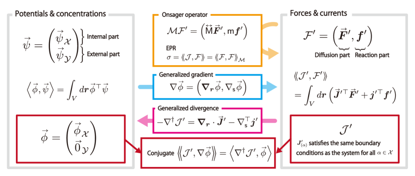
Figure 3: Summary of the vector fields and operators introduced in Sec. III.4. We introduce the generalized gradient operator $\nabla$, taking a potential to a force (indicated in blue), and the generalized divergence $-\nabla^{{\dagger}}$, taking a current to the time evolution caused by the current (pink). We also introduce the Onsager operator $\mathcal{M}$ to represent the linear relationship between the current and force (orange). The inner product $\left\llangle\cdot,\cdot\right\rrangle_{\mathcal{M}}$ induced by $\mathcal{M}$ enables us to rewrite the EPR as the squared norm of the force as $\left\llangle\mathcal{F},\mathcal{F}\right\rrangle_{\mathcal{M}}$. $\nabla$ and $\nabla^{{\dagger}}$ are conjugated when we consider a current, whose $\alpha$-th diffusion part satisfies the same boundary condition imposed on the system for all $\alpha\in\mathcal{X}$, and a potential, whose external part is the zero vector (red).

We consider the quantities associated with reaction and diffusion separately in the previous sections. However, treating these quantities together will be useful for further discussion. Here, we introduce two inner products and some operators to handle reactions and diffusion together. We also show the quantities introduced in this section in Fig. 3.

Forces and currents— Firstly, we introduce the force $\mathcal{F}$ and the current $\mathcal{J}$ by unifying the diffusion force (current) and the reaction force (current) as

$$\mathcal{J}\coloneqq\left(\mathchoice{\kern-0.15pt\overset{\kern 0.7pt\smash{\lower 1.07639pt\hbox{\scalebox{0.45}{$\bm{\rightarrow}$}}}\kern-0.3pt}{\bm{J}}}{\kern-0.15pt\overset{\kern 0.7pt\smash{\lower 1.07639pt\hbox{\scalebox{0.45}{$\bm{\rightarrow}$}}}\kern-0.3pt}{\bm{J}}}{\overset{\smash{\lower 0.6458pt\hbox{\kern 0.2pt\scalebox{0.3}{$\bm{\rightarrow}$}\kern-0.8pt}}}{\bm{J}}}{\overset{\smash{\lower 0.6458pt\hbox{\kern 0.2pt\scalebox{0.3}{$\bm{\rightarrow}$}\kern-0.8pt}}}{\bm{J}}},\bm{j}\right),\quad\mathcal{F}\coloneqq\left(\mathchoice{\kern-0.15pt\overset{\kern 0.7pt\smash{\lower 1.07639pt\hbox{\scalebox{0.45}{$\bm{\rightarrow}$}}}\kern-0.3pt}{\bm{F}}}{\kern-0.15pt\overset{\kern 0.7pt\smash{\lower 1.07639pt\hbox{\scalebox{0.45}{$\bm{\rightarrow}$}}}\kern-0.3pt}{\bm{F}}}{\overset{\smash{\lower 0.6458pt\hbox{\kern 0.2pt\scalebox{0.3}{$\bm{\rightarrow}$}\kern-0.8pt}}}{\bm{F}}}{\overset{\smash{\lower 0.6458pt\hbox{\kern 0.2pt\scalebox{0.3}{$\bm{\rightarrow}$}\kern-0.8pt}}}{\bm{F}}},\bm{f}\right).$$ (74)

We refer to $\mathchoice{\kern-0.15pt\overset{\kern 0.7pt\smash{\lower 1.07639pt\hbox{\scalebox{0.45}{$\bm{\rightarrow}$}}}\kern-0.3pt}{\bm{F}}}{\kern-0.15pt\overset{\kern 0.7pt\smash{\lower 1.07639pt\hbox{\scalebox{0.45}{$\bm{\rightarrow}$}}}\kern-0.3pt}{\bm{F}}}{\overset{\smash{\lower 0.6458pt\hbox{\kern 0.2pt\scalebox{0.3}{$\bm{\rightarrow}$}\kern-0.8pt}}}{\bm{F}}}{\overset{\smash{\lower 0.6458pt\hbox{\kern 0.2pt\scalebox{0.3}{$\bm{\rightarrow}$}\kern-0.8pt}}}{\bm{F}}}{}^{\prime}$ and $\bm{f}^{\prime}$ as the diffusion part and the reaction part of $\mathcal{F}^{\prime}=(\mathchoice{\kern-0.15pt\overset{\kern 0.7pt\smash{\lower 1.07639pt\hbox{\scalebox{0.45}{$\bm{\rightarrow}$}}}\kern-0.3pt}{\bm{F}}}{\kern-0.15pt\overset{\kern 0.7pt\smash{\lower 1.07639pt\hbox{\scalebox{0.45}{$\bm{\rightarrow}$}}}\kern-0.3pt}{\bm{F}}}{\overset{\smash{\lower 0.6458pt\hbox{\kern 0.2pt\scalebox{0.3}{$\bm{\rightarrow}$}\kern-0.8pt}}}{\bm{F}}}{\overset{\smash{\lower 0.6458pt\hbox{\kern 0.2pt\scalebox{0.3}{$\bm{\rightarrow}$}\kern-0.8pt}}}{\bm{F}}}{}^{\prime},\bm{f}^{\prime})$ respectively. Then, the diffusion force $\mathchoice{\kern-0.15pt\overset{\kern 0.7pt\smash{\lower 1.07639pt\hbox{\scalebox{0.45}{$\bm{\rightarrow}$}}}\kern-0.3pt}{\bm{F}}}{\kern-0.15pt\overset{\kern 0.7pt\smash{\lower 1.07639pt\hbox{\scalebox{0.45}{$\bm{\rightarrow}$}}}\kern-0.3pt}{\bm{F}}}{\overset{\smash{\lower 0.6458pt\hbox{\kern 0.2pt\scalebox{0.3}{$\bm{\rightarrow}$}\kern-0.8pt}}}{\bm{F}}}{\overset{\smash{\lower 0.6458pt\hbox{\kern 0.2pt\scalebox{0.3}{$\bm{\rightarrow}$}\kern-0.8pt}}}{\bm{F}}}$ is the diffusion part of the force $\mathcal{F}$, the reaction force $\bm{f}$ is the reaction part of the force $\mathcal{F}$, and the same is true for the current. We also define the inner product of two vector fields $\mathcal{J}^{\prime}=(\mathchoice{\kern-0.15pt\overset{\kern 0.7pt\smash{\lower 1.07639pt\hbox{\scalebox{0.45}{$\bm{\rightarrow}$}}}\kern-0.3pt}{\bm{J}^{\prime}}}{\kern-0.15pt\overset{\kern 0.7pt\smash{\lower 1.07639pt\hbox{\scalebox{0.45}{$\bm{\rightarrow}$}}}\kern-0.3pt}{\bm{J}^{\prime}}}{\overset{\smash{\lower 0.6458pt\hbox{\kern 0.2pt\scalebox{0.3}{$\bm{\rightarrow}$}\kern-0.8pt}}}{\bm{J}^{\prime}}}{\overset{\smash{\lower 0.6458pt\hbox{\kern 0.2pt\scalebox{0.3}{$\bm{\rightarrow}$}\kern-0.8pt}}}{\bm{J}^{\prime}}},\bm{j}^{\prime})$ and $\mathcal{F}^{\prime}=(\mathchoice{\kern-0.15pt\overset{\kern 0.7pt\smash{\lower 1.07639pt\hbox{\scalebox{0.45}{$\bm{\rightarrow}$}}}\kern-0.3pt}{\bm{F}^{\prime}}}{\kern-0.15pt\overset{\kern 0.7pt\smash{\lower 1.07639pt\hbox{\scalebox{0.45}{$\bm{\rightarrow}$}}}\kern-0.3pt}{\bm{F}^{\prime}}}{\overset{\smash{\lower 0.6458pt\hbox{\kern 0.2pt\scalebox{0.3}{$\bm{\rightarrow}$}\kern-0.8pt}}}{\bm{F}^{\prime}}}{\overset{\smash{\lower 0.6458pt\hbox{\kern 0.2pt\scalebox{0.3}{$\bm{\rightarrow}$}\kern-0.8pt}}}{\bm{F}^{\prime}}},\bm{f}^{\prime})$ as

$$\left\llangle\mathcal{J}^{\prime},\mathcal{F}^{\prime}\right\rrangle \coloneqq\int_{V}d\bm{r}\quantity(\sum_{\alpha\in\mathcal{S}}\bm{J}_{\alpha}^{\prime}\cdot\bm{F}_{\alpha}^{\prime}+\sum_{\rho\in\mathcal{R}}j_{\rho}^{\prime}f_{\rho}^{\prime})$$

$$=\int_{V}d\bm{r}\quantity(\mathchoice{\kern-0.15pt\overset{\kern 0.7pt\smash{\lower 1.07639pt\hbox{\scalebox{0.45}{$\bm{\rightarrow}$}}}\kern-0.3pt}{\bm{J}^{\prime}}}{\kern-0.15pt\overset{\kern 0.7pt\smash{\lower 1.07639pt\hbox{\scalebox{0.45}{$\bm{\rightarrow}$}}}\kern-0.3pt}{\bm{J}^{\prime}}}{\overset{\smash{\lower 0.6458pt\hbox{\kern 0.2pt\scalebox{0.3}{$\bm{\rightarrow}$}\kern-0.8pt}}}{\bm{J}^{\prime}}}{\overset{\smash{\lower 0.6458pt\hbox{\kern 0.2pt\scalebox{0.3}{$\bm{\rightarrow}$}\kern-0.8pt}}}{\bm{J}^{\prime}}}{}^{\top}\mathchoice{\kern-0.15pt\overset{\kern 0.7pt\smash{\lower 1.07639pt\hbox{\scalebox{0.45}{$\bm{\rightarrow}$}}}\kern-0.3pt}{\bm{F}^{\prime}}}{\kern-0.15pt\overset{\kern 0.7pt\smash{\lower 1.07639pt\hbox{\scalebox{0.45}{$\bm{\rightarrow}$}}}\kern-0.3pt}{\bm{F}^{\prime}}}{\overset{\smash{\lower 0.6458pt\hbox{\kern 0.2pt\scalebox{0.3}{$\bm{\rightarrow}$}\kern-0.8pt}}}{\bm{F}^{\prime}}}{\overset{\smash{\lower 0.6458pt\hbox{\kern 0.2pt\scalebox{0.3}{$\bm{\rightarrow}$}\kern-0.8pt}}}{\bm{F}^{\prime}}}+\bm{j}^{\prime}{}^{\top}\bm{f}^{\prime}),$$ (75)

which immediately leads to a new expression of the EPR as

$$\sigma=\left\llangle\mathcal{J},\mathcal{F}\right\rrangle.$$ (76)

Potentials and concentrations— We introduce the inner product of two vector fields with $N$ elements, e.g., the chemical potential $\mathchoice{\kern-0.15pt\overset{\kern 0.7pt\smash{\lower 1.07639pt\hbox{\scalebox{0.45}{$\bm{\rightarrow}$}}}\kern-0.3pt}{\mu}}{\kern-0.15pt\overset{\kern 0.7pt\smash{\lower 1.07639pt\hbox{\scalebox{0.45}{$\bm{\rightarrow}$}}}\kern-0.3pt}{\mu}}{\overset{\smash{\lower 0.6458pt\hbox{\kern 0.2pt\scalebox{0.3}{$\bm{\rightarrow}$}\kern-0.8pt}}}{\mu}}{\overset{\smash{\lower 0.6458pt\hbox{\kern 0.2pt\scalebox{0.3}{$\bm{\rightarrow}$}\kern-0.8pt}}}{\mu}}$, the concentration distribution $\mathchoice{\kern-0.15pt\overset{\kern 0.7pt\smash{\lower 1.07639pt\hbox{\scalebox{0.45}{$\bm{\rightarrow}$}}}\kern-0.3pt}{c}}{\kern-0.15pt\overset{\kern 0.7pt\smash{\lower 1.07639pt\hbox{\scalebox{0.45}{$\bm{\rightarrow}$}}}\kern-0.3pt}{c}}{\overset{\smash{\lower 0.6458pt\hbox{\kern 0.2pt\scalebox{0.3}{$\bm{\rightarrow}$}\kern-0.8pt}}}{c}}{\overset{\smash{\lower 0.6458pt\hbox{\kern 0.2pt\scalebox{0.3}{$\bm{\rightarrow}$}\kern-0.8pt}}}{c}}$, and its time derivative $\partial_{t}\mathchoice{\kern-0.15pt\overset{\kern 0.7pt\smash{\lower 1.07639pt\hbox{\scalebox{0.45}{$\bm{\rightarrow}$}}}\kern-0.3pt}{c}}{\kern-0.15pt\overset{\kern 0.7pt\smash{\lower 1.07639pt\hbox{\scalebox{0.45}{$\bm{\rightarrow}$}}}\kern-0.3pt}{c}}{\overset{\smash{\lower 0.6458pt\hbox{\kern 0.2pt\scalebox{0.3}{$\bm{\rightarrow}$}\kern-0.8pt}}}{c}}{\overset{\smash{\lower 0.6458pt\hbox{\kern 0.2pt\scalebox{0.3}{$\bm{\rightarrow}$}\kern-0.8pt}}}{c}}$, as

$$\left\langle\mathchoice{\kern-0.15pt\overset{\kern 0.7pt\smash{\lower 1.07639pt\hbox{\scalebox{0.45}{$\bm{\rightarrow}$}}}\kern-0.3pt}{\phi}}{\kern-0.15pt\overset{\kern 0.7pt\smash{\lower 1.07639pt\hbox{\scalebox{0.45}{$\bm{\rightarrow}$}}}\kern-0.3pt}{\phi}}{\overset{\smash{\lower 0.6458pt\hbox{\kern 0.2pt\scalebox{0.3}{$\bm{\rightarrow}$}\kern-0.8pt}}}{\phi}}{\overset{\smash{\lower 0.6458pt\hbox{\kern 0.2pt\scalebox{0.3}{$\bm{\rightarrow}$}\kern-0.8pt}}}{\phi}},\mathchoice{\kern-0.15pt\overset{\kern 0.7pt\smash{\lower 1.07639pt\hbox{\scalebox{0.45}{$\bm{\rightarrow}$}}}\kern-0.3pt}{\psi}}{\kern-0.15pt\overset{\kern 0.7pt\smash{\lower 1.07639pt\hbox{\scalebox{0.45}{$\bm{\rightarrow}$}}}\kern-0.3pt}{\psi}}{\overset{\smash{\lower 0.6458pt\hbox{\kern 0.2pt\scalebox{0.3}{$\bm{\rightarrow}$}\kern-0.8pt}}}{\psi}}{\overset{\smash{\lower 0.6458pt\hbox{\kern 0.2pt\scalebox{0.3}{$\bm{\rightarrow}$}\kern-0.8pt}}}{\psi}}\right\rangle\coloneqq\int_{V}d\bm{r}\sum_{\alpha\in\mathcal{S}}\phi_{\alpha}\psi_{\alpha}=\int_{V}d\bm{r}\mathchoice{\kern-0.15pt\overset{\kern 0.7pt\smash{\lower 1.07639pt\hbox{\scalebox{0.45}{$\bm{\rightarrow}$}}}\kern-0.3pt}{\phi}}{\kern-0.15pt\overset{\kern 0.7pt\smash{\lower 1.07639pt\hbox{\scalebox{0.45}{$\bm{\rightarrow}$}}}\kern-0.3pt}{\phi}}{\overset{\smash{\lower 0.6458pt\hbox{\kern 0.2pt\scalebox{0.3}{$\bm{\rightarrow}$}\kern-0.8pt}}}{\phi}}{\overset{\smash{\lower 0.6458pt\hbox{\kern 0.2pt\scalebox{0.3}{$\bm{\rightarrow}$}\kern-0.8pt}}}{\phi}}\>{}^{\top}\mathchoice{\kern-0.15pt\overset{\kern 0.7pt\smash{\lower 1.07639pt\hbox{\scalebox{0.45}{$\bm{\rightarrow}$}}}\kern-0.3pt}{\psi}}{\kern-0.15pt\overset{\kern 0.7pt\smash{\lower 1.07639pt\hbox{\scalebox{0.45}{$\bm{\rightarrow}$}}}\kern-0.3pt}{\psi}}{\overset{\smash{\lower 0.6458pt\hbox{\kern 0.2pt\scalebox{0.3}{$\bm{\rightarrow}$}\kern-0.8pt}}}{\psi}}{\overset{\smash{\lower 0.6458pt\hbox{\kern 0.2pt\scalebox{0.3}{$\bm{\rightarrow}$}\kern-0.8pt}}}{\psi}},$$ (77)

with $\mathchoice{\kern-0.15pt\overset{\kern 0.7pt\smash{\lower 1.07639pt\hbox{\scalebox{0.45}{$\bm{\rightarrow}$}}}\kern-0.3pt}{\phi}}{\kern-0.15pt\overset{\kern 0.7pt\smash{\lower 1.07639pt\hbox{\scalebox{0.45}{$\bm{\rightarrow}$}}}\kern-0.3pt}{\phi}}{\overset{\smash{\lower 0.6458pt\hbox{\kern 0.2pt\scalebox{0.3}{$\bm{\rightarrow}$}\kern-0.8pt}}}{\phi}}{\overset{\smash{\lower 0.6458pt\hbox{\kern 0.2pt\scalebox{0.3}{$\bm{\rightarrow}$}\kern-0.8pt}}}{\phi}}=(\phi_{1},\dots,\phi_{N})^{\top}$ and $\mathchoice{\kern-0.15pt\overset{\kern 0.7pt\smash{\lower 1.07639pt\hbox{\scalebox{0.45}{$\bm{\rightarrow}$}}}\kern-0.3pt}{\psi}}{\kern-0.15pt\overset{\kern 0.7pt\smash{\lower 1.07639pt\hbox{\scalebox{0.45}{$\bm{\rightarrow}$}}}\kern-0.3pt}{\psi}}{\overset{\smash{\lower 0.6458pt\hbox{\kern 0.2pt\scalebox{0.3}{$\bm{\rightarrow}$}\kern-0.8pt}}}{\psi}}{\overset{\smash{\lower 0.6458pt\hbox{\kern 0.2pt\scalebox{0.3}{$\bm{\rightarrow}$}\kern-0.8pt}}}{\psi}}=(\psi_{1},\dots,\psi_{N})^{\top}$. We refer to $\mathchoice{\kern-0.15pt\overset{\kern 0.7pt\smash{\lower 1.07639pt\hbox{\scalebox{0.45}{$\bm{\rightarrow}$}}}\kern-0.3pt}{\psi}}{\kern-0.15pt\overset{\kern 0.7pt\smash{\lower 1.07639pt\hbox{\scalebox{0.45}{$\bm{\rightarrow}$}}}\kern-0.3pt}{\psi}}{\overset{\smash{\lower 0.6458pt\hbox{\kern 0.2pt\scalebox{0.3}{$\bm{\rightarrow}$}\kern-0.8pt}}}{\psi}}{\overset{\smash{\lower 0.6458pt\hbox{\kern 0.2pt\scalebox{0.3}{$\bm{\rightarrow}$}\kern-0.8pt}}}{\psi}}_{\mathcal{X}}=(\psi_{1},\dots,\psi_{N_{\mathcal{X}}})^{\top}$ and $\mathchoice{\kern-0.15pt\overset{\kern 0.7pt\smash{\lower 1.07639pt\hbox{\scalebox{0.45}{$\bm{\rightarrow}$}}}\kern-0.3pt}{\psi}}{\kern-0.15pt\overset{\kern 0.7pt\smash{\lower 1.07639pt\hbox{\scalebox{0.45}{$\bm{\rightarrow}$}}}\kern-0.3pt}{\psi}}{\overset{\smash{\lower 0.6458pt\hbox{\kern 0.2pt\scalebox{0.3}{$\bm{\rightarrow}$}\kern-0.8pt}}}{\psi}}{\overset{\smash{\lower 0.6458pt\hbox{\kern 0.2pt\scalebox{0.3}{$\bm{\rightarrow}$}\kern-0.8pt}}}{\psi}}_{\mathcal{Y}}=(\psi_{N_{\mathcal{X}}+1},\dots,\psi_{N})^{\top}$ as the internal part and the external part of $\mathchoice{\kern-0.15pt\overset{\kern 0.7pt\smash{\lower 1.07639pt\hbox{\scalebox{0.45}{$\bm{\rightarrow}$}}}\kern-0.3pt}{\psi}}{\kern-0.15pt\overset{\kern 0.7pt\smash{\lower 1.07639pt\hbox{\scalebox{0.45}{$\bm{\rightarrow}$}}}\kern-0.3pt}{\psi}}{\overset{\smash{\lower 0.6458pt\hbox{\kern 0.2pt\scalebox{0.3}{$\bm{\rightarrow}$}\kern-0.8pt}}}{\psi}}{\overset{\smash{\lower 0.6458pt\hbox{\kern 0.2pt\scalebox{0.3}{$\bm{\rightarrow}$}\kern-0.8pt}}}{\psi}}=(\psi_{1},\dots,\psi_{N})^{\top}$, a vector field with $N$ elements, e.g., $\partial_{t}\mathchoice{\kern-0.15pt\overset{\kern 0.7pt\smash{\lower 1.07639pt\hbox{\scalebox{0.45}{$\bm{\rightarrow}$}}}\kern-0.3pt}{c}}{\kern-0.15pt\overset{\kern 0.7pt\smash{\lower 1.07639pt\hbox{\scalebox{0.45}{$\bm{\rightarrow}$}}}\kern-0.3pt}{c}}{\overset{\smash{\lower 0.6458pt\hbox{\kern 0.2pt\scalebox{0.3}{$\bm{\rightarrow}$}\kern-0.8pt}}}{c}}{\overset{\smash{\lower 0.6458pt\hbox{\kern 0.2pt\scalebox{0.3}{$\bm{\rightarrow}$}\kern-0.8pt}}}{c}}_{\mathcal{X}}=(\partial_{t}c_{1},\dots,\partial_{t}c_{N_{\mathcal{X}}})^{\top}$ is the internal part of $\partial_{t}\mathchoice{\kern-0.15pt\overset{\kern 0.7pt\smash{\lower 1.07639pt\hbox{\scalebox{0.45}{$\bm{\rightarrow}$}}}\kern-0.3pt}{c}}{\kern-0.15pt\overset{\kern 0.7pt\smash{\lower 1.07639pt\hbox{\scalebox{0.45}{$\bm{\rightarrow}$}}}\kern-0.3pt}{c}}{\overset{\smash{\lower 0.6458pt\hbox{\kern 0.2pt\scalebox{0.3}{$\bm{\rightarrow}$}\kern-0.8pt}}}{c}}{\overset{\smash{\lower 0.6458pt\hbox{\kern 0.2pt\scalebox{0.3}{$\bm{\rightarrow}$}\kern-0.8pt}}}{c}}=(\partial_{t}c_{1},\dots,\partial_{t}c_{N})^{\top}$.

Generalized gradient and divergence operators— We define the generalized gradient operator $\nabla$, taking a potential $\mathchoice{\kern-0.15pt\overset{\kern 0.7pt\smash{\lower 1.07639pt\hbox{\scalebox{0.45}{$\bm{\rightarrow}$}}}\kern-0.3pt}{\phi}}{\kern-0.15pt\overset{\kern 0.7pt\smash{\lower 1.07639pt\hbox{\scalebox{0.45}{$\bm{\rightarrow}$}}}\kern-0.3pt}{\phi}}{\overset{\smash{\lower 0.6458pt\hbox{\kern 0.2pt\scalebox{0.3}{$\bm{\rightarrow}$}\kern-0.8pt}}}{\phi}}{\overset{\smash{\lower 0.6458pt\hbox{\kern 0.2pt\scalebox{0.3}{$\bm{\rightarrow}$}\kern-0.8pt}}}{\phi}}=(\phi_{1},\dots,\phi_{N}){}^{\top}$ to a force, as

$$\nabla\mathchoice{\kern-0.15pt\overset{\kern 0.7pt\smash{\lower 1.07639pt\hbox{\scalebox{0.45}{$\bm{\rightarrow}$}}}\kern-0.3pt}{\phi}}{\kern-0.15pt\overset{\kern 0.7pt\smash{\lower 1.07639pt\hbox{\scalebox{0.45}{$\bm{\rightarrow}$}}}\kern-0.3pt}{\phi}}{\overset{\smash{\lower 0.6458pt\hbox{\kern 0.2pt\scalebox{0.3}{$\bm{\rightarrow}$}\kern-0.8pt}}}{\phi}}{\overset{\smash{\lower 0.6458pt\hbox{\kern 0.2pt\scalebox{0.3}{$\bm{\rightarrow}$}\kern-0.8pt}}}{\phi}}\coloneqq(\bm{\nabla}_{\bm{r}}\mathchoice{\kern-0.15pt\overset{\kern 0.7pt\smash{\lower 1.07639pt\hbox{\scalebox{0.45}{$\bm{\rightarrow}$}}}\kern-0.3pt}{\phi}}{\kern-0.15pt\overset{\kern 0.7pt\smash{\lower 1.07639pt\hbox{\scalebox{0.45}{$\bm{\rightarrow}$}}}\kern-0.3pt}{\phi}}{\overset{\smash{\lower 0.6458pt\hbox{\kern 0.2pt\scalebox{0.3}{$\bm{\rightarrow}$}\kern-0.8pt}}}{\phi}}{\overset{\smash{\lower 0.6458pt\hbox{\kern 0.2pt\scalebox{0.3}{$\bm{\rightarrow}$}\kern-0.8pt}}}{\phi}},\nabla_{\mathsf{s}}\mathchoice{\kern-0.15pt\overset{\kern 0.7pt\smash{\lower 1.07639pt\hbox{\scalebox{0.45}{$\bm{\rightarrow}$}}}\kern-0.3pt}{\phi}}{\kern-0.15pt\overset{\kern 0.7pt\smash{\lower 1.07639pt\hbox{\scalebox{0.45}{$\bm{\rightarrow}$}}}\kern-0.3pt}{\phi}}{\overset{\smash{\lower 0.6458pt\hbox{\kern 0.2pt\scalebox{0.3}{$\bm{\rightarrow}$}\kern-0.8pt}}}{\phi}}{\overset{\smash{\lower 0.6458pt\hbox{\kern 0.2pt\scalebox{0.3}{$\bm{\rightarrow}$}\kern-0.8pt}}}{\phi}}),$$ (78)

where $\bm{\nabla}_{\bm{r}}\mathchoice{\kern-0.15pt\overset{\kern 0.7pt\smash{\lower 1.07639pt\hbox{\scalebox{0.45}{$\bm{\rightarrow}$}}}\kern-0.3pt}{\phi}}{\kern-0.15pt\overset{\kern 0.7pt\smash{\lower 1.07639pt\hbox{\scalebox{0.45}{$\bm{\rightarrow}$}}}\kern-0.3pt}{\phi}}{\overset{\smash{\lower 0.6458pt\hbox{\kern 0.2pt\scalebox{0.3}{$\bm{\rightarrow}$}\kern-0.8pt}}}{\phi}}{\overset{\smash{\lower 0.6458pt\hbox{\kern 0.2pt\scalebox{0.3}{$\bm{\rightarrow}$}\kern-0.8pt}}}{\phi}}$ is defined as $\bm{\nabla}_{\bm{r}}\mathchoice{\kern-0.15pt\overset{\kern 0.7pt\smash{\lower 1.07639pt\hbox{\scalebox{0.45}{$\bm{\rightarrow}$}}}\kern-0.3pt}{\phi}}{\kern-0.15pt\overset{\kern 0.7pt\smash{\lower 1.07639pt\hbox{\scalebox{0.45}{$\bm{\rightarrow}$}}}\kern-0.3pt}{\phi}}{\overset{\smash{\lower 0.6458pt\hbox{\kern 0.2pt\scalebox{0.3}{$\bm{\rightarrow}$}\kern-0.8pt}}}{\phi}}{\overset{\smash{\lower 0.6458pt\hbox{\kern 0.2pt\scalebox{0.3}{$\bm{\rightarrow}$}\kern-0.8pt}}}{\phi}}\coloneqq(\bm{\nabla}_{\bm{r}}\phi_{1},\dots,\bm{\nabla}_{\bm{r}}\phi_{N}){}^{\top}$. We remark that $\nabla_{\mathsf{s}}\mathchoice{\kern-0.15pt\overset{\kern 0.7pt\smash{\lower 1.07639pt\hbox{\scalebox{0.45}{$\bm{\rightarrow}$}}}\kern-0.3pt}{\phi}}{\kern-0.15pt\overset{\kern 0.7pt\smash{\lower 1.07639pt\hbox{\scalebox{0.45}{$\bm{\rightarrow}$}}}\kern-0.3pt}{\phi}}{\overset{\smash{\lower 0.6458pt\hbox{\kern 0.2pt\scalebox{0.3}{$\bm{\rightarrow}$}\kern-0.8pt}}}{\phi}}{\overset{\smash{\lower 0.6458pt\hbox{\kern 0.2pt\scalebox{0.3}{$\bm{\rightarrow}$}\kern-0.8pt}}}{\phi}}(\bm{r})$ is an $M$-dimensional vector because $\nabla_{\mathsf{s}}$ is an $M\times N$ matrix and $\mathchoice{\kern-0.15pt\overset{\kern 0.7pt\smash{\lower 1.07639pt\hbox{\scalebox{0.45}{$\bm{\rightarrow}$}}}\kern-0.3pt}{\phi}}{\kern-0.15pt\overset{\kern 0.7pt\smash{\lower 1.07639pt\hbox{\scalebox{0.45}{$\bm{\rightarrow}$}}}\kern-0.3pt}{\phi}}{\overset{\smash{\lower 0.6458pt\hbox{\kern 0.2pt\scalebox{0.3}{$\bm{\rightarrow}$}\kern-0.8pt}}}{\phi}}{\overset{\smash{\lower 0.6458pt\hbox{\kern 0.2pt\scalebox{0.3}{$\bm{\rightarrow}$}\kern-0.8pt}}}{\phi}}(\bm{r})$ is an $N$-dimensional vector. The generalized gradient operator $\nabla=\bm{\nabla}_{\bm{r}}\oplus\nabla_{\mathsf{s}}$ is regarded as the direct sum between $\bm{\nabla}_{\bm{r}}$ and $\nabla_{\mathsf{s}}$, where $\oplus$ stands for the direct sum.

The generalized gradient $\nabla$ enables us to unify the relations between the diffusion and reaction forces and the chemical potential in Eq. (57) and Eq. (62) as

$$\mathcal{F}=-\nabla\mathchoice{\kern-0.15pt\overset{\kern 0.7pt\smash{\lower 1.07639pt\hbox{\scalebox{0.45}{$\bm{\rightarrow}$}}}\kern-0.3pt}{\mu}}{\kern-0.15pt\overset{\kern 0.7pt\smash{\lower 1.07639pt\hbox{\scalebox{0.45}{$\bm{\rightarrow}$}}}\kern-0.3pt}{\mu}}{\overset{\smash{\lower 0.6458pt\hbox{\kern 0.2pt\scalebox{0.3}{$\bm{\rightarrow}$}\kern-0.8pt}}}{\mu}}{\overset{\smash{\lower 0.6458pt\hbox{\kern 0.2pt\scalebox{0.3}{$\bm{\rightarrow}$}\kern-0.8pt}}}{\mu}}+\mathcal{K}^{\mathrm{nc}},$$ (79)

where we define the nonconservative mechanical force vector $\mathcal{K}^{\mathrm{nc}}$ as $\mathcal{K}^{\mathrm{nc}}\coloneqq(\mathchoice{\kern-0.15pt\overset{\kern 0.7pt\smash{\lower 1.07639pt\hbox{\scalebox{0.45}{$\bm{\rightarrow}$}}}\kern-0.3pt}{\bm{K}}}{\kern-0.15pt\overset{\kern 0.7pt\smash{\lower 1.07639pt\hbox{\scalebox{0.45}{$\bm{\rightarrow}$}}}\kern-0.3pt}{\bm{K}}}{\overset{\smash{\lower 0.6458pt\hbox{\kern 0.2pt\scalebox{0.3}{$\bm{\rightarrow}$}\kern-0.8pt}}}{\bm{K}}}{\overset{\smash{\lower 0.6458pt\hbox{\kern 0.2pt\scalebox{0.3}{$\bm{\rightarrow}$}\kern-0.8pt}}}{\bm{K}}}{}^{\mathrm{nc}},\bm{0})$.

We also define an operator $\nabla^{{\dagger}}$ that maps a current to the time evolution caused by the current as

$$\nabla^{{\dagger}}\mathcal{J}^{\prime}\coloneqq-\bm{\nabla}_{\bm{r}}\cdot\mathchoice{\kern-0.15pt\overset{\kern 0.7pt\smash{\lower 1.07639pt\hbox{\scalebox{0.45}{$\bm{\rightarrow}$}}}\kern-0.3pt}{\bm{J}}}{\kern-0.15pt\overset{\kern 0.7pt\smash{\lower 1.07639pt\hbox{\scalebox{0.45}{$\bm{\rightarrow}$}}}\kern-0.3pt}{\bm{J}}}{\overset{\smash{\lower 0.6458pt\hbox{\kern 0.2pt\scalebox{0.3}{$\bm{\rightarrow}$}\kern-0.8pt}}}{\bm{J}}}{\overset{\smash{\lower 0.6458pt\hbox{\kern 0.2pt\scalebox{0.3}{$\bm{\rightarrow}$}\kern-0.8pt}}}{\bm{J}}}{}^{\prime}+\nabla_{\mathsf{s}}^{\top}\bm{j}^{\prime},$$ (80)

where $\mathcal{J}^{\prime}=(\mathchoice{\kern-0.15pt\overset{\kern 0.7pt\smash{\lower 1.07639pt\hbox{\scalebox{0.45}{$\bm{\rightarrow}$}}}\kern-0.3pt}{\bm{J}^{\prime}}}{\kern-0.15pt\overset{\kern 0.7pt\smash{\lower 1.07639pt\hbox{\scalebox{0.45}{$\bm{\rightarrow}$}}}\kern-0.3pt}{\bm{J}^{\prime}}}{\overset{\smash{\lower 0.6458pt\hbox{\kern 0.2pt\scalebox{0.3}{$\bm{\rightarrow}$}\kern-0.8pt}}}{\bm{J}^{\prime}}}{\overset{\smash{\lower 0.6458pt\hbox{\kern 0.2pt\scalebox{0.3}{$\bm{\rightarrow}$}\kern-0.8pt}}}{\bm{J}^{\prime}}},\bm{j}^{\prime})$ is a vector field with the reaction and diffusion parts, and $\nabla^{{\dagger}}\mathcal{J}^{\prime}$ is a vector field with $N$ elements. This definition means $-\nabla^{{\dagger}}$ is a generalized divergence operator. Using the operator $\nabla^{{\dagger}}$, the time evolution of the internal species in RDSs in Eq. (55) is written as

$$\partial_{t}\mathchoice{\kern-0.15pt\overset{\kern 0.7pt\smash{\lower 1.07639pt\hbox{\scalebox{0.45}{$\bm{\rightarrow}$}}}\kern-0.3pt}{c}}{\kern-0.15pt\overset{\kern 0.7pt\smash{\lower 1.07639pt\hbox{\scalebox{0.45}{$\bm{\rightarrow}$}}}\kern-0.3pt}{c}}{\overset{\smash{\lower 0.6458pt\hbox{\kern 0.2pt\scalebox{0.3}{$\bm{\rightarrow}$}\kern-0.8pt}}}{c}}{\overset{\smash{\lower 0.6458pt\hbox{\kern 0.2pt\scalebox{0.3}{$\bm{\rightarrow}$}\kern-0.8pt}}}{c}}_{\mathcal{X}}=\quantity(\nabla^{{\dagger}}\mathcal{J})_{\mathcal{X}}.$$ (81)

The operator $\nabla^{{\dagger}}$ is conjugate to the generalized gradient operator $\nabla$ in terms of the two inner products $\left\llangle\cdot,\cdot\right\rrangle$ and $\left\langle\cdot,\cdot\right\rangle$ as

$$\left\llangle\mathcal{J}^{\prime},\nabla\mathchoice{\kern-0.15pt\overset{\kern 0.7pt\smash{\lower 1.07639pt\hbox{\scalebox{0.45}{$\bm{\rightarrow}$}}}\kern-0.3pt}{\phi}}{\kern-0.15pt\overset{\kern 0.7pt\smash{\lower 1.07639pt\hbox{\scalebox{0.45}{$\bm{\rightarrow}$}}}\kern-0.3pt}{\phi}}{\overset{\smash{\lower 0.6458pt\hbox{\kern 0.2pt\scalebox{0.3}{$\bm{\rightarrow}$}\kern-0.8pt}}}{\phi}}{\overset{\smash{\lower 0.6458pt\hbox{\kern 0.2pt\scalebox{0.3}{$\bm{\rightarrow}$}\kern-0.8pt}}}{\phi}}\right\rrangle=\left\langle\nabla^{{\dagger}}\mathcal{J}^{\prime},\mathchoice{\kern-0.15pt\overset{\kern 0.7pt\smash{\lower 1.07639pt\hbox{\scalebox{0.45}{$\bm{\rightarrow}$}}}\kern-0.3pt}{\phi}}{\kern-0.15pt\overset{\kern 0.7pt\smash{\lower 1.07639pt\hbox{\scalebox{0.45}{$\bm{\rightarrow}$}}}\kern-0.3pt}{\phi}}{\overset{\smash{\lower 0.6458pt\hbox{\kern 0.2pt\scalebox{0.3}{$\bm{\rightarrow}$}\kern-0.8pt}}}{\phi}}{\overset{\smash{\lower 0.6458pt\hbox{\kern 0.2pt\scalebox{0.3}{$\bm{\rightarrow}$}\kern-0.8pt}}}{\phi}}\right\rangle,$$ (82)

where $\mathchoice{\kern-0.15pt\overset{\kern 0.7pt\smash{\lower 1.07639pt\hbox{\scalebox{0.45}{$\bm{\rightarrow}$}}}\kern-0.3pt}{\phi}}{\kern-0.15pt\overset{\kern 0.7pt\smash{\lower 1.07639pt\hbox{\scalebox{0.45}{$\bm{\rightarrow}$}}}\kern-0.3pt}{\phi}}{\overset{\smash{\lower 0.6458pt\hbox{\kern 0.2pt\scalebox{0.3}{$\bm{\rightarrow}$}\kern-0.8pt}}}{\phi}}{\overset{\smash{\lower 0.6458pt\hbox{\kern 0.2pt\scalebox{0.3}{$\bm{\rightarrow}$}\kern-0.8pt}}}{\phi}}$ is a potential whose external part is the zero vector, and $\mathcal{J}^{\prime}$ is a current whose diffusion part corresponds to the internal species, $\bm{J}^{\prime}_{(\alpha)}$ for $\alpha\in\mathcal{X}$, satisfies the boundary conditions on the system. To derive the conjugation relations between $\nabla$ and $\nabla^{{\dagger}}$, we do partial integration and use Gauss’s theorem to calculate $\left\langle\nabla^{{\dagger}}\mathcal{J}^{\prime},\mathchoice{\kern-0.15pt\overset{\kern 0.7pt\smash{\lower 1.07639pt\hbox{\scalebox{0.45}{$\bm{\rightarrow}$}}}\kern-0.3pt}{\phi}}{\kern-0.15pt\overset{\kern 0.7pt\smash{\lower 1.07639pt\hbox{\scalebox{0.45}{$\bm{\rightarrow}$}}}\kern-0.3pt}{\phi}}{\overset{\smash{\lower 0.6458pt\hbox{\kern 0.2pt\scalebox{0.3}{$\bm{\rightarrow}$}\kern-0.8pt}}}{\phi}}{\overset{\smash{\lower 0.6458pt\hbox{\kern 0.2pt\scalebox{0.3}{$\bm{\rightarrow}$}\kern-0.8pt}}}{\phi}}\right\rangle$ as follows:

$$\left\langle\nabla^{{\dagger}}\mathcal{J}^{\prime},\mathchoice{\kern-0.15pt\overset{\kern 0.7pt\smash{\lower 1.07639pt\hbox{\scalebox{0.45}{$\bm{\rightarrow}$}}}\kern-0.3pt}{\phi}}{\kern-0.15pt\overset{\kern 0.7pt\smash{\lower 1.07639pt\hbox{\scalebox{0.45}{$\bm{\rightarrow}$}}}\kern-0.3pt}{\phi}}{\overset{\smash{\lower 0.6458pt\hbox{\kern 0.2pt\scalebox{0.3}{$\bm{\rightarrow}$}\kern-0.8pt}}}{\phi}}{\overset{\smash{\lower 0.6458pt\hbox{\kern 0.2pt\scalebox{0.3}{$\bm{\rightarrow}$}\kern-0.8pt}}}{\phi}}\right\rangle=\int_{V}d\bm{r}\sum_{\alpha\in\mathcal{S}}\quantity{-\bm{\nabla}_{\bm{r}}\cdot\bm{J}^{\prime}_{(\alpha)}+\quantity(\nabla_{\mathsf{s}}^{\top}\bm{j}^{\prime})_{\alpha}}\phi_{\alpha}$$

$$=\int_{V}d\bm{r}\left\{\sum_{\alpha\in\mathcal{S}}\quantity(\bm{J}^{\prime}_{(\alpha)}\cdot\bm{\nabla}_{\bm{r}}\phi_{\alpha})+\bm{j}^{\prime\top}\nabla_{\mathsf{s}}\mathchoice{\kern-0.15pt\overset{\kern 0.7pt\smash{\lower 1.07639pt\hbox{\scalebox{0.45}{$\bm{\rightarrow}$}}}\kern-0.3pt}{\phi}}{\kern-0.15pt\overset{\kern 0.7pt\smash{\lower 1.07639pt\hbox{\scalebox{0.45}{$\bm{\rightarrow}$}}}\kern-0.3pt}{\phi}}{\overset{\smash{\lower 0.6458pt\hbox{\kern 0.2pt\scalebox{0.3}{$\bm{\rightarrow}$}\kern-0.8pt}}}{\phi}}{\overset{\smash{\lower 0.6458pt\hbox{\kern 0.2pt\scalebox{0.3}{$\bm{\rightarrow}$}\kern-0.8pt}}}{\phi}}\right.$$

$$\hskip 125.0pt\left.-\sum_{\alpha\in\mathcal{S}}\bm{\nabla}_{\bm{r}}\cdot\quantity(\phi_{\alpha}\bm{J}^{\prime}_{(\alpha)})\right\}$$

$$=\left\llangle\mathcal{J}^{\prime},\nabla\mathchoice{\kern-0.15pt\overset{\kern 0.7pt\smash{\lower 1.07639pt\hbox{\scalebox{0.45}{$\bm{\rightarrow}$}}}\kern-0.3pt}{\phi}}{\kern-0.15pt\overset{\kern 0.7pt\smash{\lower 1.07639pt\hbox{\scalebox{0.45}{$\bm{\rightarrow}$}}}\kern-0.3pt}{\phi}}{\overset{\smash{\lower 0.6458pt\hbox{\kern 0.2pt\scalebox{0.3}{$\bm{\rightarrow}$}\kern-0.8pt}}}{\phi}}{\overset{\smash{\lower 0.6458pt\hbox{\kern 0.2pt\scalebox{0.3}{$\bm{\rightarrow}$}\kern-0.8pt}}}{\phi}}\right\rrangle-\sum_{\alpha\in\mathcal{S}}\int_{\partial V}d\bm{n}\cdot\quantity(\phi_{\alpha}\bm{J}^{\prime}_{(\alpha)}).$$ (83)

The summands in the second term of the last line, $\int_{\partial V}d\bm{n}\cdot(\phi_{\alpha}\bm{J}^{\prime}_{(\alpha)})$, vanishes because $\phi_{\alpha}=0$ holds for all $\alpha\in\mathcal{Y}$, and $\bm{J}^{\prime}_{(\alpha)}$ satisfies the boundary conditions for all $\alpha\in\mathcal{X}$. Thus, we obtain Eq. (82). We remind the reader that we also impose the periodic boundary condition on every field containing $\mathchoice{\kern-0.15pt\overset{\kern 0.7pt\smash{\lower 1.07639pt\hbox{\scalebox{0.45}{$\bm{\rightarrow}$}}}\kern-0.3pt}{\phi}}{\kern-0.15pt\overset{\kern 0.7pt\smash{\lower 1.07639pt\hbox{\scalebox{0.45}{$\bm{\rightarrow}$}}}\kern-0.3pt}{\phi}}{\overset{\smash{\lower 0.6458pt\hbox{\kern 0.2pt\scalebox{0.3}{$\bm{\rightarrow}$}\kern-0.8pt}}}{\phi}}{\overset{\smash{\lower 0.6458pt\hbox{\kern 0.2pt\scalebox{0.3}{$\bm{\rightarrow}$}\kern-0.8pt}}}{\phi}}$ if we impose it on the system.

The expression in Eq. (82) gives another expression of the EPR in terms of the inner product $\left\langle\cdot,\cdot\right\rangle$ in closed systems without the nonconservative mechanical force, $\mathchoice{\kern-0.15pt\overset{\kern 0.7pt\smash{\lower 1.07639pt\hbox{\scalebox{0.45}{$\bm{\rightarrow}$}}}\kern-0.3pt}{\bm{K}}}{\kern-0.15pt\overset{\kern 0.7pt\smash{\lower 1.07639pt\hbox{\scalebox{0.45}{$\bm{\rightarrow}$}}}\kern-0.3pt}{\bm{K}}}{\overset{\smash{\lower 0.6458pt\hbox{\kern 0.2pt\scalebox{0.3}{$\bm{\rightarrow}$}\kern-0.8pt}}}{\bm{K}}}{\overset{\smash{\lower 0.6458pt\hbox{\kern 0.2pt\scalebox{0.3}{$\bm{\rightarrow}$}\kern-0.8pt}}}{\bm{K}}}{}^{\mathrm{nc}}=\mathchoice{\overset{\smash{\lower 1.07639pt\hbox{\scalebox{0.45}{$\bm{\rightarrow}$}}}}{\bm{0}}}{\overset{\smash{\lower 1.07639pt\hbox{\scalebox{0.45}{$\bm{\rightarrow}$}}}}{\bm{0}}}{\overset{\smash{\lower 0.6458pt\hbox{\scalebox{0.3}{$\bm{\rightarrow}$}}}}{\bm{0}}}{\overset{\smash{\lower 0.6458pt\hbox{\scalebox{0.3}{$\bm{\rightarrow}$}}}}{\bm{0}}}$. In such systems, the chemical potential gives the thermodynamic force as $\mathcal{F}=-\nabla\mathchoice{\kern-0.15pt\overset{\kern 0.7pt\smash{\lower 1.07639pt\hbox{\scalebox{0.45}{$\bm{\rightarrow}$}}}\kern-0.3pt}{\mu}}{\kern-0.15pt\overset{\kern 0.7pt\smash{\lower 1.07639pt\hbox{\scalebox{0.45}{$\bm{\rightarrow}$}}}\kern-0.3pt}{\mu}}{\overset{\smash{\lower 0.6458pt\hbox{\kern 0.2pt\scalebox{0.3}{$\bm{\rightarrow}$}\kern-0.8pt}}}{\mu}}{\overset{\smash{\lower 0.6458pt\hbox{\kern 0.2pt\scalebox{0.3}{$\bm{\rightarrow}$}\kern-0.8pt}}}{\mu}}$. Therefore, the EPR is calculated as

$$\sigma=\left\llangle\mathcal{J},-\nabla\mathchoice{\kern-0.15pt\overset{\kern 0.7pt\smash{\lower 1.07639pt\hbox{\scalebox{0.45}{$\bm{\rightarrow}$}}}\kern-0.3pt}{\mu}}{\kern-0.15pt\overset{\kern 0.7pt\smash{\lower 1.07639pt\hbox{\scalebox{0.45}{$\bm{\rightarrow}$}}}\kern-0.3pt}{\mu}}{\overset{\smash{\lower 0.6458pt\hbox{\kern 0.2pt\scalebox{0.3}{$\bm{\rightarrow}$}\kern-0.8pt}}}{\mu}}{\overset{\smash{\lower 0.6458pt\hbox{\kern 0.2pt\scalebox{0.3}{$\bm{\rightarrow}$}\kern-0.8pt}}}{\mu}}\right\rrangle=-\left\langle\nabla^{{\dagger}}\mathcal{J},\mathchoice{\kern-0.15pt\overset{\kern 0.7pt\smash{\lower 1.07639pt\hbox{\scalebox{0.45}{$\bm{\rightarrow}$}}}\kern-0.3pt}{\mu}}{\kern-0.15pt\overset{\kern 0.7pt\smash{\lower 1.07639pt\hbox{\scalebox{0.45}{$\bm{\rightarrow}$}}}\kern-0.3pt}{\mu}}{\overset{\smash{\lower 0.6458pt\hbox{\kern 0.2pt\scalebox{0.3}{$\bm{\rightarrow}$}\kern-0.8pt}}}{\mu}}{\overset{\smash{\lower 0.6458pt\hbox{\kern 0.2pt\scalebox{0.3}{$\bm{\rightarrow}$}\kern-0.8pt}}}{\mu}}\right\rangle=-\left\langle\partial_{t}\mathchoice{\kern-0.15pt\overset{\kern 0.7pt\smash{\lower 1.07639pt\hbox{\scalebox{0.45}{$\bm{\rightarrow}$}}}\kern-0.3pt}{c}}{\kern-0.15pt\overset{\kern 0.7pt\smash{\lower 1.07639pt\hbox{\scalebox{0.45}{$\bm{\rightarrow}$}}}\kern-0.3pt}{c}}{\overset{\smash{\lower 0.6458pt\hbox{\kern 0.2pt\scalebox{0.3}{$\bm{\rightarrow}$}\kern-0.8pt}}}{c}}{\overset{\smash{\lower 0.6458pt\hbox{\kern 0.2pt\scalebox{0.3}{$\bm{\rightarrow}$}\kern-0.8pt}}}{c}},\mathchoice{\kern-0.15pt\overset{\kern 0.7pt\smash{\lower 1.07639pt\hbox{\scalebox{0.45}{$\bm{\rightarrow}$}}}\kern-0.3pt}{\mu}}{\kern-0.15pt\overset{\kern 0.7pt\smash{\lower 1.07639pt\hbox{\scalebox{0.45}{$\bm{\rightarrow}$}}}\kern-0.3pt}{\mu}}{\overset{\smash{\lower 0.6458pt\hbox{\kern 0.2pt\scalebox{0.3}{$\bm{\rightarrow}$}\kern-0.8pt}}}{\mu}}{\overset{\smash{\lower 0.6458pt\hbox{\kern 0.2pt\scalebox{0.3}{$\bm{\rightarrow}$}\kern-0.8pt}}}{\mu}}\right\rangle.$$ (84)

We can regard the right-hand side of Eq. (84) as a decreasing rate of the Gibbs free energy when $\mathchoice{\kern-0.15pt\overset{\kern 0.7pt\smash{\lower 1.07639pt\hbox{\scalebox{0.45}{$\bm{\rightarrow}$}}}\kern-0.3pt}{\mu}}{\kern-0.15pt\overset{\kern 0.7pt\smash{\lower 1.07639pt\hbox{\scalebox{0.45}{$\bm{\rightarrow}$}}}\kern-0.3pt}{\mu}}{\overset{\smash{\lower 0.6458pt\hbox{\kern 0.2pt\scalebox{0.3}{$\bm{\rightarrow}$}\kern-0.8pt}}}{\mu}}{\overset{\smash{\lower 0.6458pt\hbox{\kern 0.2pt\scalebox{0.3}{$\bm{\rightarrow}$}\kern-0.8pt}}}{\mu}}$ depends on $t$ only via the concentration distribution. The EPR includes contributions from external work if we consider chemical potentials that explicitly depend on time, nonconservative mechanical force, or open systems. In such cases, the EPR is proportional to the free energy dissipation, the difference between the rate of decrease of the free energy and the power corresponding to the work done by the system.

Onsager operator— Unifying the mobility tensor and the edgewise Onsager coefficient matrix, we introduce the Onsager operator $\mathcal{M}\coloneqq\overset{\smash{\lower 1.07639pt\hbox{\scalebox{0.7}[0.45]{$\bm{\leftrightarrow}$}}}}{\mathsf{M}}\oplus\mathsf{m}$ as the direct sum between $\overset{\smash{\lower 1.07639pt\hbox{\scalebox{0.7}[0.45]{$\bm{\leftrightarrow}$}}}}{\mathsf{M}}$ and $\mathsf{m}$, which maps forces to currents as

$$\mathcal{M}\mathcal{F}^{\prime}=\left(\overset{\smash{\lower 1.07639pt\hbox{\scalebox{0.7}[0.45]{$\bm{\leftrightarrow}$}}}}{\mathsf{M}}\mathchoice{\kern-0.15pt\overset{\kern 0.7pt\smash{\lower 1.07639pt\hbox{\scalebox{0.45}{$\bm{\rightarrow}$}}}\kern-0.3pt}{\bm{F}}}{\kern-0.15pt\overset{\kern 0.7pt\smash{\lower 1.07639pt\hbox{\scalebox{0.45}{$\bm{\rightarrow}$}}}\kern-0.3pt}{\bm{F}}}{\overset{\smash{\lower 0.6458pt\hbox{\kern 0.2pt\scalebox{0.3}{$\bm{\rightarrow}$}\kern-0.8pt}}}{\bm{F}}}{\overset{\smash{\lower 0.6458pt\hbox{\kern 0.2pt\scalebox{0.3}{$\bm{\rightarrow}$}\kern-0.8pt}}}{\bm{F}}}{}^{\prime},\mathsf{m}\bm{f}^{\prime}\right)$$ (85)

The Onsager operator $\mathcal{M}$ possibly depends on the concentration distribution in the same way that the mobility tensor and the edgewise Onsager coefficient matrix do.

The Onsager operator allows us to unify the linear relations between the diffusion and reaction forces and currents in Eq. (58) and Eq. (68) as

$$\mathcal{J}(\bm{r};t)=\mathcal{M}(\bm{r};t)\mathcal{F}(\bm{r};t),$$ (86)

and the positive-definiteness of $\overset{\smash{\lower 1.07639pt\hbox{\scalebox{0.7}[0.45]{$\bm{\leftrightarrow}$}}}}{\mathsf{M}}$ and $\mathsf{m}$ makes it invertible. The linear relation [Eq. (86)] lets us rewrite the dynamics of the internal species as

$$\partial_{t}\mathchoice{\kern-0.15pt\overset{\kern 0.7pt\smash{\lower 1.07639pt\hbox{\scalebox{0.45}{$\bm{\rightarrow}$}}}\kern-0.3pt}{c}}{\kern-0.15pt\overset{\kern 0.7pt\smash{\lower 1.07639pt\hbox{\scalebox{0.45}{$\bm{\rightarrow}$}}}\kern-0.3pt}{c}}{\overset{\smash{\lower 0.6458pt\hbox{\kern 0.2pt\scalebox{0.3}{$\bm{\rightarrow}$}\kern-0.8pt}}}{c}}{\overset{\smash{\lower 0.6458pt\hbox{\kern 0.2pt\scalebox{0.3}{$\bm{\rightarrow}$}\kern-0.8pt}}}{c}}_{\mathcal{X}}=\quantity(\nabla^{{\dagger}}\mathcal{M}\mathcal{F})_{\mathcal{X}}.$$ (87)

Because $\overset{\smash{\lower 1.07639pt\hbox{\scalebox{0.7}[0.45]{$\bm{\leftrightarrow}$}}}}{\mathsf{M}}$ and $\mathsf{m}$ are symmetric, we obtain

$$\left\llangle\mathcal{M}\mathcal{F}^{\prime},\mathcal{F}^{\prime\prime}\right\rrangle=\left\llangle\mathcal{F}^{\prime},\mathcal{M}\mathcal{F}^{\prime\prime}\right\rrangle,$$ (88)

for any forces $\mathcal{F}^{\prime}$ and $\mathcal{F}^{\prime\prime}$, which means that $\mathcal{M}$ is a self-adjoint operator. The positive-definiteness of $\mathcal{M}$ lets us define a new inner product $\left\llangle\cdot,\cdot\right\rrangle_{\mathcal{M}}$ as

$$\left\llangle\mathcal{F}^{\prime},\mathcal{F}^{\prime\prime}\right\rrangle_{\mathcal{M}}\coloneqq\left\llangle\mathcal{M}\mathcal{F}^{\prime},\mathcal{F}^{\prime\prime}\right\rrangle=\left\llangle\mathcal{F}^{\prime},\mathcal{M}\mathcal{F}^{\prime\prime}\right\rrangle.$$ (89)

Here, $\left\llangle\mathcal{F}^{\prime},\mathcal{F}^{\prime}\right\rrangle_{\mathcal{M}}>0$ for any $\mathcal{F}^{\prime}\neq(\mathchoice{\kern-0.15pt\overset{\kern 0.7pt\smash{\lower 1.07639pt\hbox{\scalebox{0.45}{$\bm{\rightarrow}$}}}\kern-0.3pt}{\bm{0}}}{\kern-0.15pt\overset{\kern 0.7pt\smash{\lower 1.07639pt\hbox{\scalebox{0.45}{$\bm{\rightarrow}$}}}\kern-0.3pt}{\bm{0}}}{\overset{\smash{\lower 0.6458pt\hbox{\kern 0.2pt\scalebox{0.3}{$\bm{\rightarrow}$}\kern-0.8pt}}}{\bm{0}}}{\overset{\smash{\lower 0.6458pt\hbox{\kern 0.2pt\scalebox{0.3}{$\bm{\rightarrow}$}\kern-0.8pt}}}{\bm{0}}},\bm{0})$. By using the inner product induced by $\mathcal{M}$, we can rewrite the EPR as the squared norm of the force as

$$\sigma=\left\llangle\mathcal{J},\mathcal{F}\right\rrangle=\left\llangle\mathcal{M}\mathcal{F},\mathcal{F}\right\rrangle=\left\llangle\mathcal{F},\mathcal{F}\right\rrangle_{\mathcal{M}}.$$ (90)

The second law of thermodynamics is given by the nonnegativity of the norm, $\left\llangle\mathcal{F},\mathcal{F}\right\rrangle_{\mathcal{M}}\geq 0$.

	Total	Diffusion	Reaction
[] Value	$\mathbb{R}^{N\times d}\oplus\mathbb{R}^{M}$	$\mathbb{R}^{N\times d}$	$\mathbb{R}^{M}$
Force	$\mathcal{F}=(\mathchoice{\kern-0.15pt\overset{\kern 0.7pt\smash{\lower 1.07639pt\hbox{\scalebox{0.45}{$\bm{\rightarrow}$}}}\kern-0.3pt}{\bm{F}}}{\kern-0.15pt\overset{\kern 0.7pt\smash{\lower 1.07639pt\hbox{\scalebox{0.45}{$\bm{\rightarrow}$}}}\kern-0.3pt}{\bm{F}}}{\overset{\smash{\lower 0.6458pt\hbox{\kern 0.2pt\scalebox{0.3}{$\bm{\rightarrow}$}\kern-0.8pt}}}{\bm{F}}}{\overset{\smash{\lower 0.6458pt\hbox{\kern 0.2pt\scalebox{0.3}{$\bm{\rightarrow}$}\kern-0.8pt}}}{\bm{F}}},\bm{f})$	$\mathchoice{\kern-0.15pt\overset{\kern 0.7pt\smash{\lower 1.07639pt\hbox{\scalebox{0.45}{$\bm{\rightarrow}$}}}\kern-0.3pt}{\bm{F}}}{\kern-0.15pt\overset{\kern 0.7pt\smash{\lower 1.07639pt\hbox{\scalebox{0.45}{$\bm{\rightarrow}$}}}\kern-0.3pt}{\bm{F}}}{\overset{\smash{\lower 0.6458pt\hbox{\kern 0.2pt\scalebox{0.3}{$\bm{\rightarrow}$}\kern-0.8pt}}}{\bm{F}}}{\overset{\smash{\lower 0.6458pt\hbox{\kern 0.2pt\scalebox{0.3}{$\bm{\rightarrow}$}\kern-0.8pt}}}{\bm{F}}}=\left[\bm{F}_{(\alpha)}\right]_{\alpha=1}^{N}$	$\bm{f}=(f_{\rho})_{\rho=1}^{M}$
[] Current	$\mathcal{J}=(\mathchoice{\kern-0.15pt\overset{\kern 0.7pt\smash{\lower 1.07639pt\hbox{\scalebox{0.45}{$\bm{\rightarrow}$}}}\kern-0.3pt}{\bm{J}}}{\kern-0.15pt\overset{\kern 0.7pt\smash{\lower 1.07639pt\hbox{\scalebox{0.45}{$\bm{\rightarrow}$}}}\kern-0.3pt}{\bm{J}}}{\overset{\smash{\lower 0.6458pt\hbox{\kern 0.2pt\scalebox{0.3}{$\bm{\rightarrow}$}\kern-0.8pt}}}{\bm{J}}}{\overset{\smash{\lower 0.6458pt\hbox{\kern 0.2pt\scalebox{0.3}{$\bm{\rightarrow}$}\kern-0.8pt}}}{\bm{J}}},\bm{j})$	$\mathchoice{\kern-0.15pt\overset{\kern 0.7pt\smash{\lower 1.07639pt\hbox{\scalebox{0.45}{$\bm{\rightarrow}$}}}\kern-0.3pt}{\bm{J}}}{\kern-0.15pt\overset{\kern 0.7pt\smash{\lower 1.07639pt\hbox{\scalebox{0.45}{$\bm{\rightarrow}$}}}\kern-0.3pt}{\bm{J}}}{\overset{\smash{\lower 0.6458pt\hbox{\kern 0.2pt\scalebox{0.3}{$\bm{\rightarrow}$}\kern-0.8pt}}}{\bm{J}}}{\overset{\smash{\lower 0.6458pt\hbox{\kern 0.2pt\scalebox{0.3}{$\bm{\rightarrow}$}\kern-0.8pt}}}{\bm{J}}}=\left[\bm{J}_{(\alpha)}\right]_{\alpha=1}^{N}$	$\bm{j}=(j_{\rho})_{\rho=1}^{M}$
Mobility	$\mathcal{M}=\overset{\smash{\lower 1.07639pt\hbox{\scalebox{0.7}[0.45]{$\bm{\leftrightarrow}$}}}}{\mathsf{M}}\oplus\mathsf{m}$	$\overset{\smash{\lower 1.07639pt\hbox{\scalebox{0.7}[0.45]{$\bm{\leftrightarrow}$}}}}{\mathsf{M}}=\left[\mathsf{M}_{(\alpha\beta)}\right]$	$\mathsf{m}=(\delta_{\rho\rho^{\prime}}m_{\rho})$
[] Gradient	$\nabla\!=\!\bm{\nabla}_{\bm{r}}\oplus\nabla_{\!\mathrm{s}}$	$\bm{\nabla}_{\bm{r}}$	$\nabla_{\!\mathsf{s}}=(S_{\rho\alpha})$
Potential	$\mathchoice{\kern-0.15pt\overset{\kern 0.7pt\smash{\lower 1.07639pt\hbox{\scalebox{0.45}{$\bm{\rightarrow}$}}}\kern-0.3pt}{\phi}}{\kern-0.15pt\overset{\kern 0.7pt\smash{\lower 1.07639pt\hbox{\scalebox{0.45}{$\bm{\rightarrow}$}}}\kern-0.3pt}{\phi}}{\overset{\smash{\lower 0.6458pt\hbox{\kern 0.2pt\scalebox{0.3}{$\bm{\rightarrow}$}\kern-0.8pt}}}{\phi}}{\overset{\smash{\lower 0.6458pt\hbox{\kern 0.2pt\scalebox{0.3}{$\bm{\rightarrow}$}\kern-0.8pt}}}{\phi}}(\bm{r})\in\mathbb{R}^{N}$

Table 1: Summary of essential quantities appearing in the total RDSs, the diffusion part, and the reaction part. Forces and currents take values in the second row at each spatial and temporal point. Operators $\overset{\smash{\lower 1.07639pt\hbox{\scalebox{0.7}[0.45]{$\bm{\leftrightarrow}$}}}}{\mathsf{M}}$, $\mathsf{m}$, and $\mathcal{M}$ map forces to the corresponding currents locally. Gradient operators can generate diffusion and reaction forces from a single potential function as $\mathchoice{\kern-0.15pt\overset{\kern 0.7pt\smash{\lower 1.07639pt\hbox{\scalebox{0.45}{$\bm{\rightarrow}$}}}\kern-0.3pt}{\bm{F}}}{\kern-0.15pt\overset{\kern 0.7pt\smash{\lower 1.07639pt\hbox{\scalebox{0.45}{$\bm{\rightarrow}$}}}\kern-0.3pt}{\bm{F}}}{\overset{\smash{\lower 0.6458pt\hbox{\kern 0.2pt\scalebox{0.3}{$\bm{\rightarrow}$}\kern-0.8pt}}}{\bm{F}}}{\overset{\smash{\lower 0.6458pt\hbox{\kern 0.2pt\scalebox{0.3}{$\bm{\rightarrow}$}\kern-0.8pt}}}{\bm{F}}}=\bm{\nabla}_{\bm{r}}\mathchoice{\kern-0.15pt\overset{\kern 0.7pt\smash{\lower 1.07639pt\hbox{\scalebox{0.45}{$\bm{\rightarrow}$}}}\kern-0.3pt}{\phi}}{\kern-0.15pt\overset{\kern 0.7pt\smash{\lower 1.07639pt\hbox{\scalebox{0.45}{$\bm{\rightarrow}$}}}\kern-0.3pt}{\phi}}{\overset{\smash{\lower 0.6458pt\hbox{\kern 0.2pt\scalebox{0.3}{$\bm{\rightarrow}$}\kern-0.8pt}}}{\phi}}{\overset{\smash{\lower 0.6458pt\hbox{\kern 0.2pt\scalebox{0.3}{$\bm{\rightarrow}$}\kern-0.8pt}}}{\phi}}$ and $\bm{f}=\nabla_{\mathsf{s}}\mathchoice{\kern-0.15pt\overset{\kern 0.7pt\smash{\lower 1.07639pt\hbox{\scalebox{0.45}{$\bm{\rightarrow}$}}}\kern-0.3pt}{\phi}}{\kern-0.15pt\overset{\kern 0.7pt\smash{\lower 1.07639pt\hbox{\scalebox{0.45}{$\bm{\rightarrow}$}}}\kern-0.3pt}{\phi}}{\overset{\smash{\lower 0.6458pt\hbox{\kern 0.2pt\scalebox{0.3}{$\bm{\rightarrow}$}\kern-0.8pt}}}{\phi}}{\overset{\smash{\lower 0.6458pt\hbox{\kern 0.2pt\scalebox{0.3}{$\bm{\rightarrow}$}\kern-0.8pt}}}{\phi}}$.

III.5 Conservative and nonconservative forces

RDSs are driven by two types of forces: one is the force solely due to the chemical potential of the internal species, and the other is the force due to the interaction with outside of the system, i.e., the chemical potential of the external species and the nonconservative mechanical force $\mathchoice{\kern-0.15pt\overset{\kern 0.7pt\smash{\lower 1.07639pt\hbox{\scalebox{0.45}{$\bm{\rightarrow}$}}}\kern-0.3pt}{\bm{K}}}{\kern-0.15pt\overset{\kern 0.7pt\smash{\lower 1.07639pt\hbox{\scalebox{0.45}{$\bm{\rightarrow}$}}}\kern-0.3pt}{\bm{K}}}{\overset{\smash{\lower 0.6458pt\hbox{\kern 0.2pt\scalebox{0.3}{$\bm{\rightarrow}$}\kern-0.8pt}}}{\bm{K}}}{\overset{\smash{\lower 0.6458pt\hbox{\kern 0.2pt\scalebox{0.3}{$\bm{\rightarrow}$}\kern-0.8pt}}}{\bm{K}}}{}^{\mathrm{nc}}$.

From this viewpoint, we can rewrite the force in Eq. (79) as

$$\mathcal{F}=-\nabla\begin{pmatrix}\mathchoice{\kern-0.15pt\overset{\kern 0.7pt\smash{\lower 1.07639pt\hbox{\scalebox{0.45}{$\bm{\rightarrow}$}}}\kern-0.3pt}{\mu}}{\kern-0.15pt\overset{\kern 0.7pt\smash{\lower 1.07639pt\hbox{\scalebox{0.45}{$\bm{\rightarrow}$}}}\kern-0.3pt}{\mu}}{\overset{\smash{\lower 0.6458pt\hbox{\kern 0.2pt\scalebox{0.3}{$\bm{\rightarrow}$}\kern-0.8pt}}}{\mu}}{\overset{\smash{\lower 0.6458pt\hbox{\kern 0.2pt\scalebox{0.3}{$\bm{\rightarrow}$}\kern-0.8pt}}}{\mu}}_{\mathcal{X}}\\ \mathchoice{\overset{\smash{\lower 1.07639pt\hbox{\scalebox{0.45}{$\bm{\rightarrow}$}}}}{0}}{\overset{\smash{\lower 1.07639pt\hbox{\scalebox{0.45}{$\bm{\rightarrow}$}}}}{0}}{\overset{\smash{\lower 0.6458pt\hbox{\scalebox{0.3}{$\bm{\rightarrow}$}}}}{0}}{\overset{\smash{\lower 0.6458pt\hbox{\scalebox{0.3}{$\bm{\rightarrow}$}}}}{0}}_{\mathcal{Y}}\end{pmatrix}-\nabla\begin{pmatrix}\mathchoice{\overset{\smash{\lower 1.07639pt\hbox{\scalebox{0.45}{$\bm{\rightarrow}$}}}}{0}}{\overset{\smash{\lower 1.07639pt\hbox{\scalebox{0.45}{$\bm{\rightarrow}$}}}}{0}}{\overset{\smash{\lower 0.6458pt\hbox{\scalebox{0.3}{$\bm{\rightarrow}$}}}}{0}}{\overset{\smash{\lower 0.6458pt\hbox{\scalebox{0.3}{$\bm{\rightarrow}$}}}}{0}}_{\mathcal{X}}\\ \mathchoice{\kern-0.15pt\overset{\kern 0.7pt\smash{\lower 1.07639pt\hbox{\scalebox{0.45}{$\bm{\rightarrow}$}}}\kern-0.3pt}{\mu}}{\kern-0.15pt\overset{\kern 0.7pt\smash{\lower 1.07639pt\hbox{\scalebox{0.45}{$\bm{\rightarrow}$}}}\kern-0.3pt}{\mu}}{\overset{\smash{\lower 0.6458pt\hbox{\kern 0.2pt\scalebox{0.3}{$\bm{\rightarrow}$}\kern-0.8pt}}}{\mu}}{\overset{\smash{\lower 0.6458pt\hbox{\kern 0.2pt\scalebox{0.3}{$\bm{\rightarrow}$}\kern-0.8pt}}}{\mu}}_{\mathcal{Y}}\end{pmatrix}+\mathcal{K}^{\mathrm{nc}}.$$ (98)

Here, the first term is determined solely by the chemical potential of the internal species. The remaining two terms are the contributions from the chemical potential of the external species and the nonconservative mechanical forces.

Inspired by the form in Eq. (98), we can decompose the force $\mathcal{F}$ into two parts as

$$\mathcal{F}=\nabla\mathchoice{\kern-0.15pt\overset{\kern 0.7pt\smash{\lower 1.07639pt\hbox{\scalebox{0.45}{$\bm{\rightarrow}$}}}\kern-0.3pt}{\phi}}{\kern-0.15pt\overset{\kern 0.7pt\smash{\lower 1.07639pt\hbox{\scalebox{0.45}{$\bm{\rightarrow}$}}}\kern-0.3pt}{\phi}}{\overset{\smash{\lower 0.6458pt\hbox{\kern 0.2pt\scalebox{0.3}{$\bm{\rightarrow}$}\kern-0.8pt}}}{\phi}}{\overset{\smash{\lower 0.6458pt\hbox{\kern 0.2pt\scalebox{0.3}{$\bm{\rightarrow}$}\kern-0.8pt}}}{\phi}}+\mathcal{F}^{\mathrm{nc}},$$ (99)

where $\mathchoice{\kern-0.15pt\overset{\kern 0.7pt\smash{\lower 1.07639pt\hbox{\scalebox{0.45}{$\bm{\rightarrow}$}}}\kern-0.3pt}{\phi}}{\kern-0.15pt\overset{\kern 0.7pt\smash{\lower 1.07639pt\hbox{\scalebox{0.45}{$\bm{\rightarrow}$}}}\kern-0.3pt}{\phi}}{\overset{\smash{\lower 0.6458pt\hbox{\kern 0.2pt\scalebox{0.3}{$\bm{\rightarrow}$}\kern-0.8pt}}}{\phi}}{\overset{\smash{\lower 0.6458pt\hbox{\kern 0.2pt\scalebox{0.3}{$\bm{\rightarrow}$}\kern-0.8pt}}}{\phi}}$ in the first term is a potential whose external part is the zero vector, $\mathchoice{\kern-0.15pt\overset{\kern 0.7pt\smash{\lower 1.07639pt\hbox{\scalebox{0.45}{$\bm{\rightarrow}$}}}\kern-0.3pt}{\phi}}{\kern-0.15pt\overset{\kern 0.7pt\smash{\lower 1.07639pt\hbox{\scalebox{0.45}{$\bm{\rightarrow}$}}}\kern-0.3pt}{\phi}}{\overset{\smash{\lower 0.6458pt\hbox{\kern 0.2pt\scalebox{0.3}{$\bm{\rightarrow}$}\kern-0.8pt}}}{\phi}}{\overset{\smash{\lower 0.6458pt\hbox{\kern 0.2pt\scalebox{0.3}{$\bm{\rightarrow}$}\kern-0.8pt}}}{\phi}}_{\mathcal{Y}}=\mathchoice{\overset{\smash{\lower 1.07639pt\hbox{\scalebox{0.45}{$\bm{\rightarrow}$}}}}{0}}{\overset{\smash{\lower 1.07639pt\hbox{\scalebox{0.45}{$\bm{\rightarrow}$}}}}{0}}{\overset{\smash{\lower 0.6458pt\hbox{\scalebox{0.3}{$\bm{\rightarrow}$}}}}{0}}{\overset{\smash{\lower 0.6458pt\hbox{\scalebox{0.3}{$\bm{\rightarrow}$}}}}{0}}_{\mathcal{Y}}$. Here, the second term $\mathcal{F}^{\mathrm{nc}}$ is the remainder $\mathcal{F}-\nabla\mathchoice{\kern-0.15pt\overset{\kern 0.7pt\smash{\lower 1.07639pt\hbox{\scalebox{0.45}{$\bm{\rightarrow}$}}}\kern-0.3pt}{\phi}}{\kern-0.15pt\overset{\kern 0.7pt\smash{\lower 1.07639pt\hbox{\scalebox{0.45}{$\bm{\rightarrow}$}}}\kern-0.3pt}{\phi}}{\overset{\smash{\lower 0.6458pt\hbox{\kern 0.2pt\scalebox{0.3}{$\bm{\rightarrow}$}\kern-0.8pt}}}{\phi}}{\overset{\smash{\lower 0.6458pt\hbox{\kern 0.2pt\scalebox{0.3}{$\bm{\rightarrow}$}\kern-0.8pt}}}{\phi}}$. We refer to $\nabla\mathchoice{\kern-0.15pt\overset{\kern 0.7pt\smash{\lower 1.07639pt\hbox{\scalebox{0.45}{$\bm{\rightarrow}$}}}\kern-0.3pt}{\phi}}{\kern-0.15pt\overset{\kern 0.7pt\smash{\lower 1.07639pt\hbox{\scalebox{0.45}{$\bm{\rightarrow}$}}}\kern-0.3pt}{\phi}}{\overset{\smash{\lower 0.6458pt\hbox{\kern 0.2pt\scalebox{0.3}{$\bm{\rightarrow}$}\kern-0.8pt}}}{\phi}}{\overset{\smash{\lower 0.6458pt\hbox{\kern 0.2pt\scalebox{0.3}{$\bm{\rightarrow}$}\kern-0.8pt}}}{\phi}}$ and $\mathcal{F}^{\mathrm{nc}}$ as the conservative force and the nonconservative force, respectively. We remark that such a decomposition of the force into conservative and nonconservative forces is not unique. The representation with the chemical potential in Eq. (98) corresponds to the case where $\mathchoice{\kern-0.15pt\overset{\kern 0.7pt\smash{\lower 1.07639pt\hbox{\scalebox{0.45}{$\bm{\rightarrow}$}}}\kern-0.3pt}{\phi}}{\kern-0.15pt\overset{\kern 0.7pt\smash{\lower 1.07639pt\hbox{\scalebox{0.45}{$\bm{\rightarrow}$}}}\kern-0.3pt}{\phi}}{\overset{\smash{\lower 0.6458pt\hbox{\kern 0.2pt\scalebox{0.3}{$\bm{\rightarrow}$}\kern-0.8pt}}}{\phi}}{\overset{\smash{\lower 0.6458pt\hbox{\kern 0.2pt\scalebox{0.3}{$\bm{\rightarrow}$}\kern-0.8pt}}}{\phi}}=-(\mathchoice{\kern-0.15pt\overset{\kern 0.7pt\smash{\lower 1.07639pt\hbox{\scalebox{0.45}{$\bm{\rightarrow}$}}}\kern-0.3pt}{\mu}}{\kern-0.15pt\overset{\kern 0.7pt\smash{\lower 1.07639pt\hbox{\scalebox{0.45}{$\bm{\rightarrow}$}}}\kern-0.3pt}{\mu}}{\overset{\smash{\lower 0.6458pt\hbox{\kern 0.2pt\scalebox{0.3}{$\bm{\rightarrow}$}\kern-0.8pt}}}{\mu}}{\overset{\smash{\lower 0.6458pt\hbox{\kern 0.2pt\scalebox{0.3}{$\bm{\rightarrow}$}\kern-0.8pt}}}{\mu}}_{\mathcal{X}}{\top},\mathchoice{\overset{\smash{\lower 1.07639pt\hbox{\scalebox{0.45}{$\bm{\rightarrow}$}}}}{0}}{\overset{\smash{\lower 1.07639pt\hbox{\scalebox{0.45}{$\bm{\rightarrow}$}}}}{0}}{\overset{\smash{\lower 0.6458pt\hbox{\scalebox{0.3}{$\bm{\rightarrow}$}}}}{0}}{\overset{\smash{\lower 0.6458pt\hbox{\scalebox{0.3}{$\bm{\rightarrow}$}}}}{0}}_{\mathcal{Y}}{}^{\top})^{\top}$ in Eq. (99). It indicates that $-\mathchoice{\kern-0.15pt\overset{\kern 0.7pt\smash{\lower 1.07639pt\hbox{\scalebox{0.45}{$\bm{\rightarrow}$}}}\kern-0.3pt}{\phi}}{\kern-0.15pt\overset{\kern 0.7pt\smash{\lower 1.07639pt\hbox{\scalebox{0.45}{$\bm{\rightarrow}$}}}\kern-0.3pt}{\phi}}{\overset{\smash{\lower 0.6458pt\hbox{\kern 0.2pt\scalebox{0.3}{$\bm{\rightarrow}$}\kern-0.8pt}}}{\phi}}{\overset{\smash{\lower 0.6458pt\hbox{\kern 0.2pt\scalebox{0.3}{$\bm{\rightarrow}$}\kern-0.8pt}}}{\phi}}$ may be easier to interpret thermodynamically rather than $\mathchoice{\kern-0.15pt\overset{\kern 0.7pt\smash{\lower 1.07639pt\hbox{\scalebox{0.45}{$\bm{\rightarrow}$}}}\kern-0.3pt}{\phi}}{\kern-0.15pt\overset{\kern 0.7pt\smash{\lower 1.07639pt\hbox{\scalebox{0.45}{$\bm{\rightarrow}$}}}\kern-0.3pt}{\phi}}{\overset{\smash{\lower 0.6458pt\hbox{\kern 0.2pt\scalebox{0.3}{$\bm{\rightarrow}$}\kern-0.8pt}}}{\phi}}{\overset{\smash{\lower 0.6458pt\hbox{\kern 0.2pt\scalebox{0.3}{$\bm{\rightarrow}$}\kern-0.8pt}}}{\phi}}$.

Using the decomposition in Eq. (99), we can rewrite the EPR $\sigma=\left\llangle\mathcal{J},\mathcal{F}\right\rrangle$ as

$$\sigma =\left\llangle\mathcal{J},\nabla\mathchoice{\kern-0.15pt\overset{\kern 0.7pt\smash{\lower 1.07639pt\hbox{\scalebox{0.45}{$\bm{\rightarrow}$}}}\kern-0.3pt}{\phi}}{\kern-0.15pt\overset{\kern 0.7pt\smash{\lower 1.07639pt\hbox{\scalebox{0.45}{$\bm{\rightarrow}$}}}\kern-0.3pt}{\phi}}{\overset{\smash{\lower 0.6458pt\hbox{\kern 0.2pt\scalebox{0.3}{$\bm{\rightarrow}$}\kern-0.8pt}}}{\phi}}{\overset{\smash{\lower 0.6458pt\hbox{\kern 0.2pt\scalebox{0.3}{$\bm{\rightarrow}$}\kern-0.8pt}}}{\phi}}+\mathcal{F}^{\mathrm{nc}}\right\rrangle$$

$$=\left\langle\partial_{t}\mathchoice{\kern-0.15pt\overset{\kern 0.7pt\smash{\lower 1.07639pt\hbox{\scalebox{0.45}{$\bm{\rightarrow}$}}}\kern-0.3pt}{c}}{\kern-0.15pt\overset{\kern 0.7pt\smash{\lower 1.07639pt\hbox{\scalebox{0.45}{$\bm{\rightarrow}$}}}\kern-0.3pt}{c}}{\overset{\smash{\lower 0.6458pt\hbox{\kern 0.2pt\scalebox{0.3}{$\bm{\rightarrow}$}\kern-0.8pt}}}{c}}{\overset{\smash{\lower 0.6458pt\hbox{\kern 0.2pt\scalebox{0.3}{$\bm{\rightarrow}$}\kern-0.8pt}}}{c}},\mathchoice{\kern-0.15pt\overset{\kern 0.7pt\smash{\lower 1.07639pt\hbox{\scalebox{0.45}{$\bm{\rightarrow}$}}}\kern-0.3pt}{\phi}}{\kern-0.15pt\overset{\kern 0.7pt\smash{\lower 1.07639pt\hbox{\scalebox{0.45}{$\bm{\rightarrow}$}}}\kern-0.3pt}{\phi}}{\overset{\smash{\lower 0.6458pt\hbox{\kern 0.2pt\scalebox{0.3}{$\bm{\rightarrow}$}\kern-0.8pt}}}{\phi}}{\overset{\smash{\lower 0.6458pt\hbox{\kern 0.2pt\scalebox{0.3}{$\bm{\rightarrow}$}\kern-0.8pt}}}{\phi}}\right\rangle+\left\llangle\mathcal{J},\mathcal{F}^{\mathrm{nc}}\right\rrangle,$$ (100)

where we use the conjugation relation from Eq. (82) and the assumption that $\phi_{\alpha}=0$ for all $\alpha\in\mathcal{Y}$. If the system is driven solely by the conservative force $\nabla\mathchoice{\kern-0.15pt\overset{\kern 0.7pt\smash{\lower 1.07639pt\hbox{\scalebox{0.45}{$\bm{\rightarrow}$}}}\kern-0.3pt}{\phi}}{\kern-0.15pt\overset{\kern 0.7pt\smash{\lower 1.07639pt\hbox{\scalebox{0.45}{$\bm{\rightarrow}$}}}\kern-0.3pt}{\phi}}{\overset{\smash{\lower 0.6458pt\hbox{\kern 0.2pt\scalebox{0.3}{$\bm{\rightarrow}$}\kern-0.8pt}}}{\phi}}{\overset{\smash{\lower 0.6458pt\hbox{\kern 0.2pt\scalebox{0.3}{$\bm{\rightarrow}$}\kern-0.8pt}}}{\phi}}$, the second term in Eq. (III.5) vanishes so that the EPR becomes zero at a steady state, i.e., the system is in equilibrium at the steady state. The conservative force $\nabla\mathchoice{\kern-0.15pt\overset{\kern 0.7pt\smash{\lower 1.07639pt\hbox{\scalebox{0.45}{$\bm{\rightarrow}$}}}\kern-0.3pt}{\phi}}{\kern-0.15pt\overset{\kern 0.7pt\smash{\lower 1.07639pt\hbox{\scalebox{0.45}{$\bm{\rightarrow}$}}}\kern-0.3pt}{\phi}}{\overset{\smash{\lower 0.6458pt\hbox{\kern 0.2pt\scalebox{0.3}{$\bm{\rightarrow}$}\kern-0.8pt}}}{\phi}}{\overset{\smash{\lower 0.6458pt\hbox{\kern 0.2pt\scalebox{0.3}{$\bm{\rightarrow}$}\kern-0.8pt}}}{\phi}}$ drives relaxation to a state corresponding to $\mathchoice{\kern-0.15pt\overset{\kern 0.7pt\smash{\lower 1.07639pt\hbox{\scalebox{0.45}{$\bm{\rightarrow}$}}}\kern-0.3pt}{\phi}}{\kern-0.15pt\overset{\kern 0.7pt\smash{\lower 1.07639pt\hbox{\scalebox{0.45}{$\bm{\rightarrow}$}}}\kern-0.3pt}{\phi}}{\overset{\smash{\lower 0.6458pt\hbox{\kern 0.2pt\scalebox{0.3}{$\bm{\rightarrow}$}\kern-0.8pt}}}{\phi}}{\overset{\smash{\lower 0.6458pt\hbox{\kern 0.2pt\scalebox{0.3}{$\bm{\rightarrow}$}\kern-0.8pt}}}{\phi}}$ (see also Appendix C.2). On the other hand, the second term in Eq. (III.5) provided by the nonconservative force $\mathcal{F}^{\mathrm{nc}}$ may not be zero at the steady state. The nonconservative force $\mathcal{F}^{\mathrm{nc}}$ maintains the system out of equilibrium even at the steady state.

IV Geometric decompositions of entropy production rate for reaction-diffusion systems

One way to understand the thermodynamics of RDSs is to decompose dissipation into contributions from different causes. To achieve this, we introduce the geometric decompositions of EPR for RDSs. We derive the excess/housekeeping decomposition of the EPR by projecting the force onto the conservative force space in Sec. IV.1. We also derive the local decomposition and the wavenumber decomposition, which enables us to identify the dissipation at each point in the real and Fourier spaces, in Sec. IV.2. We show some numerical examples by using two simple systems in Sec. IV.3. We remark that we can further decompose the decompositions obtained in this section into contributions from reaction and diffusion in the same way as in Eq. (73).

IV.1 Excess and housekeeping entropy production rate for reaction-diffusion systems

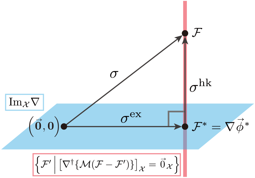
Figure 4: The geometric decomposition of the EPR for RDSs. Here, the blue plane indicates $\mathrm{Im}_{\mathcal{X}}\nabla$, and the red line indicates $\{\mathcal{F}^{\prime}|[\nabla^{{\dagger}}\{\mathcal{M}(\mathcal{F}-\mathcal{F}^{\prime})\}]_{\mathcal{X}}=\mathchoice{\overset{\smash{\lower 1.07639pt\hbox{\scalebox{0.45}{$\bm{\rightarrow}$}}}}{0}}{\overset{\smash{\lower 1.07639pt\hbox{\scalebox{0.45}{$\bm{\rightarrow}$}}}}{0}}{\overset{\smash{\lower 0.6458pt\hbox{\scalebox{0.3}{$\bm{\rightarrow}$}}}}{0}}{\overset{\smash{\lower 0.6458pt\hbox{\scalebox{0.3}{$\bm{\rightarrow}$}}}}{0}}_{\mathcal{X}}\}$. The thermodynamic force, whose squared norm is the EPR $\sigma=\left\llangle\mathcal{F},\mathcal{F}\right\rrangle_{\mathcal{M}}$, is decomposed into the two orthogonal parts: the projection of $\mathcal{F}$ onto $\mathrm{Im}_{\mathcal{X}}\nabla$, $\mathcal{F}^{\ast}$, whose squared norm is the excess EPR $\sigma^{\mathrm{ex}}=\left\llangle\mathcal{F}^{\ast},\mathcal{F}^{\ast}\right\rrangle_{\mathcal{M}}$, and the remaining part, $\mathcal{F}-\mathcal{F}^{\ast}$, whose squared norm is the housekeeping EPR $\sigma^{\mathrm{hk}}=\left\llangle\mathcal{F}-\mathcal{F}^{\ast},\mathcal{F}-\mathcal{F}^{\ast}\right\rrangle_{\mathcal{M}}$. This description is parallel to the case of the Langevin systems shown in Fig. 2.

The EPR $\sigma=\left\llangle\mathcal{F},\mathcal{F}\right\rrangle_{\mathcal{M}}$ includes contributions from both conservative and nonconservative sources, as shown in Eq. (99). To quantify these two contributions separately, we construct the geometric excess/housekeeping decomposition of EPR for RDSs by using the Pythagorean theorem

$$\left\llangle\mathcal{F},\mathcal{F}\right\rrangle_{\mathcal{M}}=\left\llangle\mathcal{F}^{\ast},\mathcal{F}^{\ast}\right\rrangle_{\mathcal{M}}+\left\llangle\mathcal{F}-\mathcal{F}^{\ast},\mathcal{F}-\mathcal{F}^{\ast}\right\rrangle_{\mathcal{M}}.$$ (101)

In the following, we show that choosing $\mathcal{F}^{\ast}$ to be the projection of the force onto the conservative force space allows us to use the Pythagorean theorem to decompose EPR into contributions from conservative and nonconservative forces, as in the case of Langevin systems (Sec. II.2). Here, we define the conservative force space as

$$\mathrm{Im}_{\mathcal{X}}\nabla\coloneqq\{\nabla\mathchoice{\kern-0.15pt\overset{\kern 0.7pt\smash{\lower 1.07639pt\hbox{\scalebox{0.45}{$\bm{\rightarrow}$}}}\kern-0.3pt}{\phi}}{\kern-0.15pt\overset{\kern 0.7pt\smash{\lower 1.07639pt\hbox{\scalebox{0.45}{$\bm{\rightarrow}$}}}\kern-0.3pt}{\phi}}{\overset{\smash{\lower 0.6458pt\hbox{\kern 0.2pt\scalebox{0.3}{$\bm{\rightarrow}$}\kern-0.8pt}}}{\phi}}{\overset{\smash{\lower 0.6458pt\hbox{\kern 0.2pt\scalebox{0.3}{$\bm{\rightarrow}$}\kern-0.8pt}}}{\phi}}\mid\forall\alpha\in\mathcal{Y},\,\phi_{\alpha}=0\}.$$ (102)

Here we use that conservative forces can be written as the generalized gradient of a potential whose external part is the zero vector, as discussed in Sec. III.5.

Projection of the force onto the conservative force space— We introduce the projected conservative force $\mathcal{F}^{\ast}$ as

$$\mathcal{F}^{\ast}\coloneqq\operatorname*{arg\,min}_{\mathcal{F}^{\prime}\in\mathrm{Im}_{\mathcal{X}}\nabla}\left\llangle\mathcal{F}-\mathcal{F}^{\prime},\mathcal{F}-\mathcal{F}^{\prime}\right\rrangle_{\mathcal{M}},$$ (103)

where we impose the same boundary condition on the diffusion part of $\mathcal{M}\mathcal{F}^{\prime}$ as we do on $\mathcal{J}=\mathcal{M}\mathcal{F}$. For example, if we consider a system with the no-flux boundary condition on the diffusion currents of the internal species, then we also impose the same condition on $(\overset{\smash{\lower 1.07639pt\hbox{\scalebox{0.7}[0.45]{$\bm{\leftrightarrow}$}}}}{\mathsf{M}}\mathchoice{\kern-0.15pt\overset{\kern 0.7pt\smash{\lower 1.07639pt\hbox{\scalebox{0.45}{$\bm{\rightarrow}$}}}\kern-0.3pt}{\bm{F}}}{\kern-0.15pt\overset{\kern 0.7pt\smash{\lower 1.07639pt\hbox{\scalebox{0.45}{$\bm{\rightarrow}$}}}\kern-0.3pt}{\bm{F}}}{\overset{\smash{\lower 0.6458pt\hbox{\kern 0.2pt\scalebox{0.3}{$\bm{\rightarrow}$}\kern-0.8pt}}}{\bm{F}}}{\overset{\smash{\lower 0.6458pt\hbox{\kern 0.2pt\scalebox{0.3}{$\bm{\rightarrow}$}\kern-0.8pt}}}{\bm{F}}}{}^{\prime})_{\mathcal{X}}$ in the minimization problem.

By definition, $\mathcal{F}^{\ast}$ can be given as $\mathcal{F}^{\ast}=\nabla\mathchoice{\kern-0.15pt\overset{\kern 0.7pt\smash{\lower 1.07639pt\hbox{\scalebox{0.45}{$\bm{\rightarrow}$}}}\kern-0.3pt}{\phi}}{\kern-0.15pt\overset{\kern 0.7pt\smash{\lower 1.07639pt\hbox{\scalebox{0.45}{$\bm{\rightarrow}$}}}\kern-0.3pt}{\phi}}{\overset{\smash{\lower 0.6458pt\hbox{\kern 0.2pt\scalebox{0.3}{$\bm{\rightarrow}$}\kern-0.8pt}}}{\phi}}{\overset{\smash{\lower 0.6458pt\hbox{\kern 0.2pt\scalebox{0.3}{$\bm{\rightarrow}$}\kern-0.8pt}}}{\phi}}{}^{\ast}$ with

$$\mathchoice{\kern-0.15pt\overset{\kern 0.7pt\smash{\lower 1.07639pt\hbox{\scalebox{0.45}{$\bm{\rightarrow}$}}}\kern-0.3pt}{\phi}}{\kern-0.15pt\overset{\kern 0.7pt\smash{\lower 1.07639pt\hbox{\scalebox{0.45}{$\bm{\rightarrow}$}}}\kern-0.3pt}{\phi}}{\overset{\smash{\lower 0.6458pt\hbox{\kern 0.2pt\scalebox{0.3}{$\bm{\rightarrow}$}\kern-0.8pt}}}{\phi}}{\overset{\smash{\lower 0.6458pt\hbox{\kern 0.2pt\scalebox{0.3}{$\bm{\rightarrow}$}\kern-0.8pt}}}{\phi}}{}^{\ast}\in\operatorname*{arg\,min}_{\mathchoice{\kern-0.15pt\overset{\kern 0.7pt\smash{\lower 0.75346pt\hbox{\scalebox{0.45}{$\bm{\rightarrow}$}}}\kern-0.3pt}{\phi}}{\kern-0.15pt\overset{\kern 0.7pt\smash{\lower 0.75346pt\hbox{\scalebox{0.45}{$\bm{\rightarrow}$}}}\kern-0.3pt}{\phi}}{\overset{\smash{\lower 0.45206pt\hbox{\kern 0.2pt\scalebox{0.3}{$\bm{\rightarrow}$}\kern-0.8pt}}}{\phi}}{\overset{\smash{\lower 0.45206pt\hbox{\kern 0.2pt\scalebox{0.3}{$\bm{\rightarrow}$}\kern-0.8pt}}}{\phi}}\mid\mathchoice{\kern-0.15pt\overset{\kern 0.7pt\smash{\lower 0.75346pt\hbox{\scalebox{0.45}{$\bm{\rightarrow}$}}}\kern-0.3pt}{\phi}}{\kern-0.15pt\overset{\kern 0.7pt\smash{\lower 0.75346pt\hbox{\scalebox{0.45}{$\bm{\rightarrow}$}}}\kern-0.3pt}{\phi}}{\overset{\smash{\lower 0.45206pt\hbox{\kern 0.2pt\scalebox{0.3}{$\bm{\rightarrow}$}\kern-0.8pt}}}{\phi}}{\overset{\smash{\lower 0.45206pt\hbox{\kern 0.2pt\scalebox{0.3}{$\bm{\rightarrow}$}\kern-0.8pt}}}{\phi}}_{\mathcal{Y}}=\mathchoice{\overset{\smash{\lower 0.75346pt\hbox{\scalebox{0.45}{$\bm{\rightarrow}$}}}}{0}}{\overset{\smash{\lower 0.75346pt\hbox{\scalebox{0.45}{$\bm{\rightarrow}$}}}}{0}}{\overset{\smash{\lower 0.45206pt\hbox{\scalebox{0.3}{$\bm{\rightarrow}$}}}}{0}}{\overset{\smash{\lower 0.45206pt\hbox{\scalebox{0.3}{$\bm{\rightarrow}$}}}}{0}}_{\mathcal{Y}}}\left\llangle\mathcal{F}-\nabla\mathchoice{\kern-0.15pt\overset{\kern 0.7pt\smash{\lower 1.07639pt\hbox{\scalebox{0.45}{$\bm{\rightarrow}$}}}\kern-0.3pt}{\phi}}{\kern-0.15pt\overset{\kern 0.7pt\smash{\lower 1.07639pt\hbox{\scalebox{0.45}{$\bm{\rightarrow}$}}}\kern-0.3pt}{\phi}}{\overset{\smash{\lower 0.6458pt\hbox{\kern 0.2pt\scalebox{0.3}{$\bm{\rightarrow}$}\kern-0.8pt}}}{\phi}}{\overset{\smash{\lower 0.6458pt\hbox{\kern 0.2pt\scalebox{0.3}{$\bm{\rightarrow}$}\kern-0.8pt}}}{\phi}},\mathcal{F}-\nabla\mathchoice{\kern-0.15pt\overset{\kern 0.7pt\smash{\lower 1.07639pt\hbox{\scalebox{0.45}{$\bm{\rightarrow}$}}}\kern-0.3pt}{\phi}}{\kern-0.15pt\overset{\kern 0.7pt\smash{\lower 1.07639pt\hbox{\scalebox{0.45}{$\bm{\rightarrow}$}}}\kern-0.3pt}{\phi}}{\overset{\smash{\lower 0.6458pt\hbox{\kern 0.2pt\scalebox{0.3}{$\bm{\rightarrow}$}\kern-0.8pt}}}{\phi}}{\overset{\smash{\lower 0.6458pt\hbox{\kern 0.2pt\scalebox{0.3}{$\bm{\rightarrow}$}\kern-0.8pt}}}{\phi}}\right\rrangle_{\mathcal{M}}.$$ (104)

Here, we also impose the same boundary condition on the diffusion part of $\mathcal{M}\nabla\mathchoice{\kern-0.15pt\overset{\kern 0.7pt\smash{\lower 1.07639pt\hbox{\scalebox{0.45}{$\bm{\rightarrow}$}}}\kern-0.3pt}{\phi}}{\kern-0.15pt\overset{\kern 0.7pt\smash{\lower 1.07639pt\hbox{\scalebox{0.45}{$\bm{\rightarrow}$}}}\kern-0.3pt}{\phi}}{\overset{\smash{\lower 0.6458pt\hbox{\kern 0.2pt\scalebox{0.3}{$\bm{\rightarrow}$}\kern-0.8pt}}}{\phi}}{\overset{\smash{\lower 0.6458pt\hbox{\kern 0.2pt\scalebox{0.3}{$\bm{\rightarrow}$}\kern-0.8pt}}}{\phi}}$ as we do on $\mathcal{J}=\mathcal{M}\mathcal{F}$ in the minimization problem. The minimization problem in Eq. (104) reduces to solving the partial differential equation

$$\quantity(\nabla^{{\dagger}}\mathcal{M}\mathcal{F})_{\mathcal{X}}=\quantity(\nabla^{{\dagger}}\mathcal{M}\nabla\mathchoice{\kern-0.15pt\overset{\kern 0.7pt\smash{\lower 1.07639pt\hbox{\scalebox{0.45}{$\bm{\rightarrow}$}}}\kern-0.3pt}{\phi}}{\kern-0.15pt\overset{\kern 0.7pt\smash{\lower 1.07639pt\hbox{\scalebox{0.45}{$\bm{\rightarrow}$}}}\kern-0.3pt}{\phi}}{\overset{\smash{\lower 0.6458pt\hbox{\kern 0.2pt\scalebox{0.3}{$\bm{\rightarrow}$}\kern-0.8pt}}}{\phi}}{\overset{\smash{\lower 0.6458pt\hbox{\kern 0.2pt\scalebox{0.3}{$\bm{\rightarrow}$}\kern-0.8pt}}}{\phi}}{}^{\ast})_{\mathcal{X}}$$ (105)

with the same boundary condition on $(\overset{\smash{\lower 1.07639pt\hbox{\scalebox{0.7}[0.45]{$\bm{\leftrightarrow}$}}}}{\mathsf{M}}\bm{\nabla}_{\bm{r}}\mathchoice{\kern-0.15pt\overset{\kern 0.7pt\smash{\lower 1.07639pt\hbox{\scalebox{0.45}{$\bm{\rightarrow}$}}}\kern-0.3pt}{\phi}}{\kern-0.15pt\overset{\kern 0.7pt\smash{\lower 1.07639pt\hbox{\scalebox{0.45}{$\bm{\rightarrow}$}}}\kern-0.3pt}{\phi}}{\overset{\smash{\lower 0.6458pt\hbox{\kern 0.2pt\scalebox{0.3}{$\bm{\rightarrow}$}\kern-0.8pt}}}{\phi}}{\overset{\smash{\lower 0.6458pt\hbox{\kern 0.2pt\scalebox{0.3}{$\bm{\rightarrow}$}\kern-0.8pt}}}{\phi}})_{\mathcal{X}}$ as we imposed on the original dynamics of internal species. Here, we obtain the partial differential equation in Eq. (105) as the Euler–Lagrange equation, and we can uniquely determine $\mathcal{F}^{\ast}$ (see Appendix B.1 for details).

The projected conservative force $\mathcal{F}^{\ast}=\nabla\mathchoice{\kern-0.15pt\overset{\kern 0.7pt\smash{\lower 1.07639pt\hbox{\scalebox{0.45}{$\bm{\rightarrow}$}}}\kern-0.3pt}{\phi}}{\kern-0.15pt\overset{\kern 0.7pt\smash{\lower 1.07639pt\hbox{\scalebox{0.45}{$\bm{\rightarrow}$}}}\kern-0.3pt}{\phi}}{\overset{\smash{\lower 0.6458pt\hbox{\kern 0.2pt\scalebox{0.3}{$\bm{\rightarrow}$}\kern-0.8pt}}}{\phi}}{\overset{\smash{\lower 0.6458pt\hbox{\kern 0.2pt\scalebox{0.3}{$\bm{\rightarrow}$}\kern-0.8pt}}}{\phi}}{}^{*}$ preserves the time evolution of the original dynamics of internal species because Eq. (105) provides the same time evolution of $\mathchoice{\kern-0.15pt\overset{\kern 0.7pt\smash{\lower 1.07639pt\hbox{\scalebox{0.45}{$\bm{\rightarrow}$}}}\kern-0.3pt}{c}}{\kern-0.15pt\overset{\kern 0.7pt\smash{\lower 1.07639pt\hbox{\scalebox{0.45}{$\bm{\rightarrow}$}}}\kern-0.3pt}{c}}{\overset{\smash{\lower 0.6458pt\hbox{\kern 0.2pt\scalebox{0.3}{$\bm{\rightarrow}$}\kern-0.8pt}}}{c}}{\overset{\smash{\lower 0.6458pt\hbox{\kern 0.2pt\scalebox{0.3}{$\bm{\rightarrow}$}\kern-0.8pt}}}{c}}_{\mathcal{X}}$:

$$\partial_{t}\mathchoice{\kern-0.15pt\overset{\kern 0.7pt\smash{\lower 1.07639pt\hbox{\scalebox{0.45}{$\bm{\rightarrow}$}}}\kern-0.3pt}{c}}{\kern-0.15pt\overset{\kern 0.7pt\smash{\lower 1.07639pt\hbox{\scalebox{0.45}{$\bm{\rightarrow}$}}}\kern-0.3pt}{c}}{\overset{\smash{\lower 0.6458pt\hbox{\kern 0.2pt\scalebox{0.3}{$\bm{\rightarrow}$}\kern-0.8pt}}}{c}}{\overset{\smash{\lower 0.6458pt\hbox{\kern 0.2pt\scalebox{0.3}{$\bm{\rightarrow}$}\kern-0.8pt}}}{c}}_{\mathcal{X}}=\quantity(\nabla^{{\dagger}}\mathcal{M}\mathcal{F})_{\mathcal{X}}=\quantity(\nabla^{{\dagger}}\mathcal{M}\nabla\mathchoice{\kern-0.15pt\overset{\kern 0.7pt\smash{\lower 1.07639pt\hbox{\scalebox{0.45}{$\bm{\rightarrow}$}}}\kern-0.3pt}{\phi}}{\kern-0.15pt\overset{\kern 0.7pt\smash{\lower 1.07639pt\hbox{\scalebox{0.45}{$\bm{\rightarrow}$}}}\kern-0.3pt}{\phi}}{\overset{\smash{\lower 0.6458pt\hbox{\kern 0.2pt\scalebox{0.3}{$\bm{\rightarrow}$}\kern-0.8pt}}}{\phi}}{\overset{\smash{\lower 0.6458pt\hbox{\kern 0.2pt\scalebox{0.3}{$\bm{\rightarrow}$}\kern-0.8pt}}}{\phi}}{}^{*})_{\mathcal{X}}.$$ (106)

From this dynamics-conservation viewpoint, we may come up with another representation of $\mathcal{F}^{\ast}$ as

$$\mathcal{F}^{\ast}=\operatorname*{arg\,min}_{\mathcal{F}^{\prime}|(\nabla^{{\dagger}}\mathcal{M}\mathcal{F}^{\prime})_{\mathcal{X}}=(\nabla^{{\dagger}}\mathcal{M}\mathcal{F})_{\mathcal{X}}}\left\llangle\mathcal{F}^{\prime},\mathcal{F}^{\prime}\right\rrangle_{\mathcal{M}},$$ (107)

with the same boundary condition as Eq. (103). We can actually check that the minimization problem in Eq. (107) leads to the same Euler–Lagrange equation as Eq. (105). Note that the potential $\mathchoice{\kern-0.15pt\overset{\kern 0.7pt\smash{\lower 1.07639pt\hbox{\scalebox{0.45}{$\bm{\rightarrow}$}}}\kern-0.3pt}{\phi}}{\kern-0.15pt\overset{\kern 0.7pt\smash{\lower 1.07639pt\hbox{\scalebox{0.45}{$\bm{\rightarrow}$}}}\kern-0.3pt}{\phi}}{\overset{\smash{\lower 0.6458pt\hbox{\kern 0.2pt\scalebox{0.3}{$\bm{\rightarrow}$}\kern-0.8pt}}}{\phi}}{\overset{\smash{\lower 0.6458pt\hbox{\kern 0.2pt\scalebox{0.3}{$\bm{\rightarrow}$}\kern-0.8pt}}}{\phi}}$, whose external part is the zero vector, is introduced as the Lagrange multiplier for the constraint $(\nabla^{{\dagger}}\mathcal{M}\mathcal{F}^{\prime})_{\mathcal{X}}=(\nabla^{{\dagger}}\mathcal{M}\mathcal{F})_{\mathcal{X}}$ in Eq. (107) (see Appendix B.2).

The projected conservative force $\mathcal{F}^{\ast}$ is orthogonal to $\mathcal{F}-\mathcal{F}^{\ast}$ with respect to the inner product $\left\llangle\cdot,\cdot\right\rrangle_{\mathcal{M}}$ as

$$\left\llangle\mathcal{F}-\mathcal{F}^{\ast},\mathcal{F}^{\ast}\right\rrangle_{\mathcal{M}} =\left\llangle\mathcal{M}\quantity(\mathcal{F}-\mathcal{F}^{\ast}),\nabla\mathchoice{\kern-0.15pt\overset{\kern 0.7pt\smash{\lower 1.07639pt\hbox{\scalebox{0.45}{$\bm{\rightarrow}$}}}\kern-0.3pt}{\phi}}{\kern-0.15pt\overset{\kern 0.7pt\smash{\lower 1.07639pt\hbox{\scalebox{0.45}{$\bm{\rightarrow}$}}}\kern-0.3pt}{\phi}}{\overset{\smash{\lower 0.6458pt\hbox{\kern 0.2pt\scalebox{0.3}{$\bm{\rightarrow}$}\kern-0.8pt}}}{\phi}}{\overset{\smash{\lower 0.6458pt\hbox{\kern 0.2pt\scalebox{0.3}{$\bm{\rightarrow}$}\kern-0.8pt}}}{\phi}}{}^{\ast}\right\rrangle$$

$$=\left\langle\nabla^{{\dagger}}\mathcal{M}\quantity(\mathcal{F}-\mathcal{F}^{\ast}),\mathchoice{\kern-0.15pt\overset{\kern 0.7pt\smash{\lower 1.07639pt\hbox{\scalebox{0.45}{$\bm{\rightarrow}$}}}\kern-0.3pt}{\phi}}{\kern-0.15pt\overset{\kern 0.7pt\smash{\lower 1.07639pt\hbox{\scalebox{0.45}{$\bm{\rightarrow}$}}}\kern-0.3pt}{\phi}}{\overset{\smash{\lower 0.6458pt\hbox{\kern 0.2pt\scalebox{0.3}{$\bm{\rightarrow}$}\kern-0.8pt}}}{\phi}}{\overset{\smash{\lower 0.6458pt\hbox{\kern 0.2pt\scalebox{0.3}{$\bm{\rightarrow}$}\kern-0.8pt}}}{\phi}}{}^{\ast}\right\rangle$$

$$=0,$$ (108)

Here, we used the boundary condition on $(\mathcal{M}\nabla\mathchoice{\kern-0.15pt\overset{\kern 0.7pt\smash{\lower 1.07639pt\hbox{\scalebox{0.45}{$\bm{\rightarrow}$}}}\kern-0.3pt}{\phi}}{\kern-0.15pt\overset{\kern 0.7pt\smash{\lower 1.07639pt\hbox{\scalebox{0.45}{$\bm{\rightarrow}$}}}\kern-0.3pt}{\phi}}{\overset{\smash{\lower 0.6458pt\hbox{\kern 0.2pt\scalebox{0.3}{$\bm{\rightarrow}$}\kern-0.8pt}}}{\phi}}{\overset{\smash{\lower 0.6458pt\hbox{\kern 0.2pt\scalebox{0.3}{$\bm{\rightarrow}$}\kern-0.8pt}}}{\phi}}{}^{\ast})_{\mathcal{X}}$, the condition that $\phi^{\ast}_{\alpha}=0$ for all $\alpha\in\mathcal{Y}$, and Eq. (82) in the second transformation. We also used the condition that $\phi^{\ast}_{\alpha}=0$ for all $\alpha\in\mathcal{Y}$ and the Euler–Lagrange equation (105) in the third transformation. This orthogonality finally leads to the Pythagorean theorem [Eq. (101)], which enables us to define a decomposition of the EPR.

Excess/housekeeping decomposition of EPR— We define the excess and housekeeping EPRs (see also Fig.4) as

$$\sigma^{\mathrm{ex}}\coloneqq\left\llangle\mathcal{F}^{\ast},\mathcal{F}^{\ast}\right\rrangle_{\mathcal{M}},\;\sigma^{\mathrm{hk}}\coloneqq\left\llangle\mathcal{F}-\mathcal{F}^{\ast},\mathcal{F}-\mathcal{F}^{\ast}\right\rrangle_{\mathcal{M}}.$$ (109)

The excess and housekeeping EPRs are nonnegative because they are represented by a squared norm. The Pythagorean theorem [Eq. (101)] and $\sigma=\left\llangle\mathcal{F},\mathcal{F}\right\rrangle_{\mathcal{M}}$ [Eq. (90)] show that the excess and housekeeping EPRs give the decomposition of the EPR into two nonnegative parts as

$$\sigma=\sigma^{\mathrm{ex}}+\sigma^{\mathrm{hk}}.$$ (110)

Time integration of Eq. (110) leads to the geometric excess/housekeeping decomposition of the EP as

$$\Sigma_{\tau}=\Sigma^{\mathrm{ex}}_{\tau}+\Sigma^{\mathrm{hk}}_{\tau}.$$ (111)

The minimization problems, Eq. (103) and Eq. (107), mean the excess EPR $\sigma_{\mathrm{ex}}$ is the minimum dissipation by the conservative force required to achieve the original dynamics of the internal species. Indeed, the excess EPR is given by the following optimization problem,

$$\sigma^{\mathrm{ex}}=\inf_{\mathcal{F}^{\prime}|(\nabla^{{\dagger}}\mathcal{M}\mathcal{F}^{\prime})_{\mathcal{X}}=(\nabla^{{\dagger}}\mathcal{M}\mathcal{F})_{\mathcal{X}}}\left\llangle\mathcal{F}^{\prime},\mathcal{F}^{\prime}\right\rrangle_{\mathcal{M}}.$$ (112)

Here, we also impose the same boundary condition on $\mathcal{M}\mathcal{F}^{\prime}$ as Eq. (103). The form of $\mathcal{F}^{\ast}$ in Eq. (107) shows that the excess EPR vanishes at the steady state when the system is closed because the zero function $\mathcal{F}^{\ast}=(\mathchoice{\kern-0.15pt\overset{\kern 0.7pt\smash{\lower 1.07639pt\hbox{\scalebox{0.45}{$\bm{\rightarrow}$}}}\kern-0.3pt}{\bm{0}}}{\kern-0.15pt\overset{\kern 0.7pt\smash{\lower 1.07639pt\hbox{\scalebox{0.45}{$\bm{\rightarrow}$}}}\kern-0.3pt}{\bm{0}}}{\overset{\smash{\lower 0.6458pt\hbox{\kern 0.2pt\scalebox{0.3}{$\bm{\rightarrow}$}\kern-0.8pt}}}{\bm{0}}}{\overset{\smash{\lower 0.6458pt\hbox{\kern 0.2pt\scalebox{0.3}{$\bm{\rightarrow}$}\kern-0.8pt}}}{\bm{0}}},\bm{0})$ satisfies the constraints. If the system is open, the excess EPR will be zero as long as the concentrations of the internal species are stationary, even if those of the external species may not be. We remark that we can rewrite $\sigma^{\mathrm{ex}}$ as the time derivative of a quantity in relation to the conservative forces that drive relaxation [40] (see also Appendix C).

The housekeeping EPR $\sigma^{\mathrm{hk}}$ is also given by the following optimization problem,

$$\sigma^{\mathrm{hk}} =\inf_{\mathcal{F}^{\prime}\in\mathrm{Im}_{\mathcal{X}}\nabla}\left\llangle\mathcal{F}-\mathcal{F}^{\prime},\mathcal{F}-\mathcal{F}^{\prime}\right\rrangle_{\mathcal{M}}$$

$$=\inf_{\mathchoice{\kern-0.15pt\overset{\kern 0.7pt\smash{\lower 0.75346pt\hbox{\scalebox{0.45}{$\bm{\rightarrow}$}}}\kern-0.3pt}{\phi}}{\kern-0.15pt\overset{\kern 0.7pt\smash{\lower 0.75346pt\hbox{\scalebox{0.45}{$\bm{\rightarrow}$}}}\kern-0.3pt}{\phi}}{\overset{\smash{\lower 0.45206pt\hbox{\kern 0.2pt\scalebox{0.3}{$\bm{\rightarrow}$}\kern-0.8pt}}}{\phi}}{\overset{\smash{\lower 0.45206pt\hbox{\kern 0.2pt\scalebox{0.3}{$\bm{\rightarrow}$}\kern-0.8pt}}}{\phi}}|\mathchoice{\kern-0.15pt\overset{\kern 0.7pt\smash{\lower 0.75346pt\hbox{\scalebox{0.45}{$\bm{\rightarrow}$}}}\kern-0.3pt}{\phi}}{\kern-0.15pt\overset{\kern 0.7pt\smash{\lower 0.75346pt\hbox{\scalebox{0.45}{$\bm{\rightarrow}$}}}\kern-0.3pt}{\phi}}{\overset{\smash{\lower 0.45206pt\hbox{\kern 0.2pt\scalebox{0.3}{$\bm{\rightarrow}$}\kern-0.8pt}}}{\phi}}{\overset{\smash{\lower 0.45206pt\hbox{\kern 0.2pt\scalebox{0.3}{$\bm{\rightarrow}$}\kern-0.8pt}}}{\phi}}_{\mathcal{Y}}=\mathchoice{\overset{\smash{\lower 0.75346pt\hbox{\scalebox{0.45}{$\bm{\rightarrow}$}}}}{0}}{\overset{\smash{\lower 0.75346pt\hbox{\scalebox{0.45}{$\bm{\rightarrow}$}}}}{0}}{\overset{\smash{\lower 0.45206pt\hbox{\scalebox{0.3}{$\bm{\rightarrow}$}}}}{0}}{\overset{\smash{\lower 0.45206pt\hbox{\scalebox{0.3}{$\bm{\rightarrow}$}}}}{0}}_{\mathcal{Y}}}\left\llangle\mathcal{F}-\nabla\mathchoice{\kern-0.15pt\overset{\kern 0.7pt\smash{\lower 1.07639pt\hbox{\scalebox{0.45}{$\bm{\rightarrow}$}}}\kern-0.3pt}{\phi}}{\kern-0.15pt\overset{\kern 0.7pt\smash{\lower 1.07639pt\hbox{\scalebox{0.45}{$\bm{\rightarrow}$}}}\kern-0.3pt}{\phi}}{\overset{\smash{\lower 0.6458pt\hbox{\kern 0.2pt\scalebox{0.3}{$\bm{\rightarrow}$}\kern-0.8pt}}}{\phi}}{\overset{\smash{\lower 0.6458pt\hbox{\kern 0.2pt\scalebox{0.3}{$\bm{\rightarrow}$}\kern-0.8pt}}}{\phi}},\mathcal{F}-\nabla\mathchoice{\kern-0.15pt\overset{\kern 0.7pt\smash{\lower 1.07639pt\hbox{\scalebox{0.45}{$\bm{\rightarrow}$}}}\kern-0.3pt}{\phi}}{\kern-0.15pt\overset{\kern 0.7pt\smash{\lower 1.07639pt\hbox{\scalebox{0.45}{$\bm{\rightarrow}$}}}\kern-0.3pt}{\phi}}{\overset{\smash{\lower 0.6458pt\hbox{\kern 0.2pt\scalebox{0.3}{$\bm{\rightarrow}$}\kern-0.8pt}}}{\phi}}{\overset{\smash{\lower 0.6458pt\hbox{\kern 0.2pt\scalebox{0.3}{$\bm{\rightarrow}$}\kern-0.8pt}}}{\phi}}\right\rrangle_{\mathcal{M}}.$$ (113)

Defining $\mathcal{J}^{\ast}=\mathcal{M}\mathcal{F}^{\ast}$, we can rewrite the Euler–Lagrange equation (105) as

$$\quantity(\nabla^{{\dagger}}\mathcal{J})_{\mathcal{X}}=\quantity(\nabla^{{\dagger}}\mathcal{J}^{\ast})_{\mathcal{X}}.$$ (114)

Therefore, $\mathcal{J}-\mathcal{J}^{\ast}\in{\mathrm{Ker}}_{\mathcal{X}}\nabla^{{\dagger}}$ holds, where $\mathrm{Ker}_{\mathcal{X}}\nabla^{{\dagger}}\coloneqq\{\mathcal{J}^{\prime}\mid\forall\alpha\in\mathcal{X},\;(\nabla^{{\dagger}}\mathcal{J}^{\prime})_{\alpha}=0\}$ is the set of cyclic currents. Such currents do not affect the dynamics of the internal species because

$$\partial_{t}\mathchoice{\kern-0.15pt\overset{\kern 0.7pt\smash{\lower 1.07639pt\hbox{\scalebox{0.45}{$\bm{\rightarrow}$}}}\kern-0.3pt}{c}}{\kern-0.15pt\overset{\kern 0.7pt\smash{\lower 1.07639pt\hbox{\scalebox{0.45}{$\bm{\rightarrow}$}}}\kern-0.3pt}{c}}{\overset{\smash{\lower 0.6458pt\hbox{\kern 0.2pt\scalebox{0.3}{$\bm{\rightarrow}$}\kern-0.8pt}}}{c}}{\overset{\smash{\lower 0.6458pt\hbox{\kern 0.2pt\scalebox{0.3}{$\bm{\rightarrow}$}\kern-0.8pt}}}{c}}_{\mathcal{X}}=\quantity(\nabla^{{\dagger}}\mathcal{J}^{*})_{\mathcal{X}}+\quantity(\nabla^{{\dagger}}\quantity[\mathcal{J}-\mathcal{J}^{*}])_{\mathcal{X}}=\quantity(\nabla^{{\dagger}}\mathcal{J}^{*})_{\mathcal{X}}.$$ (115)

Thus, the housekeeping EPR $\sigma^{\mathrm{hk}}$ is regarded as the dissipation due to cyclic currents that do not change the concentrations of the internal species. Note that the cyclic current $\mathcal{J}-\mathcal{J}^{\ast}$ can affect the concentrations of the external species because

$$\partial_{t}\mathchoice{\kern-0.15pt\overset{\kern 0.7pt\smash{\lower 1.07639pt\hbox{\scalebox{0.45}{$\bm{\rightarrow}$}}}\kern-0.3pt}{c}}{\kern-0.15pt\overset{\kern 0.7pt\smash{\lower 1.07639pt\hbox{\scalebox{0.45}{$\bm{\rightarrow}$}}}\kern-0.3pt}{c}}{\overset{\smash{\lower 0.6458pt\hbox{\kern 0.2pt\scalebox{0.3}{$\bm{\rightarrow}$}\kern-0.8pt}}}{c}}{\overset{\smash{\lower 0.6458pt\hbox{\kern 0.2pt\scalebox{0.3}{$\bm{\rightarrow}$}\kern-0.8pt}}}{c}}_{\mathcal{Y}} =\quantity(\nabla^{{\dagger}}\mathcal{J}^{*})_{\mathcal{Y}}+\quantity(\nabla^{{\dagger}}\quantity[\mathcal{J}-\mathcal{J}^{*}])_{\mathcal{Y}}$$ (116)

and the second term on the right-hand side does not vanish generally.

In other words, the housekeeping EPR consists of the cyclic contribution plus the contribution from the diffusion of external species. Suppose that the mobility tensor has no direct interaction terms between internal and external species, $\mathsf{M}_{(\alpha,\beta)}=\mathsf{O}$ if $(\alpha,\beta)\in\mathcal{X}\times\mathcal{Y}$ or $\mathcal{Y}\times\mathcal{X}$, where $\mathsf{O}$ is the zero matrix. Then, the interpretation is clearly depicted by the decomposition

$$\sigma^{\mathrm{hk}} =\sigma_{\mathcal{X}}^{\mathrm{cyc}}+\sigma_{\mathcal{Y}}^{\mathrm{diff}},$$ (117)

$$\sigma_{\mathcal{X}}^{\mathrm{cyc}} \coloneqq\int_{V}d\bm{r}\left[(\bm{f}-\nabla_{\mathsf{s}}\mathchoice{\kern-0.15pt\overset{\kern 0.7pt\smash{\lower 1.07639pt\hbox{\scalebox{0.45}{$\bm{\rightarrow}$}}}\kern-0.3pt}{\phi}}{\kern-0.15pt\overset{\kern 0.7pt\smash{\lower 1.07639pt\hbox{\scalebox{0.45}{$\bm{\rightarrow}$}}}\kern-0.3pt}{\phi}}{\overset{\smash{\lower 0.6458pt\hbox{\kern 0.2pt\scalebox{0.3}{$\bm{\rightarrow}$}\kern-0.8pt}}}{\phi}}{\overset{\smash{\lower 0.6458pt\hbox{\kern 0.2pt\scalebox{0.3}{$\bm{\rightarrow}$}\kern-0.8pt}}}{\phi}}{}^{\ast})^{\top}\mathsf{m}(\bm{f}-\nabla_{\mathsf{s}}\mathchoice{\kern-0.15pt\overset{\kern 0.7pt\smash{\lower 1.07639pt\hbox{\scalebox{0.45}{$\bm{\rightarrow}$}}}\kern-0.3pt}{\phi}}{\kern-0.15pt\overset{\kern 0.7pt\smash{\lower 1.07639pt\hbox{\scalebox{0.45}{$\bm{\rightarrow}$}}}\kern-0.3pt}{\phi}}{\overset{\smash{\lower 0.6458pt\hbox{\kern 0.2pt\scalebox{0.3}{$\bm{\rightarrow}$}\kern-0.8pt}}}{\phi}}{\overset{\smash{\lower 0.6458pt\hbox{\kern 0.2pt\scalebox{0.3}{$\bm{\rightarrow}$}\kern-0.8pt}}}{\phi}}{}^{\ast})\phantom{\sum_{\alpha,\beta\in\mathcal{X}}}\right.$$

$$\left.+\sum_{\alpha,\beta\in\mathcal{X}}(\bm{F}_{(\alpha)}-\bm{\nabla}_{\bm{r}}\phi_{\alpha}^{\ast})^{\top}\mathsf{M}_{(\alpha\beta)}(\bm{F}_{(\beta)}-\bm{\nabla}_{\bm{r}}\phi_{\beta}^{\ast})\right]\geq 0$$ (118)

$$\sigma_{\mathcal{Y}}^{\mathrm{diff}} \coloneqq\int_{V}d\bm{r}\sum_{\alpha\in\mathcal{Y}}\bm{J}_{(\alpha)}\cdot\bm{F}_{(\alpha)}\geq 0.$$ (119)

The first term $\sigma_{\mathcal{X}}^{\mathrm{cyc}}$ reflects the cyclic motion of the internal species, as arising from the cyclic current $\mathcal{J}-\mathcal{J}^{\ast}$. On the other hand, the remainder is given by the dissipation stemming only from the diffusion of the external species. This term is particular to RDSs, as the housekeeping EPR in a homogeneous CRN can be written only with cyclic contributions [40]. The decomposition is straightforwardly proved using the definition of $\sigma^{\mathrm{hk}}$ and the fact that $\bm{F}_{(\alpha)}-\bm{\nabla}_{\bm{r}}\phi^{*}_{\alpha}=\bm{F}_{(\alpha)}$ for any $\alpha\in\mathcal{Y}$ because $\phi_{\alpha}^{\ast}=0$ for any $\alpha\in\mathcal{Y}$ with the assumption $\mathsf{M}_{(\alpha,\beta)}=\mathsf{O}$ if $(\alpha,\beta)\in\mathcal{X}\times\mathcal{Y}$ or $\mathcal{Y}\times\mathcal{X}$.

It is worth noting that while the cyclic currents are cyclic in terms of internal species, they are caused by external factors in physics terms, such as external species or external nonconservative forces. This is also the case with homogeneous CRNs without detailed balance, where external species are often made implicit. If no such species exist, the system will be detailed balanced, and no cyclic motion will be observed.

IV.2 Local decomposition and wavenumber decomposition of entropy production rate

In this section, we discuss the local and wavenumber decomposition of EPR for RDSs, analogous to the decomposition for Langevin systems from Sec. II.3. The local and wavenumber EPRs enable us to quantify the dissipation at each point in the real and wavenumber spaces, respectively. Thus, we can detect local dissipation due to pattern formation via the local and wavenumber EPRs for RDSs. Further below, we use local EPR decomposition to quantify the spatial dissipation in numerical examples of pattern formation.

Local decomposition—We define the local EPR at the position $\bm{r}$ as

$$\sigma_{t}^{\mathrm{loc}}(\bm{r})\coloneqq\mathchoice{\kern-0.15pt\overset{\kern 0.7pt\smash{\lower 1.07639pt\hbox{\scalebox{0.45}{$\bm{\rightarrow}$}}}\kern-0.3pt}{\bm{J}}}{\kern-0.15pt\overset{\kern 0.7pt\smash{\lower 1.07639pt\hbox{\scalebox{0.45}{$\bm{\rightarrow}$}}}\kern-0.3pt}{\bm{J}}}{\overset{\smash{\lower 0.6458pt\hbox{\kern 0.2pt\scalebox{0.3}{$\bm{\rightarrow}$}\kern-0.8pt}}}{\bm{J}}}{\overset{\smash{\lower 0.6458pt\hbox{\kern 0.2pt\scalebox{0.3}{$\bm{\rightarrow}$}\kern-0.8pt}}}{\bm{J}}}{}^{\top}(\bm{r};t)\mathchoice{\kern-0.15pt\overset{\kern 0.7pt\smash{\lower 1.07639pt\hbox{\scalebox{0.45}{$\bm{\rightarrow}$}}}\kern-0.3pt}{\bm{F}}}{\kern-0.15pt\overset{\kern 0.7pt\smash{\lower 1.07639pt\hbox{\scalebox{0.45}{$\bm{\rightarrow}$}}}\kern-0.3pt}{\bm{F}}}{\overset{\smash{\lower 0.6458pt\hbox{\kern 0.2pt\scalebox{0.3}{$\bm{\rightarrow}$}\kern-0.8pt}}}{\bm{F}}}{\overset{\smash{\lower 0.6458pt\hbox{\kern 0.2pt\scalebox{0.3}{$\bm{\rightarrow}$}\kern-0.8pt}}}{\bm{F}}}(\bm{r};t)+\bm{j}^{\top}(\bm{r};t)\bm{f}(\bm{r};t).$$ (120)

The nonnegativity $\sigma_{t}^{\mathrm{loc}}(\bm{r})\geq 0$ holds locally as it is locally that $\overset{\smash{\lower 1.07639pt\hbox{\scalebox{0.7}[0.45]{$\bm{\leftrightarrow}$}}}}{\mathsf{M}}$ is assumed to be positive-definite and $\bm{j}$ and $\bm{f}$ have the same sign. The volume integral gives the EPR,

$$\sigma_{t}=\int_{V}d\bm{r}\sigma_{t}^{\mathrm{loc}}(\bm{r}).$$ (121)

This equality [Eq. (121)] indicates a decomposition of the EPR into the local EPRs, the dissipation at each location.

We also define the local excess and housekeeping EPRs at position $\bm{r}$ as

$$\sigma_{t}^{\mathrm{ex},\mathrm{loc}}(\bm{r})\coloneqq\quantity(\bm{\nabla}_{\bm{r}}\mathchoice{\kern-0.15pt\overset{\kern 0.7pt\smash{\lower 1.07639pt\hbox{\scalebox{0.45}{$\bm{\rightarrow}$}}}\kern-0.3pt}{\phi}}{\kern-0.15pt\overset{\kern 0.7pt\smash{\lower 1.07639pt\hbox{\scalebox{0.45}{$\bm{\rightarrow}$}}}\kern-0.3pt}{\phi}}{\overset{\smash{\lower 0.6458pt\hbox{\kern 0.2pt\scalebox{0.3}{$\bm{\rightarrow}$}\kern-0.8pt}}}{\phi}}{\overset{\smash{\lower 0.6458pt\hbox{\kern 0.2pt\scalebox{0.3}{$\bm{\rightarrow}$}\kern-0.8pt}}}{\phi}}{}^{\ast}){}^{\top}\overset{\smash{\lower 1.07639pt\hbox{\scalebox{0.7}[0.45]{$\bm{\leftrightarrow}$}}}}{\mathsf{M}}\bm{\nabla}_{\bm{r}}\mathchoice{\kern-0.15pt\overset{\kern 0.7pt\smash{\lower 1.07639pt\hbox{\scalebox{0.45}{$\bm{\rightarrow}$}}}\kern-0.3pt}{\phi}}{\kern-0.15pt\overset{\kern 0.7pt\smash{\lower 1.07639pt\hbox{\scalebox{0.45}{$\bm{\rightarrow}$}}}\kern-0.3pt}{\phi}}{\overset{\smash{\lower 0.6458pt\hbox{\kern 0.2pt\scalebox{0.3}{$\bm{\rightarrow}$}\kern-0.8pt}}}{\phi}}{\overset{\smash{\lower 0.6458pt\hbox{\kern 0.2pt\scalebox{0.3}{$\bm{\rightarrow}$}\kern-0.8pt}}}{\phi}}{}^{\ast}+\quantity(\nabla_{\mathsf{s}}\mathchoice{\kern-0.15pt\overset{\kern 0.7pt\smash{\lower 1.07639pt\hbox{\scalebox{0.45}{$\bm{\rightarrow}$}}}\kern-0.3pt}{\phi}}{\kern-0.15pt\overset{\kern 0.7pt\smash{\lower 1.07639pt\hbox{\scalebox{0.45}{$\bm{\rightarrow}$}}}\kern-0.3pt}{\phi}}{\overset{\smash{\lower 0.6458pt\hbox{\kern 0.2pt\scalebox{0.3}{$\bm{\rightarrow}$}\kern-0.8pt}}}{\phi}}{\overset{\smash{\lower 0.6458pt\hbox{\kern 0.2pt\scalebox{0.3}{$\bm{\rightarrow}$}\kern-0.8pt}}}{\phi}}{}^{\ast}){}^{\top}\mathsf{m}\nabla_{\mathsf{s}}\mathchoice{\kern-0.15pt\overset{\kern 0.7pt\smash{\lower 1.07639pt\hbox{\scalebox{0.45}{$\bm{\rightarrow}$}}}\kern-0.3pt}{\phi}}{\kern-0.15pt\overset{\kern 0.7pt\smash{\lower 1.07639pt\hbox{\scalebox{0.45}{$\bm{\rightarrow}$}}}\kern-0.3pt}{\phi}}{\overset{\smash{\lower 0.6458pt\hbox{\kern 0.2pt\scalebox{0.3}{$\bm{\rightarrow}$}\kern-0.8pt}}}{\phi}}{\overset{\smash{\lower 0.6458pt\hbox{\kern 0.2pt\scalebox{0.3}{$\bm{\rightarrow}$}\kern-0.8pt}}}{\phi}}{}^{\ast},$$ (122)

and

$$\sigma_{t}^{\mathrm{hk},\mathrm{loc}}(\bm{r})\coloneqq \quantity(\mathchoice{\kern-0.15pt\overset{\kern 0.7pt\smash{\lower 1.07639pt\hbox{\scalebox{0.45}{$\bm{\rightarrow}$}}}\kern-0.3pt}{\bm{F}}}{\kern-0.15pt\overset{\kern 0.7pt\smash{\lower 1.07639pt\hbox{\scalebox{0.45}{$\bm{\rightarrow}$}}}\kern-0.3pt}{\bm{F}}}{\overset{\smash{\lower 0.6458pt\hbox{\kern 0.2pt\scalebox{0.3}{$\bm{\rightarrow}$}\kern-0.8pt}}}{\bm{F}}}{\overset{\smash{\lower 0.6458pt\hbox{\kern 0.2pt\scalebox{0.3}{$\bm{\rightarrow}$}\kern-0.8pt}}}{\bm{F}}}-\bm{\nabla}_{\bm{r}}\mathchoice{\kern-0.15pt\overset{\kern 0.7pt\smash{\lower 1.07639pt\hbox{\scalebox{0.45}{$\bm{\rightarrow}$}}}\kern-0.3pt}{\phi}}{\kern-0.15pt\overset{\kern 0.7pt\smash{\lower 1.07639pt\hbox{\scalebox{0.45}{$\bm{\rightarrow}$}}}\kern-0.3pt}{\phi}}{\overset{\smash{\lower 0.6458pt\hbox{\kern 0.2pt\scalebox{0.3}{$\bm{\rightarrow}$}\kern-0.8pt}}}{\phi}}{\overset{\smash{\lower 0.6458pt\hbox{\kern 0.2pt\scalebox{0.3}{$\bm{\rightarrow}$}\kern-0.8pt}}}{\phi}}{}^{\ast}){}^{\top}\overset{\smash{\lower 1.07639pt\hbox{\scalebox{0.7}[0.45]{$\bm{\leftrightarrow}$}}}}{\mathsf{M}}\quantity(\mathchoice{\kern-0.15pt\overset{\kern 0.7pt\smash{\lower 1.07639pt\hbox{\scalebox{0.45}{$\bm{\rightarrow}$}}}\kern-0.3pt}{\bm{F}}}{\kern-0.15pt\overset{\kern 0.7pt\smash{\lower 1.07639pt\hbox{\scalebox{0.45}{$\bm{\rightarrow}$}}}\kern-0.3pt}{\bm{F}}}{\overset{\smash{\lower 0.6458pt\hbox{\kern 0.2pt\scalebox{0.3}{$\bm{\rightarrow}$}\kern-0.8pt}}}{\bm{F}}}{\overset{\smash{\lower 0.6458pt\hbox{\kern 0.2pt\scalebox{0.3}{$\bm{\rightarrow}$}\kern-0.8pt}}}{\bm{F}}}-\bm{\nabla}_{\bm{r}}\mathchoice{\kern-0.15pt\overset{\kern 0.7pt\smash{\lower 1.07639pt\hbox{\scalebox{0.45}{$\bm{\rightarrow}$}}}\kern-0.3pt}{\phi}}{\kern-0.15pt\overset{\kern 0.7pt\smash{\lower 1.07639pt\hbox{\scalebox{0.45}{$\bm{\rightarrow}$}}}\kern-0.3pt}{\phi}}{\overset{\smash{\lower 0.6458pt\hbox{\kern 0.2pt\scalebox{0.3}{$\bm{\rightarrow}$}\kern-0.8pt}}}{\phi}}{\overset{\smash{\lower 0.6458pt\hbox{\kern 0.2pt\scalebox{0.3}{$\bm{\rightarrow}$}\kern-0.8pt}}}{\phi}}{}^{\ast})$$

$$+\quantity(\bm{f}-\nabla_{\mathsf{s}}\mathchoice{\kern-0.15pt\overset{\kern 0.7pt\smash{\lower 1.07639pt\hbox{\scalebox{0.45}{$\bm{\rightarrow}$}}}\kern-0.3pt}{\phi}}{\kern-0.15pt\overset{\kern 0.7pt\smash{\lower 1.07639pt\hbox{\scalebox{0.45}{$\bm{\rightarrow}$}}}\kern-0.3pt}{\phi}}{\overset{\smash{\lower 0.6458pt\hbox{\kern 0.2pt\scalebox{0.3}{$\bm{\rightarrow}$}\kern-0.8pt}}}{\phi}}{\overset{\smash{\lower 0.6458pt\hbox{\kern 0.2pt\scalebox{0.3}{$\bm{\rightarrow}$}\kern-0.8pt}}}{\phi}}{}^{\ast}){}^{\top}\mathsf{m}\quantity(\bm{f}-\nabla_{\mathsf{s}}\mathchoice{\kern-0.15pt\overset{\kern 0.7pt\smash{\lower 1.07639pt\hbox{\scalebox{0.45}{$\bm{\rightarrow}$}}}\kern-0.3pt}{\phi}}{\kern-0.15pt\overset{\kern 0.7pt\smash{\lower 1.07639pt\hbox{\scalebox{0.45}{$\bm{\rightarrow}$}}}\kern-0.3pt}{\phi}}{\overset{\smash{\lower 0.6458pt\hbox{\kern 0.2pt\scalebox{0.3}{$\bm{\rightarrow}$}\kern-0.8pt}}}{\phi}}{\overset{\smash{\lower 0.6458pt\hbox{\kern 0.2pt\scalebox{0.3}{$\bm{\rightarrow}$}\kern-0.8pt}}}{\phi}}{}^{\ast}),$$ (123)

which satisfy $\int_{V}d\bm{r}\sigma_{t}^{\mathrm{ex},\mathrm{loc}}(\bm{r})=\sigma^{\mathrm{ex}}_{t}$ and $\int_{V}d\bm{r}\sigma_{t}^{\mathrm{hk},\mathrm{loc}}(\bm{r})=\sigma^{\mathrm{hk}}_{t}$. The local excess and housekeeping EPRs are nonnegative because $\overset{\smash{\lower 1.07639pt\hbox{\scalebox{0.7}[0.45]{$\bm{\leftrightarrow}$}}}}{\mathsf{M}}$ and $\mathsf{m}$ are positive-definite. Thus, we can interpret $\sigma_{t}^{\mathrm{ex,loc}}(\bm{r})$ as entropy production rate due to the projected conservative force $\mathcal{F}^{\ast}$ at the location $\bm{r}$. We also can regard $\sigma_{t}^{\mathrm{hk,loc}}(\bm{r})$ as entropy production rate due to the cyclic current at the location $\bm{r}$. Note that $\sigma_{t}^{\mathrm{ex},\mathrm{loc}}(\bm{r})=0$ and $\sigma_{t}^{\mathrm{hk},\mathrm{loc}}(\bm{r})=\sigma_{t}^{\mathrm{loc}}(\bm{r})$ hold for all $\bm{r}\in V$ if and only if $\nabla\mathchoice{\kern-0.15pt\overset{\kern 0.7pt\smash{\lower 1.07639pt\hbox{\scalebox{0.45}{$\bm{\rightarrow}$}}}\kern-0.3pt}{\phi}}{\kern-0.15pt\overset{\kern 0.7pt\smash{\lower 1.07639pt\hbox{\scalebox{0.45}{$\bm{\rightarrow}$}}}\kern-0.3pt}{\phi}}{\overset{\smash{\lower 0.6458pt\hbox{\kern 0.2pt\scalebox{0.3}{$\bm{\rightarrow}$}\kern-0.8pt}}}{\phi}}{\overset{\smash{\lower 0.6458pt\hbox{\kern 0.2pt\scalebox{0.3}{$\bm{\rightarrow}$}\kern-0.8pt}}}{\phi}}{}^{*}=(\mathchoice{\kern-0.15pt\overset{\kern 0.7pt\smash{\lower 1.07639pt\hbox{\scalebox{0.45}{$\bm{\rightarrow}$}}}\kern-0.3pt}{\bm{0}}}{\kern-0.15pt\overset{\kern 0.7pt\smash{\lower 1.07639pt\hbox{\scalebox{0.45}{$\bm{\rightarrow}$}}}\kern-0.3pt}{\bm{0}}}{\overset{\smash{\lower 0.6458pt\hbox{\kern 0.2pt\scalebox{0.3}{$\bm{\rightarrow}$}\kern-0.8pt}}}{\bm{0}}}{\overset{\smash{\lower 0.6458pt\hbox{\kern 0.2pt\scalebox{0.3}{$\bm{\rightarrow}$}\kern-0.8pt}}}{\bm{0}}},\bm{0})$. The time evolution of the internal species needs to be stationary to achieve this condition because $\partial_{t}\mathchoice{\kern-0.15pt\overset{\kern 0.7pt\smash{\lower 1.07639pt\hbox{\scalebox{0.45}{$\bm{\rightarrow}$}}}\kern-0.3pt}{c}}{\kern-0.15pt\overset{\kern 0.7pt\smash{\lower 1.07639pt\hbox{\scalebox{0.45}{$\bm{\rightarrow}$}}}\kern-0.3pt}{c}}{\overset{\smash{\lower 0.6458pt\hbox{\kern 0.2pt\scalebox{0.3}{$\bm{\rightarrow}$}\kern-0.8pt}}}{c}}{\overset{\smash{\lower 0.6458pt\hbox{\kern 0.2pt\scalebox{0.3}{$\bm{\rightarrow}$}\kern-0.8pt}}}{c}}_{\mathcal{X}}=\quantity(\nabla^{{\dagger}}\mathcal{M}\nabla\mathchoice{\kern-0.15pt\overset{\kern 0.7pt\smash{\lower 1.07639pt\hbox{\scalebox{0.45}{$\bm{\rightarrow}$}}}\kern-0.3pt}{\phi}}{\kern-0.15pt\overset{\kern 0.7pt\smash{\lower 1.07639pt\hbox{\scalebox{0.45}{$\bm{\rightarrow}$}}}\kern-0.3pt}{\phi}}{\overset{\smash{\lower 0.6458pt\hbox{\kern 0.2pt\scalebox{0.3}{$\bm{\rightarrow}$}\kern-0.8pt}}}{\phi}}{\overset{\smash{\lower 0.6458pt\hbox{\kern 0.2pt\scalebox{0.3}{$\bm{\rightarrow}$}\kern-0.8pt}}}{\phi}}{}^{*})_{\mathcal{X}}=\mathchoice{\overset{\smash{\lower 1.07639pt\hbox{\scalebox{0.45}{$\bm{\rightarrow}$}}}}{0}}{\overset{\smash{\lower 1.07639pt\hbox{\scalebox{0.45}{$\bm{\rightarrow}$}}}}{0}}{\overset{\smash{\lower 0.6458pt\hbox{\scalebox{0.3}{$\bm{\rightarrow}$}}}}{0}}{\overset{\smash{\lower 0.6458pt\hbox{\scalebox{0.3}{$\bm{\rightarrow}$}}}}{0}}_{\mathcal{X}}$ holds when $\nabla\mathchoice{\kern-0.15pt\overset{\kern 0.7pt\smash{\lower 1.07639pt\hbox{\scalebox{0.45}{$\bm{\rightarrow}$}}}\kern-0.3pt}{\phi}}{\kern-0.15pt\overset{\kern 0.7pt\smash{\lower 1.07639pt\hbox{\scalebox{0.45}{$\bm{\rightarrow}$}}}\kern-0.3pt}{\phi}}{\overset{\smash{\lower 0.6458pt\hbox{\kern 0.2pt\scalebox{0.3}{$\bm{\rightarrow}$}\kern-0.8pt}}}{\phi}}{\overset{\smash{\lower 0.6458pt\hbox{\kern 0.2pt\scalebox{0.3}{$\bm{\rightarrow}$}\kern-0.8pt}}}{\phi}}{}^{*}=(\mathchoice{\kern-0.15pt\overset{\kern 0.7pt\smash{\lower 1.07639pt\hbox{\scalebox{0.45}{$\bm{\rightarrow}$}}}\kern-0.3pt}{\bm{0}}}{\kern-0.15pt\overset{\kern 0.7pt\smash{\lower 1.07639pt\hbox{\scalebox{0.45}{$\bm{\rightarrow}$}}}\kern-0.3pt}{\bm{0}}}{\overset{\smash{\lower 0.6458pt\hbox{\kern 0.2pt\scalebox{0.3}{$\bm{\rightarrow}$}\kern-0.8pt}}}{\bm{0}}}{\overset{\smash{\lower 0.6458pt\hbox{\kern 0.2pt\scalebox{0.3}{$\bm{\rightarrow}$}\kern-0.8pt}}}{\bm{0}}},\bm{0})$.

We remark that because the definitions of the local excess and housekeeping EPRs include $\mathchoice{\kern-0.15pt\overset{\kern 0.7pt\smash{\lower 1.07639pt\hbox{\scalebox{0.45}{$\bm{\rightarrow}$}}}\kern-0.3pt}{\phi}}{\kern-0.15pt\overset{\kern 0.7pt\smash{\lower 1.07639pt\hbox{\scalebox{0.45}{$\bm{\rightarrow}$}}}\kern-0.3pt}{\phi}}{\overset{\smash{\lower 0.6458pt\hbox{\kern 0.2pt\scalebox{0.3}{$\bm{\rightarrow}$}\kern-0.8pt}}}{\phi}}{\overset{\smash{\lower 0.6458pt\hbox{\kern 0.2pt\scalebox{0.3}{$\bm{\rightarrow}$}\kern-0.8pt}}}{\phi}}{}^{\ast}$, which is defined in terms of global information about the RDS, the local excess and housekeeping EPRs cannot be defined solely from local information. Reflecting this nonlocality, the local excess and housekeeping EPRs do not sum up to the local EPR $\sigma_{t}^{\mathrm{loc}}(\bm{r})\neq\sigma_{t}^{\mathrm{ex},\mathrm{loc}}(\bm{r})+\sigma_{t}^{\mathrm{hk},\mathrm{loc}}(\bm{r})$. The non-zero cross-term can be obtained as

$$\sigma_{t}^{\mathrm{cross}}(\bm{r}) \coloneqq\sigma_{t}^{\mathrm{loc}}(\bm{r})-\sigma_{t}^{\mathrm{ex},\mathrm{loc}}(\bm{r})-\sigma_{t}^{\mathrm{hk},\mathrm{loc}}(\bm{r})$$

$$=2(\bm{\nabla}_{\bm{r}}\mathchoice{\kern-0.15pt\overset{\kern 0.7pt\smash{\lower 1.07639pt\hbox{\scalebox{0.45}{$\bm{\rightarrow}$}}}\kern-0.3pt}{\phi}}{\kern-0.15pt\overset{\kern 0.7pt\smash{\lower 1.07639pt\hbox{\scalebox{0.45}{$\bm{\rightarrow}$}}}\kern-0.3pt}{\phi}}{\overset{\smash{\lower 0.6458pt\hbox{\kern 0.2pt\scalebox{0.3}{$\bm{\rightarrow}$}\kern-0.8pt}}}{\phi}}{\overset{\smash{\lower 0.6458pt\hbox{\kern 0.2pt\scalebox{0.3}{$\bm{\rightarrow}$}\kern-0.8pt}}}{\phi}}{}^{\ast}){}^{\top}\overset{\smash{\lower 1.07639pt\hbox{\scalebox{0.7}[0.45]{$\bm{\leftrightarrow}$}}}}{\mathsf{M}}(\mathchoice{\kern-0.15pt\overset{\kern 0.7pt\smash{\lower 1.07639pt\hbox{\scalebox{0.45}{$\bm{\rightarrow}$}}}\kern-0.3pt}{\bm{F}}}{\kern-0.15pt\overset{\kern 0.7pt\smash{\lower 1.07639pt\hbox{\scalebox{0.45}{$\bm{\rightarrow}$}}}\kern-0.3pt}{\bm{F}}}{\overset{\smash{\lower 0.6458pt\hbox{\kern 0.2pt\scalebox{0.3}{$\bm{\rightarrow}$}\kern-0.8pt}}}{\bm{F}}}{\overset{\smash{\lower 0.6458pt\hbox{\kern 0.2pt\scalebox{0.3}{$\bm{\rightarrow}$}\kern-0.8pt}}}{\bm{F}}}-\bm{\nabla}_{\bm{r}}\mathchoice{\kern-0.15pt\overset{\kern 0.7pt\smash{\lower 1.07639pt\hbox{\scalebox{0.45}{$\bm{\rightarrow}$}}}\kern-0.3pt}{\phi}}{\kern-0.15pt\overset{\kern 0.7pt\smash{\lower 1.07639pt\hbox{\scalebox{0.45}{$\bm{\rightarrow}$}}}\kern-0.3pt}{\phi}}{\overset{\smash{\lower 0.6458pt\hbox{\kern 0.2pt\scalebox{0.3}{$\bm{\rightarrow}$}\kern-0.8pt}}}{\phi}}{\overset{\smash{\lower 0.6458pt\hbox{\kern 0.2pt\scalebox{0.3}{$\bm{\rightarrow}$}\kern-0.8pt}}}{\phi}}{}^{\ast})$$

$$\quad+2(\nabla_{\mathsf{s}}\mathchoice{\kern-0.15pt\overset{\kern 0.7pt\smash{\lower 1.07639pt\hbox{\scalebox{0.45}{$\bm{\rightarrow}$}}}\kern-0.3pt}{\phi}}{\kern-0.15pt\overset{\kern 0.7pt\smash{\lower 1.07639pt\hbox{\scalebox{0.45}{$\bm{\rightarrow}$}}}\kern-0.3pt}{\phi}}{\overset{\smash{\lower 0.6458pt\hbox{\kern 0.2pt\scalebox{0.3}{$\bm{\rightarrow}$}\kern-0.8pt}}}{\phi}}{\overset{\smash{\lower 0.6458pt\hbox{\kern 0.2pt\scalebox{0.3}{$\bm{\rightarrow}$}\kern-0.8pt}}}{\phi}}{}^{\ast}){}^{\top}\mathsf{m}(\bm{f}-\nabla_{\mathsf{s}}\mathchoice{\kern-0.15pt\overset{\kern 0.7pt\smash{\lower 1.07639pt\hbox{\scalebox{0.45}{$\bm{\rightarrow}$}}}\kern-0.3pt}{\phi}}{\kern-0.15pt\overset{\kern 0.7pt\smash{\lower 1.07639pt\hbox{\scalebox{0.45}{$\bm{\rightarrow}$}}}\kern-0.3pt}{\phi}}{\overset{\smash{\lower 0.6458pt\hbox{\kern 0.2pt\scalebox{0.3}{$\bm{\rightarrow}$}\kern-0.8pt}}}{\phi}}{\overset{\smash{\lower 0.6458pt\hbox{\kern 0.2pt\scalebox{0.3}{$\bm{\rightarrow}$}\kern-0.8pt}}}{\phi}}{}^{\ast}).$$ (124)

Note that this cross-term may be positive or negative in sign, but it satisfies $\int_{V}d\bm{r}\sigma_{t}^{\mathrm{cross}}(\bm{r})=0$, which maintains the geometric decomposition globally as $\sigma_{t}=\sigma_{t}^{\mathrm{ex}}+\sigma_{t}^{\mathrm{hk}}$.

Wavenumber decomposition—In the following, we provide the wavenumber decomposition of the EPR using Parseval’s identity. Firstly, we define the weighted Fourier transform of forces $\hat{\mathchoice{\kern-0.15pt\overset{\kern 0.7pt\smash{\lower 1.07639pt\hbox{\scalebox{0.45}{$\bm{\rightarrow}$}}}\kern-0.3pt}{\bm{F}}}{\kern-0.15pt\overset{\kern 0.7pt\smash{\lower 1.07639pt\hbox{\scalebox{0.45}{$\bm{\rightarrow}$}}}\kern-0.3pt}{\bm{F}}}{\overset{\smash{\lower 0.6458pt\hbox{\kern 0.2pt\scalebox{0.3}{$\bm{\rightarrow}$}\kern-0.8pt}}}{\bm{F}}}{\overset{\smash{\lower 0.6458pt\hbox{\kern 0.2pt\scalebox{0.3}{$\bm{\rightarrow}$}\kern-0.8pt}}}{\bm{F}}}}{}^{\prime}$ and $\hat{\bm{f}}^{\prime}$ as

$$\hat{F}^{\prime}_{(\alpha)i}(\bm{k};t) \coloneqq\int_{V}d\bm{r}[\overset{\smash{\lower 1.07639pt\hbox{\scalebox{0.7}[0.45]{$\bm{\leftrightarrow}$}}}}{\mathsf{M}}{}^{\frac{1}{2}}\mathchoice{\kern-0.15pt\overset{\kern 0.7pt\smash{\lower 1.07639pt\hbox{\scalebox{0.45}{$\bm{\rightarrow}$}}}\kern-0.3pt}{\bm{F}}}{\kern-0.15pt\overset{\kern 0.7pt\smash{\lower 1.07639pt\hbox{\scalebox{0.45}{$\bm{\rightarrow}$}}}\kern-0.3pt}{\bm{F}}}{\overset{\smash{\lower 0.6458pt\hbox{\kern 0.2pt\scalebox{0.3}{$\bm{\rightarrow}$}\kern-0.8pt}}}{\bm{F}}}{\overset{\smash{\lower 0.6458pt\hbox{\kern 0.2pt\scalebox{0.3}{$\bm{\rightarrow}$}\kern-0.8pt}}}{\bm{F}}}{}^{\prime}]_{(\alpha)i}\mathrm{e}^{-\mathrm{i}\bm{k}\cdot\bm{r}},$$ (125)

and

$$\hat{f}^{\prime}_{\rho}(\bm{k};t) \coloneqq\int_{V}d\bm{r}[\mathsf{m}^{\frac{1}{2}}\bm{f}^{\prime}]_{\rho}\mathrm{e}^{-\mathrm{i}\bm{k}\cdot\bm{r}}.$$ (126)

Here, we use the square root of the mobility tensor $\overset{\smash{\lower 1.07639pt\hbox{\scalebox{0.7}[0.45]{$\bm{\leftrightarrow}$}}}}{\mathsf{M}}{}^{\frac{1}{2}}$ and the edgewise Onsager matrix $\mathsf{m}^{\frac{1}{2}}$, which satisfies

$$\sum_{\gamma\in\mathcal{S}}\sum_{k=1}^{d}[\overset{\smash{\lower 1.07639pt\hbox{\scalebox{0.7}[0.45]{$\bm{\leftrightarrow}$}}}}{\mathsf{M}}{}^{\frac{1}{2}}]_{(\alpha\gamma)ik}[\overset{\smash{\lower 1.07639pt\hbox{\scalebox{0.7}[0.45]{$\bm{\leftrightarrow}$}}}}{\mathsf{M}}{}^{\frac{1}{2}}]_{(\gamma\beta)kj}=M_{(\alpha\beta)ij},$$ (127)

and

$$[\mathsf{m}^{\frac{1}{2}}]_{\rho\rho^{\prime}}=\sqrt{m_{\rho}}\delta_{\rho\rho^{\prime}}.$$ (128)

The existence of $\overset{\smash{\lower 1.07639pt\hbox{\scalebox{0.7}[0.45]{$\bm{\leftrightarrow}$}}}}{\mathsf{M}}{}^{\frac{1}{2}}$ and $\mathsf{m}^{\frac{1}{2}}$ is guaranteed by the positive-definiteness of $\overset{\smash{\lower 1.07639pt\hbox{\scalebox{0.7}[0.45]{$\bm{\leftrightarrow}$}}}}{\mathsf{M}}$ and $\mathsf{m}$, respectively. Note that the elements of $\overset{\smash{\lower 1.07639pt\hbox{\scalebox{0.7}[0.45]{$\bm{\leftrightarrow}$}}}}{\mathsf{M}}{}^{\frac{1}{2}}$ satisfy

$$[\overset{\smash{\lower 1.07639pt\hbox{\scalebox{0.7}[0.45]{$\bm{\leftrightarrow}$}}}}{\mathsf{M}}{}^{\frac{1}{2}}]_{(\alpha\beta)ij}(\bm{r};t)=\sqrt{D_{\alpha}c_{\alpha}(\bm{r};t)}\delta_{\alpha\beta}\delta_{ij},$$ (129)

if the mobility tensor has the simple form in Eq. (60).

If we do not impose periodic boundary conditions on the system, we define the wavenumber EPR as

$$\sigma^{\mathrm{wn}}_{t}(\bm{k}) \coloneqq\frac{1}{(2\pi)^{d}}\left[\hat{\mathchoice{\kern-0.15pt\overset{\kern 0.7pt\smash{\lower 1.07639pt\hbox{\scalebox{0.45}{$\bm{\rightarrow}$}}}\kern-0.3pt}{\bm{F}}}{\kern-0.15pt\overset{\kern 0.7pt\smash{\lower 1.07639pt\hbox{\scalebox{0.45}{$\bm{\rightarrow}$}}}\kern-0.3pt}{\bm{F}}}{\overset{\smash{\lower 0.6458pt\hbox{\kern 0.2pt\scalebox{0.3}{$\bm{\rightarrow}$}\kern-0.8pt}}}{\bm{F}}}{\overset{\smash{\lower 0.6458pt\hbox{\kern 0.2pt\scalebox{0.3}{$\bm{\rightarrow}$}\kern-0.8pt}}}{\bm{F}}}}{}^{{\dagger}}(\bm{k};t)\hat{\mathchoice{\kern-0.15pt\overset{\kern 0.7pt\smash{\lower 1.07639pt\hbox{\scalebox{0.45}{$\bm{\rightarrow}$}}}\kern-0.3pt}{\bm{F}}}{\kern-0.15pt\overset{\kern 0.7pt\smash{\lower 1.07639pt\hbox{\scalebox{0.45}{$\bm{\rightarrow}$}}}\kern-0.3pt}{\bm{F}}}{\overset{\smash{\lower 0.6458pt\hbox{\kern 0.2pt\scalebox{0.3}{$\bm{\rightarrow}$}\kern-0.8pt}}}{\bm{F}}}{\overset{\smash{\lower 0.6458pt\hbox{\kern 0.2pt\scalebox{0.3}{$\bm{\rightarrow}$}\kern-0.8pt}}}{\bm{F}}}}(\bm{k};t)+\hat{\bm{f}}{}^{{\dagger}}(\bm{k};t)\hat{\bm{f}}(\bm{k};t)\right]$$

$$=\frac{1}{(2\pi)^{d}}\left[\sum_{\alpha\in\mathcal{S}}\sum_{i=1}^{d}\overline{\hat{F}_{(\alpha)i}}\hat{F}_{(\alpha)i}+\sum_{\rho}\overline{\hat{f}_{\rho}}\hat{f}_{\rho}\right]\geq 0,$$ (130)

where the superscript ${\dagger}$ indicates conjugate transpose. We can obtain the decomposition

$$\sigma_{t}=\int_{\mathbb{R}^{d}}d\bm{k}\sigma^{\mathrm{wn}}_{t}(\bm{k}),$$ (131)

by Parseval’s identity. We can also derive the decomposition directly using the Fourier transform of the delta function, as was the case for Langevin systems in Eq. (II.3) (see also Appendix D for the derivation).

Similarly, we define the wavenumber EPR as

$$\sigma^{\mathrm{wn}}_{t}(\bm{k}) \coloneqq\frac{1}{|V|}\left[\hat{\mathchoice{\kern-0.15pt\overset{\kern 0.7pt\smash{\lower 1.07639pt\hbox{\scalebox{0.45}{$\bm{\rightarrow}$}}}\kern-0.3pt}{\bm{F}}}{\kern-0.15pt\overset{\kern 0.7pt\smash{\lower 1.07639pt\hbox{\scalebox{0.45}{$\bm{\rightarrow}$}}}\kern-0.3pt}{\bm{F}}}{\overset{\smash{\lower 0.6458pt\hbox{\kern 0.2pt\scalebox{0.3}{$\bm{\rightarrow}$}\kern-0.8pt}}}{\bm{F}}}{\overset{\smash{\lower 0.6458pt\hbox{\kern 0.2pt\scalebox{0.3}{$\bm{\rightarrow}$}\kern-0.8pt}}}{\bm{F}}}}{}^{{\dagger}}(\bm{k};t)\hat{\mathchoice{\kern-0.15pt\overset{\kern 0.7pt\smash{\lower 1.07639pt\hbox{\scalebox{0.45}{$\bm{\rightarrow}$}}}\kern-0.3pt}{\bm{F}}}{\kern-0.15pt\overset{\kern 0.7pt\smash{\lower 1.07639pt\hbox{\scalebox{0.45}{$\bm{\rightarrow}$}}}\kern-0.3pt}{\bm{F}}}{\overset{\smash{\lower 0.6458pt\hbox{\kern 0.2pt\scalebox{0.3}{$\bm{\rightarrow}$}\kern-0.8pt}}}{\bm{F}}}{\overset{\smash{\lower 0.6458pt\hbox{\kern 0.2pt\scalebox{0.3}{$\bm{\rightarrow}$}\kern-0.8pt}}}{\bm{F}}}}(\bm{k};t)+\hat{\bm{f}}{}^{{\dagger}}(\bm{k};t)\hat{\bm{f}}(\bm{k};t)\right]$$

$$=\frac{1}{|V|}\left[\sum_{\alpha\in\mathcal{S}}\sum_{i=1}^{d}\overline{\hat{F}_{(\alpha)i}}\hat{F}_{(\alpha)i}+\sum_{\rho}\overline{\hat{f}_{\rho}}\hat{f}_{\rho}\right]\geq 0,$$ (132)

if we impose the periodic boundary conditions on the system. Here, we let $|V|$ denote the volume of the space $V$. We consider discrete wavenumbers because of the periodic boundary conditions. In this case, we can also obtain the decomposition

$$\sigma_{t}=\sum_{\bm{k}}\sigma^{\mathrm{wn}}_{t}(\bm{k}),$$ (133)

using the Fourier series expansion of the delta function, $\delta(\bm{r})=\sum_{\bm{k}}\mathrm{e}^{\mathrm{i}\bm{k}\cdot\bm{r}}/|V|$ (see also Appendix D).

We can also define the wavenumber excess and housekeeping EPRs, $\sigma^{\mathrm{ex,wn}}$ and $\sigma^{\mathrm{hk,wn}}$, by using $\hat{\mathchoice{\kern-0.15pt\overset{\kern 0.7pt\smash{\lower 1.07639pt\hbox{\scalebox{0.45}{$\bm{\rightarrow}$}}}\kern-0.3pt}{\bm{F}}}{\kern-0.15pt\overset{\kern 0.7pt\smash{\lower 1.07639pt\hbox{\scalebox{0.45}{$\bm{\rightarrow}$}}}\kern-0.3pt}{\bm{F}}}{\overset{\smash{\lower 0.6458pt\hbox{\kern 0.2pt\scalebox{0.3}{$\bm{\rightarrow}$}\kern-0.8pt}}}{\bm{F}}}{\overset{\smash{\lower 0.6458pt\hbox{\kern 0.2pt\scalebox{0.3}{$\bm{\rightarrow}$}\kern-0.8pt}}}{\bm{F}}}}{}^{\ast}$ and $\hat{\mathchoice{\kern-0.15pt\overset{\kern 0.7pt\smash{\lower 1.07639pt\hbox{\scalebox{0.45}{$\bm{\rightarrow}$}}}\kern-0.3pt}{\bm{F}}}{\kern-0.15pt\overset{\kern 0.7pt\smash{\lower 1.07639pt\hbox{\scalebox{0.45}{$\bm{\rightarrow}$}}}\kern-0.3pt}{\bm{F}}}{\overset{\smash{\lower 0.6458pt\hbox{\kern 0.2pt\scalebox{0.3}{$\bm{\rightarrow}$}\kern-0.8pt}}}{\bm{F}}}{\overset{\smash{\lower 0.6458pt\hbox{\kern 0.2pt\scalebox{0.3}{$\bm{\rightarrow}$}\kern-0.8pt}}}{\bm{F}}}}-\hat{\mathchoice{\kern-0.15pt\overset{\kern 0.7pt\smash{\lower 1.07639pt\hbox{\scalebox{0.45}{$\bm{\rightarrow}$}}}\kern-0.3pt}{\bm{F}}}{\kern-0.15pt\overset{\kern 0.7pt\smash{\lower 1.07639pt\hbox{\scalebox{0.45}{$\bm{\rightarrow}$}}}\kern-0.3pt}{\bm{F}}}{\overset{\smash{\lower 0.6458pt\hbox{\kern 0.2pt\scalebox{0.3}{$\bm{\rightarrow}$}\kern-0.8pt}}}{\bm{F}}}{\overset{\smash{\lower 0.6458pt\hbox{\kern 0.2pt\scalebox{0.3}{$\bm{\rightarrow}$}\kern-0.8pt}}}{\bm{F}}}}{}^{\ast}$ instead of $\hat{\mathchoice{\kern-0.15pt\overset{\kern 0.7pt\smash{\lower 1.07639pt\hbox{\scalebox{0.45}{$\bm{\rightarrow}$}}}\kern-0.3pt}{\bm{F}}}{\kern-0.15pt\overset{\kern 0.7pt\smash{\lower 1.07639pt\hbox{\scalebox{0.45}{$\bm{\rightarrow}$}}}\kern-0.3pt}{\bm{F}}}{\overset{\smash{\lower 0.6458pt\hbox{\kern 0.2pt\scalebox{0.3}{$\bm{\rightarrow}$}\kern-0.8pt}}}{\bm{F}}}{\overset{\smash{\lower 0.6458pt\hbox{\kern 0.2pt\scalebox{0.3}{$\bm{\rightarrow}$}\kern-0.8pt}}}{\bm{F}}}}$, respectively. We can interpret $\sigma_{t}^{\mathrm{ex,wn}}(\bm{k})$ as entropy production rate due to the projected conservative force $\mathcal{F}^{\ast}$ at the wavenumber $\bm{k}$. We also can regard $\sigma_{t}^{\mathrm{hk,wn}}(\bm{k})$ as entropy production rate due to the cyclic current at the wavenumber $\bm{k}$. Note that the geometric excess/housekeeping decomposition can be violated at each wavenumber as

$$\sigma^{\mathrm{wn}}(\bm{k})\neq\sigma^{\mathrm{ex,wn}}(\bm{k})+\sigma^{\mathrm{hk,wn}}(\bm{k}),$$ (134)

as was the case for Langevin systems.

The wavenumber decomposition is based on the orthonormality of the Fourier basis. Therefore, it may be possible to decompose the EPR using an orthonormal basis other than the Fourier basis. For example, a wavelet basis [62, 63] may allow us to quantify the dissipation corresponding to particular wave packets.

IV.3 Numerical examples: geometric decomposition

Here we show numerical examples of the geometric decomposition for open RDSs. We discuss the Fisher–KPP equation and the Brusselator model in one dimension, $V_{1}=[-0.5,0.5]$. When discussing numerical results here and in the following sections, we use $r$, $\partial_{r}$, $J_{(\alpha)}$ and $F_{(\alpha)}$ instead of $\bm{r}$, $\bm{\nabla}_{\bm{r}}$, $\bm{J}_{(\alpha)}$ and $\bm{F}_{(\alpha)}$ respectively, because we consider only one dimensional systems. We use the same models with the same parameters for other numerical results later.

Fisher–KPP equation.— The Fisher–KPP equation consists of an internal species $Z_{1}$, an external species $Z_{2}$, and an autocatalytic reaction

$$\ce{$Z_{1}+Z_{2}$<=>C[$k^{+}_{1}$][$k^{-}_{1}$]$2Z_{1}$}.$$ (135)

Now, the index sets are $\mathcal{S}=\{1,2\}$, $\mathcal{X}=\{1\}$, $\mathcal{Y}=\{2\}$, $\mathcal{R}=\{1\}$, and $\mathcal{R}_{\mathcal{X}}=\{1\}=\mathcal{R}$, and the vectors $\mathchoice{\kern-0.15pt\overset{\kern 0.7pt\smash{\lower 1.07639pt\hbox{\scalebox{0.45}{$\bm{\rightarrow}$}}}\kern-0.3pt}{c}}{\kern-0.15pt\overset{\kern 0.7pt\smash{\lower 1.07639pt\hbox{\scalebox{0.45}{$\bm{\rightarrow}$}}}\kern-0.3pt}{c}}{\overset{\smash{\lower 0.6458pt\hbox{\kern 0.2pt\scalebox{0.3}{$\bm{\rightarrow}$}\kern-0.8pt}}}{c}}{\overset{\smash{\lower 0.6458pt\hbox{\kern 0.2pt\scalebox{0.3}{$\bm{\rightarrow}$}\kern-0.8pt}}}{c}}=(c_{1},c_{2})^{\top}$, $\mathchoice{\kern-0.15pt\overset{\kern 0.7pt\smash{\lower 1.07639pt\hbox{\scalebox{0.45}{$\bm{\rightarrow}$}}}\kern-0.3pt}{c}}{\kern-0.15pt\overset{\kern 0.7pt\smash{\lower 1.07639pt\hbox{\scalebox{0.45}{$\bm{\rightarrow}$}}}\kern-0.3pt}{c}}{\overset{\smash{\lower 0.6458pt\hbox{\kern 0.2pt\scalebox{0.3}{$\bm{\rightarrow}$}\kern-0.8pt}}}{c}}{\overset{\smash{\lower 0.6458pt\hbox{\kern 0.2pt\scalebox{0.3}{$\bm{\rightarrow}$}\kern-0.8pt}}}{c}}_{\mathcal{X}}=(c_{1})$, and $\mathchoice{\kern-0.15pt\overset{\kern 0.7pt\smash{\lower 1.07639pt\hbox{\scalebox{0.45}{$\bm{\rightarrow}$}}}\kern-0.3pt}{c}}{\kern-0.15pt\overset{\kern 0.7pt\smash{\lower 1.07639pt\hbox{\scalebox{0.45}{$\bm{\rightarrow}$}}}\kern-0.3pt}{c}}{\overset{\smash{\lower 0.6458pt\hbox{\kern 0.2pt\scalebox{0.3}{$\bm{\rightarrow}$}\kern-0.8pt}}}{c}}{\overset{\smash{\lower 0.6458pt\hbox{\kern 0.2pt\scalebox{0.3}{$\bm{\rightarrow}$}\kern-0.8pt}}}{c}}_{\mathcal{Y}}=(c_{2})$. The stoichiometric matrix is

$$\nabla_{\mathsf{s}}^{\top}=\matrixquantity(1\\ -1).$$ (136)

In this system, we assume that the concentration of the external species is kept homogeneous by the interaction with the outside: $c_{2}(r;t)=1$ holds for all $r\in V_{1}$. We let the mobility tensor take the simple form in Eq. (60), and assume Fick’s law for the diffusion currents, $J_{(\alpha)}=-D_{\alpha}\partial_{r}c_{\alpha}$. Here, $J_{(2)}=0$ because $c_{2}(r;t)$ is homogeneous and $\partial_{r}c_{2}=0$. We also assume mass action kinetics for the reaction fluxes: $j^{+}_{1}(r;t)=k_{1}^{+}c_{1}(r;t)c_{2}(r;t)=k_{1}^{+}c_{1}(r;t)$, $j^{-}_{1}(r;t)=k_{1}^{-}c_{1}(r;t)^{2}$. Then, we can write the dynamics as

$$\partial_{t}c_{1}=D_{1}\partial_{r}^{2}c_{1}+k_{1}^{+}c_{1}-k_{1}^{-}c_{1}^{2}.$$ (137)

We impose the no-flux boundary condition $\left.\partial_{r}c_{1}(r;t)\right|_{r=\pm{0.5}}=0$. We use the parameters $D_{1}=10^{-4}$, $(k_{1}^{+},k_{1}^{-})=(1,1)$.

In the Fisher–KPP equation, we can explicitly write down the condition to determine the potential $\mathchoice{\kern-0.15pt\overset{\kern 0.7pt\smash{\lower 1.07639pt\hbox{\scalebox{0.45}{$\bm{\rightarrow}$}}}\kern-0.3pt}{\phi}}{\kern-0.15pt\overset{\kern 0.7pt\smash{\lower 1.07639pt\hbox{\scalebox{0.45}{$\bm{\rightarrow}$}}}\kern-0.3pt}{\phi}}{\overset{\smash{\lower 0.6458pt\hbox{\kern 0.2pt\scalebox{0.3}{$\bm{\rightarrow}$}\kern-0.8pt}}}{\phi}}{\overset{\smash{\lower 0.6458pt\hbox{\kern 0.2pt\scalebox{0.3}{$\bm{\rightarrow}$}\kern-0.8pt}}}{\phi}}{}^{\ast}$ [Eq. (105)] as

$$D_{1}\partial_{r}^{2}c_{1}+k_{1}^{+}c_{1}-k_{1}^{-}c_{1}^{2}$$

$$=-\partial_{r}\quantity(D_{1}c_{1}\partial_{r}\phi^{\ast}_{1})+\frac{k_{1}^{+}c_{1}-k_{1}^{-}c_{1}^{2}}{\ln{(k_{1}^{+}c_{1})}-\ln{(k_{1}^{-}c_{1}^{2})}}\phi_{1}^{\ast},$$ (138)

which $\phi^{\ast}_{1}=\ln(k_{1}^{+}/(k_{1}^{-}c_{1}))$ solves. Therefore, the excess EPR is

$$\sigma^{\mathrm{ex}} =\int_{-0.5}^{0.5}dr\left[D_{1}c_{1}(\partial_{r}\phi^{\ast}_{1})^{2}+\frac{\quantity(k_{1}^{+}c_{1}-k_{1}^{-}c_{1}^{2})\quantity(\phi_{1}^{\ast})^{2}}{\ln{(k_{1}^{+}c_{1})}-\ln{(k_{1}^{-}c_{1}^{2})}}\right]$$

$$=\int_{-0.5}^{0.5}dr\left[D_{1}c_{1}(\partial_{r}\ln c_{1})^{2}+\quantity(k_{1}^{+}c_{1}-k_{1}^{-}c_{1}^{2})\ln\frac{k_{1}^{+}}{k_{1}^{-}c_{1}}\right]$$

This is the same as the total EPR $\sigma$ because $F_{(1)}=\partial_{r}\ln c_{1}$ and $f_{1}=\ln(k_{1}^{+}/(k_{1}^{-}c_{1}))$.

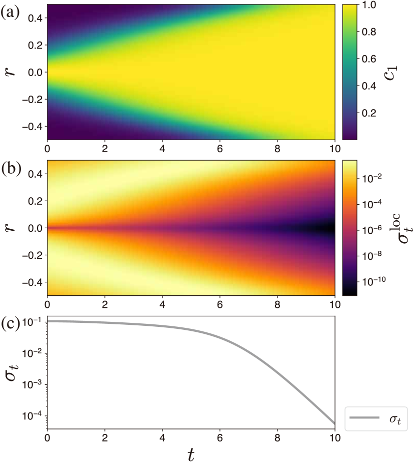
Figure 5: (a) The time series of $c_{1}$ in the Fisher–KPP equation. The area with high $c_{1}$ (yellow) expands as time passes. (b) The local EPR $\sigma^{\mathrm{loc}}_{t}$ in the Fisher–KPP equation. The local EPR is colored on a logarithmic scale. Comparing (a) with (b), we can see that dissipation occurs at the boundary between high- and low-concentration areas. (c) The EPR $\sigma_{t}$ in the Fisher–KPP equation. Reflecting the relaxation to the equilibrium state, the EPR is monotonically decreasing in time.

In Fig. 5, we numerically show the time series of the local EPR $\sigma_{t}^{\mathrm{loc}}(r)$ and the concentration distribution of the internal species $c_{1}$. As is well known, in the Fisher–KPP equation, the area of high concentration of $c_{1}$ spreads over time [77]: unlike normal diffusion, the total concentration is not conserved. The reaction does not occur inside the high-concentration area because $c_{1}=1$ is the equilibrium concentration of the reaction in Eq. (135) with given parameters. Diffusion also does not occur inside the high-concentration area because the concentration gradient disappears there. Thus, the local EPR is larger at the boundary between the high and low-concentration areas, and no dissipation occurs inside the high-concentration area.

Brusselator model.— The Brusselator model consists of two internal species, $Z_{1}$ and $Z_{2}$, an external species $Z_{3}$, and three reactions,

$$\ce{$Z_{3}$<=>C[$k^{+}_{1}$][$k^{-}_{1}$]$Z_{1}$},\quad\ce{$Z_{1}$<=>C[$k^{+}_{2}$][$k^{-}_{2}$]$Z_{2}$},\quad\ce{$2Z_{1}+Z_{2}$<=>C[$k^{+}_{3}$][$k^{-}_{3}$]$3Z_{1}$},$$ (139)

where we label the reactions $\rho=1$, $2$, $3$ from left to right. The index sets are $\mathcal{S}=\{1,2,3\}$, $\mathcal{X}=\{1,2\}$, $\mathcal{Y}=\{3\}$, $\mathcal{R}=\{1,2,3\}$, and $\mathcal{R}_{\mathcal{X}}=\{1,2,3\}=\mathcal{R}$, and the vectors $\mathchoice{\kern-0.15pt\overset{\kern 0.7pt\smash{\lower 1.07639pt\hbox{\scalebox{0.45}{$\bm{\rightarrow}$}}}\kern-0.3pt}{c}}{\kern-0.15pt\overset{\kern 0.7pt\smash{\lower 1.07639pt\hbox{\scalebox{0.45}{$\bm{\rightarrow}$}}}\kern-0.3pt}{c}}{\overset{\smash{\lower 0.6458pt\hbox{\kern 0.2pt\scalebox{0.3}{$\bm{\rightarrow}$}\kern-0.8pt}}}{c}}{\overset{\smash{\lower 0.6458pt\hbox{\kern 0.2pt\scalebox{0.3}{$\bm{\rightarrow}$}\kern-0.8pt}}}{c}}=(c_{1},c_{2},c_{3}){}^{\top}$, $\mathchoice{\kern-0.15pt\overset{\kern 0.7pt\smash{\lower 1.07639pt\hbox{\scalebox{0.45}{$\bm{\rightarrow}$}}}\kern-0.3pt}{c}}{\kern-0.15pt\overset{\kern 0.7pt\smash{\lower 1.07639pt\hbox{\scalebox{0.45}{$\bm{\rightarrow}$}}}\kern-0.3pt}{c}}{\overset{\smash{\lower 0.6458pt\hbox{\kern 0.2pt\scalebox{0.3}{$\bm{\rightarrow}$}\kern-0.8pt}}}{c}}{\overset{\smash{\lower 0.6458pt\hbox{\kern 0.2pt\scalebox{0.3}{$\bm{\rightarrow}$}\kern-0.8pt}}}{c}}_{\mathcal{X}}=(c_{1},c_{2}){}^{\top}$, and $\mathchoice{\kern-0.15pt\overset{\kern 0.7pt\smash{\lower 1.07639pt\hbox{\scalebox{0.45}{$\bm{\rightarrow}$}}}\kern-0.3pt}{c}}{\kern-0.15pt\overset{\kern 0.7pt\smash{\lower 1.07639pt\hbox{\scalebox{0.45}{$\bm{\rightarrow}$}}}\kern-0.3pt}{c}}{\overset{\smash{\lower 0.6458pt\hbox{\kern 0.2pt\scalebox{0.3}{$\bm{\rightarrow}$}\kern-0.8pt}}}{c}}{\overset{\smash{\lower 0.6458pt\hbox{\kern 0.2pt\scalebox{0.3}{$\bm{\rightarrow}$}\kern-0.8pt}}}{c}}_{\mathcal{Y}}=(c_{3})$. The stoichiometric matrix is

The concentration of the external species is again assumed to be homogeneous due to the interaction with the outside: $c_{3}(r;t)=1$ holds for all $r\in V_{1}$. We let the mobility tensor have the simple form in Eq. (60) and assume Fick’s law for the diffusion currents, $J_{(\alpha)}=-D_{\alpha}\partial_{r}c_{\alpha}$. Here, $J_{(3)}=0$ because $c_{3}$ is homogeneous and $\partial_{r}c_{3}=0$. We also assume the mass action kinetics for the reaction fluxes: $j^{+}_{1}(r;t)=k_{1}^{+}c_{3}(r;t)=k_{1}^{+}$, $j^{-}_{1}(r;t)=k_{1}^{-}c_{1}(r;t)$, $j^{+}_{2}(r;t)=k_{2}^{+}c_{1}(r;t)$, $j^{-}_{2}(r;t)=k_{2}^{-}c_{2}(r;t)$, $j^{+}_{3}(r;t)=k_{3}^{+}c_{1}(r;t)^{2}c_{2}(r;t)$, and $j^{-}_{1}(r;t)=k_{3}^{-}c_{1}(r;t)^{3}$. Then, the dynamics are given by

$$\partial_{t}c_{1}=D_{1}\partial_{r}^{2}c_{1}+k_{1}^{+}-k_{1}^{-}c_{1}$$

$$\phantom{\partial_{t}c_{1}=}-k_{2}^{+}c_{1}+k_{2}^{-}c_{2}+k_{3}^{+}c_{1}^{2}c_{2}-k_{3}^{-}c_{1}^{3}$$ (140)

$$\partial_{t}c_{2}=D_{2}\partial_{r}^{2}c_{2}+k_{2}^{+}c_{1}-k_{2}^{-}c_{2}-k_{3}^{+}c_{1}^{2}c_{2}+k_{3}^{-}c_{1}^{3}.$$ (141)

We impose the periodic boundary conditions. We set the parameters $D_{1}=1.6\times 10^{-4}$, $D_{2}=10^{-3}$, and $(k_{1}^{+},k_{1}^{-},k_{2}^{+},k_{2}^{-},k_{3}^{+},k_{3}^{-})=(1,1,10,0.1,1,1)$.

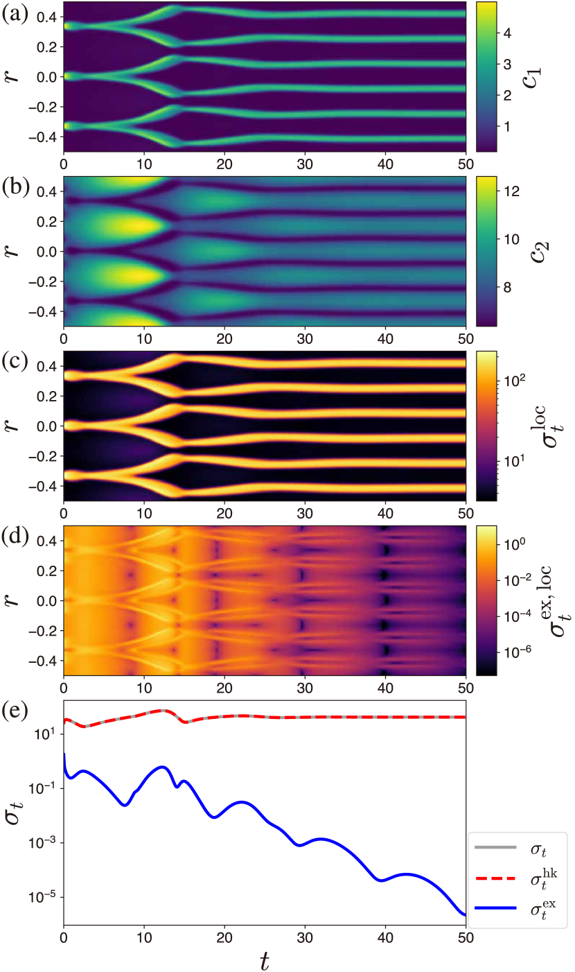
Figure 6: (a) The time series of $c_{1}$ in the Brusselator model. The symmetry of the pattern changes from $3$-fold symmetry to $6$-fold symmetry with time evolution. (b) The time series of $c_{2}$ in the Brusselator model. (c) The local EPR $\sigma^{\mathrm{loc}}_{t}$ in the Brusselator model. The local EPRs are colored on a logarithmic scale. In contrast to the Fisher–KPP equation [Fig 5(b)], $\sigma^{\mathrm{loc}}_{t}$ is large on the peaks of the pattern (areas where $c_{1}$ is high), not on the edges of the pattern. (d) The local excess EPR $\sigma^{\mathrm{ex,loc}}_{t}$ in the Brusselator model. At a given time, the value of $\sigma^{\mathrm{ex,loc}}_{t}$ at the peaks of the pattern is sufficiently greater than the values of $\sigma^{\mathrm{ex,loc}}$ at other positions. (e) The EPRs $\sigma_{t}$, $\sigma^{\mathrm{hk}}_{t}$, and $\sigma^{\mathrm{ex}}_{t}$ in the Brusselator model. The excess EPR $\sigma^{\mathrm{ex}}_{t}$ is considerably smaller than the others and approaches zero as the system approaches steady state. The EPR $\sigma_{t}$ does not vanish to maintain the pattern.

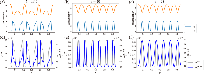
Figure 7: (a-c) The $r$-dependence of the concentrations $c_{1}$ and $c_{2}$ at $t=12.5$ [(a)], $t=40$ [(b)], and $t=48$ [(c)] in the Brusselator. (d-f) The $r$-dependence of the local EPRs $\sigma^{\rm loc}_{t}$ and $\sigma^{\rm loc,ex}_{t}$ at $t=12.5$ [(d)], $t=40$ [(e)], and $t=48$ [(f)] in the Brusselator. At $t=12.5$ and $t=40$ and $t=48$, the shapes of $\sigma^{\mathrm{loc}}_{t}$ [gray lines in (d-f)] are similar to the ones of $c_{1}$ [cyan lines in (a-c)]. The local excess EPR $\sigma^{\mathrm{ex,loc}}_{t}$ [blue lines in (d) and (e)] at $t=12.5$ and $t=40$ has peaks at the edges of the pattern. When the state is sufficiently close to the steady state ($t=48$), $\sigma^{\mathrm{ex,loc}}_{t}$ [blue lines in (f)] does not have peaks at the edges of the pattern.

For the Brusselator model, we can also explicitly write down the condition that determines the potential $\phi^{\ast}$ [Eq. (105)]. However, it is difficult to solve analytically, unlike the case of the Fisher–KPP equation, so we solve it numerically. In Fig. 6, we show the time series of $c_{1}$, $c_{2}$, $\sigma_{t}^{\mathrm{loc}}(r)$, $\sigma_{t}^{\mathrm{ex,loc}}(r)$, and the EPRs, numerically obtained. In contrast to the previous model, the local EPR $\sigma^{\mathrm{loc}}_{t}$ is large on the pattern (areas where $c_{1}$ is high), not on the edges of the pattern. On the other hand, the local excess EPR $\sigma^{\mathrm{ex,loc}}_{t}(r)$ is large on the edges of the pattern unless the system is close to the steady state. In Fig. 7, we compare their spatial profiles at three characteristic time points: one far from the steady state ($t=12.5$), one relatively close to the steady state ($t=40$), and one nearly at steady state ($t=48$). We can see that the excess EPR decreases (not monotonically) as the system approaches the steady state. In addition, the excess EPR $\sigma_{t}^{\mathrm{ex}}$ is much smaller than the EPR $\sigma_{t}$ as the majority of the dissipation is the housekeeping EPR, which is caused by cyclic currents not affecting the dynamics.

V Optimal transport and Thermodynamic speed limits for reaction-diffusion systems

We can understand dissipation in RDSs from the perspective of thermodynamic trade-off relations, which quantify the minimum dissipation required to achieve an objective. In particular, we focus on the thermodynamic speed limits (TSLs), which are trade-off relations between the speed of the dynamics and dissipation. They are geometric relations as they typically use some measure of “distance” between the initial and final patterns to quantify the speed. We measure the distance between two patterns of an RDS by the Wasserstein distance, similarly to Langevin systems and MJPs [33, 34, 36, 37, 38, 39, 40, 41, 42, 43, 44].

An RDS is a composite of chemical reactions and diffusive dynamics. Since some kinds of Wasserstein distance have been studied for both kinds of dynamics, we can generalize the $1$- and $2$-Wasserstein distances to RDSs to derive TSLs. Sections V.1 and V.2 are dedicated to the generalization, while some differences between these distances are discussed in Sec. V.3. We derive TSLs with the $1$- and $2$-Wasserstein distances for RDSs by utilizing a connection between the $2$-Wasserstein distance and the excess EPR in Sec. V.4. The final section V.5 provides numerical demonstrations of the $1$-Wasserstein distance and the TSLs.

We note that we need to specify boundary conditions to define the Wasserstein distance variationally (otherwise, it will not be well defined). We adopt here the boundary conditions discussed in Sec. III.2 for quantities that are considered as currents, e.g., a quantity obtained by acting the mobility tensor on a force.

V.1 1-Wasserstein distance for reaction-diffusion systems

We introduce the $1$-Wasserstein distance for the RDS as a distance between two concentration distributions of the internal species, as a generalization of the Benamou–Brenier formulation for Langevin systems in Eqs. (34) and (35), and that for MJPs [41].

We define it as

$${W}_{1,\mathcal{X}}\quantity(\mathchoice{\kern-0.15pt\overset{\kern 0.7pt\smash{\lower 1.07639pt\hbox{\scalebox{0.45}{$\bm{\rightarrow}$}}}\kern-0.3pt}{c}}{\kern-0.15pt\overset{\kern 0.7pt\smash{\lower 1.07639pt\hbox{\scalebox{0.45}{$\bm{\rightarrow}$}}}\kern-0.3pt}{c}}{\overset{\smash{\lower 0.6458pt\hbox{\kern 0.2pt\scalebox{0.3}{$\bm{\rightarrow}$}\kern-0.8pt}}}{c}}{\overset{\smash{\lower 0.6458pt\hbox{\kern 0.2pt\scalebox{0.3}{$\bm{\rightarrow}$}\kern-0.8pt}}}{c}}^{A},\mathchoice{\kern-0.15pt\overset{\kern 0.7pt\smash{\lower 1.07639pt\hbox{\scalebox{0.45}{$\bm{\rightarrow}$}}}\kern-0.3pt}{c}}{\kern-0.15pt\overset{\kern 0.7pt\smash{\lower 1.07639pt\hbox{\scalebox{0.45}{$\bm{\rightarrow}$}}}\kern-0.3pt}{c}}{\overset{\smash{\lower 0.6458pt\hbox{\kern 0.2pt\scalebox{0.3}{$\bm{\rightarrow}$}\kern-0.8pt}}}{c}}{\overset{\smash{\lower 0.6458pt\hbox{\kern 0.2pt\scalebox{0.3}{$\bm{\rightarrow}$}\kern-0.8pt}}}{c}}^{B})\coloneqq\inf_{\mathchoice{\kern-0.15pt\overset{\kern 0.7pt\smash{\lower 0.75346pt\hbox{\scalebox{0.45}{$\bm{\rightarrow}$}}}\kern-0.3pt}{c}}{\kern-0.15pt\overset{\kern 0.7pt\smash{\lower 0.75346pt\hbox{\scalebox{0.45}{$\bm{\rightarrow}$}}}\kern-0.3pt}{c}}{\overset{\smash{\lower 0.45206pt\hbox{\kern 0.2pt\scalebox{0.3}{$\bm{\rightarrow}$}\kern-0.8pt}}}{c}}{\overset{\smash{\lower 0.45206pt\hbox{\kern 0.2pt\scalebox{0.3}{$\bm{\rightarrow}$}\kern-0.8pt}}}{c}},\mathcal{J}^{\prime}}\quantity{\int^{\tau}_{0}dt\int_{V}d\bm{r}|\mathcal{J}^{\prime}|_{\rm RD}},$$ (142)

where

$$|\mathcal{J}^{\prime}|_{\rm RD}\coloneqq\sum_{\alpha\in\mathcal{S}}\|\bm{J}^{\prime}_{(\alpha)}\|+\sum_{\rho\in\mathcal{R}}|j^{\prime}_{\rho}|,$$ (143)

and $\mathchoice{\kern-0.15pt\overset{\kern 0.7pt\smash{\lower 1.07639pt\hbox{\scalebox{0.45}{$\bm{\rightarrow}$}}}\kern-0.3pt}{c}}{\kern-0.15pt\overset{\kern 0.7pt\smash{\lower 1.07639pt\hbox{\scalebox{0.45}{$\bm{\rightarrow}$}}}\kern-0.3pt}{c}}{\overset{\smash{\lower 0.6458pt\hbox{\kern 0.2pt\scalebox{0.3}{$\bm{\rightarrow}$}\kern-0.8pt}}}{c}}{\overset{\smash{\lower 0.6458pt\hbox{\kern 0.2pt\scalebox{0.3}{$\bm{\rightarrow}$}\kern-0.8pt}}}{c}}$ and $\mathcal{J}^{\prime}$ are such that

$$\partial_{t}\mathchoice{\kern-0.15pt\overset{\kern 0.7pt\smash{\lower 1.07639pt\hbox{\scalebox{0.45}{$\bm{\rightarrow}$}}}\kern-0.3pt}{c}}{\kern-0.15pt\overset{\kern 0.7pt\smash{\lower 1.07639pt\hbox{\scalebox{0.45}{$\bm{\rightarrow}$}}}\kern-0.3pt}{c}}{\overset{\smash{\lower 0.6458pt\hbox{\kern 0.2pt\scalebox{0.3}{$\bm{\rightarrow}$}\kern-0.8pt}}}{c}}{\overset{\smash{\lower 0.6458pt\hbox{\kern 0.2pt\scalebox{0.3}{$\bm{\rightarrow}$}\kern-0.8pt}}}{c}}_{\mathcal{X}}=\quantity(\nabla^{{\dagger}}\mathcal{J}^{\prime})_{\mathcal{X}},\;\mathchoice{\kern-0.15pt\overset{\kern 0.7pt\smash{\lower 1.07639pt\hbox{\scalebox{0.45}{$\bm{\rightarrow}$}}}\kern-0.3pt}{c}}{\kern-0.15pt\overset{\kern 0.7pt\smash{\lower 1.07639pt\hbox{\scalebox{0.45}{$\bm{\rightarrow}$}}}\kern-0.3pt}{c}}{\overset{\smash{\lower 0.6458pt\hbox{\kern 0.2pt\scalebox{0.3}{$\bm{\rightarrow}$}\kern-0.8pt}}}{c}}{\overset{\smash{\lower 0.6458pt\hbox{\kern 0.2pt\scalebox{0.3}{$\bm{\rightarrow}$}\kern-0.8pt}}}{c}}_{\mathcal{X}}(0)=\mathchoice{\kern-0.15pt\overset{\kern 0.7pt\smash{\lower 1.07639pt\hbox{\scalebox{0.45}{$\bm{\rightarrow}$}}}\kern-0.3pt}{c}}{\kern-0.15pt\overset{\kern 0.7pt\smash{\lower 1.07639pt\hbox{\scalebox{0.45}{$\bm{\rightarrow}$}}}\kern-0.3pt}{c}}{\overset{\smash{\lower 0.6458pt\hbox{\kern 0.2pt\scalebox{0.3}{$\bm{\rightarrow}$}\kern-0.8pt}}}{c}}{\overset{\smash{\lower 0.6458pt\hbox{\kern 0.2pt\scalebox{0.3}{$\bm{\rightarrow}$}\kern-0.8pt}}}{c}}^{A}_{\mathcal{X}},\mathchoice{\kern-0.15pt\overset{\kern 0.7pt\smash{\lower 1.07639pt\hbox{\scalebox{0.45}{$\bm{\rightarrow}$}}}\kern-0.3pt}{c}}{\kern-0.15pt\overset{\kern 0.7pt\smash{\lower 1.07639pt\hbox{\scalebox{0.45}{$\bm{\rightarrow}$}}}\kern-0.3pt}{c}}{\overset{\smash{\lower 0.6458pt\hbox{\kern 0.2pt\scalebox{0.3}{$\bm{\rightarrow}$}\kern-0.8pt}}}{c}}{\overset{\smash{\lower 0.6458pt\hbox{\kern 0.2pt\scalebox{0.3}{$\bm{\rightarrow}$}\kern-0.8pt}}}{c}}_{\mathcal{X}}(\tau)=\mathchoice{\kern-0.15pt\overset{\kern 0.7pt\smash{\lower 1.07639pt\hbox{\scalebox{0.45}{$\bm{\rightarrow}$}}}\kern-0.3pt}{c}}{\kern-0.15pt\overset{\kern 0.7pt\smash{\lower 1.07639pt\hbox{\scalebox{0.45}{$\bm{\rightarrow}$}}}\kern-0.3pt}{c}}{\overset{\smash{\lower 0.6458pt\hbox{\kern 0.2pt\scalebox{0.3}{$\bm{\rightarrow}$}\kern-0.8pt}}}{c}}{\overset{\smash{\lower 0.6458pt\hbox{\kern 0.2pt\scalebox{0.3}{$\bm{\rightarrow}$}\kern-0.8pt}}}{c}}^{B}_{\mathcal{X}}.$$ (144)

These constraints mean that the minimization is conducted over the time series that obeys the continuity equation with current $\mathcal{J}^{\prime}$ connecting $\mathchoice{\kern-0.15pt\overset{\kern 0.7pt\smash{\lower 1.07639pt\hbox{\scalebox{0.45}{$\bm{\rightarrow}$}}}\kern-0.3pt}{c}}{\kern-0.15pt\overset{\kern 0.7pt\smash{\lower 1.07639pt\hbox{\scalebox{0.45}{$\bm{\rightarrow}$}}}\kern-0.3pt}{c}}{\overset{\smash{\lower 0.6458pt\hbox{\kern 0.2pt\scalebox{0.3}{$\bm{\rightarrow}$}\kern-0.8pt}}}{c}}{\overset{\smash{\lower 0.6458pt\hbox{\kern 0.2pt\scalebox{0.3}{$\bm{\rightarrow}$}\kern-0.8pt}}}{c}}^{A}$ and $\mathchoice{\kern-0.15pt\overset{\kern 0.7pt\smash{\lower 1.07639pt\hbox{\scalebox{0.45}{$\bm{\rightarrow}$}}}\kern-0.3pt}{c}}{\kern-0.15pt\overset{\kern 0.7pt\smash{\lower 1.07639pt\hbox{\scalebox{0.45}{$\bm{\rightarrow}$}}}\kern-0.3pt}{c}}{\overset{\smash{\lower 0.6458pt\hbox{\kern 0.2pt\scalebox{0.3}{$\bm{\rightarrow}$}\kern-0.8pt}}}{c}}{\overset{\smash{\lower 0.6458pt\hbox{\kern 0.2pt\scalebox{0.3}{$\bm{\rightarrow}$}\kern-0.8pt}}}{c}}^{B}$ only with respect to the internal species.

Note that the concentrations of the external species are irrelevant in the formula. As a result, the $1$-Wasserstein distance can be zero even if $\mathchoice{\kern-0.15pt\overset{\kern 0.7pt\smash{\lower 1.07639pt\hbox{\scalebox{0.45}{$\bm{\rightarrow}$}}}\kern-0.3pt}{c}}{\kern-0.15pt\overset{\kern 0.7pt\smash{\lower 1.07639pt\hbox{\scalebox{0.45}{$\bm{\rightarrow}$}}}\kern-0.3pt}{c}}{\overset{\smash{\lower 0.6458pt\hbox{\kern 0.2pt\scalebox{0.3}{$\bm{\rightarrow}$}\kern-0.8pt}}}{c}}{\overset{\smash{\lower 0.6458pt\hbox{\kern 0.2pt\scalebox{0.3}{$\bm{\rightarrow}$}\kern-0.8pt}}}{c}}^{A}\neq\mathchoice{\kern-0.15pt\overset{\kern 0.7pt\smash{\lower 1.07639pt\hbox{\scalebox{0.45}{$\bm{\rightarrow}$}}}\kern-0.3pt}{c}}{\kern-0.15pt\overset{\kern 0.7pt\smash{\lower 1.07639pt\hbox{\scalebox{0.45}{$\bm{\rightarrow}$}}}\kern-0.3pt}{c}}{\overset{\smash{\lower 0.6458pt\hbox{\kern 0.2pt\scalebox{0.3}{$\bm{\rightarrow}$}\kern-0.8pt}}}{c}}{\overset{\smash{\lower 0.6458pt\hbox{\kern 0.2pt\scalebox{0.3}{$\bm{\rightarrow}$}\kern-0.8pt}}}{c}}^{B}$ as long as $\mathchoice{\kern-0.15pt\overset{\kern 0.7pt\smash{\lower 1.07639pt\hbox{\scalebox{0.45}{$\bm{\rightarrow}$}}}\kern-0.3pt}{c}}{\kern-0.15pt\overset{\kern 0.7pt\smash{\lower 1.07639pt\hbox{\scalebox{0.45}{$\bm{\rightarrow}$}}}\kern-0.3pt}{c}}{\overset{\smash{\lower 0.6458pt\hbox{\kern 0.2pt\scalebox{0.3}{$\bm{\rightarrow}$}\kern-0.8pt}}}{c}}{\overset{\smash{\lower 0.6458pt\hbox{\kern 0.2pt\scalebox{0.3}{$\bm{\rightarrow}$}\kern-0.8pt}}}{c}}^{A}_{\mathcal{X}}=\mathchoice{\kern-0.15pt\overset{\kern 0.7pt\smash{\lower 1.07639pt\hbox{\scalebox{0.45}{$\bm{\rightarrow}$}}}\kern-0.3pt}{c}}{\kern-0.15pt\overset{\kern 0.7pt\smash{\lower 1.07639pt\hbox{\scalebox{0.45}{$\bm{\rightarrow}$}}}\kern-0.3pt}{c}}{\overset{\smash{\lower 0.6458pt\hbox{\kern 0.2pt\scalebox{0.3}{$\bm{\rightarrow}$}\kern-0.8pt}}}{c}}{\overset{\smash{\lower 0.6458pt\hbox{\kern 0.2pt\scalebox{0.3}{$\bm{\rightarrow}$}\kern-0.8pt}}}{c}}^{B}_{\mathcal{X}}$. Therefore, it should be regarded as a distance between concentration distributions of internal species rather than whole concentration profiles.

We can also obtain the $1$-Wasserstein distance ${W}_{1,\mathcal{X}}$ by another optimization problem as

$${W}_{1,\mathcal{X}}\quantity(\mathchoice{\kern-0.15pt\overset{\kern 0.7pt\smash{\lower 1.07639pt\hbox{\scalebox{0.45}{$\bm{\rightarrow}$}}}\kern-0.3pt}{c}}{\kern-0.15pt\overset{\kern 0.7pt\smash{\lower 1.07639pt\hbox{\scalebox{0.45}{$\bm{\rightarrow}$}}}\kern-0.3pt}{c}}{\overset{\smash{\lower 0.6458pt\hbox{\kern 0.2pt\scalebox{0.3}{$\bm{\rightarrow}$}\kern-0.8pt}}}{c}}{\overset{\smash{\lower 0.6458pt\hbox{\kern 0.2pt\scalebox{0.3}{$\bm{\rightarrow}$}\kern-0.8pt}}}{c}}^{A},\mathchoice{\kern-0.15pt\overset{\kern 0.7pt\smash{\lower 1.07639pt\hbox{\scalebox{0.45}{$\bm{\rightarrow}$}}}\kern-0.3pt}{c}}{\kern-0.15pt\overset{\kern 0.7pt\smash{\lower 1.07639pt\hbox{\scalebox{0.45}{$\bm{\rightarrow}$}}}\kern-0.3pt}{c}}{\overset{\smash{\lower 0.6458pt\hbox{\kern 0.2pt\scalebox{0.3}{$\bm{\rightarrow}$}\kern-0.8pt}}}{c}}{\overset{\smash{\lower 0.6458pt\hbox{\kern 0.2pt\scalebox{0.3}{$\bm{\rightarrow}$}\kern-0.8pt}}}{c}}^{B})=\inf_{\mathcal{U}}\int_{V}d\bm{r}|\mathcal{U}|_{\rm RD},$$ (145)

with the condition

$$\mathchoice{\kern-0.15pt\overset{\kern 0.7pt\smash{\lower 1.07639pt\hbox{\scalebox{0.45}{$\bm{\rightarrow}$}}}\kern-0.3pt}{c}}{\kern-0.15pt\overset{\kern 0.7pt\smash{\lower 1.07639pt\hbox{\scalebox{0.45}{$\bm{\rightarrow}$}}}\kern-0.3pt}{c}}{\overset{\smash{\lower 0.6458pt\hbox{\kern 0.2pt\scalebox{0.3}{$\bm{\rightarrow}$}\kern-0.8pt}}}{c}}{\overset{\smash{\lower 0.6458pt\hbox{\kern 0.2pt\scalebox{0.3}{$\bm{\rightarrow}$}\kern-0.8pt}}}{c}}^{B}_{\mathcal{X}}-\mathchoice{\kern-0.15pt\overset{\kern 0.7pt\smash{\lower 1.07639pt\hbox{\scalebox{0.45}{$\bm{\rightarrow}$}}}\kern-0.3pt}{c}}{\kern-0.15pt\overset{\kern 0.7pt\smash{\lower 1.07639pt\hbox{\scalebox{0.45}{$\bm{\rightarrow}$}}}\kern-0.3pt}{c}}{\overset{\smash{\lower 0.6458pt\hbox{\kern 0.2pt\scalebox{0.3}{$\bm{\rightarrow}$}\kern-0.8pt}}}{c}}{\overset{\smash{\lower 0.6458pt\hbox{\kern 0.2pt\scalebox{0.3}{$\bm{\rightarrow}$}\kern-0.8pt}}}{c}}^{A}_{\mathcal{X}}=\quantity(\nabla^{{\dagger}}\mathcal{U})_{\mathcal{X}},$$ (146)

and the boundary condition on the diffusion part of $\mathcal{U}$ for the internal species. Using this optimization problem, we can compute ${W}_{1,\mathcal{X}}$ numerically with less computational complexity. We provide the derivation of Eq. (145) in Appendix E.1.

We can generalize the Kantorovich–Rubinstein duality [Eq. (36)] to RDSs (see the details in Appendix E.2). We only prove that the generalization of the Kantorovich–Rubinstein duality gives the lower bound of ${W}_{1,\mathcal{X}}$ defined in Eq. (142). This lower bound is regarded as weak duality [78, 79]. For any $d$-dimensional area $V$, it is not known whether the expression of Eq. (145) and the expression by the Kantorovich–Rubinstein duality coincide, namely, whether the strong duality holds [78, 79]. It is different from the case of Langevin systems on $V=\mathbb{R}^{d}$, where the strong duality holds.

V.2 2-Wasserstein distance for reaction-diffusion systems

We define the $2$-Wasserstein distance between concentration distributions of the internal species by fixing the concentration distribution of the external species as

$${W}_{2,\mathcal{X}}\quantity(\mathchoice{\kern-0.15pt\overset{\kern 0.7pt\smash{\lower 1.07639pt\hbox{\scalebox{0.45}{$\bm{\rightarrow}$}}}\kern-0.3pt}{c}}{\kern-0.15pt\overset{\kern 0.7pt\smash{\lower 1.07639pt\hbox{\scalebox{0.45}{$\bm{\rightarrow}$}}}\kern-0.3pt}{c}}{\overset{\smash{\lower 0.6458pt\hbox{\kern 0.2pt\scalebox{0.3}{$\bm{\rightarrow}$}\kern-0.8pt}}}{c}}{\overset{\smash{\lower 0.6458pt\hbox{\kern 0.2pt\scalebox{0.3}{$\bm{\rightarrow}$}\kern-0.8pt}}}{c}}^{A},\mathchoice{\kern-0.15pt\overset{\kern 0.7pt\smash{\lower 1.07639pt\hbox{\scalebox{0.45}{$\bm{\rightarrow}$}}}\kern-0.3pt}{c}}{\kern-0.15pt\overset{\kern 0.7pt\smash{\lower 1.07639pt\hbox{\scalebox{0.45}{$\bm{\rightarrow}$}}}\kern-0.3pt}{c}}{\overset{\smash{\lower 0.6458pt\hbox{\kern 0.2pt\scalebox{0.3}{$\bm{\rightarrow}$}\kern-0.8pt}}}{c}}{\overset{\smash{\lower 0.6458pt\hbox{\kern 0.2pt\scalebox{0.3}{$\bm{\rightarrow}$}\kern-0.8pt}}}{c}}^{B}\middle|\mathchoice{\kern-0.15pt\overset{\kern 0.7pt\smash{\lower 1.07639pt\hbox{\scalebox{0.45}{$\bm{\rightarrow}$}}}\kern-0.3pt}{b}}{\kern-0.15pt\overset{\kern 0.7pt\smash{\lower 1.07639pt\hbox{\scalebox{0.45}{$\bm{\rightarrow}$}}}\kern-0.3pt}{b}}{\overset{\smash{\lower 0.6458pt\hbox{\kern 0.2pt\scalebox{0.3}{$\bm{\rightarrow}$}\kern-0.8pt}}}{b}}{\overset{\smash{\lower 0.6458pt\hbox{\kern 0.2pt\scalebox{0.3}{$\bm{\rightarrow}$}\kern-0.8pt}}}{b}}_{\mathcal{Y}})^{2}\coloneqq\inf_{\mathchoice{\kern-0.15pt\overset{\kern 0.7pt\smash{\lower 0.75346pt\hbox{\scalebox{0.45}{$\bm{\rightarrow}$}}}\kern-0.3pt}{c}}{\kern-0.15pt\overset{\kern 0.7pt\smash{\lower 0.75346pt\hbox{\scalebox{0.45}{$\bm{\rightarrow}$}}}\kern-0.3pt}{c}}{\overset{\smash{\lower 0.45206pt\hbox{\kern 0.2pt\scalebox{0.3}{$\bm{\rightarrow}$}\kern-0.8pt}}}{c}}{\overset{\smash{\lower 0.45206pt\hbox{\kern 0.2pt\scalebox{0.3}{$\bm{\rightarrow}$}\kern-0.8pt}}}{c}},\mathcal{F}^{\prime}}\quantity{\tau\int^{\tau}_{0}\mathrm{d}t\left\llangle\mathcal{F}^{\prime},\mathcal{F}^{\prime}\right\rrangle_{\mathcal{M}_{\mathchoice{\kern-0.15pt\overset{\kern 0.7pt\smash{\lower 0.5382pt\hbox{\scalebox{0.45}{$\bm{\rightarrow}$}}}\kern-0.3pt}{c}}{\kern-0.15pt\overset{\kern 0.7pt\smash{\lower 0.5382pt\hbox{\scalebox{0.45}{$\bm{\rightarrow}$}}}\kern-0.3pt}{c}}{\overset{\smash{\lower 0.32289pt\hbox{\kern 0.2pt\scalebox{0.3}{$\bm{\rightarrow}$}\kern-0.8pt}}}{c}}{\overset{\smash{\lower 0.32289pt\hbox{\kern 0.2pt\scalebox{0.3}{$\bm{\rightarrow}$}\kern-0.8pt}}}{c}}}}},$$ (147)

where we impose the conditions

$$\partial_{t}\mathchoice{\kern-0.15pt\overset{\kern 0.7pt\smash{\lower 1.07639pt\hbox{\scalebox{0.45}{$\bm{\rightarrow}$}}}\kern-0.3pt}{c}}{\kern-0.15pt\overset{\kern 0.7pt\smash{\lower 1.07639pt\hbox{\scalebox{0.45}{$\bm{\rightarrow}$}}}\kern-0.3pt}{c}}{\overset{\smash{\lower 0.6458pt\hbox{\kern 0.2pt\scalebox{0.3}{$\bm{\rightarrow}$}\kern-0.8pt}}}{c}}{\overset{\smash{\lower 0.6458pt\hbox{\kern 0.2pt\scalebox{0.3}{$\bm{\rightarrow}$}\kern-0.8pt}}}{c}}_{\mathcal{X}}=\quantity(\nabla^{{\dagger}}\mathcal{M}_{\mathchoice{\kern-0.15pt\overset{\kern 0.7pt\smash{\lower 0.75346pt\hbox{\scalebox{0.45}{$\bm{\rightarrow}$}}}\kern-0.3pt}{c}}{\kern-0.15pt\overset{\kern 0.7pt\smash{\lower 0.75346pt\hbox{\scalebox{0.45}{$\bm{\rightarrow}$}}}\kern-0.3pt}{c}}{\overset{\smash{\lower 0.45206pt\hbox{\kern 0.2pt\scalebox{0.3}{$\bm{\rightarrow}$}\kern-0.8pt}}}{c}}{\overset{\smash{\lower 0.45206pt\hbox{\kern 0.2pt\scalebox{0.3}{$\bm{\rightarrow}$}\kern-0.8pt}}}{c}}}\mathcal{F}^{\prime})_{\mathcal{X}},$$ (148)

$$\mathchoice{\kern-0.15pt\overset{\kern 0.7pt\smash{\lower 1.07639pt\hbox{\scalebox{0.45}{$\bm{\rightarrow}$}}}\kern-0.3pt}{c}}{\kern-0.15pt\overset{\kern 0.7pt\smash{\lower 1.07639pt\hbox{\scalebox{0.45}{$\bm{\rightarrow}$}}}\kern-0.3pt}{c}}{\overset{\smash{\lower 0.6458pt\hbox{\kern 0.2pt\scalebox{0.3}{$\bm{\rightarrow}$}\kern-0.8pt}}}{c}}{\overset{\smash{\lower 0.6458pt\hbox{\kern 0.2pt\scalebox{0.3}{$\bm{\rightarrow}$}\kern-0.8pt}}}{c}}_{\mathcal{X}}(0)=\mathchoice{\kern-0.15pt\overset{\kern 0.7pt\smash{\lower 1.07639pt\hbox{\scalebox{0.45}{$\bm{\rightarrow}$}}}\kern-0.3pt}{c}}{\kern-0.15pt\overset{\kern 0.7pt\smash{\lower 1.07639pt\hbox{\scalebox{0.45}{$\bm{\rightarrow}$}}}\kern-0.3pt}{c}}{\overset{\smash{\lower 0.6458pt\hbox{\kern 0.2pt\scalebox{0.3}{$\bm{\rightarrow}$}\kern-0.8pt}}}{c}}{\overset{\smash{\lower 0.6458pt\hbox{\kern 0.2pt\scalebox{0.3}{$\bm{\rightarrow}$}\kern-0.8pt}}}{c}}^{A}_{\mathcal{X}},\;\mathchoice{\kern-0.15pt\overset{\kern 0.7pt\smash{\lower 1.07639pt\hbox{\scalebox{0.45}{$\bm{\rightarrow}$}}}\kern-0.3pt}{c}}{\kern-0.15pt\overset{\kern 0.7pt\smash{\lower 1.07639pt\hbox{\scalebox{0.45}{$\bm{\rightarrow}$}}}\kern-0.3pt}{c}}{\overset{\smash{\lower 0.6458pt\hbox{\kern 0.2pt\scalebox{0.3}{$\bm{\rightarrow}$}\kern-0.8pt}}}{c}}{\overset{\smash{\lower 0.6458pt\hbox{\kern 0.2pt\scalebox{0.3}{$\bm{\rightarrow}$}\kern-0.8pt}}}{c}}_{\mathcal{X}}(\tau)=\mathchoice{\kern-0.15pt\overset{\kern 0.7pt\smash{\lower 1.07639pt\hbox{\scalebox{0.45}{$\bm{\rightarrow}$}}}\kern-0.3pt}{c}}{\kern-0.15pt\overset{\kern 0.7pt\smash{\lower 1.07639pt\hbox{\scalebox{0.45}{$\bm{\rightarrow}$}}}\kern-0.3pt}{c}}{\overset{\smash{\lower 0.6458pt\hbox{\kern 0.2pt\scalebox{0.3}{$\bm{\rightarrow}$}\kern-0.8pt}}}{c}}{\overset{\smash{\lower 0.6458pt\hbox{\kern 0.2pt\scalebox{0.3}{$\bm{\rightarrow}$}\kern-0.8pt}}}{c}}^{B}_{\mathcal{X}},$$ (149)

and

$$\mathchoice{\kern-0.15pt\overset{\kern 0.7pt\smash{\lower 1.07639pt\hbox{\scalebox{0.45}{$\bm{\rightarrow}$}}}\kern-0.3pt}{c}}{\kern-0.15pt\overset{\kern 0.7pt\smash{\lower 1.07639pt\hbox{\scalebox{0.45}{$\bm{\rightarrow}$}}}\kern-0.3pt}{c}}{\overset{\smash{\lower 0.6458pt\hbox{\kern 0.2pt\scalebox{0.3}{$\bm{\rightarrow}$}\kern-0.8pt}}}{c}}{\overset{\smash{\lower 0.6458pt\hbox{\kern 0.2pt\scalebox{0.3}{$\bm{\rightarrow}$}\kern-0.8pt}}}{c}}^{A}_{\mathcal{Y}}=\mathchoice{\kern-0.15pt\overset{\kern 0.7pt\smash{\lower 1.07639pt\hbox{\scalebox{0.45}{$\bm{\rightarrow}$}}}\kern-0.3pt}{c}}{\kern-0.15pt\overset{\kern 0.7pt\smash{\lower 1.07639pt\hbox{\scalebox{0.45}{$\bm{\rightarrow}$}}}\kern-0.3pt}{c}}{\overset{\smash{\lower 0.6458pt\hbox{\kern 0.2pt\scalebox{0.3}{$\bm{\rightarrow}$}\kern-0.8pt}}}{c}}{\overset{\smash{\lower 0.6458pt\hbox{\kern 0.2pt\scalebox{0.3}{$\bm{\rightarrow}$}\kern-0.8pt}}}{c}}^{B}_{\mathcal{Y}}=\mathchoice{\kern-0.15pt\overset{\kern 0.7pt\smash{\lower 1.07639pt\hbox{\scalebox{0.45}{$\bm{\rightarrow}$}}}\kern-0.3pt}{c}}{\kern-0.15pt\overset{\kern 0.7pt\smash{\lower 1.07639pt\hbox{\scalebox{0.45}{$\bm{\rightarrow}$}}}\kern-0.3pt}{c}}{\overset{\smash{\lower 0.6458pt\hbox{\kern 0.2pt\scalebox{0.3}{$\bm{\rightarrow}$}\kern-0.8pt}}}{c}}{\overset{\smash{\lower 0.6458pt\hbox{\kern 0.2pt\scalebox{0.3}{$\bm{\rightarrow}$}\kern-0.8pt}}}{c}}_{\mathcal{Y}}(t)=\mathchoice{\kern-0.15pt\overset{\kern 0.7pt\smash{\lower 1.07639pt\hbox{\scalebox{0.45}{$\bm{\rightarrow}$}}}\kern-0.3pt}{b}}{\kern-0.15pt\overset{\kern 0.7pt\smash{\lower 1.07639pt\hbox{\scalebox{0.45}{$\bm{\rightarrow}$}}}\kern-0.3pt}{b}}{\overset{\smash{\lower 0.6458pt\hbox{\kern 0.2pt\scalebox{0.3}{$\bm{\rightarrow}$}\kern-0.8pt}}}{b}}{\overset{\smash{\lower 0.6458pt\hbox{\kern 0.2pt\scalebox{0.3}{$\bm{\rightarrow}$}\kern-0.8pt}}}{b}}_{\mathcal{Y}},$$ (150)

on $\mathchoice{\kern-0.15pt\overset{\kern 0.7pt\smash{\lower 1.07639pt\hbox{\scalebox{0.45}{$\bm{\rightarrow}$}}}\kern-0.3pt}{c}}{\kern-0.15pt\overset{\kern 0.7pt\smash{\lower 1.07639pt\hbox{\scalebox{0.45}{$\bm{\rightarrow}$}}}\kern-0.3pt}{c}}{\overset{\smash{\lower 0.6458pt\hbox{\kern 0.2pt\scalebox{0.3}{$\bm{\rightarrow}$}\kern-0.8pt}}}{c}}{\overset{\smash{\lower 0.6458pt\hbox{\kern 0.2pt\scalebox{0.3}{$\bm{\rightarrow}$}\kern-0.8pt}}}{c}}$ and $\mathcal{F}^{\prime}$ with time-independent concentration distribution $\mathchoice{\kern-0.15pt\overset{\kern 0.7pt\smash{\lower 1.07639pt\hbox{\scalebox{0.45}{$\bm{\rightarrow}$}}}\kern-0.3pt}{b}}{\kern-0.15pt\overset{\kern 0.7pt\smash{\lower 1.07639pt\hbox{\scalebox{0.45}{$\bm{\rightarrow}$}}}\kern-0.3pt}{b}}{\overset{\smash{\lower 0.6458pt\hbox{\kern 0.2pt\scalebox{0.3}{$\bm{\rightarrow}$}\kern-0.8pt}}}{b}}{\overset{\smash{\lower 0.6458pt\hbox{\kern 0.2pt\scalebox{0.3}{$\bm{\rightarrow}$}\kern-0.8pt}}}{b}}$. In particular, the conditions in Eq. (150) correspond to the concentration of the external species being fixed. Here, we write $\mathcal{M}_{\mathchoice{\kern-0.15pt\overset{\kern 0.7pt\smash{\lower 0.75346pt\hbox{\scalebox{0.45}{$\bm{\rightarrow}$}}}\kern-0.3pt}{c}}{\kern-0.15pt\overset{\kern 0.7pt\smash{\lower 0.75346pt\hbox{\scalebox{0.45}{$\bm{\rightarrow}$}}}\kern-0.3pt}{c}}{\overset{\smash{\lower 0.45206pt\hbox{\kern 0.2pt\scalebox{0.3}{$\bm{\rightarrow}$}\kern-0.8pt}}}{c}}{\overset{\smash{\lower 0.45206pt\hbox{\kern 0.2pt\scalebox{0.3}{$\bm{\rightarrow}$}\kern-0.8pt}}}{c}}}$ instead of $\mathcal{M}$ because we want to emphasize its dependence on concentration $\mathchoice{\kern-0.15pt\overset{\kern 0.7pt\smash{\lower 1.07639pt\hbox{\scalebox{0.45}{$\bm{\rightarrow}$}}}\kern-0.3pt}{c}}{\kern-0.15pt\overset{\kern 0.7pt\smash{\lower 1.07639pt\hbox{\scalebox{0.45}{$\bm{\rightarrow}$}}}\kern-0.3pt}{c}}{\overset{\smash{\lower 0.6458pt\hbox{\kern 0.2pt\scalebox{0.3}{$\bm{\rightarrow}$}\kern-0.8pt}}}{c}}{\overset{\smash{\lower 0.6458pt\hbox{\kern 0.2pt\scalebox{0.3}{$\bm{\rightarrow}$}\kern-0.8pt}}}{c}}$. In addition, we assume that $\overset{\smash{\lower 1.07639pt\hbox{\scalebox{0.7}[0.45]{$\bm{\leftrightarrow}$}}}}{\mathsf{M}}$ and $\mathsf{m}$ depend on time only through $\mathchoice{\kern-0.15pt\overset{\kern 0.7pt\smash{\lower 1.07639pt\hbox{\scalebox{0.45}{$\bm{\rightarrow}$}}}\kern-0.3pt}{c}}{\kern-0.15pt\overset{\kern 0.7pt\smash{\lower 1.07639pt\hbox{\scalebox{0.45}{$\bm{\rightarrow}$}}}\kern-0.3pt}{c}}{\overset{\smash{\lower 0.6458pt\hbox{\kern 0.2pt\scalebox{0.3}{$\bm{\rightarrow}$}\kern-0.8pt}}}{c}}{\overset{\smash{\lower 0.6458pt\hbox{\kern 0.2pt\scalebox{0.3}{$\bm{\rightarrow}$}\kern-0.8pt}}}{c}}$ and not explicitly, so that let ${W}_{2,\mathcal{X}}$ is invariant to changes of the parameter $\tau$.

This definition generalizes the Benamou–Brenier formula of the $2$-Wasserstein distance for Langevin systems in Eq. (32), MJPs [80], and CRNs [40]. This $2$-Wasserstein distance is also defined as the dissipation distance [59, 60] in the context of the gradient flow structure of RDSs.

The $2$-Wasserstein distance ${W}_{2,\mathcal{X}}(\mathchoice{\kern-0.15pt\overset{\kern 0.7pt\smash{\lower 1.07639pt\hbox{\scalebox{0.45}{$\bm{\rightarrow}$}}}\kern-0.3pt}{c}}{\kern-0.15pt\overset{\kern 0.7pt\smash{\lower 1.07639pt\hbox{\scalebox{0.45}{$\bm{\rightarrow}$}}}\kern-0.3pt}{c}}{\overset{\smash{\lower 0.6458pt\hbox{\kern 0.2pt\scalebox{0.3}{$\bm{\rightarrow}$}\kern-0.8pt}}}{c}}{\overset{\smash{\lower 0.6458pt\hbox{\kern 0.2pt\scalebox{0.3}{$\bm{\rightarrow}$}\kern-0.8pt}}}{c}}^{A},\mathchoice{\kern-0.15pt\overset{\kern 0.7pt\smash{\lower 1.07639pt\hbox{\scalebox{0.45}{$\bm{\rightarrow}$}}}\kern-0.3pt}{c}}{\kern-0.15pt\overset{\kern 0.7pt\smash{\lower 1.07639pt\hbox{\scalebox{0.45}{$\bm{\rightarrow}$}}}\kern-0.3pt}{c}}{\overset{\smash{\lower 0.6458pt\hbox{\kern 0.2pt\scalebox{0.3}{$\bm{\rightarrow}$}\kern-0.8pt}}}{c}}{\overset{\smash{\lower 0.6458pt\hbox{\kern 0.2pt\scalebox{0.3}{$\bm{\rightarrow}$}\kern-0.8pt}}}{c}}^{B}|\mathchoice{\kern-0.15pt\overset{\kern 0.7pt\smash{\lower 1.07639pt\hbox{\scalebox{0.45}{$\bm{\rightarrow}$}}}\kern-0.3pt}{b}}{\kern-0.15pt\overset{\kern 0.7pt\smash{\lower 1.07639pt\hbox{\scalebox{0.45}{$\bm{\rightarrow}$}}}\kern-0.3pt}{b}}{\overset{\smash{\lower 0.6458pt\hbox{\kern 0.2pt\scalebox{0.3}{$\bm{\rightarrow}$}\kern-0.8pt}}}{b}}{\overset{\smash{\lower 0.6458pt\hbox{\kern 0.2pt\scalebox{0.3}{$\bm{\rightarrow}$}\kern-0.8pt}}}{b}}_{\mathcal{Y}})$ is not a distance between concentration distributions of all species, but only those of the internal species, same as the $1$-Wasserstein distance ${W}_{1,\mathcal{X}}(\mathchoice{\kern-0.15pt\overset{\kern 0.7pt\smash{\lower 1.07639pt\hbox{\scalebox{0.45}{$\bm{\rightarrow}$}}}\kern-0.3pt}{c}}{\kern-0.15pt\overset{\kern 0.7pt\smash{\lower 1.07639pt\hbox{\scalebox{0.45}{$\bm{\rightarrow}$}}}\kern-0.3pt}{c}}{\overset{\smash{\lower 0.6458pt\hbox{\kern 0.2pt\scalebox{0.3}{$\bm{\rightarrow}$}\kern-0.8pt}}}{c}}{\overset{\smash{\lower 0.6458pt\hbox{\kern 0.2pt\scalebox{0.3}{$\bm{\rightarrow}$}\kern-0.8pt}}}{c}}^{A},\mathchoice{\kern-0.15pt\overset{\kern 0.7pt\smash{\lower 1.07639pt\hbox{\scalebox{0.45}{$\bm{\rightarrow}$}}}\kern-0.3pt}{c}}{\kern-0.15pt\overset{\kern 0.7pt\smash{\lower 1.07639pt\hbox{\scalebox{0.45}{$\bm{\rightarrow}$}}}\kern-0.3pt}{c}}{\overset{\smash{\lower 0.6458pt\hbox{\kern 0.2pt\scalebox{0.3}{$\bm{\rightarrow}$}\kern-0.8pt}}}{c}}{\overset{\smash{\lower 0.6458pt\hbox{\kern 0.2pt\scalebox{0.3}{$\bm{\rightarrow}$}\kern-0.8pt}}}{c}}^{B})$. This is because we fix the concentration distribution of the external species $\mathchoice{\kern-0.15pt\overset{\kern 0.7pt\smash{\lower 1.07639pt\hbox{\scalebox{0.45}{$\bm{\rightarrow}$}}}\kern-0.3pt}{c}}{\kern-0.15pt\overset{\kern 0.7pt\smash{\lower 1.07639pt\hbox{\scalebox{0.45}{$\bm{\rightarrow}$}}}\kern-0.3pt}{c}}{\overset{\smash{\lower 0.6458pt\hbox{\kern 0.2pt\scalebox{0.3}{$\bm{\rightarrow}$}\kern-0.8pt}}}{c}}{\overset{\smash{\lower 0.6458pt\hbox{\kern 0.2pt\scalebox{0.3}{$\bm{\rightarrow}$}\kern-0.8pt}}}{c}}_{\mathcal{Y}}(t)$ to $\mathchoice{\kern-0.15pt\overset{\kern 0.7pt\smash{\lower 1.07639pt\hbox{\scalebox{0.45}{$\bm{\rightarrow}$}}}\kern-0.3pt}{b}}{\kern-0.15pt\overset{\kern 0.7pt\smash{\lower 1.07639pt\hbox{\scalebox{0.45}{$\bm{\rightarrow}$}}}\kern-0.3pt}{b}}{\overset{\smash{\lower 0.6458pt\hbox{\kern 0.2pt\scalebox{0.3}{$\bm{\rightarrow}$}\kern-0.8pt}}}{b}}{\overset{\smash{\lower 0.6458pt\hbox{\kern 0.2pt\scalebox{0.3}{$\bm{\rightarrow}$}\kern-0.8pt}}}{b}}_{\mathcal{Y}}$ in the condition [Eq. (150)].

We can rewrite Eq. (147) in the form of an optimization problem not for the force $\mathcal{F}^{\prime}$ but for the potential $\mathchoice{\kern-0.15pt\overset{\kern 0.7pt\smash{\lower 1.07639pt\hbox{\scalebox{0.45}{$\bm{\rightarrow}$}}}\kern-0.3pt}{\phi}}{\kern-0.15pt\overset{\kern 0.7pt\smash{\lower 1.07639pt\hbox{\scalebox{0.45}{$\bm{\rightarrow}$}}}\kern-0.3pt}{\phi}}{\overset{\smash{\lower 0.6458pt\hbox{\kern 0.2pt\scalebox{0.3}{$\bm{\rightarrow}$}\kern-0.8pt}}}{\phi}}{\overset{\smash{\lower 0.6458pt\hbox{\kern 0.2pt\scalebox{0.3}{$\bm{\rightarrow}$}\kern-0.8pt}}}{\phi}}$ as

$${W}_{2,\mathcal{X}}\quantity(\mathchoice{\kern-0.15pt\overset{\kern 0.7pt\smash{\lower 1.07639pt\hbox{\scalebox{0.45}{$\bm{\rightarrow}$}}}\kern-0.3pt}{c}}{\kern-0.15pt\overset{\kern 0.7pt\smash{\lower 1.07639pt\hbox{\scalebox{0.45}{$\bm{\rightarrow}$}}}\kern-0.3pt}{c}}{\overset{\smash{\lower 0.6458pt\hbox{\kern 0.2pt\scalebox{0.3}{$\bm{\rightarrow}$}\kern-0.8pt}}}{c}}{\overset{\smash{\lower 0.6458pt\hbox{\kern 0.2pt\scalebox{0.3}{$\bm{\rightarrow}$}\kern-0.8pt}}}{c}}^{A},\mathchoice{\kern-0.15pt\overset{\kern 0.7pt\smash{\lower 1.07639pt\hbox{\scalebox{0.45}{$\bm{\rightarrow}$}}}\kern-0.3pt}{c}}{\kern-0.15pt\overset{\kern 0.7pt\smash{\lower 1.07639pt\hbox{\scalebox{0.45}{$\bm{\rightarrow}$}}}\kern-0.3pt}{c}}{\overset{\smash{\lower 0.6458pt\hbox{\kern 0.2pt\scalebox{0.3}{$\bm{\rightarrow}$}\kern-0.8pt}}}{c}}{\overset{\smash{\lower 0.6458pt\hbox{\kern 0.2pt\scalebox{0.3}{$\bm{\rightarrow}$}\kern-0.8pt}}}{c}}^{B}\middle|\mathchoice{\kern-0.15pt\overset{\kern 0.7pt\smash{\lower 1.07639pt\hbox{\scalebox{0.45}{$\bm{\rightarrow}$}}}\kern-0.3pt}{b}}{\kern-0.15pt\overset{\kern 0.7pt\smash{\lower 1.07639pt\hbox{\scalebox{0.45}{$\bm{\rightarrow}$}}}\kern-0.3pt}{b}}{\overset{\smash{\lower 0.6458pt\hbox{\kern 0.2pt\scalebox{0.3}{$\bm{\rightarrow}$}\kern-0.8pt}}}{b}}{\overset{\smash{\lower 0.6458pt\hbox{\kern 0.2pt\scalebox{0.3}{$\bm{\rightarrow}$}\kern-0.8pt}}}{b}}_{\mathcal{Y}})^{2}\coloneqq\inf_{\mathchoice{\kern-0.15pt\overset{\kern 0.7pt\smash{\lower 0.75346pt\hbox{\scalebox{0.45}{$\bm{\rightarrow}$}}}\kern-0.3pt}{\phi}}{\kern-0.15pt\overset{\kern 0.7pt\smash{\lower 0.75346pt\hbox{\scalebox{0.45}{$\bm{\rightarrow}$}}}\kern-0.3pt}{\phi}}{\overset{\smash{\lower 0.45206pt\hbox{\kern 0.2pt\scalebox{0.3}{$\bm{\rightarrow}$}\kern-0.8pt}}}{\phi}}{\overset{\smash{\lower 0.45206pt\hbox{\kern 0.2pt\scalebox{0.3}{$\bm{\rightarrow}$}\kern-0.8pt}}}{\phi}},\mathchoice{\kern-0.15pt\overset{\kern 0.7pt\smash{\lower 0.75346pt\hbox{\scalebox{0.45}{$\bm{\rightarrow}$}}}\kern-0.3pt}{c}}{\kern-0.15pt\overset{\kern 0.7pt\smash{\lower 0.75346pt\hbox{\scalebox{0.45}{$\bm{\rightarrow}$}}}\kern-0.3pt}{c}}{\overset{\smash{\lower 0.45206pt\hbox{\kern 0.2pt\scalebox{0.3}{$\bm{\rightarrow}$}\kern-0.8pt}}}{c}}{\overset{\smash{\lower 0.45206pt\hbox{\kern 0.2pt\scalebox{0.3}{$\bm{\rightarrow}$}\kern-0.8pt}}}{c}}}\quantity{\tau\int^{\tau}_{0}\mathrm{d}t\left\llangle\nabla\mathchoice{\kern-0.15pt\overset{\kern 0.7pt\smash{\lower 1.07639pt\hbox{\scalebox{0.45}{$\bm{\rightarrow}$}}}\kern-0.3pt}{\phi}}{\kern-0.15pt\overset{\kern 0.7pt\smash{\lower 1.07639pt\hbox{\scalebox{0.45}{$\bm{\rightarrow}$}}}\kern-0.3pt}{\phi}}{\overset{\smash{\lower 0.6458pt\hbox{\kern 0.2pt\scalebox{0.3}{$\bm{\rightarrow}$}\kern-0.8pt}}}{\phi}}{\overset{\smash{\lower 0.6458pt\hbox{\kern 0.2pt\scalebox{0.3}{$\bm{\rightarrow}$}\kern-0.8pt}}}{\phi}},\nabla\mathchoice{\kern-0.15pt\overset{\kern 0.7pt\smash{\lower 1.07639pt\hbox{\scalebox{0.45}{$\bm{\rightarrow}$}}}\kern-0.3pt}{\phi}}{\kern-0.15pt\overset{\kern 0.7pt\smash{\lower 1.07639pt\hbox{\scalebox{0.45}{$\bm{\rightarrow}$}}}\kern-0.3pt}{\phi}}{\overset{\smash{\lower 0.6458pt\hbox{\kern 0.2pt\scalebox{0.3}{$\bm{\rightarrow}$}\kern-0.8pt}}}{\phi}}{\overset{\smash{\lower 0.6458pt\hbox{\kern 0.2pt\scalebox{0.3}{$\bm{\rightarrow}$}\kern-0.8pt}}}{\phi}}\right\rrangle_{\mathcal{M}_{\mathchoice{\kern-0.15pt\overset{\kern 0.7pt\smash{\lower 0.5382pt\hbox{\scalebox{0.45}{$\bm{\rightarrow}$}}}\kern-0.3pt}{c}}{\kern-0.15pt\overset{\kern 0.7pt\smash{\lower 0.5382pt\hbox{\scalebox{0.45}{$\bm{\rightarrow}$}}}\kern-0.3pt}{c}}{\overset{\smash{\lower 0.32289pt\hbox{\kern 0.2pt\scalebox{0.3}{$\bm{\rightarrow}$}\kern-0.8pt}}}{c}}{\overset{\smash{\lower 0.32289pt\hbox{\kern 0.2pt\scalebox{0.3}{$\bm{\rightarrow}$}\kern-0.8pt}}}{c}}}}},$$ (151)

with the conditions

$$\partial_{t}\mathchoice{\kern-0.15pt\overset{\kern 0.7pt\smash{\lower 1.07639pt\hbox{\scalebox{0.45}{$\bm{\rightarrow}$}}}\kern-0.3pt}{c}}{\kern-0.15pt\overset{\kern 0.7pt\smash{\lower 1.07639pt\hbox{\scalebox{0.45}{$\bm{\rightarrow}$}}}\kern-0.3pt}{c}}{\overset{\smash{\lower 0.6458pt\hbox{\kern 0.2pt\scalebox{0.3}{$\bm{\rightarrow}$}\kern-0.8pt}}}{c}}{\overset{\smash{\lower 0.6458pt\hbox{\kern 0.2pt\scalebox{0.3}{$\bm{\rightarrow}$}\kern-0.8pt}}}{c}}_{\mathcal{X}}=\quantity(\nabla^{{\dagger}}\mathcal{M}_{\mathchoice{\kern-0.15pt\overset{\kern 0.7pt\smash{\lower 0.75346pt\hbox{\scalebox{0.45}{$\bm{\rightarrow}$}}}\kern-0.3pt}{c}}{\kern-0.15pt\overset{\kern 0.7pt\smash{\lower 0.75346pt\hbox{\scalebox{0.45}{$\bm{\rightarrow}$}}}\kern-0.3pt}{c}}{\overset{\smash{\lower 0.45206pt\hbox{\kern 0.2pt\scalebox{0.3}{$\bm{\rightarrow}$}\kern-0.8pt}}}{c}}{\overset{\smash{\lower 0.45206pt\hbox{\kern 0.2pt\scalebox{0.3}{$\bm{\rightarrow}$}\kern-0.8pt}}}{c}}}\nabla\mathchoice{\kern-0.15pt\overset{\kern 0.7pt\smash{\lower 1.07639pt\hbox{\scalebox{0.45}{$\bm{\rightarrow}$}}}\kern-0.3pt}{\phi}}{\kern-0.15pt\overset{\kern 0.7pt\smash{\lower 1.07639pt\hbox{\scalebox{0.45}{$\bm{\rightarrow}$}}}\kern-0.3pt}{\phi}}{\overset{\smash{\lower 0.6458pt\hbox{\kern 0.2pt\scalebox{0.3}{$\bm{\rightarrow}$}\kern-0.8pt}}}{\phi}}{\overset{\smash{\lower 0.6458pt\hbox{\kern 0.2pt\scalebox{0.3}{$\bm{\rightarrow}$}\kern-0.8pt}}}{\phi}})_{\mathcal{X}},\,\mathchoice{\kern-0.15pt\overset{\kern 0.7pt\smash{\lower 1.07639pt\hbox{\scalebox{0.45}{$\bm{\rightarrow}$}}}\kern-0.3pt}{\phi}}{\kern-0.15pt\overset{\kern 0.7pt\smash{\lower 1.07639pt\hbox{\scalebox{0.45}{$\bm{\rightarrow}$}}}\kern-0.3pt}{\phi}}{\overset{\smash{\lower 0.6458pt\hbox{\kern 0.2pt\scalebox{0.3}{$\bm{\rightarrow}$}\kern-0.8pt}}}{\phi}}{\overset{\smash{\lower 0.6458pt\hbox{\kern 0.2pt\scalebox{0.3}{$\bm{\rightarrow}$}\kern-0.8pt}}}{\phi}}_{\mathcal{Y}}=\mathchoice{\overset{\smash{\lower 1.07639pt\hbox{\scalebox{0.45}{$\bm{\rightarrow}$}}}}{0}}{\overset{\smash{\lower 1.07639pt\hbox{\scalebox{0.45}{$\bm{\rightarrow}$}}}}{0}}{\overset{\smash{\lower 0.6458pt\hbox{\scalebox{0.3}{$\bm{\rightarrow}$}}}}{0}}{\overset{\smash{\lower 0.6458pt\hbox{\scalebox{0.3}{$\bm{\rightarrow}$}}}}{0}}_{\mathcal{Y}},$$ (152)

and the same conditions as in Eqs. (149) and (150) (see also Appendix E.3 and E.4).

V.3 Features of the $1$- and $2$-Wasserstein distances

The $1$- and $2$-Wasserstein distances are not distances between concentration distributions of all the species but between those of the internal species, as mentioned in previous sections. In fact, we can prove that the axioms of distance hold for ${W}_{1,\mathcal{X}}$ and ${W}_{2,\mathcal{X}}$ as distances between concentration distributions of the internal species (see also Appendix E.5).

In addition, these distances cannot be defined between arbitrary concentration distributions. The constraints on dynamics in Eq. (144) or Eq. (148) let us define the $1$- and $2$-Wasserstein distances between the concentration distributions $\mathchoice{\kern-0.15pt\overset{\kern 0.7pt\smash{\lower 1.07639pt\hbox{\scalebox{0.45}{$\bm{\rightarrow}$}}}\kern-0.3pt}{c}}{\kern-0.15pt\overset{\kern 0.7pt\smash{\lower 1.07639pt\hbox{\scalebox{0.45}{$\bm{\rightarrow}$}}}\kern-0.3pt}{c}}{\overset{\smash{\lower 0.6458pt\hbox{\kern 0.2pt\scalebox{0.3}{$\bm{\rightarrow}$}\kern-0.8pt}}}{c}}{\overset{\smash{\lower 0.6458pt\hbox{\kern 0.2pt\scalebox{0.3}{$\bm{\rightarrow}$}\kern-0.8pt}}}{c}}^{A}$ and $\mathchoice{\kern-0.15pt\overset{\kern 0.7pt\smash{\lower 1.07639pt\hbox{\scalebox{0.45}{$\bm{\rightarrow}$}}}\kern-0.3pt}{c}}{\kern-0.15pt\overset{\kern 0.7pt\smash{\lower 1.07639pt\hbox{\scalebox{0.45}{$\bm{\rightarrow}$}}}\kern-0.3pt}{c}}{\overset{\smash{\lower 0.6458pt\hbox{\kern 0.2pt\scalebox{0.3}{$\bm{\rightarrow}$}\kern-0.8pt}}}{c}}{\overset{\smash{\lower 0.6458pt\hbox{\kern 0.2pt\scalebox{0.3}{$\bm{\rightarrow}$}\kern-0.8pt}}}{c}}^{B}$ satisfying

$$\mathchoice{\kern-0.15pt\overset{\kern 0.7pt\smash{\lower 1.07639pt\hbox{\scalebox{0.45}{$\bm{\rightarrow}$}}}\kern-0.3pt}{c}}{\kern-0.15pt\overset{\kern 0.7pt\smash{\lower 1.07639pt\hbox{\scalebox{0.45}{$\bm{\rightarrow}$}}}\kern-0.3pt}{c}}{\overset{\smash{\lower 0.6458pt\hbox{\kern 0.2pt\scalebox{0.3}{$\bm{\rightarrow}$}\kern-0.8pt}}}{c}}{\overset{\smash{\lower 0.6458pt\hbox{\kern 0.2pt\scalebox{0.3}{$\bm{\rightarrow}$}\kern-0.8pt}}}{c}}^{B}-\mathchoice{\kern-0.15pt\overset{\kern 0.7pt\smash{\lower 1.07639pt\hbox{\scalebox{0.45}{$\bm{\rightarrow}$}}}\kern-0.3pt}{c}}{\kern-0.15pt\overset{\kern 0.7pt\smash{\lower 1.07639pt\hbox{\scalebox{0.45}{$\bm{\rightarrow}$}}}\kern-0.3pt}{c}}{\overset{\smash{\lower 0.6458pt\hbox{\kern 0.2pt\scalebox{0.3}{$\bm{\rightarrow}$}\kern-0.8pt}}}{c}}{\overset{\smash{\lower 0.6458pt\hbox{\kern 0.2pt\scalebox{0.3}{$\bm{\rightarrow}$}\kern-0.8pt}}}{c}}^{A}\in\mathrm{Im}_{\mathcal{X}}\nabla^{{\dagger}},$$ (153)

where the set $\mathrm{Im}_{\mathcal{X}}\nabla^{{\dagger}}$ is defined as

$$\mathrm{Im}_{\mathcal{X}}\nabla^{{\dagger}}\coloneqq\quantity{\mathchoice{\kern-0.15pt\overset{\kern 0.7pt\smash{\lower 1.07639pt\hbox{\scalebox{0.45}{$\bm{\rightarrow}$}}}\kern-0.3pt}{c}}{\kern-0.15pt\overset{\kern 0.7pt\smash{\lower 1.07639pt\hbox{\scalebox{0.45}{$\bm{\rightarrow}$}}}\kern-0.3pt}{c}}{\overset{\smash{\lower 0.6458pt\hbox{\kern 0.2pt\scalebox{0.3}{$\bm{\rightarrow}$}\kern-0.8pt}}}{c}}{\overset{\smash{\lower 0.6458pt\hbox{\kern 0.2pt\scalebox{0.3}{$\bm{\rightarrow}$}\kern-0.8pt}}}{c}}\;\middle|\;\exists\mathcal{J}^{\prime}\;,\mathchoice{\kern-0.15pt\overset{\kern 0.7pt\smash{\lower 1.07639pt\hbox{\scalebox{0.45}{$\bm{\rightarrow}$}}}\kern-0.3pt}{c}}{\kern-0.15pt\overset{\kern 0.7pt\smash{\lower 1.07639pt\hbox{\scalebox{0.45}{$\bm{\rightarrow}$}}}\kern-0.3pt}{c}}{\overset{\smash{\lower 0.6458pt\hbox{\kern 0.2pt\scalebox{0.3}{$\bm{\rightarrow}$}\kern-0.8pt}}}{c}}{\overset{\smash{\lower 0.6458pt\hbox{\kern 0.2pt\scalebox{0.3}{$\bm{\rightarrow}$}\kern-0.8pt}}}{c}}_{\mathcal{X}}=\quantity(\nabla^{{\dagger}}\mathcal{J}^{\prime})_{\mathcal{X}}}.$$ (154)

Here, we impose the boundary condition that was imposed on RDSs on the diffusion part of $\mathcal{J}^{\prime}$ in Eq. (154). In other words, we can define ${W}_{1,\mathcal{X}}(\mathchoice{\kern-0.15pt\overset{\kern 0.7pt\smash{\lower 1.07639pt\hbox{\scalebox{0.45}{$\bm{\rightarrow}$}}}\kern-0.3pt}{c}}{\kern-0.15pt\overset{\kern 0.7pt\smash{\lower 1.07639pt\hbox{\scalebox{0.45}{$\bm{\rightarrow}$}}}\kern-0.3pt}{c}}{\overset{\smash{\lower 0.6458pt\hbox{\kern 0.2pt\scalebox{0.3}{$\bm{\rightarrow}$}\kern-0.8pt}}}{c}}{\overset{\smash{\lower 0.6458pt\hbox{\kern 0.2pt\scalebox{0.3}{$\bm{\rightarrow}$}\kern-0.8pt}}}{c}}^{A},\mathchoice{\kern-0.15pt\overset{\kern 0.7pt\smash{\lower 1.07639pt\hbox{\scalebox{0.45}{$\bm{\rightarrow}$}}}\kern-0.3pt}{c}}{\kern-0.15pt\overset{\kern 0.7pt\smash{\lower 1.07639pt\hbox{\scalebox{0.45}{$\bm{\rightarrow}$}}}\kern-0.3pt}{c}}{\overset{\smash{\lower 0.6458pt\hbox{\kern 0.2pt\scalebox{0.3}{$\bm{\rightarrow}$}\kern-0.8pt}}}{c}}{\overset{\smash{\lower 0.6458pt\hbox{\kern 0.2pt\scalebox{0.3}{$\bm{\rightarrow}$}\kern-0.8pt}}}{c}})$ and ${W}_{2,\mathcal{X}}(\mathchoice{\kern-0.15pt\overset{\kern 0.7pt\smash{\lower 1.07639pt\hbox{\scalebox{0.45}{$\bm{\rightarrow}$}}}\kern-0.3pt}{c}}{\kern-0.15pt\overset{\kern 0.7pt\smash{\lower 1.07639pt\hbox{\scalebox{0.45}{$\bm{\rightarrow}$}}}\kern-0.3pt}{c}}{\overset{\smash{\lower 0.6458pt\hbox{\kern 0.2pt\scalebox{0.3}{$\bm{\rightarrow}$}\kern-0.8pt}}}{c}}{\overset{\smash{\lower 0.6458pt\hbox{\kern 0.2pt\scalebox{0.3}{$\bm{\rightarrow}$}\kern-0.8pt}}}{c}}^{A},\mathchoice{\kern-0.15pt\overset{\kern 0.7pt\smash{\lower 1.07639pt\hbox{\scalebox{0.45}{$\bm{\rightarrow}$}}}\kern-0.3pt}{c}}{\kern-0.15pt\overset{\kern 0.7pt\smash{\lower 1.07639pt\hbox{\scalebox{0.45}{$\bm{\rightarrow}$}}}\kern-0.3pt}{c}}{\overset{\smash{\lower 0.6458pt\hbox{\kern 0.2pt\scalebox{0.3}{$\bm{\rightarrow}$}\kern-0.8pt}}}{c}}{\overset{\smash{\lower 0.6458pt\hbox{\kern 0.2pt\scalebox{0.3}{$\bm{\rightarrow}$}\kern-0.8pt}}}{c}}|\mathchoice{\kern-0.15pt\overset{\kern 0.7pt\smash{\lower 1.07639pt\hbox{\scalebox{0.45}{$\bm{\rightarrow}$}}}\kern-0.3pt}{b}}{\kern-0.15pt\overset{\kern 0.7pt\smash{\lower 1.07639pt\hbox{\scalebox{0.45}{$\bm{\rightarrow}$}}}\kern-0.3pt}{b}}{\overset{\smash{\lower 0.6458pt\hbox{\kern 0.2pt\scalebox{0.3}{$\bm{\rightarrow}$}\kern-0.8pt}}}{b}}{\overset{\smash{\lower 0.6458pt\hbox{\kern 0.2pt\scalebox{0.3}{$\bm{\rightarrow}$}\kern-0.8pt}}}{b}}_{\mathcal{Y}})$ only for $\mathchoice{\kern-0.15pt\overset{\kern 0.7pt\smash{\lower 1.07639pt\hbox{\scalebox{0.45}{$\bm{\rightarrow}$}}}\kern-0.3pt}{c}}{\kern-0.15pt\overset{\kern 0.7pt\smash{\lower 1.07639pt\hbox{\scalebox{0.45}{$\bm{\rightarrow}$}}}\kern-0.3pt}{c}}{\overset{\smash{\lower 0.6458pt\hbox{\kern 0.2pt\scalebox{0.3}{$\bm{\rightarrow}$}\kern-0.8pt}}}{c}}{\overset{\smash{\lower 0.6458pt\hbox{\kern 0.2pt\scalebox{0.3}{$\bm{\rightarrow}$}\kern-0.8pt}}}{c}}\in\mathchoice{\kern-0.15pt\overset{\kern 0.7pt\smash{\lower 1.07639pt\hbox{\scalebox{0.45}{$\bm{\rightarrow}$}}}\kern-0.3pt}{c}}{\kern-0.15pt\overset{\kern 0.7pt\smash{\lower 1.07639pt\hbox{\scalebox{0.45}{$\bm{\rightarrow}$}}}\kern-0.3pt}{c}}{\overset{\smash{\lower 0.6458pt\hbox{\kern 0.2pt\scalebox{0.3}{$\bm{\rightarrow}$}\kern-0.8pt}}}{c}}{\overset{\smash{\lower 0.6458pt\hbox{\kern 0.2pt\scalebox{0.3}{$\bm{\rightarrow}$}\kern-0.8pt}}}{c}}^{A}+\mathrm{Im}_{\mathcal{X}}\nabla^{{\dagger}}\coloneqq\{\mathchoice{\kern-0.15pt\overset{\kern 0.7pt\smash{\lower 1.07639pt\hbox{\scalebox{0.45}{$\bm{\rightarrow}$}}}\kern-0.3pt}{c}}{\kern-0.15pt\overset{\kern 0.7pt\smash{\lower 1.07639pt\hbox{\scalebox{0.45}{$\bm{\rightarrow}$}}}\kern-0.3pt}{c}}{\overset{\smash{\lower 0.6458pt\hbox{\kern 0.2pt\scalebox{0.3}{$\bm{\rightarrow}$}\kern-0.8pt}}}{c}}{\overset{\smash{\lower 0.6458pt\hbox{\kern 0.2pt\scalebox{0.3}{$\bm{\rightarrow}$}\kern-0.8pt}}}{c}}\mid\mathchoice{\kern-0.15pt\overset{\kern 0.7pt\smash{\lower 1.07639pt\hbox{\scalebox{0.45}{$\bm{\rightarrow}$}}}\kern-0.3pt}{c}}{\kern-0.15pt\overset{\kern 0.7pt\smash{\lower 1.07639pt\hbox{\scalebox{0.45}{$\bm{\rightarrow}$}}}\kern-0.3pt}{c}}{\overset{\smash{\lower 0.6458pt\hbox{\kern 0.2pt\scalebox{0.3}{$\bm{\rightarrow}$}\kern-0.8pt}}}{c}}{\overset{\smash{\lower 0.6458pt\hbox{\kern 0.2pt\scalebox{0.3}{$\bm{\rightarrow}$}\kern-0.8pt}}}{c}}-\mathchoice{\kern-0.15pt\overset{\kern 0.7pt\smash{\lower 1.07639pt\hbox{\scalebox{0.45}{$\bm{\rightarrow}$}}}\kern-0.3pt}{c}}{\kern-0.15pt\overset{\kern 0.7pt\smash{\lower 1.07639pt\hbox{\scalebox{0.45}{$\bm{\rightarrow}$}}}\kern-0.3pt}{c}}{\overset{\smash{\lower 0.6458pt\hbox{\kern 0.2pt\scalebox{0.3}{$\bm{\rightarrow}$}\kern-0.8pt}}}{c}}{\overset{\smash{\lower 0.6458pt\hbox{\kern 0.2pt\scalebox{0.3}{$\bm{\rightarrow}$}\kern-0.8pt}}}{c}}^{A}\in\mathrm{Im}_{\mathcal{X}}\nabla^{{\dagger}}\}$, where is a generalization of the concentration space of a CRN restricted by the stoichiometry. We call this affine space the stoichiometric manifold following Ref. [56] (it is also called the stoichiometric compatibility class [81]). Thus, the form of the operator $\nabla^{{\dagger}}$ and the boundary conditions determine whether the Wasserstein distances between a given pair of concentration distributions are well-defined. Note that the Wasserstein distances between concentration distributions belonging to the same time series obtained by the time evolution according to RDSs are always well-defined.

The $1$- and $2$-Wasserstein distances require different information to compute. We need two distributions of the internal species $\mathchoice{\kern-0.15pt\overset{\kern 0.7pt\smash{\lower 1.07639pt\hbox{\scalebox{0.45}{$\bm{\rightarrow}$}}}\kern-0.3pt}{c}}{\kern-0.15pt\overset{\kern 0.7pt\smash{\lower 1.07639pt\hbox{\scalebox{0.45}{$\bm{\rightarrow}$}}}\kern-0.3pt}{c}}{\overset{\smash{\lower 0.6458pt\hbox{\kern 0.2pt\scalebox{0.3}{$\bm{\rightarrow}$}\kern-0.8pt}}}{c}}{\overset{\smash{\lower 0.6458pt\hbox{\kern 0.2pt\scalebox{0.3}{$\bm{\rightarrow}$}\kern-0.8pt}}}{c}}^{A}_{\mathcal{X}}$ and $\mathchoice{\kern-0.15pt\overset{\kern 0.7pt\smash{\lower 1.07639pt\hbox{\scalebox{0.45}{$\bm{\rightarrow}$}}}\kern-0.3pt}{c}}{\kern-0.15pt\overset{\kern 0.7pt\smash{\lower 1.07639pt\hbox{\scalebox{0.45}{$\bm{\rightarrow}$}}}\kern-0.3pt}{c}}{\overset{\smash{\lower 0.6458pt\hbox{\kern 0.2pt\scalebox{0.3}{$\bm{\rightarrow}$}\kern-0.8pt}}}{c}}{\overset{\smash{\lower 0.6458pt\hbox{\kern 0.2pt\scalebox{0.3}{$\bm{\rightarrow}$}\kern-0.8pt}}}{c}}^{B}_{\mathcal{X}}$, the operator $\nabla$ (or $\nabla^{{\dagger}}$) and the boundary conditions to obtain the $1$-Wasserstein distance. In contrast, we need the time-independent concentration distribution of the external species $\mathchoice{\kern-0.15pt\overset{\kern 0.7pt\smash{\lower 1.07639pt\hbox{\scalebox{0.45}{$\bm{\rightarrow}$}}}\kern-0.3pt}{b}}{\kern-0.15pt\overset{\kern 0.7pt\smash{\lower 1.07639pt\hbox{\scalebox{0.45}{$\bm{\rightarrow}$}}}\kern-0.3pt}{b}}{\overset{\smash{\lower 0.6458pt\hbox{\kern 0.2pt\scalebox{0.3}{$\bm{\rightarrow}$}\kern-0.8pt}}}{b}}{\overset{\smash{\lower 0.6458pt\hbox{\kern 0.2pt\scalebox{0.3}{$\bm{\rightarrow}$}\kern-0.8pt}}}{b}}_{\mathcal{Y}}$ and the form of $\mathcal{M}$ as a functional of concentration distributions, in addition to them, to obtain the $2$-Wasserstein distance. We can regard $\nabla$ and the boundary conditions as having information on the topology of the CRN and the topology of the space where diffusion occurs, and $\mathcal{M}$ as having information on the kinetic aspect of the diffusion and the reactions. Therefore, the topology determines the $1$-Wasserstein distance, and the topology and the kinetic properties determine the $2$-Wasserstein distance.

Due to the difference in the information required to define the $1$- and $2$-Wasserstein distances, there is no simple inequality between ${W}_{1,\mathcal{X}}$ and ${W}_{2,\mathcal{X}}$, as seen in Eq. (31). To compare the $1$- and $2$-Wasserstein distances, we define the following functional, which corresopnds to half of the dynamical activity, as

$$A_{\mathcal{X}}\quantity[\mathchoice{\kern-0.15pt\overset{\kern 0.7pt\smash{\lower 1.07639pt\hbox{\scalebox{0.45}{$\bm{\rightarrow}$}}}\kern-0.3pt}{c}}{\kern-0.15pt\overset{\kern 0.7pt\smash{\lower 1.07639pt\hbox{\scalebox{0.45}{$\bm{\rightarrow}$}}}\kern-0.3pt}{c}}{\overset{\smash{\lower 0.6458pt\hbox{\kern 0.2pt\scalebox{0.3}{$\bm{\rightarrow}$}\kern-0.8pt}}}{c}}{\overset{\smash{\lower 0.6458pt\hbox{\kern 0.2pt\scalebox{0.3}{$\bm{\rightarrow}$}\kern-0.8pt}}}{c}}(t)]\coloneqq\int_{V}d\bm{r}\quantity[N_{\mathcal{X}}D_{\mathrm{max}}(\bm{r};t)+\sum_{\rho\in\mathcal{R}_{\mathcal{X}}}a_{\rho}(\bm{r};t)],$$ (155)

where $D_{\mathrm{max}}(\bm{r};t)$ is the largest eigenvalue of $\overset{\smash{\lower 1.07639pt\hbox{\scalebox{0.7}[0.45]{$\bm{\leftrightarrow}$}}}}{\mathsf{M}}(\bm{r};t)$,

$$D_{\mathrm{max}}(\bm{r};t)=\max_{\mathchoice{\kern-0.15pt\overset{\kern 0.7pt\smash{\lower 0.75346pt\hbox{\scalebox{0.45}{$\bm{\rightarrow}$}}}\kern-0.3pt}{\bm{F}}}{\kern-0.15pt\overset{\kern 0.7pt\smash{\lower 0.75346pt\hbox{\scalebox{0.45}{$\bm{\rightarrow}$}}}\kern-0.3pt}{\bm{F}}}{\overset{\smash{\lower 0.45206pt\hbox{\kern 0.2pt\scalebox{0.3}{$\bm{\rightarrow}$}\kern-0.8pt}}}{\bm{F}}}{\overset{\smash{\lower 0.45206pt\hbox{\kern 0.2pt\scalebox{0.3}{$\bm{\rightarrow}$}\kern-0.8pt}}}{\bm{F}}}{}^{\prime}}\frac{\mathchoice{\kern-0.15pt\overset{\kern 0.7pt\smash{\lower 1.07639pt\hbox{\scalebox{0.45}{$\bm{\rightarrow}$}}}\kern-0.3pt}{\bm{F}}}{\kern-0.15pt\overset{\kern 0.7pt\smash{\lower 1.07639pt\hbox{\scalebox{0.45}{$\bm{\rightarrow}$}}}\kern-0.3pt}{\bm{F}}}{\overset{\smash{\lower 0.6458pt\hbox{\kern 0.2pt\scalebox{0.3}{$\bm{\rightarrow}$}\kern-0.8pt}}}{\bm{F}}}{\overset{\smash{\lower 0.6458pt\hbox{\kern 0.2pt\scalebox{0.3}{$\bm{\rightarrow}$}\kern-0.8pt}}}{\bm{F}}}{}^{\prime}{}^{\top}\overset{\smash{\lower 1.07639pt\hbox{\scalebox{0.7}[0.45]{$\bm{\leftrightarrow}$}}}}{\mathsf{M}}\mathchoice{\kern-0.15pt\overset{\kern 0.7pt\smash{\lower 1.07639pt\hbox{\scalebox{0.45}{$\bm{\rightarrow}$}}}\kern-0.3pt}{\bm{F}}}{\kern-0.15pt\overset{\kern 0.7pt\smash{\lower 1.07639pt\hbox{\scalebox{0.45}{$\bm{\rightarrow}$}}}\kern-0.3pt}{\bm{F}}}{\overset{\smash{\lower 0.6458pt\hbox{\kern 0.2pt\scalebox{0.3}{$\bm{\rightarrow}$}\kern-0.8pt}}}{\bm{F}}}{\overset{\smash{\lower 0.6458pt\hbox{\kern 0.2pt\scalebox{0.3}{$\bm{\rightarrow}$}\kern-0.8pt}}}{\bm{F}}}{}^{\prime}}{\mathchoice{\kern-0.15pt\overset{\kern 0.7pt\smash{\lower 1.07639pt\hbox{\scalebox{0.45}{$\bm{\rightarrow}$}}}\kern-0.3pt}{\bm{F}}}{\kern-0.15pt\overset{\kern 0.7pt\smash{\lower 1.07639pt\hbox{\scalebox{0.45}{$\bm{\rightarrow}$}}}\kern-0.3pt}{\bm{F}}}{\overset{\smash{\lower 0.6458pt\hbox{\kern 0.2pt\scalebox{0.3}{$\bm{\rightarrow}$}\kern-0.8pt}}}{\bm{F}}}{\overset{\smash{\lower 0.6458pt\hbox{\kern 0.2pt\scalebox{0.3}{$\bm{\rightarrow}$}\kern-0.8pt}}}{\bm{F}}}{}^{\prime}{}^{\top}\mathchoice{\kern-0.15pt\overset{\kern 0.7pt\smash{\lower 1.07639pt\hbox{\scalebox{0.45}{$\bm{\rightarrow}$}}}\kern-0.3pt}{\bm{F}}}{\kern-0.15pt\overset{\kern 0.7pt\smash{\lower 1.07639pt\hbox{\scalebox{0.45}{$\bm{\rightarrow}$}}}\kern-0.3pt}{\bm{F}}}{\overset{\smash{\lower 0.6458pt\hbox{\kern 0.2pt\scalebox{0.3}{$\bm{\rightarrow}$}\kern-0.8pt}}}{\bm{F}}}{\overset{\smash{\lower 0.6458pt\hbox{\kern 0.2pt\scalebox{0.3}{$\bm{\rightarrow}$}\kern-0.8pt}}}{\bm{F}}}{}^{\prime}},$$ (156)

and $a_{\rho}\coloneqq(j_{\rho}^{+}+j_{\rho}^{-})/2$ is half of the dynamical activity of $\rho$-th reaction. The integrands $D_{\mathrm{max}}(\bm{r};t)$ and $a_{\rho}(\bm{r};t)$ depend on $\mathchoice{\kern-0.15pt\overset{\kern 0.7pt\smash{\lower 1.07639pt\hbox{\scalebox{0.45}{$\bm{\rightarrow}$}}}\kern-0.3pt}{c}}{\kern-0.15pt\overset{\kern 0.7pt\smash{\lower 1.07639pt\hbox{\scalebox{0.45}{$\bm{\rightarrow}$}}}\kern-0.3pt}{c}}{\overset{\smash{\lower 0.6458pt\hbox{\kern 0.2pt\scalebox{0.3}{$\bm{\rightarrow}$}\kern-0.8pt}}}{c}}{\overset{\smash{\lower 0.6458pt\hbox{\kern 0.2pt\scalebox{0.3}{$\bm{\rightarrow}$}\kern-0.8pt}}}{c}}(\bm{r};t)$. The functional [Eq. (155)] represents the kinetic information: the sum of the intensities of reaction and diffusion. Using this functional, we obtain an inequality between ${W}_{1,\mathcal{X}}$ and ${W}_{2,\mathcal{X}}$ as

$$\frac{{W}_{1,\mathcal{X}}\quantity(\mathchoice{\kern-0.15pt\overset{\kern 0.7pt\smash{\lower 1.07639pt\hbox{\scalebox{0.45}{$\bm{\rightarrow}$}}}\kern-0.3pt}{c}}{\kern-0.15pt\overset{\kern 0.7pt\smash{\lower 1.07639pt\hbox{\scalebox{0.45}{$\bm{\rightarrow}$}}}\kern-0.3pt}{c}}{\overset{\smash{\lower 0.6458pt\hbox{\kern 0.2pt\scalebox{0.3}{$\bm{\rightarrow}$}\kern-0.8pt}}}{c}}{\overset{\smash{\lower 0.6458pt\hbox{\kern 0.2pt\scalebox{0.3}{$\bm{\rightarrow}$}\kern-0.8pt}}}{c}}^{A},\mathchoice{\kern-0.15pt\overset{\kern 0.7pt\smash{\lower 1.07639pt\hbox{\scalebox{0.45}{$\bm{\rightarrow}$}}}\kern-0.3pt}{c}}{\kern-0.15pt\overset{\kern 0.7pt\smash{\lower 1.07639pt\hbox{\scalebox{0.45}{$\bm{\rightarrow}$}}}\kern-0.3pt}{c}}{\overset{\smash{\lower 0.6458pt\hbox{\kern 0.2pt\scalebox{0.3}{$\bm{\rightarrow}$}\kern-0.8pt}}}{c}}{\overset{\smash{\lower 0.6458pt\hbox{\kern 0.2pt\scalebox{0.3}{$\bm{\rightarrow}$}\kern-0.8pt}}}{c}}^{B})^{2}}{\left\langle A_{\mathcal{X}}\quantity[\mathchoice{\kern-0.15pt\overset{\kern 0.7pt\smash{\lower 1.07639pt\hbox{\scalebox{0.45}{$\bm{\rightarrow}$}}}\kern-0.3pt}{c}}{\kern-0.15pt\overset{\kern 0.7pt\smash{\lower 1.07639pt\hbox{\scalebox{0.45}{$\bm{\rightarrow}$}}}\kern-0.3pt}{c}}{\overset{\smash{\lower 0.6458pt\hbox{\kern 0.2pt\scalebox{0.3}{$\bm{\rightarrow}$}\kern-0.8pt}}}{c}}{\overset{\smash{\lower 0.6458pt\hbox{\kern 0.2pt\scalebox{0.3}{$\bm{\rightarrow}$}\kern-0.8pt}}}{c}}^{\star}]\right\rangle_{\tau}}\leq{W}_{2,\mathcal{X}}\quantity(\mathchoice{\kern-0.15pt\overset{\kern 0.7pt\smash{\lower 1.07639pt\hbox{\scalebox{0.45}{$\bm{\rightarrow}$}}}\kern-0.3pt}{c}}{\kern-0.15pt\overset{\kern 0.7pt\smash{\lower 1.07639pt\hbox{\scalebox{0.45}{$\bm{\rightarrow}$}}}\kern-0.3pt}{c}}{\overset{\smash{\lower 0.6458pt\hbox{\kern 0.2pt\scalebox{0.3}{$\bm{\rightarrow}$}\kern-0.8pt}}}{c}}{\overset{\smash{\lower 0.6458pt\hbox{\kern 0.2pt\scalebox{0.3}{$\bm{\rightarrow}$}\kern-0.8pt}}}{c}}^{A},\mathchoice{\kern-0.15pt\overset{\kern 0.7pt\smash{\lower 1.07639pt\hbox{\scalebox{0.45}{$\bm{\rightarrow}$}}}\kern-0.3pt}{c}}{\kern-0.15pt\overset{\kern 0.7pt\smash{\lower 1.07639pt\hbox{\scalebox{0.45}{$\bm{\rightarrow}$}}}\kern-0.3pt}{c}}{\overset{\smash{\lower 0.6458pt\hbox{\kern 0.2pt\scalebox{0.3}{$\bm{\rightarrow}$}\kern-0.8pt}}}{c}}{\overset{\smash{\lower 0.6458pt\hbox{\kern 0.2pt\scalebox{0.3}{$\bm{\rightarrow}$}\kern-0.8pt}}}{c}}^{B}\middle|\mathchoice{\kern-0.15pt\overset{\kern 0.7pt\smash{\lower 1.07639pt\hbox{\scalebox{0.45}{$\bm{\rightarrow}$}}}\kern-0.3pt}{b}}{\kern-0.15pt\overset{\kern 0.7pt\smash{\lower 1.07639pt\hbox{\scalebox{0.45}{$\bm{\rightarrow}$}}}\kern-0.3pt}{b}}{\overset{\smash{\lower 0.6458pt\hbox{\kern 0.2pt\scalebox{0.3}{$\bm{\rightarrow}$}\kern-0.8pt}}}{b}}{\overset{\smash{\lower 0.6458pt\hbox{\kern 0.2pt\scalebox{0.3}{$\bm{\rightarrow}$}\kern-0.8pt}}}{b}}_{\mathcal{Y}})^{2}$$ (157)

under the same topology (see Appendix E.6 for the proof). Here, the concentration distribution $\mathchoice{\kern-0.15pt\overset{\kern 0.7pt\smash{\lower 1.07639pt\hbox{\scalebox{0.45}{$\bm{\rightarrow}$}}}\kern-0.3pt}{c}}{\kern-0.15pt\overset{\kern 0.7pt\smash{\lower 1.07639pt\hbox{\scalebox{0.45}{$\bm{\rightarrow}$}}}\kern-0.3pt}{c}}{\overset{\smash{\lower 0.6458pt\hbox{\kern 0.2pt\scalebox{0.3}{$\bm{\rightarrow}$}\kern-0.8pt}}}{c}}{\overset{\smash{\lower 0.6458pt\hbox{\kern 0.2pt\scalebox{0.3}{$\bm{\rightarrow}$}\kern-0.8pt}}}{c}}^{\star}$ is the optimizer for the $2$-Wasserstein distance in Eq. (147), that satisfies $\mathchoice{\kern-0.15pt\overset{\kern 0.7pt\smash{\lower 1.07639pt\hbox{\scalebox{0.45}{$\bm{\rightarrow}$}}}\kern-0.3pt}{c}}{\kern-0.15pt\overset{\kern 0.7pt\smash{\lower 1.07639pt\hbox{\scalebox{0.45}{$\bm{\rightarrow}$}}}\kern-0.3pt}{c}}{\overset{\smash{\lower 0.6458pt\hbox{\kern 0.2pt\scalebox{0.3}{$\bm{\rightarrow}$}\kern-0.8pt}}}{c}}{\overset{\smash{\lower 0.6458pt\hbox{\kern 0.2pt\scalebox{0.3}{$\bm{\rightarrow}$}\kern-0.8pt}}}{c}}_{\mathcal{Y}}^{\star}(t)=\mathchoice{\kern-0.15pt\overset{\kern 0.7pt\smash{\lower 1.07639pt\hbox{\scalebox{0.45}{$\bm{\rightarrow}$}}}\kern-0.3pt}{b}}{\kern-0.15pt\overset{\kern 0.7pt\smash{\lower 1.07639pt\hbox{\scalebox{0.45}{$\bm{\rightarrow}$}}}\kern-0.3pt}{b}}{\overset{\smash{\lower 0.6458pt\hbox{\kern 0.2pt\scalebox{0.3}{$\bm{\rightarrow}$}\kern-0.8pt}}}{b}}{\overset{\smash{\lower 0.6458pt\hbox{\kern 0.2pt\scalebox{0.3}{$\bm{\rightarrow}$}\kern-0.8pt}}}{b}}_{\mathcal{Y}}$, and $\langle\cdot\rangle_{\tau}$ indicates the time average as

$$\left\langle A_{\mathcal{X}}\quantity[\mathchoice{\kern-0.15pt\overset{\kern 0.7pt\smash{\lower 1.07639pt\hbox{\scalebox{0.45}{$\bm{\rightarrow}$}}}\kern-0.3pt}{c}}{\kern-0.15pt\overset{\kern 0.7pt\smash{\lower 1.07639pt\hbox{\scalebox{0.45}{$\bm{\rightarrow}$}}}\kern-0.3pt}{c}}{\overset{\smash{\lower 0.6458pt\hbox{\kern 0.2pt\scalebox{0.3}{$\bm{\rightarrow}$}\kern-0.8pt}}}{c}}{\overset{\smash{\lower 0.6458pt\hbox{\kern 0.2pt\scalebox{0.3}{$\bm{\rightarrow}$}\kern-0.8pt}}}{c}}^{\star}]\right\rangle_{\tau}=\frac{1}{\tau}\int_{0}^{\tau}dt\,A_{\mathcal{X}}\quantity[\mathchoice{\kern-0.15pt\overset{\kern 0.7pt\smash{\lower 1.07639pt\hbox{\scalebox{0.45}{$\bm{\rightarrow}$}}}\kern-0.3pt}{c}}{\kern-0.15pt\overset{\kern 0.7pt\smash{\lower 1.07639pt\hbox{\scalebox{0.45}{$\bm{\rightarrow}$}}}\kern-0.3pt}{c}}{\overset{\smash{\lower 0.6458pt\hbox{\kern 0.2pt\scalebox{0.3}{$\bm{\rightarrow}$}\kern-0.8pt}}}{c}}{\overset{\smash{\lower 0.6458pt\hbox{\kern 0.2pt\scalebox{0.3}{$\bm{\rightarrow}$}\kern-0.8pt}}}{c}}^{\star}(t)],$$ (158)

We can tighten the inequality [Eq. (157)] by replacing $A_{\mathcal{X}}\quantity[\mathchoice{\kern-0.15pt\overset{\kern 0.7pt\smash{\lower 1.07639pt\hbox{\scalebox{0.45}{$\bm{\rightarrow}$}}}\kern-0.3pt}{c}}{\kern-0.15pt\overset{\kern 0.7pt\smash{\lower 1.07639pt\hbox{\scalebox{0.45}{$\bm{\rightarrow}$}}}\kern-0.3pt}{c}}{\overset{\smash{\lower 0.6458pt\hbox{\kern 0.2pt\scalebox{0.3}{$\bm{\rightarrow}$}\kern-0.8pt}}}{c}}{\overset{\smash{\lower 0.6458pt\hbox{\kern 0.2pt\scalebox{0.3}{$\bm{\rightarrow}$}\kern-0.8pt}}}{c}}^{\star}]$ with $A^{\prime}_{\mathcal{X}}\quantity[\mathchoice{\kern-0.15pt\overset{\kern 0.7pt\smash{\lower 1.07639pt\hbox{\scalebox{0.45}{$\bm{\rightarrow}$}}}\kern-0.3pt}{c}}{\kern-0.15pt\overset{\kern 0.7pt\smash{\lower 1.07639pt\hbox{\scalebox{0.45}{$\bm{\rightarrow}$}}}\kern-0.3pt}{c}}{\overset{\smash{\lower 0.6458pt\hbox{\kern 0.2pt\scalebox{0.3}{$\bm{\rightarrow}$}\kern-0.8pt}}}{c}}{\overset{\smash{\lower 0.6458pt\hbox{\kern 0.2pt\scalebox{0.3}{$\bm{\rightarrow}$}\kern-0.8pt}}}{c}}^{\star}]$ defined by

$$A^{\prime}_{\mathcal{X}}[\mathchoice{\kern-0.15pt\overset{\kern 0.7pt\smash{\lower 1.07639pt\hbox{\scalebox{0.45}{$\bm{\rightarrow}$}}}\kern-0.3pt}{c}}{\kern-0.15pt\overset{\kern 0.7pt\smash{\lower 1.07639pt\hbox{\scalebox{0.45}{$\bm{\rightarrow}$}}}\kern-0.3pt}{c}}{\overset{\smash{\lower 0.6458pt\hbox{\kern 0.2pt\scalebox{0.3}{$\bm{\rightarrow}$}\kern-0.8pt}}}{c}}{\overset{\smash{\lower 0.6458pt\hbox{\kern 0.2pt\scalebox{0.3}{$\bm{\rightarrow}$}\kern-0.8pt}}}{c}}]\coloneqq\int_{V}d\bm{r}\quantity[\sum_{\alpha\in\mathcal{X}}D_{\alpha}c_{\alpha}(\bm{r};t)+\sum_{\rho\in\mathcal{R}_{\mathcal{X}}}a_{\rho}(\bm{r};t)],$$ (159)

if the mobility tensor is the simple form in Eq. (60) (see Appendix E.6 for the proof).

V.4 Thermodynamic speed limits by Wasserstein distances

We can find a relation between the excess EPR and the $2$-Wasserstein distance for RDSs as in the case of Langevin systems, MJPs and CRNs [29, 30, 40]. The relation leads to TSLs based on the $2$-Wasserstein distance. Moreover, the inequality between the $1$- and $2$-Wasserstein distances enables us to obtain TSLs based on the $1$-Wasserstein distance.

Firstly, we focus on the $2$-Wasserstein distance. We define the path length between the initial and final concentration distributions of internal species induced by the $2$-Wasserstein distance as

$$l_{2,\tau}\coloneqq\int_{0}^{\tau}dt\,v_{2}(t),$$ (160)

with the speed of the dynamics of $\mathchoice{\kern-0.15pt\overset{\kern 0.7pt\smash{\lower 1.07639pt\hbox{\scalebox{0.45}{$\bm{\rightarrow}$}}}\kern-0.3pt}{c}}{\kern-0.15pt\overset{\kern 0.7pt\smash{\lower 1.07639pt\hbox{\scalebox{0.45}{$\bm{\rightarrow}$}}}\kern-0.3pt}{c}}{\overset{\smash{\lower 0.6458pt\hbox{\kern 0.2pt\scalebox{0.3}{$\bm{\rightarrow}$}\kern-0.8pt}}}{c}}{\overset{\smash{\lower 0.6458pt\hbox{\kern 0.2pt\scalebox{0.3}{$\bm{\rightarrow}$}\kern-0.8pt}}}{c}}(t)$ on the set $\mathchoice{\kern-0.15pt\overset{\kern 0.7pt\smash{\lower 1.07639pt\hbox{\scalebox{0.45}{$\bm{\rightarrow}$}}}\kern-0.3pt}{c}}{\kern-0.15pt\overset{\kern 0.7pt\smash{\lower 1.07639pt\hbox{\scalebox{0.45}{$\bm{\rightarrow}$}}}\kern-0.3pt}{c}}{\overset{\smash{\lower 0.6458pt\hbox{\kern 0.2pt\scalebox{0.3}{$\bm{\rightarrow}$}\kern-0.8pt}}}{c}}{\overset{\smash{\lower 0.6458pt\hbox{\kern 0.2pt\scalebox{0.3}{$\bm{\rightarrow}$}\kern-0.8pt}}}{c}}(0)+\mathrm{Im}_{\mathcal{X}}\nabla^{{\dagger}}$ (see also Fig. 8),

$$v_{2}(t)\coloneqq\lim_{\varDelta t\to 0}\frac{{W}_{2,\mathcal{X}}\quantity(\mathchoice{\kern-0.15pt\overset{\kern 0.7pt\smash{\lower 1.07639pt\hbox{\scalebox{0.45}{$\bm{\rightarrow}$}}}\kern-0.3pt}{c}}{\kern-0.15pt\overset{\kern 0.7pt\smash{\lower 1.07639pt\hbox{\scalebox{0.45}{$\bm{\rightarrow}$}}}\kern-0.3pt}{c}}{\overset{\smash{\lower 0.6458pt\hbox{\kern 0.2pt\scalebox{0.3}{$\bm{\rightarrow}$}\kern-0.8pt}}}{c}}{\overset{\smash{\lower 0.6458pt\hbox{\kern 0.2pt\scalebox{0.3}{$\bm{\rightarrow}$}\kern-0.8pt}}}{c}}(t),\mathchoice{\kern-0.15pt\overset{\kern 0.7pt\smash{\lower 1.07639pt\hbox{\scalebox{0.45}{$\bm{\rightarrow}$}}}\kern-0.3pt}{c}}{\kern-0.15pt\overset{\kern 0.7pt\smash{\lower 1.07639pt\hbox{\scalebox{0.45}{$\bm{\rightarrow}$}}}\kern-0.3pt}{c}}{\overset{\smash{\lower 0.6458pt\hbox{\kern 0.2pt\scalebox{0.3}{$\bm{\rightarrow}$}\kern-0.8pt}}}{c}}{\overset{\smash{\lower 0.6458pt\hbox{\kern 0.2pt\scalebox{0.3}{$\bm{\rightarrow}$}\kern-0.8pt}}}{c}}(t+\varDelta t)\middle|\mathchoice{\kern-0.15pt\overset{\kern 0.7pt\smash{\lower 1.07639pt\hbox{\scalebox{0.45}{$\bm{\rightarrow}$}}}\kern-0.3pt}{c}}{\kern-0.15pt\overset{\kern 0.7pt\smash{\lower 1.07639pt\hbox{\scalebox{0.45}{$\bm{\rightarrow}$}}}\kern-0.3pt}{c}}{\overset{\smash{\lower 0.6458pt\hbox{\kern 0.2pt\scalebox{0.3}{$\bm{\rightarrow}$}\kern-0.8pt}}}{c}}{\overset{\smash{\lower 0.6458pt\hbox{\kern 0.2pt\scalebox{0.3}{$\bm{\rightarrow}$}\kern-0.8pt}}}{c}}_{\mathcal{Y}}(t))}{\varDelta t}.$$ (161)

Unlike the case of ${W}_{2,\mathcal{X}}$, we can define $v_{2}(t)$ even if $\mathcal{M}$ explicitly depends on time by fixing $\mathcal{M}$ to be the value at time $t$.

The speed of the dynamics squared equals the excess EPR,

$$\sigma^{\mathrm{ex}}_{t}=v_{2}(t)^{2}.$$ (162)

We can prove this relation as follows. Taking $\varDelta t\ll 1$, the definition of ${W}_{2,\mathcal{X}}$ in Eq. (147) and the constraints in Eqs. (148), (149) and (150) lead to

$${W}_{2,\mathcal{X}} \quantity(\mathchoice{\kern-0.15pt\overset{\kern 0.7pt\smash{\lower 1.07639pt\hbox{\scalebox{0.45}{$\bm{\rightarrow}$}}}\kern-0.3pt}{c}}{\kern-0.15pt\overset{\kern 0.7pt\smash{\lower 1.07639pt\hbox{\scalebox{0.45}{$\bm{\rightarrow}$}}}\kern-0.3pt}{c}}{\overset{\smash{\lower 0.6458pt\hbox{\kern 0.2pt\scalebox{0.3}{$\bm{\rightarrow}$}\kern-0.8pt}}}{c}}{\overset{\smash{\lower 0.6458pt\hbox{\kern 0.2pt\scalebox{0.3}{$\bm{\rightarrow}$}\kern-0.8pt}}}{c}}(t),\mathchoice{\kern-0.15pt\overset{\kern 0.7pt\smash{\lower 1.07639pt\hbox{\scalebox{0.45}{$\bm{\rightarrow}$}}}\kern-0.3pt}{c}}{\kern-0.15pt\overset{\kern 0.7pt\smash{\lower 1.07639pt\hbox{\scalebox{0.45}{$\bm{\rightarrow}$}}}\kern-0.3pt}{c}}{\overset{\smash{\lower 0.6458pt\hbox{\kern 0.2pt\scalebox{0.3}{$\bm{\rightarrow}$}\kern-0.8pt}}}{c}}{\overset{\smash{\lower 0.6458pt\hbox{\kern 0.2pt\scalebox{0.3}{$\bm{\rightarrow}$}\kern-0.8pt}}}{c}}(t+\varDelta t)\middle|\mathchoice{\kern-0.15pt\overset{\kern 0.7pt\smash{\lower 1.07639pt\hbox{\scalebox{0.45}{$\bm{\rightarrow}$}}}\kern-0.3pt}{c}}{\kern-0.15pt\overset{\kern 0.7pt\smash{\lower 1.07639pt\hbox{\scalebox{0.45}{$\bm{\rightarrow}$}}}\kern-0.3pt}{c}}{\overset{\smash{\lower 0.6458pt\hbox{\kern 0.2pt\scalebox{0.3}{$\bm{\rightarrow}$}\kern-0.8pt}}}{c}}{\overset{\smash{\lower 0.6458pt\hbox{\kern 0.2pt\scalebox{0.3}{$\bm{\rightarrow}$}\kern-0.8pt}}}{c}}_{\mathcal{Y}}(t))^{2}=$$

$$\varDelta t^{2}\inf_{\mathcal{F}^{\prime}}\left\llangle\mathcal{F}^{\prime},\mathcal{F}^{\prime}\right\rrangle_{\mathcal{M}_{\mathchoice{\kern-0.15pt\overset{\kern 0.7pt\smash{\lower 0.5382pt\hbox{\scalebox{0.45}{$\bm{\rightarrow}$}}}\kern-0.3pt}{c}}{\kern-0.15pt\overset{\kern 0.7pt\smash{\lower 0.5382pt\hbox{\scalebox{0.45}{$\bm{\rightarrow}$}}}\kern-0.3pt}{c}}{\overset{\smash{\lower 0.32289pt\hbox{\kern 0.2pt\scalebox{0.3}{$\bm{\rightarrow}$}\kern-0.8pt}}}{c}}{\overset{\smash{\lower 0.32289pt\hbox{\kern 0.2pt\scalebox{0.3}{$\bm{\rightarrow}$}\kern-0.8pt}}}{c}}(t)}}+o\quantity(\varDelta t^{2}),$$ (163)

with the constraint

$$\mathchoice{\kern-0.15pt\overset{\kern 0.7pt\smash{\lower 1.07639pt\hbox{\scalebox{0.45}{$\bm{\rightarrow}$}}}\kern-0.3pt}{c}}{\kern-0.15pt\overset{\kern 0.7pt\smash{\lower 1.07639pt\hbox{\scalebox{0.45}{$\bm{\rightarrow}$}}}\kern-0.3pt}{c}}{\overset{\smash{\lower 0.6458pt\hbox{\kern 0.2pt\scalebox{0.3}{$\bm{\rightarrow}$}\kern-0.8pt}}}{c}}{\overset{\smash{\lower 0.6458pt\hbox{\kern 0.2pt\scalebox{0.3}{$\bm{\rightarrow}$}\kern-0.8pt}}}{c}}_{\mathcal{X}}(t+\varDelta t)-\mathchoice{\kern-0.15pt\overset{\kern 0.7pt\smash{\lower 1.07639pt\hbox{\scalebox{0.45}{$\bm{\rightarrow}$}}}\kern-0.3pt}{c}}{\kern-0.15pt\overset{\kern 0.7pt\smash{\lower 1.07639pt\hbox{\scalebox{0.45}{$\bm{\rightarrow}$}}}\kern-0.3pt}{c}}{\overset{\smash{\lower 0.6458pt\hbox{\kern 0.2pt\scalebox{0.3}{$\bm{\rightarrow}$}\kern-0.8pt}}}{c}}{\overset{\smash{\lower 0.6458pt\hbox{\kern 0.2pt\scalebox{0.3}{$\bm{\rightarrow}$}\kern-0.8pt}}}{c}}_{\mathcal{X}}(t)=\varDelta t\quantity(\nabla^{{\dagger}}\mathcal{M}_{\mathchoice{\kern-0.15pt\overset{\kern 0.7pt\smash{\lower 0.75346pt\hbox{\scalebox{0.45}{$\bm{\rightarrow}$}}}\kern-0.3pt}{c}}{\kern-0.15pt\overset{\kern 0.7pt\smash{\lower 0.75346pt\hbox{\scalebox{0.45}{$\bm{\rightarrow}$}}}\kern-0.3pt}{c}}{\overset{\smash{\lower 0.45206pt\hbox{\kern 0.2pt\scalebox{0.3}{$\bm{\rightarrow}$}\kern-0.8pt}}}{c}}{\overset{\smash{\lower 0.45206pt\hbox{\kern 0.2pt\scalebox{0.3}{$\bm{\rightarrow}$}\kern-0.8pt}}}{c}}(t)}\mathcal{F}^{\prime})_{\mathcal{X}}+o\quantity(\varDelta t).$$ (164)

We can obtain

$$\lim_{\varDelta t\to 0}\frac{{W}_{2,\mathcal{X}}\quantity(\mathchoice{\kern-0.15pt\overset{\kern 0.7pt\smash{\lower 1.07639pt\hbox{\scalebox{0.45}{$\bm{\rightarrow}$}}}\kern-0.3pt}{c}}{\kern-0.15pt\overset{\kern 0.7pt\smash{\lower 1.07639pt\hbox{\scalebox{0.45}{$\bm{\rightarrow}$}}}\kern-0.3pt}{c}}{\overset{\smash{\lower 0.6458pt\hbox{\kern 0.2pt\scalebox{0.3}{$\bm{\rightarrow}$}\kern-0.8pt}}}{c}}{\overset{\smash{\lower 0.6458pt\hbox{\kern 0.2pt\scalebox{0.3}{$\bm{\rightarrow}$}\kern-0.8pt}}}{c}}(t),\mathchoice{\kern-0.15pt\overset{\kern 0.7pt\smash{\lower 1.07639pt\hbox{\scalebox{0.45}{$\bm{\rightarrow}$}}}\kern-0.3pt}{c}}{\kern-0.15pt\overset{\kern 0.7pt\smash{\lower 1.07639pt\hbox{\scalebox{0.45}{$\bm{\rightarrow}$}}}\kern-0.3pt}{c}}{\overset{\smash{\lower 0.6458pt\hbox{\kern 0.2pt\scalebox{0.3}{$\bm{\rightarrow}$}\kern-0.8pt}}}{c}}{\overset{\smash{\lower 0.6458pt\hbox{\kern 0.2pt\scalebox{0.3}{$\bm{\rightarrow}$}\kern-0.8pt}}}{c}}(t+\varDelta t)\middle|\mathchoice{\kern-0.15pt\overset{\kern 0.7pt\smash{\lower 1.07639pt\hbox{\scalebox{0.45}{$\bm{\rightarrow}$}}}\kern-0.3pt}{c}}{\kern-0.15pt\overset{\kern 0.7pt\smash{\lower 1.07639pt\hbox{\scalebox{0.45}{$\bm{\rightarrow}$}}}\kern-0.3pt}{c}}{\overset{\smash{\lower 0.6458pt\hbox{\kern 0.2pt\scalebox{0.3}{$\bm{\rightarrow}$}\kern-0.8pt}}}{c}}{\overset{\smash{\lower 0.6458pt\hbox{\kern 0.2pt\scalebox{0.3}{$\bm{\rightarrow}$}\kern-0.8pt}}}{c}}_{\mathcal{Y}}(t))^{2}}{\varDelta t^{2}}$$

$$=\inf_{\mathcal{F}^{\prime}|\partial_{t}\mathchoice{\kern-0.15pt\overset{\kern 0.7pt\smash{\lower 0.75346pt\hbox{\scalebox{0.45}{$\bm{\rightarrow}$}}}\kern-0.3pt}{c}}{\kern-0.15pt\overset{\kern 0.7pt\smash{\lower 0.75346pt\hbox{\scalebox{0.45}{$\bm{\rightarrow}$}}}\kern-0.3pt}{c}}{\overset{\smash{\lower 0.45206pt\hbox{\kern 0.2pt\scalebox{0.3}{$\bm{\rightarrow}$}\kern-0.8pt}}}{c}}{\overset{\smash{\lower 0.45206pt\hbox{\kern 0.2pt\scalebox{0.3}{$\bm{\rightarrow}$}\kern-0.8pt}}}{c}}_{\mathcal{X}}(t)=\quantity(\nabla^{{\dagger}}\mathcal{M}_{\mathchoice{\kern-0.15pt\overset{\kern 0.7pt\smash{\lower 0.5382pt\hbox{\scalebox{0.45}{$\bm{\rightarrow}$}}}\kern-0.3pt}{c}}{\kern-0.15pt\overset{\kern 0.7pt\smash{\lower 0.5382pt\hbox{\scalebox{0.45}{$\bm{\rightarrow}$}}}\kern-0.3pt}{c}}{\overset{\smash{\lower 0.32289pt\hbox{\kern 0.2pt\scalebox{0.3}{$\bm{\rightarrow}$}\kern-0.8pt}}}{c}}{\overset{\smash{\lower 0.32289pt\hbox{\kern 0.2pt\scalebox{0.3}{$\bm{\rightarrow}$}\kern-0.8pt}}}{c}}(t)}\mathcal{F}^{\prime})_{\mathcal{X}}}\left\llangle\mathcal{F}^{\prime},\mathcal{F}^{\prime}\right\rrangle_{\mathcal{M}_{\mathchoice{\kern-0.15pt\overset{\kern 0.7pt\smash{\lower 0.5382pt\hbox{\scalebox{0.45}{$\bm{\rightarrow}$}}}\kern-0.3pt}{c}}{\kern-0.15pt\overset{\kern 0.7pt\smash{\lower 0.5382pt\hbox{\scalebox{0.45}{$\bm{\rightarrow}$}}}\kern-0.3pt}{c}}{\overset{\smash{\lower 0.32289pt\hbox{\kern 0.2pt\scalebox{0.3}{$\bm{\rightarrow}$}\kern-0.8pt}}}{c}}{\overset{\smash{\lower 0.32289pt\hbox{\kern 0.2pt\scalebox{0.3}{$\bm{\rightarrow}$}\kern-0.8pt}}}{c}}(t)}}$$ (165)

by taking limit $\varDelta t\to 0$ after dividing both sides of Eq. (V.4) by $\varDelta t^{2}$ and both sides of Eq. (164) by $\varDelta t$. Then, we derive the relation between the speed of the dynamics and the excess EPR [Eq. (162)] by comparing the right-hand side of Eq. (V.4) and a form of the excess EPR [Eq. (112)] because $\partial_{t}\mathchoice{\kern-0.15pt\overset{\kern 0.7pt\smash{\lower 1.07639pt\hbox{\scalebox{0.45}{$\bm{\rightarrow}$}}}\kern-0.3pt}{c}}{\kern-0.15pt\overset{\kern 0.7pt\smash{\lower 1.07639pt\hbox{\scalebox{0.45}{$\bm{\rightarrow}$}}}\kern-0.3pt}{c}}{\overset{\smash{\lower 0.6458pt\hbox{\kern 0.2pt\scalebox{0.3}{$\bm{\rightarrow}$}\kern-0.8pt}}}{c}}{\overset{\smash{\lower 0.6458pt\hbox{\kern 0.2pt\scalebox{0.3}{$\bm{\rightarrow}$}\kern-0.8pt}}}{c}}_{\mathcal{X}}(t)=\quantity(\nabla^{{\dagger}}\mathcal{M}_{\mathchoice{\kern-0.15pt\overset{\kern 0.7pt\smash{\lower 0.75346pt\hbox{\scalebox{0.45}{$\bm{\rightarrow}$}}}\kern-0.3pt}{c}}{\kern-0.15pt\overset{\kern 0.7pt\smash{\lower 0.75346pt\hbox{\scalebox{0.45}{$\bm{\rightarrow}$}}}\kern-0.3pt}{c}}{\overset{\smash{\lower 0.45206pt\hbox{\kern 0.2pt\scalebox{0.3}{$\bm{\rightarrow}$}\kern-0.8pt}}}{c}}{\overset{\smash{\lower 0.45206pt\hbox{\kern 0.2pt\scalebox{0.3}{$\bm{\rightarrow}$}\kern-0.8pt}}}{c}}(t)}\mathcal{F})_{\mathcal{X}}$ holds for the force $\mathcal{F}$ in the original dynamics.

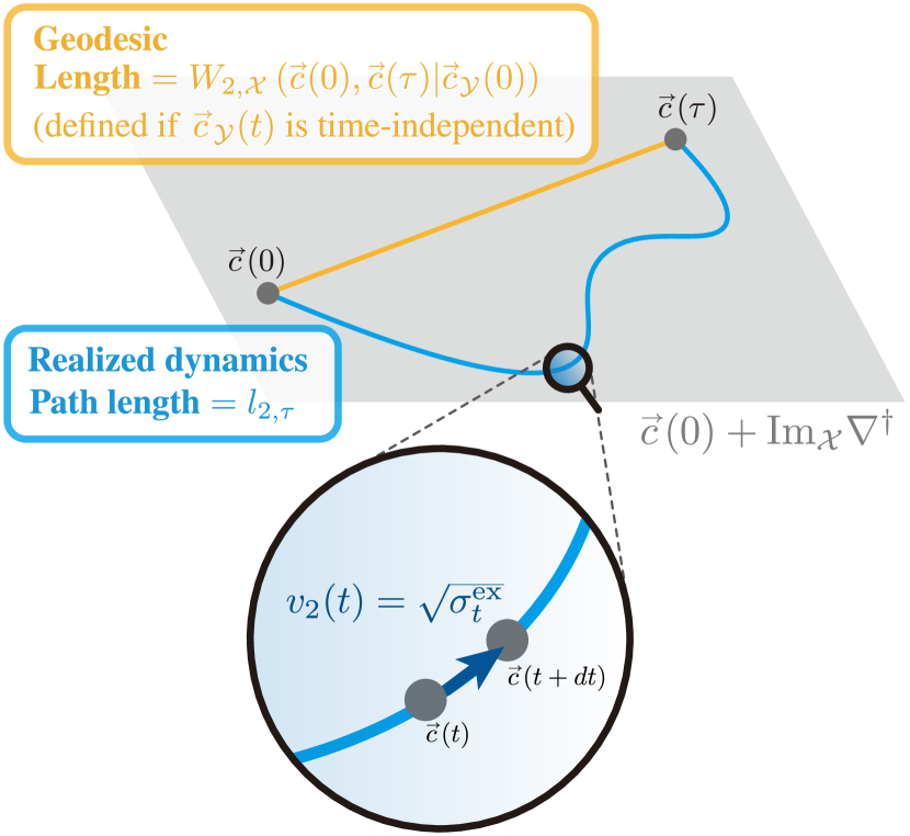
Figure 8: Schematic illustration of the relation between the $2$-Wasserstein distance and the excess EPR. The trajectory of the realized dynamics during the period $[0,\tau]$ (light-blue curve) is a curve with length $l_{2,\tau}$ on the stoichiometric manifold $\mathchoice{\kern-0.15pt\overset{\kern 0.7pt\smash{\lower 1.07639pt\hbox{\scalebox{0.45}{$\bm{\rightarrow}$}}}\kern-0.3pt}{c}}{\kern-0.15pt\overset{\kern 0.7pt\smash{\lower 1.07639pt\hbox{\scalebox{0.45}{$\bm{\rightarrow}$}}}\kern-0.3pt}{c}}{\overset{\smash{\lower 0.6458pt\hbox{\kern 0.2pt\scalebox{0.3}{$\bm{\rightarrow}$}\kern-0.8pt}}}{c}}{\overset{\smash{\lower 0.6458pt\hbox{\kern 0.2pt\scalebox{0.3}{$\bm{\rightarrow}$}\kern-0.8pt}}}{c}}(0)+\mathrm{Im}_{\mathcal{X}}\nabla^{{\dagger}}$ (gray space). We can define the geodesic between the initial and final concentration distributions, $\mathchoice{\kern-0.15pt\overset{\kern 0.7pt\smash{\lower 1.07639pt\hbox{\scalebox{0.45}{$\bm{\rightarrow}$}}}\kern-0.3pt}{c}}{\kern-0.15pt\overset{\kern 0.7pt\smash{\lower 1.07639pt\hbox{\scalebox{0.45}{$\bm{\rightarrow}$}}}\kern-0.3pt}{c}}{\overset{\smash{\lower 0.6458pt\hbox{\kern 0.2pt\scalebox{0.3}{$\bm{\rightarrow}$}\kern-0.8pt}}}{c}}{\overset{\smash{\lower 0.6458pt\hbox{\kern 0.2pt\scalebox{0.3}{$\bm{\rightarrow}$}\kern-0.8pt}}}{c}}(0)$ and $\mathchoice{\kern-0.15pt\overset{\kern 0.7pt\smash{\lower 1.07639pt\hbox{\scalebox{0.45}{$\bm{\rightarrow}$}}}\kern-0.3pt}{c}}{\kern-0.15pt\overset{\kern 0.7pt\smash{\lower 1.07639pt\hbox{\scalebox{0.45}{$\bm{\rightarrow}$}}}\kern-0.3pt}{c}}{\overset{\smash{\lower 0.6458pt\hbox{\kern 0.2pt\scalebox{0.3}{$\bm{\rightarrow}$}\kern-0.8pt}}}{c}}{\overset{\smash{\lower 0.6458pt\hbox{\kern 0.2pt\scalebox{0.3}{$\bm{\rightarrow}$}\kern-0.8pt}}}{c}}(\tau)$ (yellow line) if the concentrations of the external species are constant in time as $\mathchoice{\kern-0.15pt\overset{\kern 0.7pt\smash{\lower 1.07639pt\hbox{\scalebox{0.45}{$\bm{\rightarrow}$}}}\kern-0.3pt}{c}}{\kern-0.15pt\overset{\kern 0.7pt\smash{\lower 1.07639pt\hbox{\scalebox{0.45}{$\bm{\rightarrow}$}}}\kern-0.3pt}{c}}{\overset{\smash{\lower 0.6458pt\hbox{\kern 0.2pt\scalebox{0.3}{$\bm{\rightarrow}$}\kern-0.8pt}}}{c}}{\overset{\smash{\lower 0.6458pt\hbox{\kern 0.2pt\scalebox{0.3}{$\bm{\rightarrow}$}\kern-0.8pt}}}{c}}_{\mathcal{Y}}(t)=\mathchoice{\kern-0.15pt\overset{\kern 0.7pt\smash{\lower 1.07639pt\hbox{\scalebox{0.45}{$\bm{\rightarrow}$}}}\kern-0.3pt}{c}}{\kern-0.15pt\overset{\kern 0.7pt\smash{\lower 1.07639pt\hbox{\scalebox{0.45}{$\bm{\rightarrow}$}}}\kern-0.3pt}{c}}{\overset{\smash{\lower 0.6458pt\hbox{\kern 0.2pt\scalebox{0.3}{$\bm{\rightarrow}$}\kern-0.8pt}}}{c}}{\overset{\smash{\lower 0.6458pt\hbox{\kern 0.2pt\scalebox{0.3}{$\bm{\rightarrow}$}\kern-0.8pt}}}{c}}_{\mathcal{Y}}(0)$. The geodesic also lies on the stoichiometric manifold and has length ${W}_{2,\mathcal{X}}\quantity(\mathchoice{\kern-0.15pt\overset{\kern 0.7pt\smash{\lower 1.07639pt\hbox{\scalebox{0.45}{$\bm{\rightarrow}$}}}\kern-0.3pt}{c}}{\kern-0.15pt\overset{\kern 0.7pt\smash{\lower 1.07639pt\hbox{\scalebox{0.45}{$\bm{\rightarrow}$}}}\kern-0.3pt}{c}}{\overset{\smash{\lower 0.6458pt\hbox{\kern 0.2pt\scalebox{0.3}{$\bm{\rightarrow}$}\kern-0.8pt}}}{c}}{\overset{\smash{\lower 0.6458pt\hbox{\kern 0.2pt\scalebox{0.3}{$\bm{\rightarrow}$}\kern-0.8pt}}}{c}}(0),\mathchoice{\kern-0.15pt\overset{\kern 0.7pt\smash{\lower 1.07639pt\hbox{\scalebox{0.45}{$\bm{\rightarrow}$}}}\kern-0.3pt}{c}}{\kern-0.15pt\overset{\kern 0.7pt\smash{\lower 1.07639pt\hbox{\scalebox{0.45}{$\bm{\rightarrow}$}}}\kern-0.3pt}{c}}{\overset{\smash{\lower 0.6458pt\hbox{\kern 0.2pt\scalebox{0.3}{$\bm{\rightarrow}$}\kern-0.8pt}}}{c}}{\overset{\smash{\lower 0.6458pt\hbox{\kern 0.2pt\scalebox{0.3}{$\bm{\rightarrow}$}\kern-0.8pt}}}{c}}(\tau)|\mathchoice{\kern-0.15pt\overset{\kern 0.7pt\smash{\lower 1.07639pt\hbox{\scalebox{0.45}{$\bm{\rightarrow}$}}}\kern-0.3pt}{c}}{\kern-0.15pt\overset{\kern 0.7pt\smash{\lower 1.07639pt\hbox{\scalebox{0.45}{$\bm{\rightarrow}$}}}\kern-0.3pt}{c}}{\overset{\smash{\lower 0.6458pt\hbox{\kern 0.2pt\scalebox{0.3}{$\bm{\rightarrow}$}\kern-0.8pt}}}{c}}{\overset{\smash{\lower 0.6458pt\hbox{\kern 0.2pt\scalebox{0.3}{$\bm{\rightarrow}$}\kern-0.8pt}}}{c}}_{\mathcal{Y}}(0))$. The speed of the concentration distribution moving on the stoichiometric manifold $v_{2}(t)$ equals the square root of the excess EPR, $\sqrt{\sigma^{\mathrm{ex}}_{t}}$.

This relation between the speed of the dynamics and the excess EPR leads to the series of TSLs,

$$l_{2,\tau}^{2}\leq\tau\Sigma_{\tau}^{\mathrm{ex}}\leq\tau\Sigma_{\tau}.$$ (166)

The first inequality is derived from the Cauchy–Schwarz inequality $\quantity[\int_{0}^{\tau}dtv_{2}(t)]^{2}\leq\quantity[\int_{0}^{\tau}dt]\quantity[\int_{0}^{\tau}dtv_{2}(t)^{2}]$ and the property of the excess EPR in Eq. (162). If we consider the system where the concentrations of all the external species are constant in time as $\mathchoice{\kern-0.15pt\overset{\kern 0.7pt\smash{\lower 1.07639pt\hbox{\scalebox{0.45}{$\bm{\rightarrow}$}}}\kern-0.3pt}{c}}{\kern-0.15pt\overset{\kern 0.7pt\smash{\lower 1.07639pt\hbox{\scalebox{0.45}{$\bm{\rightarrow}$}}}\kern-0.3pt}{c}}{\overset{\smash{\lower 0.6458pt\hbox{\kern 0.2pt\scalebox{0.3}{$\bm{\rightarrow}$}\kern-0.8pt}}}{c}}{\overset{\smash{\lower 0.6458pt\hbox{\kern 0.2pt\scalebox{0.3}{$\bm{\rightarrow}$}\kern-0.8pt}}}{c}}_{\mathcal{Y}}(t)=\mathchoice{\kern-0.15pt\overset{\kern 0.7pt\smash{\lower 1.07639pt\hbox{\scalebox{0.45}{$\bm{\rightarrow}$}}}\kern-0.3pt}{c}}{\kern-0.15pt\overset{\kern 0.7pt\smash{\lower 1.07639pt\hbox{\scalebox{0.45}{$\bm{\rightarrow}$}}}\kern-0.3pt}{c}}{\overset{\smash{\lower 0.6458pt\hbox{\kern 0.2pt\scalebox{0.3}{$\bm{\rightarrow}$}\kern-0.8pt}}}{c}}{\overset{\smash{\lower 0.6458pt\hbox{\kern 0.2pt\scalebox{0.3}{$\bm{\rightarrow}$}\kern-0.8pt}}}{c}}_{\mathcal{Y}}(0)$, and $\mathcal{M}$ depends on time through only $\mathchoice{\kern-0.15pt\overset{\kern 0.7pt\smash{\lower 1.07639pt\hbox{\scalebox{0.45}{$\bm{\rightarrow}$}}}\kern-0.3pt}{c}}{\kern-0.15pt\overset{\kern 0.7pt\smash{\lower 1.07639pt\hbox{\scalebox{0.45}{$\bm{\rightarrow}$}}}\kern-0.3pt}{c}}{\overset{\smash{\lower 0.6458pt\hbox{\kern 0.2pt\scalebox{0.3}{$\bm{\rightarrow}$}\kern-0.8pt}}}{c}}{\overset{\smash{\lower 0.6458pt\hbox{\kern 0.2pt\scalebox{0.3}{$\bm{\rightarrow}$}\kern-0.8pt}}}{c}}$, we also obtain

$${W}_{2,\mathcal{X}}(\mathchoice{\kern-0.15pt\overset{\kern 0.7pt\smash{\lower 1.07639pt\hbox{\scalebox{0.45}{$\bm{\rightarrow}$}}}\kern-0.3pt}{c}}{\kern-0.15pt\overset{\kern 0.7pt\smash{\lower 1.07639pt\hbox{\scalebox{0.45}{$\bm{\rightarrow}$}}}\kern-0.3pt}{c}}{\overset{\smash{\lower 0.6458pt\hbox{\kern 0.2pt\scalebox{0.3}{$\bm{\rightarrow}$}\kern-0.8pt}}}{c}}{\overset{\smash{\lower 0.6458pt\hbox{\kern 0.2pt\scalebox{0.3}{$\bm{\rightarrow}$}\kern-0.8pt}}}{c}}(0),\mathchoice{\kern-0.15pt\overset{\kern 0.7pt\smash{\lower 1.07639pt\hbox{\scalebox{0.45}{$\bm{\rightarrow}$}}}\kern-0.3pt}{c}}{\kern-0.15pt\overset{\kern 0.7pt\smash{\lower 1.07639pt\hbox{\scalebox{0.45}{$\bm{\rightarrow}$}}}\kern-0.3pt}{c}}{\overset{\smash{\lower 0.6458pt\hbox{\kern 0.2pt\scalebox{0.3}{$\bm{\rightarrow}$}\kern-0.8pt}}}{c}}{\overset{\smash{\lower 0.6458pt\hbox{\kern 0.2pt\scalebox{0.3}{$\bm{\rightarrow}$}\kern-0.8pt}}}{c}}(\tau)|\mathchoice{\kern-0.15pt\overset{\kern 0.7pt\smash{\lower 1.07639pt\hbox{\scalebox{0.45}{$\bm{\rightarrow}$}}}\kern-0.3pt}{c}}{\kern-0.15pt\overset{\kern 0.7pt\smash{\lower 1.07639pt\hbox{\scalebox{0.45}{$\bm{\rightarrow}$}}}\kern-0.3pt}{c}}{\overset{\smash{\lower 0.6458pt\hbox{\kern 0.2pt\scalebox{0.3}{$\bm{\rightarrow}$}\kern-0.8pt}}}{c}}{\overset{\smash{\lower 0.6458pt\hbox{\kern 0.2pt\scalebox{0.3}{$\bm{\rightarrow}$}\kern-0.8pt}}}{c}}_{\mathcal{Y}}(0))^{2}\leq l_{2,\tau}^{2}\leq\tau\Sigma_{\tau}^{\mathrm{ex}}\leq\tau\Sigma_{\tau}.$$ (167)

The first inequality is a consequence of the triangle inequality for the $2$-Wasserstein distance, which is proved in Appendix E.5. We remark that the TSL with $l_{2,\tau}$ is tighter than the one with ${W}_{2,\mathcal{X}}$ reflecting the fact that the path $\{\mathchoice{\kern-0.15pt\overset{\kern 0.7pt\smash{\lower 1.07639pt\hbox{\scalebox{0.45}{$\bm{\rightarrow}$}}}\kern-0.3pt}{c}}{\kern-0.15pt\overset{\kern 0.7pt\smash{\lower 1.07639pt\hbox{\scalebox{0.45}{$\bm{\rightarrow}$}}}\kern-0.3pt}{c}}{\overset{\smash{\lower 0.6458pt\hbox{\kern 0.2pt\scalebox{0.3}{$\bm{\rightarrow}$}\kern-0.8pt}}}{c}}{\overset{\smash{\lower 0.6458pt\hbox{\kern 0.2pt\scalebox{0.3}{$\bm{\rightarrow}$}\kern-0.8pt}}}{c}}_{\mathcal{X}}\}_{t\in[0,\tau]}$ is generally not the geodesic, whose length is ${W}_{2,\mathcal{X}}$.

These TSLs for RDSs imply a trade-off between the dissipation due to pattern formation and the change speed of the pattern because the TSL in Eq. (167) is rewritten as $(l_{2,\tau}/\tau)^{2}\leq(\Sigma_{\tau}^{\mathrm{ex}}/\tau)$, where $l_{2,\tau}/\tau$ means the change speed from the initial pattern at $t=0$ to the final pattern at $t=\tau$, and $\Sigma_{\tau}^{\mathrm{ex}}/\tau=\langle\sigma^{\mathrm{ex}}\rangle_{\tau}$ means the time average of dissipation due to the time evolution of the pattern. This trade-off relation means that the slower the speed of pattern formation, the smaller the dissipation can be.

We also obtain TSLs based on the $1$-Wasserstein distance. Similarly to Eq. (160), we define the path length between the initial and final distribution with the $1$-Wasserstein distance as

$$l_{1,\tau}\coloneqq\int_{0}^{\tau}dt\,v_{1}(t),$$ (168)

where the integrand $v_{1}(t)$ indicates the speed of dynamics measured with ${W}_{1,\mathcal{X}}$,

$$v_{1}(t)\coloneqq\lim_{\varDelta t\to 0}\frac{{W}_{1,\mathcal{X}}(\mathchoice{\kern-0.15pt\overset{\kern 0.7pt\smash{\lower 1.07639pt\hbox{\scalebox{0.45}{$\bm{\rightarrow}$}}}\kern-0.3pt}{c}}{\kern-0.15pt\overset{\kern 0.7pt\smash{\lower 1.07639pt\hbox{\scalebox{0.45}{$\bm{\rightarrow}$}}}\kern-0.3pt}{c}}{\overset{\smash{\lower 0.6458pt\hbox{\kern 0.2pt\scalebox{0.3}{$\bm{\rightarrow}$}\kern-0.8pt}}}{c}}{\overset{\smash{\lower 0.6458pt\hbox{\kern 0.2pt\scalebox{0.3}{$\bm{\rightarrow}$}\kern-0.8pt}}}{c}}(t),\mathchoice{\kern-0.15pt\overset{\kern 0.7pt\smash{\lower 1.07639pt\hbox{\scalebox{0.45}{$\bm{\rightarrow}$}}}\kern-0.3pt}{c}}{\kern-0.15pt\overset{\kern 0.7pt\smash{\lower 1.07639pt\hbox{\scalebox{0.45}{$\bm{\rightarrow}$}}}\kern-0.3pt}{c}}{\overset{\smash{\lower 0.6458pt\hbox{\kern 0.2pt\scalebox{0.3}{$\bm{\rightarrow}$}\kern-0.8pt}}}{c}}{\overset{\smash{\lower 0.6458pt\hbox{\kern 0.2pt\scalebox{0.3}{$\bm{\rightarrow}$}\kern-0.8pt}}}{c}}(t+\varDelta t))}{\varDelta t}.$$ (169)

The inequality between the $1$- and $2$-Wasserstein distances [Eq. (157)] and this speed $v_{1}$ provide a lower bound of the excess EPR,

$$\sigma_{t}^{\mathrm{ex}}=v_{2}(t)^{2}\geq\frac{v_{1}(t)^{2}}{A_{\mathcal{X}}\quantity[\mathchoice{\kern-0.15pt\overset{\kern 0.7pt\smash{\lower 1.07639pt\hbox{\scalebox{0.45}{$\bm{\rightarrow}$}}}\kern-0.3pt}{c}}{\kern-0.15pt\overset{\kern 0.7pt\smash{\lower 1.07639pt\hbox{\scalebox{0.45}{$\bm{\rightarrow}$}}}\kern-0.3pt}{c}}{\overset{\smash{\lower 0.6458pt\hbox{\kern 0.2pt\scalebox{0.3}{$\bm{\rightarrow}$}\kern-0.8pt}}}{c}}{\overset{\smash{\lower 0.6458pt\hbox{\kern 0.2pt\scalebox{0.3}{$\bm{\rightarrow}$}\kern-0.8pt}}}{c}}(t)]},$$ (170)

where $A_{\mathcal{X}}$ is the functional defined in Eq. (155), representing the intensity of reaction and diffusion. This inequality further leads to the TSLs based on the $1$-Wasserstein distance

$$\frac{{W}_{1,\mathcal{X}}\quantity(\mathchoice{\kern-0.15pt\overset{\kern 0.7pt\smash{\lower 1.07639pt\hbox{\scalebox{0.45}{$\bm{\rightarrow}$}}}\kern-0.3pt}{c}}{\kern-0.15pt\overset{\kern 0.7pt\smash{\lower 1.07639pt\hbox{\scalebox{0.45}{$\bm{\rightarrow}$}}}\kern-0.3pt}{c}}{\overset{\smash{\lower 0.6458pt\hbox{\kern 0.2pt\scalebox{0.3}{$\bm{\rightarrow}$}\kern-0.8pt}}}{c}}{\overset{\smash{\lower 0.6458pt\hbox{\kern 0.2pt\scalebox{0.3}{$\bm{\rightarrow}$}\kern-0.8pt}}}{c}}(0),\mathchoice{\kern-0.15pt\overset{\kern 0.7pt\smash{\lower 1.07639pt\hbox{\scalebox{0.45}{$\bm{\rightarrow}$}}}\kern-0.3pt}{c}}{\kern-0.15pt\overset{\kern 0.7pt\smash{\lower 1.07639pt\hbox{\scalebox{0.45}{$\bm{\rightarrow}$}}}\kern-0.3pt}{c}}{\overset{\smash{\lower 0.6458pt\hbox{\kern 0.2pt\scalebox{0.3}{$\bm{\rightarrow}$}\kern-0.8pt}}}{c}}{\overset{\smash{\lower 0.6458pt\hbox{\kern 0.2pt\scalebox{0.3}{$\bm{\rightarrow}$}\kern-0.8pt}}}{c}}(\tau))^{2}}{\left\langle A_{\mathcal{X}}\quantity[\mathchoice{\kern-0.15pt\overset{\kern 0.7pt\smash{\lower 1.07639pt\hbox{\scalebox{0.45}{$\bm{\rightarrow}$}}}\kern-0.3pt}{c}}{\kern-0.15pt\overset{\kern 0.7pt\smash{\lower 1.07639pt\hbox{\scalebox{0.45}{$\bm{\rightarrow}$}}}\kern-0.3pt}{c}}{\overset{\smash{\lower 0.6458pt\hbox{\kern 0.2pt\scalebox{0.3}{$\bm{\rightarrow}$}\kern-0.8pt}}}{c}}{\overset{\smash{\lower 0.6458pt\hbox{\kern 0.2pt\scalebox{0.3}{$\bm{\rightarrow}$}\kern-0.8pt}}}{c}}]\right\rangle_{\tau}}\leq\frac{l_{1,\tau}^{2}}{\left\langle A_{\mathcal{X}}\quantity[\mathchoice{\kern-0.15pt\overset{\kern 0.7pt\smash{\lower 1.07639pt\hbox{\scalebox{0.45}{$\bm{\rightarrow}$}}}\kern-0.3pt}{c}}{\kern-0.15pt\overset{\kern 0.7pt\smash{\lower 1.07639pt\hbox{\scalebox{0.45}{$\bm{\rightarrow}$}}}\kern-0.3pt}{c}}{\overset{\smash{\lower 0.6458pt\hbox{\kern 0.2pt\scalebox{0.3}{$\bm{\rightarrow}$}\kern-0.8pt}}}{c}}{\overset{\smash{\lower 0.6458pt\hbox{\kern 0.2pt\scalebox{0.3}{$\bm{\rightarrow}$}\kern-0.8pt}}}{c}}]\right\rangle_{\tau}}\leq\tau\Sigma_{\tau}^{\mathrm{ex}}\leq\tau\Sigma_{\tau}.$$ (171)

These TSLs generalize those obtained for MJPs [41, 40] to RDSs and tighten them by using the line length $l_{1,\tau}$ instead of the $1$-Wasserstein distance. We can make the speed limits tighter by replacing $A_{\mathcal{X}}\quantity[\mathchoice{\kern-0.15pt\overset{\kern 0.7pt\smash{\lower 1.07639pt\hbox{\scalebox{0.45}{$\bm{\rightarrow}$}}}\kern-0.3pt}{c}}{\kern-0.15pt\overset{\kern 0.7pt\smash{\lower 1.07639pt\hbox{\scalebox{0.45}{$\bm{\rightarrow}$}}}\kern-0.3pt}{c}}{\overset{\smash{\lower 0.6458pt\hbox{\kern 0.2pt\scalebox{0.3}{$\bm{\rightarrow}$}\kern-0.8pt}}}{c}}{\overset{\smash{\lower 0.6458pt\hbox{\kern 0.2pt\scalebox{0.3}{$\bm{\rightarrow}$}\kern-0.8pt}}}{c}}(t)]$ in Eq. (170) and Eq. (171) with $A^{\prime}_{\mathcal{X}}$ if the mobility tensor satisfies Eq. (60), as we did in Eq. (157). We provide the derivations of these speed limits [Eq. (170), Eq. (171)] in Appendix E.7.

We can consider the leftmost term in Eq. (171) even when the concentration distribution of the external species depends on time and $\mathcal{M}$ explicitly depends on time because we do not need the concentration distribution of the external species and $\mathcal{M}$ to compute the $1$-Wasserstein distance. As in the case of the $2$-Wasserstein distance, the TSL with $l_{1,\tau}$ is tighter than the one with ${W}_{1,\mathcal{X}}$ reflecting the fact that the path $\{\mathchoice{\kern-0.15pt\overset{\kern 0.7pt\smash{\lower 1.07639pt\hbox{\scalebox{0.45}{$\bm{\rightarrow}$}}}\kern-0.3pt}{c}}{\kern-0.15pt\overset{\kern 0.7pt\smash{\lower 1.07639pt\hbox{\scalebox{0.45}{$\bm{\rightarrow}$}}}\kern-0.3pt}{c}}{\overset{\smash{\lower 0.6458pt\hbox{\kern 0.2pt\scalebox{0.3}{$\bm{\rightarrow}$}\kern-0.8pt}}}{c}}{\overset{\smash{\lower 0.6458pt\hbox{\kern 0.2pt\scalebox{0.3}{$\bm{\rightarrow}$}\kern-0.8pt}}}{c}}_{\mathcal{X}}\}_{t\in[0,\tau]}$ is generally not the geodesic, whose length is ${W}_{1,\mathcal{X}}$.

We can rewrite the TSL $l_{1,\tau}^{2}/\langle A_{\mathcal{X}}\rangle_{\tau}\leq\tau\Sigma^{\mathrm{ex}}_{\tau}$ in Eq. (171) as $[(l_{1,\tau}/\tau)^{2}/\langle A_{\mathcal{X}}\rangle_{\tau}]\leq(\Sigma^{\mathrm{ex}}_{\tau}/\tau)$, where $l_{1,\tau}/\tau$ is the change speed of the pattern measured with the $1$-Wasserstein distance, and $\langle A_{\mathcal{X}}\rangle_{\tau}$ indicates time average of intensities of reactions and diffusive dynamics. This rewrite allows us to regard the TSLs as trade-off relations between the dissipation due to pattern formation, change speed of pattern, and intensities of reactions and diffusive dynamics: the slower the speed of the pattern or the higher intensities of reactions and diffusive dynamics, the smaller the dissipation can be.

It is not obvious which lower bound of $\tau\Sigma^{\mathrm{ex}}_{\tau}$ is tighter: ${W}_{2,\mathcal{X}}(\mathchoice{\kern-0.15pt\overset{\kern 0.7pt\smash{\lower 1.07639pt\hbox{\scalebox{0.45}{$\bm{\rightarrow}$}}}\kern-0.3pt}{c}}{\kern-0.15pt\overset{\kern 0.7pt\smash{\lower 1.07639pt\hbox{\scalebox{0.45}{$\bm{\rightarrow}$}}}\kern-0.3pt}{c}}{\overset{\smash{\lower 0.6458pt\hbox{\kern 0.2pt\scalebox{0.3}{$\bm{\rightarrow}$}\kern-0.8pt}}}{c}}{\overset{\smash{\lower 0.6458pt\hbox{\kern 0.2pt\scalebox{0.3}{$\bm{\rightarrow}$}\kern-0.8pt}}}{c}}(0),\mathchoice{\kern-0.15pt\overset{\kern 0.7pt\smash{\lower 1.07639pt\hbox{\scalebox{0.45}{$\bm{\rightarrow}$}}}\kern-0.3pt}{c}}{\kern-0.15pt\overset{\kern 0.7pt\smash{\lower 1.07639pt\hbox{\scalebox{0.45}{$\bm{\rightarrow}$}}}\kern-0.3pt}{c}}{\overset{\smash{\lower 0.6458pt\hbox{\kern 0.2pt\scalebox{0.3}{$\bm{\rightarrow}$}\kern-0.8pt}}}{c}}{\overset{\smash{\lower 0.6458pt\hbox{\kern 0.2pt\scalebox{0.3}{$\bm{\rightarrow}$}\kern-0.8pt}}}{c}}(\tau)|\mathchoice{\kern-0.15pt\overset{\kern 0.7pt\smash{\lower 1.07639pt\hbox{\scalebox{0.45}{$\bm{\rightarrow}$}}}\kern-0.3pt}{c}}{\kern-0.15pt\overset{\kern 0.7pt\smash{\lower 1.07639pt\hbox{\scalebox{0.45}{$\bm{\rightarrow}$}}}\kern-0.3pt}{c}}{\overset{\smash{\lower 0.6458pt\hbox{\kern 0.2pt\scalebox{0.3}{$\bm{\rightarrow}$}\kern-0.8pt}}}{c}}{\overset{\smash{\lower 0.6458pt\hbox{\kern 0.2pt\scalebox{0.3}{$\bm{\rightarrow}$}\kern-0.8pt}}}{c}}_{\mathcal{Y}}(0))^{2}$ in Eq. (167) or $W_{1,\mathcal{X}}(\mathchoice{\kern-0.15pt\overset{\kern 0.7pt\smash{\lower 1.07639pt\hbox{\scalebox{0.45}{$\bm{\rightarrow}$}}}\kern-0.3pt}{c}}{\kern-0.15pt\overset{\kern 0.7pt\smash{\lower 1.07639pt\hbox{\scalebox{0.45}{$\bm{\rightarrow}$}}}\kern-0.3pt}{c}}{\overset{\smash{\lower 0.6458pt\hbox{\kern 0.2pt\scalebox{0.3}{$\bm{\rightarrow}$}\kern-0.8pt}}}{c}}{\overset{\smash{\lower 0.6458pt\hbox{\kern 0.2pt\scalebox{0.3}{$\bm{\rightarrow}$}\kern-0.8pt}}}{c}}(0),\mathchoice{\kern-0.15pt\overset{\kern 0.7pt\smash{\lower 1.07639pt\hbox{\scalebox{0.45}{$\bm{\rightarrow}$}}}\kern-0.3pt}{c}}{\kern-0.15pt\overset{\kern 0.7pt\smash{\lower 1.07639pt\hbox{\scalebox{0.45}{$\bm{\rightarrow}$}}}\kern-0.3pt}{c}}{\overset{\smash{\lower 0.6458pt\hbox{\kern 0.2pt\scalebox{0.3}{$\bm{\rightarrow}$}\kern-0.8pt}}}{c}}{\overset{\smash{\lower 0.6458pt\hbox{\kern 0.2pt\scalebox{0.3}{$\bm{\rightarrow}$}\kern-0.8pt}}}{c}}(\tau))^{2}/\langle A_{\mathcal{X}}[\mathchoice{\kern-0.15pt\overset{\kern 0.7pt\smash{\lower 1.07639pt\hbox{\scalebox{0.45}{$\bm{\rightarrow}$}}}\kern-0.3pt}{c}}{\kern-0.15pt\overset{\kern 0.7pt\smash{\lower 1.07639pt\hbox{\scalebox{0.45}{$\bm{\rightarrow}$}}}\kern-0.3pt}{c}}{\overset{\smash{\lower 0.6458pt\hbox{\kern 0.2pt\scalebox{0.3}{$\bm{\rightarrow}$}\kern-0.8pt}}}{c}}{\overset{\smash{\lower 0.6458pt\hbox{\kern 0.2pt\scalebox{0.3}{$\bm{\rightarrow}$}\kern-0.8pt}}}{c}}]\rangle_{\tau}$ in Eq. (171). This is because the argument of the denominator in the left-hand side of the inequality between ${W}_{1,\mathcal{X}}$ and ${W}_{2,\mathcal{X}}$ [Eq. (157)] and that of the TSL with ${W}_{1,\mathcal{X}}$ [Eq. (171)] are different: the former is the optimal time series of concentration distributions for the $2$-Wasserstein distance, $\mathchoice{\kern-0.15pt\overset{\kern 0.7pt\smash{\lower 1.07639pt\hbox{\scalebox{0.45}{$\bm{\rightarrow}$}}}\kern-0.3pt}{c}}{\kern-0.15pt\overset{\kern 0.7pt\smash{\lower 1.07639pt\hbox{\scalebox{0.45}{$\bm{\rightarrow}$}}}\kern-0.3pt}{c}}{\overset{\smash{\lower 0.6458pt\hbox{\kern 0.2pt\scalebox{0.3}{$\bm{\rightarrow}$}\kern-0.8pt}}}{c}}{\overset{\smash{\lower 0.6458pt\hbox{\kern 0.2pt\scalebox{0.3}{$\bm{\rightarrow}$}\kern-0.8pt}}}{c}}^{\star}$, while the latter is the original time series, $\mathchoice{\kern-0.15pt\overset{\kern 0.7pt\smash{\lower 1.07639pt\hbox{\scalebox{0.45}{$\bm{\rightarrow}$}}}\kern-0.3pt}{c}}{\kern-0.15pt\overset{\kern 0.7pt\smash{\lower 1.07639pt\hbox{\scalebox{0.45}{$\bm{\rightarrow}$}}}\kern-0.3pt}{c}}{\overset{\smash{\lower 0.6458pt\hbox{\kern 0.2pt\scalebox{0.3}{$\bm{\rightarrow}$}\kern-0.8pt}}}{c}}{\overset{\smash{\lower 0.6458pt\hbox{\kern 0.2pt\scalebox{0.3}{$\bm{\rightarrow}$}\kern-0.8pt}}}{c}}$. Similarly, it is not clear which lower bound is tighter: $l_{2,\tau}^{2}$ in Eq. (167) or $l_{1,\tau}^{2}/\langle A_{\mathcal{X}}[\mathchoice{\kern-0.15pt\overset{\kern 0.7pt\smash{\lower 1.07639pt\hbox{\scalebox{0.45}{$\bm{\rightarrow}$}}}\kern-0.3pt}{c}}{\kern-0.15pt\overset{\kern 0.7pt\smash{\lower 1.07639pt\hbox{\scalebox{0.45}{$\bm{\rightarrow}$}}}\kern-0.3pt}{c}}{\overset{\smash{\lower 0.6458pt\hbox{\kern 0.2pt\scalebox{0.3}{$\bm{\rightarrow}$}\kern-0.8pt}}}{c}}{\overset{\smash{\lower 0.6458pt\hbox{\kern 0.2pt\scalebox{0.3}{$\bm{\rightarrow}$}\kern-0.8pt}}}{c}}]\rangle_{\tau}$ in Eq. (171) (see also Appendix E.7).

V.5 Numerical examples: thermodynamic speed limits

We show numerical results for the $1$-Wasserstein distance and the TSLs [Eqs. (171) and (166)] by using the two systems, the Fisher–KPP equation and the Brusselator model, shown in Sec. IV.3. We use $A^{\prime}_{\mathcal{X}}$ [Eq. (159)] (not $A_{\mathcal{X}}$) because these systems have the simple mobility tensor in Eq. (60). Here, we do not treat the $2$-Wasserstein distance due to its computational complexity. We use the primal-dual algorithm [82, 83] to compute the $1$-Wasserstein distance. To compare with the behavior of ${W}_{1,\mathcal{X}}$, we use the $L^{1}$ distance between concentration distributions of the internal species,

$${L}_{\mathcal{X}}(\mathchoice{\kern-0.15pt\overset{\kern 0.7pt\smash{\lower 1.07639pt\hbox{\scalebox{0.45}{$\bm{\rightarrow}$}}}\kern-0.3pt}{c}}{\kern-0.15pt\overset{\kern 0.7pt\smash{\lower 1.07639pt\hbox{\scalebox{0.45}{$\bm{\rightarrow}$}}}\kern-0.3pt}{c}}{\overset{\smash{\lower 0.6458pt\hbox{\kern 0.2pt\scalebox{0.3}{$\bm{\rightarrow}$}\kern-0.8pt}}}{c}}{\overset{\smash{\lower 0.6458pt\hbox{\kern 0.2pt\scalebox{0.3}{$\bm{\rightarrow}$}\kern-0.8pt}}}{c}}(0),\mathchoice{\kern-0.15pt\overset{\kern 0.7pt\smash{\lower 1.07639pt\hbox{\scalebox{0.45}{$\bm{\rightarrow}$}}}\kern-0.3pt}{c}}{\kern-0.15pt\overset{\kern 0.7pt\smash{\lower 1.07639pt\hbox{\scalebox{0.45}{$\bm{\rightarrow}$}}}\kern-0.3pt}{c}}{\overset{\smash{\lower 0.6458pt\hbox{\kern 0.2pt\scalebox{0.3}{$\bm{\rightarrow}$}\kern-0.8pt}}}{c}}{\overset{\smash{\lower 0.6458pt\hbox{\kern 0.2pt\scalebox{0.3}{$\bm{\rightarrow}$}\kern-0.8pt}}}{c}}(\tau))\coloneqq\sum_{\alpha\in\mathcal{X}}\int_{V}d\bm{r}\left|c_{\alpha}(\bm{r};\tau)-c_{\alpha}(\bm{r};0)\right|,$$ (172)

and the $L^{1}$ distance between total concentrations of the internal species,

$${L}_{\mathcal{X}}^{\mathrm{tot}}(\mathchoice{\kern-0.15pt\overset{\kern 0.7pt\smash{\lower 1.07639pt\hbox{\scalebox{0.45}{$\bm{\rightarrow}$}}}\kern-0.3pt}{c}}{\kern-0.15pt\overset{\kern 0.7pt\smash{\lower 1.07639pt\hbox{\scalebox{0.45}{$\bm{\rightarrow}$}}}\kern-0.3pt}{c}}{\overset{\smash{\lower 0.6458pt\hbox{\kern 0.2pt\scalebox{0.3}{$\bm{\rightarrow}$}\kern-0.8pt}}}{c}}{\overset{\smash{\lower 0.6458pt\hbox{\kern 0.2pt\scalebox{0.3}{$\bm{\rightarrow}$}\kern-0.8pt}}}{c}}(0),\mathchoice{\kern-0.15pt\overset{\kern 0.7pt\smash{\lower 1.07639pt\hbox{\scalebox{0.45}{$\bm{\rightarrow}$}}}\kern-0.3pt}{c}}{\kern-0.15pt\overset{\kern 0.7pt\smash{\lower 1.07639pt\hbox{\scalebox{0.45}{$\bm{\rightarrow}$}}}\kern-0.3pt}{c}}{\overset{\smash{\lower 0.6458pt\hbox{\kern 0.2pt\scalebox{0.3}{$\bm{\rightarrow}$}\kern-0.8pt}}}{c}}{\overset{\smash{\lower 0.6458pt\hbox{\kern 0.2pt\scalebox{0.3}{$\bm{\rightarrow}$}\kern-0.8pt}}}{c}}(\tau))\coloneqq\sum_{\alpha\in\mathcal{X}}\left|\int_{V}d\bm{r}\,c_{\alpha}(\bm{r};\tau)-\int_{V}d\bm{r}\,c_{\alpha}(\bm{r};0)\right|.$$ (173)

Note that ${L}_{\mathcal{X}}$ accounts not only for changes in the total concentrations, but also for changes in the shape of the pattern, which is not accounted for in ${L}_{\mathcal{X}}^{\mathrm{tot}}$. The triangle inequality implies ${L}_{\mathcal{X}}(\mathchoice{\kern-0.15pt\overset{\kern 0.7pt\smash{\lower 1.07639pt\hbox{\scalebox{0.45}{$\bm{\rightarrow}$}}}\kern-0.3pt}{c}}{\kern-0.15pt\overset{\kern 0.7pt\smash{\lower 1.07639pt\hbox{\scalebox{0.45}{$\bm{\rightarrow}$}}}\kern-0.3pt}{c}}{\overset{\smash{\lower 0.6458pt\hbox{\kern 0.2pt\scalebox{0.3}{$\bm{\rightarrow}$}\kern-0.8pt}}}{c}}{\overset{\smash{\lower 0.6458pt\hbox{\kern 0.2pt\scalebox{0.3}{$\bm{\rightarrow}$}\kern-0.8pt}}}{c}}(0),\mathchoice{\kern-0.15pt\overset{\kern 0.7pt\smash{\lower 1.07639pt\hbox{\scalebox{0.45}{$\bm{\rightarrow}$}}}\kern-0.3pt}{c}}{\kern-0.15pt\overset{\kern 0.7pt\smash{\lower 1.07639pt\hbox{\scalebox{0.45}{$\bm{\rightarrow}$}}}\kern-0.3pt}{c}}{\overset{\smash{\lower 0.6458pt\hbox{\kern 0.2pt\scalebox{0.3}{$\bm{\rightarrow}$}\kern-0.8pt}}}{c}}{\overset{\smash{\lower 0.6458pt\hbox{\kern 0.2pt\scalebox{0.3}{$\bm{\rightarrow}$}\kern-0.8pt}}}{c}}(\tau))\geq{L}_{\mathcal{X}}^{\mathrm{tot}}(\mathchoice{\kern-0.15pt\overset{\kern 0.7pt\smash{\lower 1.07639pt\hbox{\scalebox{0.45}{$\bm{\rightarrow}$}}}\kern-0.3pt}{c}}{\kern-0.15pt\overset{\kern 0.7pt\smash{\lower 1.07639pt\hbox{\scalebox{0.45}{$\bm{\rightarrow}$}}}\kern-0.3pt}{c}}{\overset{\smash{\lower 0.6458pt\hbox{\kern 0.2pt\scalebox{0.3}{$\bm{\rightarrow}$}\kern-0.8pt}}}{c}}{\overset{\smash{\lower 0.6458pt\hbox{\kern 0.2pt\scalebox{0.3}{$\bm{\rightarrow}$}\kern-0.8pt}}}{c}}(0),\mathchoice{\kern-0.15pt\overset{\kern 0.7pt\smash{\lower 1.07639pt\hbox{\scalebox{0.45}{$\bm{\rightarrow}$}}}\kern-0.3pt}{c}}{\kern-0.15pt\overset{\kern 0.7pt\smash{\lower 1.07639pt\hbox{\scalebox{0.45}{$\bm{\rightarrow}$}}}\kern-0.3pt}{c}}{\overset{\smash{\lower 0.6458pt\hbox{\kern 0.2pt\scalebox{0.3}{$\bm{\rightarrow}$}\kern-0.8pt}}}{c}}{\overset{\smash{\lower 0.6458pt\hbox{\kern 0.2pt\scalebox{0.3}{$\bm{\rightarrow}$}\kern-0.8pt}}}{c}}(\tau))$.

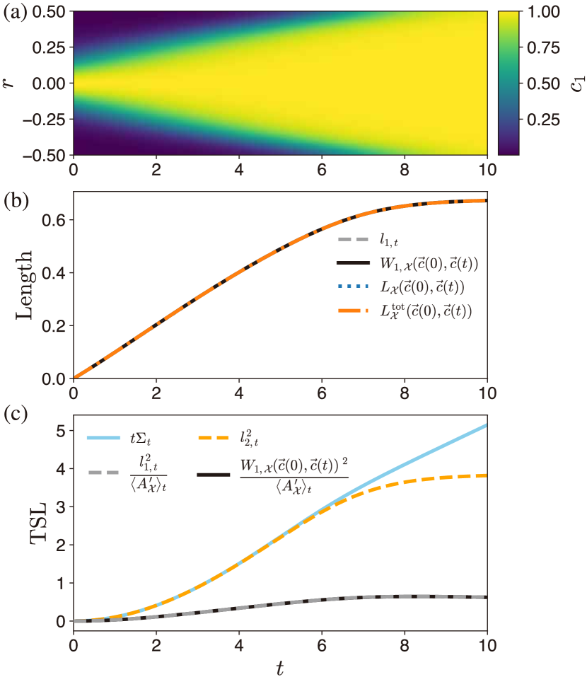
Figure 9: The lengths and the TSLs in the Fisher–KPP equation. (a) The time series of $c_{1}$ (for comparison). The figure is the same as Fig. 5(a). (b) Various lengths between $\mathchoice{\kern-0.15pt\overset{\kern 0.7pt\smash{\lower 1.07639pt\hbox{\scalebox{0.45}{$\bm{\rightarrow}$}}}\kern-0.3pt}{c}}{\kern-0.15pt\overset{\kern 0.7pt\smash{\lower 1.07639pt\hbox{\scalebox{0.45}{$\bm{\rightarrow}$}}}\kern-0.3pt}{c}}{\overset{\smash{\lower 0.6458pt\hbox{\kern 0.2pt\scalebox{0.3}{$\bm{\rightarrow}$}\kern-0.8pt}}}{c}}{\overset{\smash{\lower 0.6458pt\hbox{\kern 0.2pt\scalebox{0.3}{$\bm{\rightarrow}$}\kern-0.8pt}}}{c}}(0)$ and $\mathchoice{\kern-0.15pt\overset{\kern 0.7pt\smash{\lower 1.07639pt\hbox{\scalebox{0.45}{$\bm{\rightarrow}$}}}\kern-0.3pt}{c}}{\kern-0.15pt\overset{\kern 0.7pt\smash{\lower 1.07639pt\hbox{\scalebox{0.45}{$\bm{\rightarrow}$}}}\kern-0.3pt}{c}}{\overset{\smash{\lower 0.6458pt\hbox{\kern 0.2pt\scalebox{0.3}{$\bm{\rightarrow}$}\kern-0.8pt}}}{c}}{\overset{\smash{\lower 0.6458pt\hbox{\kern 0.2pt\scalebox{0.3}{$\bm{\rightarrow}$}\kern-0.8pt}}}{c}}(t)$: $l_{1,t}$ (black line), ${W}_{1,\mathcal{X}}(\mathchoice{\kern-0.15pt\overset{\kern 0.7pt\smash{\lower 1.07639pt\hbox{\scalebox{0.45}{$\bm{\rightarrow}$}}}\kern-0.3pt}{c}}{\kern-0.15pt\overset{\kern 0.7pt\smash{\lower 1.07639pt\hbox{\scalebox{0.45}{$\bm{\rightarrow}$}}}\kern-0.3pt}{c}}{\overset{\smash{\lower 0.6458pt\hbox{\kern 0.2pt\scalebox{0.3}{$\bm{\rightarrow}$}\kern-0.8pt}}}{c}}{\overset{\smash{\lower 0.6458pt\hbox{\kern 0.2pt\scalebox{0.3}{$\bm{\rightarrow}$}\kern-0.8pt}}}{c}}(0),\mathchoice{\kern-0.15pt\overset{\kern 0.7pt\smash{\lower 1.07639pt\hbox{\scalebox{0.45}{$\bm{\rightarrow}$}}}\kern-0.3pt}{c}}{\kern-0.15pt\overset{\kern 0.7pt\smash{\lower 1.07639pt\hbox{\scalebox{0.45}{$\bm{\rightarrow}$}}}\kern-0.3pt}{c}}{\overset{\smash{\lower 0.6458pt\hbox{\kern 0.2pt\scalebox{0.3}{$\bm{\rightarrow}$}\kern-0.8pt}}}{c}}{\overset{\smash{\lower 0.6458pt\hbox{\kern 0.2pt\scalebox{0.3}{$\bm{\rightarrow}$}\kern-0.8pt}}}{c}}(t))$ (gray dashed line), ${L}_{\mathcal{X}}(\mathchoice{\kern-0.15pt\overset{\kern 0.7pt\smash{\lower 1.07639pt\hbox{\scalebox{0.45}{$\bm{\rightarrow}$}}}\kern-0.3pt}{c}}{\kern-0.15pt\overset{\kern 0.7pt\smash{\lower 1.07639pt\hbox{\scalebox{0.45}{$\bm{\rightarrow}$}}}\kern-0.3pt}{c}}{\overset{\smash{\lower 0.6458pt\hbox{\kern 0.2pt\scalebox{0.3}{$\bm{\rightarrow}$}\kern-0.8pt}}}{c}}{\overset{\smash{\lower 0.6458pt\hbox{\kern 0.2pt\scalebox{0.3}{$\bm{\rightarrow}$}\kern-0.8pt}}}{c}}(0),\mathchoice{\kern-0.15pt\overset{\kern 0.7pt\smash{\lower 1.07639pt\hbox{\scalebox{0.45}{$\bm{\rightarrow}$}}}\kern-0.3pt}{c}}{\kern-0.15pt\overset{\kern 0.7pt\smash{\lower 1.07639pt\hbox{\scalebox{0.45}{$\bm{\rightarrow}$}}}\kern-0.3pt}{c}}{\overset{\smash{\lower 0.6458pt\hbox{\kern 0.2pt\scalebox{0.3}{$\bm{\rightarrow}$}\kern-0.8pt}}}{c}}{\overset{\smash{\lower 0.6458pt\hbox{\kern 0.2pt\scalebox{0.3}{$\bm{\rightarrow}$}\kern-0.8pt}}}{c}}(t))$ (blue dotted line), and ${L}_{\mathcal{X}}^{\mathrm{tot}}(\mathchoice{\kern-0.15pt\overset{\kern 0.7pt\smash{\lower 1.07639pt\hbox{\scalebox{0.45}{$\bm{\rightarrow}$}}}\kern-0.3pt}{c}}{\kern-0.15pt\overset{\kern 0.7pt\smash{\lower 1.07639pt\hbox{\scalebox{0.45}{$\bm{\rightarrow}$}}}\kern-0.3pt}{c}}{\overset{\smash{\lower 0.6458pt\hbox{\kern 0.2pt\scalebox{0.3}{$\bm{\rightarrow}$}\kern-0.8pt}}}{c}}{\overset{\smash{\lower 0.6458pt\hbox{\kern 0.2pt\scalebox{0.3}{$\bm{\rightarrow}$}\kern-0.8pt}}}{c}}(0),\mathchoice{\kern-0.15pt\overset{\kern 0.7pt\smash{\lower 1.07639pt\hbox{\scalebox{0.45}{$\bm{\rightarrow}$}}}\kern-0.3pt}{c}}{\kern-0.15pt\overset{\kern 0.7pt\smash{\lower 1.07639pt\hbox{\scalebox{0.45}{$\bm{\rightarrow}$}}}\kern-0.3pt}{c}}{\overset{\smash{\lower 0.6458pt\hbox{\kern 0.2pt\scalebox{0.3}{$\bm{\rightarrow}$}\kern-0.8pt}}}{c}}{\overset{\smash{\lower 0.6458pt\hbox{\kern 0.2pt\scalebox{0.3}{$\bm{\rightarrow}$}\kern-0.8pt}}}{c}}(t))$ (orange dash-dotted line). They have the same value for all time in the time series. (c) The TSLs: $t\Sigma_{t}\geq l_{2,t}^{2}$ and $t\Sigma_{t}\geq l_{1,t}^{2}/\left\langle A^{\prime}_{\mathcal{X}}\right\rangle_{t}\geq{W}_{1,\mathcal{X}}(\mathchoice{\kern-0.15pt\overset{\kern 0.7pt\smash{\lower 1.07639pt\hbox{\scalebox{0.45}{$\bm{\rightarrow}$}}}\kern-0.3pt}{c}}{\kern-0.15pt\overset{\kern 0.7pt\smash{\lower 1.07639pt\hbox{\scalebox{0.45}{$\bm{\rightarrow}$}}}\kern-0.3pt}{c}}{\overset{\smash{\lower 0.6458pt\hbox{\kern 0.2pt\scalebox{0.3}{$\bm{\rightarrow}$}\kern-0.8pt}}}{c}}{\overset{\smash{\lower 0.6458pt\hbox{\kern 0.2pt\scalebox{0.3}{$\bm{\rightarrow}$}\kern-0.8pt}}}{c}}(0),\mathchoice{\kern-0.15pt\overset{\kern 0.7pt\smash{\lower 1.07639pt\hbox{\scalebox{0.45}{$\bm{\rightarrow}$}}}\kern-0.3pt}{c}}{\kern-0.15pt\overset{\kern 0.7pt\smash{\lower 1.07639pt\hbox{\scalebox{0.45}{$\bm{\rightarrow}$}}}\kern-0.3pt}{c}}{\overset{\smash{\lower 0.6458pt\hbox{\kern 0.2pt\scalebox{0.3}{$\bm{\rightarrow}$}\kern-0.8pt}}}{c}}{\overset{\smash{\lower 0.6458pt\hbox{\kern 0.2pt\scalebox{0.3}{$\bm{\rightarrow}$}\kern-0.8pt}}}{c}}(t))^{2}/\left\langle A^{\prime}_{\mathcal{X}}\right\rangle_{t}$. All the TSLs are confirmed to hold, and the one based on the path length with the 2-Wasserstein distance $l_{2,t}$ is relatively tight.

Fisher–KPP equation.— In Fig. 9(b), we show the four lengths between $\mathchoice{\kern-0.15pt\overset{\kern 0.7pt\smash{\lower 1.07639pt\hbox{\scalebox{0.45}{$\bm{\rightarrow}$}}}\kern-0.3pt}{c}}{\kern-0.15pt\overset{\kern 0.7pt\smash{\lower 1.07639pt\hbox{\scalebox{0.45}{$\bm{\rightarrow}$}}}\kern-0.3pt}{c}}{\overset{\smash{\lower 0.6458pt\hbox{\kern 0.2pt\scalebox{0.3}{$\bm{\rightarrow}$}\kern-0.8pt}}}{c}}{\overset{\smash{\lower 0.6458pt\hbox{\kern 0.2pt\scalebox{0.3}{$\bm{\rightarrow}$}\kern-0.8pt}}}{c}}(0)$ and $\mathchoice{\kern-0.15pt\overset{\kern 0.7pt\smash{\lower 1.07639pt\hbox{\scalebox{0.45}{$\bm{\rightarrow}$}}}\kern-0.3pt}{c}}{\kern-0.15pt\overset{\kern 0.7pt\smash{\lower 1.07639pt\hbox{\scalebox{0.45}{$\bm{\rightarrow}$}}}\kern-0.3pt}{c}}{\overset{\smash{\lower 0.6458pt\hbox{\kern 0.2pt\scalebox{0.3}{$\bm{\rightarrow}$}\kern-0.8pt}}}{c}}{\overset{\smash{\lower 0.6458pt\hbox{\kern 0.2pt\scalebox{0.3}{$\bm{\rightarrow}$}\kern-0.8pt}}}{c}}(t)$ of the Fisher–KPP equation, $l_{1}$, ${W}_{1,\mathcal{X}}$, ${L}_{\mathcal{X}}$, and ${L}_{\mathcal{X}}^{\mathrm{tot}}$, which we can see have the same value for all time. This equivalence between the lengths is due to the condition that a system is given by only one internal species $Z_{1}$ and only one reaction, and the concentration change satisfies $\partial_{t}c_{1}\geq 0$ for all $\bm{r}$ and $t$. We explain the details of this equivalence under the above condition in Appendix E.8.1.

Reflecting the monotonic increase of the area with a high concentration of $c_{1}$ shown in Fig. 9(a), the lengths between $\mathchoice{\kern-0.15pt\overset{\kern 0.7pt\smash{\lower 1.07639pt\hbox{\scalebox{0.45}{$\bm{\rightarrow}$}}}\kern-0.3pt}{c}}{\kern-0.15pt\overset{\kern 0.7pt\smash{\lower 1.07639pt\hbox{\scalebox{0.45}{$\bm{\rightarrow}$}}}\kern-0.3pt}{c}}{\overset{\smash{\lower 0.6458pt\hbox{\kern 0.2pt\scalebox{0.3}{$\bm{\rightarrow}$}\kern-0.8pt}}}{c}}{\overset{\smash{\lower 0.6458pt\hbox{\kern 0.2pt\scalebox{0.3}{$\bm{\rightarrow}$}\kern-0.8pt}}}{c}}(0)$ and $\mathchoice{\kern-0.15pt\overset{\kern 0.7pt\smash{\lower 1.07639pt\hbox{\scalebox{0.45}{$\bm{\rightarrow}$}}}\kern-0.3pt}{c}}{\kern-0.15pt\overset{\kern 0.7pt\smash{\lower 1.07639pt\hbox{\scalebox{0.45}{$\bm{\rightarrow}$}}}\kern-0.3pt}{c}}{\overset{\smash{\lower 0.6458pt\hbox{\kern 0.2pt\scalebox{0.3}{$\bm{\rightarrow}$}\kern-0.8pt}}}{c}}{\overset{\smash{\lower 0.6458pt\hbox{\kern 0.2pt\scalebox{0.3}{$\bm{\rightarrow}$}\kern-0.8pt}}}{c}}(t)$ increase monotonically in time. In particular, the lengths increase approximately in proportion to $t$ when the concentration of $Z_{1}$ is not saturated (roughly $0\leq t\leq 5$). Considering a traveling wave solution with one wavefront, which is a simpler case than the numerical example, we can analytically show that the lengths are proportional to $t$ (see also Appendix  E.8.2).

In Fig. 9(c), we demonstrate the TSLs using the Fisher–KPP equation. We use the EP $\Sigma_{t}$ instead of the excess EP $\Sigma_{t}^{\mathrm{ex}}$ because $\Sigma_{t}=\Sigma_{t}^{\mathrm{ex}}$ holds as explained in Sec. IV.3. The TSL based on $l_{2}$ is tighter than the TSLs based on $l_{1}$ and ${W}_{1,\mathcal{X}}$. The squared length $l_{2,t}^{2}$ bounds $t\Sigma_{t}$ especially tight when the concentration of $Z_{1}$ is not saturated (roughly $0\leq t\leq 5$). This is because the EPR for the traveling wave solution of the Fisher–KPP equation is time-independent [22] so that $v_{2}(t)$ satisfies the condition for the equality of the TSL. However, in the time region where the change in concentration distribution is small, all of the TSLs become looser because $t\Sigma_{t}$ keeps increasing in proportion to time while the lengths get saturated as the system approaches the steady state.

Brusselator model.— The time series used in the following are the same as those used in Sec. IV.3, but we will focus on the time interval $t\in[0,30]$, where the concentrations change significantly.

In Fig. 10(b), we show the four lengths between $\mathchoice{\kern-0.15pt\overset{\kern 0.7pt\smash{\lower 1.07639pt\hbox{\scalebox{0.45}{$\bm{\rightarrow}$}}}\kern-0.3pt}{c}}{\kern-0.15pt\overset{\kern 0.7pt\smash{\lower 1.07639pt\hbox{\scalebox{0.45}{$\bm{\rightarrow}$}}}\kern-0.3pt}{c}}{\overset{\smash{\lower 0.6458pt\hbox{\kern 0.2pt\scalebox{0.3}{$\bm{\rightarrow}$}\kern-0.8pt}}}{c}}{\overset{\smash{\lower 0.6458pt\hbox{\kern 0.2pt\scalebox{0.3}{$\bm{\rightarrow}$}\kern-0.8pt}}}{c}}(0)$ and $\mathchoice{\kern-0.15pt\overset{\kern 0.7pt\smash{\lower 1.07639pt\hbox{\scalebox{0.45}{$\bm{\rightarrow}$}}}\kern-0.3pt}{c}}{\kern-0.15pt\overset{\kern 0.7pt\smash{\lower 1.07639pt\hbox{\scalebox{0.45}{$\bm{\rightarrow}$}}}\kern-0.3pt}{c}}{\overset{\smash{\lower 0.6458pt\hbox{\kern 0.2pt\scalebox{0.3}{$\bm{\rightarrow}$}\kern-0.8pt}}}{c}}{\overset{\smash{\lower 0.6458pt\hbox{\kern 0.2pt\scalebox{0.3}{$\bm{\rightarrow}$}\kern-0.8pt}}}{c}}(t)$ of the Brusselator. Unlike the Fisher–KPP equation, they behave differently, with only $l_{1,t}$ increasing monotonically. There is no definite order either between ${W}_{1,\mathcal{X}}$ and ${L}_{\mathcal{X}}$ or between ${W}_{1,\mathcal{X}}$ and ${L}_{\mathcal{X}}^{\mathrm{tot}}$. In particular, the $1$-Wasserstein distance decreases to almost zero at time $t=15$ after increasing. This is because the total concentrations at $t=0$ and $t=15$ are so close, which is evident from $L_{\mathcal{X}}^{\mathrm{tot}}(\mathchoice{\kern-0.15pt\overset{\kern 0.7pt\smash{\lower 1.07639pt\hbox{\scalebox{0.45}{$\bm{\rightarrow}$}}}\kern-0.3pt}{c}}{\kern-0.15pt\overset{\kern 0.7pt\smash{\lower 1.07639pt\hbox{\scalebox{0.45}{$\bm{\rightarrow}$}}}\kern-0.3pt}{c}}{\overset{\smash{\lower 0.6458pt\hbox{\kern 0.2pt\scalebox{0.3}{$\bm{\rightarrow}$}\kern-0.8pt}}}{c}}{\overset{\smash{\lower 0.6458pt\hbox{\kern 0.2pt\scalebox{0.3}{$\bm{\rightarrow}$}\kern-0.8pt}}}{c}}(0),\mathchoice{\kern-0.15pt\overset{\kern 0.7pt\smash{\lower 1.07639pt\hbox{\scalebox{0.45}{$\bm{\rightarrow}$}}}\kern-0.3pt}{c}}{\kern-0.15pt\overset{\kern 0.7pt\smash{\lower 1.07639pt\hbox{\scalebox{0.45}{$\bm{\rightarrow}$}}}\kern-0.3pt}{c}}{\overset{\smash{\lower 0.6458pt\hbox{\kern 0.2pt\scalebox{0.3}{$\bm{\rightarrow}$}\kern-0.8pt}}}{c}}{\overset{\smash{\lower 0.6458pt\hbox{\kern 0.2pt\scalebox{0.3}{$\bm{\rightarrow}$}\kern-0.8pt}}}{c}}(15))\simeq 0$. From the viewpoint of the path on the stoichiometric manifold, the behavior of ${W}_{1,\mathcal{X}}$ means that the pattern goes back near the initial state after once moving away from the initial state. The path of the pattern is not a geodesic of the $1$-Wasserstein distance as it follows from the fact that $l_{1,t}$ and ${W}_{1,\mathcal{X}}(\mathchoice{\kern-0.15pt\overset{\kern 0.7pt\smash{\lower 1.07639pt\hbox{\scalebox{0.45}{$\bm{\rightarrow}$}}}\kern-0.3pt}{c}}{\kern-0.15pt\overset{\kern 0.7pt\smash{\lower 1.07639pt\hbox{\scalebox{0.45}{$\bm{\rightarrow}$}}}\kern-0.3pt}{c}}{\overset{\smash{\lower 0.6458pt\hbox{\kern 0.2pt\scalebox{0.3}{$\bm{\rightarrow}$}\kern-0.8pt}}}{c}}{\overset{\smash{\lower 0.6458pt\hbox{\kern 0.2pt\scalebox{0.3}{$\bm{\rightarrow}$}\kern-0.8pt}}}{c}}(0),\mathchoice{\kern-0.15pt\overset{\kern 0.7pt\smash{\lower 1.07639pt\hbox{\scalebox{0.45}{$\bm{\rightarrow}$}}}\kern-0.3pt}{c}}{\kern-0.15pt\overset{\kern 0.7pt\smash{\lower 1.07639pt\hbox{\scalebox{0.45}{$\bm{\rightarrow}$}}}\kern-0.3pt}{c}}{\overset{\smash{\lower 0.6458pt\hbox{\kern 0.2pt\scalebox{0.3}{$\bm{\rightarrow}$}\kern-0.8pt}}}{c}}{\overset{\smash{\lower 0.6458pt\hbox{\kern 0.2pt\scalebox{0.3}{$\bm{\rightarrow}$}\kern-0.8pt}}}{c}}(\tau))$ are different.

In Fig. 10(c), we demonstrate the TSLs using the Brusselator. As in the case of the Fisher–KPP equation, the TSL based on $l_{2}$ is tighter than the TSLs based on $l_{1}$ and ${W}_{1,\mathcal{X}}$. We also remark that the TSL with $l_{1}$ is tighter than the one with ${W}_{1,\mathcal{X}}$. This is because the path of the time series $\{\mathchoice{\kern-0.15pt\overset{\kern 0.7pt\smash{\lower 1.07639pt\hbox{\scalebox{0.45}{$\bm{\rightarrow}$}}}\kern-0.3pt}{c}}{\kern-0.15pt\overset{\kern 0.7pt\smash{\lower 1.07639pt\hbox{\scalebox{0.45}{$\bm{\rightarrow}$}}}\kern-0.3pt}{c}}{\overset{\smash{\lower 0.6458pt\hbox{\kern 0.2pt\scalebox{0.3}{$\bm{\rightarrow}$}\kern-0.8pt}}}{c}}{\overset{\smash{\lower 0.6458pt\hbox{\kern 0.2pt\scalebox{0.3}{$\bm{\rightarrow}$}\kern-0.8pt}}}{c}}(t)\}_{t\in[0,\tau]}$ is not a geodesic as mentioned above. Similarly to the Fisher–KPP equation, all of the TSLs become looser when the system approaches the steady state because while the lengths stop growing, $t\Sigma_{t}^{\mathrm{ex}}$ continues to increase in proportion to time.

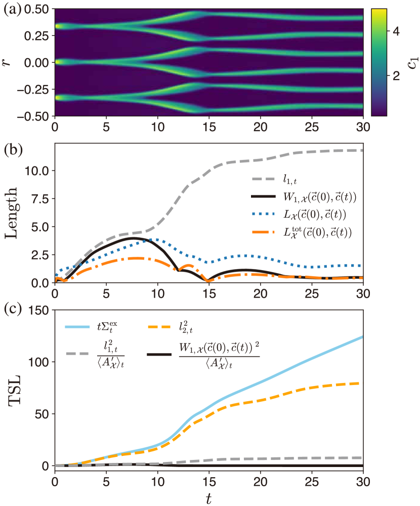
Figure 10: The lengths and the TSLs in the Brusselator model. (a) The time series of $c_{1}$ (for comparison). The figure shows the time interval $[0,30]$ of Fig. 6(a). (b) Various lengths between $\mathchoice{\kern-0.15pt\overset{\kern 0.7pt\smash{\lower 1.07639pt\hbox{\scalebox{0.45}{$\bm{\rightarrow}$}}}\kern-0.3pt}{c}}{\kern-0.15pt\overset{\kern 0.7pt\smash{\lower 1.07639pt\hbox{\scalebox{0.45}{$\bm{\rightarrow}$}}}\kern-0.3pt}{c}}{\overset{\smash{\lower 0.6458pt\hbox{\kern 0.2pt\scalebox{0.3}{$\bm{\rightarrow}$}\kern-0.8pt}}}{c}}{\overset{\smash{\lower 0.6458pt\hbox{\kern 0.2pt\scalebox{0.3}{$\bm{\rightarrow}$}\kern-0.8pt}}}{c}}(0)$ and $\mathchoice{\kern-0.15pt\overset{\kern 0.7pt\smash{\lower 1.07639pt\hbox{\scalebox{0.45}{$\bm{\rightarrow}$}}}\kern-0.3pt}{c}}{\kern-0.15pt\overset{\kern 0.7pt\smash{\lower 1.07639pt\hbox{\scalebox{0.45}{$\bm{\rightarrow}$}}}\kern-0.3pt}{c}}{\overset{\smash{\lower 0.6458pt\hbox{\kern 0.2pt\scalebox{0.3}{$\bm{\rightarrow}$}\kern-0.8pt}}}{c}}{\overset{\smash{\lower 0.6458pt\hbox{\kern 0.2pt\scalebox{0.3}{$\bm{\rightarrow}$}\kern-0.8pt}}}{c}}(t)$: $l_{1,t}$ (black line), ${W}_{1,\mathcal{X}}(\mathchoice{\kern-0.15pt\overset{\kern 0.7pt\smash{\lower 1.07639pt\hbox{\scalebox{0.45}{$\bm{\rightarrow}$}}}\kern-0.3pt}{c}}{\kern-0.15pt\overset{\kern 0.7pt\smash{\lower 1.07639pt\hbox{\scalebox{0.45}{$\bm{\rightarrow}$}}}\kern-0.3pt}{c}}{\overset{\smash{\lower 0.6458pt\hbox{\kern 0.2pt\scalebox{0.3}{$\bm{\rightarrow}$}\kern-0.8pt}}}{c}}{\overset{\smash{\lower 0.6458pt\hbox{\kern 0.2pt\scalebox{0.3}{$\bm{\rightarrow}$}\kern-0.8pt}}}{c}}(0),\mathchoice{\kern-0.15pt\overset{\kern 0.7pt\smash{\lower 1.07639pt\hbox{\scalebox{0.45}{$\bm{\rightarrow}$}}}\kern-0.3pt}{c}}{\kern-0.15pt\overset{\kern 0.7pt\smash{\lower 1.07639pt\hbox{\scalebox{0.45}{$\bm{\rightarrow}$}}}\kern-0.3pt}{c}}{\overset{\smash{\lower 0.6458pt\hbox{\kern 0.2pt\scalebox{0.3}{$\bm{\rightarrow}$}\kern-0.8pt}}}{c}}{\overset{\smash{\lower 0.6458pt\hbox{\kern 0.2pt\scalebox{0.3}{$\bm{\rightarrow}$}\kern-0.8pt}}}{c}}(t))$ (gray dashed line), ${L}_{\mathcal{X}}(\mathchoice{\kern-0.15pt\overset{\kern 0.7pt\smash{\lower 1.07639pt\hbox{\scalebox{0.45}{$\bm{\rightarrow}$}}}\kern-0.3pt}{c}}{\kern-0.15pt\overset{\kern 0.7pt\smash{\lower 1.07639pt\hbox{\scalebox{0.45}{$\bm{\rightarrow}$}}}\kern-0.3pt}{c}}{\overset{\smash{\lower 0.6458pt\hbox{\kern 0.2pt\scalebox{0.3}{$\bm{\rightarrow}$}\kern-0.8pt}}}{c}}{\overset{\smash{\lower 0.6458pt\hbox{\kern 0.2pt\scalebox{0.3}{$\bm{\rightarrow}$}\kern-0.8pt}}}{c}}(0),\mathchoice{\kern-0.15pt\overset{\kern 0.7pt\smash{\lower 1.07639pt\hbox{\scalebox{0.45}{$\bm{\rightarrow}$}}}\kern-0.3pt}{c}}{\kern-0.15pt\overset{\kern 0.7pt\smash{\lower 1.07639pt\hbox{\scalebox{0.45}{$\bm{\rightarrow}$}}}\kern-0.3pt}{c}}{\overset{\smash{\lower 0.6458pt\hbox{\kern 0.2pt\scalebox{0.3}{$\bm{\rightarrow}$}\kern-0.8pt}}}{c}}{\overset{\smash{\lower 0.6458pt\hbox{\kern 0.2pt\scalebox{0.3}{$\bm{\rightarrow}$}\kern-0.8pt}}}{c}}(t))$ (blue dotted line), and ${L}_{\mathcal{X}}^{\mathrm{tot}}(\mathchoice{\kern-0.15pt\overset{\kern 0.7pt\smash{\lower 1.07639pt\hbox{\scalebox{0.45}{$\bm{\rightarrow}$}}}\kern-0.3pt}{c}}{\kern-0.15pt\overset{\kern 0.7pt\smash{\lower 1.07639pt\hbox{\scalebox{0.45}{$\bm{\rightarrow}$}}}\kern-0.3pt}{c}}{\overset{\smash{\lower 0.6458pt\hbox{\kern 0.2pt\scalebox{0.3}{$\bm{\rightarrow}$}\kern-0.8pt}}}{c}}{\overset{\smash{\lower 0.6458pt\hbox{\kern 0.2pt\scalebox{0.3}{$\bm{\rightarrow}$}\kern-0.8pt}}}{c}}(0),\mathchoice{\kern-0.15pt\overset{\kern 0.7pt\smash{\lower 1.07639pt\hbox{\scalebox{0.45}{$\bm{\rightarrow}$}}}\kern-0.3pt}{c}}{\kern-0.15pt\overset{\kern 0.7pt\smash{\lower 1.07639pt\hbox{\scalebox{0.45}{$\bm{\rightarrow}$}}}\kern-0.3pt}{c}}{\overset{\smash{\lower 0.6458pt\hbox{\kern 0.2pt\scalebox{0.3}{$\bm{\rightarrow}$}\kern-0.8pt}}}{c}}{\overset{\smash{\lower 0.6458pt\hbox{\kern 0.2pt\scalebox{0.3}{$\bm{\rightarrow}$}\kern-0.8pt}}}{c}}(t))$ (orange dash-dotted line). There are no obvious relations between $L^{1}$-distances $({L}_{\mathcal{X}},{L}_{\mathcal{X}}^{\mathrm{tot}})$ and the 1-Wasserstein distance ${W}_{1,\mathcal{X}}$. We see the triangle inequality $l_{1,t}\geq{W}_{1,\mathcal{X}}(\mathchoice{\kern-0.15pt\overset{\kern 0.7pt\smash{\lower 1.07639pt\hbox{\scalebox{0.45}{$\bm{\rightarrow}$}}}\kern-0.3pt}{c}}{\kern-0.15pt\overset{\kern 0.7pt\smash{\lower 1.07639pt\hbox{\scalebox{0.45}{$\bm{\rightarrow}$}}}\kern-0.3pt}{c}}{\overset{\smash{\lower 0.6458pt\hbox{\kern 0.2pt\scalebox{0.3}{$\bm{\rightarrow}$}\kern-0.8pt}}}{c}}{\overset{\smash{\lower 0.6458pt\hbox{\kern 0.2pt\scalebox{0.3}{$\bm{\rightarrow}$}\kern-0.8pt}}}{c}}(0),\mathchoice{\kern-0.15pt\overset{\kern 0.7pt\smash{\lower 1.07639pt\hbox{\scalebox{0.45}{$\bm{\rightarrow}$}}}\kern-0.3pt}{c}}{\kern-0.15pt\overset{\kern 0.7pt\smash{\lower 1.07639pt\hbox{\scalebox{0.45}{$\bm{\rightarrow}$}}}\kern-0.3pt}{c}}{\overset{\smash{\lower 0.6458pt\hbox{\kern 0.2pt\scalebox{0.3}{$\bm{\rightarrow}$}\kern-0.8pt}}}{c}}{\overset{\smash{\lower 0.6458pt\hbox{\kern 0.2pt\scalebox{0.3}{$\bm{\rightarrow}$}\kern-0.8pt}}}{c}}(t))$. (c) The TSLs: $t\Sigma^{\mathrm{ex}}_{t}\geq l_{2,t}^{2}$ and $t\Sigma^{\mathrm{ex}}_{t}\geq l_{1,t}^{2}/\left\langle A^{\prime}_{\mathcal{X}}\right\rangle_{t}\geq{W}_{1,\mathcal{X}}(\mathchoice{\kern-0.15pt\overset{\kern 0.7pt\smash{\lower 1.07639pt\hbox{\scalebox{0.45}{$\bm{\rightarrow}$}}}\kern-0.3pt}{c}}{\kern-0.15pt\overset{\kern 0.7pt\smash{\lower 1.07639pt\hbox{\scalebox{0.45}{$\bm{\rightarrow}$}}}\kern-0.3pt}{c}}{\overset{\smash{\lower 0.6458pt\hbox{\kern 0.2pt\scalebox{0.3}{$\bm{\rightarrow}$}\kern-0.8pt}}}{c}}{\overset{\smash{\lower 0.6458pt\hbox{\kern 0.2pt\scalebox{0.3}{$\bm{\rightarrow}$}\kern-0.8pt}}}{c}}(0),\mathchoice{\kern-0.15pt\overset{\kern 0.7pt\smash{\lower 1.07639pt\hbox{\scalebox{0.45}{$\bm{\rightarrow}$}}}\kern-0.3pt}{c}}{\kern-0.15pt\overset{\kern 0.7pt\smash{\lower 1.07639pt\hbox{\scalebox{0.45}{$\bm{\rightarrow}$}}}\kern-0.3pt}{c}}{\overset{\smash{\lower 0.6458pt\hbox{\kern 0.2pt\scalebox{0.3}{$\bm{\rightarrow}$}\kern-0.8pt}}}{c}}{\overset{\smash{\lower 0.6458pt\hbox{\kern 0.2pt\scalebox{0.3}{$\bm{\rightarrow}$}\kern-0.8pt}}}{c}}(t))^{2}/\left\langle A^{\prime}_{\mathcal{X}}\right\rangle_{t}$. All the TSLs hold, and the TSL based on the path length with the 2-Wasserstein distance $l_{2,t}$ is relatively tight.

VI Thermodynamic Uncertainty relations for reaction-diffusion systems

We now provide another thermodynamic trade-off relation, TUR. We derive TURs for RDSs by focusing on the excess EPR. First, we obtain the TUR for general observables and interpret the TUR from the perspective of the Wasserstein geometry in Sec. VI.1. Second, we apply the general TUR to the Fourier coefficients of the concentration distribution in Sec. VI.2. This TUR for the Fourier coefficients is a generalization of the TUR for CRNs [58].

VI.1 General thermodynamic uncertainty relation for reaction-diffusion systems

Here, we derive the TUR for general observables. At first, we extend the inner products $\left\llangle\cdot,\cdot\right\rrangle$ and $\left\langle\cdot,\cdot\right\rangle$ to complex-valued functions by taking complex conjugates, indicated by bar $\overline{\phantom{a}}$, as

$$\left\llangle\mathcal{J}^{\prime},\mathcal{F}^{\prime}\right\rrangle \coloneqq\int_{V}d\bm{r}\quantity(\mathchoice{\kern-0.15pt\overset{\kern 0.7pt\smash{\lower 1.07639pt\hbox{\scalebox{0.45}{$\bm{\rightarrow}$}}}\kern-0.3pt}{\bm{J}}}{\kern-0.15pt\overset{\kern 0.7pt\smash{\lower 1.07639pt\hbox{\scalebox{0.45}{$\bm{\rightarrow}$}}}\kern-0.3pt}{\bm{J}}}{\overset{\smash{\lower 0.6458pt\hbox{\kern 0.2pt\scalebox{0.3}{$\bm{\rightarrow}$}\kern-0.8pt}}}{\bm{J}}}{\overset{\smash{\lower 0.6458pt\hbox{\kern 0.2pt\scalebox{0.3}{$\bm{\rightarrow}$}\kern-0.8pt}}}{\bm{J}}}{}^{{}^{\prime}{\dagger}}\mathchoice{\kern-0.15pt\overset{\kern 0.7pt\smash{\lower 1.07639pt\hbox{\scalebox{0.45}{$\bm{\rightarrow}$}}}\kern-0.3pt}{\bm{F}^{\prime}}}{\kern-0.15pt\overset{\kern 0.7pt\smash{\lower 1.07639pt\hbox{\scalebox{0.45}{$\bm{\rightarrow}$}}}\kern-0.3pt}{\bm{F}^{\prime}}}{\overset{\smash{\lower 0.6458pt\hbox{\kern 0.2pt\scalebox{0.3}{$\bm{\rightarrow}$}\kern-0.8pt}}}{\bm{F}^{\prime}}}{\overset{\smash{\lower 0.6458pt\hbox{\kern 0.2pt\scalebox{0.3}{$\bm{\rightarrow}$}\kern-0.8pt}}}{\bm{F}^{\prime}}}+\bm{j}^{\prime{\dagger}}\bm{f}^{\prime})$$

$$=\int_{V}d\bm{r}\left(\sum_{\alpha\in\mathcal{S}}\overline{\bm{J}^{\prime}}_{(\alpha)}\cdot\bm{F}^{\prime}_{\alpha}+\sum_{\rho\in\mathcal{R}}\overline{j^{\prime}_{\rho}}f^{\prime}_{\rho}\right),$$

for any complex-valued unified fields $\mathcal{J}^{\prime}$ and $\mathcal{F}^{\prime}$, and

$$\left\langle\mathchoice{\kern-0.15pt\overset{\kern 0.7pt\smash{\lower 1.07639pt\hbox{\scalebox{0.45}{$\bm{\rightarrow}$}}}\kern-0.3pt}{\phi}}{\kern-0.15pt\overset{\kern 0.7pt\smash{\lower 1.07639pt\hbox{\scalebox{0.45}{$\bm{\rightarrow}$}}}\kern-0.3pt}{\phi}}{\overset{\smash{\lower 0.6458pt\hbox{\kern 0.2pt\scalebox{0.3}{$\bm{\rightarrow}$}\kern-0.8pt}}}{\phi}}{\overset{\smash{\lower 0.6458pt\hbox{\kern 0.2pt\scalebox{0.3}{$\bm{\rightarrow}$}\kern-0.8pt}}}{\phi}},\mathchoice{\kern-0.15pt\overset{\kern 0.7pt\smash{\lower 1.07639pt\hbox{\scalebox{0.45}{$\bm{\rightarrow}$}}}\kern-0.3pt}{\psi}}{\kern-0.15pt\overset{\kern 0.7pt\smash{\lower 1.07639pt\hbox{\scalebox{0.45}{$\bm{\rightarrow}$}}}\kern-0.3pt}{\psi}}{\overset{\smash{\lower 0.6458pt\hbox{\kern 0.2pt\scalebox{0.3}{$\bm{\rightarrow}$}\kern-0.8pt}}}{\psi}}{\overset{\smash{\lower 0.6458pt\hbox{\kern 0.2pt\scalebox{0.3}{$\bm{\rightarrow}$}\kern-0.8pt}}}{\psi}}\right\rangle \coloneqq\int_{V}d\bm{r}\mathchoice{\kern-0.15pt\overset{\kern 0.7pt\smash{\lower 1.07639pt\hbox{\scalebox{0.45}{$\bm{\rightarrow}$}}}\kern-0.3pt}{\phi}}{\kern-0.15pt\overset{\kern 0.7pt\smash{\lower 1.07639pt\hbox{\scalebox{0.45}{$\bm{\rightarrow}$}}}\kern-0.3pt}{\phi}}{\overset{\smash{\lower 0.6458pt\hbox{\kern 0.2pt\scalebox{0.3}{$\bm{\rightarrow}$}\kern-0.8pt}}}{\phi}}{\overset{\smash{\lower 0.6458pt\hbox{\kern 0.2pt\scalebox{0.3}{$\bm{\rightarrow}$}\kern-0.8pt}}}{\phi}}{}^{{\dagger}}\mathchoice{\kern-0.15pt\overset{\kern 0.7pt\smash{\lower 1.07639pt\hbox{\scalebox{0.45}{$\bm{\rightarrow}$}}}\kern-0.3pt}{\psi}}{\kern-0.15pt\overset{\kern 0.7pt\smash{\lower 1.07639pt\hbox{\scalebox{0.45}{$\bm{\rightarrow}$}}}\kern-0.3pt}{\psi}}{\overset{\smash{\lower 0.6458pt\hbox{\kern 0.2pt\scalebox{0.3}{$\bm{\rightarrow}$}\kern-0.8pt}}}{\psi}}{\overset{\smash{\lower 0.6458pt\hbox{\kern 0.2pt\scalebox{0.3}{$\bm{\rightarrow}$}\kern-0.8pt}}}{\psi}}=\int_{V}d\bm{r}\sum_{\alpha\in\mathcal{S}}\overline{\phi_{\alpha}}\psi_{\alpha},$$

for any complex-valued vector fields $\mathchoice{\kern-0.15pt\overset{\kern 0.7pt\smash{\lower 1.07639pt\hbox{\scalebox{0.45}{$\bm{\rightarrow}$}}}\kern-0.3pt}{\phi}}{\kern-0.15pt\overset{\kern 0.7pt\smash{\lower 1.07639pt\hbox{\scalebox{0.45}{$\bm{\rightarrow}$}}}\kern-0.3pt}{\phi}}{\overset{\smash{\lower 0.6458pt\hbox{\kern 0.2pt\scalebox{0.3}{$\bm{\rightarrow}$}\kern-0.8pt}}}{\phi}}{\overset{\smash{\lower 0.6458pt\hbox{\kern 0.2pt\scalebox{0.3}{$\bm{\rightarrow}$}\kern-0.8pt}}}{\phi}}$ and $\mathchoice{\kern-0.15pt\overset{\kern 0.7pt\smash{\lower 1.07639pt\hbox{\scalebox{0.45}{$\bm{\rightarrow}$}}}\kern-0.3pt}{\psi}}{\kern-0.15pt\overset{\kern 0.7pt\smash{\lower 1.07639pt\hbox{\scalebox{0.45}{$\bm{\rightarrow}$}}}\kern-0.3pt}{\psi}}{\overset{\smash{\lower 0.6458pt\hbox{\kern 0.2pt\scalebox{0.3}{$\bm{\rightarrow}$}\kern-0.8pt}}}{\psi}}{\overset{\smash{\lower 0.6458pt\hbox{\kern 0.2pt\scalebox{0.3}{$\bm{\rightarrow}$}\kern-0.8pt}}}{\psi}}$, where ${\dagger}$ indicates conjugate transpose. We use these inner products to derive TURs for RDSs.

In the following, we use the term ”observable” to refer to complex-valued time-independent vector functions whose external parts are zero; i.e., an observable belongs to the set $\quantity{\mathchoice{\kern-0.15pt\overset{\kern 0.7pt\smash{\lower 1.07639pt\hbox{\scalebox{0.45}{$\bm{\rightarrow}$}}}\kern-0.3pt}{\varphi}}{\kern-0.15pt\overset{\kern 0.7pt\smash{\lower 1.07639pt\hbox{\scalebox{0.45}{$\bm{\rightarrow}$}}}\kern-0.3pt}{\varphi}}{\overset{\smash{\lower 0.6458pt\hbox{\kern 0.2pt\scalebox{0.3}{$\bm{\rightarrow}$}\kern-0.8pt}}}{\varphi}}{\overset{\smash{\lower 0.6458pt\hbox{\kern 0.2pt\scalebox{0.3}{$\bm{\rightarrow}$}\kern-0.8pt}}}{\varphi}}:\mathbb{R}^{d}\to\mathbb{C}^{N}\mid\forall\alpha\in\mathcal{Y},\;\varphi_{\alpha}=0}$. We impose the periodic boundary condition on $\varphi$ if we consider systems with periodic boundaries. Then, we obtain the TUR for RDSs as a generalization of Eq. (44),

$$\left|d_{t}\!\left\langle\mathchoice{\kern-0.15pt\overset{\kern 0.7pt\smash{\lower 1.07639pt\hbox{\scalebox{0.45}{$\bm{\rightarrow}$}}}\kern-0.3pt}{c}}{\kern-0.15pt\overset{\kern 0.7pt\smash{\lower 1.07639pt\hbox{\scalebox{0.45}{$\bm{\rightarrow}$}}}\kern-0.3pt}{c}}{\overset{\smash{\lower 0.6458pt\hbox{\kern 0.2pt\scalebox{0.3}{$\bm{\rightarrow}$}\kern-0.8pt}}}{c}}{\overset{\smash{\lower 0.6458pt\hbox{\kern 0.2pt\scalebox{0.3}{$\bm{\rightarrow}$}\kern-0.8pt}}}{c}},\mathchoice{\kern-0.15pt\overset{\kern 0.7pt\smash{\lower 1.07639pt\hbox{\scalebox{0.45}{$\bm{\rightarrow}$}}}\kern-0.3pt}{\varphi}}{\kern-0.15pt\overset{\kern 0.7pt\smash{\lower 1.07639pt\hbox{\scalebox{0.45}{$\bm{\rightarrow}$}}}\kern-0.3pt}{\varphi}}{\overset{\smash{\lower 0.6458pt\hbox{\kern 0.2pt\scalebox{0.3}{$\bm{\rightarrow}$}\kern-0.8pt}}}{\varphi}}{\overset{\smash{\lower 0.6458pt\hbox{\kern 0.2pt\scalebox{0.3}{$\bm{\rightarrow}$}\kern-0.8pt}}}{\varphi}}\right\rangle\right|^{2}\leq D_{\mathchoice{\kern-0.15pt\overset{\kern 0.7pt\smash{\lower 0.75346pt\hbox{\scalebox{0.45}{$\bm{\rightarrow}$}}}\kern-0.3pt}{\varphi}}{\kern-0.15pt\overset{\kern 0.7pt\smash{\lower 0.75346pt\hbox{\scalebox{0.45}{$\bm{\rightarrow}$}}}\kern-0.3pt}{\varphi}}{\overset{\smash{\lower 0.45206pt\hbox{\kern 0.2pt\scalebox{0.3}{$\bm{\rightarrow}$}\kern-0.8pt}}}{\varphi}}{\overset{\smash{\lower 0.45206pt\hbox{\kern 0.2pt\scalebox{0.3}{$\bm{\rightarrow}$}\kern-0.8pt}}}{\varphi}}}\sigma^{\mathrm{ex}},$$ (174)

where $D_{\mathchoice{\kern-0.15pt\overset{\kern 0.7pt\smash{\lower 0.75346pt\hbox{\scalebox{0.45}{$\bm{\rightarrow}$}}}\kern-0.3pt}{\varphi}}{\kern-0.15pt\overset{\kern 0.7pt\smash{\lower 0.75346pt\hbox{\scalebox{0.45}{$\bm{\rightarrow}$}}}\kern-0.3pt}{\varphi}}{\overset{\smash{\lower 0.45206pt\hbox{\kern 0.2pt\scalebox{0.3}{$\bm{\rightarrow}$}\kern-0.8pt}}}{\varphi}}{\overset{\smash{\lower 0.45206pt\hbox{\kern 0.2pt\scalebox{0.3}{$\bm{\rightarrow}$}\kern-0.8pt}}}{\varphi}}}$ quantifies the fluctuation of $\mathchoice{\kern-0.15pt\overset{\kern 0.7pt\smash{\lower 1.07639pt\hbox{\scalebox{0.45}{$\bm{\rightarrow}$}}}\kern-0.3pt}{\varphi}}{\kern-0.15pt\overset{\kern 0.7pt\smash{\lower 1.07639pt\hbox{\scalebox{0.45}{$\bm{\rightarrow}$}}}\kern-0.3pt}{\varphi}}{\overset{\smash{\lower 0.6458pt\hbox{\kern 0.2pt\scalebox{0.3}{$\bm{\rightarrow}$}\kern-0.8pt}}}{\varphi}}{\overset{\smash{\lower 0.6458pt\hbox{\kern 0.2pt\scalebox{0.3}{$\bm{\rightarrow}$}\kern-0.8pt}}}{\varphi}}$. To define $D_{\mathchoice{\kern-0.15pt\overset{\kern 0.7pt\smash{\lower 0.75346pt\hbox{\scalebox{0.45}{$\bm{\rightarrow}$}}}\kern-0.3pt}{\varphi}}{\kern-0.15pt\overset{\kern 0.7pt\smash{\lower 0.75346pt\hbox{\scalebox{0.45}{$\bm{\rightarrow}$}}}\kern-0.3pt}{\varphi}}{\overset{\smash{\lower 0.45206pt\hbox{\kern 0.2pt\scalebox{0.3}{$\bm{\rightarrow}$}\kern-0.8pt}}}{\varphi}}{\overset{\smash{\lower 0.45206pt\hbox{\kern 0.2pt\scalebox{0.3}{$\bm{\rightarrow}$}\kern-0.8pt}}}{\varphi}}}$, we introduce the scaled diffusion coefficient [58], which quantifies the fluctuation of the deterministic reaction, at $(\bm{r};t)$ as

$$\breve{D}_{\alpha\beta}(\bm{r};t) \coloneqq\sum_{\rho\in\mathcal{R}}\frac{j_{\rho}^{+}(\bm{r};t)+j_{\rho}^{-}(\bm{r};t)}{2}S_{\alpha\rho}S_{\beta\rho}$$ (175)

$$=\sum_{\rho\in\mathcal{R}}a_{\rho}(\bm{r};t)S_{\alpha\rho}S_{\beta\rho}.$$ (176)

We define $D_{\mathchoice{\kern-0.15pt\overset{\kern 0.7pt\smash{\lower 0.75346pt\hbox{\scalebox{0.45}{$\bm{\rightarrow}$}}}\kern-0.3pt}{\varphi}}{\kern-0.15pt\overset{\kern 0.7pt\smash{\lower 0.75346pt\hbox{\scalebox{0.45}{$\bm{\rightarrow}$}}}\kern-0.3pt}{\varphi}}{\overset{\smash{\lower 0.45206pt\hbox{\kern 0.2pt\scalebox{0.3}{$\bm{\rightarrow}$}\kern-0.8pt}}}{\varphi}}{\overset{\smash{\lower 0.45206pt\hbox{\kern 0.2pt\scalebox{0.3}{$\bm{\rightarrow}$}\kern-0.8pt}}}{\varphi}}}$ by using the scaled diffusion coefficient as

$$D_{\mathchoice{\kern-0.15pt\overset{\kern 0.7pt\smash{\lower 0.75346pt\hbox{\scalebox{0.45}{$\bm{\rightarrow}$}}}\kern-0.3pt}{\varphi}}{\kern-0.15pt\overset{\kern 0.7pt\smash{\lower 0.75346pt\hbox{\scalebox{0.45}{$\bm{\rightarrow}$}}}\kern-0.3pt}{\varphi}}{\overset{\smash{\lower 0.45206pt\hbox{\kern 0.2pt\scalebox{0.3}{$\bm{\rightarrow}$}\kern-0.8pt}}}{\varphi}}{\overset{\smash{\lower 0.45206pt\hbox{\kern 0.2pt\scalebox{0.3}{$\bm{\rightarrow}$}\kern-0.8pt}}}{\varphi}}}\coloneqq\int_{V}d\bm{r}\quantity[\quantity(\bm{\nabla}_{\bm{r}}\mathchoice{\kern-0.15pt\overset{\kern 0.7pt\smash{\lower 1.07639pt\hbox{\scalebox{0.45}{$\bm{\rightarrow}$}}}\kern-0.3pt}{\varphi}}{\kern-0.15pt\overset{\kern 0.7pt\smash{\lower 1.07639pt\hbox{\scalebox{0.45}{$\bm{\rightarrow}$}}}\kern-0.3pt}{\varphi}}{\overset{\smash{\lower 0.6458pt\hbox{\kern 0.2pt\scalebox{0.3}{$\bm{\rightarrow}$}\kern-0.8pt}}}{\varphi}}{\overset{\smash{\lower 0.6458pt\hbox{\kern 0.2pt\scalebox{0.3}{$\bm{\rightarrow}$}\kern-0.8pt}}}{\varphi}})^{{\dagger}}\overset{\smash{\lower 1.07639pt\hbox{\scalebox{0.7}[0.45]{$\bm{\leftrightarrow}$}}}}{\mathsf{M}}\bm{\nabla}_{\bm{r}}\mathchoice{\kern-0.15pt\overset{\kern 0.7pt\smash{\lower 1.07639pt\hbox{\scalebox{0.45}{$\bm{\rightarrow}$}}}\kern-0.3pt}{\varphi}}{\kern-0.15pt\overset{\kern 0.7pt\smash{\lower 1.07639pt\hbox{\scalebox{0.45}{$\bm{\rightarrow}$}}}\kern-0.3pt}{\varphi}}{\overset{\smash{\lower 0.6458pt\hbox{\kern 0.2pt\scalebox{0.3}{$\bm{\rightarrow}$}\kern-0.8pt}}}{\varphi}}{\overset{\smash{\lower 0.6458pt\hbox{\kern 0.2pt\scalebox{0.3}{$\bm{\rightarrow}$}\kern-0.8pt}}}{\varphi}}+\mathchoice{\kern-0.15pt\overset{\kern 0.7pt\smash{\lower 1.07639pt\hbox{\scalebox{0.45}{$\bm{\rightarrow}$}}}\kern-0.3pt}{\varphi}}{\kern-0.15pt\overset{\kern 0.7pt\smash{\lower 1.07639pt\hbox{\scalebox{0.45}{$\bm{\rightarrow}$}}}\kern-0.3pt}{\varphi}}{\overset{\smash{\lower 0.6458pt\hbox{\kern 0.2pt\scalebox{0.3}{$\bm{\rightarrow}$}\kern-0.8pt}}}{\varphi}}{\overset{\smash{\lower 0.6458pt\hbox{\kern 0.2pt\scalebox{0.3}{$\bm{\rightarrow}$}\kern-0.8pt}}}{\varphi}}^{{\dagger}}\breve{D}\mathchoice{\kern-0.15pt\overset{\kern 0.7pt\smash{\lower 1.07639pt\hbox{\scalebox{0.45}{$\bm{\rightarrow}$}}}\kern-0.3pt}{\varphi}}{\kern-0.15pt\overset{\kern 0.7pt\smash{\lower 1.07639pt\hbox{\scalebox{0.45}{$\bm{\rightarrow}$}}}\kern-0.3pt}{\varphi}}{\overset{\smash{\lower 0.6458pt\hbox{\kern 0.2pt\scalebox{0.3}{$\bm{\rightarrow}$}\kern-0.8pt}}}{\varphi}}{\overset{\smash{\lower 0.6458pt\hbox{\kern 0.2pt\scalebox{0.3}{$\bm{\rightarrow}$}\kern-0.8pt}}}{\varphi}}].$$ (177)

The first term on the right-hand side of Eq. (177) originates from the spatial inhomogeneity of $\mathchoice{\kern-0.15pt\overset{\kern 0.7pt\smash{\lower 1.07639pt\hbox{\scalebox{0.45}{$\bm{\rightarrow}$}}}\kern-0.3pt}{\varphi}}{\kern-0.15pt\overset{\kern 0.7pt\smash{\lower 1.07639pt\hbox{\scalebox{0.45}{$\bm{\rightarrow}$}}}\kern-0.3pt}{\varphi}}{\overset{\smash{\lower 0.6458pt\hbox{\kern 0.2pt\scalebox{0.3}{$\bm{\rightarrow}$}\kern-0.8pt}}}{\varphi}}{\overset{\smash{\lower 0.6458pt\hbox{\kern 0.2pt\scalebox{0.3}{$\bm{\rightarrow}$}\kern-0.8pt}}}{\varphi}}$ and the mobility of the system, and the second term originates from the fluctuation of the reactions.

We here show the derivation of the TUR [Eq. (174)]. Firstly, we can obtain an inequality between the scaled diffusion coefficient and the edgewise Onsager coefficient as

$$\breve{D}_{\alpha\beta}\geq\sum_{\rho\in\mathcal{R}}m_{\rho}S_{\alpha\rho}S_{\beta\rho}=\sum_{\rho,\rho^{\prime}\in\mathcal{R}}[\mathsf{m}]_{\rho\rho^{\prime}}S_{\alpha\rho}S_{\beta\rho^{\prime}},$$ (178)

by using the inequality in Eq. (70). This yields

$$D_{\mathchoice{\kern-0.15pt\overset{\kern 0.7pt\smash{\lower 0.75346pt\hbox{\scalebox{0.45}{$\bm{\rightarrow}$}}}\kern-0.3pt}{\varphi}}{\kern-0.15pt\overset{\kern 0.7pt\smash{\lower 0.75346pt\hbox{\scalebox{0.45}{$\bm{\rightarrow}$}}}\kern-0.3pt}{\varphi}}{\overset{\smash{\lower 0.45206pt\hbox{\kern 0.2pt\scalebox{0.3}{$\bm{\rightarrow}$}\kern-0.8pt}}}{\varphi}}{\overset{\smash{\lower 0.45206pt\hbox{\kern 0.2pt\scalebox{0.3}{$\bm{\rightarrow}$}\kern-0.8pt}}}{\varphi}}}\geq\left\llangle\nabla\mathchoice{\kern-0.15pt\overset{\kern 0.7pt\smash{\lower 1.07639pt\hbox{\scalebox{0.45}{$\bm{\rightarrow}$}}}\kern-0.3pt}{\varphi}}{\kern-0.15pt\overset{\kern 0.7pt\smash{\lower 1.07639pt\hbox{\scalebox{0.45}{$\bm{\rightarrow}$}}}\kern-0.3pt}{\varphi}}{\overset{\smash{\lower 0.6458pt\hbox{\kern 0.2pt\scalebox{0.3}{$\bm{\rightarrow}$}\kern-0.8pt}}}{\varphi}}{\overset{\smash{\lower 0.6458pt\hbox{\kern 0.2pt\scalebox{0.3}{$\bm{\rightarrow}$}\kern-0.8pt}}}{\varphi}},\nabla\mathchoice{\kern-0.15pt\overset{\kern 0.7pt\smash{\lower 1.07639pt\hbox{\scalebox{0.45}{$\bm{\rightarrow}$}}}\kern-0.3pt}{\varphi}}{\kern-0.15pt\overset{\kern 0.7pt\smash{\lower 1.07639pt\hbox{\scalebox{0.45}{$\bm{\rightarrow}$}}}\kern-0.3pt}{\varphi}}{\overset{\smash{\lower 0.6458pt\hbox{\kern 0.2pt\scalebox{0.3}{$\bm{\rightarrow}$}\kern-0.8pt}}}{\varphi}}{\overset{\smash{\lower 0.6458pt\hbox{\kern 0.2pt\scalebox{0.3}{$\bm{\rightarrow}$}\kern-0.8pt}}}{\varphi}}\right\rrangle_{\mathcal{M}}.$$ (179)

Then, we can derive the TUR as

$$\left|d_{t}\!\left\langle\mathchoice{\kern-0.15pt\overset{\kern 0.7pt\smash{\lower 1.07639pt\hbox{\scalebox{0.45}{$\bm{\rightarrow}$}}}\kern-0.3pt}{c}}{\kern-0.15pt\overset{\kern 0.7pt\smash{\lower 1.07639pt\hbox{\scalebox{0.45}{$\bm{\rightarrow}$}}}\kern-0.3pt}{c}}{\overset{\smash{\lower 0.6458pt\hbox{\kern 0.2pt\scalebox{0.3}{$\bm{\rightarrow}$}\kern-0.8pt}}}{c}}{\overset{\smash{\lower 0.6458pt\hbox{\kern 0.2pt\scalebox{0.3}{$\bm{\rightarrow}$}\kern-0.8pt}}}{c}},\mathchoice{\kern-0.15pt\overset{\kern 0.7pt\smash{\lower 1.07639pt\hbox{\scalebox{0.45}{$\bm{\rightarrow}$}}}\kern-0.3pt}{\varphi}}{\kern-0.15pt\overset{\kern 0.7pt\smash{\lower 1.07639pt\hbox{\scalebox{0.45}{$\bm{\rightarrow}$}}}\kern-0.3pt}{\varphi}}{\overset{\smash{\lower 0.6458pt\hbox{\kern 0.2pt\scalebox{0.3}{$\bm{\rightarrow}$}\kern-0.8pt}}}{\varphi}}{\overset{\smash{\lower 0.6458pt\hbox{\kern 0.2pt\scalebox{0.3}{$\bm{\rightarrow}$}\kern-0.8pt}}}{\varphi}}\right\rangle\right|^{2} =\left|\left\langle\nabla^{{\dagger}}\mathcal{M}\mathcal{F},\mathchoice{\kern-0.15pt\overset{\kern 0.7pt\smash{\lower 1.07639pt\hbox{\scalebox{0.45}{$\bm{\rightarrow}$}}}\kern-0.3pt}{\varphi}}{\kern-0.15pt\overset{\kern 0.7pt\smash{\lower 1.07639pt\hbox{\scalebox{0.45}{$\bm{\rightarrow}$}}}\kern-0.3pt}{\varphi}}{\overset{\smash{\lower 0.6458pt\hbox{\kern 0.2pt\scalebox{0.3}{$\bm{\rightarrow}$}\kern-0.8pt}}}{\varphi}}{\overset{\smash{\lower 0.6458pt\hbox{\kern 0.2pt\scalebox{0.3}{$\bm{\rightarrow}$}\kern-0.8pt}}}{\varphi}}\right\rangle\right|^{2}=\left|\left\langle\nabla^{{\dagger}}\mathcal{M}\mathcal{F}^{\ast},\mathchoice{\kern-0.15pt\overset{\kern 0.7pt\smash{\lower 1.07639pt\hbox{\scalebox{0.45}{$\bm{\rightarrow}$}}}\kern-0.3pt}{\varphi}}{\kern-0.15pt\overset{\kern 0.7pt\smash{\lower 1.07639pt\hbox{\scalebox{0.45}{$\bm{\rightarrow}$}}}\kern-0.3pt}{\varphi}}{\overset{\smash{\lower 0.6458pt\hbox{\kern 0.2pt\scalebox{0.3}{$\bm{\rightarrow}$}\kern-0.8pt}}}{\varphi}}{\overset{\smash{\lower 0.6458pt\hbox{\kern 0.2pt\scalebox{0.3}{$\bm{\rightarrow}$}\kern-0.8pt}}}{\varphi}}\right\rangle\right|^{2}$$

$$=\left|\left\llangle\mathcal{M}\mathcal{F}^{\ast},\nabla\mathchoice{\kern-0.15pt\overset{\kern 0.7pt\smash{\lower 1.07639pt\hbox{\scalebox{0.45}{$\bm{\rightarrow}$}}}\kern-0.3pt}{\varphi}}{\kern-0.15pt\overset{\kern 0.7pt\smash{\lower 1.07639pt\hbox{\scalebox{0.45}{$\bm{\rightarrow}$}}}\kern-0.3pt}{\varphi}}{\overset{\smash{\lower 0.6458pt\hbox{\kern 0.2pt\scalebox{0.3}{$\bm{\rightarrow}$}\kern-0.8pt}}}{\varphi}}{\overset{\smash{\lower 0.6458pt\hbox{\kern 0.2pt\scalebox{0.3}{$\bm{\rightarrow}$}\kern-0.8pt}}}{\varphi}}\right\rrangle\right|^{2}=\left|\left\llangle\mathcal{F}^{\ast},\nabla\mathchoice{\kern-0.15pt\overset{\kern 0.7pt\smash{\lower 1.07639pt\hbox{\scalebox{0.45}{$\bm{\rightarrow}$}}}\kern-0.3pt}{\varphi}}{\kern-0.15pt\overset{\kern 0.7pt\smash{\lower 1.07639pt\hbox{\scalebox{0.45}{$\bm{\rightarrow}$}}}\kern-0.3pt}{\varphi}}{\overset{\smash{\lower 0.6458pt\hbox{\kern 0.2pt\scalebox{0.3}{$\bm{\rightarrow}$}\kern-0.8pt}}}{\varphi}}{\overset{\smash{\lower 0.6458pt\hbox{\kern 0.2pt\scalebox{0.3}{$\bm{\rightarrow}$}\kern-0.8pt}}}{\varphi}}\right\rrangle_{\mathcal{M}}\right|^{2}$$

$$\leq\left\llangle\nabla\mathchoice{\kern-0.15pt\overset{\kern 0.7pt\smash{\lower 1.07639pt\hbox{\scalebox{0.45}{$\bm{\rightarrow}$}}}\kern-0.3pt}{\varphi}}{\kern-0.15pt\overset{\kern 0.7pt\smash{\lower 1.07639pt\hbox{\scalebox{0.45}{$\bm{\rightarrow}$}}}\kern-0.3pt}{\varphi}}{\overset{\smash{\lower 0.6458pt\hbox{\kern 0.2pt\scalebox{0.3}{$\bm{\rightarrow}$}\kern-0.8pt}}}{\varphi}}{\overset{\smash{\lower 0.6458pt\hbox{\kern 0.2pt\scalebox{0.3}{$\bm{\rightarrow}$}\kern-0.8pt}}}{\varphi}},\nabla\mathchoice{\kern-0.15pt\overset{\kern 0.7pt\smash{\lower 1.07639pt\hbox{\scalebox{0.45}{$\bm{\rightarrow}$}}}\kern-0.3pt}{\varphi}}{\kern-0.15pt\overset{\kern 0.7pt\smash{\lower 1.07639pt\hbox{\scalebox{0.45}{$\bm{\rightarrow}$}}}\kern-0.3pt}{\varphi}}{\overset{\smash{\lower 0.6458pt\hbox{\kern 0.2pt\scalebox{0.3}{$\bm{\rightarrow}$}\kern-0.8pt}}}{\varphi}}{\overset{\smash{\lower 0.6458pt\hbox{\kern 0.2pt\scalebox{0.3}{$\bm{\rightarrow}$}\kern-0.8pt}}}{\varphi}}\right\rrangle_{\mathcal{M}}\left\llangle\mathcal{F}^{\ast},\mathcal{F}^{\ast}\right\rrangle_{\mathcal{M}}$$

$$\leq D_{\mathchoice{\kern-0.15pt\overset{\kern 0.7pt\smash{\lower 0.75346pt\hbox{\scalebox{0.45}{$\bm{\rightarrow}$}}}\kern-0.3pt}{\varphi}}{\kern-0.15pt\overset{\kern 0.7pt\smash{\lower 0.75346pt\hbox{\scalebox{0.45}{$\bm{\rightarrow}$}}}\kern-0.3pt}{\varphi}}{\overset{\smash{\lower 0.45206pt\hbox{\kern 0.2pt\scalebox{0.3}{$\bm{\rightarrow}$}\kern-0.8pt}}}{\varphi}}{\overset{\smash{\lower 0.45206pt\hbox{\kern 0.2pt\scalebox{0.3}{$\bm{\rightarrow}$}\kern-0.8pt}}}{\varphi}}}\sigma^{\mathrm{ex}},$$

where we use Eq. (81) and Eq. (105) in the first line, the boundary condition for $\mathcal{F}^{\ast}$ between the first and second line, the Cauchy–Schwarz inequality for the inner product $\left\llangle\cdot,\cdot\right\rrangle_{\mathcal{M}}$ between the second and third line, and Eq. (179) in the last transformation.

We can interpret the TUR from the viewpoint of the Wasserstein geometry, as we did for the TUR for Langevin systems in Eq. (45). By rewriting Eq. (174), we obtain

$$v_{\mathchoice{\kern-0.15pt\overset{\kern 0.7pt\smash{\lower 0.75346pt\hbox{\scalebox{0.45}{$\bm{\rightarrow}$}}}\kern-0.3pt}{\varphi}}{\kern-0.15pt\overset{\kern 0.7pt\smash{\lower 0.75346pt\hbox{\scalebox{0.45}{$\bm{\rightarrow}$}}}\kern-0.3pt}{\varphi}}{\overset{\smash{\lower 0.45206pt\hbox{\kern 0.2pt\scalebox{0.3}{$\bm{\rightarrow}$}\kern-0.8pt}}}{\varphi}}{\overset{\smash{\lower 0.45206pt\hbox{\kern 0.2pt\scalebox{0.3}{$\bm{\rightarrow}$}\kern-0.8pt}}}{\varphi}}}\coloneqq\frac{|d_{t}\!\left\langle\mathchoice{\kern-0.15pt\overset{\kern 0.7pt\smash{\lower 1.07639pt\hbox{\scalebox{0.45}{$\bm{\rightarrow}$}}}\kern-0.3pt}{c}}{\kern-0.15pt\overset{\kern 0.7pt\smash{\lower 1.07639pt\hbox{\scalebox{0.45}{$\bm{\rightarrow}$}}}\kern-0.3pt}{c}}{\overset{\smash{\lower 0.6458pt\hbox{\kern 0.2pt\scalebox{0.3}{$\bm{\rightarrow}$}\kern-0.8pt}}}{c}}{\overset{\smash{\lower 0.6458pt\hbox{\kern 0.2pt\scalebox{0.3}{$\bm{\rightarrow}$}\kern-0.8pt}}}{c}},\mathchoice{\kern-0.15pt\overset{\kern 0.7pt\smash{\lower 1.07639pt\hbox{\scalebox{0.45}{$\bm{\rightarrow}$}}}\kern-0.3pt}{\varphi}}{\kern-0.15pt\overset{\kern 0.7pt\smash{\lower 1.07639pt\hbox{\scalebox{0.45}{$\bm{\rightarrow}$}}}\kern-0.3pt}{\varphi}}{\overset{\smash{\lower 0.6458pt\hbox{\kern 0.2pt\scalebox{0.3}{$\bm{\rightarrow}$}\kern-0.8pt}}}{\varphi}}{\overset{\smash{\lower 0.6458pt\hbox{\kern 0.2pt\scalebox{0.3}{$\bm{\rightarrow}$}\kern-0.8pt}}}{\varphi}}\right\rangle|}{\sqrt{D_{\mathchoice{\kern-0.15pt\overset{\kern 0.7pt\smash{\lower 0.75346pt\hbox{\scalebox{0.45}{$\bm{\rightarrow}$}}}\kern-0.3pt}{\varphi}}{\kern-0.15pt\overset{\kern 0.7pt\smash{\lower 0.75346pt\hbox{\scalebox{0.45}{$\bm{\rightarrow}$}}}\kern-0.3pt}{\varphi}}{\overset{\smash{\lower 0.45206pt\hbox{\kern 0.2pt\scalebox{0.3}{$\bm{\rightarrow}$}\kern-0.8pt}}}{\varphi}}{\overset{\smash{\lower 0.45206pt\hbox{\kern 0.2pt\scalebox{0.3}{$\bm{\rightarrow}$}\kern-0.8pt}}}{\varphi}}}}}\leq v_{2},$$ (180)

where we used $\sigma^{\rm ex}=v_{2}^{2}$. This inequality means that the speed of the observable change $v_{\mathchoice{\kern-0.15pt\overset{\kern 0.7pt\smash{\lower 0.75346pt\hbox{\scalebox{0.45}{$\bm{\rightarrow}$}}}\kern-0.3pt}{\varphi}}{\kern-0.15pt\overset{\kern 0.7pt\smash{\lower 0.75346pt\hbox{\scalebox{0.45}{$\bm{\rightarrow}$}}}\kern-0.3pt}{\varphi}}{\overset{\smash{\lower 0.45206pt\hbox{\kern 0.2pt\scalebox{0.3}{$\bm{\rightarrow}$}\kern-0.8pt}}}{\varphi}}{\overset{\smash{\lower 0.45206pt\hbox{\kern 0.2pt\scalebox{0.3}{$\bm{\rightarrow}$}\kern-0.8pt}}}{\varphi}}}$, normalized by the indicator of fluctuation $D_{\mathchoice{\kern-0.15pt\overset{\kern 0.7pt\smash{\lower 0.75346pt\hbox{\scalebox{0.45}{$\bm{\rightarrow}$}}}\kern-0.3pt}{\varphi}}{\kern-0.15pt\overset{\kern 0.7pt\smash{\lower 0.75346pt\hbox{\scalebox{0.45}{$\bm{\rightarrow}$}}}\kern-0.3pt}{\varphi}}{\overset{\smash{\lower 0.45206pt\hbox{\kern 0.2pt\scalebox{0.3}{$\bm{\rightarrow}$}\kern-0.8pt}}}{\varphi}}{\overset{\smash{\lower 0.45206pt\hbox{\kern 0.2pt\scalebox{0.3}{$\bm{\rightarrow}$}\kern-0.8pt}}}{\varphi}}}$, can always be upper bounded by the speed of the concentration distribution $v_{2}$ measured with the $2$-Wasserstein distance.

VI.2 Thermodynamic uncertainty relations for Fourier component of concentration distribution

Here, we prove a TUR for the Fourier transform of a concentration distribution by properly choosing the observable in the general TUR [Eq. (174)]. In the following part, we only consider internal species, $\alpha\in\mathcal{X}$. We define the Fourier transform of the concentration distribution as

$$\tilde{c}_{\alpha}(\bm{k};t)\coloneqq\int_{V}d\bm{r}c_{\alpha}(\bm{r};t)e^{-\mathrm{i}\bm{k}\cdot\bm{r}},$$ (181)

where we regard $c_{\alpha}(\bm{r};t)$ as zero outside of $V$. If we consider the system with the periodic boundary condition, we obtain $c_{\alpha}(\bm{r};t)=\sum_{\bm{k}}\tilde{c}_{\alpha}(\bm{k};t)e^{\mathrm{i}\bm{k}\cdot\bm{r}}/|V|$, where $|V|$ indicates the volume of $V$. In this case, the wave vector $\bm{k}$ takes discrete values depending on the details of $V$.

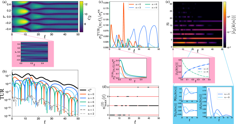
Figure 11: The TUR [Eq. (184)] in the Brusselator. (a) The time series of $c_{2}$ for comparison. In the early stage of the time evolution ($t\in[0,0.5]$), the symmetry of the pattern instantly changes from $6$-fold to $3$-fold, as shown in the pink panel. After that, the pattern goes to the steady state with $6$-fold symmetry. (b) Semilog plot of the excess EPR (black line) and the lower bounds $\sigma^{\mathrm{TUR}}_{2}(n;t)$ for various $n$. The lower bounds corresponding to multiples of $3$ ($n=0,3,6,9$) are tighter than the bounds corresponding to $n=1,\,2$. (c) The ratio of $\sigma_{2}^{\mathrm{TUR}}(n;t)$ to the excess EPR for $n=0,3,6,9$. In the early stage ($t\in[0,0.5]$), $\sigma^{\mathrm{TUR}}_{2}(3;t)$ or $\sigma^{\mathrm{TUR}}_{2}(6;t)$ provides the tightest bound as shown in the pink panel. (d) $n^{(2)}_{\mathrm{max}}(t)$ (black dots). Reflecting the symmetry of the pattern, $n^{(2)}_{\mathrm{max}}(t)$ are multiples of three for all time $t$ (red lines). Near the stationary pattern, $n^{(2)}_{\mathrm{max}}(t)=3$ for almost all $t$. (e) The time series of $|\tilde{c}_{2}(k(n))|$. We omit $|\tilde{c}_{2}(k(n))|$ for $n\geq 32$ because they are sufficiently small. The $3$-fold symmetry of the pattern lets $|\tilde{c}_{2}(k(n))|$ have large values when $n$ is a multiple of three. Since the symmetry of the pattern transitions to $6$-fold as approaching the steady state, $|\tilde{c}_{2}(k(n))|$ decays if $n$ is a multiple of three but not a multiple of six at large $t$. In contrast, the magnitude $|\tilde{c}_{2}(k(6))|$ decays while $|\tilde{c}_{2}(k(3))|$ increases in the early stage of the pattern formation (pink panel) reflecting the instant transition from the pattern with $6$-fold symmetry to the pattern with $3$-fold symmetry. The light-blue panel shows the asynchronous oscillations of the Fourier components corresponding to $n=3,\,9$ in $t\in[20,50]$. Here, we let $\mathfrak{R}[z]$ and $\mathfrak{I}[z]$ denote the real part and imaginary part of the complex number $z$, respectively. The oscillations of the two modes are not synchronized. Due to the asynchronous nature of the oscillations, the times when $\left|d_{t}\tilde{c}_{2}(k(3);t)\right|$ vanishes differ from the times when $\left|d_{t}\tilde{c}_{2}(k(9);t)\right|$ vanishes.

Fixing $\alpha\in\mathcal{X}$ and letting $\mathchoice{\kern-0.15pt\overset{\kern 0.7pt\smash{\lower 1.07639pt\hbox{\scalebox{0.45}{$\bm{\rightarrow}$}}}\kern-0.3pt}{\varphi}}{\kern-0.15pt\overset{\kern 0.7pt\smash{\lower 1.07639pt\hbox{\scalebox{0.45}{$\bm{\rightarrow}$}}}\kern-0.3pt}{\varphi}}{\overset{\smash{\lower 0.6458pt\hbox{\kern 0.2pt\scalebox{0.3}{$\bm{\rightarrow}$}\kern-0.8pt}}}{\varphi}}{\overset{\smash{\lower 0.6458pt\hbox{\kern 0.2pt\scalebox{0.3}{$\bm{\rightarrow}$}\kern-0.8pt}}}{\varphi}}$ satisfy $\quantity(\mathchoice{\kern-0.15pt\overset{\kern 0.7pt\smash{\lower 1.07639pt\hbox{\scalebox{0.45}{$\bm{\rightarrow}$}}}\kern-0.3pt}{\varphi}}{\kern-0.15pt\overset{\kern 0.7pt\smash{\lower 1.07639pt\hbox{\scalebox{0.45}{$\bm{\rightarrow}$}}}\kern-0.3pt}{\varphi}}{\overset{\smash{\lower 0.6458pt\hbox{\kern 0.2pt\scalebox{0.3}{$\bm{\rightarrow}$}\kern-0.8pt}}}{\varphi}}{\overset{\smash{\lower 0.6458pt\hbox{\kern 0.2pt\scalebox{0.3}{$\bm{\rightarrow}$}\kern-0.8pt}}}{\varphi}}(\bm{r}))_{\beta}=\delta_{\alpha\beta}e^{-\mathrm{i}\bm{k}\cdot\bm{r}}$ in Eq. (174) yields a TUR for the Fourier transform,

$$\frac{\left|d_{t}\tilde{c}_{\alpha}(\bm{k};t)\right|^{2}}{\bm{k}\cdot\mathsf{M}_{(\alpha\alpha)}^{\mathrm{tot}}(t)\bm{k}+\breve{D}^{\mathrm{tot}}_{\alpha\alpha}(t)}\leq\sigma_{t}^{\mathrm{ex}},$$ (182)

where $\mathsf{M}_{(\alpha\alpha)}^{\mathrm{tot}}(t)\coloneqq\int_{V}d\bm{r}\mathsf{M}_{(\alpha\alpha)}(\bm{r};t)$ and $\breve{D}^{\mathrm{tot}}_{\alpha\alpha}(t)=\int_{V}d\bm{r}\breve{D}_{\alpha\alpha}(\bm{r};t)$. This TUR is a generalization of the TUR for well-mixed CRNs studied in the previous work [58] because this TUR reduces to the same form as the TUR for CRNs,

$$\frac{\left|d_{t}c^{\mathrm{tot}}_{\alpha}(t)\right|^{2}}{\breve{D}^{\mathrm{tot}}_{\alpha\alpha}(t)}\leq\sigma_{t}^{\mathrm{ex}},$$ (183)

if $\bm{k}$ is $\bm{0}$. Here, we let $c^{\mathrm{tot}}_{\alpha}(t)$ denote the total concentration of $\alpha$-th species at time $t$ as $c^{\mathrm{tot}}_{\alpha}(t)\coloneqq\int_{V}d\bm{r}c_{\alpha}(\bm{r};t)$.

If the mobility tensor has the simple form in Eq. (60), we obtain a simpler form of the TUR as

$$\frac{\left|d_{t}\tilde{c}_{\alpha}(\bm{k};t)\right|^{2}}{\|\bm{k}\|^{2}D_{\alpha}c^{\mathrm{tot}}_{\alpha}(t)+\breve{D}^{\mathrm{tot}}_{\alpha\alpha}(t)}\leq\sigma_{t}^{\mathrm{ex}}.$$ (184)

The first term of the denominator in Eq. (184) monotonically increases for $\|\bm{k}\|$, while the second term is independent of $\|\bm{k}\|$. Thus, the TUR [Eq. (184)] indicates that more dissipation is needed to change the Fourier component of concentration distribution of a smaller wavenumber faster. Moreover, we can detect which mode is dominant in the time evolution by considering the tightness of the TUR [Eq. (184)] depending on wavenumber $\bm{k}$.

In the context of pattern formation, the trade-off relation Eq. (184) means that spatially global pattern formation, which is given by the mode change $|d_{t}\tilde{c}_{\alpha}(\bm{k};t)|$ corresponding to smaller wavenumber $\bm{k}$, is more dissipative rather than spatially local pattern formation, which is given by the mode change $|d_{t}\tilde{c}_{\alpha}(\bm{k}^{\prime};t)|$ corresponding to larger wavenumber $\bm{k}^{\prime}$ ($\|\bm{k}^{\prime}\|>\|\bm{k}\|$). Thus, the TUR [Eq. (184)] quantifies a required dissipation to form spatial patterns according to its spatial structure.

We can also obtain the thermodynamic trade-off relation between the change in the Fourier transform over a finite period and the dissipation as

$$\frac{\left|\tilde{c}_{\alpha}(\bm{k};\tau)-\tilde{c}_{\alpha}(\bm{k};0)\right|^{2}}{\bm{k}\cdot\langle\mathsf{M}_{(\alpha\alpha)}^{\mathrm{tot}}\rangle_{\tau}\bm{k}+\langle\breve{D}^{\mathrm{tot}}_{\alpha\alpha}\rangle_{\tau}}\leq\tau\Sigma^{\mathrm{ex}}_{\tau}.$$ (185)

Note that the initial time $0$ can be arbitrarily set. We can derive this trade-off relation by integrating the TUR in Eq. (182) over time and using the triangle inequality for time integration and the Cauchy–Schwarz inequality (see also Appendix F for details).

VI.3 Numerical examples: thermodynamic uncertainty relations

We demonstrate the TUR for the Fourier transform of a concentration distribution [Eq. (184)], using the same time series of the Brusselator as in Sec. IV.3, shown in Fig. 6. Because of the periodic boundary condition imposed on the system, we can obtain the Fourier transform of the concentration distribution as

$$\tilde{c}_{\alpha}(k(n);t)=\int_{-0.5}^{0.5}dr\,c_{\alpha}(r;t)\mathrm{e}^{-\mathrm{i}k(n)r}$$ (186)

with discrete wavenumbers $k(n)$ defined as

$$k(n)\coloneqq\frac{2n\pi}{|V_{1}|}=2n\pi,$$ (187)

with an integer $n$. Here, we use the system size $|V_{1}|=1$. To discuss the property of the TUR, we introduce the mode $n^{(\alpha)}_{\mathrm{max}}(t)$ that provides the tightest lower bound on dissipation at time $t$ in the sense of the TUR as

$$n^{(\alpha)}_{\mathrm{max}}(t)\coloneqq\operatorname*{arg\,max}_{n}\sigma^{\mathrm{TUR}}(n;t),$$ (188)

with

$$\sigma^{\mathrm{TUR}}_{\alpha}(n;t)\coloneqq\frac{\left|d_{t}\tilde{c}_{\alpha}(k(n);t)\right|^{2}}{k(n)^{2}D_{\alpha}c^{\mathrm{tot}}_{\alpha}(t)+\breve{D}^{\mathrm{tot}}_{\alpha\alpha}(t)}.$$ (189)

Here we focus on the chemical species $Z_{2}$, as indexed by $\alpha=2$ (see Appendix G for results for $Z_{1}$, corresponding to $\alpha=1$) and discuss the relations between the pattern dynamics and the lower bound of dissipation.

The lower bound in the TUR reflects the symmetry of the pattern. In this numerical example, the pattern always has a $3$-fold symmetry. Thus, the pattern changes occur only in modes corresponding to multiples of three. This leads to large $\sigma_{2}^{\mathrm{TUR}}(n;t)$ for $n$ which are multiples of three, as shown in Fig. 11 (b). After the pattern with $6$-fold symmetry is formed ($t>20$), $|\tilde{c}_{2}(k(n))|$ decays if $n$ is a multiple of three but not a multiple of six [Fig. 11(e)]. In particular, the decay of the mode $n=3$ is significant. It lets $n^{(2)}_{\mathrm{max}}(t)=3$ hold for almost all $t>20$ [Fig. 11(c) and (d)].

Rapid changes in the pattern have a significant impact on the TUR. In the early stages of the time evolution, the symmetry of the pattern instantly changes from $6$-fold to $3$-fold, as shown in the pink panel in Fig. 11(a). This change is accompanied by a rapid decay of $|\tilde{c}_{2}(k(6))|$ and a rapid increase of $|\tilde{c}_{2}(k(3))|$ [the pink panel in Fig. 11(e)]. It makes $\sigma^{\mathrm{TUR}}_{2}(n;t)$ be tighter for $n=3$ and $n=6$ than other modes, as shown in the pink panel in Fig. 11(c).

The lower bound in the TUR also reflects oscillations in the Fourier components of the pattern. The speed of change of the Fourier component $|d_{t}\tilde{c}_{2}(k(n);t)|$ intermittently goes to zero due to the oscillatory behavior of $\tilde{c}_{2}(k(n);t)$. This causes vanishing of the lower bounds $\sigma_{2}^{\mathrm{TUR}}(n;t)$, shown as sharp peaks in the semilog plot [Fig. 11(b)]. In particular, the asynchronous oscillations of $\tilde{c}_{2}(k(n);t)$ shown in the light-blue panel of Fig. 11(e) induce the temporary deviations from $n^{(2)}_{\mathrm{max}}(t)=3$ in $t\geq 20$, shown in Fig. 11(d). For example, the light-blue panel of Fig. 11(e) shows that $|d_{t}\tilde{c}_{2}(k(3);t)|$ vanishes at $t\simeq 40$, while $|d_{t}\tilde{c}_{2}(k(9);t)|$ does not. It lets $n^{(2)}_{\mathrm{max}}(t)$ deviate to nine from three at $t\simeq 39$ in Fig. 11(d).

These observations suggest that we can obtain tighter bounds of EPR by focusing on the modes according to the dynamics of the pattern. Since the denominator of $\sigma_{2}^{\mathrm{TUR}}(n;t)$ is smaller for smaller $n$, the case $n=0$ (corresponding simply to the TUR of the well-mixed CRN as Eq. (183)) gives the tightest bound if $|d_{t}\tilde{c}_{2}(k(n);t)|$ is independent of $n$. In actual pattern formation, however, the magnitude of $d_{t}\tilde{c}_{2}(k(n);t)$ is biased for each $n$, reflecting the spatiotemporal structure of the pattern. It allows $\sigma_{2}^{\mathrm{TUR}}(n;t)$ be tighter when $n$ is not zero.

VII Discussion

In this paper, we have extended the framework of geometric thermodynamics from Langevin systems, MJPs, and CRNs [55, 29, 30, 40] to RDSs: we have constructed geometric decompositions of EPR, generalized the $1$- and $2$-Wasserstein distances in optimal transport theory to RDSs, and obtained thermodynamic trade-off relations for RDSs, such as TSLs and TURs. As shown in numerical examples, our results can quantify the relations between dynamics and dissipation in pattern formation.

The geometric decompositions of EPR enable us to distinguish dissipation by its causes, e.g., we can quantify the dissipation at a wavenumber $\bm{k}$ by the wavenumber decomposition. Moreover, we can identify more detailed cause-specific dissipation by combining different geometric decompositions. For example, we have obtained $\sigma^{\mathrm{ex,wn}}_{t}(\bm{k})$, the EPR caused by the projected conservative force at the wavenumber $\bm{k}$, by combining the excess/housekeeping decomposition and the wavenumber decomposition in Sec. IV.2.

In particular, the geometric excess/housekeeping decomposition of EPR is important to relate pattern change and dissipation. This is because the decomposition separates dissipation into the part necessary to change the pattern and the part necessary to maintain the pattern. The excess EPR represents the minimum dissipation required to reproduce the original dynamics under a fixed Onsager operator $\mathcal{M}$ as shown in Eq. (112). The housekeeping EPR represents the dissipation caused by cyclic currents, which do not affect the dynamics. We remark that this decomposition is a generalization of methods developed for Langevin systems, MJPs, and CRNs [29, 30, 40], so the decomposition also generalizes the decomposition by Maes and Netočný for Langevin systems [28].

In fact, there are different options to generalize the excess/housekeeping decomposition by Maes and Netočný from Langevin systems to MJPs and CRNs. One method involves fixing another mean of the fluxes (e.g., geometric mean $\omega_{\rho}$, instead of the logarithmic mean of fluxes $m_{\rho}$) and constructing a nonlinear relation between the force and current [56]. Another method uses information geometry to study one-way fluxes, instead of the currents [42]. We may also generalize these methods to RDSs. Compared to these alternatives, the geometric excess/housekeeping decomposition proposed in this paper has several advantages: it is simple to handle because we represent the EPR as a quadratic form of the force, it allows the excess EPR to be associated with the speed of dynamics measured with the $2$-Wasserstein distance, and it is convenient for deriving thermodynamic trade-off relations.

To measure the distance between patterns in relation to thermodynamics, we have generalized the $1$- and $2$-Wasserstein distances to RDSs based on the Benamou–Brenier formula for the Wasserstein distances for continuous probability distributions. The generalized $2$-Wasserstein distance is obtained by minimizing EP while fixing the $\mathchoice{\kern-0.15pt\overset{\kern 0.7pt\smash{\lower 1.07639pt\hbox{\scalebox{0.45}{$\bm{\rightarrow}$}}}\kern-0.3pt}{c}}{\kern-0.15pt\overset{\kern 0.7pt\smash{\lower 1.07639pt\hbox{\scalebox{0.45}{$\bm{\rightarrow}$}}}\kern-0.3pt}{c}}{\overset{\smash{\lower 0.6458pt\hbox{\kern 0.2pt\scalebox{0.3}{$\bm{\rightarrow}$}\kern-0.8pt}}}{c}}{\overset{\smash{\lower 0.6458pt\hbox{\kern 0.2pt\scalebox{0.3}{$\bm{\rightarrow}$}\kern-0.8pt}}}{c}}$-dependence of $\mathcal{M}$; it is consistent with the dissipation distance defined in the study of the gradient flow structure of RDSs [59] and the $2$-Wasserstein distance for MJPs [80, 40] and CRNs [40]. From the viewpoint of the minimum EP, the speed of dynamics measured with the $2$-Wasserstein distance equals the square root of the excess EPR as shown Eq. (162). Similar to the $2$-Wasserstein distance, the generalized $1$-Wasserstein distance is consistent with the Benamou–Brenier formula of the $1$-Wasserstein distance in MJPs [41]. The $1$-Wasserstein distance is defined purely in terms of topological information (the stoichiometric matrix describing the network of reactions and the topology of the space where diffusion occurs), while the $2$-Wasserstein distance also requires kinetic information (such as the $\mathchoice{\kern-0.15pt\overset{\kern 0.7pt\smash{\lower 1.07639pt\hbox{\scalebox{0.45}{$\bm{\rightarrow}$}}}\kern-0.3pt}{c}}{\kern-0.15pt\overset{\kern 0.7pt\smash{\lower 1.07639pt\hbox{\scalebox{0.45}{$\bm{\rightarrow}$}}}\kern-0.3pt}{c}}{\overset{\smash{\lower 0.6458pt\hbox{\kern 0.2pt\scalebox{0.3}{$\bm{\rightarrow}$}\kern-0.8pt}}}{c}}{\overset{\smash{\lower 0.6458pt\hbox{\kern 0.2pt\scalebox{0.3}{$\bm{\rightarrow}$}\kern-0.8pt}}}{c}}$-dependence of $\mathcal{M}$) and it is not easy to compute. We can compare the $1$- and $2$-Wasserstein distances using the intensities of reactions and diffusive dynamics [Eq. (157)]. This shows that speed measured with the $1$-Wasserstein distance provides a lower bound on the excess EPR, as shown in Eq. (170).

Using the relations between the generalized Wasserstein distances and the excess EPR, we obtain two hierarchies of TSLs of RDSs: one based on the $2$-Wasserstein distance and the other on the $1$-Wasserstein distance. The $2$-Wasserstein distance provides the simple hierarchical TSLs [Eq. (167)], which means that the faster the speed of pattern formation, the more dissipation is required. The $1$-Wasserstein distance also provides hierarchical TSLs [Eq. (171)], which means that the faster the speed of pattern formation or the weaker the intensities of reactions and diffusive dynamics, the more dissipation is required.

In addition to TSLs, we also derived TURs for RDSs. We can obtain interesting bounds by plugging specific observables into the TUR for a general observable [Eq. (174)], according to the nature of the system. For example, we obtained a TUR for the Fourier component of $c_{\alpha}$, which means that more dissipation is required to change the Fourier components of the pattern corresponding to smaller wavenumbers. Comparing the actual dissipation with the lower bound on dissipation via the trade-off relations, we may quantify the thermodynamic efficiency of various pattern-formation processes. We also may utilize TURs to estimate the dissipation of real processes, as studied in the growing field of thermodynamic inference [84, 85].

Finally, we introduce two prospects for future research. One is the application to stochastic biological processes. Some biological processes, such as F1-ATPase [86], can be modeled as a Markov process that involves both continuous and discrete variables. The equation of motion for the probability distribution is composed of a diffusion term for the continuous variables and a Markov jump term for the discrete variables. Since Markov jump processes are formally equivalent to unimolecular CRNs, the dynamics can be regarded as a particular case of RDSs discussed in this paper. Thus, the techniques developed here could help investigate such general Markovian dynamics from the perspective of nonequilibrium thermodynamics. The other is the generalization of our results to RDSs in general spaces. While RDSs on curved surfaces [87, 88] or graphs [89, 90] have been used to study pattern formation in nature, their nonequilibrium thermodynamic properties have yet to be explored. It would be interesting to extend our results to RDSs in general spaces, for instance, by replacing the differential operator $\bm{\nabla}_{\bm{r}}$ with an appropriate counterpart for curved surfaces or graphs.

Appendix A Details of the projected force in Langevin systems

In this section, we provide the details of the conservative force $\bm{F}^{\ast}$. We derive the condition in Eq. (9) from the orthogonality [Eq. (8)] and the uniqueness of $\bm{F}^{\ast}$ by using the condition in Appendix A.1. We also derive the minimization problem in Eq. (13) and Eq. (15) in Appendix A.2. In Appendix A.3, we provide the way to obtain the condition [Eq. (9)] from the minimization problems in Eq. (13) and Eq. (15).

A.1 Sufficiency of Eq. (9) for orthogonality, and the uniqueness of its solution

Letting $\bm{F}^{\ast}$ be the gradient of a potential as $\bm{F}^{\ast}=\bm{\nabla}_{\bm{r}}\phi^{\ast}$, we can rewrite the inner product between $\bm{F}^{\ast}$ and $\bm{F}-\bm{F}^{\ast}$ as

$$\left\llangle\bm{F}^{\ast},\bm{F}-\bm{F}^{\ast}\right\rrangle_{\mathsf{M}} =\left\llangle\bm{\nabla}_{\bm{r}}\phi^{\ast},\bm{F}-\bm{\nabla}_{\bm{r}}\phi^{\ast}\right\rrangle_{\mathsf{M}}$$

$$=\int_{\mathbb{R}^{d}}d\bm{r}\bm{\nabla}_{\bm{r}}\phi^{\ast}\cdot\mathsf{M}(\bm{F}-\bm{\nabla}_{\bm{r}}\phi^{\ast})$$

$$=-\int_{\mathbb{R}^{d}}d\bm{r}\phi^{\ast}\bm{\nabla}_{\bm{r}}\cdot[\mathsf{M}(\bm{F}-\bm{\nabla}_{\bm{r}}\phi^{\ast})],$$ (190)

where we used the boundary condition for $p(\bm{r};t)$ to ignore the surface term in the third line. Then, the orthogonality in Eq. (8) reduces to

$$\int_{\mathbb{R}^{d}}d\bm{r}\phi^{\ast}\bm{\nabla}_{\bm{r}}\cdot[\mathsf{M}(\bm{F}-\bm{\nabla}_{\bm{r}}\phi^{\ast})]=0,$$ (191)

which shows that Eq. (9) is a sufficient condition of the orthogonality.

Let $\phi^{1}$ and $\phi^{2}$ be solutions of Eq. (9), and $\bm{F}^{1}$ and $\bm{F}^{2}$ the corresponding gradient forces. The norm of the difference between these forces is zero because

$$\left\llangle\bm{F}^{1}-\bm{F}^{2},\bm{F}^{1}-\bm{F}^{2}\right\rrangle_{\mathsf{M}}$$

$$=\int_{\mathbb{R}^{d}}d\bm{r}\bm{\nabla}_{\bm{r}}(\phi^{1}-\phi^{2})\cdot\mathsf{M}\bm{\nabla}_{\bm{r}}(\phi^{1}-\phi^{2})$$

$$=-\int_{\mathbb{R}^{d}}d\bm{r}(\phi^{1}-\phi^{2})\bm{\nabla}_{\bm{r}}\cdot[\mathsf{M}\{\bm{\nabla}_{\bm{r}}(\phi^{1}-\phi^{2})\}]$$

$$=\int_{\mathbb{R}^{d}}d\bm{r}(\phi^{1}-\phi^{2})\bm{\nabla}_{\bm{r}}\cdot[\mathsf{M}(\bm{F}-\bm{F})]=0$$ (192)

where we used the boundary condition for $p(\bm{r};t)$ to ignore the surface term in the third line, and Eq. (9) in the fourth line. Therefore, the two forces are identical as the norm is nondegenerate. Note that the potential satisfying Eq. (9) is not unique because $\phi^{\ast}+C$, where $C$ is a constant, is a solution of Eq. (9) when $\phi^{\ast}$ is a solution.

A.2 The derivation of minimization problems [Eqs. (13) and (15)]

The condition in Eq. (9) also leads to the orthogonality

$$\left\llangle\bm{F}^{\ast},\bm{F}^{\prime}-\bm{F}^{\ast}\right\rrangle_{\mathsf{M}}=0,$$ (193)

where $\bm{F}^{\prime}$ satisfies the condition in Eq. (13). We can check it by calculating similarly to Eq. (A.1). Using the orthogonality in Eq. (193), we obtain the inequality

$$\left\llangle\bm{F}^{\prime},\bm{F}^{\prime}\right\rrangle_{\mathsf{M}} =\left\llangle\bm{F}^{\ast},\bm{F}^{\ast}\right\rrangle_{\mathsf{M}}+\left\llangle\bm{F}^{\prime}-\bm{F}^{\ast},\bm{F}^{\prime}-\bm{F}^{\ast}\right\rrangle_{\mathsf{M}}$$

$$\geq\left\llangle\bm{F}^{\ast},\bm{F}^{\ast}\right\rrangle_{\mathsf{M}}$$ (194)

for all $\bm{F}^{\prime}$ satisfying the condition in Eq. (13). It immediately leads to the minimization problem in Eq. (13) because the equality in Eq. (A.2) is achieved if and only if $\bm{F}^{\prime}=\bm{F}^{\ast}$.

Similarly, the condition in Eq. (9) also leads to another orthogonality

$$\left\llangle\bm{F}-\bm{F}^{\ast},\bm{F}^{\ast}-\bm{F}^{\prime}\right\rrangle_{\mathsf{M}}=0,$$ (195)

for all $\bm{F}^{\prime}\in\mathrm{Im}\bm{\nabla}_{\bm{r}}$. It yields the inequality

$$\left\llangle\bm{F}-\bm{F}^{\prime},\bm{F}-\bm{F}^{\prime}\right\rrangle_{\mathsf{M}}$$

$$=\left\llangle\bm{F}-\bm{F}^{\ast},\bm{F}-\bm{F}^{\ast}\right\rrangle_{\mathsf{M}}+\left\llangle\bm{F}^{\ast}-\bm{F}^{\prime},\bm{F}^{\ast}-\bm{F}^{\prime}\right\rrangle_{\mathsf{M}}$$

$$\geq\left\llangle\bm{F}-\bm{F}^{\ast},\bm{F}-\bm{F}^{\ast}\right\rrangle_{\mathsf{M}},$$ (196)

which leads to the minimization problem in Eq. (15) because the equality in Eq. (A.2) is achieved if and only if $\bm{F}^{\prime}=\bm{F}^{\ast}$.

A.3 The derivation of the condition Eq. (9) as the Euler–Lagrange equation

We remark that the conditions Eq. (9) and $\bm{F}^{\ast}=\bm{\nabla}_{\bm{r}}\phi^{\ast}$ are conversely obtained from two variational problems Eqs. (14) and (16). By considering the action functionals

$$\mathcal{I}_{\rm hk}[\phi] \coloneqq\frac{1}{2}\left\llangle\bm{F}-\bm{\nabla}_{\bm{r}}\phi,\bm{F}-\bm{\nabla}_{\bm{r}}\phi\right\rrangle_{\mathsf{M}}=\int d\bm{r}I_{\rm hk},$$ (197)

$$\mathcal{I}_{\rm ex}[\bm{F}^{\prime},\phi] \coloneqq\frac{1}{2}\left\llangle\bm{F}^{\prime},\bm{F}^{\prime}\right\rrangle_{\mathsf{M}}+\int d\bm{r}\phi\{\bm{\nabla}_{\bm{r}}\cdot\quantity[\mathsf{M}\quantity(\bm{F}-\bm{F}^{\prime})]\}$$

$$=\int d\bm{r}I_{\rm ex}$$ (198)

with

$$I_{\rm hk} \coloneqq\frac{1}{2}(\bm{F}-\bm{\nabla}_{\bm{r}}\phi)\cdot\mathsf{M}(\bm{F}-\bm{\nabla}_{\bm{r}}\phi),$$ (199)

$$I_{\rm ex} \coloneqq\frac{1}{2}\bm{F}^{\prime}\cdot\mathsf{M}\bm{F}^{\prime}-\bm{\nabla}_{\bm{r}}\phi\cdot\mathsf{M}(\bm{F}-\bm{F}^{\prime}),$$ (200)

the two variational problems, Eqs. (14) and (16), are solved by the Euler–Lagrange equations

$$\left.\frac{\delta\mathcal{I}_{\rm hk}[\phi]}{\delta\phi}\right|_{\phi=\phi^{\ast}}=\left.\left[\frac{\partial I_{\rm hk}}{\partial\phi}-\bm{\nabla}_{\bm{r}}\cdot\frac{\partial I_{\rm hk}}{\partial(\bm{\nabla}_{\bm{r}}\phi)}\right]\right|_{\phi=\phi^{\ast}}=0,$$ (201)

$$\left.\frac{\delta\mathcal{I}_{\rm ex}[\bm{F}^{\prime},\phi]}{\delta\bm{F}^{\prime}}\right|_{\bm{F}^{\prime}=\bm{F}^{\ast},\phi=\phi^{\ast}}=\left.\frac{\partial{I}_{\rm ex}}{\partial\bm{F}^{\prime}}\right|_{\bm{F}^{\prime}=\bm{F}^{\ast},\phi=\phi^{\ast}}=\bf{0}.$$ (202)

Here, $\phi$ in Eq. (198) is the Lagrange multiplier which gives the condition in Eq. (9) from the variation $\left.\delta\mathcal{I}_{\rm ex}[\bm{F}^{\prime},\phi^{\ast}]/\delta\phi^{*}\right|_{\bm{F}^{\prime}=\bm{F}^{\ast},\phi=\phi^{\ast}}=0$. The first Euler–Lagrange equation [Eq. (201)] directly provides the condition in Eq. (9). On the other hand, the second Euler–Lagrange equation [Eq. (202)] provides $\bm{F}^{\ast}=\bm{\nabla}_{\bm{r}}\phi^{\ast}$, which leads to Eq. (9) by substituted for the constraint $\bm{\nabla}_{\bm{r}}\cdot\quantity[\mathsf{M}\quantity(\bm{F}-\bm{F}^{\prime})]=\bm{0}$.

Appendix B Details of the projected force in reaction-diffusion systems

Here, we derive the Euler–Lagrange equation in Eq. (105) from the optimization problem in Eq. (104) or Eq. (107). We also derive the uniqueness of $\mathcal{F}^{\ast}$. The derivation reduces to the case of the Langevin systems in Appendix A.3 by considering a particular situation: There are only one species and no chemical reactions.

B.1 The Euler–Lagrange equation for the projection and the uniqueness of the projected conservative force

Firstly, we derive Eq. (105) from Eq. (104). We define a functional to minimize as $\mathcal{I}_{\mathrm{hk}}[\mathchoice{\kern-0.15pt\overset{\kern 0.7pt\smash{\lower 1.07639pt\hbox{\scalebox{0.45}{$\bm{\rightarrow}$}}}\kern-0.3pt}{\phi}}{\kern-0.15pt\overset{\kern 0.7pt\smash{\lower 1.07639pt\hbox{\scalebox{0.45}{$\bm{\rightarrow}$}}}\kern-0.3pt}{\phi}}{\overset{\smash{\lower 0.6458pt\hbox{\kern 0.2pt\scalebox{0.3}{$\bm{\rightarrow}$}\kern-0.8pt}}}{\phi}}{\overset{\smash{\lower 0.6458pt\hbox{\kern 0.2pt\scalebox{0.3}{$\bm{\rightarrow}$}\kern-0.8pt}}}{\phi}}]\coloneqq\left\llangle\mathcal{F}-\nabla\mathchoice{\kern-0.15pt\overset{\kern 0.7pt\smash{\lower 1.07639pt\hbox{\scalebox{0.45}{$\bm{\rightarrow}$}}}\kern-0.3pt}{\phi}}{\kern-0.15pt\overset{\kern 0.7pt\smash{\lower 1.07639pt\hbox{\scalebox{0.45}{$\bm{\rightarrow}$}}}\kern-0.3pt}{\phi}}{\overset{\smash{\lower 0.6458pt\hbox{\kern 0.2pt\scalebox{0.3}{$\bm{\rightarrow}$}\kern-0.8pt}}}{\phi}}{\overset{\smash{\lower 0.6458pt\hbox{\kern 0.2pt\scalebox{0.3}{$\bm{\rightarrow}$}\kern-0.8pt}}}{\phi}},\mathcal{F}-\nabla\mathchoice{\kern-0.15pt\overset{\kern 0.7pt\smash{\lower 1.07639pt\hbox{\scalebox{0.45}{$\bm{\rightarrow}$}}}\kern-0.3pt}{\phi}}{\kern-0.15pt\overset{\kern 0.7pt\smash{\lower 1.07639pt\hbox{\scalebox{0.45}{$\bm{\rightarrow}$}}}\kern-0.3pt}{\phi}}{\overset{\smash{\lower 0.6458pt\hbox{\kern 0.2pt\scalebox{0.3}{$\bm{\rightarrow}$}\kern-0.8pt}}}{\phi}}{\overset{\smash{\lower 0.6458pt\hbox{\kern 0.2pt\scalebox{0.3}{$\bm{\rightarrow}$}\kern-0.8pt}}}{\phi}}\right\rrangle_{\mathcal{M}}/2=\int_{V}d\bm{r}I_{\mathrm{hk}}$ with

$$I_{\mathrm{hk}}\coloneqq \frac{1}{2}\quantity[\mathchoice{\kern-0.15pt\overset{\kern 0.7pt\smash{\lower 1.07639pt\hbox{\scalebox{0.45}{$\bm{\rightarrow}$}}}\kern-0.3pt}{\bm{F}}}{\kern-0.15pt\overset{\kern 0.7pt\smash{\lower 1.07639pt\hbox{\scalebox{0.45}{$\bm{\rightarrow}$}}}\kern-0.3pt}{\bm{F}}}{\overset{\smash{\lower 0.6458pt\hbox{\kern 0.2pt\scalebox{0.3}{$\bm{\rightarrow}$}\kern-0.8pt}}}{\bm{F}}}{\overset{\smash{\lower 0.6458pt\hbox{\kern 0.2pt\scalebox{0.3}{$\bm{\rightarrow}$}\kern-0.8pt}}}{\bm{F}}}-\bm{\nabla}_{\bm{r}}\mathchoice{\kern-0.15pt\overset{\kern 0.7pt\smash{\lower 1.07639pt\hbox{\scalebox{0.45}{$\bm{\rightarrow}$}}}\kern-0.3pt}{\phi}}{\kern-0.15pt\overset{\kern 0.7pt\smash{\lower 1.07639pt\hbox{\scalebox{0.45}{$\bm{\rightarrow}$}}}\kern-0.3pt}{\phi}}{\overset{\smash{\lower 0.6458pt\hbox{\kern 0.2pt\scalebox{0.3}{$\bm{\rightarrow}$}\kern-0.8pt}}}{\phi}}{\overset{\smash{\lower 0.6458pt\hbox{\kern 0.2pt\scalebox{0.3}{$\bm{\rightarrow}$}\kern-0.8pt}}}{\phi}}]^{\top}\overset{\smash{\lower 1.07639pt\hbox{\scalebox{0.7}[0.45]{$\bm{\leftrightarrow}$}}}}{\mathsf{M}}\quantity[\mathchoice{\kern-0.15pt\overset{\kern 0.7pt\smash{\lower 1.07639pt\hbox{\scalebox{0.45}{$\bm{\rightarrow}$}}}\kern-0.3pt}{\bm{F}}}{\kern-0.15pt\overset{\kern 0.7pt\smash{\lower 1.07639pt\hbox{\scalebox{0.45}{$\bm{\rightarrow}$}}}\kern-0.3pt}{\bm{F}}}{\overset{\smash{\lower 0.6458pt\hbox{\kern 0.2pt\scalebox{0.3}{$\bm{\rightarrow}$}\kern-0.8pt}}}{\bm{F}}}{\overset{\smash{\lower 0.6458pt\hbox{\kern 0.2pt\scalebox{0.3}{$\bm{\rightarrow}$}\kern-0.8pt}}}{\bm{F}}}-\bm{\nabla}_{\bm{r}}\mathchoice{\kern-0.15pt\overset{\kern 0.7pt\smash{\lower 1.07639pt\hbox{\scalebox{0.45}{$\bm{\rightarrow}$}}}\kern-0.3pt}{\phi}}{\kern-0.15pt\overset{\kern 0.7pt\smash{\lower 1.07639pt\hbox{\scalebox{0.45}{$\bm{\rightarrow}$}}}\kern-0.3pt}{\phi}}{\overset{\smash{\lower 0.6458pt\hbox{\kern 0.2pt\scalebox{0.3}{$\bm{\rightarrow}$}\kern-0.8pt}}}{\phi}}{\overset{\smash{\lower 0.6458pt\hbox{\kern 0.2pt\scalebox{0.3}{$\bm{\rightarrow}$}\kern-0.8pt}}}{\phi}}]$$

$$+\frac{1}{2}\quantity[\bm{f}-\nabla_{\mathsf{s}}\mathchoice{\kern-0.15pt\overset{\kern 0.7pt\smash{\lower 1.07639pt\hbox{\scalebox{0.45}{$\bm{\rightarrow}$}}}\kern-0.3pt}{\phi}}{\kern-0.15pt\overset{\kern 0.7pt\smash{\lower 1.07639pt\hbox{\scalebox{0.45}{$\bm{\rightarrow}$}}}\kern-0.3pt}{\phi}}{\overset{\smash{\lower 0.6458pt\hbox{\kern 0.2pt\scalebox{0.3}{$\bm{\rightarrow}$}\kern-0.8pt}}}{\phi}}{\overset{\smash{\lower 0.6458pt\hbox{\kern 0.2pt\scalebox{0.3}{$\bm{\rightarrow}$}\kern-0.8pt}}}{\phi}}]^{\top}\mathsf{m}\quantity[\bm{f}-\nabla_{\mathsf{s}}\mathchoice{\kern-0.15pt\overset{\kern 0.7pt\smash{\lower 1.07639pt\hbox{\scalebox{0.45}{$\bm{\rightarrow}$}}}\kern-0.3pt}{\phi}}{\kern-0.15pt\overset{\kern 0.7pt\smash{\lower 1.07639pt\hbox{\scalebox{0.45}{$\bm{\rightarrow}$}}}\kern-0.3pt}{\phi}}{\overset{\smash{\lower 0.6458pt\hbox{\kern 0.2pt\scalebox{0.3}{$\bm{\rightarrow}$}\kern-0.8pt}}}{\phi}}{\overset{\smash{\lower 0.6458pt\hbox{\kern 0.2pt\scalebox{0.3}{$\bm{\rightarrow}$}\kern-0.8pt}}}{\phi}}].$$ (203)

The functional derivative of $\mathcal{I}_{\mathrm{hk}}$ leads to the condition to be satisfied by the optimal potential $\mathchoice{\kern-0.15pt\overset{\kern 0.7pt\smash{\lower 1.07639pt\hbox{\scalebox{0.45}{$\bm{\rightarrow}$}}}\kern-0.3pt}{\phi}}{\kern-0.15pt\overset{\kern 0.7pt\smash{\lower 1.07639pt\hbox{\scalebox{0.45}{$\bm{\rightarrow}$}}}\kern-0.3pt}{\phi}}{\overset{\smash{\lower 0.6458pt\hbox{\kern 0.2pt\scalebox{0.3}{$\bm{\rightarrow}$}\kern-0.8pt}}}{\phi}}{\overset{\smash{\lower 0.6458pt\hbox{\kern 0.2pt\scalebox{0.3}{$\bm{\rightarrow}$}\kern-0.8pt}}}{\phi}}{}^{\ast}$ as

$$\left.\frac{\delta\mathcal{I}_{\mathrm{hk}}}{\delta\phi_{\alpha}}\right|_{\mathchoice{\kern-0.15pt\overset{\kern 0.7pt\smash{\lower 0.75346pt\hbox{\scalebox{0.45}{$\bm{\rightarrow}$}}}\kern-0.3pt}{\phi}}{\kern-0.15pt\overset{\kern 0.7pt\smash{\lower 0.75346pt\hbox{\scalebox{0.45}{$\bm{\rightarrow}$}}}\kern-0.3pt}{\phi}}{\overset{\smash{\lower 0.45206pt\hbox{\kern 0.2pt\scalebox{0.3}{$\bm{\rightarrow}$}\kern-0.8pt}}}{\phi}}{\overset{\smash{\lower 0.45206pt\hbox{\kern 0.2pt\scalebox{0.3}{$\bm{\rightarrow}$}\kern-0.8pt}}}{\phi}}=\mathchoice{\kern-0.15pt\overset{\kern 0.7pt\smash{\lower 0.75346pt\hbox{\scalebox{0.45}{$\bm{\rightarrow}$}}}\kern-0.3pt}{\phi}}{\kern-0.15pt\overset{\kern 0.7pt\smash{\lower 0.75346pt\hbox{\scalebox{0.45}{$\bm{\rightarrow}$}}}\kern-0.3pt}{\phi}}{\overset{\smash{\lower 0.45206pt\hbox{\kern 0.2pt\scalebox{0.3}{$\bm{\rightarrow}$}\kern-0.8pt}}}{\phi}}{\overset{\smash{\lower 0.45206pt\hbox{\kern 0.2pt\scalebox{0.3}{$\bm{\rightarrow}$}\kern-0.8pt}}}{\phi}}{}^{\ast}}=\left.\quantity(\partialderivative{I_{\mathrm{hk}}}{\phi_{\alpha}}-\bm{\nabla}_{\bm{r}}\cdot\partialderivative{I_{\mathrm{hk}}}{\quantity[\bm{\nabla}_{\bm{r}}\phi_{\alpha}]})\right|_{\mathchoice{\kern-0.15pt\overset{\kern 0.7pt\smash{\lower 0.75346pt\hbox{\scalebox{0.45}{$\bm{\rightarrow}$}}}\kern-0.3pt}{\phi}}{\kern-0.15pt\overset{\kern 0.7pt\smash{\lower 0.75346pt\hbox{\scalebox{0.45}{$\bm{\rightarrow}$}}}\kern-0.3pt}{\phi}}{\overset{\smash{\lower 0.45206pt\hbox{\kern 0.2pt\scalebox{0.3}{$\bm{\rightarrow}$}\kern-0.8pt}}}{\phi}}{\overset{\smash{\lower 0.45206pt\hbox{\kern 0.2pt\scalebox{0.3}{$\bm{\rightarrow}$}\kern-0.8pt}}}{\phi}}=\mathchoice{\kern-0.15pt\overset{\kern 0.7pt\smash{\lower 0.75346pt\hbox{\scalebox{0.45}{$\bm{\rightarrow}$}}}\kern-0.3pt}{\phi}}{\kern-0.15pt\overset{\kern 0.7pt\smash{\lower 0.75346pt\hbox{\scalebox{0.45}{$\bm{\rightarrow}$}}}\kern-0.3pt}{\phi}}{\overset{\smash{\lower 0.45206pt\hbox{\kern 0.2pt\scalebox{0.3}{$\bm{\rightarrow}$}\kern-0.8pt}}}{\phi}}{\overset{\smash{\lower 0.45206pt\hbox{\kern 0.2pt\scalebox{0.3}{$\bm{\rightarrow}$}\kern-0.8pt}}}{\phi}}{}^{\ast}}$$

$$=\quantity[-\nabla_{\mathsf{s}}^{\top}\mathsf{m}\quantity(\bm{f}-\nabla_{\mathsf{s}}\mathchoice{\kern-0.15pt\overset{\kern 0.7pt\smash{\lower 1.07639pt\hbox{\scalebox{0.45}{$\bm{\rightarrow}$}}}\kern-0.3pt}{\phi}}{\kern-0.15pt\overset{\kern 0.7pt\smash{\lower 1.07639pt\hbox{\scalebox{0.45}{$\bm{\rightarrow}$}}}\kern-0.3pt}{\phi}}{\overset{\smash{\lower 0.6458pt\hbox{\kern 0.2pt\scalebox{0.3}{$\bm{\rightarrow}$}\kern-0.8pt}}}{\phi}}{\overset{\smash{\lower 0.6458pt\hbox{\kern 0.2pt\scalebox{0.3}{$\bm{\rightarrow}$}\kern-0.8pt}}}{\phi}}{}^{\ast})+\bm{\nabla}_{\bm{r}}\cdot\quantity{\overset{\smash{\lower 1.07639pt\hbox{\scalebox{0.7}[0.45]{$\bm{\leftrightarrow}$}}}}{\mathsf{M}}\quantity(\mathchoice{\kern-0.15pt\overset{\kern 0.7pt\smash{\lower 1.07639pt\hbox{\scalebox{0.45}{$\bm{\rightarrow}$}}}\kern-0.3pt}{\bm{F}}}{\kern-0.15pt\overset{\kern 0.7pt\smash{\lower 1.07639pt\hbox{\scalebox{0.45}{$\bm{\rightarrow}$}}}\kern-0.3pt}{\bm{F}}}{\overset{\smash{\lower 0.6458pt\hbox{\kern 0.2pt\scalebox{0.3}{$\bm{\rightarrow}$}\kern-0.8pt}}}{\bm{F}}}{\overset{\smash{\lower 0.6458pt\hbox{\kern 0.2pt\scalebox{0.3}{$\bm{\rightarrow}$}\kern-0.8pt}}}{\bm{F}}}-\bm{\nabla}_{\bm{r}}\mathchoice{\kern-0.15pt\overset{\kern 0.7pt\smash{\lower 1.07639pt\hbox{\scalebox{0.45}{$\bm{\rightarrow}$}}}\kern-0.3pt}{\phi}}{\kern-0.15pt\overset{\kern 0.7pt\smash{\lower 1.07639pt\hbox{\scalebox{0.45}{$\bm{\rightarrow}$}}}\kern-0.3pt}{\phi}}{\overset{\smash{\lower 0.6458pt\hbox{\kern 0.2pt\scalebox{0.3}{$\bm{\rightarrow}$}\kern-0.8pt}}}{\phi}}{\overset{\smash{\lower 0.6458pt\hbox{\kern 0.2pt\scalebox{0.3}{$\bm{\rightarrow}$}\kern-0.8pt}}}{\phi}}{}^{\ast})}]_{\alpha}$$

$$=\quantity[-\nabla^{{\dagger}}\mathcal{M}\quantity(\mathcal{F}-\nabla\mathchoice{\kern-0.15pt\overset{\kern 0.7pt\smash{\lower 1.07639pt\hbox{\scalebox{0.45}{$\bm{\rightarrow}$}}}\kern-0.3pt}{\phi}}{\kern-0.15pt\overset{\kern 0.7pt\smash{\lower 1.07639pt\hbox{\scalebox{0.45}{$\bm{\rightarrow}$}}}\kern-0.3pt}{\phi}}{\overset{\smash{\lower 0.6458pt\hbox{\kern 0.2pt\scalebox{0.3}{$\bm{\rightarrow}$}\kern-0.8pt}}}{\phi}}{\overset{\smash{\lower 0.6458pt\hbox{\kern 0.2pt\scalebox{0.3}{$\bm{\rightarrow}$}\kern-0.8pt}}}{\phi}}{}^{\ast})]_{\alpha}=0,$$ (204)

for all $\alpha\in\mathcal{X}$, while $\phi^{\ast}_{\alpha}=0$ holds for all $\alpha\in\mathcal{Y}$. This condition [Eq. (B.1)] is nothing more than the condition indicated in Eq. (105).

Second, we show that the projected conservative force $\mathcal{F}^{\ast}$ is unique, while $\mathchoice{\kern-0.15pt\overset{\kern 0.7pt\smash{\lower 1.07639pt\hbox{\scalebox{0.45}{$\bm{\rightarrow}$}}}\kern-0.3pt}{\phi}}{\kern-0.15pt\overset{\kern 0.7pt\smash{\lower 1.07639pt\hbox{\scalebox{0.45}{$\bm{\rightarrow}$}}}\kern-0.3pt}{\phi}}{\overset{\smash{\lower 0.6458pt\hbox{\kern 0.2pt\scalebox{0.3}{$\bm{\rightarrow}$}\kern-0.8pt}}}{\phi}}{\overset{\smash{\lower 0.6458pt\hbox{\kern 0.2pt\scalebox{0.3}{$\bm{\rightarrow}$}\kern-0.8pt}}}{\phi}}{}^{\ast}$ is not. If we consider a constant vector $\mathchoice{\kern-0.15pt\overset{\kern 0.7pt\smash{\lower 1.07639pt\hbox{\scalebox{0.45}{$\bm{\rightarrow}$}}}\kern-0.3pt}{C}}{\kern-0.15pt\overset{\kern 0.7pt\smash{\lower 1.07639pt\hbox{\scalebox{0.45}{$\bm{\rightarrow}$}}}\kern-0.3pt}{C}}{\overset{\smash{\lower 0.6458pt\hbox{\kern 0.2pt\scalebox{0.3}{$\bm{\rightarrow}$}\kern-0.8pt}}}{C}}{\overset{\smash{\lower 0.6458pt\hbox{\kern 0.2pt\scalebox{0.3}{$\bm{\rightarrow}$}\kern-0.8pt}}}{C}}$ satisfying $\mathchoice{\kern-0.15pt\overset{\kern 0.7pt\smash{\lower 1.07639pt\hbox{\scalebox{0.45}{$\bm{\rightarrow}$}}}\kern-0.3pt}{C}}{\kern-0.15pt\overset{\kern 0.7pt\smash{\lower 1.07639pt\hbox{\scalebox{0.45}{$\bm{\rightarrow}$}}}\kern-0.3pt}{C}}{\overset{\smash{\lower 0.6458pt\hbox{\kern 0.2pt\scalebox{0.3}{$\bm{\rightarrow}$}\kern-0.8pt}}}{C}}{\overset{\smash{\lower 0.6458pt\hbox{\kern 0.2pt\scalebox{0.3}{$\bm{\rightarrow}$}\kern-0.8pt}}}{C}}_{\mathcal{Y}}=\mathchoice{\overset{\smash{\lower 1.07639pt\hbox{\scalebox{0.45}{$\bm{\rightarrow}$}}}}{0}}{\overset{\smash{\lower 1.07639pt\hbox{\scalebox{0.45}{$\bm{\rightarrow}$}}}}{0}}{\overset{\smash{\lower 0.6458pt\hbox{\scalebox{0.3}{$\bm{\rightarrow}$}}}}{0}}{\overset{\smash{\lower 0.6458pt\hbox{\scalebox{0.3}{$\bm{\rightarrow}$}}}}{0}}_{\mathcal{Y}}$, whose gradient $\nabla\mathchoice{\kern-0.15pt\overset{\kern 0.7pt\smash{\lower 1.07639pt\hbox{\scalebox{0.45}{$\bm{\rightarrow}$}}}\kern-0.3pt}{C}}{\kern-0.15pt\overset{\kern 0.7pt\smash{\lower 1.07639pt\hbox{\scalebox{0.45}{$\bm{\rightarrow}$}}}\kern-0.3pt}{C}}{\overset{\smash{\lower 0.6458pt\hbox{\kern 0.2pt\scalebox{0.3}{$\bm{\rightarrow}$}\kern-0.8pt}}}{C}}{\overset{\smash{\lower 0.6458pt\hbox{\kern 0.2pt\scalebox{0.3}{$\bm{\rightarrow}$}\kern-0.8pt}}}{C}}$ is a zero vector, $\mathchoice{\kern-0.15pt\overset{\kern 0.7pt\smash{\lower 1.07639pt\hbox{\scalebox{0.45}{$\bm{\rightarrow}$}}}\kern-0.3pt}{\phi}}{\kern-0.15pt\overset{\kern 0.7pt\smash{\lower 1.07639pt\hbox{\scalebox{0.45}{$\bm{\rightarrow}$}}}\kern-0.3pt}{\phi}}{\overset{\smash{\lower 0.6458pt\hbox{\kern 0.2pt\scalebox{0.3}{$\bm{\rightarrow}$}\kern-0.8pt}}}{\phi}}{\overset{\smash{\lower 0.6458pt\hbox{\kern 0.2pt\scalebox{0.3}{$\bm{\rightarrow}$}\kern-0.8pt}}}{\phi}}{}^{\ast}+\mathchoice{\kern-0.15pt\overset{\kern 0.7pt\smash{\lower 1.07639pt\hbox{\scalebox{0.45}{$\bm{\rightarrow}$}}}\kern-0.3pt}{C}}{\kern-0.15pt\overset{\kern 0.7pt\smash{\lower 1.07639pt\hbox{\scalebox{0.45}{$\bm{\rightarrow}$}}}\kern-0.3pt}{C}}{\overset{\smash{\lower 0.6458pt\hbox{\kern 0.2pt\scalebox{0.3}{$\bm{\rightarrow}$}\kern-0.8pt}}}{C}}{\overset{\smash{\lower 0.6458pt\hbox{\kern 0.2pt\scalebox{0.3}{$\bm{\rightarrow}$}\kern-0.8pt}}}{C}}$ can also be a solution of the minimization problem in Eq. (104) and thus $\mathchoice{\kern-0.15pt\overset{\kern 0.7pt\smash{\lower 1.07639pt\hbox{\scalebox{0.45}{$\bm{\rightarrow}$}}}\kern-0.3pt}{\phi}}{\kern-0.15pt\overset{\kern 0.7pt\smash{\lower 1.07639pt\hbox{\scalebox{0.45}{$\bm{\rightarrow}$}}}\kern-0.3pt}{\phi}}{\overset{\smash{\lower 0.6458pt\hbox{\kern 0.2pt\scalebox{0.3}{$\bm{\rightarrow}$}\kern-0.8pt}}}{\phi}}{\overset{\smash{\lower 0.6458pt\hbox{\kern 0.2pt\scalebox{0.3}{$\bm{\rightarrow}$}\kern-0.8pt}}}{\phi}}{}^{\ast}$ is not unique. Supposing Eq. (105) has two solutions, $\mathchoice{\kern-0.15pt\overset{\kern 0.7pt\smash{\lower 1.07639pt\hbox{\scalebox{0.45}{$\bm{\rightarrow}$}}}\kern-0.3pt}{\phi}}{\kern-0.15pt\overset{\kern 0.7pt\smash{\lower 1.07639pt\hbox{\scalebox{0.45}{$\bm{\rightarrow}$}}}\kern-0.3pt}{\phi}}{\overset{\smash{\lower 0.6458pt\hbox{\kern 0.2pt\scalebox{0.3}{$\bm{\rightarrow}$}\kern-0.8pt}}}{\phi}}{\overset{\smash{\lower 0.6458pt\hbox{\kern 0.2pt\scalebox{0.3}{$\bm{\rightarrow}$}\kern-0.8pt}}}{\phi}}{}^{1}$ and $\mathchoice{\kern-0.15pt\overset{\kern 0.7pt\smash{\lower 1.07639pt\hbox{\scalebox{0.45}{$\bm{\rightarrow}$}}}\kern-0.3pt}{\phi}}{\kern-0.15pt\overset{\kern 0.7pt\smash{\lower 1.07639pt\hbox{\scalebox{0.45}{$\bm{\rightarrow}$}}}\kern-0.3pt}{\phi}}{\overset{\smash{\lower 0.6458pt\hbox{\kern 0.2pt\scalebox{0.3}{$\bm{\rightarrow}$}\kern-0.8pt}}}{\phi}}{\overset{\smash{\lower 0.6458pt\hbox{\kern 0.2pt\scalebox{0.3}{$\bm{\rightarrow}$}\kern-0.8pt}}}{\phi}}{}^{2}$, which satisfy $\mathchoice{\kern-0.15pt\overset{\kern 0.7pt\smash{\lower 1.07639pt\hbox{\scalebox{0.45}{$\bm{\rightarrow}$}}}\kern-0.3pt}{\phi}}{\kern-0.15pt\overset{\kern 0.7pt\smash{\lower 1.07639pt\hbox{\scalebox{0.45}{$\bm{\rightarrow}$}}}\kern-0.3pt}{\phi}}{\overset{\smash{\lower 0.6458pt\hbox{\kern 0.2pt\scalebox{0.3}{$\bm{\rightarrow}$}\kern-0.8pt}}}{\phi}}{\overset{\smash{\lower 0.6458pt\hbox{\kern 0.2pt\scalebox{0.3}{$\bm{\rightarrow}$}\kern-0.8pt}}}{\phi}}{}^{1}_{\mathcal{Y}}=\mathchoice{\kern-0.15pt\overset{\kern 0.7pt\smash{\lower 1.07639pt\hbox{\scalebox{0.45}{$\bm{\rightarrow}$}}}\kern-0.3pt}{\phi}}{\kern-0.15pt\overset{\kern 0.7pt\smash{\lower 1.07639pt\hbox{\scalebox{0.45}{$\bm{\rightarrow}$}}}\kern-0.3pt}{\phi}}{\overset{\smash{\lower 0.6458pt\hbox{\kern 0.2pt\scalebox{0.3}{$\bm{\rightarrow}$}\kern-0.8pt}}}{\phi}}{\overset{\smash{\lower 0.6458pt\hbox{\kern 0.2pt\scalebox{0.3}{$\bm{\rightarrow}$}\kern-0.8pt}}}{\phi}}{}^{2}_{\mathcal{Y}}=\mathchoice{\overset{\smash{\lower 1.07639pt\hbox{\scalebox{0.45}{$\bm{\rightarrow}$}}}}{0}}{\overset{\smash{\lower 1.07639pt\hbox{\scalebox{0.45}{$\bm{\rightarrow}$}}}}{0}}{\overset{\smash{\lower 0.6458pt\hbox{\scalebox{0.3}{$\bm{\rightarrow}$}}}}{0}}{\overset{\smash{\lower 0.6458pt\hbox{\scalebox{0.3}{$\bm{\rightarrow}$}}}}{0}}_{\mathcal{Y}}$, under the boundary condition, we obtain

$$\left\llangle\mathcal{F}^{1}-\mathcal{F}^{2},\mathcal{F}^{1}-\mathcal{F}^{2}\right\rrangle_{\mathcal{M}} =\left\llangle\mathcal{M}\nabla(\mathchoice{\kern-0.15pt\overset{\kern 0.7pt\smash{\lower 1.07639pt\hbox{\scalebox{0.45}{$\bm{\rightarrow}$}}}\kern-0.3pt}{\phi}}{\kern-0.15pt\overset{\kern 0.7pt\smash{\lower 1.07639pt\hbox{\scalebox{0.45}{$\bm{\rightarrow}$}}}\kern-0.3pt}{\phi}}{\overset{\smash{\lower 0.6458pt\hbox{\kern 0.2pt\scalebox{0.3}{$\bm{\rightarrow}$}\kern-0.8pt}}}{\phi}}{\overset{\smash{\lower 0.6458pt\hbox{\kern 0.2pt\scalebox{0.3}{$\bm{\rightarrow}$}\kern-0.8pt}}}{\phi}}{}^{1}-\mathchoice{\kern-0.15pt\overset{\kern 0.7pt\smash{\lower 1.07639pt\hbox{\scalebox{0.45}{$\bm{\rightarrow}$}}}\kern-0.3pt}{\phi}}{\kern-0.15pt\overset{\kern 0.7pt\smash{\lower 1.07639pt\hbox{\scalebox{0.45}{$\bm{\rightarrow}$}}}\kern-0.3pt}{\phi}}{\overset{\smash{\lower 0.6458pt\hbox{\kern 0.2pt\scalebox{0.3}{$\bm{\rightarrow}$}\kern-0.8pt}}}{\phi}}{\overset{\smash{\lower 0.6458pt\hbox{\kern 0.2pt\scalebox{0.3}{$\bm{\rightarrow}$}\kern-0.8pt}}}{\phi}}{}^{2}),\nabla(\mathchoice{\kern-0.15pt\overset{\kern 0.7pt\smash{\lower 1.07639pt\hbox{\scalebox{0.45}{$\bm{\rightarrow}$}}}\kern-0.3pt}{\phi}}{\kern-0.15pt\overset{\kern 0.7pt\smash{\lower 1.07639pt\hbox{\scalebox{0.45}{$\bm{\rightarrow}$}}}\kern-0.3pt}{\phi}}{\overset{\smash{\lower 0.6458pt\hbox{\kern 0.2pt\scalebox{0.3}{$\bm{\rightarrow}$}\kern-0.8pt}}}{\phi}}{\overset{\smash{\lower 0.6458pt\hbox{\kern 0.2pt\scalebox{0.3}{$\bm{\rightarrow}$}\kern-0.8pt}}}{\phi}}{}^{1}-\mathchoice{\kern-0.15pt\overset{\kern 0.7pt\smash{\lower 1.07639pt\hbox{\scalebox{0.45}{$\bm{\rightarrow}$}}}\kern-0.3pt}{\phi}}{\kern-0.15pt\overset{\kern 0.7pt\smash{\lower 1.07639pt\hbox{\scalebox{0.45}{$\bm{\rightarrow}$}}}\kern-0.3pt}{\phi}}{\overset{\smash{\lower 0.6458pt\hbox{\kern 0.2pt\scalebox{0.3}{$\bm{\rightarrow}$}\kern-0.8pt}}}{\phi}}{\overset{\smash{\lower 0.6458pt\hbox{\kern 0.2pt\scalebox{0.3}{$\bm{\rightarrow}$}\kern-0.8pt}}}{\phi}}{}^{2})\right\rrangle$$

$$=\left\langle\nabla^{{\dagger}}\mathcal{M}\nabla(\mathchoice{\kern-0.15pt\overset{\kern 0.7pt\smash{\lower 1.07639pt\hbox{\scalebox{0.45}{$\bm{\rightarrow}$}}}\kern-0.3pt}{\phi}}{\kern-0.15pt\overset{\kern 0.7pt\smash{\lower 1.07639pt\hbox{\scalebox{0.45}{$\bm{\rightarrow}$}}}\kern-0.3pt}{\phi}}{\overset{\smash{\lower 0.6458pt\hbox{\kern 0.2pt\scalebox{0.3}{$\bm{\rightarrow}$}\kern-0.8pt}}}{\phi}}{\overset{\smash{\lower 0.6458pt\hbox{\kern 0.2pt\scalebox{0.3}{$\bm{\rightarrow}$}\kern-0.8pt}}}{\phi}}{}^{1}-\mathchoice{\kern-0.15pt\overset{\kern 0.7pt\smash{\lower 1.07639pt\hbox{\scalebox{0.45}{$\bm{\rightarrow}$}}}\kern-0.3pt}{\phi}}{\kern-0.15pt\overset{\kern 0.7pt\smash{\lower 1.07639pt\hbox{\scalebox{0.45}{$\bm{\rightarrow}$}}}\kern-0.3pt}{\phi}}{\overset{\smash{\lower 0.6458pt\hbox{\kern 0.2pt\scalebox{0.3}{$\bm{\rightarrow}$}\kern-0.8pt}}}{\phi}}{\overset{\smash{\lower 0.6458pt\hbox{\kern 0.2pt\scalebox{0.3}{$\bm{\rightarrow}$}\kern-0.8pt}}}{\phi}}{}^{2}),\mathchoice{\kern-0.15pt\overset{\kern 0.7pt\smash{\lower 1.07639pt\hbox{\scalebox{0.45}{$\bm{\rightarrow}$}}}\kern-0.3pt}{\phi}}{\kern-0.15pt\overset{\kern 0.7pt\smash{\lower 1.07639pt\hbox{\scalebox{0.45}{$\bm{\rightarrow}$}}}\kern-0.3pt}{\phi}}{\overset{\smash{\lower 0.6458pt\hbox{\kern 0.2pt\scalebox{0.3}{$\bm{\rightarrow}$}\kern-0.8pt}}}{\phi}}{\overset{\smash{\lower 0.6458pt\hbox{\kern 0.2pt\scalebox{0.3}{$\bm{\rightarrow}$}\kern-0.8pt}}}{\phi}}{}^{1}-\mathchoice{\kern-0.15pt\overset{\kern 0.7pt\smash{\lower 1.07639pt\hbox{\scalebox{0.45}{$\bm{\rightarrow}$}}}\kern-0.3pt}{\phi}}{\kern-0.15pt\overset{\kern 0.7pt\smash{\lower 1.07639pt\hbox{\scalebox{0.45}{$\bm{\rightarrow}$}}}\kern-0.3pt}{\phi}}{\overset{\smash{\lower 0.6458pt\hbox{\kern 0.2pt\scalebox{0.3}{$\bm{\rightarrow}$}\kern-0.8pt}}}{\phi}}{\overset{\smash{\lower 0.6458pt\hbox{\kern 0.2pt\scalebox{0.3}{$\bm{\rightarrow}$}\kern-0.8pt}}}{\phi}}{}^{2}\right\rangle$$

$$=\left\langle\nabla^{{\dagger}}\mathcal{M}\quantity(\mathcal{F}-\mathcal{F}),\mathchoice{\kern-0.15pt\overset{\kern 0.7pt\smash{\lower 1.07639pt\hbox{\scalebox{0.45}{$\bm{\rightarrow}$}}}\kern-0.3pt}{\phi}}{\kern-0.15pt\overset{\kern 0.7pt\smash{\lower 1.07639pt\hbox{\scalebox{0.45}{$\bm{\rightarrow}$}}}\kern-0.3pt}{\phi}}{\overset{\smash{\lower 0.6458pt\hbox{\kern 0.2pt\scalebox{0.3}{$\bm{\rightarrow}$}\kern-0.8pt}}}{\phi}}{\overset{\smash{\lower 0.6458pt\hbox{\kern 0.2pt\scalebox{0.3}{$\bm{\rightarrow}$}\kern-0.8pt}}}{\phi}}{}^{1}-\mathchoice{\kern-0.15pt\overset{\kern 0.7pt\smash{\lower 1.07639pt\hbox{\scalebox{0.45}{$\bm{\rightarrow}$}}}\kern-0.3pt}{\phi}}{\kern-0.15pt\overset{\kern 0.7pt\smash{\lower 1.07639pt\hbox{\scalebox{0.45}{$\bm{\rightarrow}$}}}\kern-0.3pt}{\phi}}{\overset{\smash{\lower 0.6458pt\hbox{\kern 0.2pt\scalebox{0.3}{$\bm{\rightarrow}$}\kern-0.8pt}}}{\phi}}{\overset{\smash{\lower 0.6458pt\hbox{\kern 0.2pt\scalebox{0.3}{$\bm{\rightarrow}$}\kern-0.8pt}}}{\phi}}{}^{2}\right\rangle$$

$$=0,$$ (205)

where we define $\mathcal{F}^{i}\coloneqq\nabla\mathchoice{\kern-0.15pt\overset{\kern 0.7pt\smash{\lower 1.07639pt\hbox{\scalebox{0.45}{$\bm{\rightarrow}$}}}\kern-0.3pt}{\phi}}{\kern-0.15pt\overset{\kern 0.7pt\smash{\lower 1.07639pt\hbox{\scalebox{0.45}{$\bm{\rightarrow}$}}}\kern-0.3pt}{\phi}}{\overset{\smash{\lower 0.6458pt\hbox{\kern 0.2pt\scalebox{0.3}{$\bm{\rightarrow}$}\kern-0.8pt}}}{\phi}}{\overset{\smash{\lower 0.6458pt\hbox{\kern 0.2pt\scalebox{0.3}{$\bm{\rightarrow}$}\kern-0.8pt}}}{\phi}}{}^{i}$ for $i=1,2$. The second transformation in Eq. (B.1) is allowed because we are imposing the appropriate boundary condition, and the third line follows from the Euler–Lagrange equation (105). We also use the condition, $\phi^{1}_{\alpha}-\phi^{2}_{\alpha}=0$ for all $\alpha\in\mathcal{Y}$, in these transformations. Therefore, the positive-definiteness of $\mathcal{M}$ shows $\mathcal{F}^{1}=\mathcal{F}^{2}$, i.e., the uniqueness of the projected potential force.

B.2 The Euler–Lagrange equation for the minimum dissipation

We derive the condition [Eq. (105)] from the minimization problem in Eq. (107). To solve this minimization problem with constraints, we execute the method of Lagrange multiplier with the multiplier $\mathchoice{\kern-0.15pt\overset{\kern 0.7pt\smash{\lower 1.07639pt\hbox{\scalebox{0.45}{$\bm{\rightarrow}$}}}\kern-0.3pt}{\phi}}{\kern-0.15pt\overset{\kern 0.7pt\smash{\lower 1.07639pt\hbox{\scalebox{0.45}{$\bm{\rightarrow}$}}}\kern-0.3pt}{\phi}}{\overset{\smash{\lower 0.6458pt\hbox{\kern 0.2pt\scalebox{0.3}{$\bm{\rightarrow}$}\kern-0.8pt}}}{\phi}}{\overset{\smash{\lower 0.6458pt\hbox{\kern 0.2pt\scalebox{0.3}{$\bm{\rightarrow}$}\kern-0.8pt}}}{\phi}}$, whose external part is the zero vector as $\mathchoice{\kern-0.15pt\overset{\kern 0.7pt\smash{\lower 1.07639pt\hbox{\scalebox{0.45}{$\bm{\rightarrow}$}}}\kern-0.3pt}{\phi}}{\kern-0.15pt\overset{\kern 0.7pt\smash{\lower 1.07639pt\hbox{\scalebox{0.45}{$\bm{\rightarrow}$}}}\kern-0.3pt}{\phi}}{\overset{\smash{\lower 0.6458pt\hbox{\kern 0.2pt\scalebox{0.3}{$\bm{\rightarrow}$}\kern-0.8pt}}}{\phi}}{\overset{\smash{\lower 0.6458pt\hbox{\kern 0.2pt\scalebox{0.3}{$\bm{\rightarrow}$}\kern-0.8pt}}}{\phi}}_{\mathcal{Y}}=\mathchoice{\overset{\smash{\lower 1.07639pt\hbox{\scalebox{0.45}{$\bm{\rightarrow}$}}}}{0}}{\overset{\smash{\lower 1.07639pt\hbox{\scalebox{0.45}{$\bm{\rightarrow}$}}}}{0}}{\overset{\smash{\lower 0.6458pt\hbox{\scalebox{0.3}{$\bm{\rightarrow}$}}}}{0}}{\overset{\smash{\lower 0.6458pt\hbox{\scalebox{0.3}{$\bm{\rightarrow}$}}}}{0}}_{\mathcal{Y}}$. Then, the functional to optimize is

$$\mathcal{I}_{\mathrm{ex}}[\mathcal{F}^{\prime},\mathchoice{\kern-0.15pt\overset{\kern 0.7pt\smash{\lower 1.07639pt\hbox{\scalebox{0.45}{$\bm{\rightarrow}$}}}\kern-0.3pt}{\phi}}{\kern-0.15pt\overset{\kern 0.7pt\smash{\lower 1.07639pt\hbox{\scalebox{0.45}{$\bm{\rightarrow}$}}}\kern-0.3pt}{\phi}}{\overset{\smash{\lower 0.6458pt\hbox{\kern 0.2pt\scalebox{0.3}{$\bm{\rightarrow}$}\kern-0.8pt}}}{\phi}}{\overset{\smash{\lower 0.6458pt\hbox{\kern 0.2pt\scalebox{0.3}{$\bm{\rightarrow}$}\kern-0.8pt}}}{\phi}}] \coloneqq\frac{1}{2}\left\llangle\mathcal{F}^{\prime},\mathcal{F}^{\prime}\right\rrangle_{\mathcal{M}}+\left\langle\mathchoice{\kern-0.15pt\overset{\kern 0.7pt\smash{\lower 1.07639pt\hbox{\scalebox{0.45}{$\bm{\rightarrow}$}}}\kern-0.3pt}{\phi}}{\kern-0.15pt\overset{\kern 0.7pt\smash{\lower 1.07639pt\hbox{\scalebox{0.45}{$\bm{\rightarrow}$}}}\kern-0.3pt}{\phi}}{\overset{\smash{\lower 0.6458pt\hbox{\kern 0.2pt\scalebox{0.3}{$\bm{\rightarrow}$}\kern-0.8pt}}}{\phi}}{\overset{\smash{\lower 0.6458pt\hbox{\kern 0.2pt\scalebox{0.3}{$\bm{\rightarrow}$}\kern-0.8pt}}}{\phi}},\nabla^{{\dagger}}\mathcal{M}\quantity(\mathcal{F}-\mathcal{F}^{\prime})\right\rangle$$

$$=\frac{1}{2}\left\llangle\mathcal{F}^{\prime},\mathcal{F}^{\prime}\right\rrangle_{\mathcal{M}}+\left\llangle\nabla\mathchoice{\kern-0.15pt\overset{\kern 0.7pt\smash{\lower 1.07639pt\hbox{\scalebox{0.45}{$\bm{\rightarrow}$}}}\kern-0.3pt}{\phi}}{\kern-0.15pt\overset{\kern 0.7pt\smash{\lower 1.07639pt\hbox{\scalebox{0.45}{$\bm{\rightarrow}$}}}\kern-0.3pt}{\phi}}{\overset{\smash{\lower 0.6458pt\hbox{\kern 0.2pt\scalebox{0.3}{$\bm{\rightarrow}$}\kern-0.8pt}}}{\phi}}{\overset{\smash{\lower 0.6458pt\hbox{\kern 0.2pt\scalebox{0.3}{$\bm{\rightarrow}$}\kern-0.8pt}}}{\phi}},\mathcal{F}-\mathcal{F}^{\prime}\right\rrangle_{\mathcal{M}}.$$ (206)

We obtain the conditions to be satisfied by the optimizer $\mathcal{F}^{\ast}$ and $\mathchoice{\kern-0.15pt\overset{\kern 0.7pt\smash{\lower 1.07639pt\hbox{\scalebox{0.45}{$\bm{\rightarrow}$}}}\kern-0.3pt}{\phi}}{\kern-0.15pt\overset{\kern 0.7pt\smash{\lower 1.07639pt\hbox{\scalebox{0.45}{$\bm{\rightarrow}$}}}\kern-0.3pt}{\phi}}{\overset{\smash{\lower 0.6458pt\hbox{\kern 0.2pt\scalebox{0.3}{$\bm{\rightarrow}$}\kern-0.8pt}}}{\phi}}{\overset{\smash{\lower 0.6458pt\hbox{\kern 0.2pt\scalebox{0.3}{$\bm{\rightarrow}$}\kern-0.8pt}}}{\phi}}{}^{\ast}$ by taking the functional derivative of $\mathcal{I}_{\mathrm{ex}}[\mathcal{F}^{\prime},\mathchoice{\kern-0.15pt\overset{\kern 0.7pt\smash{\lower 1.07639pt\hbox{\scalebox{0.45}{$\bm{\rightarrow}$}}}\kern-0.3pt}{\phi}}{\kern-0.15pt\overset{\kern 0.7pt\smash{\lower 1.07639pt\hbox{\scalebox{0.45}{$\bm{\rightarrow}$}}}\kern-0.3pt}{\phi}}{\overset{\smash{\lower 0.6458pt\hbox{\kern 0.2pt\scalebox{0.3}{$\bm{\rightarrow}$}\kern-0.8pt}}}{\phi}}{\overset{\smash{\lower 0.6458pt\hbox{\kern 0.2pt\scalebox{0.3}{$\bm{\rightarrow}$}\kern-0.8pt}}}{\phi}}]$ as

$$\left.\frac{\delta\mathcal{I}_{\mathrm{ex}}[\mathcal{F}^{\prime},\mathchoice{\kern-0.15pt\overset{\kern 0.7pt\smash{\lower 1.07639pt\hbox{\scalebox{0.45}{$\bm{\rightarrow}$}}}\kern-0.3pt}{\phi}}{\kern-0.15pt\overset{\kern 0.7pt\smash{\lower 1.07639pt\hbox{\scalebox{0.45}{$\bm{\rightarrow}$}}}\kern-0.3pt}{\phi}}{\overset{\smash{\lower 0.6458pt\hbox{\kern 0.2pt\scalebox{0.3}{$\bm{\rightarrow}$}\kern-0.8pt}}}{\phi}}{\overset{\smash{\lower 0.6458pt\hbox{\kern 0.2pt\scalebox{0.3}{$\bm{\rightarrow}$}\kern-0.8pt}}}{\phi}}]}{\delta\bm{F}^{\prime}_{(\alpha)}}\right|_{\mathchoice{\kern-0.15pt\overset{\kern 0.7pt\smash{\lower 0.75346pt\hbox{\scalebox{0.45}{$\bm{\rightarrow}$}}}\kern-0.3pt}{\phi}}{\kern-0.15pt\overset{\kern 0.7pt\smash{\lower 0.75346pt\hbox{\scalebox{0.45}{$\bm{\rightarrow}$}}}\kern-0.3pt}{\phi}}{\overset{\smash{\lower 0.45206pt\hbox{\kern 0.2pt\scalebox{0.3}{$\bm{\rightarrow}$}\kern-0.8pt}}}{\phi}}{\overset{\smash{\lower 0.45206pt\hbox{\kern 0.2pt\scalebox{0.3}{$\bm{\rightarrow}$}\kern-0.8pt}}}{\phi}}=\mathchoice{\kern-0.15pt\overset{\kern 0.7pt\smash{\lower 0.75346pt\hbox{\scalebox{0.45}{$\bm{\rightarrow}$}}}\kern-0.3pt}{\phi}}{\kern-0.15pt\overset{\kern 0.7pt\smash{\lower 0.75346pt\hbox{\scalebox{0.45}{$\bm{\rightarrow}$}}}\kern-0.3pt}{\phi}}{\overset{\smash{\lower 0.45206pt\hbox{\kern 0.2pt\scalebox{0.3}{$\bm{\rightarrow}$}\kern-0.8pt}}}{\phi}}{\overset{\smash{\lower 0.45206pt\hbox{\kern 0.2pt\scalebox{0.3}{$\bm{\rightarrow}$}\kern-0.8pt}}}{\phi}}{}^{\ast},\mathcal{F}^{\prime}=\mathcal{F}^{\ast}}$$

$$=\sum_{\beta\in\mathcal{S}}\mathsf{M}_{(\alpha\beta)}\quantity(\bm{F}^{\ast}_{(\beta)}-\bm{\nabla}_{\bm{r}}\phi^{\ast}_{\beta})=\bm{0},$$ (207)

for all $\alpha\in\mathcal{S}$ and

$$\left.\frac{\delta\mathcal{I}_{\mathrm{ex}}[\mathcal{F}^{\prime},\mathchoice{\kern-0.15pt\overset{\kern 0.7pt\smash{\lower 1.07639pt\hbox{\scalebox{0.45}{$\bm{\rightarrow}$}}}\kern-0.3pt}{\phi}}{\kern-0.15pt\overset{\kern 0.7pt\smash{\lower 1.07639pt\hbox{\scalebox{0.45}{$\bm{\rightarrow}$}}}\kern-0.3pt}{\phi}}{\overset{\smash{\lower 0.6458pt\hbox{\kern 0.2pt\scalebox{0.3}{$\bm{\rightarrow}$}\kern-0.8pt}}}{\phi}}{\overset{\smash{\lower 0.6458pt\hbox{\kern 0.2pt\scalebox{0.3}{$\bm{\rightarrow}$}\kern-0.8pt}}}{\phi}}]}{\delta f^{\prime}_{\rho}}\right|_{\mathchoice{\kern-0.15pt\overset{\kern 0.7pt\smash{\lower 0.75346pt\hbox{\scalebox{0.45}{$\bm{\rightarrow}$}}}\kern-0.3pt}{\phi}}{\kern-0.15pt\overset{\kern 0.7pt\smash{\lower 0.75346pt\hbox{\scalebox{0.45}{$\bm{\rightarrow}$}}}\kern-0.3pt}{\phi}}{\overset{\smash{\lower 0.45206pt\hbox{\kern 0.2pt\scalebox{0.3}{$\bm{\rightarrow}$}\kern-0.8pt}}}{\phi}}{\overset{\smash{\lower 0.45206pt\hbox{\kern 0.2pt\scalebox{0.3}{$\bm{\rightarrow}$}\kern-0.8pt}}}{\phi}}=\mathchoice{\kern-0.15pt\overset{\kern 0.7pt\smash{\lower 0.75346pt\hbox{\scalebox{0.45}{$\bm{\rightarrow}$}}}\kern-0.3pt}{\phi}}{\kern-0.15pt\overset{\kern 0.7pt\smash{\lower 0.75346pt\hbox{\scalebox{0.45}{$\bm{\rightarrow}$}}}\kern-0.3pt}{\phi}}{\overset{\smash{\lower 0.45206pt\hbox{\kern 0.2pt\scalebox{0.3}{$\bm{\rightarrow}$}\kern-0.8pt}}}{\phi}}{\overset{\smash{\lower 0.45206pt\hbox{\kern 0.2pt\scalebox{0.3}{$\bm{\rightarrow}$}\kern-0.8pt}}}{\phi}}{}^{\ast},\mathcal{F}^{\prime}=\mathcal{F}^{\ast}}=m_{\rho}\quantity{f^{\ast}_{\rho}-\quantity(\nabla_{\mathsf{s}}\mathchoice{\kern-0.15pt\overset{\kern 0.7pt\smash{\lower 1.07639pt\hbox{\scalebox{0.45}{$\bm{\rightarrow}$}}}\kern-0.3pt}{\phi}}{\kern-0.15pt\overset{\kern 0.7pt\smash{\lower 1.07639pt\hbox{\scalebox{0.45}{$\bm{\rightarrow}$}}}\kern-0.3pt}{\phi}}{\overset{\smash{\lower 0.6458pt\hbox{\kern 0.2pt\scalebox{0.3}{$\bm{\rightarrow}$}\kern-0.8pt}}}{\phi}}{\overset{\smash{\lower 0.6458pt\hbox{\kern 0.2pt\scalebox{0.3}{$\bm{\rightarrow}$}\kern-0.8pt}}}{\phi}}{}^{\ast})_{\rho}}=0,$$ (208)

for all $\rho\in\mathcal{R}$. The positive-definiteness of $\overset{\smash{\lower 1.07639pt\hbox{\scalebox{0.7}[0.45]{$\bm{\leftrightarrow}$}}}}{\mathsf{M}}$ and $\mathsf{m}$ lets us obtain $\mathchoice{\kern-0.15pt\overset{\kern 0.7pt\smash{\lower 1.07639pt\hbox{\scalebox{0.45}{$\bm{\rightarrow}$}}}\kern-0.3pt}{\bm{F}}}{\kern-0.15pt\overset{\kern 0.7pt\smash{\lower 1.07639pt\hbox{\scalebox{0.45}{$\bm{\rightarrow}$}}}\kern-0.3pt}{\bm{F}}}{\overset{\smash{\lower 0.6458pt\hbox{\kern 0.2pt\scalebox{0.3}{$\bm{\rightarrow}$}\kern-0.8pt}}}{\bm{F}}}{\overset{\smash{\lower 0.6458pt\hbox{\kern 0.2pt\scalebox{0.3}{$\bm{\rightarrow}$}\kern-0.8pt}}}{\bm{F}}}^{\ast}=\bm{\nabla}_{\bm{r}}\mathchoice{\kern-0.15pt\overset{\kern 0.7pt\smash{\lower 1.07639pt\hbox{\scalebox{0.45}{$\bm{\rightarrow}$}}}\kern-0.3pt}{\phi}}{\kern-0.15pt\overset{\kern 0.7pt\smash{\lower 1.07639pt\hbox{\scalebox{0.45}{$\bm{\rightarrow}$}}}\kern-0.3pt}{\phi}}{\overset{\smash{\lower 0.6458pt\hbox{\kern 0.2pt\scalebox{0.3}{$\bm{\rightarrow}$}\kern-0.8pt}}}{\phi}}{\overset{\smash{\lower 0.6458pt\hbox{\kern 0.2pt\scalebox{0.3}{$\bm{\rightarrow}$}\kern-0.8pt}}}{\phi}}{}^{\ast}$ and $\bm{f}^{\ast}=\nabla_{\mathsf{s}}\mathchoice{\kern-0.15pt\overset{\kern 0.7pt\smash{\lower 1.07639pt\hbox{\scalebox{0.45}{$\bm{\rightarrow}$}}}\kern-0.3pt}{\phi}}{\kern-0.15pt\overset{\kern 0.7pt\smash{\lower 1.07639pt\hbox{\scalebox{0.45}{$\bm{\rightarrow}$}}}\kern-0.3pt}{\phi}}{\overset{\smash{\lower 0.6458pt\hbox{\kern 0.2pt\scalebox{0.3}{$\bm{\rightarrow}$}\kern-0.8pt}}}{\phi}}{\overset{\smash{\lower 0.6458pt\hbox{\kern 0.2pt\scalebox{0.3}{$\bm{\rightarrow}$}\kern-0.8pt}}}{\phi}}{}^{\ast}$ from Eq. (B.2) and Eq. (208). Unifying these results yields

$$\mathcal{F}^{\ast}=\nabla\mathchoice{\kern-0.15pt\overset{\kern 0.7pt\smash{\lower 1.07639pt\hbox{\scalebox{0.45}{$\bm{\rightarrow}$}}}\kern-0.3pt}{\phi}}{\kern-0.15pt\overset{\kern 0.7pt\smash{\lower 1.07639pt\hbox{\scalebox{0.45}{$\bm{\rightarrow}$}}}\kern-0.3pt}{\phi}}{\overset{\smash{\lower 0.6458pt\hbox{\kern 0.2pt\scalebox{0.3}{$\bm{\rightarrow}$}\kern-0.8pt}}}{\phi}}{\overset{\smash{\lower 0.6458pt\hbox{\kern 0.2pt\scalebox{0.3}{$\bm{\rightarrow}$}\kern-0.8pt}}}{\phi}}{}^{\ast}.$$ (209)

We obtain the condition in Eq. (105) by substituting Eq. (209) into the constraint $\quantity(\nabla^{{\dagger}}\mathcal{M}\mathcal{F})_{\mathcal{X}}=\quantity(\nabla^{{\dagger}}\mathcal{M}\mathcal{F}^{\ast})_{\mathcal{X}}$.

Appendix C Gradient flow and relaxation in reaction-diffusion systems

The gradient flow is the flow that causes a specific function (functional) to become smaller. The gradient flow structure of RDSs [91, 59] is deeply related to the thermodynamics of RDSs, e.g., the relaxation to the equilibrium of the closed ideal dilute solution is described by the gradient flow to the equilibrium concentration distribution (Appendix C.1). We can also verify that the conservative force $\nabla\mathchoice{\kern-0.15pt\overset{\kern 0.7pt\smash{\lower 1.07639pt\hbox{\scalebox{0.45}{$\bm{\rightarrow}$}}}\kern-0.3pt}{\phi}}{\kern-0.15pt\overset{\kern 0.7pt\smash{\lower 1.07639pt\hbox{\scalebox{0.45}{$\bm{\rightarrow}$}}}\kern-0.3pt}{\phi}}{\overset{\smash{\lower 0.6458pt\hbox{\kern 0.2pt\scalebox{0.3}{$\bm{\rightarrow}$}\kern-0.8pt}}}{\phi}}{\overset{\smash{\lower 0.6458pt\hbox{\kern 0.2pt\scalebox{0.3}{$\bm{\rightarrow}$}\kern-0.8pt}}}{\phi}}$ provides a gradient flow, describing the relaxation to a state determined by the potential $\mathchoice{\kern-0.15pt\overset{\kern 0.7pt\smash{\lower 1.07639pt\hbox{\scalebox{0.45}{$\bm{\rightarrow}$}}}\kern-0.3pt}{\phi}}{\kern-0.15pt\overset{\kern 0.7pt\smash{\lower 1.07639pt\hbox{\scalebox{0.45}{$\bm{\rightarrow}$}}}\kern-0.3pt}{\phi}}{\overset{\smash{\lower 0.6458pt\hbox{\kern 0.2pt\scalebox{0.3}{$\bm{\rightarrow}$}\kern-0.8pt}}}{\phi}}{\overset{\smash{\lower 0.6458pt\hbox{\kern 0.2pt\scalebox{0.3}{$\bm{\rightarrow}$}\kern-0.8pt}}}{\phi}}$ (Appendix C.2). Moreover, considering the potential $\mathchoice{\kern-0.15pt\overset{\kern 0.7pt\smash{\lower 1.07639pt\hbox{\scalebox{0.45}{$\bm{\rightarrow}$}}}\kern-0.3pt}{\phi}}{\kern-0.15pt\overset{\kern 0.7pt\smash{\lower 1.07639pt\hbox{\scalebox{0.45}{$\bm{\rightarrow}$}}}\kern-0.3pt}{\phi}}{\overset{\smash{\lower 0.6458pt\hbox{\kern 0.2pt\scalebox{0.3}{$\bm{\rightarrow}$}\kern-0.8pt}}}{\phi}}{\overset{\smash{\lower 0.6458pt\hbox{\kern 0.2pt\scalebox{0.3}{$\bm{\rightarrow}$}\kern-0.8pt}}}{\phi}}{}^{\ast}$, which provides the excess EPR, the time evolution of the concentration distribution of the internal species can be represented only by a gradient flow. The gradient flow structure lets us rewrite the excess EPR into a similar form to the EPR of the ideal dilute solutions, which relax to equilibrium (Appendix C.3).

C.1 Relaxation to equilibrium and gradient flow of the ideal solutions

Firstly, we consider relaxation to the equilibrium of a closed ideal dilute solution without mechanical forces, where the chemical potential is written as $\mu_{\alpha}^{\mathrm{id}}=\mu^{\circ}_{\alpha}+\ln c_{\alpha}$. Since the system is closed and not subjected to any mechanical forces, there exists an equilibrium concentration distribution $\mathchoice{\kern-0.15pt\overset{\kern 0.7pt\smash{\lower 1.07639pt\hbox{\scalebox{0.45}{$\bm{\rightarrow}$}}}\kern-0.3pt}{c}}{\kern-0.15pt\overset{\kern 0.7pt\smash{\lower 1.07639pt\hbox{\scalebox{0.45}{$\bm{\rightarrow}$}}}\kern-0.3pt}{c}}{\overset{\smash{\lower 0.6458pt\hbox{\kern 0.2pt\scalebox{0.3}{$\bm{\rightarrow}$}\kern-0.8pt}}}{c}}{\overset{\smash{\lower 0.6458pt\hbox{\kern 0.2pt\scalebox{0.3}{$\bm{\rightarrow}$}\kern-0.8pt}}}{c}}^{\mathrm{eq}}$, which provides zero force as $-\nabla\mathchoice{\kern-0.15pt\overset{\kern 0.7pt\smash{\lower 1.07639pt\hbox{\scalebox{0.45}{$\bm{\rightarrow}$}}}\kern-0.3pt}{\mu}}{\kern-0.15pt\overset{\kern 0.7pt\smash{\lower 1.07639pt\hbox{\scalebox{0.45}{$\bm{\rightarrow}$}}}\kern-0.3pt}{\mu}}{\overset{\smash{\lower 0.6458pt\hbox{\kern 0.2pt\scalebox{0.3}{$\bm{\rightarrow}$}\kern-0.8pt}}}{\mu}}{\overset{\smash{\lower 0.6458pt\hbox{\kern 0.2pt\scalebox{0.3}{$\bm{\rightarrow}$}\kern-0.8pt}}}{\mu}}^{\mathrm{id,eq}}=(\mathchoice{\overset{\smash{\lower 1.07639pt\hbox{\scalebox{0.45}{$\bm{\rightarrow}$}}}}{\bm{0}}}{\overset{\smash{\lower 1.07639pt\hbox{\scalebox{0.45}{$\bm{\rightarrow}$}}}}{\bm{0}}}{\overset{\smash{\lower 0.6458pt\hbox{\scalebox{0.3}{$\bm{\rightarrow}$}}}}{\bm{0}}}{\overset{\smash{\lower 0.6458pt\hbox{\scalebox{0.3}{$\bm{\rightarrow}$}}}}{\bm{0}}},\bm{0})$, where $\mathchoice{\kern-0.15pt\overset{\kern 0.7pt\smash{\lower 1.07639pt\hbox{\scalebox{0.45}{$\bm{\rightarrow}$}}}\kern-0.3pt}{\mu}}{\kern-0.15pt\overset{\kern 0.7pt\smash{\lower 1.07639pt\hbox{\scalebox{0.45}{$\bm{\rightarrow}$}}}\kern-0.3pt}{\mu}}{\overset{\smash{\lower 0.6458pt\hbox{\kern 0.2pt\scalebox{0.3}{$\bm{\rightarrow}$}\kern-0.8pt}}}{\mu}}{\overset{\smash{\lower 0.6458pt\hbox{\kern 0.2pt\scalebox{0.3}{$\bm{\rightarrow}$}\kern-0.8pt}}}{\mu}}^{\mathrm{id,eq}}$ is the chemical potential of the equilibrium state $\mu_{\alpha}^{\mathrm{id,eq}}=\mu^{\circ}_{\alpha}+\ln c^{\mathrm{eq}}_{\alpha}$.

In this situation, the force $\mathcal{F}$ is written as

$$\mathcal{F}=-\nabla\left(\mathchoice{\kern-0.15pt\overset{\kern 0.7pt\smash{\lower 1.07639pt\hbox{\scalebox{0.45}{$\bm{\rightarrow}$}}}\kern-0.3pt}{\mu}}{\kern-0.15pt\overset{\kern 0.7pt\smash{\lower 1.07639pt\hbox{\scalebox{0.45}{$\bm{\rightarrow}$}}}\kern-0.3pt}{\mu}}{\overset{\smash{\lower 0.6458pt\hbox{\kern 0.2pt\scalebox{0.3}{$\bm{\rightarrow}$}\kern-0.8pt}}}{\mu}}{\overset{\smash{\lower 0.6458pt\hbox{\kern 0.2pt\scalebox{0.3}{$\bm{\rightarrow}$}\kern-0.8pt}}}{\mu}}^{\mathrm{id}}-\mathchoice{\kern-0.15pt\overset{\kern 0.7pt\smash{\lower 1.07639pt\hbox{\scalebox{0.45}{$\bm{\rightarrow}$}}}\kern-0.3pt}{\mu}}{\kern-0.15pt\overset{\kern 0.7pt\smash{\lower 1.07639pt\hbox{\scalebox{0.45}{$\bm{\rightarrow}$}}}\kern-0.3pt}{\mu}}{\overset{\smash{\lower 0.6458pt\hbox{\kern 0.2pt\scalebox{0.3}{$\bm{\rightarrow}$}\kern-0.8pt}}}{\mu}}{\overset{\smash{\lower 0.6458pt\hbox{\kern 0.2pt\scalebox{0.3}{$\bm{\rightarrow}$}\kern-0.8pt}}}{\mu}}^{\mathrm{id,eq}}\right).$$ (210)

Focusing on the concrete form of $\mathchoice{\kern-0.15pt\overset{\kern 0.7pt\smash{\lower 1.07639pt\hbox{\scalebox{0.45}{$\bm{\rightarrow}$}}}\kern-0.3pt}{\mu}}{\kern-0.15pt\overset{\kern 0.7pt\smash{\lower 1.07639pt\hbox{\scalebox{0.45}{$\bm{\rightarrow}$}}}\kern-0.3pt}{\mu}}{\overset{\smash{\lower 0.6458pt\hbox{\kern 0.2pt\scalebox{0.3}{$\bm{\rightarrow}$}\kern-0.8pt}}}{\mu}}{\overset{\smash{\lower 0.6458pt\hbox{\kern 0.2pt\scalebox{0.3}{$\bm{\rightarrow}$}\kern-0.8pt}}}{\mu}}^{\mathrm{id}}$, we can rewrite the difference between the chemical potentials $\mathchoice{\kern-0.15pt\overset{\kern 0.7pt\smash{\lower 1.07639pt\hbox{\scalebox{0.45}{$\bm{\rightarrow}$}}}\kern-0.3pt}{\mu}}{\kern-0.15pt\overset{\kern 0.7pt\smash{\lower 1.07639pt\hbox{\scalebox{0.45}{$\bm{\rightarrow}$}}}\kern-0.3pt}{\mu}}{\overset{\smash{\lower 0.6458pt\hbox{\kern 0.2pt\scalebox{0.3}{$\bm{\rightarrow}$}\kern-0.8pt}}}{\mu}}{\overset{\smash{\lower 0.6458pt\hbox{\kern 0.2pt\scalebox{0.3}{$\bm{\rightarrow}$}\kern-0.8pt}}}{\mu}}^{\mathrm{id}}-\mathchoice{\kern-0.15pt\overset{\kern 0.7pt\smash{\lower 1.07639pt\hbox{\scalebox{0.45}{$\bm{\rightarrow}$}}}\kern-0.3pt}{\mu}}{\kern-0.15pt\overset{\kern 0.7pt\smash{\lower 1.07639pt\hbox{\scalebox{0.45}{$\bm{\rightarrow}$}}}\kern-0.3pt}{\mu}}{\overset{\smash{\lower 0.6458pt\hbox{\kern 0.2pt\scalebox{0.3}{$\bm{\rightarrow}$}\kern-0.8pt}}}{\mu}}{\overset{\smash{\lower 0.6458pt\hbox{\kern 0.2pt\scalebox{0.3}{$\bm{\rightarrow}$}\kern-0.8pt}}}{\mu}}^{\mathrm{id,eq}}$ as

$$\mu^{\mathrm{id}}_{\alpha}-\mu^{\mathrm{id,eq}}_{\alpha}=\ln\frac{c_{\alpha}}{c_{\alpha}^{\mathrm{eq}}}=\frac{\delta}{\delta c_{\alpha}}D_{\mathrm{KL}}(\mathchoice{\kern-0.15pt\overset{\kern 0.7pt\smash{\lower 1.07639pt\hbox{\scalebox{0.45}{$\bm{\rightarrow}$}}}\kern-0.3pt}{c}}{\kern-0.15pt\overset{\kern 0.7pt\smash{\lower 1.07639pt\hbox{\scalebox{0.45}{$\bm{\rightarrow}$}}}\kern-0.3pt}{c}}{\overset{\smash{\lower 0.6458pt\hbox{\kern 0.2pt\scalebox{0.3}{$\bm{\rightarrow}$}\kern-0.8pt}}}{c}}{\overset{\smash{\lower 0.6458pt\hbox{\kern 0.2pt\scalebox{0.3}{$\bm{\rightarrow}$}\kern-0.8pt}}}{c}}\|\mathchoice{\kern-0.15pt\overset{\kern 0.7pt\smash{\lower 1.07639pt\hbox{\scalebox{0.45}{$\bm{\rightarrow}$}}}\kern-0.3pt}{c}}{\kern-0.15pt\overset{\kern 0.7pt\smash{\lower 1.07639pt\hbox{\scalebox{0.45}{$\bm{\rightarrow}$}}}\kern-0.3pt}{c}}{\overset{\smash{\lower 0.6458pt\hbox{\kern 0.2pt\scalebox{0.3}{$\bm{\rightarrow}$}\kern-0.8pt}}}{c}}{\overset{\smash{\lower 0.6458pt\hbox{\kern 0.2pt\scalebox{0.3}{$\bm{\rightarrow}$}\kern-0.8pt}}}{c}}^{\mathrm{eq}}),$$ (211)

where $D_{\mathrm{KL}}(\cdot\|\cdot)$ is the generalized Kullback–Leibler (KL) divergence,

$$D_{\mathrm{KL}}(\mathchoice{\kern-0.15pt\overset{\kern 0.7pt\smash{\lower 1.07639pt\hbox{\scalebox{0.45}{$\bm{\rightarrow}$}}}\kern-0.3pt}{c}}{\kern-0.15pt\overset{\kern 0.7pt\smash{\lower 1.07639pt\hbox{\scalebox{0.45}{$\bm{\rightarrow}$}}}\kern-0.3pt}{c}}{\overset{\smash{\lower 0.6458pt\hbox{\kern 0.2pt\scalebox{0.3}{$\bm{\rightarrow}$}\kern-0.8pt}}}{c}}{\overset{\smash{\lower 0.6458pt\hbox{\kern 0.2pt\scalebox{0.3}{$\bm{\rightarrow}$}\kern-0.8pt}}}{c}}\|\mathchoice{\kern-0.15pt\overset{\kern 0.7pt\smash{\lower 1.07639pt\hbox{\scalebox{0.45}{$\bm{\rightarrow}$}}}\kern-0.3pt}{c}}{\kern-0.15pt\overset{\kern 0.7pt\smash{\lower 1.07639pt\hbox{\scalebox{0.45}{$\bm{\rightarrow}$}}}\kern-0.3pt}{c}}{\overset{\smash{\lower 0.6458pt\hbox{\kern 0.2pt\scalebox{0.3}{$\bm{\rightarrow}$}\kern-0.8pt}}}{c}}{\overset{\smash{\lower 0.6458pt\hbox{\kern 0.2pt\scalebox{0.3}{$\bm{\rightarrow}$}\kern-0.8pt}}}{c}}^{\prime})\coloneqq\int_{V}d\bm{r}\sum_{\alpha\in\mathcal{S}}\left(c_{\alpha}\ln\frac{c_{\alpha}}{c^{\prime}_{\alpha}}-c_{\alpha}+c^{\prime}_{\alpha}\right).$$ (212)

Introducing the vector $\delta/\delta\mathchoice{\kern-0.15pt\overset{\kern 0.7pt\smash{\lower 1.07639pt\hbox{\scalebox{0.45}{$\bm{\rightarrow}$}}}\kern-0.3pt}{c}}{\kern-0.15pt\overset{\kern 0.7pt\smash{\lower 1.07639pt\hbox{\scalebox{0.45}{$\bm{\rightarrow}$}}}\kern-0.3pt}{c}}{\overset{\smash{\lower 0.6458pt\hbox{\kern 0.2pt\scalebox{0.3}{$\bm{\rightarrow}$}\kern-0.8pt}}}{c}}{\overset{\smash{\lower 0.6458pt\hbox{\kern 0.2pt\scalebox{0.3}{$\bm{\rightarrow}$}\kern-0.8pt}}}{c}}=(\delta/\delta c_{1},\dots,\delta/\delta c_{N})^{\top}$, we can rewrite the force as

$$\mathcal{F}=-\nabla\frac{\delta}{\delta\mathchoice{\kern-0.15pt\overset{\kern 0.7pt\smash{\lower 1.07639pt\hbox{\scalebox{0.45}{$\bm{\rightarrow}$}}}\kern-0.3pt}{c}}{\kern-0.15pt\overset{\kern 0.7pt\smash{\lower 1.07639pt\hbox{\scalebox{0.45}{$\bm{\rightarrow}$}}}\kern-0.3pt}{c}}{\overset{\smash{\lower 0.6458pt\hbox{\kern 0.2pt\scalebox{0.3}{$\bm{\rightarrow}$}\kern-0.8pt}}}{c}}{\overset{\smash{\lower 0.6458pt\hbox{\kern 0.2pt\scalebox{0.3}{$\bm{\rightarrow}$}\kern-0.8pt}}}{c}}}D_{\mathrm{KL}}(\mathchoice{\kern-0.15pt\overset{\kern 0.7pt\smash{\lower 1.07639pt\hbox{\scalebox{0.45}{$\bm{\rightarrow}$}}}\kern-0.3pt}{c}}{\kern-0.15pt\overset{\kern 0.7pt\smash{\lower 1.07639pt\hbox{\scalebox{0.45}{$\bm{\rightarrow}$}}}\kern-0.3pt}{c}}{\overset{\smash{\lower 0.6458pt\hbox{\kern 0.2pt\scalebox{0.3}{$\bm{\rightarrow}$}\kern-0.8pt}}}{c}}{\overset{\smash{\lower 0.6458pt\hbox{\kern 0.2pt\scalebox{0.3}{$\bm{\rightarrow}$}\kern-0.8pt}}}{c}}\|\mathchoice{\kern-0.15pt\overset{\kern 0.7pt\smash{\lower 1.07639pt\hbox{\scalebox{0.45}{$\bm{\rightarrow}$}}}\kern-0.3pt}{c}}{\kern-0.15pt\overset{\kern 0.7pt\smash{\lower 1.07639pt\hbox{\scalebox{0.45}{$\bm{\rightarrow}$}}}\kern-0.3pt}{c}}{\overset{\smash{\lower 0.6458pt\hbox{\kern 0.2pt\scalebox{0.3}{$\bm{\rightarrow}$}\kern-0.8pt}}}{c}}{\overset{\smash{\lower 0.6458pt\hbox{\kern 0.2pt\scalebox{0.3}{$\bm{\rightarrow}$}\kern-0.8pt}}}{c}}^{\mathrm{eq}}),$$ (213)

which rewrites the RD equation as the gradient flow toward the equilibrium [91],

$$\partial_{t}\mathchoice{\kern-0.15pt\overset{\kern 0.7pt\smash{\lower 1.07639pt\hbox{\scalebox{0.45}{$\bm{\rightarrow}$}}}\kern-0.3pt}{c}}{\kern-0.15pt\overset{\kern 0.7pt\smash{\lower 1.07639pt\hbox{\scalebox{0.45}{$\bm{\rightarrow}$}}}\kern-0.3pt}{c}}{\overset{\smash{\lower 0.6458pt\hbox{\kern 0.2pt\scalebox{0.3}{$\bm{\rightarrow}$}\kern-0.8pt}}}{c}}{\overset{\smash{\lower 0.6458pt\hbox{\kern 0.2pt\scalebox{0.3}{$\bm{\rightarrow}$}\kern-0.8pt}}}{c}}=-\nabla^{{\dagger}}\mathcal{M}\nabla\frac{\delta}{\delta\mathchoice{\kern-0.15pt\overset{\kern 0.7pt\smash{\lower 1.07639pt\hbox{\scalebox{0.45}{$\bm{\rightarrow}$}}}\kern-0.3pt}{c}}{\kern-0.15pt\overset{\kern 0.7pt\smash{\lower 1.07639pt\hbox{\scalebox{0.45}{$\bm{\rightarrow}$}}}\kern-0.3pt}{c}}{\overset{\smash{\lower 0.6458pt\hbox{\kern 0.2pt\scalebox{0.3}{$\bm{\rightarrow}$}\kern-0.8pt}}}{c}}{\overset{\smash{\lower 0.6458pt\hbox{\kern 0.2pt\scalebox{0.3}{$\bm{\rightarrow}$}\kern-0.8pt}}}{c}}}D_{\mathrm{KL}}(\mathchoice{\kern-0.15pt\overset{\kern 0.7pt\smash{\lower 1.07639pt\hbox{\scalebox{0.45}{$\bm{\rightarrow}$}}}\kern-0.3pt}{c}}{\kern-0.15pt\overset{\kern 0.7pt\smash{\lower 1.07639pt\hbox{\scalebox{0.45}{$\bm{\rightarrow}$}}}\kern-0.3pt}{c}}{\overset{\smash{\lower 0.6458pt\hbox{\kern 0.2pt\scalebox{0.3}{$\bm{\rightarrow}$}\kern-0.8pt}}}{c}}{\overset{\smash{\lower 0.6458pt\hbox{\kern 0.2pt\scalebox{0.3}{$\bm{\rightarrow}$}\kern-0.8pt}}}{c}}\|\mathchoice{\kern-0.15pt\overset{\kern 0.7pt\smash{\lower 1.07639pt\hbox{\scalebox{0.45}{$\bm{\rightarrow}$}}}\kern-0.3pt}{c}}{\kern-0.15pt\overset{\kern 0.7pt\smash{\lower 1.07639pt\hbox{\scalebox{0.45}{$\bm{\rightarrow}$}}}\kern-0.3pt}{c}}{\overset{\smash{\lower 0.6458pt\hbox{\kern 0.2pt\scalebox{0.3}{$\bm{\rightarrow}$}\kern-0.8pt}}}{c}}{\overset{\smash{\lower 0.6458pt\hbox{\kern 0.2pt\scalebox{0.3}{$\bm{\rightarrow}$}\kern-0.8pt}}}{c}}^{\mathrm{eq}}).$$ (214)

We can also rewrite the EPR as

$$\sigma =-\left\llangle\mathcal{J},\nabla\left(\mathchoice{\kern-0.15pt\overset{\kern 0.7pt\smash{\lower 1.07639pt\hbox{\scalebox{0.45}{$\bm{\rightarrow}$}}}\kern-0.3pt}{\mu}}{\kern-0.15pt\overset{\kern 0.7pt\smash{\lower 1.07639pt\hbox{\scalebox{0.45}{$\bm{\rightarrow}$}}}\kern-0.3pt}{\mu}}{\overset{\smash{\lower 0.6458pt\hbox{\kern 0.2pt\scalebox{0.3}{$\bm{\rightarrow}$}\kern-0.8pt}}}{\mu}}{\overset{\smash{\lower 0.6458pt\hbox{\kern 0.2pt\scalebox{0.3}{$\bm{\rightarrow}$}\kern-0.8pt}}}{\mu}}^{\mathrm{id}}-\mathchoice{\kern-0.15pt\overset{\kern 0.7pt\smash{\lower 1.07639pt\hbox{\scalebox{0.45}{$\bm{\rightarrow}$}}}\kern-0.3pt}{\mu}}{\kern-0.15pt\overset{\kern 0.7pt\smash{\lower 1.07639pt\hbox{\scalebox{0.45}{$\bm{\rightarrow}$}}}\kern-0.3pt}{\mu}}{\overset{\smash{\lower 0.6458pt\hbox{\kern 0.2pt\scalebox{0.3}{$\bm{\rightarrow}$}\kern-0.8pt}}}{\mu}}{\overset{\smash{\lower 0.6458pt\hbox{\kern 0.2pt\scalebox{0.3}{$\bm{\rightarrow}$}\kern-0.8pt}}}{\mu}}^{\mathrm{id,eq}}\right)\right\rrangle$$

$$=-\left\langle\partial_{t}\mathchoice{\kern-0.15pt\overset{\kern 0.7pt\smash{\lower 1.07639pt\hbox{\scalebox{0.45}{$\bm{\rightarrow}$}}}\kern-0.3pt}{c}}{\kern-0.15pt\overset{\kern 0.7pt\smash{\lower 1.07639pt\hbox{\scalebox{0.45}{$\bm{\rightarrow}$}}}\kern-0.3pt}{c}}{\overset{\smash{\lower 0.6458pt\hbox{\kern 0.2pt\scalebox{0.3}{$\bm{\rightarrow}$}\kern-0.8pt}}}{c}}{\overset{\smash{\lower 0.6458pt\hbox{\kern 0.2pt\scalebox{0.3}{$\bm{\rightarrow}$}\kern-0.8pt}}}{c}},\mathchoice{\kern-0.15pt\overset{\kern 0.7pt\smash{\lower 1.07639pt\hbox{\scalebox{0.45}{$\bm{\rightarrow}$}}}\kern-0.3pt}{\mu}}{\kern-0.15pt\overset{\kern 0.7pt\smash{\lower 1.07639pt\hbox{\scalebox{0.45}{$\bm{\rightarrow}$}}}\kern-0.3pt}{\mu}}{\overset{\smash{\lower 0.6458pt\hbox{\kern 0.2pt\scalebox{0.3}{$\bm{\rightarrow}$}\kern-0.8pt}}}{\mu}}{\overset{\smash{\lower 0.6458pt\hbox{\kern 0.2pt\scalebox{0.3}{$\bm{\rightarrow}$}\kern-0.8pt}}}{\mu}}^{\mathrm{id}}-\mathchoice{\kern-0.15pt\overset{\kern 0.7pt\smash{\lower 1.07639pt\hbox{\scalebox{0.45}{$\bm{\rightarrow}$}}}\kern-0.3pt}{\mu}}{\kern-0.15pt\overset{\kern 0.7pt\smash{\lower 1.07639pt\hbox{\scalebox{0.45}{$\bm{\rightarrow}$}}}\kern-0.3pt}{\mu}}{\overset{\smash{\lower 0.6458pt\hbox{\kern 0.2pt\scalebox{0.3}{$\bm{\rightarrow}$}\kern-0.8pt}}}{\mu}}{\overset{\smash{\lower 0.6458pt\hbox{\kern 0.2pt\scalebox{0.3}{$\bm{\rightarrow}$}\kern-0.8pt}}}{\mu}}^{\mathrm{id,eq}}\right\rangle$$

$$=-\int_{V}d\bm{r}\sum_{\alpha\in\mathcal{S}}(\partial_{t}c_{\alpha})\ln\frac{c_{\alpha}}{c_{\alpha}^{\mathrm{eq}}}$$

$$=-\partial_{t}D_{\mathrm{KL}}(\mathchoice{\kern-0.15pt\overset{\kern 0.7pt\smash{\lower 1.07639pt\hbox{\scalebox{0.45}{$\bm{\rightarrow}$}}}\kern-0.3pt}{c}}{\kern-0.15pt\overset{\kern 0.7pt\smash{\lower 1.07639pt\hbox{\scalebox{0.45}{$\bm{\rightarrow}$}}}\kern-0.3pt}{c}}{\overset{\smash{\lower 0.6458pt\hbox{\kern 0.2pt\scalebox{0.3}{$\bm{\rightarrow}$}\kern-0.8pt}}}{c}}{\overset{\smash{\lower 0.6458pt\hbox{\kern 0.2pt\scalebox{0.3}{$\bm{\rightarrow}$}\kern-0.8pt}}}{c}}\|\mathchoice{\kern-0.15pt\overset{\kern 0.7pt\smash{\lower 1.07639pt\hbox{\scalebox{0.45}{$\bm{\rightarrow}$}}}\kern-0.3pt}{c}}{\kern-0.15pt\overset{\kern 0.7pt\smash{\lower 1.07639pt\hbox{\scalebox{0.45}{$\bm{\rightarrow}$}}}\kern-0.3pt}{c}}{\overset{\smash{\lower 0.6458pt\hbox{\kern 0.2pt\scalebox{0.3}{$\bm{\rightarrow}$}\kern-0.8pt}}}{c}}{\overset{\smash{\lower 0.6458pt\hbox{\kern 0.2pt\scalebox{0.3}{$\bm{\rightarrow}$}\kern-0.8pt}}}{c}}^{\mathrm{eq}}),$$ (215)

where we can regard the KL-divergence $D_{\mathrm{KL}}(\mathchoice{\kern-0.15pt\overset{\kern 0.7pt\smash{\lower 1.07639pt\hbox{\scalebox{0.45}{$\bm{\rightarrow}$}}}\kern-0.3pt}{c}}{\kern-0.15pt\overset{\kern 0.7pt\smash{\lower 1.07639pt\hbox{\scalebox{0.45}{$\bm{\rightarrow}$}}}\kern-0.3pt}{c}}{\overset{\smash{\lower 0.6458pt\hbox{\kern 0.2pt\scalebox{0.3}{$\bm{\rightarrow}$}\kern-0.8pt}}}{c}}{\overset{\smash{\lower 0.6458pt\hbox{\kern 0.2pt\scalebox{0.3}{$\bm{\rightarrow}$}\kern-0.8pt}}}{c}}\|\mathchoice{\kern-0.15pt\overset{\kern 0.7pt\smash{\lower 1.07639pt\hbox{\scalebox{0.45}{$\bm{\rightarrow}$}}}\kern-0.3pt}{c}}{\kern-0.15pt\overset{\kern 0.7pt\smash{\lower 1.07639pt\hbox{\scalebox{0.45}{$\bm{\rightarrow}$}}}\kern-0.3pt}{c}}{\overset{\smash{\lower 0.6458pt\hbox{\kern 0.2pt\scalebox{0.3}{$\bm{\rightarrow}$}\kern-0.8pt}}}{c}}{\overset{\smash{\lower 0.6458pt\hbox{\kern 0.2pt\scalebox{0.3}{$\bm{\rightarrow}$}\kern-0.8pt}}}{c}}^{\mathrm{eq}})$ as the Gibbs free energy difference between the state $\mathchoice{\kern-0.15pt\overset{\kern 0.7pt\smash{\lower 1.07639pt\hbox{\scalebox{0.45}{$\bm{\rightarrow}$}}}\kern-0.3pt}{c}}{\kern-0.15pt\overset{\kern 0.7pt\smash{\lower 1.07639pt\hbox{\scalebox{0.45}{$\bm{\rightarrow}$}}}\kern-0.3pt}{c}}{\overset{\smash{\lower 0.6458pt\hbox{\kern 0.2pt\scalebox{0.3}{$\bm{\rightarrow}$}\kern-0.8pt}}}{c}}{\overset{\smash{\lower 0.6458pt\hbox{\kern 0.2pt\scalebox{0.3}{$\bm{\rightarrow}$}\kern-0.8pt}}}{c}}$ and the equilibrium state $\mathchoice{\kern-0.15pt\overset{\kern 0.7pt\smash{\lower 1.07639pt\hbox{\scalebox{0.45}{$\bm{\rightarrow}$}}}\kern-0.3pt}{c}}{\kern-0.15pt\overset{\kern 0.7pt\smash{\lower 1.07639pt\hbox{\scalebox{0.45}{$\bm{\rightarrow}$}}}\kern-0.3pt}{c}}{\overset{\smash{\lower 0.6458pt\hbox{\kern 0.2pt\scalebox{0.3}{$\bm{\rightarrow}$}\kern-0.8pt}}}{c}}{\overset{\smash{\lower 0.6458pt\hbox{\kern 0.2pt\scalebox{0.3}{$\bm{\rightarrow}$}\kern-0.8pt}}}{c}}^{\mathrm{eq}}$.

C.2 Relaxation due to the conservative force

In Sec. III.5, we decompose the force at time $t$ as

$$\mathcal{F}=\nabla\mathchoice{\kern-0.15pt\overset{\kern 0.7pt\smash{\lower 1.07639pt\hbox{\scalebox{0.45}{$\bm{\rightarrow}$}}}\kern-0.3pt}{\phi}}{\kern-0.15pt\overset{\kern 0.7pt\smash{\lower 1.07639pt\hbox{\scalebox{0.45}{$\bm{\rightarrow}$}}}\kern-0.3pt}{\phi}}{\overset{\smash{\lower 0.6458pt\hbox{\kern 0.2pt\scalebox{0.3}{$\bm{\rightarrow}$}\kern-0.8pt}}}{\phi}}{\overset{\smash{\lower 0.6458pt\hbox{\kern 0.2pt\scalebox{0.3}{$\bm{\rightarrow}$}\kern-0.8pt}}}{\phi}}(t)+\mathcal{F}^{\mathrm{nc}}.$$ (216)

Note that $\mathcal{F}$ and $\mathcal{F}^{\mathrm{nc}}$ also depend on time, and the external part of the potential $\mathchoice{\kern-0.15pt\overset{\kern 0.7pt\smash{\lower 1.07639pt\hbox{\scalebox{0.45}{$\bm{\rightarrow}$}}}\kern-0.3pt}{\phi}}{\kern-0.15pt\overset{\kern 0.7pt\smash{\lower 1.07639pt\hbox{\scalebox{0.45}{$\bm{\rightarrow}$}}}\kern-0.3pt}{\phi}}{\overset{\smash{\lower 0.6458pt\hbox{\kern 0.2pt\scalebox{0.3}{$\bm{\rightarrow}$}\kern-0.8pt}}}{\phi}}{\overset{\smash{\lower 0.6458pt\hbox{\kern 0.2pt\scalebox{0.3}{$\bm{\rightarrow}$}\kern-0.8pt}}}{\phi}}(t)$ is the zero vector.

Using the potential $\mathchoice{\kern-0.15pt\overset{\kern 0.7pt\smash{\lower 1.07639pt\hbox{\scalebox{0.45}{$\bm{\rightarrow}$}}}\kern-0.3pt}{\phi}}{\kern-0.15pt\overset{\kern 0.7pt\smash{\lower 1.07639pt\hbox{\scalebox{0.45}{$\bm{\rightarrow}$}}}\kern-0.3pt}{\phi}}{\overset{\smash{\lower 0.6458pt\hbox{\kern 0.2pt\scalebox{0.3}{$\bm{\rightarrow}$}\kern-0.8pt}}}{\phi}}{\overset{\smash{\lower 0.6458pt\hbox{\kern 0.2pt\scalebox{0.3}{$\bm{\rightarrow}$}\kern-0.8pt}}}{\phi}}(t)$, we can introduce a pseudo-canonical distribution corresponding to $\mathchoice{\kern-0.15pt\overset{\kern 0.7pt\smash{\lower 1.07639pt\hbox{\scalebox{0.45}{$\bm{\rightarrow}$}}}\kern-0.3pt}{\phi}}{\kern-0.15pt\overset{\kern 0.7pt\smash{\lower 1.07639pt\hbox{\scalebox{0.45}{$\bm{\rightarrow}$}}}\kern-0.3pt}{\phi}}{\overset{\smash{\lower 0.6458pt\hbox{\kern 0.2pt\scalebox{0.3}{$\bm{\rightarrow}$}\kern-0.8pt}}}{\phi}}{\overset{\smash{\lower 0.6458pt\hbox{\kern 0.2pt\scalebox{0.3}{$\bm{\rightarrow}$}\kern-0.8pt}}}{\phi}}$  [40] as

$$c^{\mathrm{pcan}}_{\alpha}(\bm{r};t)\coloneqq c_{\alpha}(\bm{r};t)\dfrac{\mathrm{e}^{\phi_{\alpha}(\bm{r};t)}}{\Xi_{\alpha}(t)}$$ (217)

Here, the parameter $\Xi_{\alpha}(t)$ can be freely chosen to satisfy the following conditions

$$\quad\forall\rho,\quad\sum_{\alpha\in\mathcal{X}}S_{\alpha\rho}\ln\Xi_{\alpha}(t)=0$$ (218)

for $\alpha\in\mathcal{X}$, and $\Xi_{\alpha}(t)=1$ for $\alpha\in\mathcal{Y}$. This can be interpreted as meaning that each $\ln\Xi(s)=(\ln\Xi_{\alpha}(s))$ at time $s$ is a conservation law. That is, at any time $t$, we have

$$\partial_{t}\int_{V}d\bm{r}\sum_{\alpha\in\mathcal{X}}c_{\alpha}(\bm{r};t)\ln\Xi_{\alpha}(s)$$

$$=\int_{V}d\bm{r}\sum_{\alpha\in\mathcal{X}}\left\{-\bm{\nabla}_{\bm{r}}\cdot\bm{J}_{(\alpha)}+(\nabla_{\mathsf{s}}\bm{j})_{\alpha}\right\}\ln\Xi_{\alpha}(s)$$

$$=\int_{V}d\bm{r}\sum_{\rho\in\mathcal{R}}j_{\rho}\left(\sum_{\alpha\in\mathcal{X}}S_{\alpha\rho}\ln\Xi_{\alpha}(s)\right)=0,$$ (219)

hence, $\int_{V}d\bm{r}\sum_{\alpha}c_{\alpha}(\bm{r};t)\ln\Xi_{\alpha}(s)$ does not depend on $t$. In this calculation, we do partial integration, ignore the surface term by using the boundary condition on the current, and use $\bm{\nabla}_{\bm{r}}\ln\Xi_{\alpha}(s)=0$ in the second line. We can use the parameter $\Xi_{\alpha}(t)$ to let conserved quantities, quantities held constant over the time evolution, have the same value in $\mathchoice{\kern-0.15pt\overset{\kern 0.7pt\smash{\lower 1.07639pt\hbox{\scalebox{0.45}{$\bm{\rightarrow}$}}}\kern-0.3pt}{c}}{\kern-0.15pt\overset{\kern 0.7pt\smash{\lower 1.07639pt\hbox{\scalebox{0.45}{$\bm{\rightarrow}$}}}\kern-0.3pt}{c}}{\overset{\smash{\lower 0.6458pt\hbox{\kern 0.2pt\scalebox{0.3}{$\bm{\rightarrow}$}\kern-0.8pt}}}{c}}{\overset{\smash{\lower 0.6458pt\hbox{\kern 0.2pt\scalebox{0.3}{$\bm{\rightarrow}$}\kern-0.8pt}}}{c}}$ and $\mathchoice{\kern-0.15pt\overset{\kern 0.7pt\smash{\lower 1.07639pt\hbox{\scalebox{0.45}{$\bm{\rightarrow}$}}}\kern-0.3pt}{c}}{\kern-0.15pt\overset{\kern 0.7pt\smash{\lower 1.07639pt\hbox{\scalebox{0.45}{$\bm{\rightarrow}$}}}\kern-0.3pt}{c}}{\overset{\smash{\lower 0.6458pt\hbox{\kern 0.2pt\scalebox{0.3}{$\bm{\rightarrow}$}\kern-0.8pt}}}{c}}{\overset{\smash{\lower 0.6458pt\hbox{\kern 0.2pt\scalebox{0.3}{$\bm{\rightarrow}$}\kern-0.8pt}}}{c}}^{\mathrm{pcan}}\coloneqq(c_{1}^{\mathrm{pcan}},\dots c_{N}^{\mathrm{pcan}})^{\top}$. We may also choose $\Xi_{\alpha}(t)=1$ simply for all $\alpha\in\mathcal{X}$. Note that $\mathchoice{\kern-0.15pt\overset{\kern 0.7pt\smash{\lower 1.07639pt\hbox{\scalebox{0.45}{$\bm{\rightarrow}$}}}\kern-0.3pt}{c}}{\kern-0.15pt\overset{\kern 0.7pt\smash{\lower 1.07639pt\hbox{\scalebox{0.45}{$\bm{\rightarrow}$}}}\kern-0.3pt}{c}}{\overset{\smash{\lower 0.6458pt\hbox{\kern 0.2pt\scalebox{0.3}{$\bm{\rightarrow}$}\kern-0.8pt}}}{c}}{\overset{\smash{\lower 0.6458pt\hbox{\kern 0.2pt\scalebox{0.3}{$\bm{\rightarrow}$}\kern-0.8pt}}}{c}}^{\mathrm{pcan}}$ reduces to the equilibrium state $\mathchoice{\kern-0.15pt\overset{\kern 0.7pt\smash{\lower 1.07639pt\hbox{\scalebox{0.45}{$\bm{\rightarrow}$}}}\kern-0.3pt}{c}}{\kern-0.15pt\overset{\kern 0.7pt\smash{\lower 1.07639pt\hbox{\scalebox{0.45}{$\bm{\rightarrow}$}}}\kern-0.3pt}{c}}{\overset{\smash{\lower 0.6458pt\hbox{\kern 0.2pt\scalebox{0.3}{$\bm{\rightarrow}$}\kern-0.8pt}}}{c}}{\overset{\smash{\lower 0.6458pt\hbox{\kern 0.2pt\scalebox{0.3}{$\bm{\rightarrow}$}\kern-0.8pt}}}{c}}^{\mathrm{eq}}$ by taking $\mathchoice{\kern-0.15pt\overset{\kern 0.7pt\smash{\lower 1.07639pt\hbox{\scalebox{0.45}{$\bm{\rightarrow}$}}}\kern-0.3pt}{\phi}}{\kern-0.15pt\overset{\kern 0.7pt\smash{\lower 1.07639pt\hbox{\scalebox{0.45}{$\bm{\rightarrow}$}}}\kern-0.3pt}{\phi}}{\overset{\smash{\lower 0.6458pt\hbox{\kern 0.2pt\scalebox{0.3}{$\bm{\rightarrow}$}\kern-0.8pt}}}{\phi}}{\overset{\smash{\lower 0.6458pt\hbox{\kern 0.2pt\scalebox{0.3}{$\bm{\rightarrow}$}\kern-0.8pt}}}{\phi}}=-(\mathchoice{\kern-0.15pt\overset{\kern 0.7pt\smash{\lower 1.07639pt\hbox{\scalebox{0.45}{$\bm{\rightarrow}$}}}\kern-0.3pt}{\mu}}{\kern-0.15pt\overset{\kern 0.7pt\smash{\lower 1.07639pt\hbox{\scalebox{0.45}{$\bm{\rightarrow}$}}}\kern-0.3pt}{\mu}}{\overset{\smash{\lower 0.6458pt\hbox{\kern 0.2pt\scalebox{0.3}{$\bm{\rightarrow}$}\kern-0.8pt}}}{\mu}}{\overset{\smash{\lower 0.6458pt\hbox{\kern 0.2pt\scalebox{0.3}{$\bm{\rightarrow}$}\kern-0.8pt}}}{\mu}}^{\mathrm{id}}-\mathchoice{\kern-0.15pt\overset{\kern 0.7pt\smash{\lower 1.07639pt\hbox{\scalebox{0.45}{$\bm{\rightarrow}$}}}\kern-0.3pt}{\mu}}{\kern-0.15pt\overset{\kern 0.7pt\smash{\lower 1.07639pt\hbox{\scalebox{0.45}{$\bm{\rightarrow}$}}}\kern-0.3pt}{\mu}}{\overset{\smash{\lower 0.6458pt\hbox{\kern 0.2pt\scalebox{0.3}{$\bm{\rightarrow}$}\kern-0.8pt}}}{\mu}}{\overset{\smash{\lower 0.6458pt\hbox{\kern 0.2pt\scalebox{0.3}{$\bm{\rightarrow}$}\kern-0.8pt}}}{\mu}}^{\mathrm{id,eq}})$ and $\Xi_{\alpha}(t)=1$ when we consider the closed ideal solutions.

Using the pseudo-canonical distribution, we obtain

$$\frac{\delta}{\delta c_{\alpha}}D_{\mathrm{KL}}(\mathchoice{\kern-0.15pt\overset{\kern 0.7pt\smash{\lower 1.07639pt\hbox{\scalebox{0.45}{$\bm{\rightarrow}$}}}\kern-0.3pt}{c}}{\kern-0.15pt\overset{\kern 0.7pt\smash{\lower 1.07639pt\hbox{\scalebox{0.45}{$\bm{\rightarrow}$}}}\kern-0.3pt}{c}}{\overset{\smash{\lower 0.6458pt\hbox{\kern 0.2pt\scalebox{0.3}{$\bm{\rightarrow}$}\kern-0.8pt}}}{c}}{\overset{\smash{\lower 0.6458pt\hbox{\kern 0.2pt\scalebox{0.3}{$\bm{\rightarrow}$}\kern-0.8pt}}}{c}}\|\mathchoice{\kern-0.15pt\overset{\kern 0.7pt\smash{\lower 1.07639pt\hbox{\scalebox{0.45}{$\bm{\rightarrow}$}}}\kern-0.3pt}{c}}{\kern-0.15pt\overset{\kern 0.7pt\smash{\lower 1.07639pt\hbox{\scalebox{0.45}{$\bm{\rightarrow}$}}}\kern-0.3pt}{c}}{\overset{\smash{\lower 0.6458pt\hbox{\kern 0.2pt\scalebox{0.3}{$\bm{\rightarrow}$}\kern-0.8pt}}}{c}}{\overset{\smash{\lower 0.6458pt\hbox{\kern 0.2pt\scalebox{0.3}{$\bm{\rightarrow}$}\kern-0.8pt}}}{c}}^{\mathrm{pcan}}) =\ln\dfrac{c_{\alpha}}{c_{\alpha}^{\mathrm{pcan}}}$$

$$=-\phi_{\alpha}+\ln\Xi_{\alpha},$$ (220)

where we consider $\mathchoice{\kern-0.15pt\overset{\kern 0.7pt\smash{\lower 1.07639pt\hbox{\scalebox{0.45}{$\bm{\rightarrow}$}}}\kern-0.3pt}{c}}{\kern-0.15pt\overset{\kern 0.7pt\smash{\lower 1.07639pt\hbox{\scalebox{0.45}{$\bm{\rightarrow}$}}}\kern-0.3pt}{c}}{\overset{\smash{\lower 0.6458pt\hbox{\kern 0.2pt\scalebox{0.3}{$\bm{\rightarrow}$}\kern-0.8pt}}}{c}}{\overset{\smash{\lower 0.6458pt\hbox{\kern 0.2pt\scalebox{0.3}{$\bm{\rightarrow}$}\kern-0.8pt}}}{c}}$ and $\mathchoice{\kern-0.15pt\overset{\kern 0.7pt\smash{\lower 1.07639pt\hbox{\scalebox{0.45}{$\bm{\rightarrow}$}}}\kern-0.3pt}{c}}{\kern-0.15pt\overset{\kern 0.7pt\smash{\lower 1.07639pt\hbox{\scalebox{0.45}{$\bm{\rightarrow}$}}}\kern-0.3pt}{c}}{\overset{\smash{\lower 0.6458pt\hbox{\kern 0.2pt\scalebox{0.3}{$\bm{\rightarrow}$}\kern-0.8pt}}}{c}}{\overset{\smash{\lower 0.6458pt\hbox{\kern 0.2pt\scalebox{0.3}{$\bm{\rightarrow}$}\kern-0.8pt}}}{c}}^{\mathrm{pcan}}$ to be independent, i.e., we ignore $c_{\alpha}$ appearing in the definition of $c_{\alpha}^{\mathrm{pcan}}$ in Eq. (217) in the variational calculations. Note that $-\phi_{\alpha}+\ln\Xi_{\alpha}$ is zero for all $\alpha\in\mathcal{Y}$ because $\phi_{\alpha}=0$ and $\Xi_{\alpha}=1$ hold for all $\alpha\in\mathcal{Y}$. Then, we can rewrite the RD equation for the internal species as

$$\partial_{t}\mathchoice{\kern-0.15pt\overset{\kern 0.7pt\smash{\lower 1.07639pt\hbox{\scalebox{0.45}{$\bm{\rightarrow}$}}}\kern-0.3pt}{c}}{\kern-0.15pt\overset{\kern 0.7pt\smash{\lower 1.07639pt\hbox{\scalebox{0.45}{$\bm{\rightarrow}$}}}\kern-0.3pt}{c}}{\overset{\smash{\lower 0.6458pt\hbox{\kern 0.2pt\scalebox{0.3}{$\bm{\rightarrow}$}\kern-0.8pt}}}{c}}{\overset{\smash{\lower 0.6458pt\hbox{\kern 0.2pt\scalebox{0.3}{$\bm{\rightarrow}$}\kern-0.8pt}}}{c}}_{\mathcal{X}} =\left(\nabla^{{\dagger}}\mathcal{M}\nabla\mathchoice{\kern-0.15pt\overset{\kern 0.7pt\smash{\lower 1.07639pt\hbox{\scalebox{0.45}{$\bm{\rightarrow}$}}}\kern-0.3pt}{\phi}}{\kern-0.15pt\overset{\kern 0.7pt\smash{\lower 1.07639pt\hbox{\scalebox{0.45}{$\bm{\rightarrow}$}}}\kern-0.3pt}{\phi}}{\overset{\smash{\lower 0.6458pt\hbox{\kern 0.2pt\scalebox{0.3}{$\bm{\rightarrow}$}\kern-0.8pt}}}{\phi}}{\overset{\smash{\lower 0.6458pt\hbox{\kern 0.2pt\scalebox{0.3}{$\bm{\rightarrow}$}\kern-0.8pt}}}{\phi}}+\nabla^{{\dagger}}\mathcal{M}\mathcal{F}^{\mathrm{nc}}\right)_{\mathcal{X}}$$

$$=\left(-\nabla^{{\dagger}}\mathcal{M}\nabla\frac{\delta}{\delta\mathchoice{\kern-0.15pt\overset{\kern 0.7pt\smash{\lower 1.07639pt\hbox{\scalebox{0.45}{$\bm{\rightarrow}$}}}\kern-0.3pt}{c}}{\kern-0.15pt\overset{\kern 0.7pt\smash{\lower 1.07639pt\hbox{\scalebox{0.45}{$\bm{\rightarrow}$}}}\kern-0.3pt}{c}}{\overset{\smash{\lower 0.6458pt\hbox{\kern 0.2pt\scalebox{0.3}{$\bm{\rightarrow}$}\kern-0.8pt}}}{c}}{\overset{\smash{\lower 0.6458pt\hbox{\kern 0.2pt\scalebox{0.3}{$\bm{\rightarrow}$}\kern-0.8pt}}}{c}}}D_{\mathrm{KL}}(\mathchoice{\kern-0.15pt\overset{\kern 0.7pt\smash{\lower 1.07639pt\hbox{\scalebox{0.45}{$\bm{\rightarrow}$}}}\kern-0.3pt}{c}}{\kern-0.15pt\overset{\kern 0.7pt\smash{\lower 1.07639pt\hbox{\scalebox{0.45}{$\bm{\rightarrow}$}}}\kern-0.3pt}{c}}{\overset{\smash{\lower 0.6458pt\hbox{\kern 0.2pt\scalebox{0.3}{$\bm{\rightarrow}$}\kern-0.8pt}}}{c}}{\overset{\smash{\lower 0.6458pt\hbox{\kern 0.2pt\scalebox{0.3}{$\bm{\rightarrow}$}\kern-0.8pt}}}{c}}\|\mathchoice{\kern-0.15pt\overset{\kern 0.7pt\smash{\lower 1.07639pt\hbox{\scalebox{0.45}{$\bm{\rightarrow}$}}}\kern-0.3pt}{c}}{\kern-0.15pt\overset{\kern 0.7pt\smash{\lower 1.07639pt\hbox{\scalebox{0.45}{$\bm{\rightarrow}$}}}\kern-0.3pt}{c}}{\overset{\smash{\lower 0.6458pt\hbox{\kern 0.2pt\scalebox{0.3}{$\bm{\rightarrow}$}\kern-0.8pt}}}{c}}{\overset{\smash{\lower 0.6458pt\hbox{\kern 0.2pt\scalebox{0.3}{$\bm{\rightarrow}$}\kern-0.8pt}}}{c}}^{\mathrm{pcan}})+\nabla^{{\dagger}}\mathcal{M}\mathcal{F}^{\mathrm{nc}}\right)_{\mathcal{X}},$$ (221)

where we use Eq. (C.2), Eq. (218), and $\bm{r}$-independence of $\Xi_{\alpha}(t)$. The rewritten form of the RD equation lets us regard the conservative force $\nabla\mathchoice{\kern-0.15pt\overset{\kern 0.7pt\smash{\lower 1.07639pt\hbox{\scalebox{0.45}{$\bm{\rightarrow}$}}}\kern-0.3pt}{\phi}}{\kern-0.15pt\overset{\kern 0.7pt\smash{\lower 1.07639pt\hbox{\scalebox{0.45}{$\bm{\rightarrow}$}}}\kern-0.3pt}{\phi}}{\overset{\smash{\lower 0.6458pt\hbox{\kern 0.2pt\scalebox{0.3}{$\bm{\rightarrow}$}\kern-0.8pt}}}{\phi}}{\overset{\smash{\lower 0.6458pt\hbox{\kern 0.2pt\scalebox{0.3}{$\bm{\rightarrow}$}\kern-0.8pt}}}{\phi}}$ as driving the relaxation to the pseudo-canonical distribution corresponding to $\mathchoice{\kern-0.15pt\overset{\kern 0.7pt\smash{\lower 1.07639pt\hbox{\scalebox{0.45}{$\bm{\rightarrow}$}}}\kern-0.3pt}{\phi}}{\kern-0.15pt\overset{\kern 0.7pt\smash{\lower 1.07639pt\hbox{\scalebox{0.45}{$\bm{\rightarrow}$}}}\kern-0.3pt}{\phi}}{\overset{\smash{\lower 0.6458pt\hbox{\kern 0.2pt\scalebox{0.3}{$\bm{\rightarrow}$}\kern-0.8pt}}}{\phi}}{\overset{\smash{\lower 0.6458pt\hbox{\kern 0.2pt\scalebox{0.3}{$\bm{\rightarrow}$}\kern-0.8pt}}}{\phi}}$, since the first term in the second line in Eq. (C.2) is written as the gradient flow. This gradient flow is similar to the one for the relaxation to the equilibrium in Eq. (214).

C.3 The excess entropy production rate and gradient flow

To obtain the geometric excess/housekeeping EPR, we decompose the force as

$$\mathcal{F}=\nabla\mathchoice{\kern-0.15pt\overset{\kern 0.7pt\smash{\lower 1.07639pt\hbox{\scalebox{0.45}{$\bm{\rightarrow}$}}}\kern-0.3pt}{\phi}}{\kern-0.15pt\overset{\kern 0.7pt\smash{\lower 1.07639pt\hbox{\scalebox{0.45}{$\bm{\rightarrow}$}}}\kern-0.3pt}{\phi}}{\overset{\smash{\lower 0.6458pt\hbox{\kern 0.2pt\scalebox{0.3}{$\bm{\rightarrow}$}\kern-0.8pt}}}{\phi}}{\overset{\smash{\lower 0.6458pt\hbox{\kern 0.2pt\scalebox{0.3}{$\bm{\rightarrow}$}\kern-0.8pt}}}{\phi}}{}^{\ast}+(\mathcal{F}-\mathcal{F}^{\ast}),$$ (222)

where $\mathcal{F}^{\ast}=\nabla\mathchoice{\kern-0.15pt\overset{\kern 0.7pt\smash{\lower 1.07639pt\hbox{\scalebox{0.45}{$\bm{\rightarrow}$}}}\kern-0.3pt}{\phi}}{\kern-0.15pt\overset{\kern 0.7pt\smash{\lower 1.07639pt\hbox{\scalebox{0.45}{$\bm{\rightarrow}$}}}\kern-0.3pt}{\phi}}{\overset{\smash{\lower 0.6458pt\hbox{\kern 0.2pt\scalebox{0.3}{$\bm{\rightarrow}$}\kern-0.8pt}}}{\phi}}{\overset{\smash{\lower 0.6458pt\hbox{\kern 0.2pt\scalebox{0.3}{$\bm{\rightarrow}$}\kern-0.8pt}}}{\phi}}{}^{\ast}$. In the following, $\mathchoice{\kern-0.15pt\overset{\kern 0.7pt\smash{\lower 1.07639pt\hbox{\scalebox{0.45}{$\bm{\rightarrow}$}}}\kern-0.3pt}{\phi}}{\kern-0.15pt\overset{\kern 0.7pt\smash{\lower 1.07639pt\hbox{\scalebox{0.45}{$\bm{\rightarrow}$}}}\kern-0.3pt}{\phi}}{\overset{\smash{\lower 0.6458pt\hbox{\kern 0.2pt\scalebox{0.3}{$\bm{\rightarrow}$}\kern-0.8pt}}}{\phi}}{\overset{\smash{\lower 0.6458pt\hbox{\kern 0.2pt\scalebox{0.3}{$\bm{\rightarrow}$}\kern-0.8pt}}}{\phi}}{}^{\ast}(t)$ indicates the potential for the excess EPR at time $t$. Using the pseudo-canonical distribution corresponding to $\mathchoice{\kern-0.15pt\overset{\kern 0.7pt\smash{\lower 1.07639pt\hbox{\scalebox{0.45}{$\bm{\rightarrow}$}}}\kern-0.3pt}{\phi}}{\kern-0.15pt\overset{\kern 0.7pt\smash{\lower 1.07639pt\hbox{\scalebox{0.45}{$\bm{\rightarrow}$}}}\kern-0.3pt}{\phi}}{\overset{\smash{\lower 0.6458pt\hbox{\kern 0.2pt\scalebox{0.3}{$\bm{\rightarrow}$}\kern-0.8pt}}}{\phi}}{\overset{\smash{\lower 0.6458pt\hbox{\kern 0.2pt\scalebox{0.3}{$\bm{\rightarrow}$}\kern-0.8pt}}}{\phi}}{}^{\ast}(t)$, we can rewrite the RD equation for the internal species as the gradient flow,

$$\partial_{t}\mathchoice{\kern-0.15pt\overset{\kern 0.7pt\smash{\lower 1.07639pt\hbox{\scalebox{0.45}{$\bm{\rightarrow}$}}}\kern-0.3pt}{c}}{\kern-0.15pt\overset{\kern 0.7pt\smash{\lower 1.07639pt\hbox{\scalebox{0.45}{$\bm{\rightarrow}$}}}\kern-0.3pt}{c}}{\overset{\smash{\lower 0.6458pt\hbox{\kern 0.2pt\scalebox{0.3}{$\bm{\rightarrow}$}\kern-0.8pt}}}{c}}{\overset{\smash{\lower 0.6458pt\hbox{\kern 0.2pt\scalebox{0.3}{$\bm{\rightarrow}$}\kern-0.8pt}}}{c}}_{\mathcal{X}} =\left(-\nabla^{{\dagger}}\mathcal{M}\nabla\frac{\delta}{\delta\mathchoice{\kern-0.15pt\overset{\kern 0.7pt\smash{\lower 1.07639pt\hbox{\scalebox{0.45}{$\bm{\rightarrow}$}}}\kern-0.3pt}{c}}{\kern-0.15pt\overset{\kern 0.7pt\smash{\lower 1.07639pt\hbox{\scalebox{0.45}{$\bm{\rightarrow}$}}}\kern-0.3pt}{c}}{\overset{\smash{\lower 0.6458pt\hbox{\kern 0.2pt\scalebox{0.3}{$\bm{\rightarrow}$}\kern-0.8pt}}}{c}}{\overset{\smash{\lower 0.6458pt\hbox{\kern 0.2pt\scalebox{0.3}{$\bm{\rightarrow}$}\kern-0.8pt}}}{c}}}D_{\mathrm{KL}}(\mathchoice{\kern-0.15pt\overset{\kern 0.7pt\smash{\lower 1.07639pt\hbox{\scalebox{0.45}{$\bm{\rightarrow}$}}}\kern-0.3pt}{c}}{\kern-0.15pt\overset{\kern 0.7pt\smash{\lower 1.07639pt\hbox{\scalebox{0.45}{$\bm{\rightarrow}$}}}\kern-0.3pt}{c}}{\overset{\smash{\lower 0.6458pt\hbox{\kern 0.2pt\scalebox{0.3}{$\bm{\rightarrow}$}\kern-0.8pt}}}{c}}{\overset{\smash{\lower 0.6458pt\hbox{\kern 0.2pt\scalebox{0.3}{$\bm{\rightarrow}$}\kern-0.8pt}}}{c}}\|\mathchoice{\kern-0.15pt\overset{\kern 0.7pt\smash{\lower 1.07639pt\hbox{\scalebox{0.45}{$\bm{\rightarrow}$}}}\kern-0.3pt}{c}}{\kern-0.15pt\overset{\kern 0.7pt\smash{\lower 1.07639pt\hbox{\scalebox{0.45}{$\bm{\rightarrow}$}}}\kern-0.3pt}{c}}{\overset{\smash{\lower 0.6458pt\hbox{\kern 0.2pt\scalebox{0.3}{$\bm{\rightarrow}$}\kern-0.8pt}}}{c}}{\overset{\smash{\lower 0.6458pt\hbox{\kern 0.2pt\scalebox{0.3}{$\bm{\rightarrow}$}\kern-0.8pt}}}{c}}^{\mathrm{pcan}})\right)_{\mathcal{X}},$$ (223)

where we use $[\nabla^{{\dagger}}\mathcal{M}(\mathcal{F}-\mathcal{F}^{\ast})]_{\mathcal{X}}=\mathchoice{\overset{\smash{\lower 1.07639pt\hbox{\scalebox{0.45}{$\bm{\rightarrow}$}}}}{0}}{\overset{\smash{\lower 1.07639pt\hbox{\scalebox{0.45}{$\bm{\rightarrow}$}}}}{0}}{\overset{\smash{\lower 0.6458pt\hbox{\scalebox{0.3}{$\bm{\rightarrow}$}}}}{0}}{\overset{\smash{\lower 0.6458pt\hbox{\scalebox{0.3}{$\bm{\rightarrow}$}}}}{0}}_{\mathcal{X}}$. The gradient flow [Eq. (223)] means that the time evolution of the concentration distribution of the internal species can be written solely in terms of the relaxation to the pseudo-canonical distribution corresponding to $\mathchoice{\kern-0.15pt\overset{\kern 0.7pt\smash{\lower 1.07639pt\hbox{\scalebox{0.45}{$\bm{\rightarrow}$}}}\kern-0.3pt}{\phi}}{\kern-0.15pt\overset{\kern 0.7pt\smash{\lower 1.07639pt\hbox{\scalebox{0.45}{$\bm{\rightarrow}$}}}\kern-0.3pt}{\phi}}{\overset{\smash{\lower 0.6458pt\hbox{\kern 0.2pt\scalebox{0.3}{$\bm{\rightarrow}$}\kern-0.8pt}}}{\phi}}{\overset{\smash{\lower 0.6458pt\hbox{\kern 0.2pt\scalebox{0.3}{$\bm{\rightarrow}$}\kern-0.8pt}}}{\phi}}{}^{\ast}$ determined independently at each time.

Corresponding to Eq. (223) that the time evolution of the concentration distribution of the internal species can be described only by the relaxation to different states at different times, the excess EPR has a similar informational geometric form to Eq. (C.1),

$$\sigma^{\mathrm{ex}}_{t}=\left.-\partial_{t}D_{\mathrm{KL}}(\mathchoice{\kern-0.15pt\overset{\kern 0.7pt\smash{\lower 1.07639pt\hbox{\scalebox{0.45}{$\bm{\rightarrow}$}}}\kern-0.3pt}{c}}{\kern-0.15pt\overset{\kern 0.7pt\smash{\lower 1.07639pt\hbox{\scalebox{0.45}{$\bm{\rightarrow}$}}}\kern-0.3pt}{c}}{\overset{\smash{\lower 0.6458pt\hbox{\kern 0.2pt\scalebox{0.3}{$\bm{\rightarrow}$}\kern-0.8pt}}}{c}}{\overset{\smash{\lower 0.6458pt\hbox{\kern 0.2pt\scalebox{0.3}{$\bm{\rightarrow}$}\kern-0.8pt}}}{c}}(t)\|\mathchoice{\kern-0.15pt\overset{\kern 0.7pt\smash{\lower 1.07639pt\hbox{\scalebox{0.45}{$\bm{\rightarrow}$}}}\kern-0.3pt}{c}}{\kern-0.15pt\overset{\kern 0.7pt\smash{\lower 1.07639pt\hbox{\scalebox{0.45}{$\bm{\rightarrow}$}}}\kern-0.3pt}{c}}{\overset{\smash{\lower 0.6458pt\hbox{\kern 0.2pt\scalebox{0.3}{$\bm{\rightarrow}$}\kern-0.8pt}}}{c}}{\overset{\smash{\lower 0.6458pt\hbox{\kern 0.2pt\scalebox{0.3}{$\bm{\rightarrow}$}\kern-0.8pt}}}{c}}^{\mathrm{pcan}}(s))\right|_{s=t},$$ (224)

where $\mathchoice{\kern-0.15pt\overset{\kern 0.7pt\smash{\lower 1.07639pt\hbox{\scalebox{0.45}{$\bm{\rightarrow}$}}}\kern-0.3pt}{c}}{\kern-0.15pt\overset{\kern 0.7pt\smash{\lower 1.07639pt\hbox{\scalebox{0.45}{$\bm{\rightarrow}$}}}\kern-0.3pt}{c}}{\overset{\smash{\lower 0.6458pt\hbox{\kern 0.2pt\scalebox{0.3}{$\bm{\rightarrow}$}\kern-0.8pt}}}{c}}{\overset{\smash{\lower 0.6458pt\hbox{\kern 0.2pt\scalebox{0.3}{$\bm{\rightarrow}$}\kern-0.8pt}}}{c}}^{\mathrm{pcan}}$ indicates the pseudo-canonical distribution corresponding to $\mathchoice{\kern-0.15pt\overset{\kern 0.7pt\smash{\lower 1.07639pt\hbox{\scalebox{0.45}{$\bm{\rightarrow}$}}}\kern-0.3pt}{\phi}}{\kern-0.15pt\overset{\kern 0.7pt\smash{\lower 1.07639pt\hbox{\scalebox{0.45}{$\bm{\rightarrow}$}}}\kern-0.3pt}{\phi}}{\overset{\smash{\lower 0.6458pt\hbox{\kern 0.2pt\scalebox{0.3}{$\bm{\rightarrow}$}\kern-0.8pt}}}{\phi}}{\overset{\smash{\lower 0.6458pt\hbox{\kern 0.2pt\scalebox{0.3}{$\bm{\rightarrow}$}\kern-0.8pt}}}{\phi}}{}^{\ast}$. We can verify the representation of the excess EPR in Eq. (224) as

$$\left.-\partial_{t}D_{\mathrm{KL}}(\mathchoice{\kern-0.15pt\overset{\kern 0.7pt\smash{\lower 1.07639pt\hbox{\scalebox{0.45}{$\bm{\rightarrow}$}}}\kern-0.3pt}{c}}{\kern-0.15pt\overset{\kern 0.7pt\smash{\lower 1.07639pt\hbox{\scalebox{0.45}{$\bm{\rightarrow}$}}}\kern-0.3pt}{c}}{\overset{\smash{\lower 0.6458pt\hbox{\kern 0.2pt\scalebox{0.3}{$\bm{\rightarrow}$}\kern-0.8pt}}}{c}}{\overset{\smash{\lower 0.6458pt\hbox{\kern 0.2pt\scalebox{0.3}{$\bm{\rightarrow}$}\kern-0.8pt}}}{c}}(t)\|\mathchoice{\kern-0.15pt\overset{\kern 0.7pt\smash{\lower 1.07639pt\hbox{\scalebox{0.45}{$\bm{\rightarrow}$}}}\kern-0.3pt}{c}}{\kern-0.15pt\overset{\kern 0.7pt\smash{\lower 1.07639pt\hbox{\scalebox{0.45}{$\bm{\rightarrow}$}}}\kern-0.3pt}{c}}{\overset{\smash{\lower 0.6458pt\hbox{\kern 0.2pt\scalebox{0.3}{$\bm{\rightarrow}$}\kern-0.8pt}}}{c}}{\overset{\smash{\lower 0.6458pt\hbox{\kern 0.2pt\scalebox{0.3}{$\bm{\rightarrow}$}\kern-0.8pt}}}{c}}^{\mathrm{pcan}}(s))\right|_{s=t}$$

$$=\int_{V}d\bm{r}\sum_{\alpha\in\mathcal{X}}(\partial_{t}c_{\alpha})(\phi^{\ast}_{\alpha}-\ln\Xi_{\alpha})$$

$$=\int_{V}d\bm{r}\sum_{\alpha\in\mathcal{X}}(\partial_{t}c_{\alpha})\phi^{\ast}_{\alpha}$$

$$=\left\langle\partial_{t}\mathchoice{\kern-0.15pt\overset{\kern 0.7pt\smash{\lower 1.07639pt\hbox{\scalebox{0.45}{$\bm{\rightarrow}$}}}\kern-0.3pt}{c}}{\kern-0.15pt\overset{\kern 0.7pt\smash{\lower 1.07639pt\hbox{\scalebox{0.45}{$\bm{\rightarrow}$}}}\kern-0.3pt}{c}}{\overset{\smash{\lower 0.6458pt\hbox{\kern 0.2pt\scalebox{0.3}{$\bm{\rightarrow}$}\kern-0.8pt}}}{c}}{\overset{\smash{\lower 0.6458pt\hbox{\kern 0.2pt\scalebox{0.3}{$\bm{\rightarrow}$}\kern-0.8pt}}}{c}},\mathchoice{\kern-0.15pt\overset{\kern 0.7pt\smash{\lower 1.07639pt\hbox{\scalebox{0.45}{$\bm{\rightarrow}$}}}\kern-0.3pt}{\phi}}{\kern-0.15pt\overset{\kern 0.7pt\smash{\lower 1.07639pt\hbox{\scalebox{0.45}{$\bm{\rightarrow}$}}}\kern-0.3pt}{\phi}}{\overset{\smash{\lower 0.6458pt\hbox{\kern 0.2pt\scalebox{0.3}{$\bm{\rightarrow}$}\kern-0.8pt}}}{\phi}}{\overset{\smash{\lower 0.6458pt\hbox{\kern 0.2pt\scalebox{0.3}{$\bm{\rightarrow}$}\kern-0.8pt}}}{\phi}}{}^{\ast}\right\rangle=\left\langle\nabla^{{\dagger}}\mathcal{M}\nabla\mathchoice{\kern-0.15pt\overset{\kern 0.7pt\smash{\lower 1.07639pt\hbox{\scalebox{0.45}{$\bm{\rightarrow}$}}}\kern-0.3pt}{\phi}}{\kern-0.15pt\overset{\kern 0.7pt\smash{\lower 1.07639pt\hbox{\scalebox{0.45}{$\bm{\rightarrow}$}}}\kern-0.3pt}{\phi}}{\overset{\smash{\lower 0.6458pt\hbox{\kern 0.2pt\scalebox{0.3}{$\bm{\rightarrow}$}\kern-0.8pt}}}{\phi}}{\overset{\smash{\lower 0.6458pt\hbox{\kern 0.2pt\scalebox{0.3}{$\bm{\rightarrow}$}\kern-0.8pt}}}{\phi}}{}^{\ast},\mathchoice{\kern-0.15pt\overset{\kern 0.7pt\smash{\lower 1.07639pt\hbox{\scalebox{0.45}{$\bm{\rightarrow}$}}}\kern-0.3pt}{\phi}}{\kern-0.15pt\overset{\kern 0.7pt\smash{\lower 1.07639pt\hbox{\scalebox{0.45}{$\bm{\rightarrow}$}}}\kern-0.3pt}{\phi}}{\overset{\smash{\lower 0.6458pt\hbox{\kern 0.2pt\scalebox{0.3}{$\bm{\rightarrow}$}\kern-0.8pt}}}{\phi}}{\overset{\smash{\lower 0.6458pt\hbox{\kern 0.2pt\scalebox{0.3}{$\bm{\rightarrow}$}\kern-0.8pt}}}{\phi}}{}^{\ast}\right\rangle$$

$$=\left\llangle\mathcal{M}\nabla\mathchoice{\kern-0.15pt\overset{\kern 0.7pt\smash{\lower 1.07639pt\hbox{\scalebox{0.45}{$\bm{\rightarrow}$}}}\kern-0.3pt}{\phi}}{\kern-0.15pt\overset{\kern 0.7pt\smash{\lower 1.07639pt\hbox{\scalebox{0.45}{$\bm{\rightarrow}$}}}\kern-0.3pt}{\phi}}{\overset{\smash{\lower 0.6458pt\hbox{\kern 0.2pt\scalebox{0.3}{$\bm{\rightarrow}$}\kern-0.8pt}}}{\phi}}{\overset{\smash{\lower 0.6458pt\hbox{\kern 0.2pt\scalebox{0.3}{$\bm{\rightarrow}$}\kern-0.8pt}}}{\phi}}{}^{\ast},\nabla\mathchoice{\kern-0.15pt\overset{\kern 0.7pt\smash{\lower 1.07639pt\hbox{\scalebox{0.45}{$\bm{\rightarrow}$}}}\kern-0.3pt}{\phi}}{\kern-0.15pt\overset{\kern 0.7pt\smash{\lower 1.07639pt\hbox{\scalebox{0.45}{$\bm{\rightarrow}$}}}\kern-0.3pt}{\phi}}{\overset{\smash{\lower 0.6458pt\hbox{\kern 0.2pt\scalebox{0.3}{$\bm{\rightarrow}$}\kern-0.8pt}}}{\phi}}{\overset{\smash{\lower 0.6458pt\hbox{\kern 0.2pt\scalebox{0.3}{$\bm{\rightarrow}$}\kern-0.8pt}}}{\phi}}{}^{\ast}\right\rrangle=\left\llangle\nabla\mathchoice{\kern-0.15pt\overset{\kern 0.7pt\smash{\lower 1.07639pt\hbox{\scalebox{0.45}{$\bm{\rightarrow}$}}}\kern-0.3pt}{\phi}}{\kern-0.15pt\overset{\kern 0.7pt\smash{\lower 1.07639pt\hbox{\scalebox{0.45}{$\bm{\rightarrow}$}}}\kern-0.3pt}{\phi}}{\overset{\smash{\lower 0.6458pt\hbox{\kern 0.2pt\scalebox{0.3}{$\bm{\rightarrow}$}\kern-0.8pt}}}{\phi}}{\overset{\smash{\lower 0.6458pt\hbox{\kern 0.2pt\scalebox{0.3}{$\bm{\rightarrow}$}\kern-0.8pt}}}{\phi}}{}^{\ast},\nabla\mathchoice{\kern-0.15pt\overset{\kern 0.7pt\smash{\lower 1.07639pt\hbox{\scalebox{0.45}{$\bm{\rightarrow}$}}}\kern-0.3pt}{\phi}}{\kern-0.15pt\overset{\kern 0.7pt\smash{\lower 1.07639pt\hbox{\scalebox{0.45}{$\bm{\rightarrow}$}}}\kern-0.3pt}{\phi}}{\overset{\smash{\lower 0.6458pt\hbox{\kern 0.2pt\scalebox{0.3}{$\bm{\rightarrow}$}\kern-0.8pt}}}{\phi}}{\overset{\smash{\lower 0.6458pt\hbox{\kern 0.2pt\scalebox{0.3}{$\bm{\rightarrow}$}\kern-0.8pt}}}{\phi}}{}^{\ast}\right\rrangle_{\mathcal{M}}$$

$$=\sigma_{t}^{\mathrm{ex}}.$$ (225)

In the calculation, we use Eq. (C.2) in the second line, the assumption $\phi^{\ast}_{\alpha}=0$ for all $\alpha\in\mathcal{Y}$ in the third line, and the condition on $\mathchoice{\kern-0.15pt\overset{\kern 0.7pt\smash{\lower 1.07639pt\hbox{\scalebox{0.45}{$\bm{\rightarrow}$}}}\kern-0.3pt}{\phi}}{\kern-0.15pt\overset{\kern 0.7pt\smash{\lower 1.07639pt\hbox{\scalebox{0.45}{$\bm{\rightarrow}$}}}\kern-0.3pt}{\phi}}{\overset{\smash{\lower 0.6458pt\hbox{\kern 0.2pt\scalebox{0.3}{$\bm{\rightarrow}$}\kern-0.8pt}}}{\phi}}{\overset{\smash{\lower 0.6458pt\hbox{\kern 0.2pt\scalebox{0.3}{$\bm{\rightarrow}$}\kern-0.8pt}}}{\phi}}{}^{\ast}$ [Eq. (105)] in the fourth line.

Appendix D The derivation of the wavenumber decomposition of the entropy production rate in reaction-diffusion systems

Here, we provide the derivation of the wavenumber decomposition of EPR in Eq. (131). We abbreviate the weighted Fourier transform in Eq. (125) and Eq. (126) as

$$\hat{\mathchoice{\kern-0.15pt\overset{\kern 0.7pt\smash{\lower 1.07639pt\hbox{\scalebox{0.45}{$\bm{\rightarrow}$}}}\kern-0.3pt}{\bm{F}}}{\kern-0.15pt\overset{\kern 0.7pt\smash{\lower 1.07639pt\hbox{\scalebox{0.45}{$\bm{\rightarrow}$}}}\kern-0.3pt}{\bm{F}}}{\overset{\smash{\lower 0.6458pt\hbox{\kern 0.2pt\scalebox{0.3}{$\bm{\rightarrow}$}\kern-0.8pt}}}{\bm{F}}}{\overset{\smash{\lower 0.6458pt\hbox{\kern 0.2pt\scalebox{0.3}{$\bm{\rightarrow}$}\kern-0.8pt}}}{\bm{F}}}}=\int_{V}d\bm{r}\overset{\smash{\lower 1.07639pt\hbox{\scalebox{0.7}[0.45]{$\bm{\leftrightarrow}$}}}}{\mathsf{M}}{}^{\frac{1}{2}}\mathchoice{\kern-0.15pt\overset{\kern 0.7pt\smash{\lower 1.07639pt\hbox{\scalebox{0.45}{$\bm{\rightarrow}$}}}\kern-0.3pt}{\bm{F}}}{\kern-0.15pt\overset{\kern 0.7pt\smash{\lower 1.07639pt\hbox{\scalebox{0.45}{$\bm{\rightarrow}$}}}\kern-0.3pt}{\bm{F}}}{\overset{\smash{\lower 0.6458pt\hbox{\kern 0.2pt\scalebox{0.3}{$\bm{\rightarrow}$}\kern-0.8pt}}}{\bm{F}}}{\overset{\smash{\lower 0.6458pt\hbox{\kern 0.2pt\scalebox{0.3}{$\bm{\rightarrow}$}\kern-0.8pt}}}{\bm{F}}}\mathrm{e}^{-\mathrm{i}\bm{k}\cdot\bm{r}},$$ (226)

and

$$\hat{\bm{f}}=\int_{V}d\bm{r}\mathsf{m}^{\frac{1}{2}}\bm{f}\mathrm{e}^{-\mathrm{i}\bm{k}\cdot\bm{r}},$$ (227)

for simplicity.

If we do not impose the periodic boundary condition on the system, the Fourier transform of the delta function leads to

$$\int_{\mathbb{R}^{d}}d\bm{k}\sigma^{\mathrm{wn}}(\bm{k})=\frac{1}{(2\pi)^{d}}\int_{\mathbb{R}^{d}}d\bm{k}\left[\hat{\mathchoice{\kern-0.15pt\overset{\kern 0.7pt\smash{\lower 1.07639pt\hbox{\scalebox{0.45}{$\bm{\rightarrow}$}}}\kern-0.3pt}{\bm{F}}}{\kern-0.15pt\overset{\kern 0.7pt\smash{\lower 1.07639pt\hbox{\scalebox{0.45}{$\bm{\rightarrow}$}}}\kern-0.3pt}{\bm{F}}}{\overset{\smash{\lower 0.6458pt\hbox{\kern 0.2pt\scalebox{0.3}{$\bm{\rightarrow}$}\kern-0.8pt}}}{\bm{F}}}{\overset{\smash{\lower 0.6458pt\hbox{\kern 0.2pt\scalebox{0.3}{$\bm{\rightarrow}$}\kern-0.8pt}}}{\bm{F}}}}{}^{{\dagger}}\hat{\mathchoice{\kern-0.15pt\overset{\kern 0.7pt\smash{\lower 1.07639pt\hbox{\scalebox{0.45}{$\bm{\rightarrow}$}}}\kern-0.3pt}{\bm{F}}}{\kern-0.15pt\overset{\kern 0.7pt\smash{\lower 1.07639pt\hbox{\scalebox{0.45}{$\bm{\rightarrow}$}}}\kern-0.3pt}{\bm{F}}}{\overset{\smash{\lower 0.6458pt\hbox{\kern 0.2pt\scalebox{0.3}{$\bm{\rightarrow}$}\kern-0.8pt}}}{\bm{F}}}{\overset{\smash{\lower 0.6458pt\hbox{\kern 0.2pt\scalebox{0.3}{$\bm{\rightarrow}$}\kern-0.8pt}}}{\bm{F}}}}+\hat{\bm{f}}{}^{{\dagger}}\hat{\bm{f}}\right]$$

$$=\int_{V\times V}d\bm{r}d\bm{r}^{\prime}\int_{\mathbb{R}^{d}}d\bm{k}\frac{\mathrm{e}^{\mathrm{i}\bm{k}\cdot(\bm{r}-\bm{r}^{\prime})}}{(2\pi)^{d}}$$

$$\phantom{\int_{V\times V}}\times\left[\mathchoice{\kern-0.15pt\overset{\kern 0.7pt\smash{\lower 1.07639pt\hbox{\scalebox{0.45}{$\bm{\rightarrow}$}}}\kern-0.3pt}{\bm{F}}}{\kern-0.15pt\overset{\kern 0.7pt\smash{\lower 1.07639pt\hbox{\scalebox{0.45}{$\bm{\rightarrow}$}}}\kern-0.3pt}{\bm{F}}}{\overset{\smash{\lower 0.6458pt\hbox{\kern 0.2pt\scalebox{0.3}{$\bm{\rightarrow}$}\kern-0.8pt}}}{\bm{F}}}{\overset{\smash{\lower 0.6458pt\hbox{\kern 0.2pt\scalebox{0.3}{$\bm{\rightarrow}$}\kern-0.8pt}}}{\bm{F}}}{}^{\top}(\bm{r})\overset{\smash{\lower 1.07639pt\hbox{\scalebox{0.7}[0.45]{$\bm{\leftrightarrow}$}}}}{\mathsf{M}}{}^{\frac{1}{2}}(\bm{r})\overset{\smash{\lower 1.07639pt\hbox{\scalebox{0.7}[0.45]{$\bm{\leftrightarrow}$}}}}{\mathsf{M}}{}^{\frac{1}{2}}(\bm{r}^{\prime})\mathchoice{\kern-0.15pt\overset{\kern 0.7pt\smash{\lower 1.07639pt\hbox{\scalebox{0.45}{$\bm{\rightarrow}$}}}\kern-0.3pt}{\bm{F}}}{\kern-0.15pt\overset{\kern 0.7pt\smash{\lower 1.07639pt\hbox{\scalebox{0.45}{$\bm{\rightarrow}$}}}\kern-0.3pt}{\bm{F}}}{\overset{\smash{\lower 0.6458pt\hbox{\kern 0.2pt\scalebox{0.3}{$\bm{\rightarrow}$}\kern-0.8pt}}}{\bm{F}}}{\overset{\smash{\lower 0.6458pt\hbox{\kern 0.2pt\scalebox{0.3}{$\bm{\rightarrow}$}\kern-0.8pt}}}{\bm{F}}}(\bm{r}^{\prime})\right.$$

$$\left.\phantom{\overset{\smash{\lower 1.07639pt\hbox{\scalebox{0.7}[0.45]{$\bm{\leftrightarrow}$}}}}{\mathsf{M}}{}^{\frac{1}{2}}(\bm{r}^{\prime})\mathchoice{\kern-0.15pt\overset{\kern 0.7pt\smash{\lower 1.07639pt\hbox{\scalebox{0.45}{$\bm{\rightarrow}$}}}\kern-0.3pt}{\bm{F}}}{\kern-0.15pt\overset{\kern 0.7pt\smash{\lower 1.07639pt\hbox{\scalebox{0.45}{$\bm{\rightarrow}$}}}\kern-0.3pt}{\bm{F}}}{\overset{\smash{\lower 0.6458pt\hbox{\kern 0.2pt\scalebox{0.3}{$\bm{\rightarrow}$}\kern-0.8pt}}}{\bm{F}}}{\overset{\smash{\lower 0.6458pt\hbox{\kern 0.2pt\scalebox{0.3}{$\bm{\rightarrow}$}\kern-0.8pt}}}{\bm{F}}}(\bm{r}^{\prime})}+\bm{f}^{\top}(\bm{r})\mathsf{m}^{\frac{1}{2}}(\bm{r})\mathsf{m}^{\frac{1}{2}}(\bm{r}^{\prime})\bm{f}(\bm{r}^{\prime})\right]$$

$$=\int_{V\times V}d\bm{r}d\bm{r}^{\prime}\delta(\bm{r}-\bm{r}^{\prime})\left[\mathchoice{\kern-0.15pt\overset{\kern 0.7pt\smash{\lower 1.07639pt\hbox{\scalebox{0.45}{$\bm{\rightarrow}$}}}\kern-0.3pt}{\bm{F}}}{\kern-0.15pt\overset{\kern 0.7pt\smash{\lower 1.07639pt\hbox{\scalebox{0.45}{$\bm{\rightarrow}$}}}\kern-0.3pt}{\bm{F}}}{\overset{\smash{\lower 0.6458pt\hbox{\kern 0.2pt\scalebox{0.3}{$\bm{\rightarrow}$}\kern-0.8pt}}}{\bm{F}}}{\overset{\smash{\lower 0.6458pt\hbox{\kern 0.2pt\scalebox{0.3}{$\bm{\rightarrow}$}\kern-0.8pt}}}{\bm{F}}}{}^{\top}(\bm{r})\overset{\smash{\lower 1.07639pt\hbox{\scalebox{0.7}[0.45]{$\bm{\leftrightarrow}$}}}}{\mathsf{M}}{}^{\frac{1}{2}}(\bm{r})\overset{\smash{\lower 1.07639pt\hbox{\scalebox{0.7}[0.45]{$\bm{\leftrightarrow}$}}}}{\mathsf{M}}{}^{\frac{1}{2}}(\bm{r}^{\prime})\mathchoice{\kern-0.15pt\overset{\kern 0.7pt\smash{\lower 1.07639pt\hbox{\scalebox{0.45}{$\bm{\rightarrow}$}}}\kern-0.3pt}{\bm{F}}}{\kern-0.15pt\overset{\kern 0.7pt\smash{\lower 1.07639pt\hbox{\scalebox{0.45}{$\bm{\rightarrow}$}}}\kern-0.3pt}{\bm{F}}}{\overset{\smash{\lower 0.6458pt\hbox{\kern 0.2pt\scalebox{0.3}{$\bm{\rightarrow}$}\kern-0.8pt}}}{\bm{F}}}{\overset{\smash{\lower 0.6458pt\hbox{\kern 0.2pt\scalebox{0.3}{$\bm{\rightarrow}$}\kern-0.8pt}}}{\bm{F}}}(\bm{r}^{\prime})\right.$$

$$\left.\phantom{\overset{\smash{\lower 1.07639pt\hbox{\scalebox{0.7}[0.45]{$\bm{\leftrightarrow}$}}}}{\mathsf{M}}{}^{\frac{1}{2}}(\bm{r}^{\prime})\mathchoice{\kern-0.15pt\overset{\kern 0.7pt\smash{\lower 1.07639pt\hbox{\scalebox{0.45}{$\bm{\rightarrow}$}}}\kern-0.3pt}{\bm{F}}}{\kern-0.15pt\overset{\kern 0.7pt\smash{\lower 1.07639pt\hbox{\scalebox{0.45}{$\bm{\rightarrow}$}}}\kern-0.3pt}{\bm{F}}}{\overset{\smash{\lower 0.6458pt\hbox{\kern 0.2pt\scalebox{0.3}{$\bm{\rightarrow}$}\kern-0.8pt}}}{\bm{F}}}{\overset{\smash{\lower 0.6458pt\hbox{\kern 0.2pt\scalebox{0.3}{$\bm{\rightarrow}$}\kern-0.8pt}}}{\bm{F}}}(\bm{r}^{\prime})\overset{\smash{\lower 1.07639pt\hbox{\scalebox{0.7}[0.45]{$\bm{\leftrightarrow}$}}}}{\mathsf{M}}{}^{\frac{1}{2}}(\bm{r}^{\prime})\mathchoice{\kern-0.15pt\overset{\kern 0.7pt\smash{\lower 1.07639pt\hbox{\scalebox{0.45}{$\bm{\rightarrow}$}}}\kern-0.3pt}{\bm{F}}}{\kern-0.15pt\overset{\kern 0.7pt\smash{\lower 1.07639pt\hbox{\scalebox{0.45}{$\bm{\rightarrow}$}}}\kern-0.3pt}{\bm{F}}}{\overset{\smash{\lower 0.6458pt\hbox{\kern 0.2pt\scalebox{0.3}{$\bm{\rightarrow}$}\kern-0.8pt}}}{\bm{F}}}{\overset{\smash{\lower 0.6458pt\hbox{\kern 0.2pt\scalebox{0.3}{$\bm{\rightarrow}$}\kern-0.8pt}}}{\bm{F}}}}+\bm{f}^{\top}(\bm{r})\mathsf{m}^{\frac{1}{2}}(\bm{r})\mathsf{m}^{\frac{1}{2}}(\bm{r}^{\prime})\bm{f}(\bm{r}^{\prime})\right]$$

$$=\int_{V}d\bm{r}\left[\mathchoice{\kern-0.15pt\overset{\kern 0.7pt\smash{\lower 1.07639pt\hbox{\scalebox{0.45}{$\bm{\rightarrow}$}}}\kern-0.3pt}{\bm{F}}}{\kern-0.15pt\overset{\kern 0.7pt\smash{\lower 1.07639pt\hbox{\scalebox{0.45}{$\bm{\rightarrow}$}}}\kern-0.3pt}{\bm{F}}}{\overset{\smash{\lower 0.6458pt\hbox{\kern 0.2pt\scalebox{0.3}{$\bm{\rightarrow}$}\kern-0.8pt}}}{\bm{F}}}{\overset{\smash{\lower 0.6458pt\hbox{\kern 0.2pt\scalebox{0.3}{$\bm{\rightarrow}$}\kern-0.8pt}}}{\bm{F}}}{}^{\top}\overset{\smash{\lower 1.07639pt\hbox{\scalebox{0.7}[0.45]{$\bm{\leftrightarrow}$}}}}{\mathsf{M}}\mathchoice{\kern-0.15pt\overset{\kern 0.7pt\smash{\lower 1.07639pt\hbox{\scalebox{0.45}{$\bm{\rightarrow}$}}}\kern-0.3pt}{\bm{F}}}{\kern-0.15pt\overset{\kern 0.7pt\smash{\lower 1.07639pt\hbox{\scalebox{0.45}{$\bm{\rightarrow}$}}}\kern-0.3pt}{\bm{F}}}{\overset{\smash{\lower 0.6458pt\hbox{\kern 0.2pt\scalebox{0.3}{$\bm{\rightarrow}$}\kern-0.8pt}}}{\bm{F}}}{\overset{\smash{\lower 0.6458pt\hbox{\kern 0.2pt\scalebox{0.3}{$\bm{\rightarrow}$}\kern-0.8pt}}}{\bm{F}}}+\bm{f}^{\top}\mathsf{m}\bm{f}\right]=\sigma.$$ (228)

Here, we omit the argument $t$.

If we impose the periodic boundary condition on the system, we also obtain Eq. (133) by replacing $[1/(2\pi)^{d}]\int_{\mathbb{R}^{d}}d\bm{k}$ with $[1/|V|]\sum_{\bm{k}}$ and using $\sum_{\bm{k}}\mathrm{e}^{\mathrm{i}\bm{k}\cdot(\bm{r}-\bm{r}^{\prime})}/|V|=\delta(\bm{r}-\bm{r}^{\prime})$.

Appendix E The details of the Wasserstein geometry

In this section, we provide more detail on the Wasserstein distances for RDSs. Firstly, we justify the reformulation of $1$-Wasserstein distance in Eq. (145) in Sec. E.1. We also generalization of the Kantorovich–Rubinstein duality [Eq. (36)] in Sec. E.2. Second, we discuss the properties of the optimizer of the $2$-Wasserstein distance in Sec. E.3. We introduce two reformulations of the $2$-Wasserstein distance in Sec. E.4. We also confirm the Wasserstein distances satisfy the aximos of distance in Sec. E.5. We derive the inequality between Wasserstein distances [Eq. (157)] and the TSL based on the $1$-Wasserstein distance [Eq. (171)] in Sec. E.6 and Sec. E.7. Finally, we see the property of the $1$-Wasserstein distance for the Fisher–KPP equation in Sec E.8. In the following, we often use $\mathchoice{\kern-0.15pt\overset{\kern 0.7pt\smash{\lower 1.07639pt\hbox{\scalebox{0.45}{$\bm{\rightarrow}$}}}\kern-0.3pt}{c}}{\kern-0.15pt\overset{\kern 0.7pt\smash{\lower 1.07639pt\hbox{\scalebox{0.45}{$\bm{\rightarrow}$}}}\kern-0.3pt}{c}}{\overset{\smash{\lower 0.6458pt\hbox{\kern 0.2pt\scalebox{0.3}{$\bm{\rightarrow}$}\kern-0.8pt}}}{c}}{\overset{\smash{\lower 0.6458pt\hbox{\kern 0.2pt\scalebox{0.3}{$\bm{\rightarrow}$}\kern-0.8pt}}}{c}}(0)$ and $\mathchoice{\kern-0.15pt\overset{\kern 0.7pt\smash{\lower 1.07639pt\hbox{\scalebox{0.45}{$\bm{\rightarrow}$}}}\kern-0.3pt}{c}}{\kern-0.15pt\overset{\kern 0.7pt\smash{\lower 1.07639pt\hbox{\scalebox{0.45}{$\bm{\rightarrow}$}}}\kern-0.3pt}{c}}{\overset{\smash{\lower 0.6458pt\hbox{\kern 0.2pt\scalebox{0.3}{$\bm{\rightarrow}$}\kern-0.8pt}}}{c}}{\overset{\smash{\lower 0.6458pt\hbox{\kern 0.2pt\scalebox{0.3}{$\bm{\rightarrow}$}\kern-0.8pt}}}{c}}(\tau)$ instead of $\mathchoice{\kern-0.15pt\overset{\kern 0.7pt\smash{\lower 1.07639pt\hbox{\scalebox{0.45}{$\bm{\rightarrow}$}}}\kern-0.3pt}{c}}{\kern-0.15pt\overset{\kern 0.7pt\smash{\lower 1.07639pt\hbox{\scalebox{0.45}{$\bm{\rightarrow}$}}}\kern-0.3pt}{c}}{\overset{\smash{\lower 0.6458pt\hbox{\kern 0.2pt\scalebox{0.3}{$\bm{\rightarrow}$}\kern-0.8pt}}}{c}}{\overset{\smash{\lower 0.6458pt\hbox{\kern 0.2pt\scalebox{0.3}{$\bm{\rightarrow}$}\kern-0.8pt}}}{c}}^{A}$ and $\mathchoice{\kern-0.15pt\overset{\kern 0.7pt\smash{\lower 1.07639pt\hbox{\scalebox{0.45}{$\bm{\rightarrow}$}}}\kern-0.3pt}{c}}{\kern-0.15pt\overset{\kern 0.7pt\smash{\lower 1.07639pt\hbox{\scalebox{0.45}{$\bm{\rightarrow}$}}}\kern-0.3pt}{c}}{\overset{\smash{\lower 0.6458pt\hbox{\kern 0.2pt\scalebox{0.3}{$\bm{\rightarrow}$}\kern-0.8pt}}}{c}}{\overset{\smash{\lower 0.6458pt\hbox{\kern 0.2pt\scalebox{0.3}{$\bm{\rightarrow}$}\kern-0.8pt}}}{c}}^{B}$ since we need to solve the optimization problem for time series $\mathchoice{\kern-0.15pt\overset{\kern 0.7pt\smash{\lower 1.07639pt\hbox{\scalebox{0.45}{$\bm{\rightarrow}$}}}\kern-0.3pt}{c}}{\kern-0.15pt\overset{\kern 0.7pt\smash{\lower 1.07639pt\hbox{\scalebox{0.45}{$\bm{\rightarrow}$}}}\kern-0.3pt}{c}}{\overset{\smash{\lower 0.6458pt\hbox{\kern 0.2pt\scalebox{0.3}{$\bm{\rightarrow}$}\kern-0.8pt}}}{c}}{\overset{\smash{\lower 0.6458pt\hbox{\kern 0.2pt\scalebox{0.3}{$\bm{\rightarrow}$}\kern-0.8pt}}}{c}}=\{\mathchoice{\kern-0.15pt\overset{\kern 0.7pt\smash{\lower 1.07639pt\hbox{\scalebox{0.45}{$\bm{\rightarrow}$}}}\kern-0.3pt}{c}}{\kern-0.15pt\overset{\kern 0.7pt\smash{\lower 1.07639pt\hbox{\scalebox{0.45}{$\bm{\rightarrow}$}}}\kern-0.3pt}{c}}{\overset{\smash{\lower 0.6458pt\hbox{\kern 0.2pt\scalebox{0.3}{$\bm{\rightarrow}$}\kern-0.8pt}}}{c}}{\overset{\smash{\lower 0.6458pt\hbox{\kern 0.2pt\scalebox{0.3}{$\bm{\rightarrow}$}\kern-0.8pt}}}{c}}(t)\}_{t\in[0,\tau]}$ such that $\mathchoice{\kern-0.15pt\overset{\kern 0.7pt\smash{\lower 1.07639pt\hbox{\scalebox{0.45}{$\bm{\rightarrow}$}}}\kern-0.3pt}{c}}{\kern-0.15pt\overset{\kern 0.7pt\smash{\lower 1.07639pt\hbox{\scalebox{0.45}{$\bm{\rightarrow}$}}}\kern-0.3pt}{c}}{\overset{\smash{\lower 0.6458pt\hbox{\kern 0.2pt\scalebox{0.3}{$\bm{\rightarrow}$}\kern-0.8pt}}}{c}}{\overset{\smash{\lower 0.6458pt\hbox{\kern 0.2pt\scalebox{0.3}{$\bm{\rightarrow}$}\kern-0.8pt}}}{c}}^{A}_{\mathcal{X}}=\mathchoice{\kern-0.15pt\overset{\kern 0.7pt\smash{\lower 1.07639pt\hbox{\scalebox{0.45}{$\bm{\rightarrow}$}}}\kern-0.3pt}{c}}{\kern-0.15pt\overset{\kern 0.7pt\smash{\lower 1.07639pt\hbox{\scalebox{0.45}{$\bm{\rightarrow}$}}}\kern-0.3pt}{c}}{\overset{\smash{\lower 0.6458pt\hbox{\kern 0.2pt\scalebox{0.3}{$\bm{\rightarrow}$}\kern-0.8pt}}}{c}}{\overset{\smash{\lower 0.6458pt\hbox{\kern 0.2pt\scalebox{0.3}{$\bm{\rightarrow}$}\kern-0.8pt}}}{c}}_{\mathcal{X}}(0)$ and $\mathchoice{\kern-0.15pt\overset{\kern 0.7pt\smash{\lower 1.07639pt\hbox{\scalebox{0.45}{$\bm{\rightarrow}$}}}\kern-0.3pt}{c}}{\kern-0.15pt\overset{\kern 0.7pt\smash{\lower 1.07639pt\hbox{\scalebox{0.45}{$\bm{\rightarrow}$}}}\kern-0.3pt}{c}}{\overset{\smash{\lower 0.6458pt\hbox{\kern 0.2pt\scalebox{0.3}{$\bm{\rightarrow}$}\kern-0.8pt}}}{c}}{\overset{\smash{\lower 0.6458pt\hbox{\kern 0.2pt\scalebox{0.3}{$\bm{\rightarrow}$}\kern-0.8pt}}}{c}}^{B}_{\mathcal{X}}=\mathchoice{\kern-0.15pt\overset{\kern 0.7pt\smash{\lower 1.07639pt\hbox{\scalebox{0.45}{$\bm{\rightarrow}$}}}\kern-0.3pt}{c}}{\kern-0.15pt\overset{\kern 0.7pt\smash{\lower 1.07639pt\hbox{\scalebox{0.45}{$\bm{\rightarrow}$}}}\kern-0.3pt}{c}}{\overset{\smash{\lower 0.6458pt\hbox{\kern 0.2pt\scalebox{0.3}{$\bm{\rightarrow}$}\kern-0.8pt}}}{c}}{\overset{\smash{\lower 0.6458pt\hbox{\kern 0.2pt\scalebox{0.3}{$\bm{\rightarrow}$}\kern-0.8pt}}}{c}}_{\mathcal{X}}(\tau)$ hold from the constraints.

E.1 Reduction of computational complexity of the $1$-Wasserstein distance

Here, we derive reduced form of $1$-Wasserstein distance [Eq. (145)] from the definition in Eq. (142). In the following, $\mathchoice{\kern-0.15pt\overset{\kern 0.7pt\smash{\lower 1.07639pt\hbox{\scalebox{0.45}{$\bm{\rightarrow}$}}}\kern-0.3pt}{c}}{\kern-0.15pt\overset{\kern 0.7pt\smash{\lower 1.07639pt\hbox{\scalebox{0.45}{$\bm{\rightarrow}$}}}\kern-0.3pt}{c}}{\overset{\smash{\lower 0.6458pt\hbox{\kern 0.2pt\scalebox{0.3}{$\bm{\rightarrow}$}\kern-0.8pt}}}{c}}{\overset{\smash{\lower 0.6458pt\hbox{\kern 0.2pt\scalebox{0.3}{$\bm{\rightarrow}$}\kern-0.8pt}}}{c}}^{\diamond}$ and $\mathcal{J}^{\diamond}=\quantity(\mathchoice{\kern-0.15pt\overset{\kern 0.7pt\smash{\lower 1.07639pt\hbox{\scalebox{0.45}{$\bm{\rightarrow}$}}}\kern-0.3pt}{\bm{J}}}{\kern-0.15pt\overset{\kern 0.7pt\smash{\lower 1.07639pt\hbox{\scalebox{0.45}{$\bm{\rightarrow}$}}}\kern-0.3pt}{\bm{J}}}{\overset{\smash{\lower 0.6458pt\hbox{\kern 0.2pt\scalebox{0.3}{$\bm{\rightarrow}$}\kern-0.8pt}}}{\bm{J}}}{\overset{\smash{\lower 0.6458pt\hbox{\kern 0.2pt\scalebox{0.3}{$\bm{\rightarrow}$}\kern-0.8pt}}}{\bm{J}}}{}^{\diamond},\bm{j}^{\diamond})$ denote an optimizer of Eq. (142). Letting $\mathcal{U}^{\diamond}=\quantity(\mathchoice{\kern-0.15pt\overset{\kern 0.7pt\smash{\lower 1.07639pt\hbox{\scalebox{0.45}{$\bm{\rightarrow}$}}}\kern-0.3pt}{\bm{U}}}{\kern-0.15pt\overset{\kern 0.7pt\smash{\lower 1.07639pt\hbox{\scalebox{0.45}{$\bm{\rightarrow}$}}}\kern-0.3pt}{\bm{U}}}{\overset{\smash{\lower 0.6458pt\hbox{\kern 0.2pt\scalebox{0.3}{$\bm{\rightarrow}$}\kern-0.8pt}}}{\bm{U}}}{\overset{\smash{\lower 0.6458pt\hbox{\kern 0.2pt\scalebox{0.3}{$\bm{\rightarrow}$}\kern-0.8pt}}}{\bm{U}}}{}^{\diamond},\bm{u}^{\diamond})$ be the optimizer of the right-hand side in Eq. (145), the following inequality holds,

$$\inf_{\mathcal{U}}\int_{V}d\bm{r}|\mathcal{U}|_{\rm RD}=\int_{V}d\bm{r}|\mathcal{U}^{\diamond}|_{\rm RD}$$

$$=\int_{0}^{\tau}dt\int_{V}d\bm{r}\quantity[\sum_{\alpha\in\mathcal{S}}\left\|\frac{\bm{U}^{\diamond}_{(\alpha)}}{\tau}\right\|+\sum_{\rho\in\mathcal{R}}\left|\frac{u^{\diamond}_{\rho}}{\tau}\right|]$$

$$=\int_{0}^{\tau}dt\int_{V}d\bm{r}\left|\frac{\mathcal{U}^{\diamond}}{\tau}\right|_{\rm RD}$$

$$\geq\inf_{\mathcal{J}^{\prime}}\int_{0}^{\tau}dt\int_{V}d\bm{r}\left|\mathcal{J}^{\prime}\right|_{\rm RD}={W}_{1,\mathcal{X}}(\mathchoice{\kern-0.15pt\overset{\kern 0.7pt\smash{\lower 1.07639pt\hbox{\scalebox{0.45}{$\bm{\rightarrow}$}}}\kern-0.3pt}{c}}{\kern-0.15pt\overset{\kern 0.7pt\smash{\lower 1.07639pt\hbox{\scalebox{0.45}{$\bm{\rightarrow}$}}}\kern-0.3pt}{c}}{\overset{\smash{\lower 0.6458pt\hbox{\kern 0.2pt\scalebox{0.3}{$\bm{\rightarrow}$}\kern-0.8pt}}}{c}}{\overset{\smash{\lower 0.6458pt\hbox{\kern 0.2pt\scalebox{0.3}{$\bm{\rightarrow}$}\kern-0.8pt}}}{c}}(0),\mathchoice{\kern-0.15pt\overset{\kern 0.7pt\smash{\lower 1.07639pt\hbox{\scalebox{0.45}{$\bm{\rightarrow}$}}}\kern-0.3pt}{c}}{\kern-0.15pt\overset{\kern 0.7pt\smash{\lower 1.07639pt\hbox{\scalebox{0.45}{$\bm{\rightarrow}$}}}\kern-0.3pt}{c}}{\overset{\smash{\lower 0.6458pt\hbox{\kern 0.2pt\scalebox{0.3}{$\bm{\rightarrow}$}\kern-0.8pt}}}{c}}{\overset{\smash{\lower 0.6458pt\hbox{\kern 0.2pt\scalebox{0.3}{$\bm{\rightarrow}$}\kern-0.8pt}}}{c}}(\tau)).$$ (229)

Here, we used that $\mathcal{U}^{\diamond}/\tau$ satisfies the conditions imposed on the minimization problem in Eq. (142) because we can rewrite the condition in Eq. (146) to $\partial_{t}\mathchoice{\kern-0.15pt\overset{\kern 0.7pt\smash{\lower 1.07639pt\hbox{\scalebox{0.45}{$\bm{\rightarrow}$}}}\kern-0.3pt}{c}}{\kern-0.15pt\overset{\kern 0.7pt\smash{\lower 1.07639pt\hbox{\scalebox{0.45}{$\bm{\rightarrow}$}}}\kern-0.3pt}{c}}{\overset{\smash{\lower 0.6458pt\hbox{\kern 0.2pt\scalebox{0.3}{$\bm{\rightarrow}$}\kern-0.8pt}}}{c}}{\overset{\smash{\lower 0.6458pt\hbox{\kern 0.2pt\scalebox{0.3}{$\bm{\rightarrow}$}\kern-0.8pt}}}{c}}_{\mathcal{X}}=\quantity[\nabla^{{\dagger}}\quantity(\mathcal{U}^{\diamond}/\tau)]_{\mathcal{X}}$. On the other hand, we can obtain the inequality in the opposite direction by using $\mathcal{J}^{\diamond}$ as

$${W}_{1,\mathcal{X}}(\mathchoice{\kern-0.15pt\overset{\kern 0.7pt\smash{\lower 1.07639pt\hbox{\scalebox{0.45}{$\bm{\rightarrow}$}}}\kern-0.3pt}{c}}{\kern-0.15pt\overset{\kern 0.7pt\smash{\lower 1.07639pt\hbox{\scalebox{0.45}{$\bm{\rightarrow}$}}}\kern-0.3pt}{c}}{\overset{\smash{\lower 0.6458pt\hbox{\kern 0.2pt\scalebox{0.3}{$\bm{\rightarrow}$}\kern-0.8pt}}}{c}}{\overset{\smash{\lower 0.6458pt\hbox{\kern 0.2pt\scalebox{0.3}{$\bm{\rightarrow}$}\kern-0.8pt}}}{c}}(0),\mathchoice{\kern-0.15pt\overset{\kern 0.7pt\smash{\lower 1.07639pt\hbox{\scalebox{0.45}{$\bm{\rightarrow}$}}}\kern-0.3pt}{c}}{\kern-0.15pt\overset{\kern 0.7pt\smash{\lower 1.07639pt\hbox{\scalebox{0.45}{$\bm{\rightarrow}$}}}\kern-0.3pt}{c}}{\overset{\smash{\lower 0.6458pt\hbox{\kern 0.2pt\scalebox{0.3}{$\bm{\rightarrow}$}\kern-0.8pt}}}{c}}{\overset{\smash{\lower 0.6458pt\hbox{\kern 0.2pt\scalebox{0.3}{$\bm{\rightarrow}$}\kern-0.8pt}}}{c}}(\tau))=\int_{0}^{\tau}dt\int_{V}d\bm{r}\left|\mathcal{J}^{\diamond}\right|_{\rm RD}$$

$$=\int_{0}^{\tau}dt\int_{V}d\bm{r}\quantity[\sum_{\alpha\in\mathcal{S}}\left\|\bm{J}^{\diamond}_{(\alpha)}\right\|+\sum_{\rho\in\mathcal{R}}\left|j^{\diamond}_{\rho}\right|]$$

$$\geq\int_{V}d\bm{r}\quantity[\sum_{\alpha\in\mathcal{S}}\left\|\int_{0}^{\tau}dt\bm{J}^{\diamond}_{(\alpha)}\right\|+\sum_{\rho\in\mathcal{R}}\left|\int_{0}^{\tau}dtj^{\diamond}_{\rho}\right|]$$

$$=\int_{V}d\bm{r}\left|\int_{0}^{\tau}dt\mathcal{J}^{\diamond}\right|_{\rm RD}\geq\inf_{\mathcal{U}}\int_{V}d\bm{r}\left|\mathcal{U}\right|_{\rm RD},$$ (230)

where we define time-integrated current as

$$\int_{0}^{\tau}dt\mathcal{J}^{\diamond}\coloneqq\quantity(\int_{0}^{\tau}dt\mathchoice{\kern-0.15pt\overset{\kern 0.7pt\smash{\lower 1.07639pt\hbox{\scalebox{0.45}{$\bm{\rightarrow}$}}}\kern-0.3pt}{\bm{J}}}{\kern-0.15pt\overset{\kern 0.7pt\smash{\lower 1.07639pt\hbox{\scalebox{0.45}{$\bm{\rightarrow}$}}}\kern-0.3pt}{\bm{J}}}{\overset{\smash{\lower 0.6458pt\hbox{\kern 0.2pt\scalebox{0.3}{$\bm{\rightarrow}$}\kern-0.8pt}}}{\bm{J}}}{\overset{\smash{\lower 0.6458pt\hbox{\kern 0.2pt\scalebox{0.3}{$\bm{\rightarrow}$}\kern-0.8pt}}}{\bm{J}}}{}^{\diamond},\int_{0}^{\tau}dt\bm{j}^{\diamond}),$$

with

$$\quantity(\int_{0}^{\tau}dt\mathchoice{\kern-0.15pt\overset{\kern 0.7pt\smash{\lower 1.07639pt\hbox{\scalebox{0.45}{$\bm{\rightarrow}$}}}\kern-0.3pt}{\bm{J}}}{\kern-0.15pt\overset{\kern 0.7pt\smash{\lower 1.07639pt\hbox{\scalebox{0.45}{$\bm{\rightarrow}$}}}\kern-0.3pt}{\bm{J}}}{\overset{\smash{\lower 0.6458pt\hbox{\kern 0.2pt\scalebox{0.3}{$\bm{\rightarrow}$}\kern-0.8pt}}}{\bm{J}}}{\overset{\smash{\lower 0.6458pt\hbox{\kern 0.2pt\scalebox{0.3}{$\bm{\rightarrow}$}\kern-0.8pt}}}{\bm{J}}}{}^{\diamond})_{(\alpha),i}\coloneqq\int_{0}^{\tau}dtJ_{(\alpha)i}^{\diamond},\;\;\quantity(\int_{0}^{\tau}dt\bm{j}^{\diamond})_{\rho}\coloneqq\int_{0}^{\tau}dtj_{\rho}.$$

We also used that time integrated current in Eq. (E.1) satisfies the condition in Eq. (146) to obtain Eq. (145). Unifying the two inequalities, Eq. (E.1) and Eq. (E.1), leads to the new form of ${W}_{1,\mathcal{X}}$ in Eq. (145). Such a rewrite in Eq. (145) means that the optimizer of Eq. (142) is not unique because we can take

$$\bm{J}_{(\alpha)}^{\diamond}(t)=\Theta_{\alpha}(t)\bm{U}_{(\alpha)}^{\diamond},\;j_{\rho}^{\diamond}(t)=\vartheta_{\rho}(t)u_{\rho}^{\diamond}$$ (231)

as the optimal current of Eq. (142) with the arbitrary nonnegative-valued functions $\Theta_{\alpha}(t)$ and $\vartheta_{\rho}(t)$ which satisfy

$$\int_{0}^{\tau}dt\Theta_{\alpha}(t)=1,\;\int_{0}^{\tau}dt\vartheta_{\rho}(t)=1.$$ (232)

We also consider the characteristics of the optimizer $\mathcal{U}^{\diamond}$. We can rewrite the reduced form of $1$-Wasserstein distance in Eq. (145) using Lagrange multiplier $\mathchoice{\kern-0.15pt\overset{\kern 0.7pt\smash{\lower 1.07639pt\hbox{\scalebox{0.45}{$\bm{\rightarrow}$}}}\kern-0.3pt}{\phi}}{\kern-0.15pt\overset{\kern 0.7pt\smash{\lower 1.07639pt\hbox{\scalebox{0.45}{$\bm{\rightarrow}$}}}\kern-0.3pt}{\phi}}{\overset{\smash{\lower 0.6458pt\hbox{\kern 0.2pt\scalebox{0.3}{$\bm{\rightarrow}$}\kern-0.8pt}}}{\phi}}{\overset{\smash{\lower 0.6458pt\hbox{\kern 0.2pt\scalebox{0.3}{$\bm{\rightarrow}$}\kern-0.8pt}}}{\phi}}$, whose external part is the zero vector, as

$${W}_{1,\mathcal{X}}(\mathchoice{\kern-0.15pt\overset{\kern 0.7pt\smash{\lower 1.07639pt\hbox{\scalebox{0.45}{$\bm{\rightarrow}$}}}\kern-0.3pt}{c}}{\kern-0.15pt\overset{\kern 0.7pt\smash{\lower 1.07639pt\hbox{\scalebox{0.45}{$\bm{\rightarrow}$}}}\kern-0.3pt}{c}}{\overset{\smash{\lower 0.6458pt\hbox{\kern 0.2pt\scalebox{0.3}{$\bm{\rightarrow}$}\kern-0.8pt}}}{c}}{\overset{\smash{\lower 0.6458pt\hbox{\kern 0.2pt\scalebox{0.3}{$\bm{\rightarrow}$}\kern-0.8pt}}}{c}}(0),\mathchoice{\kern-0.15pt\overset{\kern 0.7pt\smash{\lower 1.07639pt\hbox{\scalebox{0.45}{$\bm{\rightarrow}$}}}\kern-0.3pt}{c}}{\kern-0.15pt\overset{\kern 0.7pt\smash{\lower 1.07639pt\hbox{\scalebox{0.45}{$\bm{\rightarrow}$}}}\kern-0.3pt}{c}}{\overset{\smash{\lower 0.6458pt\hbox{\kern 0.2pt\scalebox{0.3}{$\bm{\rightarrow}$}\kern-0.8pt}}}{c}}{\overset{\smash{\lower 0.6458pt\hbox{\kern 0.2pt\scalebox{0.3}{$\bm{\rightarrow}$}\kern-0.8pt}}}{c}}(\tau))=\inf_{\mathcal{U}}\sup_{\mathchoice{\kern-0.15pt\overset{\kern 0.7pt\smash{\lower 0.75346pt\hbox{\scalebox{0.45}{$\bm{\rightarrow}$}}}\kern-0.3pt}{\phi}}{\kern-0.15pt\overset{\kern 0.7pt\smash{\lower 0.75346pt\hbox{\scalebox{0.45}{$\bm{\rightarrow}$}}}\kern-0.3pt}{\phi}}{\overset{\smash{\lower 0.45206pt\hbox{\kern 0.2pt\scalebox{0.3}{$\bm{\rightarrow}$}\kern-0.8pt}}}{\phi}}{\overset{\smash{\lower 0.45206pt\hbox{\kern 0.2pt\scalebox{0.3}{$\bm{\rightarrow}$}\kern-0.8pt}}}{\phi}}|\mathchoice{\kern-0.15pt\overset{\kern 0.7pt\smash{\lower 0.75346pt\hbox{\scalebox{0.45}{$\bm{\rightarrow}$}}}\kern-0.3pt}{\phi}}{\kern-0.15pt\overset{\kern 0.7pt\smash{\lower 0.75346pt\hbox{\scalebox{0.45}{$\bm{\rightarrow}$}}}\kern-0.3pt}{\phi}}{\overset{\smash{\lower 0.45206pt\hbox{\kern 0.2pt\scalebox{0.3}{$\bm{\rightarrow}$}\kern-0.8pt}}}{\phi}}{\overset{\smash{\lower 0.45206pt\hbox{\kern 0.2pt\scalebox{0.3}{$\bm{\rightarrow}$}\kern-0.8pt}}}{\phi}}_{\mathcal{Y}}=\mathchoice{\overset{\smash{\lower 0.75346pt\hbox{\scalebox{0.45}{$\bm{\rightarrow}$}}}}{0}}{\overset{\smash{\lower 0.75346pt\hbox{\scalebox{0.45}{$\bm{\rightarrow}$}}}}{0}}{\overset{\smash{\lower 0.45206pt\hbox{\scalebox{0.3}{$\bm{\rightarrow}$}}}}{0}}{\overset{\smash{\lower 0.45206pt\hbox{\scalebox{0.3}{$\bm{\rightarrow}$}}}}{0}}_{\mathcal{Y}}}\mathcal{I}_{1,\mathcal{X}}\quantity[\mathcal{U},\mathchoice{\kern-0.15pt\overset{\kern 0.7pt\smash{\lower 1.07639pt\hbox{\scalebox{0.45}{$\bm{\rightarrow}$}}}\kern-0.3pt}{\phi}}{\kern-0.15pt\overset{\kern 0.7pt\smash{\lower 1.07639pt\hbox{\scalebox{0.45}{$\bm{\rightarrow}$}}}\kern-0.3pt}{\phi}}{\overset{\smash{\lower 0.6458pt\hbox{\kern 0.2pt\scalebox{0.3}{$\bm{\rightarrow}$}\kern-0.8pt}}}{\phi}}{\overset{\smash{\lower 0.6458pt\hbox{\kern 0.2pt\scalebox{0.3}{$\bm{\rightarrow}$}\kern-0.8pt}}}{\phi}}],$$ (233)

where $\mathcal{I}_{1,\mathcal{X}}\quantity[\mathcal{U},\mathchoice{\kern-0.15pt\overset{\kern 0.7pt\smash{\lower 1.07639pt\hbox{\scalebox{0.45}{$\bm{\rightarrow}$}}}\kern-0.3pt}{\phi}}{\kern-0.15pt\overset{\kern 0.7pt\smash{\lower 1.07639pt\hbox{\scalebox{0.45}{$\bm{\rightarrow}$}}}\kern-0.3pt}{\phi}}{\overset{\smash{\lower 0.6458pt\hbox{\kern 0.2pt\scalebox{0.3}{$\bm{\rightarrow}$}\kern-0.8pt}}}{\phi}}{\overset{\smash{\lower 0.6458pt\hbox{\kern 0.2pt\scalebox{0.3}{$\bm{\rightarrow}$}\kern-0.8pt}}}{\phi}}]$ is the functional defined as

$$\mathcal{I}_{1,\mathcal{X}}\quantity[\mathcal{U},\mathchoice{\kern-0.15pt\overset{\kern 0.7pt\smash{\lower 1.07639pt\hbox{\scalebox{0.45}{$\bm{\rightarrow}$}}}\kern-0.3pt}{\phi}}{\kern-0.15pt\overset{\kern 0.7pt\smash{\lower 1.07639pt\hbox{\scalebox{0.45}{$\bm{\rightarrow}$}}}\kern-0.3pt}{\phi}}{\overset{\smash{\lower 0.6458pt\hbox{\kern 0.2pt\scalebox{0.3}{$\bm{\rightarrow}$}\kern-0.8pt}}}{\phi}}{\overset{\smash{\lower 0.6458pt\hbox{\kern 0.2pt\scalebox{0.3}{$\bm{\rightarrow}$}\kern-0.8pt}}}{\phi}}]\coloneqq\int_{V}d\bm{r}\left|\mathcal{U}\right|_{\rm RD}+\left\langle\mathchoice{\kern-0.15pt\overset{\kern 0.7pt\smash{\lower 1.07639pt\hbox{\scalebox{0.45}{$\bm{\rightarrow}$}}}\kern-0.3pt}{\phi}}{\kern-0.15pt\overset{\kern 0.7pt\smash{\lower 1.07639pt\hbox{\scalebox{0.45}{$\bm{\rightarrow}$}}}\kern-0.3pt}{\phi}}{\overset{\smash{\lower 0.6458pt\hbox{\kern 0.2pt\scalebox{0.3}{$\bm{\rightarrow}$}\kern-0.8pt}}}{\phi}}{\overset{\smash{\lower 0.6458pt\hbox{\kern 0.2pt\scalebox{0.3}{$\bm{\rightarrow}$}\kern-0.8pt}}}{\phi}},\mathchoice{\kern-0.15pt\overset{\kern 0.7pt\smash{\lower 1.07639pt\hbox{\scalebox{0.45}{$\bm{\rightarrow}$}}}\kern-0.3pt}{c}}{\kern-0.15pt\overset{\kern 0.7pt\smash{\lower 1.07639pt\hbox{\scalebox{0.45}{$\bm{\rightarrow}$}}}\kern-0.3pt}{c}}{\overset{\smash{\lower 0.6458pt\hbox{\kern 0.2pt\scalebox{0.3}{$\bm{\rightarrow}$}\kern-0.8pt}}}{c}}{\overset{\smash{\lower 0.6458pt\hbox{\kern 0.2pt\scalebox{0.3}{$\bm{\rightarrow}$}\kern-0.8pt}}}{c}}(\tau)-\mathchoice{\kern-0.15pt\overset{\kern 0.7pt\smash{\lower 1.07639pt\hbox{\scalebox{0.45}{$\bm{\rightarrow}$}}}\kern-0.3pt}{c}}{\kern-0.15pt\overset{\kern 0.7pt\smash{\lower 1.07639pt\hbox{\scalebox{0.45}{$\bm{\rightarrow}$}}}\kern-0.3pt}{c}}{\overset{\smash{\lower 0.6458pt\hbox{\kern 0.2pt\scalebox{0.3}{$\bm{\rightarrow}$}\kern-0.8pt}}}{c}}{\overset{\smash{\lower 0.6458pt\hbox{\kern 0.2pt\scalebox{0.3}{$\bm{\rightarrow}$}\kern-0.8pt}}}{c}}(0)-\nabla^{{\dagger}}\mathcal{U}\right\rangle.$$ (234)

Here, we consider the supremum over the Lagrange multiplier $\mathchoice{\kern-0.15pt\overset{\kern 0.7pt\smash{\lower 1.07639pt\hbox{\scalebox{0.45}{$\bm{\rightarrow}$}}}\kern-0.3pt}{\phi}}{\kern-0.15pt\overset{\kern 0.7pt\smash{\lower 1.07639pt\hbox{\scalebox{0.45}{$\bm{\rightarrow}$}}}\kern-0.3pt}{\phi}}{\overset{\smash{\lower 0.6458pt\hbox{\kern 0.2pt\scalebox{0.3}{$\bm{\rightarrow}$}\kern-0.8pt}}}{\phi}}{\overset{\smash{\lower 0.6458pt\hbox{\kern 0.2pt\scalebox{0.3}{$\bm{\rightarrow}$}\kern-0.8pt}}}{\phi}}$ under the condition $\mathchoice{\kern-0.15pt\overset{\kern 0.7pt\smash{\lower 1.07639pt\hbox{\scalebox{0.45}{$\bm{\rightarrow}$}}}\kern-0.3pt}{\phi}}{\kern-0.15pt\overset{\kern 0.7pt\smash{\lower 1.07639pt\hbox{\scalebox{0.45}{$\bm{\rightarrow}$}}}\kern-0.3pt}{\phi}}{\overset{\smash{\lower 0.6458pt\hbox{\kern 0.2pt\scalebox{0.3}{$\bm{\rightarrow}$}\kern-0.8pt}}}{\phi}}{\overset{\smash{\lower 0.6458pt\hbox{\kern 0.2pt\scalebox{0.3}{$\bm{\rightarrow}$}\kern-0.8pt}}}{\phi}}_{\mathcal{Y}}=\mathchoice{\overset{\smash{\lower 1.07639pt\hbox{\scalebox{0.45}{$\bm{\rightarrow}$}}}}{0}}{\overset{\smash{\lower 1.07639pt\hbox{\scalebox{0.45}{$\bm{\rightarrow}$}}}}{0}}{\overset{\smash{\lower 0.6458pt\hbox{\scalebox{0.3}{$\bm{\rightarrow}$}}}}{0}}{\overset{\smash{\lower 0.6458pt\hbox{\scalebox{0.3}{$\bm{\rightarrow}$}}}}{0}}_{\mathcal{Y}}$ because the term $\left\langle\mathchoice{\kern-0.15pt\overset{\kern 0.7pt\smash{\lower 1.07639pt\hbox{\scalebox{0.45}{$\bm{\rightarrow}$}}}\kern-0.3pt}{\phi}}{\kern-0.15pt\overset{\kern 0.7pt\smash{\lower 1.07639pt\hbox{\scalebox{0.45}{$\bm{\rightarrow}$}}}\kern-0.3pt}{\phi}}{\overset{\smash{\lower 0.6458pt\hbox{\kern 0.2pt\scalebox{0.3}{$\bm{\rightarrow}$}\kern-0.8pt}}}{\phi}}{\overset{\smash{\lower 0.6458pt\hbox{\kern 0.2pt\scalebox{0.3}{$\bm{\rightarrow}$}\kern-0.8pt}}}{\phi}},\mathchoice{\kern-0.15pt\overset{\kern 0.7pt\smash{\lower 1.07639pt\hbox{\scalebox{0.45}{$\bm{\rightarrow}$}}}\kern-0.3pt}{c}}{\kern-0.15pt\overset{\kern 0.7pt\smash{\lower 1.07639pt\hbox{\scalebox{0.45}{$\bm{\rightarrow}$}}}\kern-0.3pt}{c}}{\overset{\smash{\lower 0.6458pt\hbox{\kern 0.2pt\scalebox{0.3}{$\bm{\rightarrow}$}\kern-0.8pt}}}{c}}{\overset{\smash{\lower 0.6458pt\hbox{\kern 0.2pt\scalebox{0.3}{$\bm{\rightarrow}$}\kern-0.8pt}}}{c}}(\tau)-\mathchoice{\kern-0.15pt\overset{\kern 0.7pt\smash{\lower 1.07639pt\hbox{\scalebox{0.45}{$\bm{\rightarrow}$}}}\kern-0.3pt}{c}}{\kern-0.15pt\overset{\kern 0.7pt\smash{\lower 1.07639pt\hbox{\scalebox{0.45}{$\bm{\rightarrow}$}}}\kern-0.3pt}{c}}{\overset{\smash{\lower 0.6458pt\hbox{\kern 0.2pt\scalebox{0.3}{$\bm{\rightarrow}$}\kern-0.8pt}}}{c}}{\overset{\smash{\lower 0.6458pt\hbox{\kern 0.2pt\scalebox{0.3}{$\bm{\rightarrow}$}\kern-0.8pt}}}{c}}(0)-\nabla^{{\dagger}}\mathcal{U}\right\rangle$ only gives a contribution for the constraint on internal species Eq. (146) when $\mathchoice{\kern-0.15pt\overset{\kern 0.7pt\smash{\lower 1.07639pt\hbox{\scalebox{0.45}{$\bm{\rightarrow}$}}}\kern-0.3pt}{\phi}}{\kern-0.15pt\overset{\kern 0.7pt\smash{\lower 1.07639pt\hbox{\scalebox{0.45}{$\bm{\rightarrow}$}}}\kern-0.3pt}{\phi}}{\overset{\smash{\lower 0.6458pt\hbox{\kern 0.2pt\scalebox{0.3}{$\bm{\rightarrow}$}\kern-0.8pt}}}{\phi}}{\overset{\smash{\lower 0.6458pt\hbox{\kern 0.2pt\scalebox{0.3}{$\bm{\rightarrow}$}\kern-0.8pt}}}{\phi}}_{\mathcal{Y}}=\mathchoice{\overset{\smash{\lower 1.07639pt\hbox{\scalebox{0.45}{$\bm{\rightarrow}$}}}}{0}}{\overset{\smash{\lower 1.07639pt\hbox{\scalebox{0.45}{$\bm{\rightarrow}$}}}}{0}}{\overset{\smash{\lower 0.6458pt\hbox{\scalebox{0.3}{$\bm{\rightarrow}$}}}}{0}}{\overset{\smash{\lower 0.6458pt\hbox{\scalebox{0.3}{$\bm{\rightarrow}$}}}}{0}}_{\mathcal{Y}}$. The boundary condition imposed on $\mathcal{U}$ lets us transform Eq. (234) by partial integration to

$$\mathcal{I}_{1,\mathcal{X}}\quantity[\mathcal{U},\mathchoice{\kern-0.15pt\overset{\kern 0.7pt\smash{\lower 1.07639pt\hbox{\scalebox{0.45}{$\bm{\rightarrow}$}}}\kern-0.3pt}{\phi}}{\kern-0.15pt\overset{\kern 0.7pt\smash{\lower 1.07639pt\hbox{\scalebox{0.45}{$\bm{\rightarrow}$}}}\kern-0.3pt}{\phi}}{\overset{\smash{\lower 0.6458pt\hbox{\kern 0.2pt\scalebox{0.3}{$\bm{\rightarrow}$}\kern-0.8pt}}}{\phi}}{\overset{\smash{\lower 0.6458pt\hbox{\kern 0.2pt\scalebox{0.3}{$\bm{\rightarrow}$}\kern-0.8pt}}}{\phi}}]=\\ \int_{V}d\bm{r}\left|\mathcal{U}\right|_{\rm RD}+\left\langle\mathchoice{\kern-0.15pt\overset{\kern 0.7pt\smash{\lower 1.07639pt\hbox{\scalebox{0.45}{$\bm{\rightarrow}$}}}\kern-0.3pt}{\phi}}{\kern-0.15pt\overset{\kern 0.7pt\smash{\lower 1.07639pt\hbox{\scalebox{0.45}{$\bm{\rightarrow}$}}}\kern-0.3pt}{\phi}}{\overset{\smash{\lower 0.6458pt\hbox{\kern 0.2pt\scalebox{0.3}{$\bm{\rightarrow}$}\kern-0.8pt}}}{\phi}}{\overset{\smash{\lower 0.6458pt\hbox{\kern 0.2pt\scalebox{0.3}{$\bm{\rightarrow}$}\kern-0.8pt}}}{\phi}},\mathchoice{\kern-0.15pt\overset{\kern 0.7pt\smash{\lower 1.07639pt\hbox{\scalebox{0.45}{$\bm{\rightarrow}$}}}\kern-0.3pt}{c}}{\kern-0.15pt\overset{\kern 0.7pt\smash{\lower 1.07639pt\hbox{\scalebox{0.45}{$\bm{\rightarrow}$}}}\kern-0.3pt}{c}}{\overset{\smash{\lower 0.6458pt\hbox{\kern 0.2pt\scalebox{0.3}{$\bm{\rightarrow}$}\kern-0.8pt}}}{c}}{\overset{\smash{\lower 0.6458pt\hbox{\kern 0.2pt\scalebox{0.3}{$\bm{\rightarrow}$}\kern-0.8pt}}}{c}}(\tau)-\mathchoice{\kern-0.15pt\overset{\kern 0.7pt\smash{\lower 1.07639pt\hbox{\scalebox{0.45}{$\bm{\rightarrow}$}}}\kern-0.3pt}{c}}{\kern-0.15pt\overset{\kern 0.7pt\smash{\lower 1.07639pt\hbox{\scalebox{0.45}{$\bm{\rightarrow}$}}}\kern-0.3pt}{c}}{\overset{\smash{\lower 0.6458pt\hbox{\kern 0.2pt\scalebox{0.3}{$\bm{\rightarrow}$}\kern-0.8pt}}}{c}}{\overset{\smash{\lower 0.6458pt\hbox{\kern 0.2pt\scalebox{0.3}{$\bm{\rightarrow}$}\kern-0.8pt}}}{c}}(0)\right\rangle-\left\llangle\nabla\mathchoice{\kern-0.15pt\overset{\kern 0.7pt\smash{\lower 1.07639pt\hbox{\scalebox{0.45}{$\bm{\rightarrow}$}}}\kern-0.3pt}{\phi}}{\kern-0.15pt\overset{\kern 0.7pt\smash{\lower 1.07639pt\hbox{\scalebox{0.45}{$\bm{\rightarrow}$}}}\kern-0.3pt}{\phi}}{\overset{\smash{\lower 0.6458pt\hbox{\kern 0.2pt\scalebox{0.3}{$\bm{\rightarrow}$}\kern-0.8pt}}}{\phi}}{\overset{\smash{\lower 0.6458pt\hbox{\kern 0.2pt\scalebox{0.3}{$\bm{\rightarrow}$}\kern-0.8pt}}}{\phi}},\mathcal{U}\right\rrangle.$$ (237)

Then, its functional derivative and $\mathchoice{\kern-0.15pt\overset{\kern 0.7pt\smash{\lower 1.07639pt\hbox{\scalebox{0.45}{$\bm{\rightarrow}$}}}\kern-0.3pt}{\phi}}{\kern-0.15pt\overset{\kern 0.7pt\smash{\lower 1.07639pt\hbox{\scalebox{0.45}{$\bm{\rightarrow}$}}}\kern-0.3pt}{\phi}}{\overset{\smash{\lower 0.6458pt\hbox{\kern 0.2pt\scalebox{0.3}{$\bm{\rightarrow}$}\kern-0.8pt}}}{\phi}}{\overset{\smash{\lower 0.6458pt\hbox{\kern 0.2pt\scalebox{0.3}{$\bm{\rightarrow}$}\kern-0.8pt}}}{\phi}}_{\mathcal{Y}}=\mathchoice{\overset{\smash{\lower 1.07639pt\hbox{\scalebox{0.45}{$\bm{\rightarrow}$}}}}{0}}{\overset{\smash{\lower 1.07639pt\hbox{\scalebox{0.45}{$\bm{\rightarrow}$}}}}{0}}{\overset{\smash{\lower 0.6458pt\hbox{\scalebox{0.3}{$\bm{\rightarrow}$}}}}{0}}{\overset{\smash{\lower 0.6458pt\hbox{\scalebox{0.3}{$\bm{\rightarrow}$}}}}{0}}_{\mathcal{Y}}$ lead to

$$\bm{U}^{\diamond}_{(\alpha)}=\bm{0},\;u^{\diamond}_{\rho}=0$$ (238)

for all $\alpha\in\mathcal{Y}$ and $\rho\in\mathcal{R}\setminus\mathcal{R}_{\mathcal{X}}$, and

$$\bm{U}^{\diamond}_{(\alpha)} =\|\bm{U}^{\diamond}_{(\alpha)}\|\bm{\nabla}_{\bm{r}}\phi^{\diamond}_{\alpha},$$

$$u^{\diamond}_{\rho} =\left|u^{\diamond}_{\rho}\right|\quantity(\nabla_{\mathsf{s}}\mathchoice{\kern-0.15pt\overset{\kern 0.7pt\smash{\lower 1.07639pt\hbox{\scalebox{0.45}{$\bm{\rightarrow}$}}}\kern-0.3pt}{\phi}}{\kern-0.15pt\overset{\kern 0.7pt\smash{\lower 1.07639pt\hbox{\scalebox{0.45}{$\bm{\rightarrow}$}}}\kern-0.3pt}{\phi}}{\overset{\smash{\lower 0.6458pt\hbox{\kern 0.2pt\scalebox{0.3}{$\bm{\rightarrow}$}\kern-0.8pt}}}{\phi}}{\overset{\smash{\lower 0.6458pt\hbox{\kern 0.2pt\scalebox{0.3}{$\bm{\rightarrow}$}\kern-0.8pt}}}{\phi}}{}^{\diamond})_{\rho},$$ (239)

for all $\alpha\in\mathcal{X}$ and $\rho\in\mathcal{R}_{\mathcal{X}}$. Thus, for all $\alpha\in\mathcal{X}$, the optimal potential $\mathchoice{\kern-0.15pt\overset{\kern 0.7pt\smash{\lower 1.07639pt\hbox{\scalebox{0.45}{$\bm{\rightarrow}$}}}\kern-0.3pt}{\phi}}{\kern-0.15pt\overset{\kern 0.7pt\smash{\lower 1.07639pt\hbox{\scalebox{0.45}{$\bm{\rightarrow}$}}}\kern-0.3pt}{\phi}}{\overset{\smash{\lower 0.6458pt\hbox{\kern 0.2pt\scalebox{0.3}{$\bm{\rightarrow}$}\kern-0.8pt}}}{\phi}}{\overset{\smash{\lower 0.6458pt\hbox{\kern 0.2pt\scalebox{0.3}{$\bm{\rightarrow}$}\kern-0.8pt}}}{\phi}}{}^{\diamond}$ satisfies $\left\|\bm{\nabla}_{\bm{r}}\phi^{\diamond}_{\alpha}\right\|=1$ unless $\bm{U}_{(\alpha)}^{\diamond}=\bm{0}$. Similarly, for all $\rho\in\mathcal{R}_{\mathcal{X}}$, $|(\nabla_{\mathsf{s}}\mathchoice{\kern-0.15pt\overset{\kern 0.7pt\smash{\lower 1.07639pt\hbox{\scalebox{0.45}{$\bm{\rightarrow}$}}}\kern-0.3pt}{\phi}}{\kern-0.15pt\overset{\kern 0.7pt\smash{\lower 1.07639pt\hbox{\scalebox{0.45}{$\bm{\rightarrow}$}}}\kern-0.3pt}{\phi}}{\overset{\smash{\lower 0.6458pt\hbox{\kern 0.2pt\scalebox{0.3}{$\bm{\rightarrow}$}\kern-0.8pt}}}{\phi}}{\overset{\smash{\lower 0.6458pt\hbox{\kern 0.2pt\scalebox{0.3}{$\bm{\rightarrow}$}\kern-0.8pt}}}{\phi}}{}^{\diamond})_{\rho}|=1$ holds unless $u_{\rho}^{\diamond}=0$.

These conditions [Eqs. (238) and  (239)] indicate the gradient of a potential determines the direction of the optimal current. From these conditions [Eqs. (238) and  (239)], we obtain an expression

$${W}_{1,\mathcal{X}}(\mathchoice{\kern-0.15pt\overset{\kern 0.7pt\smash{\lower 1.07639pt\hbox{\scalebox{0.45}{$\bm{\rightarrow}$}}}\kern-0.3pt}{c}}{\kern-0.15pt\overset{\kern 0.7pt\smash{\lower 1.07639pt\hbox{\scalebox{0.45}{$\bm{\rightarrow}$}}}\kern-0.3pt}{c}}{\overset{\smash{\lower 0.6458pt\hbox{\kern 0.2pt\scalebox{0.3}{$\bm{\rightarrow}$}\kern-0.8pt}}}{c}}{\overset{\smash{\lower 0.6458pt\hbox{\kern 0.2pt\scalebox{0.3}{$\bm{\rightarrow}$}\kern-0.8pt}}}{c}}(0),\mathchoice{\kern-0.15pt\overset{\kern 0.7pt\smash{\lower 1.07639pt\hbox{\scalebox{0.45}{$\bm{\rightarrow}$}}}\kern-0.3pt}{c}}{\kern-0.15pt\overset{\kern 0.7pt\smash{\lower 1.07639pt\hbox{\scalebox{0.45}{$\bm{\rightarrow}$}}}\kern-0.3pt}{c}}{\overset{\smash{\lower 0.6458pt\hbox{\kern 0.2pt\scalebox{0.3}{$\bm{\rightarrow}$}\kern-0.8pt}}}{c}}{\overset{\smash{\lower 0.6458pt\hbox{\kern 0.2pt\scalebox{0.3}{$\bm{\rightarrow}$}\kern-0.8pt}}}{c}}(\tau))=\int_{V}d\bm{r}\left|\mathcal{U}^{\diamond}\right|_{\rm RD}$$

$$=\int_{V}d\bm{r}\quantity[\sum_{\alpha\in\mathcal{X}}\left\|\bm{U}_{(\alpha)}^{\diamond}\right\|+\sum_{\rho\in\mathcal{R}_{\mathcal{X}}}\left|u^{\diamond}_{\rho}\right|]$$

$$=\int_{V}d\bm{r}\quantity[\sum_{\alpha\in\mathcal{X}}\bm{\nabla}_{\bm{r}}\phi_{\alpha}^{\diamond}\cdot\bm{U}_{(\alpha)}^{\diamond}+\sum_{\rho\in\mathcal{R}_{\mathcal{X}}}\quantity(\nabla_{\mathsf{s}}\mathchoice{\kern-0.15pt\overset{\kern 0.7pt\smash{\lower 1.07639pt\hbox{\scalebox{0.45}{$\bm{\rightarrow}$}}}\kern-0.3pt}{\phi}}{\kern-0.15pt\overset{\kern 0.7pt\smash{\lower 1.07639pt\hbox{\scalebox{0.45}{$\bm{\rightarrow}$}}}\kern-0.3pt}{\phi}}{\overset{\smash{\lower 0.6458pt\hbox{\kern 0.2pt\scalebox{0.3}{$\bm{\rightarrow}$}\kern-0.8pt}}}{\phi}}{\overset{\smash{\lower 0.6458pt\hbox{\kern 0.2pt\scalebox{0.3}{$\bm{\rightarrow}$}\kern-0.8pt}}}{\phi}}{}^{\diamond})_{\rho}u^{\diamond}_{\rho}].$$ (240)

From this expression, we see that the value of $\bm{\nabla}_{\bm{r}}\phi_{\alpha}(\bm{r})$ does not affect ${W}_{1,\mathcal{X}}(\mathchoice{\kern-0.15pt\overset{\kern 0.7pt\smash{\lower 1.07639pt\hbox{\scalebox{0.45}{$\bm{\rightarrow}$}}}\kern-0.3pt}{c}}{\kern-0.15pt\overset{\kern 0.7pt\smash{\lower 1.07639pt\hbox{\scalebox{0.45}{$\bm{\rightarrow}$}}}\kern-0.3pt}{c}}{\overset{\smash{\lower 0.6458pt\hbox{\kern 0.2pt\scalebox{0.3}{$\bm{\rightarrow}$}\kern-0.8pt}}}{c}}{\overset{\smash{\lower 0.6458pt\hbox{\kern 0.2pt\scalebox{0.3}{$\bm{\rightarrow}$}\kern-0.8pt}}}{c}}(0),\mathchoice{\kern-0.15pt\overset{\kern 0.7pt\smash{\lower 1.07639pt\hbox{\scalebox{0.45}{$\bm{\rightarrow}$}}}\kern-0.3pt}{c}}{\kern-0.15pt\overset{\kern 0.7pt\smash{\lower 1.07639pt\hbox{\scalebox{0.45}{$\bm{\rightarrow}$}}}\kern-0.3pt}{c}}{\overset{\smash{\lower 0.6458pt\hbox{\kern 0.2pt\scalebox{0.3}{$\bm{\rightarrow}$}\kern-0.8pt}}}{c}}{\overset{\smash{\lower 0.6458pt\hbox{\kern 0.2pt\scalebox{0.3}{$\bm{\rightarrow}$}\kern-0.8pt}}}{c}}(\tau))$ if $\bm{U}^{\diamond}_{(\alpha)}(\bm{r};t)=\bm{0}$ at the position $\bm{r}$. The value $[\nabla_{\mathsf{s}}\mathchoice{\kern-0.15pt\overset{\kern 0.7pt\smash{\lower 1.07639pt\hbox{\scalebox{0.45}{$\bm{\rightarrow}$}}}\kern-0.3pt}{\phi}}{\kern-0.15pt\overset{\kern 0.7pt\smash{\lower 1.07639pt\hbox{\scalebox{0.45}{$\bm{\rightarrow}$}}}\kern-0.3pt}{\phi}}{\overset{\smash{\lower 0.6458pt\hbox{\kern 0.2pt\scalebox{0.3}{$\bm{\rightarrow}$}\kern-0.8pt}}}{\phi}}{\overset{\smash{\lower 0.6458pt\hbox{\kern 0.2pt\scalebox{0.3}{$\bm{\rightarrow}$}\kern-0.8pt}}}{\phi}}{}^{\diamond}(\bm{r})]_{\rho}$ also does not matter where $u^{\diamond}_{\rho}(\bm{r};t)=0$.

E.2 Kantorovich–Rubinstein duality of the $1$-Wasserstein distance

A generalization of the Kantrovich–Rubinstein duality for RDSs, which corresponds to Eq. (36) for Langevin systems, may be introduced as

$${W}^{\mathrm{KR}}_{1,\mathcal{X}}\quantity(\mathchoice{\kern-0.15pt\overset{\kern 0.7pt\smash{\lower 1.07639pt\hbox{\scalebox{0.45}{$\bm{\rightarrow}$}}}\kern-0.3pt}{c}}{\kern-0.15pt\overset{\kern 0.7pt\smash{\lower 1.07639pt\hbox{\scalebox{0.45}{$\bm{\rightarrow}$}}}\kern-0.3pt}{c}}{\overset{\smash{\lower 0.6458pt\hbox{\kern 0.2pt\scalebox{0.3}{$\bm{\rightarrow}$}\kern-0.8pt}}}{c}}{\overset{\smash{\lower 0.6458pt\hbox{\kern 0.2pt\scalebox{0.3}{$\bm{\rightarrow}$}\kern-0.8pt}}}{c}}(0),\mathchoice{\kern-0.15pt\overset{\kern 0.7pt\smash{\lower 1.07639pt\hbox{\scalebox{0.45}{$\bm{\rightarrow}$}}}\kern-0.3pt}{c}}{\kern-0.15pt\overset{\kern 0.7pt\smash{\lower 1.07639pt\hbox{\scalebox{0.45}{$\bm{\rightarrow}$}}}\kern-0.3pt}{c}}{\overset{\smash{\lower 0.6458pt\hbox{\kern 0.2pt\scalebox{0.3}{$\bm{\rightarrow}$}\kern-0.8pt}}}{c}}{\overset{\smash{\lower 0.6458pt\hbox{\kern 0.2pt\scalebox{0.3}{$\bm{\rightarrow}$}\kern-0.8pt}}}{c}}(\tau))=\sup_{\mathchoice{\kern-0.15pt\overset{\kern 0.7pt\smash{\lower 0.75346pt\hbox{\scalebox{0.45}{$\bm{\rightarrow}$}}}\kern-0.3pt}{\phi}}{\kern-0.15pt\overset{\kern 0.7pt\smash{\lower 0.75346pt\hbox{\scalebox{0.45}{$\bm{\rightarrow}$}}}\kern-0.3pt}{\phi}}{\overset{\smash{\lower 0.45206pt\hbox{\kern 0.2pt\scalebox{0.3}{$\bm{\rightarrow}$}\kern-0.8pt}}}{\phi}}{\overset{\smash{\lower 0.45206pt\hbox{\kern 0.2pt\scalebox{0.3}{$\bm{\rightarrow}$}\kern-0.8pt}}}{\phi}}\in\mathrm{Lip}_{\mathcal{X}}^{1}}\left\langle\mathchoice{\kern-0.15pt\overset{\kern 0.7pt\smash{\lower 1.07639pt\hbox{\scalebox{0.45}{$\bm{\rightarrow}$}}}\kern-0.3pt}{\phi}}{\kern-0.15pt\overset{\kern 0.7pt\smash{\lower 1.07639pt\hbox{\scalebox{0.45}{$\bm{\rightarrow}$}}}\kern-0.3pt}{\phi}}{\overset{\smash{\lower 0.6458pt\hbox{\kern 0.2pt\scalebox{0.3}{$\bm{\rightarrow}$}\kern-0.8pt}}}{\phi}}{\overset{\smash{\lower 0.6458pt\hbox{\kern 0.2pt\scalebox{0.3}{$\bm{\rightarrow}$}\kern-0.8pt}}}{\phi}},\mathchoice{\kern-0.15pt\overset{\kern 0.7pt\smash{\lower 1.07639pt\hbox{\scalebox{0.45}{$\bm{\rightarrow}$}}}\kern-0.3pt}{c}}{\kern-0.15pt\overset{\kern 0.7pt\smash{\lower 1.07639pt\hbox{\scalebox{0.45}{$\bm{\rightarrow}$}}}\kern-0.3pt}{c}}{\overset{\smash{\lower 0.6458pt\hbox{\kern 0.2pt\scalebox{0.3}{$\bm{\rightarrow}$}\kern-0.8pt}}}{c}}{\overset{\smash{\lower 0.6458pt\hbox{\kern 0.2pt\scalebox{0.3}{$\bm{\rightarrow}$}\kern-0.8pt}}}{c}}(\tau)-\mathchoice{\kern-0.15pt\overset{\kern 0.7pt\smash{\lower 1.07639pt\hbox{\scalebox{0.45}{$\bm{\rightarrow}$}}}\kern-0.3pt}{c}}{\kern-0.15pt\overset{\kern 0.7pt\smash{\lower 1.07639pt\hbox{\scalebox{0.45}{$\bm{\rightarrow}$}}}\kern-0.3pt}{c}}{\overset{\smash{\lower 0.6458pt\hbox{\kern 0.2pt\scalebox{0.3}{$\bm{\rightarrow}$}\kern-0.8pt}}}{c}}{\overset{\smash{\lower 0.6458pt\hbox{\kern 0.2pt\scalebox{0.3}{$\bm{\rightarrow}$}\kern-0.8pt}}}{c}}(0)\right\rangle,$$ (241)

where the set $\mathrm{Lip}^{1}_{\mathcal{X}}$ appearing in the conditions of optimization is defined as

$$\mathrm{Lip}^{1}_{\mathcal{X}}\coloneqq \left\{\mathchoice{\kern-0.15pt\overset{\kern 0.7pt\smash{\lower 1.07639pt\hbox{\scalebox{0.45}{$\bm{\rightarrow}$}}}\kern-0.3pt}{\phi}}{\kern-0.15pt\overset{\kern 0.7pt\smash{\lower 1.07639pt\hbox{\scalebox{0.45}{$\bm{\rightarrow}$}}}\kern-0.3pt}{\phi}}{\overset{\smash{\lower 0.6458pt\hbox{\kern 0.2pt\scalebox{0.3}{$\bm{\rightarrow}$}\kern-0.8pt}}}{\phi}}{\overset{\smash{\lower 0.6458pt\hbox{\kern 0.2pt\scalebox{0.3}{$\bm{\rightarrow}$}\kern-0.8pt}}}{\phi}}\;\middle|\;\forall\alpha\in\mathcal{X},\;\|\bm{\nabla}_{\bm{r}}\phi_{\alpha}\|\leq 1;\right.$$

$$\phantom{\Big{\{}\mathchoice{\kern-0.15pt\overset{\kern 0.7pt\smash{\lower 1.07639pt\hbox{\scalebox{0.45}{$\bm{\rightarrow}$}}}\kern-0.3pt}{\phi}}{\kern-0.15pt\overset{\kern 0.7pt\smash{\lower 1.07639pt\hbox{\scalebox{0.45}{$\bm{\rightarrow}$}}}\kern-0.3pt}{\phi}}{\overset{\smash{\lower 0.6458pt\hbox{\kern 0.2pt\scalebox{0.3}{$\bm{\rightarrow}$}\kern-0.8pt}}}{\phi}}{\overset{\smash{\lower 0.6458pt\hbox{\kern 0.2pt\scalebox{0.3}{$\bm{\rightarrow}$}\kern-0.8pt}}}{\phi}}\mid\;\;}\kern-0.5pt\forall\alpha\in\mathcal{Y},\;\phi_{\alpha}=0;$$

$$\phantom{\Big{\{}\mathchoice{\kern-0.15pt\overset{\kern 0.7pt\smash{\lower 1.07639pt\hbox{\scalebox{0.45}{$\bm{\rightarrow}$}}}\kern-0.3pt}{\phi}}{\kern-0.15pt\overset{\kern 0.7pt\smash{\lower 1.07639pt\hbox{\scalebox{0.45}{$\bm{\rightarrow}$}}}\kern-0.3pt}{\phi}}{\overset{\smash{\lower 0.6458pt\hbox{\kern 0.2pt\scalebox{0.3}{$\bm{\rightarrow}$}\kern-0.8pt}}}{\phi}}{\overset{\smash{\lower 0.6458pt\hbox{\kern 0.2pt\scalebox{0.3}{$\bm{\rightarrow}$}\kern-0.8pt}}}{\phi}}\mid\;}\kern-0.5pt\left.\forall\rho\in\mathcal{R}_{\mathcal{X}},\;\left|(\nabla_{\mathsf{s}}\mathchoice{\kern-0.15pt\overset{\kern 0.7pt\smash{\lower 1.07639pt\hbox{\scalebox{0.45}{$\bm{\rightarrow}$}}}\kern-0.3pt}{\phi}}{\kern-0.15pt\overset{\kern 0.7pt\smash{\lower 1.07639pt\hbox{\scalebox{0.45}{$\bm{\rightarrow}$}}}\kern-0.3pt}{\phi}}{\overset{\smash{\lower 0.6458pt\hbox{\kern 0.2pt\scalebox{0.3}{$\bm{\rightarrow}$}\kern-0.8pt}}}{\phi}}{\overset{\smash{\lower 0.6458pt\hbox{\kern 0.2pt\scalebox{0.3}{$\bm{\rightarrow}$}\kern-0.8pt}}}{\phi}})_{\rho}\right|\leq 1\right\}.$$ (242)

This set, $\mathrm{Lip}^{1}_{\mathcal{X}}$, is a generalization of the set of $1$-Lipschitz functions $\mathrm{Lip}^{1}$ in Eq. (37). Note that any potential $\mathchoice{\kern-0.15pt\overset{\kern 0.7pt\smash{\lower 1.07639pt\hbox{\scalebox{0.45}{$\bm{\rightarrow}$}}}\kern-0.3pt}{\phi}}{\kern-0.15pt\overset{\kern 0.7pt\smash{\lower 1.07639pt\hbox{\scalebox{0.45}{$\bm{\rightarrow}$}}}\kern-0.3pt}{\phi}}{\overset{\smash{\lower 0.6458pt\hbox{\kern 0.2pt\scalebox{0.3}{$\bm{\rightarrow}$}\kern-0.8pt}}}{\phi}}{\overset{\smash{\lower 0.6458pt\hbox{\kern 0.2pt\scalebox{0.3}{$\bm{\rightarrow}$}\kern-0.8pt}}}{\phi}}\in\mathrm{Lip}^{1}_{\mathcal{X}}$ satisfies

$$\forall\alpha\in\mathcal{Y},\;\bm{\nabla}_{\bm{r}}\phi_{\alpha} =\bm{0},\;\;$$ (243)

$$\forall\rho\in\mathcal{R}\setminus\mathcal{R}_{\mathcal{X}},\;\left(\nabla_{\mathsf{s}}\mathchoice{\kern-0.15pt\overset{\kern 0.7pt\smash{\lower 1.07639pt\hbox{\scalebox{0.45}{$\bm{\rightarrow}$}}}\kern-0.3pt}{\phi}}{\kern-0.15pt\overset{\kern 0.7pt\smash{\lower 1.07639pt\hbox{\scalebox{0.45}{$\bm{\rightarrow}$}}}\kern-0.3pt}{\phi}}{\overset{\smash{\lower 0.6458pt\hbox{\kern 0.2pt\scalebox{0.3}{$\bm{\rightarrow}$}\kern-0.8pt}}}{\phi}}{\overset{\smash{\lower 0.6458pt\hbox{\kern 0.2pt\scalebox{0.3}{$\bm{\rightarrow}$}\kern-0.8pt}}}{\phi}}\right)_{\rho} =0,$$ (244)

because $\phi_{\alpha}=0$ holds for all $\alpha\in\mathcal{Y}$.

We can regard ${W}_{1,\mathcal{X}}^{\mathrm{KR}}$ as another generalization of the $1$-Wasserstein distance based on the representation in Eq. (36). We can also check ${W}_{1,\mathcal{X}}^{\mathrm{KR}}$ satisfies the axioms of distance as a distance between concentration distributions of the internal species.

We here show a relation between ${W}_{1,\mathcal{X}}(\mathchoice{\kern-0.15pt\overset{\kern 0.7pt\smash{\lower 1.07639pt\hbox{\scalebox{0.45}{$\bm{\rightarrow}$}}}\kern-0.3pt}{c}}{\kern-0.15pt\overset{\kern 0.7pt\smash{\lower 1.07639pt\hbox{\scalebox{0.45}{$\bm{\rightarrow}$}}}\kern-0.3pt}{c}}{\overset{\smash{\lower 0.6458pt\hbox{\kern 0.2pt\scalebox{0.3}{$\bm{\rightarrow}$}\kern-0.8pt}}}{c}}{\overset{\smash{\lower 0.6458pt\hbox{\kern 0.2pt\scalebox{0.3}{$\bm{\rightarrow}$}\kern-0.8pt}}}{c}}(0),\mathchoice{\kern-0.15pt\overset{\kern 0.7pt\smash{\lower 1.07639pt\hbox{\scalebox{0.45}{$\bm{\rightarrow}$}}}\kern-0.3pt}{c}}{\kern-0.15pt\overset{\kern 0.7pt\smash{\lower 1.07639pt\hbox{\scalebox{0.45}{$\bm{\rightarrow}$}}}\kern-0.3pt}{c}}{\overset{\smash{\lower 0.6458pt\hbox{\kern 0.2pt\scalebox{0.3}{$\bm{\rightarrow}$}\kern-0.8pt}}}{c}}{\overset{\smash{\lower 0.6458pt\hbox{\kern 0.2pt\scalebox{0.3}{$\bm{\rightarrow}$}\kern-0.8pt}}}{c}}(\tau))$ and ${W}^{\mathrm{KR}}_{1,\mathcal{X}}(\mathchoice{\kern-0.15pt\overset{\kern 0.7pt\smash{\lower 1.07639pt\hbox{\scalebox{0.45}{$\bm{\rightarrow}$}}}\kern-0.3pt}{c}}{\kern-0.15pt\overset{\kern 0.7pt\smash{\lower 1.07639pt\hbox{\scalebox{0.45}{$\bm{\rightarrow}$}}}\kern-0.3pt}{c}}{\overset{\smash{\lower 0.6458pt\hbox{\kern 0.2pt\scalebox{0.3}{$\bm{\rightarrow}$}\kern-0.8pt}}}{c}}{\overset{\smash{\lower 0.6458pt\hbox{\kern 0.2pt\scalebox{0.3}{$\bm{\rightarrow}$}\kern-0.8pt}}}{c}}(0),\mathchoice{\kern-0.15pt\overset{\kern 0.7pt\smash{\lower 1.07639pt\hbox{\scalebox{0.45}{$\bm{\rightarrow}$}}}\kern-0.3pt}{c}}{\kern-0.15pt\overset{\kern 0.7pt\smash{\lower 1.07639pt\hbox{\scalebox{0.45}{$\bm{\rightarrow}$}}}\kern-0.3pt}{c}}{\overset{\smash{\lower 0.6458pt\hbox{\kern 0.2pt\scalebox{0.3}{$\bm{\rightarrow}$}\kern-0.8pt}}}{c}}{\overset{\smash{\lower 0.6458pt\hbox{\kern 0.2pt\scalebox{0.3}{$\bm{\rightarrow}$}\kern-0.8pt}}}{c}}(\tau))$ based on the inequality,

$${W}^{\mathrm{KR}}_{1,\mathcal{X}}(\mathchoice{\kern-0.15pt\overset{\kern 0.7pt\smash{\lower 1.07639pt\hbox{\scalebox{0.45}{$\bm{\rightarrow}$}}}\kern-0.3pt}{c}}{\kern-0.15pt\overset{\kern 0.7pt\smash{\lower 1.07639pt\hbox{\scalebox{0.45}{$\bm{\rightarrow}$}}}\kern-0.3pt}{c}}{\overset{\smash{\lower 0.6458pt\hbox{\kern 0.2pt\scalebox{0.3}{$\bm{\rightarrow}$}\kern-0.8pt}}}{c}}{\overset{\smash{\lower 0.6458pt\hbox{\kern 0.2pt\scalebox{0.3}{$\bm{\rightarrow}$}\kern-0.8pt}}}{c}}(0),\mathchoice{\kern-0.15pt\overset{\kern 0.7pt\smash{\lower 1.07639pt\hbox{\scalebox{0.45}{$\bm{\rightarrow}$}}}\kern-0.3pt}{c}}{\kern-0.15pt\overset{\kern 0.7pt\smash{\lower 1.07639pt\hbox{\scalebox{0.45}{$\bm{\rightarrow}$}}}\kern-0.3pt}{c}}{\overset{\smash{\lower 0.6458pt\hbox{\kern 0.2pt\scalebox{0.3}{$\bm{\rightarrow}$}\kern-0.8pt}}}{c}}{\overset{\smash{\lower 0.6458pt\hbox{\kern 0.2pt\scalebox{0.3}{$\bm{\rightarrow}$}\kern-0.8pt}}}{c}}(\tau))\leq{W}_{1,\mathcal{X}}(\mathchoice{\kern-0.15pt\overset{\kern 0.7pt\smash{\lower 1.07639pt\hbox{\scalebox{0.45}{$\bm{\rightarrow}$}}}\kern-0.3pt}{c}}{\kern-0.15pt\overset{\kern 0.7pt\smash{\lower 1.07639pt\hbox{\scalebox{0.45}{$\bm{\rightarrow}$}}}\kern-0.3pt}{c}}{\overset{\smash{\lower 0.6458pt\hbox{\kern 0.2pt\scalebox{0.3}{$\bm{\rightarrow}$}\kern-0.8pt}}}{c}}{\overset{\smash{\lower 0.6458pt\hbox{\kern 0.2pt\scalebox{0.3}{$\bm{\rightarrow}$}\kern-0.8pt}}}{c}}(0),\mathchoice{\kern-0.15pt\overset{\kern 0.7pt\smash{\lower 1.07639pt\hbox{\scalebox{0.45}{$\bm{\rightarrow}$}}}\kern-0.3pt}{c}}{\kern-0.15pt\overset{\kern 0.7pt\smash{\lower 1.07639pt\hbox{\scalebox{0.45}{$\bm{\rightarrow}$}}}\kern-0.3pt}{c}}{\overset{\smash{\lower 0.6458pt\hbox{\kern 0.2pt\scalebox{0.3}{$\bm{\rightarrow}$}\kern-0.8pt}}}{c}}{\overset{\smash{\lower 0.6458pt\hbox{\kern 0.2pt\scalebox{0.3}{$\bm{\rightarrow}$}\kern-0.8pt}}}{c}}(\tau)).$$ (245)

Letting the potential $\mathchoice{\kern-0.15pt\overset{\kern 0.7pt\smash{\lower 1.07639pt\hbox{\scalebox{0.45}{$\bm{\rightarrow}$}}}\kern-0.3pt}{\phi}}{\kern-0.15pt\overset{\kern 0.7pt\smash{\lower 1.07639pt\hbox{\scalebox{0.45}{$\bm{\rightarrow}$}}}\kern-0.3pt}{\phi}}{\overset{\smash{\lower 0.6458pt\hbox{\kern 0.2pt\scalebox{0.3}{$\bm{\rightarrow}$}\kern-0.8pt}}}{\phi}}{\overset{\smash{\lower 0.6458pt\hbox{\kern 0.2pt\scalebox{0.3}{$\bm{\rightarrow}$}\kern-0.8pt}}}{\phi}}{}^{\bullet}\in\mathrm{Lip}^{1}_{\mathcal{X}}$ denote the optimizer of the generalized Kantorovich–Rubinstein duality in Eq. (241), we obtain

$${W}_{1,\mathcal{X}}^{\mathrm{KR}}(\mathchoice{\kern-0.15pt\overset{\kern 0.7pt\smash{\lower 1.07639pt\hbox{\scalebox{0.45}{$\bm{\rightarrow}$}}}\kern-0.3pt}{c}}{\kern-0.15pt\overset{\kern 0.7pt\smash{\lower 1.07639pt\hbox{\scalebox{0.45}{$\bm{\rightarrow}$}}}\kern-0.3pt}{c}}{\overset{\smash{\lower 0.6458pt\hbox{\kern 0.2pt\scalebox{0.3}{$\bm{\rightarrow}$}\kern-0.8pt}}}{c}}{\overset{\smash{\lower 0.6458pt\hbox{\kern 0.2pt\scalebox{0.3}{$\bm{\rightarrow}$}\kern-0.8pt}}}{c}}(0),\mathchoice{\kern-0.15pt\overset{\kern 0.7pt\smash{\lower 1.07639pt\hbox{\scalebox{0.45}{$\bm{\rightarrow}$}}}\kern-0.3pt}{c}}{\kern-0.15pt\overset{\kern 0.7pt\smash{\lower 1.07639pt\hbox{\scalebox{0.45}{$\bm{\rightarrow}$}}}\kern-0.3pt}{c}}{\overset{\smash{\lower 0.6458pt\hbox{\kern 0.2pt\scalebox{0.3}{$\bm{\rightarrow}$}\kern-0.8pt}}}{c}}{\overset{\smash{\lower 0.6458pt\hbox{\kern 0.2pt\scalebox{0.3}{$\bm{\rightarrow}$}\kern-0.8pt}}}{c}}(\tau))=\left\langle\mathchoice{\kern-0.15pt\overset{\kern 0.7pt\smash{\lower 1.07639pt\hbox{\scalebox{0.45}{$\bm{\rightarrow}$}}}\kern-0.3pt}{\phi}}{\kern-0.15pt\overset{\kern 0.7pt\smash{\lower 1.07639pt\hbox{\scalebox{0.45}{$\bm{\rightarrow}$}}}\kern-0.3pt}{\phi}}{\overset{\smash{\lower 0.6458pt\hbox{\kern 0.2pt\scalebox{0.3}{$\bm{\rightarrow}$}\kern-0.8pt}}}{\phi}}{\overset{\smash{\lower 0.6458pt\hbox{\kern 0.2pt\scalebox{0.3}{$\bm{\rightarrow}$}\kern-0.8pt}}}{\phi}}{}^{\bullet},\mathchoice{\kern-0.15pt\overset{\kern 0.7pt\smash{\lower 1.07639pt\hbox{\scalebox{0.45}{$\bm{\rightarrow}$}}}\kern-0.3pt}{c}}{\kern-0.15pt\overset{\kern 0.7pt\smash{\lower 1.07639pt\hbox{\scalebox{0.45}{$\bm{\rightarrow}$}}}\kern-0.3pt}{c}}{\overset{\smash{\lower 0.6458pt\hbox{\kern 0.2pt\scalebox{0.3}{$\bm{\rightarrow}$}\kern-0.8pt}}}{c}}{\overset{\smash{\lower 0.6458pt\hbox{\kern 0.2pt\scalebox{0.3}{$\bm{\rightarrow}$}\kern-0.8pt}}}{c}}(\tau)-\mathchoice{\kern-0.15pt\overset{\kern 0.7pt\smash{\lower 1.07639pt\hbox{\scalebox{0.45}{$\bm{\rightarrow}$}}}\kern-0.3pt}{c}}{\kern-0.15pt\overset{\kern 0.7pt\smash{\lower 1.07639pt\hbox{\scalebox{0.45}{$\bm{\rightarrow}$}}}\kern-0.3pt}{c}}{\overset{\smash{\lower 0.6458pt\hbox{\kern 0.2pt\scalebox{0.3}{$\bm{\rightarrow}$}\kern-0.8pt}}}{c}}{\overset{\smash{\lower 0.6458pt\hbox{\kern 0.2pt\scalebox{0.3}{$\bm{\rightarrow}$}\kern-0.8pt}}}{c}}(0)\right\rangle$$

$$=\left\langle\mathchoice{\kern-0.15pt\overset{\kern 0.7pt\smash{\lower 1.07639pt\hbox{\scalebox{0.45}{$\bm{\rightarrow}$}}}\kern-0.3pt}{\phi}}{\kern-0.15pt\overset{\kern 0.7pt\smash{\lower 1.07639pt\hbox{\scalebox{0.45}{$\bm{\rightarrow}$}}}\kern-0.3pt}{\phi}}{\overset{\smash{\lower 0.6458pt\hbox{\kern 0.2pt\scalebox{0.3}{$\bm{\rightarrow}$}\kern-0.8pt}}}{\phi}}{\overset{\smash{\lower 0.6458pt\hbox{\kern 0.2pt\scalebox{0.3}{$\bm{\rightarrow}$}\kern-0.8pt}}}{\phi}}{}^{\bullet},\nabla^{{\dagger}}\mathcal{U}^{\diamond}\right\rangle=\left\llangle\nabla\mathchoice{\kern-0.15pt\overset{\kern 0.7pt\smash{\lower 1.07639pt\hbox{\scalebox{0.45}{$\bm{\rightarrow}$}}}\kern-0.3pt}{\phi}}{\kern-0.15pt\overset{\kern 0.7pt\smash{\lower 1.07639pt\hbox{\scalebox{0.45}{$\bm{\rightarrow}$}}}\kern-0.3pt}{\phi}}{\overset{\smash{\lower 0.6458pt\hbox{\kern 0.2pt\scalebox{0.3}{$\bm{\rightarrow}$}\kern-0.8pt}}}{\phi}}{\overset{\smash{\lower 0.6458pt\hbox{\kern 0.2pt\scalebox{0.3}{$\bm{\rightarrow}$}\kern-0.8pt}}}{\phi}}{}^{\bullet},\mathcal{U}^{\diamond}\right\rrangle$$

$$=\int_{V}d\bm{r}\quantity[\sum_{\alpha\in\mathcal{X}}\bm{\nabla}_{\bm{r}}\phi_{\alpha}^{\bullet}\cdot\bm{U}_{(\alpha)}^{\diamond}+\sum_{\rho\in\mathcal{R}_{\mathcal{X}}}\quantity(\nabla_{\mathsf{s}}\mathchoice{\kern-0.15pt\overset{\kern 0.7pt\smash{\lower 1.07639pt\hbox{\scalebox{0.45}{$\bm{\rightarrow}$}}}\kern-0.3pt}{\phi}}{\kern-0.15pt\overset{\kern 0.7pt\smash{\lower 1.07639pt\hbox{\scalebox{0.45}{$\bm{\rightarrow}$}}}\kern-0.3pt}{\phi}}{\overset{\smash{\lower 0.6458pt\hbox{\kern 0.2pt\scalebox{0.3}{$\bm{\rightarrow}$}\kern-0.8pt}}}{\phi}}{\overset{\smash{\lower 0.6458pt\hbox{\kern 0.2pt\scalebox{0.3}{$\bm{\rightarrow}$}\kern-0.8pt}}}{\phi}}{}^{\bullet})_{\rho}u^{\diamond}_{\rho}]$$

$$\leq\int_{V}d\bm{r}\quantity[\sum_{\alpha\in\mathcal{X}}\left\|\bm{U}_{(\alpha)}^{\diamond}\right\|+\sum_{\rho\in\mathcal{R}_{\mathcal{X}}}\left|u^{\diamond}_{\rho}\right|]$$

$$={W}_{1,\mathcal{X}}\quantity(\mathchoice{\kern-0.15pt\overset{\kern 0.7pt\smash{\lower 1.07639pt\hbox{\scalebox{0.45}{$\bm{\rightarrow}$}}}\kern-0.3pt}{c}}{\kern-0.15pt\overset{\kern 0.7pt\smash{\lower 1.07639pt\hbox{\scalebox{0.45}{$\bm{\rightarrow}$}}}\kern-0.3pt}{c}}{\overset{\smash{\lower 0.6458pt\hbox{\kern 0.2pt\scalebox{0.3}{$\bm{\rightarrow}$}\kern-0.8pt}}}{c}}{\overset{\smash{\lower 0.6458pt\hbox{\kern 0.2pt\scalebox{0.3}{$\bm{\rightarrow}$}\kern-0.8pt}}}{c}}(0),\mathchoice{\kern-0.15pt\overset{\kern 0.7pt\smash{\lower 1.07639pt\hbox{\scalebox{0.45}{$\bm{\rightarrow}$}}}\kern-0.3pt}{c}}{\kern-0.15pt\overset{\kern 0.7pt\smash{\lower 1.07639pt\hbox{\scalebox{0.45}{$\bm{\rightarrow}$}}}\kern-0.3pt}{c}}{\overset{\smash{\lower 0.6458pt\hbox{\kern 0.2pt\scalebox{0.3}{$\bm{\rightarrow}$}\kern-0.8pt}}}{c}}{\overset{\smash{\lower 0.6458pt\hbox{\kern 0.2pt\scalebox{0.3}{$\bm{\rightarrow}$}\kern-0.8pt}}}{c}}(\tau)),$$ (246)

where we use the condition $\|\bm{\nabla}_{\bm{r}}\phi^{\bullet}_{\alpha}\|\leq 1$ and $\left|(\nabla_{\mathsf{s}}\mathchoice{\kern-0.15pt\overset{\kern 0.7pt\smash{\lower 1.07639pt\hbox{\scalebox{0.45}{$\bm{\rightarrow}$}}}\kern-0.3pt}{\phi}}{\kern-0.15pt\overset{\kern 0.7pt\smash{\lower 1.07639pt\hbox{\scalebox{0.45}{$\bm{\rightarrow}$}}}\kern-0.3pt}{\phi}}{\overset{\smash{\lower 0.6458pt\hbox{\kern 0.2pt\scalebox{0.3}{$\bm{\rightarrow}$}\kern-0.8pt}}}{\phi}}{\overset{\smash{\lower 0.6458pt\hbox{\kern 0.2pt\scalebox{0.3}{$\bm{\rightarrow}$}\kern-0.8pt}}}{\phi}}^{\bullet})_{\rho}\right|\leq 1$ for $\mathchoice{\kern-0.15pt\overset{\kern 0.7pt\smash{\lower 1.07639pt\hbox{\scalebox{0.45}{$\bm{\rightarrow}$}}}\kern-0.3pt}{\phi}}{\kern-0.15pt\overset{\kern 0.7pt\smash{\lower 1.07639pt\hbox{\scalebox{0.45}{$\bm{\rightarrow}$}}}\kern-0.3pt}{\phi}}{\overset{\smash{\lower 0.6458pt\hbox{\kern 0.2pt\scalebox{0.3}{$\bm{\rightarrow}$}\kern-0.8pt}}}{\phi}}{\overset{\smash{\lower 0.6458pt\hbox{\kern 0.2pt\scalebox{0.3}{$\bm{\rightarrow}$}\kern-0.8pt}}}{\phi}}{}^{\bullet}\in\mathrm{Lip}^{1}_{\mathcal{X}}$.

We are not sure whether we can generally show the equality between ${W}_{1,\mathcal{X}}(\mathchoice{\kern-0.15pt\overset{\kern 0.7pt\smash{\lower 1.07639pt\hbox{\scalebox{0.45}{$\bm{\rightarrow}$}}}\kern-0.3pt}{c}}{\kern-0.15pt\overset{\kern 0.7pt\smash{\lower 1.07639pt\hbox{\scalebox{0.45}{$\bm{\rightarrow}$}}}\kern-0.3pt}{c}}{\overset{\smash{\lower 0.6458pt\hbox{\kern 0.2pt\scalebox{0.3}{$\bm{\rightarrow}$}\kern-0.8pt}}}{c}}{\overset{\smash{\lower 0.6458pt\hbox{\kern 0.2pt\scalebox{0.3}{$\bm{\rightarrow}$}\kern-0.8pt}}}{c}}(0),\mathchoice{\kern-0.15pt\overset{\kern 0.7pt\smash{\lower 1.07639pt\hbox{\scalebox{0.45}{$\bm{\rightarrow}$}}}\kern-0.3pt}{c}}{\kern-0.15pt\overset{\kern 0.7pt\smash{\lower 1.07639pt\hbox{\scalebox{0.45}{$\bm{\rightarrow}$}}}\kern-0.3pt}{c}}{\overset{\smash{\lower 0.6458pt\hbox{\kern 0.2pt\scalebox{0.3}{$\bm{\rightarrow}$}\kern-0.8pt}}}{c}}{\overset{\smash{\lower 0.6458pt\hbox{\kern 0.2pt\scalebox{0.3}{$\bm{\rightarrow}$}\kern-0.8pt}}}{c}}(\tau))$ and ${W}^{\mathrm{KR}}_{1,\mathcal{X}}(\mathchoice{\kern-0.15pt\overset{\kern 0.7pt\smash{\lower 1.07639pt\hbox{\scalebox{0.45}{$\bm{\rightarrow}$}}}\kern-0.3pt}{c}}{\kern-0.15pt\overset{\kern 0.7pt\smash{\lower 1.07639pt\hbox{\scalebox{0.45}{$\bm{\rightarrow}$}}}\kern-0.3pt}{c}}{\overset{\smash{\lower 0.6458pt\hbox{\kern 0.2pt\scalebox{0.3}{$\bm{\rightarrow}$}\kern-0.8pt}}}{c}}{\overset{\smash{\lower 0.6458pt\hbox{\kern 0.2pt\scalebox{0.3}{$\bm{\rightarrow}$}\kern-0.8pt}}}{c}}(0),\mathchoice{\kern-0.15pt\overset{\kern 0.7pt\smash{\lower 1.07639pt\hbox{\scalebox{0.45}{$\bm{\rightarrow}$}}}\kern-0.3pt}{c}}{\kern-0.15pt\overset{\kern 0.7pt\smash{\lower 1.07639pt\hbox{\scalebox{0.45}{$\bm{\rightarrow}$}}}\kern-0.3pt}{c}}{\overset{\smash{\lower 0.6458pt\hbox{\kern 0.2pt\scalebox{0.3}{$\bm{\rightarrow}$}\kern-0.8pt}}}{c}}{\overset{\smash{\lower 0.6458pt\hbox{\kern 0.2pt\scalebox{0.3}{$\bm{\rightarrow}$}\kern-0.8pt}}}{c}}(\tau))$ for any $d$-dimensional area $V$, even though a similar equality holds for Langevin systems on Euclidean space $\mathbb{R}^{d}$ [68, 69]. Indeed, the inequality ${W}^{\mathrm{KR}}_{1,\mathcal{X}}(\mathchoice{\kern-0.15pt\overset{\kern 0.7pt\smash{\lower 1.07639pt\hbox{\scalebox{0.45}{$\bm{\rightarrow}$}}}\kern-0.3pt}{c}}{\kern-0.15pt\overset{\kern 0.7pt\smash{\lower 1.07639pt\hbox{\scalebox{0.45}{$\bm{\rightarrow}$}}}\kern-0.3pt}{c}}{\overset{\smash{\lower 0.6458pt\hbox{\kern 0.2pt\scalebox{0.3}{$\bm{\rightarrow}$}\kern-0.8pt}}}{c}}{\overset{\smash{\lower 0.6458pt\hbox{\kern 0.2pt\scalebox{0.3}{$\bm{\rightarrow}$}\kern-0.8pt}}}{c}}(0),\mathchoice{\kern-0.15pt\overset{\kern 0.7pt\smash{\lower 1.07639pt\hbox{\scalebox{0.45}{$\bm{\rightarrow}$}}}\kern-0.3pt}{c}}{\kern-0.15pt\overset{\kern 0.7pt\smash{\lower 1.07639pt\hbox{\scalebox{0.45}{$\bm{\rightarrow}$}}}\kern-0.3pt}{c}}{\overset{\smash{\lower 0.6458pt\hbox{\kern 0.2pt\scalebox{0.3}{$\bm{\rightarrow}$}\kern-0.8pt}}}{c}}{\overset{\smash{\lower 0.6458pt\hbox{\kern 0.2pt\scalebox{0.3}{$\bm{\rightarrow}$}\kern-0.8pt}}}{c}}(\tau))\leq{W}_{1,\mathcal{X}}(\mathchoice{\kern-0.15pt\overset{\kern 0.7pt\smash{\lower 1.07639pt\hbox{\scalebox{0.45}{$\bm{\rightarrow}$}}}\kern-0.3pt}{c}}{\kern-0.15pt\overset{\kern 0.7pt\smash{\lower 1.07639pt\hbox{\scalebox{0.45}{$\bm{\rightarrow}$}}}\kern-0.3pt}{c}}{\overset{\smash{\lower 0.6458pt\hbox{\kern 0.2pt\scalebox{0.3}{$\bm{\rightarrow}$}\kern-0.8pt}}}{c}}{\overset{\smash{\lower 0.6458pt\hbox{\kern 0.2pt\scalebox{0.3}{$\bm{\rightarrow}$}\kern-0.8pt}}}{c}}(0),\mathchoice{\kern-0.15pt\overset{\kern 0.7pt\smash{\lower 1.07639pt\hbox{\scalebox{0.45}{$\bm{\rightarrow}$}}}\kern-0.3pt}{c}}{\kern-0.15pt\overset{\kern 0.7pt\smash{\lower 1.07639pt\hbox{\scalebox{0.45}{$\bm{\rightarrow}$}}}\kern-0.3pt}{c}}{\overset{\smash{\lower 0.6458pt\hbox{\kern 0.2pt\scalebox{0.3}{$\bm{\rightarrow}$}\kern-0.8pt}}}{c}}{\overset{\smash{\lower 0.6458pt\hbox{\kern 0.2pt\scalebox{0.3}{$\bm{\rightarrow}$}\kern-0.8pt}}}{c}}(\tau))$ is a consequence of weak duality [78, 79]. Based on the duality theorem [78, 79], the equality ${W}^{\mathrm{KR}}_{1,\mathcal{X}}(\mathchoice{\kern-0.15pt\overset{\kern 0.7pt\smash{\lower 1.07639pt\hbox{\scalebox{0.45}{$\bm{\rightarrow}$}}}\kern-0.3pt}{c}}{\kern-0.15pt\overset{\kern 0.7pt\smash{\lower 1.07639pt\hbox{\scalebox{0.45}{$\bm{\rightarrow}$}}}\kern-0.3pt}{c}}{\overset{\smash{\lower 0.6458pt\hbox{\kern 0.2pt\scalebox{0.3}{$\bm{\rightarrow}$}\kern-0.8pt}}}{c}}{\overset{\smash{\lower 0.6458pt\hbox{\kern 0.2pt\scalebox{0.3}{$\bm{\rightarrow}$}\kern-0.8pt}}}{c}}(0),\mathchoice{\kern-0.15pt\overset{\kern 0.7pt\smash{\lower 1.07639pt\hbox{\scalebox{0.45}{$\bm{\rightarrow}$}}}\kern-0.3pt}{c}}{\kern-0.15pt\overset{\kern 0.7pt\smash{\lower 1.07639pt\hbox{\scalebox{0.45}{$\bm{\rightarrow}$}}}\kern-0.3pt}{c}}{\overset{\smash{\lower 0.6458pt\hbox{\kern 0.2pt\scalebox{0.3}{$\bm{\rightarrow}$}\kern-0.8pt}}}{c}}{\overset{\smash{\lower 0.6458pt\hbox{\kern 0.2pt\scalebox{0.3}{$\bm{\rightarrow}$}\kern-0.8pt}}}{c}}(\tau))={W}_{1,\mathcal{X}}(\mathchoice{\kern-0.15pt\overset{\kern 0.7pt\smash{\lower 1.07639pt\hbox{\scalebox{0.45}{$\bm{\rightarrow}$}}}\kern-0.3pt}{c}}{\kern-0.15pt\overset{\kern 0.7pt\smash{\lower 1.07639pt\hbox{\scalebox{0.45}{$\bm{\rightarrow}$}}}\kern-0.3pt}{c}}{\overset{\smash{\lower 0.6458pt\hbox{\kern 0.2pt\scalebox{0.3}{$\bm{\rightarrow}$}\kern-0.8pt}}}{c}}{\overset{\smash{\lower 0.6458pt\hbox{\kern 0.2pt\scalebox{0.3}{$\bm{\rightarrow}$}\kern-0.8pt}}}{c}}(0),\mathchoice{\kern-0.15pt\overset{\kern 0.7pt\smash{\lower 1.07639pt\hbox{\scalebox{0.45}{$\bm{\rightarrow}$}}}\kern-0.3pt}{c}}{\kern-0.15pt\overset{\kern 0.7pt\smash{\lower 1.07639pt\hbox{\scalebox{0.45}{$\bm{\rightarrow}$}}}\kern-0.3pt}{c}}{\overset{\smash{\lower 0.6458pt\hbox{\kern 0.2pt\scalebox{0.3}{$\bm{\rightarrow}$}\kern-0.8pt}}}{c}}{\overset{\smash{\lower 0.6458pt\hbox{\kern 0.2pt\scalebox{0.3}{$\bm{\rightarrow}$}\kern-0.8pt}}}{c}}(\tau))$ can be proved when the duality gap is zero and strong duality holds. Some problems can occur on the boundary $\partial V$ if we consider any $d$-dimensional area $V$. However, we may prove the equality if we assume the existence of the optimal solution of Eq. (241) or if the area $V$ is restricted to being convex.

E.3 The optimizer of the $2$-Wasserstein distance

We can rewrite the optimization problem in Eq. (147) using Lagrange multiplier $\mathchoice{\kern-0.15pt\overset{\kern 0.7pt\smash{\lower 1.07639pt\hbox{\scalebox{0.45}{$\bm{\rightarrow}$}}}\kern-0.3pt}{\phi}}{\kern-0.15pt\overset{\kern 0.7pt\smash{\lower 1.07639pt\hbox{\scalebox{0.45}{$\bm{\rightarrow}$}}}\kern-0.3pt}{\phi}}{\overset{\smash{\lower 0.6458pt\hbox{\kern 0.2pt\scalebox{0.3}{$\bm{\rightarrow}$}\kern-0.8pt}}}{\phi}}{\overset{\smash{\lower 0.6458pt\hbox{\kern 0.2pt\scalebox{0.3}{$\bm{\rightarrow}$}\kern-0.8pt}}}{\phi}}$ as

$${W}_{2,\mathcal{X}} (\mathchoice{\kern-0.15pt\overset{\kern 0.7pt\smash{\lower 1.07639pt\hbox{\scalebox{0.45}{$\bm{\rightarrow}$}}}\kern-0.3pt}{c}}{\kern-0.15pt\overset{\kern 0.7pt\smash{\lower 1.07639pt\hbox{\scalebox{0.45}{$\bm{\rightarrow}$}}}\kern-0.3pt}{c}}{\overset{\smash{\lower 0.6458pt\hbox{\kern 0.2pt\scalebox{0.3}{$\bm{\rightarrow}$}\kern-0.8pt}}}{c}}{\overset{\smash{\lower 0.6458pt\hbox{\kern 0.2pt\scalebox{0.3}{$\bm{\rightarrow}$}\kern-0.8pt}}}{c}}(0),\mathchoice{\kern-0.15pt\overset{\kern 0.7pt\smash{\lower 1.07639pt\hbox{\scalebox{0.45}{$\bm{\rightarrow}$}}}\kern-0.3pt}{c}}{\kern-0.15pt\overset{\kern 0.7pt\smash{\lower 1.07639pt\hbox{\scalebox{0.45}{$\bm{\rightarrow}$}}}\kern-0.3pt}{c}}{\overset{\smash{\lower 0.6458pt\hbox{\kern 0.2pt\scalebox{0.3}{$\bm{\rightarrow}$}\kern-0.8pt}}}{c}}{\overset{\smash{\lower 0.6458pt\hbox{\kern 0.2pt\scalebox{0.3}{$\bm{\rightarrow}$}\kern-0.8pt}}}{c}}(\tau)|\mathchoice{\kern-0.15pt\overset{\kern 0.7pt\smash{\lower 1.07639pt\hbox{\scalebox{0.45}{$\bm{\rightarrow}$}}}\kern-0.3pt}{b}}{\kern-0.15pt\overset{\kern 0.7pt\smash{\lower 1.07639pt\hbox{\scalebox{0.45}{$\bm{\rightarrow}$}}}\kern-0.3pt}{b}}{\overset{\smash{\lower 0.6458pt\hbox{\kern 0.2pt\scalebox{0.3}{$\bm{\rightarrow}$}\kern-0.8pt}}}{b}}{\overset{\smash{\lower 0.6458pt\hbox{\kern 0.2pt\scalebox{0.3}{$\bm{\rightarrow}$}\kern-0.8pt}}}{b}}_{\mathcal{Y}})^{2}=\inf_{\mathchoice{\kern-0.15pt\overset{\kern 0.7pt\smash{\lower 0.75346pt\hbox{\scalebox{0.45}{$\bm{\rightarrow}$}}}\kern-0.3pt}{c}}{\kern-0.15pt\overset{\kern 0.7pt\smash{\lower 0.75346pt\hbox{\scalebox{0.45}{$\bm{\rightarrow}$}}}\kern-0.3pt}{c}}{\overset{\smash{\lower 0.45206pt\hbox{\kern 0.2pt\scalebox{0.3}{$\bm{\rightarrow}$}\kern-0.8pt}}}{c}}{\overset{\smash{\lower 0.45206pt\hbox{\kern 0.2pt\scalebox{0.3}{$\bm{\rightarrow}$}\kern-0.8pt}}}{c}},\mathcal{F}}\sup_{\mathchoice{\kern-0.15pt\overset{\kern 0.7pt\smash{\lower 0.75346pt\hbox{\scalebox{0.45}{$\bm{\rightarrow}$}}}\kern-0.3pt}{\phi}}{\kern-0.15pt\overset{\kern 0.7pt\smash{\lower 0.75346pt\hbox{\scalebox{0.45}{$\bm{\rightarrow}$}}}\kern-0.3pt}{\phi}}{\overset{\smash{\lower 0.45206pt\hbox{\kern 0.2pt\scalebox{0.3}{$\bm{\rightarrow}$}\kern-0.8pt}}}{\phi}}{\overset{\smash{\lower 0.45206pt\hbox{\kern 0.2pt\scalebox{0.3}{$\bm{\rightarrow}$}\kern-0.8pt}}}{\phi}}|\mathchoice{\kern-0.15pt\overset{\kern 0.7pt\smash{\lower 0.75346pt\hbox{\scalebox{0.45}{$\bm{\rightarrow}$}}}\kern-0.3pt}{\phi}}{\kern-0.15pt\overset{\kern 0.7pt\smash{\lower 0.75346pt\hbox{\scalebox{0.45}{$\bm{\rightarrow}$}}}\kern-0.3pt}{\phi}}{\overset{\smash{\lower 0.45206pt\hbox{\kern 0.2pt\scalebox{0.3}{$\bm{\rightarrow}$}\kern-0.8pt}}}{\phi}}{\overset{\smash{\lower 0.45206pt\hbox{\kern 0.2pt\scalebox{0.3}{$\bm{\rightarrow}$}\kern-0.8pt}}}{\phi}}_{\mathcal{Y}}=\mathchoice{\overset{\smash{\lower 0.75346pt\hbox{\scalebox{0.45}{$\bm{\rightarrow}$}}}}{0}}{\overset{\smash{\lower 0.75346pt\hbox{\scalebox{0.45}{$\bm{\rightarrow}$}}}}{0}}{\overset{\smash{\lower 0.45206pt\hbox{\scalebox{0.3}{$\bm{\rightarrow}$}}}}{0}}{\overset{\smash{\lower 0.45206pt\hbox{\scalebox{0.3}{$\bm{\rightarrow}$}}}}{0}}_{\mathcal{Y}}}\tau\mathcal{I}_{2,\mathcal{X}}\quantity[\mathchoice{\kern-0.15pt\overset{\kern 0.7pt\smash{\lower 1.07639pt\hbox{\scalebox{0.45}{$\bm{\rightarrow}$}}}\kern-0.3pt}{c}}{\kern-0.15pt\overset{\kern 0.7pt\smash{\lower 1.07639pt\hbox{\scalebox{0.45}{$\bm{\rightarrow}$}}}\kern-0.3pt}{c}}{\overset{\smash{\lower 0.6458pt\hbox{\kern 0.2pt\scalebox{0.3}{$\bm{\rightarrow}$}\kern-0.8pt}}}{c}}{\overset{\smash{\lower 0.6458pt\hbox{\kern 0.2pt\scalebox{0.3}{$\bm{\rightarrow}$}\kern-0.8pt}}}{c}},\mathcal{F},\mathchoice{\kern-0.15pt\overset{\kern 0.7pt\smash{\lower 1.07639pt\hbox{\scalebox{0.45}{$\bm{\rightarrow}$}}}\kern-0.3pt}{\phi}}{\kern-0.15pt\overset{\kern 0.7pt\smash{\lower 1.07639pt\hbox{\scalebox{0.45}{$\bm{\rightarrow}$}}}\kern-0.3pt}{\phi}}{\overset{\smash{\lower 0.6458pt\hbox{\kern 0.2pt\scalebox{0.3}{$\bm{\rightarrow}$}\kern-0.8pt}}}{\phi}}{\overset{\smash{\lower 0.6458pt\hbox{\kern 0.2pt\scalebox{0.3}{$\bm{\rightarrow}$}\kern-0.8pt}}}{\phi}}],$$ (247)

where $\mathcal{I}_{2,\mathcal{X}}$ is the functional defined as

$$\mathcal{I}_{2,\mathcal{X}}\quantity[\mathchoice{\kern-0.15pt\overset{\kern 0.7pt\smash{\lower 1.07639pt\hbox{\scalebox{0.45}{$\bm{\rightarrow}$}}}\kern-0.3pt}{c}}{\kern-0.15pt\overset{\kern 0.7pt\smash{\lower 1.07639pt\hbox{\scalebox{0.45}{$\bm{\rightarrow}$}}}\kern-0.3pt}{c}}{\overset{\smash{\lower 0.6458pt\hbox{\kern 0.2pt\scalebox{0.3}{$\bm{\rightarrow}$}\kern-0.8pt}}}{c}}{\overset{\smash{\lower 0.6458pt\hbox{\kern 0.2pt\scalebox{0.3}{$\bm{\rightarrow}$}\kern-0.8pt}}}{c}},\mathcal{F},\mathchoice{\kern-0.15pt\overset{\kern 0.7pt\smash{\lower 1.07639pt\hbox{\scalebox{0.45}{$\bm{\rightarrow}$}}}\kern-0.3pt}{\phi}}{\kern-0.15pt\overset{\kern 0.7pt\smash{\lower 1.07639pt\hbox{\scalebox{0.45}{$\bm{\rightarrow}$}}}\kern-0.3pt}{\phi}}{\overset{\smash{\lower 0.6458pt\hbox{\kern 0.2pt\scalebox{0.3}{$\bm{\rightarrow}$}\kern-0.8pt}}}{\phi}}{\overset{\smash{\lower 0.6458pt\hbox{\kern 0.2pt\scalebox{0.3}{$\bm{\rightarrow}$}\kern-0.8pt}}}{\phi}}]$$

$$\phantom{\mathcal{I}_{2,\mathcal{X}}}\coloneqq\int_{0}^{\tau}dt\quantity[\left\llangle\mathcal{F},\mathcal{F}\right\rrangle_{\mathcal{M}_{\mathchoice{\kern-0.15pt\overset{\kern 0.7pt\smash{\lower 0.5382pt\hbox{\scalebox{0.45}{$\bm{\rightarrow}$}}}\kern-0.3pt}{c}}{\kern-0.15pt\overset{\kern 0.7pt\smash{\lower 0.5382pt\hbox{\scalebox{0.45}{$\bm{\rightarrow}$}}}\kern-0.3pt}{c}}{\overset{\smash{\lower 0.32289pt\hbox{\kern 0.2pt\scalebox{0.3}{$\bm{\rightarrow}$}\kern-0.8pt}}}{c}}{\overset{\smash{\lower 0.32289pt\hbox{\kern 0.2pt\scalebox{0.3}{$\bm{\rightarrow}$}\kern-0.8pt}}}{c}}}}+2\left\langle\mathchoice{\kern-0.15pt\overset{\kern 0.7pt\smash{\lower 1.07639pt\hbox{\scalebox{0.45}{$\bm{\rightarrow}$}}}\kern-0.3pt}{\phi}}{\kern-0.15pt\overset{\kern 0.7pt\smash{\lower 1.07639pt\hbox{\scalebox{0.45}{$\bm{\rightarrow}$}}}\kern-0.3pt}{\phi}}{\overset{\smash{\lower 0.6458pt\hbox{\kern 0.2pt\scalebox{0.3}{$\bm{\rightarrow}$}\kern-0.8pt}}}{\phi}}{\overset{\smash{\lower 0.6458pt\hbox{\kern 0.2pt\scalebox{0.3}{$\bm{\rightarrow}$}\kern-0.8pt}}}{\phi}},\partial_{t}\mathchoice{\kern-0.15pt\overset{\kern 0.7pt\smash{\lower 1.07639pt\hbox{\scalebox{0.45}{$\bm{\rightarrow}$}}}\kern-0.3pt}{c}}{\kern-0.15pt\overset{\kern 0.7pt\smash{\lower 1.07639pt\hbox{\scalebox{0.45}{$\bm{\rightarrow}$}}}\kern-0.3pt}{c}}{\overset{\smash{\lower 0.6458pt\hbox{\kern 0.2pt\scalebox{0.3}{$\bm{\rightarrow}$}\kern-0.8pt}}}{c}}{\overset{\smash{\lower 0.6458pt\hbox{\kern 0.2pt\scalebox{0.3}{$\bm{\rightarrow}$}\kern-0.8pt}}}{c}}-\nabla^{{\dagger}}\mathcal{M}_{\mathchoice{\kern-0.15pt\overset{\kern 0.7pt\smash{\lower 0.75346pt\hbox{\scalebox{0.45}{$\bm{\rightarrow}$}}}\kern-0.3pt}{c}}{\kern-0.15pt\overset{\kern 0.7pt\smash{\lower 0.75346pt\hbox{\scalebox{0.45}{$\bm{\rightarrow}$}}}\kern-0.3pt}{c}}{\overset{\smash{\lower 0.45206pt\hbox{\kern 0.2pt\scalebox{0.3}{$\bm{\rightarrow}$}\kern-0.8pt}}}{c}}{\overset{\smash{\lower 0.45206pt\hbox{\kern 0.2pt\scalebox{0.3}{$\bm{\rightarrow}$}\kern-0.8pt}}}{c}}}\mathcal{F}\right\rangle].$$ (248)

Here, we consider the supremum over the Lagrange multiplier $\mathchoice{\kern-0.15pt\overset{\kern 0.7pt\smash{\lower 1.07639pt\hbox{\scalebox{0.45}{$\bm{\rightarrow}$}}}\kern-0.3pt}{\phi}}{\kern-0.15pt\overset{\kern 0.7pt\smash{\lower 1.07639pt\hbox{\scalebox{0.45}{$\bm{\rightarrow}$}}}\kern-0.3pt}{\phi}}{\overset{\smash{\lower 0.6458pt\hbox{\kern 0.2pt\scalebox{0.3}{$\bm{\rightarrow}$}\kern-0.8pt}}}{\phi}}{\overset{\smash{\lower 0.6458pt\hbox{\kern 0.2pt\scalebox{0.3}{$\bm{\rightarrow}$}\kern-0.8pt}}}{\phi}}$ under the condition $\mathchoice{\kern-0.15pt\overset{\kern 0.7pt\smash{\lower 1.07639pt\hbox{\scalebox{0.45}{$\bm{\rightarrow}$}}}\kern-0.3pt}{\phi}}{\kern-0.15pt\overset{\kern 0.7pt\smash{\lower 1.07639pt\hbox{\scalebox{0.45}{$\bm{\rightarrow}$}}}\kern-0.3pt}{\phi}}{\overset{\smash{\lower 0.6458pt\hbox{\kern 0.2pt\scalebox{0.3}{$\bm{\rightarrow}$}\kern-0.8pt}}}{\phi}}{\overset{\smash{\lower 0.6458pt\hbox{\kern 0.2pt\scalebox{0.3}{$\bm{\rightarrow}$}\kern-0.8pt}}}{\phi}}_{\mathcal{Y}}=\mathchoice{\overset{\smash{\lower 1.07639pt\hbox{\scalebox{0.45}{$\bm{\rightarrow}$}}}}{0}}{\overset{\smash{\lower 1.07639pt\hbox{\scalebox{0.45}{$\bm{\rightarrow}$}}}}{0}}{\overset{\smash{\lower 0.6458pt\hbox{\scalebox{0.3}{$\bm{\rightarrow}$}}}}{0}}{\overset{\smash{\lower 0.6458pt\hbox{\scalebox{0.3}{$\bm{\rightarrow}$}}}}{0}}_{\mathcal{Y}}$ because the term $\left\langle\mathchoice{\kern-0.15pt\overset{\kern 0.7pt\smash{\lower 1.07639pt\hbox{\scalebox{0.45}{$\bm{\rightarrow}$}}}\kern-0.3pt}{\phi}}{\kern-0.15pt\overset{\kern 0.7pt\smash{\lower 1.07639pt\hbox{\scalebox{0.45}{$\bm{\rightarrow}$}}}\kern-0.3pt}{\phi}}{\overset{\smash{\lower 0.6458pt\hbox{\kern 0.2pt\scalebox{0.3}{$\bm{\rightarrow}$}\kern-0.8pt}}}{\phi}}{\overset{\smash{\lower 0.6458pt\hbox{\kern 0.2pt\scalebox{0.3}{$\bm{\rightarrow}$}\kern-0.8pt}}}{\phi}},\partial_{t}\mathchoice{\kern-0.15pt\overset{\kern 0.7pt\smash{\lower 1.07639pt\hbox{\scalebox{0.45}{$\bm{\rightarrow}$}}}\kern-0.3pt}{c}}{\kern-0.15pt\overset{\kern 0.7pt\smash{\lower 1.07639pt\hbox{\scalebox{0.45}{$\bm{\rightarrow}$}}}\kern-0.3pt}{c}}{\overset{\smash{\lower 0.6458pt\hbox{\kern 0.2pt\scalebox{0.3}{$\bm{\rightarrow}$}\kern-0.8pt}}}{c}}{\overset{\smash{\lower 0.6458pt\hbox{\kern 0.2pt\scalebox{0.3}{$\bm{\rightarrow}$}\kern-0.8pt}}}{c}}-\nabla^{{\dagger}}\mathcal{M}_{\mathchoice{\kern-0.15pt\overset{\kern 0.7pt\smash{\lower 0.75346pt\hbox{\scalebox{0.45}{$\bm{\rightarrow}$}}}\kern-0.3pt}{c}}{\kern-0.15pt\overset{\kern 0.7pt\smash{\lower 0.75346pt\hbox{\scalebox{0.45}{$\bm{\rightarrow}$}}}\kern-0.3pt}{c}}{\overset{\smash{\lower 0.45206pt\hbox{\kern 0.2pt\scalebox{0.3}{$\bm{\rightarrow}$}\kern-0.8pt}}}{c}}{\overset{\smash{\lower 0.45206pt\hbox{\kern 0.2pt\scalebox{0.3}{$\bm{\rightarrow}$}\kern-0.8pt}}}{c}}}\mathcal{F}\right\rangle$ only gives a contribution for the constraint on internal species Eq. (148) when $\mathchoice{\kern-0.15pt\overset{\kern 0.7pt\smash{\lower 1.07639pt\hbox{\scalebox{0.45}{$\bm{\rightarrow}$}}}\kern-0.3pt}{\phi}}{\kern-0.15pt\overset{\kern 0.7pt\smash{\lower 1.07639pt\hbox{\scalebox{0.45}{$\bm{\rightarrow}$}}}\kern-0.3pt}{\phi}}{\overset{\smash{\lower 0.6458pt\hbox{\kern 0.2pt\scalebox{0.3}{$\bm{\rightarrow}$}\kern-0.8pt}}}{\phi}}{\overset{\smash{\lower 0.6458pt\hbox{\kern 0.2pt\scalebox{0.3}{$\bm{\rightarrow}$}\kern-0.8pt}}}{\phi}}_{\mathcal{Y}}=\mathchoice{\overset{\smash{\lower 1.07639pt\hbox{\scalebox{0.45}{$\bm{\rightarrow}$}}}}{0}}{\overset{\smash{\lower 1.07639pt\hbox{\scalebox{0.45}{$\bm{\rightarrow}$}}}}{0}}{\overset{\smash{\lower 0.6458pt\hbox{\scalebox{0.3}{$\bm{\rightarrow}$}}}}{0}}{\overset{\smash{\lower 0.6458pt\hbox{\scalebox{0.3}{$\bm{\rightarrow}$}}}}{0}}_{\mathcal{Y}}$. Because we fix $\mathchoice{\kern-0.15pt\overset{\kern 0.7pt\smash{\lower 1.07639pt\hbox{\scalebox{0.45}{$\bm{\rightarrow}$}}}\kern-0.3pt}{c}}{\kern-0.15pt\overset{\kern 0.7pt\smash{\lower 1.07639pt\hbox{\scalebox{0.45}{$\bm{\rightarrow}$}}}\kern-0.3pt}{c}}{\overset{\smash{\lower 0.6458pt\hbox{\kern 0.2pt\scalebox{0.3}{$\bm{\rightarrow}$}\kern-0.8pt}}}{c}}{\overset{\smash{\lower 0.6458pt\hbox{\kern 0.2pt\scalebox{0.3}{$\bm{\rightarrow}$}\kern-0.8pt}}}{c}}(0)$ and $\mathchoice{\kern-0.15pt\overset{\kern 0.7pt\smash{\lower 1.07639pt\hbox{\scalebox{0.45}{$\bm{\rightarrow}$}}}\kern-0.3pt}{c}}{\kern-0.15pt\overset{\kern 0.7pt\smash{\lower 1.07639pt\hbox{\scalebox{0.45}{$\bm{\rightarrow}$}}}\kern-0.3pt}{c}}{\overset{\smash{\lower 0.6458pt\hbox{\kern 0.2pt\scalebox{0.3}{$\bm{\rightarrow}$}\kern-0.8pt}}}{c}}{\overset{\smash{\lower 0.6458pt\hbox{\kern 0.2pt\scalebox{0.3}{$\bm{\rightarrow}$}\kern-0.8pt}}}{c}}(\tau)$, impose boundary conditions on $\mathsf{M}\mathchoice{\kern-0.15pt\overset{\kern 0.7pt\smash{\lower 1.07639pt\hbox{\scalebox{0.45}{$\bm{\rightarrow}$}}}\kern-0.3pt}{\bm{F}}}{\kern-0.15pt\overset{\kern 0.7pt\smash{\lower 1.07639pt\hbox{\scalebox{0.45}{$\bm{\rightarrow}$}}}\kern-0.3pt}{\bm{F}}}{\overset{\smash{\lower 0.6458pt\hbox{\kern 0.2pt\scalebox{0.3}{$\bm{\rightarrow}$}\kern-0.8pt}}}{\bm{F}}}{\overset{\smash{\lower 0.6458pt\hbox{\kern 0.2pt\scalebox{0.3}{$\bm{\rightarrow}$}\kern-0.8pt}}}{\bm{F}}}$ for internal species, and let $\mathchoice{\kern-0.15pt\overset{\kern 0.7pt\smash{\lower 1.07639pt\hbox{\scalebox{0.45}{$\bm{\rightarrow}$}}}\kern-0.3pt}{\phi}}{\kern-0.15pt\overset{\kern 0.7pt\smash{\lower 1.07639pt\hbox{\scalebox{0.45}{$\bm{\rightarrow}$}}}\kern-0.3pt}{\phi}}{\overset{\smash{\lower 0.6458pt\hbox{\kern 0.2pt\scalebox{0.3}{$\bm{\rightarrow}$}\kern-0.8pt}}}{\phi}}{\overset{\smash{\lower 0.6458pt\hbox{\kern 0.2pt\scalebox{0.3}{$\bm{\rightarrow}$}\kern-0.8pt}}}{\phi}}$ satisfy $\phi_{\alpha}=0$ for all $\alpha\in\mathcal{Y}$, partial integration yields

$$\mathcal{I}_{2,\mathcal{X}}\quantity[\mathchoice{\kern-0.15pt\overset{\kern 0.7pt\smash{\lower 1.07639pt\hbox{\scalebox{0.45}{$\bm{\rightarrow}$}}}\kern-0.3pt}{c}}{\kern-0.15pt\overset{\kern 0.7pt\smash{\lower 1.07639pt\hbox{\scalebox{0.45}{$\bm{\rightarrow}$}}}\kern-0.3pt}{c}}{\overset{\smash{\lower 0.6458pt\hbox{\kern 0.2pt\scalebox{0.3}{$\bm{\rightarrow}$}\kern-0.8pt}}}{c}}{\overset{\smash{\lower 0.6458pt\hbox{\kern 0.2pt\scalebox{0.3}{$\bm{\rightarrow}$}\kern-0.8pt}}}{c}},\mathcal{F},\mathchoice{\kern-0.15pt\overset{\kern 0.7pt\smash{\lower 1.07639pt\hbox{\scalebox{0.45}{$\bm{\rightarrow}$}}}\kern-0.3pt}{\phi}}{\kern-0.15pt\overset{\kern 0.7pt\smash{\lower 1.07639pt\hbox{\scalebox{0.45}{$\bm{\rightarrow}$}}}\kern-0.3pt}{\phi}}{\overset{\smash{\lower 0.6458pt\hbox{\kern 0.2pt\scalebox{0.3}{$\bm{\rightarrow}$}\kern-0.8pt}}}{\phi}}{\overset{\smash{\lower 0.6458pt\hbox{\kern 0.2pt\scalebox{0.3}{$\bm{\rightarrow}$}\kern-0.8pt}}}{\phi}}]$$

$$=2\left\langle\mathchoice{\kern-0.15pt\overset{\kern 0.7pt\smash{\lower 1.07639pt\hbox{\scalebox{0.45}{$\bm{\rightarrow}$}}}\kern-0.3pt}{\phi}}{\kern-0.15pt\overset{\kern 0.7pt\smash{\lower 1.07639pt\hbox{\scalebox{0.45}{$\bm{\rightarrow}$}}}\kern-0.3pt}{\phi}}{\overset{\smash{\lower 0.6458pt\hbox{\kern 0.2pt\scalebox{0.3}{$\bm{\rightarrow}$}\kern-0.8pt}}}{\phi}}{\overset{\smash{\lower 0.6458pt\hbox{\kern 0.2pt\scalebox{0.3}{$\bm{\rightarrow}$}\kern-0.8pt}}}{\phi}}(\tau),\mathchoice{\kern-0.15pt\overset{\kern 0.7pt\smash{\lower 1.07639pt\hbox{\scalebox{0.45}{$\bm{\rightarrow}$}}}\kern-0.3pt}{c}}{\kern-0.15pt\overset{\kern 0.7pt\smash{\lower 1.07639pt\hbox{\scalebox{0.45}{$\bm{\rightarrow}$}}}\kern-0.3pt}{c}}{\overset{\smash{\lower 0.6458pt\hbox{\kern 0.2pt\scalebox{0.3}{$\bm{\rightarrow}$}\kern-0.8pt}}}{c}}{\overset{\smash{\lower 0.6458pt\hbox{\kern 0.2pt\scalebox{0.3}{$\bm{\rightarrow}$}\kern-0.8pt}}}{c}}(\tau)\right\rangle-2\left\langle\mathchoice{\kern-0.15pt\overset{\kern 0.7pt\smash{\lower 1.07639pt\hbox{\scalebox{0.45}{$\bm{\rightarrow}$}}}\kern-0.3pt}{\phi}}{\kern-0.15pt\overset{\kern 0.7pt\smash{\lower 1.07639pt\hbox{\scalebox{0.45}{$\bm{\rightarrow}$}}}\kern-0.3pt}{\phi}}{\overset{\smash{\lower 0.6458pt\hbox{\kern 0.2pt\scalebox{0.3}{$\bm{\rightarrow}$}\kern-0.8pt}}}{\phi}}{\overset{\smash{\lower 0.6458pt\hbox{\kern 0.2pt\scalebox{0.3}{$\bm{\rightarrow}$}\kern-0.8pt}}}{\phi}}(0),\mathchoice{\kern-0.15pt\overset{\kern 0.7pt\smash{\lower 1.07639pt\hbox{\scalebox{0.45}{$\bm{\rightarrow}$}}}\kern-0.3pt}{c}}{\kern-0.15pt\overset{\kern 0.7pt\smash{\lower 1.07639pt\hbox{\scalebox{0.45}{$\bm{\rightarrow}$}}}\kern-0.3pt}{c}}{\overset{\smash{\lower 0.6458pt\hbox{\kern 0.2pt\scalebox{0.3}{$\bm{\rightarrow}$}\kern-0.8pt}}}{c}}{\overset{\smash{\lower 0.6458pt\hbox{\kern 0.2pt\scalebox{0.3}{$\bm{\rightarrow}$}\kern-0.8pt}}}{c}}(0)\right\rangle$$

$$\quad+\int_{0}^{\tau}dt\quantity[\left\llangle\mathcal{F}-2\nabla\mathchoice{\kern-0.15pt\overset{\kern 0.7pt\smash{\lower 1.07639pt\hbox{\scalebox{0.45}{$\bm{\rightarrow}$}}}\kern-0.3pt}{\phi}}{\kern-0.15pt\overset{\kern 0.7pt\smash{\lower 1.07639pt\hbox{\scalebox{0.45}{$\bm{\rightarrow}$}}}\kern-0.3pt}{\phi}}{\overset{\smash{\lower 0.6458pt\hbox{\kern 0.2pt\scalebox{0.3}{$\bm{\rightarrow}$}\kern-0.8pt}}}{\phi}}{\overset{\smash{\lower 0.6458pt\hbox{\kern 0.2pt\scalebox{0.3}{$\bm{\rightarrow}$}\kern-0.8pt}}}{\phi}},\mathcal{F}\right\rrangle_{\mathcal{M}_{\mathchoice{\kern-0.15pt\overset{\kern 0.7pt\smash{\lower 0.5382pt\hbox{\scalebox{0.45}{$\bm{\rightarrow}$}}}\kern-0.3pt}{c}}{\kern-0.15pt\overset{\kern 0.7pt\smash{\lower 0.5382pt\hbox{\scalebox{0.45}{$\bm{\rightarrow}$}}}\kern-0.3pt}{c}}{\overset{\smash{\lower 0.32289pt\hbox{\kern 0.2pt\scalebox{0.3}{$\bm{\rightarrow}$}\kern-0.8pt}}}{c}}{\overset{\smash{\lower 0.32289pt\hbox{\kern 0.2pt\scalebox{0.3}{$\bm{\rightarrow}$}\kern-0.8pt}}}{c}}}}-2\left\langle\partial_{t}\mathchoice{\kern-0.15pt\overset{\kern 0.7pt\smash{\lower 1.07639pt\hbox{\scalebox{0.45}{$\bm{\rightarrow}$}}}\kern-0.3pt}{\phi}}{\kern-0.15pt\overset{\kern 0.7pt\smash{\lower 1.07639pt\hbox{\scalebox{0.45}{$\bm{\rightarrow}$}}}\kern-0.3pt}{\phi}}{\overset{\smash{\lower 0.6458pt\hbox{\kern 0.2pt\scalebox{0.3}{$\bm{\rightarrow}$}\kern-0.8pt}}}{\phi}}{\overset{\smash{\lower 0.6458pt\hbox{\kern 0.2pt\scalebox{0.3}{$\bm{\rightarrow}$}\kern-0.8pt}}}{\phi}},\mathchoice{\kern-0.15pt\overset{\kern 0.7pt\smash{\lower 1.07639pt\hbox{\scalebox{0.45}{$\bm{\rightarrow}$}}}\kern-0.3pt}{c}}{\kern-0.15pt\overset{\kern 0.7pt\smash{\lower 1.07639pt\hbox{\scalebox{0.45}{$\bm{\rightarrow}$}}}\kern-0.3pt}{c}}{\overset{\smash{\lower 0.6458pt\hbox{\kern 0.2pt\scalebox{0.3}{$\bm{\rightarrow}$}\kern-0.8pt}}}{c}}{\overset{\smash{\lower 0.6458pt\hbox{\kern 0.2pt\scalebox{0.3}{$\bm{\rightarrow}$}\kern-0.8pt}}}{c}}\right\rangle].$$ (249)

In the following, we write the optimizer of the right-hand side of Eq. (247) as $\quantity(\mathchoice{\kern-0.15pt\overset{\kern 0.7pt\smash{\lower 1.07639pt\hbox{\scalebox{0.45}{$\bm{\rightarrow}$}}}\kern-0.3pt}{c}}{\kern-0.15pt\overset{\kern 0.7pt\smash{\lower 1.07639pt\hbox{\scalebox{0.45}{$\bm{\rightarrow}$}}}\kern-0.3pt}{c}}{\overset{\smash{\lower 0.6458pt\hbox{\kern 0.2pt\scalebox{0.3}{$\bm{\rightarrow}$}\kern-0.8pt}}}{c}}{\overset{\smash{\lower 0.6458pt\hbox{\kern 0.2pt\scalebox{0.3}{$\bm{\rightarrow}$}\kern-0.8pt}}}{c}}^{\star},\mathcal{F}^{\star},\mathchoice{\kern-0.15pt\overset{\kern 0.7pt\smash{\lower 1.07639pt\hbox{\scalebox{0.45}{$\bm{\rightarrow}$}}}\kern-0.3pt}{\phi}}{\kern-0.15pt\overset{\kern 0.7pt\smash{\lower 1.07639pt\hbox{\scalebox{0.45}{$\bm{\rightarrow}$}}}\kern-0.3pt}{\phi}}{\overset{\smash{\lower 0.6458pt\hbox{\kern 0.2pt\scalebox{0.3}{$\bm{\rightarrow}$}\kern-0.8pt}}}{\phi}}{\overset{\smash{\lower 0.6458pt\hbox{\kern 0.2pt\scalebox{0.3}{$\bm{\rightarrow}$}\kern-0.8pt}}}{\phi}}{}^{\star})$. As in case in Appendix B, the functional derivative of Eq. (E.3) leads to the conditions to be satisfied by $\quantity(\mathchoice{\kern-0.15pt\overset{\kern 0.7pt\smash{\lower 1.07639pt\hbox{\scalebox{0.45}{$\bm{\rightarrow}$}}}\kern-0.3pt}{c}}{\kern-0.15pt\overset{\kern 0.7pt\smash{\lower 1.07639pt\hbox{\scalebox{0.45}{$\bm{\rightarrow}$}}}\kern-0.3pt}{c}}{\overset{\smash{\lower 0.6458pt\hbox{\kern 0.2pt\scalebox{0.3}{$\bm{\rightarrow}$}\kern-0.8pt}}}{c}}{\overset{\smash{\lower 0.6458pt\hbox{\kern 0.2pt\scalebox{0.3}{$\bm{\rightarrow}$}\kern-0.8pt}}}{c}}^{\star},\mathcal{F}^{\star},\mathchoice{\kern-0.15pt\overset{\kern 0.7pt\smash{\lower 1.07639pt\hbox{\scalebox{0.45}{$\bm{\rightarrow}$}}}\kern-0.3pt}{\phi}}{\kern-0.15pt\overset{\kern 0.7pt\smash{\lower 1.07639pt\hbox{\scalebox{0.45}{$\bm{\rightarrow}$}}}\kern-0.3pt}{\phi}}{\overset{\smash{\lower 0.6458pt\hbox{\kern 0.2pt\scalebox{0.3}{$\bm{\rightarrow}$}\kern-0.8pt}}}{\phi}}{\overset{\smash{\lower 0.6458pt\hbox{\kern 0.2pt\scalebox{0.3}{$\bm{\rightarrow}$}\kern-0.8pt}}}{\phi}}{}^{\star})$,

$$\sum_{\beta\in\mathcal{S}}\mathsf{M}^{\star}_{(\alpha\beta)}\quantity(\bm{F}^{\star}_{(\beta)}-\bm{\nabla}_{\bm{r}}\phi^{\star}_{\beta})=0$$ (250)

for all $\alpha\in\mathcal{S}$, and

$$m^{\star}_{\rho}\quantity{f^{\star}_{\rho}-\quantity(\nabla_{\mathsf{s}}\mathchoice{\kern-0.15pt\overset{\kern 0.7pt\smash{\lower 1.07639pt\hbox{\scalebox{0.45}{$\bm{\rightarrow}$}}}\kern-0.3pt}{\phi}}{\kern-0.15pt\overset{\kern 0.7pt\smash{\lower 1.07639pt\hbox{\scalebox{0.45}{$\bm{\rightarrow}$}}}\kern-0.3pt}{\phi}}{\overset{\smash{\lower 0.6458pt\hbox{\kern 0.2pt\scalebox{0.3}{$\bm{\rightarrow}$}\kern-0.8pt}}}{\phi}}{\overset{\smash{\lower 0.6458pt\hbox{\kern 0.2pt\scalebox{0.3}{$\bm{\rightarrow}$}\kern-0.8pt}}}{\phi}}{}^{\star})_{\rho}}=0$$ (251)

for all $\rho\in\mathcal{R}$, where $\mathcal{F}^{\star}=(\mathchoice{\kern-0.15pt\overset{\kern 0.7pt\smash{\lower 1.07639pt\hbox{\scalebox{0.45}{$\bm{\rightarrow}$}}}\kern-0.3pt}{\bm{F}}}{\kern-0.15pt\overset{\kern 0.7pt\smash{\lower 1.07639pt\hbox{\scalebox{0.45}{$\bm{\rightarrow}$}}}\kern-0.3pt}{\bm{F}}}{\overset{\smash{\lower 0.6458pt\hbox{\kern 0.2pt\scalebox{0.3}{$\bm{\rightarrow}$}\kern-0.8pt}}}{\bm{F}}}{\overset{\smash{\lower 0.6458pt\hbox{\kern 0.2pt\scalebox{0.3}{$\bm{\rightarrow}$}\kern-0.8pt}}}{\bm{F}}}{}^{\star},\bm{f}^{\star})$, and $\mathsf{M}_{(\alpha\beta)}^{\star}=[\overset{\smash{\lower 1.07639pt\hbox{\scalebox{0.7}[0.45]{$\bm{\leftrightarrow}$}}}}{\mathsf{M}}{}^{\star}]_{(\alpha\beta)}$ and $m^{\star}_{\rho}=[\mathsf{m}^{\star}]_{\rho\rho}$ are given by $\mathcal{M}_{\mathchoice{\kern-0.15pt\overset{\kern 0.7pt\smash{\lower 0.75346pt\hbox{\scalebox{0.45}{$\bm{\rightarrow}$}}}\kern-0.3pt}{c}}{\kern-0.15pt\overset{\kern 0.7pt\smash{\lower 0.75346pt\hbox{\scalebox{0.45}{$\bm{\rightarrow}$}}}\kern-0.3pt}{c}}{\overset{\smash{\lower 0.45206pt\hbox{\kern 0.2pt\scalebox{0.3}{$\bm{\rightarrow}$}\kern-0.8pt}}}{c}}{\overset{\smash{\lower 0.45206pt\hbox{\kern 0.2pt\scalebox{0.3}{$\bm{\rightarrow}$}\kern-0.8pt}}}{c}}^{\star}}=\overset{\smash{\lower 1.07639pt\hbox{\scalebox{0.7}[0.45]{$\bm{\leftrightarrow}$}}}}{\mathsf{M}}{}^{\star}\oplus\mathsf{m}^{\star}$. $\overset{\smash{\lower 1.07639pt\hbox{\scalebox{0.7}[0.45]{$\bm{\leftrightarrow}$}}}}{\mathsf{M}}{}^{\star}$ and $m^{\star}$ indicate the mobility tensor and the edgewise Onsager coefficient matrix for the optimal concentration distribution $\mathchoice{\kern-0.15pt\overset{\kern 0.7pt\smash{\lower 1.07639pt\hbox{\scalebox{0.45}{$\bm{\rightarrow}$}}}\kern-0.3pt}{c}}{\kern-0.15pt\overset{\kern 0.7pt\smash{\lower 1.07639pt\hbox{\scalebox{0.45}{$\bm{\rightarrow}$}}}\kern-0.3pt}{c}}{\overset{\smash{\lower 0.6458pt\hbox{\kern 0.2pt\scalebox{0.3}{$\bm{\rightarrow}$}\kern-0.8pt}}}{c}}{\overset{\smash{\lower 0.6458pt\hbox{\kern 0.2pt\scalebox{0.3}{$\bm{\rightarrow}$}\kern-0.8pt}}}{c}}^{\star}$. These results and positive-definiteness of $\overset{\smash{\lower 1.07639pt\hbox{\scalebox{0.7}[0.45]{$\bm{\leftrightarrow}$}}}}{\mathsf{M}}{}^{\star}$ and $\mathsf{m}^{\star}$ make the optimal force be the gradient of potential,

$$\mathcal{F}^{\star}=\nabla\mathchoice{\kern-0.15pt\overset{\kern 0.7pt\smash{\lower 1.07639pt\hbox{\scalebox{0.45}{$\bm{\rightarrow}$}}}\kern-0.3pt}{\phi}}{\kern-0.15pt\overset{\kern 0.7pt\smash{\lower 1.07639pt\hbox{\scalebox{0.45}{$\bm{\rightarrow}$}}}\kern-0.3pt}{\phi}}{\overset{\smash{\lower 0.6458pt\hbox{\kern 0.2pt\scalebox{0.3}{$\bm{\rightarrow}$}\kern-0.8pt}}}{\phi}}{\overset{\smash{\lower 0.6458pt\hbox{\kern 0.2pt\scalebox{0.3}{$\bm{\rightarrow}$}\kern-0.8pt}}}{\phi}}{}^{\star}.$$ (252)

This condition means that in order to minimize EP, we should drive the system by the conservative thermodynamic force corresponding to the potential $\mathchoice{\kern-0.15pt\overset{\kern 0.7pt\smash{\lower 1.07639pt\hbox{\scalebox{0.45}{$\bm{\rightarrow}$}}}\kern-0.3pt}{\phi}}{\kern-0.15pt\overset{\kern 0.7pt\smash{\lower 1.07639pt\hbox{\scalebox{0.45}{$\bm{\rightarrow}$}}}\kern-0.3pt}{\phi}}{\overset{\smash{\lower 0.6458pt\hbox{\kern 0.2pt\scalebox{0.3}{$\bm{\rightarrow}$}\kern-0.8pt}}}{\phi}}{\overset{\smash{\lower 0.6458pt\hbox{\kern 0.2pt\scalebox{0.3}{$\bm{\rightarrow}$}\kern-0.8pt}}}{\phi}}{}^{\star}$.

E.4 Reformulations of the $2$-Wasserstein distance

Here, we introduce two reformulations of the $2$-Wasserstein distance. The condition for the optimal force in Eq. (252) let us rewrite the $2$-Wasserstein distance as the form in Eq. (151),

$${W}_{2,\mathcal{X}}(\mathchoice{\kern-0.15pt\overset{\kern 0.7pt\smash{\lower 1.07639pt\hbox{\scalebox{0.45}{$\bm{\rightarrow}$}}}\kern-0.3pt}{c}}{\kern-0.15pt\overset{\kern 0.7pt\smash{\lower 1.07639pt\hbox{\scalebox{0.45}{$\bm{\rightarrow}$}}}\kern-0.3pt}{c}}{\overset{\smash{\lower 0.6458pt\hbox{\kern 0.2pt\scalebox{0.3}{$\bm{\rightarrow}$}\kern-0.8pt}}}{c}}{\overset{\smash{\lower 0.6458pt\hbox{\kern 0.2pt\scalebox{0.3}{$\bm{\rightarrow}$}\kern-0.8pt}}}{c}}(0),\mathchoice{\kern-0.15pt\overset{\kern 0.7pt\smash{\lower 1.07639pt\hbox{\scalebox{0.45}{$\bm{\rightarrow}$}}}\kern-0.3pt}{c}}{\kern-0.15pt\overset{\kern 0.7pt\smash{\lower 1.07639pt\hbox{\scalebox{0.45}{$\bm{\rightarrow}$}}}\kern-0.3pt}{c}}{\overset{\smash{\lower 0.6458pt\hbox{\kern 0.2pt\scalebox{0.3}{$\bm{\rightarrow}$}\kern-0.8pt}}}{c}}{\overset{\smash{\lower 0.6458pt\hbox{\kern 0.2pt\scalebox{0.3}{$\bm{\rightarrow}$}\kern-0.8pt}}}{c}}(\tau)|\mathchoice{\kern-0.15pt\overset{\kern 0.7pt\smash{\lower 1.07639pt\hbox{\scalebox{0.45}{$\bm{\rightarrow}$}}}\kern-0.3pt}{b}}{\kern-0.15pt\overset{\kern 0.7pt\smash{\lower 1.07639pt\hbox{\scalebox{0.45}{$\bm{\rightarrow}$}}}\kern-0.3pt}{b}}{\overset{\smash{\lower 0.6458pt\hbox{\kern 0.2pt\scalebox{0.3}{$\bm{\rightarrow}$}\kern-0.8pt}}}{b}}{\overset{\smash{\lower 0.6458pt\hbox{\kern 0.2pt\scalebox{0.3}{$\bm{\rightarrow}$}\kern-0.8pt}}}{b}}_{\mathcal{Y}})^{2}$$

$$=\inf_{\mathchoice{\kern-0.15pt\overset{\kern 0.7pt\smash{\lower 0.75346pt\hbox{\scalebox{0.45}{$\bm{\rightarrow}$}}}\kern-0.3pt}{c}}{\kern-0.15pt\overset{\kern 0.7pt\smash{\lower 0.75346pt\hbox{\scalebox{0.45}{$\bm{\rightarrow}$}}}\kern-0.3pt}{c}}{\overset{\smash{\lower 0.45206pt\hbox{\kern 0.2pt\scalebox{0.3}{$\bm{\rightarrow}$}\kern-0.8pt}}}{c}}{\overset{\smash{\lower 0.45206pt\hbox{\kern 0.2pt\scalebox{0.3}{$\bm{\rightarrow}$}\kern-0.8pt}}}{c}},\mathchoice{\kern-0.15pt\overset{\kern 0.7pt\smash{\lower 0.75346pt\hbox{\scalebox{0.45}{$\bm{\rightarrow}$}}}\kern-0.3pt}{\phi}}{\kern-0.15pt\overset{\kern 0.7pt\smash{\lower 0.75346pt\hbox{\scalebox{0.45}{$\bm{\rightarrow}$}}}\kern-0.3pt}{\phi}}{\overset{\smash{\lower 0.45206pt\hbox{\kern 0.2pt\scalebox{0.3}{$\bm{\rightarrow}$}\kern-0.8pt}}}{\phi}}{\overset{\smash{\lower 0.45206pt\hbox{\kern 0.2pt\scalebox{0.3}{$\bm{\rightarrow}$}\kern-0.8pt}}}{\phi}}|\mathchoice{\kern-0.15pt\overset{\kern 0.7pt\smash{\lower 0.75346pt\hbox{\scalebox{0.45}{$\bm{\rightarrow}$}}}\kern-0.3pt}{\phi}}{\kern-0.15pt\overset{\kern 0.7pt\smash{\lower 0.75346pt\hbox{\scalebox{0.45}{$\bm{\rightarrow}$}}}\kern-0.3pt}{\phi}}{\overset{\smash{\lower 0.45206pt\hbox{\kern 0.2pt\scalebox{0.3}{$\bm{\rightarrow}$}\kern-0.8pt}}}{\phi}}{\overset{\smash{\lower 0.45206pt\hbox{\kern 0.2pt\scalebox{0.3}{$\bm{\rightarrow}$}\kern-0.8pt}}}{\phi}}_{\mathcal{Y}}=\mathchoice{\overset{\smash{\lower 0.75346pt\hbox{\scalebox{0.45}{$\bm{\rightarrow}$}}}}{0}}{\overset{\smash{\lower 0.75346pt\hbox{\scalebox{0.45}{$\bm{\rightarrow}$}}}}{0}}{\overset{\smash{\lower 0.45206pt\hbox{\scalebox{0.3}{$\bm{\rightarrow}$}}}}{0}}{\overset{\smash{\lower 0.45206pt\hbox{\scalebox{0.3}{$\bm{\rightarrow}$}}}}{0}}_{\mathcal{Y}}}\tau\int_{0}^{\tau}dt\left\llangle\nabla\mathchoice{\kern-0.15pt\overset{\kern 0.7pt\smash{\lower 1.07639pt\hbox{\scalebox{0.45}{$\bm{\rightarrow}$}}}\kern-0.3pt}{\phi}}{\kern-0.15pt\overset{\kern 0.7pt\smash{\lower 1.07639pt\hbox{\scalebox{0.45}{$\bm{\rightarrow}$}}}\kern-0.3pt}{\phi}}{\overset{\smash{\lower 0.6458pt\hbox{\kern 0.2pt\scalebox{0.3}{$\bm{\rightarrow}$}\kern-0.8pt}}}{\phi}}{\overset{\smash{\lower 0.6458pt\hbox{\kern 0.2pt\scalebox{0.3}{$\bm{\rightarrow}$}\kern-0.8pt}}}{\phi}},\nabla\mathchoice{\kern-0.15pt\overset{\kern 0.7pt\smash{\lower 1.07639pt\hbox{\scalebox{0.45}{$\bm{\rightarrow}$}}}\kern-0.3pt}{\phi}}{\kern-0.15pt\overset{\kern 0.7pt\smash{\lower 1.07639pt\hbox{\scalebox{0.45}{$\bm{\rightarrow}$}}}\kern-0.3pt}{\phi}}{\overset{\smash{\lower 0.6458pt\hbox{\kern 0.2pt\scalebox{0.3}{$\bm{\rightarrow}$}\kern-0.8pt}}}{\phi}}{\overset{\smash{\lower 0.6458pt\hbox{\kern 0.2pt\scalebox{0.3}{$\bm{\rightarrow}$}\kern-0.8pt}}}{\phi}}\right\rrangle_{\mathcal{M}_{\mathchoice{\kern-0.15pt\overset{\kern 0.7pt\smash{\lower 0.5382pt\hbox{\scalebox{0.45}{$\bm{\rightarrow}$}}}\kern-0.3pt}{c}}{\kern-0.15pt\overset{\kern 0.7pt\smash{\lower 0.5382pt\hbox{\scalebox{0.45}{$\bm{\rightarrow}$}}}\kern-0.3pt}{c}}{\overset{\smash{\lower 0.32289pt\hbox{\kern 0.2pt\scalebox{0.3}{$\bm{\rightarrow}$}\kern-0.8pt}}}{c}}{\overset{\smash{\lower 0.32289pt\hbox{\kern 0.2pt\scalebox{0.3}{$\bm{\rightarrow}$}\kern-0.8pt}}}{c}}}},$$ (253)

with the conditions

$$\partial_{t}\mathchoice{\kern-0.15pt\overset{\kern 0.7pt\smash{\lower 1.07639pt\hbox{\scalebox{0.45}{$\bm{\rightarrow}$}}}\kern-0.3pt}{c}}{\kern-0.15pt\overset{\kern 0.7pt\smash{\lower 1.07639pt\hbox{\scalebox{0.45}{$\bm{\rightarrow}$}}}\kern-0.3pt}{c}}{\overset{\smash{\lower 0.6458pt\hbox{\kern 0.2pt\scalebox{0.3}{$\bm{\rightarrow}$}\kern-0.8pt}}}{c}}{\overset{\smash{\lower 0.6458pt\hbox{\kern 0.2pt\scalebox{0.3}{$\bm{\rightarrow}$}\kern-0.8pt}}}{c}}_{\mathcal{X}}=\quantity(\nabla^{{\dagger}}\mathcal{M}_{\mathchoice{\kern-0.15pt\overset{\kern 0.7pt\smash{\lower 0.75346pt\hbox{\scalebox{0.45}{$\bm{\rightarrow}$}}}\kern-0.3pt}{c}}{\kern-0.15pt\overset{\kern 0.7pt\smash{\lower 0.75346pt\hbox{\scalebox{0.45}{$\bm{\rightarrow}$}}}\kern-0.3pt}{c}}{\overset{\smash{\lower 0.45206pt\hbox{\kern 0.2pt\scalebox{0.3}{$\bm{\rightarrow}$}\kern-0.8pt}}}{c}}{\overset{\smash{\lower 0.45206pt\hbox{\kern 0.2pt\scalebox{0.3}{$\bm{\rightarrow}$}\kern-0.8pt}}}{c}}}\nabla\mathchoice{\kern-0.15pt\overset{\kern 0.7pt\smash{\lower 1.07639pt\hbox{\scalebox{0.45}{$\bm{\rightarrow}$}}}\kern-0.3pt}{\phi}}{\kern-0.15pt\overset{\kern 0.7pt\smash{\lower 1.07639pt\hbox{\scalebox{0.45}{$\bm{\rightarrow}$}}}\kern-0.3pt}{\phi}}{\overset{\smash{\lower 0.6458pt\hbox{\kern 0.2pt\scalebox{0.3}{$\bm{\rightarrow}$}\kern-0.8pt}}}{\phi}}{\overset{\smash{\lower 0.6458pt\hbox{\kern 0.2pt\scalebox{0.3}{$\bm{\rightarrow}$}\kern-0.8pt}}}{\phi}})_{\mathcal{X}},\;\mathchoice{\kern-0.15pt\overset{\kern 0.7pt\smash{\lower 1.07639pt\hbox{\scalebox{0.45}{$\bm{\rightarrow}$}}}\kern-0.3pt}{c}}{\kern-0.15pt\overset{\kern 0.7pt\smash{\lower 1.07639pt\hbox{\scalebox{0.45}{$\bm{\rightarrow}$}}}\kern-0.3pt}{c}}{\overset{\smash{\lower 0.6458pt\hbox{\kern 0.2pt\scalebox{0.3}{$\bm{\rightarrow}$}\kern-0.8pt}}}{c}}{\overset{\smash{\lower 0.6458pt\hbox{\kern 0.2pt\scalebox{0.3}{$\bm{\rightarrow}$}\kern-0.8pt}}}{c}}_{\mathcal{Y}}(t)=\mathchoice{\kern-0.15pt\overset{\kern 0.7pt\smash{\lower 1.07639pt\hbox{\scalebox{0.45}{$\bm{\rightarrow}$}}}\kern-0.3pt}{b}}{\kern-0.15pt\overset{\kern 0.7pt\smash{\lower 1.07639pt\hbox{\scalebox{0.45}{$\bm{\rightarrow}$}}}\kern-0.3pt}{b}}{\overset{\smash{\lower 0.6458pt\hbox{\kern 0.2pt\scalebox{0.3}{$\bm{\rightarrow}$}\kern-0.8pt}}}{b}}{\overset{\smash{\lower 0.6458pt\hbox{\kern 0.2pt\scalebox{0.3}{$\bm{\rightarrow}$}\kern-0.8pt}}}{b}}_{\mathcal{Y}}.$$ (254)

We can also rewrite the $2$-Wasserstein distance as

$${W}_{2,\mathcal{X}}(\mathchoice{\kern-0.15pt\overset{\kern 0.7pt\smash{\lower 1.07639pt\hbox{\scalebox{0.45}{$\bm{\rightarrow}$}}}\kern-0.3pt}{c}}{\kern-0.15pt\overset{\kern 0.7pt\smash{\lower 1.07639pt\hbox{\scalebox{0.45}{$\bm{\rightarrow}$}}}\kern-0.3pt}{c}}{\overset{\smash{\lower 0.6458pt\hbox{\kern 0.2pt\scalebox{0.3}{$\bm{\rightarrow}$}\kern-0.8pt}}}{c}}{\overset{\smash{\lower 0.6458pt\hbox{\kern 0.2pt\scalebox{0.3}{$\bm{\rightarrow}$}\kern-0.8pt}}}{c}}(0),\mathchoice{\kern-0.15pt\overset{\kern 0.7pt\smash{\lower 1.07639pt\hbox{\scalebox{0.45}{$\bm{\rightarrow}$}}}\kern-0.3pt}{c}}{\kern-0.15pt\overset{\kern 0.7pt\smash{\lower 1.07639pt\hbox{\scalebox{0.45}{$\bm{\rightarrow}$}}}\kern-0.3pt}{c}}{\overset{\smash{\lower 0.6458pt\hbox{\kern 0.2pt\scalebox{0.3}{$\bm{\rightarrow}$}\kern-0.8pt}}}{c}}{\overset{\smash{\lower 0.6458pt\hbox{\kern 0.2pt\scalebox{0.3}{$\bm{\rightarrow}$}\kern-0.8pt}}}{c}}(\tau)|\mathchoice{\kern-0.15pt\overset{\kern 0.7pt\smash{\lower 1.07639pt\hbox{\scalebox{0.45}{$\bm{\rightarrow}$}}}\kern-0.3pt}{b}}{\kern-0.15pt\overset{\kern 0.7pt\smash{\lower 1.07639pt\hbox{\scalebox{0.45}{$\bm{\rightarrow}$}}}\kern-0.3pt}{b}}{\overset{\smash{\lower 0.6458pt\hbox{\kern 0.2pt\scalebox{0.3}{$\bm{\rightarrow}$}\kern-0.8pt}}}{b}}{\overset{\smash{\lower 0.6458pt\hbox{\kern 0.2pt\scalebox{0.3}{$\bm{\rightarrow}$}\kern-0.8pt}}}{b}}_{\mathcal{Y}})$$

$$=\inf_{\mathchoice{\kern-0.15pt\overset{\kern 0.7pt\smash{\lower 0.75346pt\hbox{\scalebox{0.45}{$\bm{\rightarrow}$}}}\kern-0.3pt}{c}}{\kern-0.15pt\overset{\kern 0.7pt\smash{\lower 0.75346pt\hbox{\scalebox{0.45}{$\bm{\rightarrow}$}}}\kern-0.3pt}{c}}{\overset{\smash{\lower 0.45206pt\hbox{\kern 0.2pt\scalebox{0.3}{$\bm{\rightarrow}$}\kern-0.8pt}}}{c}}{\overset{\smash{\lower 0.45206pt\hbox{\kern 0.2pt\scalebox{0.3}{$\bm{\rightarrow}$}\kern-0.8pt}}}{c}},\mathchoice{\kern-0.15pt\overset{\kern 0.7pt\smash{\lower 0.75346pt\hbox{\scalebox{0.45}{$\bm{\rightarrow}$}}}\kern-0.3pt}{\phi}}{\kern-0.15pt\overset{\kern 0.7pt\smash{\lower 0.75346pt\hbox{\scalebox{0.45}{$\bm{\rightarrow}$}}}\kern-0.3pt}{\phi}}{\overset{\smash{\lower 0.45206pt\hbox{\kern 0.2pt\scalebox{0.3}{$\bm{\rightarrow}$}\kern-0.8pt}}}{\phi}}{\overset{\smash{\lower 0.45206pt\hbox{\kern 0.2pt\scalebox{0.3}{$\bm{\rightarrow}$}\kern-0.8pt}}}{\phi}}|\mathchoice{\kern-0.15pt\overset{\kern 0.7pt\smash{\lower 0.75346pt\hbox{\scalebox{0.45}{$\bm{\rightarrow}$}}}\kern-0.3pt}{\phi}}{\kern-0.15pt\overset{\kern 0.7pt\smash{\lower 0.75346pt\hbox{\scalebox{0.45}{$\bm{\rightarrow}$}}}\kern-0.3pt}{\phi}}{\overset{\smash{\lower 0.45206pt\hbox{\kern 0.2pt\scalebox{0.3}{$\bm{\rightarrow}$}\kern-0.8pt}}}{\phi}}{\overset{\smash{\lower 0.45206pt\hbox{\kern 0.2pt\scalebox{0.3}{$\bm{\rightarrow}$}\kern-0.8pt}}}{\phi}}_{\mathcal{Y}}=\mathchoice{\overset{\smash{\lower 0.75346pt\hbox{\scalebox{0.45}{$\bm{\rightarrow}$}}}}{0}}{\overset{\smash{\lower 0.75346pt\hbox{\scalebox{0.45}{$\bm{\rightarrow}$}}}}{0}}{\overset{\smash{\lower 0.45206pt\hbox{\scalebox{0.3}{$\bm{\rightarrow}$}}}}{0}}{\overset{\smash{\lower 0.45206pt\hbox{\scalebox{0.3}{$\bm{\rightarrow}$}}}}{0}}_{\mathcal{Y}}}\int_{0}^{\tau}dt\sqrt{\left\llangle\nabla\mathchoice{\kern-0.15pt\overset{\kern 0.7pt\smash{\lower 1.07639pt\hbox{\scalebox{0.45}{$\bm{\rightarrow}$}}}\kern-0.3pt}{\phi}}{\kern-0.15pt\overset{\kern 0.7pt\smash{\lower 1.07639pt\hbox{\scalebox{0.45}{$\bm{\rightarrow}$}}}\kern-0.3pt}{\phi}}{\overset{\smash{\lower 0.6458pt\hbox{\kern 0.2pt\scalebox{0.3}{$\bm{\rightarrow}$}\kern-0.8pt}}}{\phi}}{\overset{\smash{\lower 0.6458pt\hbox{\kern 0.2pt\scalebox{0.3}{$\bm{\rightarrow}$}\kern-0.8pt}}}{\phi}},\nabla\mathchoice{\kern-0.15pt\overset{\kern 0.7pt\smash{\lower 1.07639pt\hbox{\scalebox{0.45}{$\bm{\rightarrow}$}}}\kern-0.3pt}{\phi}}{\kern-0.15pt\overset{\kern 0.7pt\smash{\lower 1.07639pt\hbox{\scalebox{0.45}{$\bm{\rightarrow}$}}}\kern-0.3pt}{\phi}}{\overset{\smash{\lower 0.6458pt\hbox{\kern 0.2pt\scalebox{0.3}{$\bm{\rightarrow}$}\kern-0.8pt}}}{\phi}}{\overset{\smash{\lower 0.6458pt\hbox{\kern 0.2pt\scalebox{0.3}{$\bm{\rightarrow}$}\kern-0.8pt}}}{\phi}}\right\rrangle_{\mathcal{M}_{\mathchoice{\kern-0.15pt\overset{\kern 0.7pt\smash{\lower 0.5382pt\hbox{\scalebox{0.45}{$\bm{\rightarrow}$}}}\kern-0.3pt}{c}}{\kern-0.15pt\overset{\kern 0.7pt\smash{\lower 0.5382pt\hbox{\scalebox{0.45}{$\bm{\rightarrow}$}}}\kern-0.3pt}{c}}{\overset{\smash{\lower 0.32289pt\hbox{\kern 0.2pt\scalebox{0.3}{$\bm{\rightarrow}$}\kern-0.8pt}}}{c}}{\overset{\smash{\lower 0.32289pt\hbox{\kern 0.2pt\scalebox{0.3}{$\bm{\rightarrow}$}\kern-0.8pt}}}{c}}}}},$$ (255)

with the same conditions as Eq. (254).

To prove the equivalence between Eqs. (E.4) and (E.4), we consider the optimizer of Eq. (E.4). Let $(\mathchoice{\kern-0.15pt\overset{\kern 0.7pt\smash{\lower 1.07639pt\hbox{\scalebox{0.45}{$\bm{\rightarrow}$}}}\kern-0.3pt}{c}}{\kern-0.15pt\overset{\kern 0.7pt\smash{\lower 1.07639pt\hbox{\scalebox{0.45}{$\bm{\rightarrow}$}}}\kern-0.3pt}{c}}{\overset{\smash{\lower 0.6458pt\hbox{\kern 0.2pt\scalebox{0.3}{$\bm{\rightarrow}$}\kern-0.8pt}}}{c}}{\overset{\smash{\lower 0.6458pt\hbox{\kern 0.2pt\scalebox{0.3}{$\bm{\rightarrow}$}\kern-0.8pt}}}{c}}^{\sharp},\mathchoice{\kern-0.15pt\overset{\kern 0.7pt\smash{\lower 1.07639pt\hbox{\scalebox{0.45}{$\bm{\rightarrow}$}}}\kern-0.3pt}{\phi}}{\kern-0.15pt\overset{\kern 0.7pt\smash{\lower 1.07639pt\hbox{\scalebox{0.45}{$\bm{\rightarrow}$}}}\kern-0.3pt}{\phi}}{\overset{\smash{\lower 0.6458pt\hbox{\kern 0.2pt\scalebox{0.3}{$\bm{\rightarrow}$}\kern-0.8pt}}}{\phi}}{\overset{\smash{\lower 0.6458pt\hbox{\kern 0.2pt\scalebox{0.3}{$\bm{\rightarrow}$}\kern-0.8pt}}}{\phi}}{}^{\sharp})$ denote the optimizer of Eq. (E.4). For the derivation of Eq. (E.4), it is sufficient to confirm

$${W}_{2,\mathcal{X}}(\mathchoice{\kern-0.15pt\overset{\kern 0.7pt\smash{\lower 1.07639pt\hbox{\scalebox{0.45}{$\bm{\rightarrow}$}}}\kern-0.3pt}{c}}{\kern-0.15pt\overset{\kern 0.7pt\smash{\lower 1.07639pt\hbox{\scalebox{0.45}{$\bm{\rightarrow}$}}}\kern-0.3pt}{c}}{\overset{\smash{\lower 0.6458pt\hbox{\kern 0.2pt\scalebox{0.3}{$\bm{\rightarrow}$}\kern-0.8pt}}}{c}}{\overset{\smash{\lower 0.6458pt\hbox{\kern 0.2pt\scalebox{0.3}{$\bm{\rightarrow}$}\kern-0.8pt}}}{c}}(0),\mathchoice{\kern-0.15pt\overset{\kern 0.7pt\smash{\lower 1.07639pt\hbox{\scalebox{0.45}{$\bm{\rightarrow}$}}}\kern-0.3pt}{c}}{\kern-0.15pt\overset{\kern 0.7pt\smash{\lower 1.07639pt\hbox{\scalebox{0.45}{$\bm{\rightarrow}$}}}\kern-0.3pt}{c}}{\overset{\smash{\lower 0.6458pt\hbox{\kern 0.2pt\scalebox{0.3}{$\bm{\rightarrow}$}\kern-0.8pt}}}{c}}{\overset{\smash{\lower 0.6458pt\hbox{\kern 0.2pt\scalebox{0.3}{$\bm{\rightarrow}$}\kern-0.8pt}}}{c}}(\tau)|\mathchoice{\kern-0.15pt\overset{\kern 0.7pt\smash{\lower 1.07639pt\hbox{\scalebox{0.45}{$\bm{\rightarrow}$}}}\kern-0.3pt}{b}}{\kern-0.15pt\overset{\kern 0.7pt\smash{\lower 1.07639pt\hbox{\scalebox{0.45}{$\bm{\rightarrow}$}}}\kern-0.3pt}{b}}{\overset{\smash{\lower 0.6458pt\hbox{\kern 0.2pt\scalebox{0.3}{$\bm{\rightarrow}$}\kern-0.8pt}}}{b}}{\overset{\smash{\lower 0.6458pt\hbox{\kern 0.2pt\scalebox{0.3}{$\bm{\rightarrow}$}\kern-0.8pt}}}{b}}_{\mathcal{Y}})^{2}\geq\quantity(\int_{0}^{\tau}dt\sqrt{\left\llangle\nabla\mathchoice{\kern-0.15pt\overset{\kern 0.7pt\smash{\lower 1.07639pt\hbox{\scalebox{0.45}{$\bm{\rightarrow}$}}}\kern-0.3pt}{\phi}}{\kern-0.15pt\overset{\kern 0.7pt\smash{\lower 1.07639pt\hbox{\scalebox{0.45}{$\bm{\rightarrow}$}}}\kern-0.3pt}{\phi}}{\overset{\smash{\lower 0.6458pt\hbox{\kern 0.2pt\scalebox{0.3}{$\bm{\rightarrow}$}\kern-0.8pt}}}{\phi}}{\overset{\smash{\lower 0.6458pt\hbox{\kern 0.2pt\scalebox{0.3}{$\bm{\rightarrow}$}\kern-0.8pt}}}{\phi}}{}^{\sharp},\nabla\mathchoice{\kern-0.15pt\overset{\kern 0.7pt\smash{\lower 1.07639pt\hbox{\scalebox{0.45}{$\bm{\rightarrow}$}}}\kern-0.3pt}{\phi}}{\kern-0.15pt\overset{\kern 0.7pt\smash{\lower 1.07639pt\hbox{\scalebox{0.45}{$\bm{\rightarrow}$}}}\kern-0.3pt}{\phi}}{\overset{\smash{\lower 0.6458pt\hbox{\kern 0.2pt\scalebox{0.3}{$\bm{\rightarrow}$}\kern-0.8pt}}}{\phi}}{\overset{\smash{\lower 0.6458pt\hbox{\kern 0.2pt\scalebox{0.3}{$\bm{\rightarrow}$}\kern-0.8pt}}}{\phi}}{}^{\sharp}\right\rrangle_{\mathcal{M}_{\mathchoice{\kern-0.15pt\overset{\kern 0.7pt\smash{\lower 0.5382pt\hbox{\scalebox{0.45}{$\bm{\rightarrow}$}}}\kern-0.3pt}{c}}{\kern-0.15pt\overset{\kern 0.7pt\smash{\lower 0.5382pt\hbox{\scalebox{0.45}{$\bm{\rightarrow}$}}}\kern-0.3pt}{c}}{\overset{\smash{\lower 0.32289pt\hbox{\kern 0.2pt\scalebox{0.3}{$\bm{\rightarrow}$}\kern-0.8pt}}}{c}}{\overset{\smash{\lower 0.32289pt\hbox{\kern 0.2pt\scalebox{0.3}{$\bm{\rightarrow}$}\kern-0.8pt}}}{c}}^{\sharp}}}})^{2},$$ (256)

and

$${W}_{2,\mathcal{X}}(\mathchoice{\kern-0.15pt\overset{\kern 0.7pt\smash{\lower 1.07639pt\hbox{\scalebox{0.45}{$\bm{\rightarrow}$}}}\kern-0.3pt}{c}}{\kern-0.15pt\overset{\kern 0.7pt\smash{\lower 1.07639pt\hbox{\scalebox{0.45}{$\bm{\rightarrow}$}}}\kern-0.3pt}{c}}{\overset{\smash{\lower 0.6458pt\hbox{\kern 0.2pt\scalebox{0.3}{$\bm{\rightarrow}$}\kern-0.8pt}}}{c}}{\overset{\smash{\lower 0.6458pt\hbox{\kern 0.2pt\scalebox{0.3}{$\bm{\rightarrow}$}\kern-0.8pt}}}{c}}(0),\mathchoice{\kern-0.15pt\overset{\kern 0.7pt\smash{\lower 1.07639pt\hbox{\scalebox{0.45}{$\bm{\rightarrow}$}}}\kern-0.3pt}{c}}{\kern-0.15pt\overset{\kern 0.7pt\smash{\lower 1.07639pt\hbox{\scalebox{0.45}{$\bm{\rightarrow}$}}}\kern-0.3pt}{c}}{\overset{\smash{\lower 0.6458pt\hbox{\kern 0.2pt\scalebox{0.3}{$\bm{\rightarrow}$}\kern-0.8pt}}}{c}}{\overset{\smash{\lower 0.6458pt\hbox{\kern 0.2pt\scalebox{0.3}{$\bm{\rightarrow}$}\kern-0.8pt}}}{c}}(\tau)|\mathchoice{\kern-0.15pt\overset{\kern 0.7pt\smash{\lower 1.07639pt\hbox{\scalebox{0.45}{$\bm{\rightarrow}$}}}\kern-0.3pt}{b}}{\kern-0.15pt\overset{\kern 0.7pt\smash{\lower 1.07639pt\hbox{\scalebox{0.45}{$\bm{\rightarrow}$}}}\kern-0.3pt}{b}}{\overset{\smash{\lower 0.6458pt\hbox{\kern 0.2pt\scalebox{0.3}{$\bm{\rightarrow}$}\kern-0.8pt}}}{b}}{\overset{\smash{\lower 0.6458pt\hbox{\kern 0.2pt\scalebox{0.3}{$\bm{\rightarrow}$}\kern-0.8pt}}}{b}}_{\mathcal{Y}})^{2}\leq\quantity(\int_{0}^{\tau}dt\sqrt{\left\llangle\nabla\mathchoice{\kern-0.15pt\overset{\kern 0.7pt\smash{\lower 1.07639pt\hbox{\scalebox{0.45}{$\bm{\rightarrow}$}}}\kern-0.3pt}{\phi}}{\kern-0.15pt\overset{\kern 0.7pt\smash{\lower 1.07639pt\hbox{\scalebox{0.45}{$\bm{\rightarrow}$}}}\kern-0.3pt}{\phi}}{\overset{\smash{\lower 0.6458pt\hbox{\kern 0.2pt\scalebox{0.3}{$\bm{\rightarrow}$}\kern-0.8pt}}}{\phi}}{\overset{\smash{\lower 0.6458pt\hbox{\kern 0.2pt\scalebox{0.3}{$\bm{\rightarrow}$}\kern-0.8pt}}}{\phi}}{}^{\sharp},\nabla\mathchoice{\kern-0.15pt\overset{\kern 0.7pt\smash{\lower 1.07639pt\hbox{\scalebox{0.45}{$\bm{\rightarrow}$}}}\kern-0.3pt}{\phi}}{\kern-0.15pt\overset{\kern 0.7pt\smash{\lower 1.07639pt\hbox{\scalebox{0.45}{$\bm{\rightarrow}$}}}\kern-0.3pt}{\phi}}{\overset{\smash{\lower 0.6458pt\hbox{\kern 0.2pt\scalebox{0.3}{$\bm{\rightarrow}$}\kern-0.8pt}}}{\phi}}{\overset{\smash{\lower 0.6458pt\hbox{\kern 0.2pt\scalebox{0.3}{$\bm{\rightarrow}$}\kern-0.8pt}}}{\phi}}{}^{\sharp}\right\rrangle_{\mathcal{M}_{\mathchoice{\kern-0.15pt\overset{\kern 0.7pt\smash{\lower 0.5382pt\hbox{\scalebox{0.45}{$\bm{\rightarrow}$}}}\kern-0.3pt}{c}}{\kern-0.15pt\overset{\kern 0.7pt\smash{\lower 0.5382pt\hbox{\scalebox{0.45}{$\bm{\rightarrow}$}}}\kern-0.3pt}{c}}{\overset{\smash{\lower 0.32289pt\hbox{\kern 0.2pt\scalebox{0.3}{$\bm{\rightarrow}$}\kern-0.8pt}}}{c}}{\overset{\smash{\lower 0.32289pt\hbox{\kern 0.2pt\scalebox{0.3}{$\bm{\rightarrow}$}\kern-0.8pt}}}{c}}^{\sharp}}}})^{2}.$$ (257)

We can easily show the first inequality [Eq. (256)]

$${W}_{2,\mathcal{X}}(\mathchoice{\kern-0.15pt\overset{\kern 0.7pt\smash{\lower 1.07639pt\hbox{\scalebox{0.45}{$\bm{\rightarrow}$}}}\kern-0.3pt}{c}}{\kern-0.15pt\overset{\kern 0.7pt\smash{\lower 1.07639pt\hbox{\scalebox{0.45}{$\bm{\rightarrow}$}}}\kern-0.3pt}{c}}{\overset{\smash{\lower 0.6458pt\hbox{\kern 0.2pt\scalebox{0.3}{$\bm{\rightarrow}$}\kern-0.8pt}}}{c}}{\overset{\smash{\lower 0.6458pt\hbox{\kern 0.2pt\scalebox{0.3}{$\bm{\rightarrow}$}\kern-0.8pt}}}{c}}(0),\mathchoice{\kern-0.15pt\overset{\kern 0.7pt\smash{\lower 1.07639pt\hbox{\scalebox{0.45}{$\bm{\rightarrow}$}}}\kern-0.3pt}{c}}{\kern-0.15pt\overset{\kern 0.7pt\smash{\lower 1.07639pt\hbox{\scalebox{0.45}{$\bm{\rightarrow}$}}}\kern-0.3pt}{c}}{\overset{\smash{\lower 0.6458pt\hbox{\kern 0.2pt\scalebox{0.3}{$\bm{\rightarrow}$}\kern-0.8pt}}}{c}}{\overset{\smash{\lower 0.6458pt\hbox{\kern 0.2pt\scalebox{0.3}{$\bm{\rightarrow}$}\kern-0.8pt}}}{c}}(\tau)|\mathchoice{\kern-0.15pt\overset{\kern 0.7pt\smash{\lower 1.07639pt\hbox{\scalebox{0.45}{$\bm{\rightarrow}$}}}\kern-0.3pt}{b}}{\kern-0.15pt\overset{\kern 0.7pt\smash{\lower 1.07639pt\hbox{\scalebox{0.45}{$\bm{\rightarrow}$}}}\kern-0.3pt}{b}}{\overset{\smash{\lower 0.6458pt\hbox{\kern 0.2pt\scalebox{0.3}{$\bm{\rightarrow}$}\kern-0.8pt}}}{b}}{\overset{\smash{\lower 0.6458pt\hbox{\kern 0.2pt\scalebox{0.3}{$\bm{\rightarrow}$}\kern-0.8pt}}}{b}}_{\mathcal{Y}})^{2}=\tau\int_{0}^{\tau}dt\left\llangle\nabla\mathchoice{\kern-0.15pt\overset{\kern 0.7pt\smash{\lower 1.07639pt\hbox{\scalebox{0.45}{$\bm{\rightarrow}$}}}\kern-0.3pt}{\phi}}{\kern-0.15pt\overset{\kern 0.7pt\smash{\lower 1.07639pt\hbox{\scalebox{0.45}{$\bm{\rightarrow}$}}}\kern-0.3pt}{\phi}}{\overset{\smash{\lower 0.6458pt\hbox{\kern 0.2pt\scalebox{0.3}{$\bm{\rightarrow}$}\kern-0.8pt}}}{\phi}}{\overset{\smash{\lower 0.6458pt\hbox{\kern 0.2pt\scalebox{0.3}{$\bm{\rightarrow}$}\kern-0.8pt}}}{\phi}}{}^{\star},\nabla\mathchoice{\kern-0.15pt\overset{\kern 0.7pt\smash{\lower 1.07639pt\hbox{\scalebox{0.45}{$\bm{\rightarrow}$}}}\kern-0.3pt}{\phi}}{\kern-0.15pt\overset{\kern 0.7pt\smash{\lower 1.07639pt\hbox{\scalebox{0.45}{$\bm{\rightarrow}$}}}\kern-0.3pt}{\phi}}{\overset{\smash{\lower 0.6458pt\hbox{\kern 0.2pt\scalebox{0.3}{$\bm{\rightarrow}$}\kern-0.8pt}}}{\phi}}{\overset{\smash{\lower 0.6458pt\hbox{\kern 0.2pt\scalebox{0.3}{$\bm{\rightarrow}$}\kern-0.8pt}}}{\phi}}{}^{\star}\right\rrangle_{\mathcal{M}_{\mathchoice{\kern-0.15pt\overset{\kern 0.7pt\smash{\lower 0.5382pt\hbox{\scalebox{0.45}{$\bm{\rightarrow}$}}}\kern-0.3pt}{c}}{\kern-0.15pt\overset{\kern 0.7pt\smash{\lower 0.5382pt\hbox{\scalebox{0.45}{$\bm{\rightarrow}$}}}\kern-0.3pt}{c}}{\overset{\smash{\lower 0.32289pt\hbox{\kern 0.2pt\scalebox{0.3}{$\bm{\rightarrow}$}\kern-0.8pt}}}{c}}{\overset{\smash{\lower 0.32289pt\hbox{\kern 0.2pt\scalebox{0.3}{$\bm{\rightarrow}$}\kern-0.8pt}}}{c}}^{\star}}}$$

$$=\quantity(\int_{0}^{\tau}dt)\quantity(\int_{0}^{\tau}dt\left\llangle\nabla\mathchoice{\kern-0.15pt\overset{\kern 0.7pt\smash{\lower 1.07639pt\hbox{\scalebox{0.45}{$\bm{\rightarrow}$}}}\kern-0.3pt}{\phi}}{\kern-0.15pt\overset{\kern 0.7pt\smash{\lower 1.07639pt\hbox{\scalebox{0.45}{$\bm{\rightarrow}$}}}\kern-0.3pt}{\phi}}{\overset{\smash{\lower 0.6458pt\hbox{\kern 0.2pt\scalebox{0.3}{$\bm{\rightarrow}$}\kern-0.8pt}}}{\phi}}{\overset{\smash{\lower 0.6458pt\hbox{\kern 0.2pt\scalebox{0.3}{$\bm{\rightarrow}$}\kern-0.8pt}}}{\phi}}{}^{\star},\nabla\mathchoice{\kern-0.15pt\overset{\kern 0.7pt\smash{\lower 1.07639pt\hbox{\scalebox{0.45}{$\bm{\rightarrow}$}}}\kern-0.3pt}{\phi}}{\kern-0.15pt\overset{\kern 0.7pt\smash{\lower 1.07639pt\hbox{\scalebox{0.45}{$\bm{\rightarrow}$}}}\kern-0.3pt}{\phi}}{\overset{\smash{\lower 0.6458pt\hbox{\kern 0.2pt\scalebox{0.3}{$\bm{\rightarrow}$}\kern-0.8pt}}}{\phi}}{\overset{\smash{\lower 0.6458pt\hbox{\kern 0.2pt\scalebox{0.3}{$\bm{\rightarrow}$}\kern-0.8pt}}}{\phi}}{}^{\star}\right\rrangle_{\mathcal{M}_{\mathchoice{\kern-0.15pt\overset{\kern 0.7pt\smash{\lower 0.5382pt\hbox{\scalebox{0.45}{$\bm{\rightarrow}$}}}\kern-0.3pt}{c}}{\kern-0.15pt\overset{\kern 0.7pt\smash{\lower 0.5382pt\hbox{\scalebox{0.45}{$\bm{\rightarrow}$}}}\kern-0.3pt}{c}}{\overset{\smash{\lower 0.32289pt\hbox{\kern 0.2pt\scalebox{0.3}{$\bm{\rightarrow}$}\kern-0.8pt}}}{c}}{\overset{\smash{\lower 0.32289pt\hbox{\kern 0.2pt\scalebox{0.3}{$\bm{\rightarrow}$}\kern-0.8pt}}}{c}}^{\star}}})$$

$$\geq\quantity(\int_{0}^{\tau}dt\sqrt{\left\llangle\nabla\mathchoice{\kern-0.15pt\overset{\kern 0.7pt\smash{\lower 1.07639pt\hbox{\scalebox{0.45}{$\bm{\rightarrow}$}}}\kern-0.3pt}{\phi}}{\kern-0.15pt\overset{\kern 0.7pt\smash{\lower 1.07639pt\hbox{\scalebox{0.45}{$\bm{\rightarrow}$}}}\kern-0.3pt}{\phi}}{\overset{\smash{\lower 0.6458pt\hbox{\kern 0.2pt\scalebox{0.3}{$\bm{\rightarrow}$}\kern-0.8pt}}}{\phi}}{\overset{\smash{\lower 0.6458pt\hbox{\kern 0.2pt\scalebox{0.3}{$\bm{\rightarrow}$}\kern-0.8pt}}}{\phi}}{}^{\star},\nabla\mathchoice{\kern-0.15pt\overset{\kern 0.7pt\smash{\lower 1.07639pt\hbox{\scalebox{0.45}{$\bm{\rightarrow}$}}}\kern-0.3pt}{\phi}}{\kern-0.15pt\overset{\kern 0.7pt\smash{\lower 1.07639pt\hbox{\scalebox{0.45}{$\bm{\rightarrow}$}}}\kern-0.3pt}{\phi}}{\overset{\smash{\lower 0.6458pt\hbox{\kern 0.2pt\scalebox{0.3}{$\bm{\rightarrow}$}\kern-0.8pt}}}{\phi}}{\overset{\smash{\lower 0.6458pt\hbox{\kern 0.2pt\scalebox{0.3}{$\bm{\rightarrow}$}\kern-0.8pt}}}{\phi}}{}^{\star}\right\rrangle_{\mathcal{M}_{\mathchoice{\kern-0.15pt\overset{\kern 0.7pt\smash{\lower 0.5382pt\hbox{\scalebox{0.45}{$\bm{\rightarrow}$}}}\kern-0.3pt}{c}}{\kern-0.15pt\overset{\kern 0.7pt\smash{\lower 0.5382pt\hbox{\scalebox{0.45}{$\bm{\rightarrow}$}}}\kern-0.3pt}{c}}{\overset{\smash{\lower 0.32289pt\hbox{\kern 0.2pt\scalebox{0.3}{$\bm{\rightarrow}$}\kern-0.8pt}}}{c}}{\overset{\smash{\lower 0.32289pt\hbox{\kern 0.2pt\scalebox{0.3}{$\bm{\rightarrow}$}\kern-0.8pt}}}{c}}^{\star}}}})^{2}$$

$$\geq\quantity(\int_{0}^{\tau}dt\sqrt{\left\llangle\nabla\mathchoice{\kern-0.15pt\overset{\kern 0.7pt\smash{\lower 1.07639pt\hbox{\scalebox{0.45}{$\bm{\rightarrow}$}}}\kern-0.3pt}{\phi}}{\kern-0.15pt\overset{\kern 0.7pt\smash{\lower 1.07639pt\hbox{\scalebox{0.45}{$\bm{\rightarrow}$}}}\kern-0.3pt}{\phi}}{\overset{\smash{\lower 0.6458pt\hbox{\kern 0.2pt\scalebox{0.3}{$\bm{\rightarrow}$}\kern-0.8pt}}}{\phi}}{\overset{\smash{\lower 0.6458pt\hbox{\kern 0.2pt\scalebox{0.3}{$\bm{\rightarrow}$}\kern-0.8pt}}}{\phi}}{}^{\sharp},\nabla\mathchoice{\kern-0.15pt\overset{\kern 0.7pt\smash{\lower 1.07639pt\hbox{\scalebox{0.45}{$\bm{\rightarrow}$}}}\kern-0.3pt}{\phi}}{\kern-0.15pt\overset{\kern 0.7pt\smash{\lower 1.07639pt\hbox{\scalebox{0.45}{$\bm{\rightarrow}$}}}\kern-0.3pt}{\phi}}{\overset{\smash{\lower 0.6458pt\hbox{\kern 0.2pt\scalebox{0.3}{$\bm{\rightarrow}$}\kern-0.8pt}}}{\phi}}{\overset{\smash{\lower 0.6458pt\hbox{\kern 0.2pt\scalebox{0.3}{$\bm{\rightarrow}$}\kern-0.8pt}}}{\phi}}{}^{\sharp}\right\rrangle_{\mathcal{M}_{\mathchoice{\kern-0.15pt\overset{\kern 0.7pt\smash{\lower 0.5382pt\hbox{\scalebox{0.45}{$\bm{\rightarrow}$}}}\kern-0.3pt}{c}}{\kern-0.15pt\overset{\kern 0.7pt\smash{\lower 0.5382pt\hbox{\scalebox{0.45}{$\bm{\rightarrow}$}}}\kern-0.3pt}{c}}{\overset{\smash{\lower 0.32289pt\hbox{\kern 0.2pt\scalebox{0.3}{$\bm{\rightarrow}$}\kern-0.8pt}}}{c}}{\overset{\smash{\lower 0.32289pt\hbox{\kern 0.2pt\scalebox{0.3}{$\bm{\rightarrow}$}\kern-0.8pt}}}{c}}^{\sharp}}}})^{2},$$ (258)

where we used the Cauchy–Schwarz inequality and the fact that $(\mathchoice{\kern-0.15pt\overset{\kern 0.7pt\smash{\lower 1.07639pt\hbox{\scalebox{0.45}{$\bm{\rightarrow}$}}}\kern-0.3pt}{c}}{\kern-0.15pt\overset{\kern 0.7pt\smash{\lower 1.07639pt\hbox{\scalebox{0.45}{$\bm{\rightarrow}$}}}\kern-0.3pt}{c}}{\overset{\smash{\lower 0.6458pt\hbox{\kern 0.2pt\scalebox{0.3}{$\bm{\rightarrow}$}\kern-0.8pt}}}{c}}{\overset{\smash{\lower 0.6458pt\hbox{\kern 0.2pt\scalebox{0.3}{$\bm{\rightarrow}$}\kern-0.8pt}}}{c}}^{\sharp},\mathchoice{\kern-0.15pt\overset{\kern 0.7pt\smash{\lower 1.07639pt\hbox{\scalebox{0.45}{$\bm{\rightarrow}$}}}\kern-0.3pt}{\phi}}{\kern-0.15pt\overset{\kern 0.7pt\smash{\lower 1.07639pt\hbox{\scalebox{0.45}{$\bm{\rightarrow}$}}}\kern-0.3pt}{\phi}}{\overset{\smash{\lower 0.6458pt\hbox{\kern 0.2pt\scalebox{0.3}{$\bm{\rightarrow}$}\kern-0.8pt}}}{\phi}}{\overset{\smash{\lower 0.6458pt\hbox{\kern 0.2pt\scalebox{0.3}{$\bm{\rightarrow}$}\kern-0.8pt}}}{\phi}}{}^{\sharp})$ denote the optimizer of Eq. (E.4).

To derive the second inequality [Eq. (257)], we use arc-length reparametrization by referring to the literatures [66, 61]. Introducing a function $s_{\epsilon}(t)$ for $t\in[0,\tau]$ with sufficiently small $\epsilon>0$ as

$$s_{\epsilon}(t)\coloneqq\int_{0}^{t}dt^{\prime}\sqrt{\epsilon+\left\llangle\nabla\mathchoice{\kern-0.15pt\overset{\kern 0.7pt\smash{\lower 1.07639pt\hbox{\scalebox{0.45}{$\bm{\rightarrow}$}}}\kern-0.3pt}{\phi}}{\kern-0.15pt\overset{\kern 0.7pt\smash{\lower 1.07639pt\hbox{\scalebox{0.45}{$\bm{\rightarrow}$}}}\kern-0.3pt}{\phi}}{\overset{\smash{\lower 0.6458pt\hbox{\kern 0.2pt\scalebox{0.3}{$\bm{\rightarrow}$}\kern-0.8pt}}}{\phi}}{\overset{\smash{\lower 0.6458pt\hbox{\kern 0.2pt\scalebox{0.3}{$\bm{\rightarrow}$}\kern-0.8pt}}}{\phi}}{}^{\sharp}(t^{\prime}),\nabla\mathchoice{\kern-0.15pt\overset{\kern 0.7pt\smash{\lower 1.07639pt\hbox{\scalebox{0.45}{$\bm{\rightarrow}$}}}\kern-0.3pt}{\phi}}{\kern-0.15pt\overset{\kern 0.7pt\smash{\lower 1.07639pt\hbox{\scalebox{0.45}{$\bm{\rightarrow}$}}}\kern-0.3pt}{\phi}}{\overset{\smash{\lower 0.6458pt\hbox{\kern 0.2pt\scalebox{0.3}{$\bm{\rightarrow}$}\kern-0.8pt}}}{\phi}}{\overset{\smash{\lower 0.6458pt\hbox{\kern 0.2pt\scalebox{0.3}{$\bm{\rightarrow}$}\kern-0.8pt}}}{\phi}}{}^{\sharp}(t^{\prime})\right\rrangle_{\mathcal{M}_{\mathchoice{\kern-0.15pt\overset{\kern 0.7pt\smash{\lower 0.5382pt\hbox{\scalebox{0.45}{$\bm{\rightarrow}$}}}\kern-0.3pt}{c}}{\kern-0.15pt\overset{\kern 0.7pt\smash{\lower 0.5382pt\hbox{\scalebox{0.45}{$\bm{\rightarrow}$}}}\kern-0.3pt}{c}}{\overset{\smash{\lower 0.32289pt\hbox{\kern 0.2pt\scalebox{0.3}{$\bm{\rightarrow}$}\kern-0.8pt}}}{c}}{\overset{\smash{\lower 0.32289pt\hbox{\kern 0.2pt\scalebox{0.3}{$\bm{\rightarrow}$}\kern-0.8pt}}}{c}}^{\sharp}(t^{\prime})}}},$$ (259)

we can define the inverse function $t_{\epsilon}\coloneqq s^{-1}_{\epsilon}$ because $d_{t}s_{\epsilon}(t)>0$ holds so that $s_{\epsilon}(t)$ is an increasing function of $t$. The inverse function $t_{\epsilon}(s)$ satisfies

$$\left.d_{s}t_{\epsilon}(s)\right.|_{s=s_{\epsilon}(t)}=\quantity(d_{t}s_{\epsilon})^{-1}=\frac{1}{\sqrt{\epsilon+\left\llangle\nabla\mathchoice{\kern-0.15pt\overset{\kern 0.7pt\smash{\lower 1.07639pt\hbox{\scalebox{0.45}{$\bm{\rightarrow}$}}}\kern-0.3pt}{\phi}}{\kern-0.15pt\overset{\kern 0.7pt\smash{\lower 1.07639pt\hbox{\scalebox{0.45}{$\bm{\rightarrow}$}}}\kern-0.3pt}{\phi}}{\overset{\smash{\lower 0.6458pt\hbox{\kern 0.2pt\scalebox{0.3}{$\bm{\rightarrow}$}\kern-0.8pt}}}{\phi}}{\overset{\smash{\lower 0.6458pt\hbox{\kern 0.2pt\scalebox{0.3}{$\bm{\rightarrow}$}\kern-0.8pt}}}{\phi}}{}^{\sharp},\nabla\mathchoice{\kern-0.15pt\overset{\kern 0.7pt\smash{\lower 1.07639pt\hbox{\scalebox{0.45}{$\bm{\rightarrow}$}}}\kern-0.3pt}{\phi}}{\kern-0.15pt\overset{\kern 0.7pt\smash{\lower 1.07639pt\hbox{\scalebox{0.45}{$\bm{\rightarrow}$}}}\kern-0.3pt}{\phi}}{\overset{\smash{\lower 0.6458pt\hbox{\kern 0.2pt\scalebox{0.3}{$\bm{\rightarrow}$}\kern-0.8pt}}}{\phi}}{\overset{\smash{\lower 0.6458pt\hbox{\kern 0.2pt\scalebox{0.3}{$\bm{\rightarrow}$}\kern-0.8pt}}}{\phi}}{}^{\sharp}\right\rrangle_{\mathcal{M}_{\mathchoice{\kern-0.15pt\overset{\kern 0.7pt\smash{\lower 0.5382pt\hbox{\scalebox{0.45}{$\bm{\rightarrow}$}}}\kern-0.3pt}{c}}{\kern-0.15pt\overset{\kern 0.7pt\smash{\lower 0.5382pt\hbox{\scalebox{0.45}{$\bm{\rightarrow}$}}}\kern-0.3pt}{c}}{\overset{\smash{\lower 0.32289pt\hbox{\kern 0.2pt\scalebox{0.3}{$\bm{\rightarrow}$}\kern-0.8pt}}}{c}}{\overset{\smash{\lower 0.32289pt\hbox{\kern 0.2pt\scalebox{0.3}{$\bm{\rightarrow}$}\kern-0.8pt}}}{c}}^{\sharp}}}}}.$$ (260)

We define the reparametrized concentration distribution $\mathchoice{\kern-0.15pt\overset{\kern 0.7pt\smash{\lower 1.07639pt\hbox{\scalebox{0.45}{$\bm{\rightarrow}$}}}\kern-0.3pt}{\omega}}{\kern-0.15pt\overset{\kern 0.7pt\smash{\lower 1.07639pt\hbox{\scalebox{0.45}{$\bm{\rightarrow}$}}}\kern-0.3pt}{\omega}}{\overset{\smash{\lower 0.6458pt\hbox{\kern 0.2pt\scalebox{0.3}{$\bm{\rightarrow}$}\kern-0.8pt}}}{\omega}}{\overset{\smash{\lower 0.6458pt\hbox{\kern 0.2pt\scalebox{0.3}{$\bm{\rightarrow}$}\kern-0.8pt}}}{\omega}}(s)$ as $\mathchoice{\kern-0.15pt\overset{\kern 0.7pt\smash{\lower 1.07639pt\hbox{\scalebox{0.45}{$\bm{\rightarrow}$}}}\kern-0.3pt}{\omega}}{\kern-0.15pt\overset{\kern 0.7pt\smash{\lower 1.07639pt\hbox{\scalebox{0.45}{$\bm{\rightarrow}$}}}\kern-0.3pt}{\omega}}{\overset{\smash{\lower 0.6458pt\hbox{\kern 0.2pt\scalebox{0.3}{$\bm{\rightarrow}$}\kern-0.8pt}}}{\omega}}{\overset{\smash{\lower 0.6458pt\hbox{\kern 0.2pt\scalebox{0.3}{$\bm{\rightarrow}$}\kern-0.8pt}}}{\omega}}(s)\coloneqq\mathchoice{\kern-0.15pt\overset{\kern 0.7pt\smash{\lower 1.07639pt\hbox{\scalebox{0.45}{$\bm{\rightarrow}$}}}\kern-0.3pt}{c}}{\kern-0.15pt\overset{\kern 0.7pt\smash{\lower 1.07639pt\hbox{\scalebox{0.45}{$\bm{\rightarrow}$}}}\kern-0.3pt}{c}}{\overset{\smash{\lower 0.6458pt\hbox{\kern 0.2pt\scalebox{0.3}{$\bm{\rightarrow}$}\kern-0.8pt}}}{c}}{\overset{\smash{\lower 0.6458pt\hbox{\kern 0.2pt\scalebox{0.3}{$\bm{\rightarrow}$}\kern-0.8pt}}}{c}}^{\sharp}(t_{\epsilon}(s))$, and a potential $\mathchoice{\kern-0.15pt\overset{\kern 0.7pt\smash{\lower 1.07639pt\hbox{\scalebox{0.45}{$\bm{\rightarrow}$}}}\kern-0.3pt}{\zeta}}{\kern-0.15pt\overset{\kern 0.7pt\smash{\lower 1.07639pt\hbox{\scalebox{0.45}{$\bm{\rightarrow}$}}}\kern-0.3pt}{\zeta}}{\overset{\smash{\lower 0.6458pt\hbox{\kern 0.2pt\scalebox{0.3}{$\bm{\rightarrow}$}\kern-0.8pt}}}{\zeta}}{\overset{\smash{\lower 0.6458pt\hbox{\kern 0.2pt\scalebox{0.3}{$\bm{\rightarrow}$}\kern-0.8pt}}}{\zeta}}(s)$ as $\mathchoice{\kern-0.15pt\overset{\kern 0.7pt\smash{\lower 1.07639pt\hbox{\scalebox{0.45}{$\bm{\rightarrow}$}}}\kern-0.3pt}{\zeta}}{\kern-0.15pt\overset{\kern 0.7pt\smash{\lower 1.07639pt\hbox{\scalebox{0.45}{$\bm{\rightarrow}$}}}\kern-0.3pt}{\zeta}}{\overset{\smash{\lower 0.6458pt\hbox{\kern 0.2pt\scalebox{0.3}{$\bm{\rightarrow}$}\kern-0.8pt}}}{\zeta}}{\overset{\smash{\lower 0.6458pt\hbox{\kern 0.2pt\scalebox{0.3}{$\bm{\rightarrow}$}\kern-0.8pt}}}{\zeta}}(s)\coloneqq(d_{s}t_{\epsilon}(s))\mathchoice{\kern-0.15pt\overset{\kern 0.7pt\smash{\lower 1.07639pt\hbox{\scalebox{0.45}{$\bm{\rightarrow}$}}}\kern-0.3pt}{\phi}}{\kern-0.15pt\overset{\kern 0.7pt\smash{\lower 1.07639pt\hbox{\scalebox{0.45}{$\bm{\rightarrow}$}}}\kern-0.3pt}{\phi}}{\overset{\smash{\lower 0.6458pt\hbox{\kern 0.2pt\scalebox{0.3}{$\bm{\rightarrow}$}\kern-0.8pt}}}{\phi}}{\overset{\smash{\lower 0.6458pt\hbox{\kern 0.2pt\scalebox{0.3}{$\bm{\rightarrow}$}\kern-0.8pt}}}{\phi}}{}^{\sharp}(t_{\epsilon}(s))$. These quantities satisfy

$$\mathchoice{\kern-0.15pt\overset{\kern 0.7pt\smash{\lower 1.07639pt\hbox{\scalebox{0.45}{$\bm{\rightarrow}$}}}\kern-0.3pt}{\omega}}{\kern-0.15pt\overset{\kern 0.7pt\smash{\lower 1.07639pt\hbox{\scalebox{0.45}{$\bm{\rightarrow}$}}}\kern-0.3pt}{\omega}}{\overset{\smash{\lower 0.6458pt\hbox{\kern 0.2pt\scalebox{0.3}{$\bm{\rightarrow}$}\kern-0.8pt}}}{\omega}}{\overset{\smash{\lower 0.6458pt\hbox{\kern 0.2pt\scalebox{0.3}{$\bm{\rightarrow}$}\kern-0.8pt}}}{\omega}}(0)=\mathchoice{\kern-0.15pt\overset{\kern 0.7pt\smash{\lower 1.07639pt\hbox{\scalebox{0.45}{$\bm{\rightarrow}$}}}\kern-0.3pt}{c}}{\kern-0.15pt\overset{\kern 0.7pt\smash{\lower 1.07639pt\hbox{\scalebox{0.45}{$\bm{\rightarrow}$}}}\kern-0.3pt}{c}}{\overset{\smash{\lower 0.6458pt\hbox{\kern 0.2pt\scalebox{0.3}{$\bm{\rightarrow}$}\kern-0.8pt}}}{c}}{\overset{\smash{\lower 0.6458pt\hbox{\kern 0.2pt\scalebox{0.3}{$\bm{\rightarrow}$}\kern-0.8pt}}}{c}}^{\sharp}(0)=\mathchoice{\kern-0.15pt\overset{\kern 0.7pt\smash{\lower 1.07639pt\hbox{\scalebox{0.45}{$\bm{\rightarrow}$}}}\kern-0.3pt}{c}}{\kern-0.15pt\overset{\kern 0.7pt\smash{\lower 1.07639pt\hbox{\scalebox{0.45}{$\bm{\rightarrow}$}}}\kern-0.3pt}{c}}{\overset{\smash{\lower 0.6458pt\hbox{\kern 0.2pt\scalebox{0.3}{$\bm{\rightarrow}$}\kern-0.8pt}}}{c}}{\overset{\smash{\lower 0.6458pt\hbox{\kern 0.2pt\scalebox{0.3}{$\bm{\rightarrow}$}\kern-0.8pt}}}{c}}(0),\;\mathchoice{\kern-0.15pt\overset{\kern 0.7pt\smash{\lower 1.07639pt\hbox{\scalebox{0.45}{$\bm{\rightarrow}$}}}\kern-0.3pt}{\omega}}{\kern-0.15pt\overset{\kern 0.7pt\smash{\lower 1.07639pt\hbox{\scalebox{0.45}{$\bm{\rightarrow}$}}}\kern-0.3pt}{\omega}}{\overset{\smash{\lower 0.6458pt\hbox{\kern 0.2pt\scalebox{0.3}{$\bm{\rightarrow}$}\kern-0.8pt}}}{\omega}}{\overset{\smash{\lower 0.6458pt\hbox{\kern 0.2pt\scalebox{0.3}{$\bm{\rightarrow}$}\kern-0.8pt}}}{\omega}}(s_{\epsilon}(\tau))=\mathchoice{\kern-0.15pt\overset{\kern 0.7pt\smash{\lower 1.07639pt\hbox{\scalebox{0.45}{$\bm{\rightarrow}$}}}\kern-0.3pt}{c}}{\kern-0.15pt\overset{\kern 0.7pt\smash{\lower 1.07639pt\hbox{\scalebox{0.45}{$\bm{\rightarrow}$}}}\kern-0.3pt}{c}}{\overset{\smash{\lower 0.6458pt\hbox{\kern 0.2pt\scalebox{0.3}{$\bm{\rightarrow}$}\kern-0.8pt}}}{c}}{\overset{\smash{\lower 0.6458pt\hbox{\kern 0.2pt\scalebox{0.3}{$\bm{\rightarrow}$}\kern-0.8pt}}}{c}}^{\sharp}(\tau)=\mathchoice{\kern-0.15pt\overset{\kern 0.7pt\smash{\lower 1.07639pt\hbox{\scalebox{0.45}{$\bm{\rightarrow}$}}}\kern-0.3pt}{c}}{\kern-0.15pt\overset{\kern 0.7pt\smash{\lower 1.07639pt\hbox{\scalebox{0.45}{$\bm{\rightarrow}$}}}\kern-0.3pt}{c}}{\overset{\smash{\lower 0.6458pt\hbox{\kern 0.2pt\scalebox{0.3}{$\bm{\rightarrow}$}\kern-0.8pt}}}{c}}{\overset{\smash{\lower 0.6458pt\hbox{\kern 0.2pt\scalebox{0.3}{$\bm{\rightarrow}$}\kern-0.8pt}}}{c}}(\tau),$$ (261)

$$\mathchoice{\kern-0.15pt\overset{\kern 0.7pt\smash{\lower 1.07639pt\hbox{\scalebox{0.45}{$\bm{\rightarrow}$}}}\kern-0.3pt}{\omega}}{\kern-0.15pt\overset{\kern 0.7pt\smash{\lower 1.07639pt\hbox{\scalebox{0.45}{$\bm{\rightarrow}$}}}\kern-0.3pt}{\omega}}{\overset{\smash{\lower 0.6458pt\hbox{\kern 0.2pt\scalebox{0.3}{$\bm{\rightarrow}$}\kern-0.8pt}}}{\omega}}{\overset{\smash{\lower 0.6458pt\hbox{\kern 0.2pt\scalebox{0.3}{$\bm{\rightarrow}$}\kern-0.8pt}}}{\omega}}_{\mathcal{Y}}(s)=\mathchoice{\kern-0.15pt\overset{\kern 0.7pt\smash{\lower 1.07639pt\hbox{\scalebox{0.45}{$\bm{\rightarrow}$}}}\kern-0.3pt}{c}}{\kern-0.15pt\overset{\kern 0.7pt\smash{\lower 1.07639pt\hbox{\scalebox{0.45}{$\bm{\rightarrow}$}}}\kern-0.3pt}{c}}{\overset{\smash{\lower 0.6458pt\hbox{\kern 0.2pt\scalebox{0.3}{$\bm{\rightarrow}$}\kern-0.8pt}}}{c}}{\overset{\smash{\lower 0.6458pt\hbox{\kern 0.2pt\scalebox{0.3}{$\bm{\rightarrow}$}\kern-0.8pt}}}{c}}^{\sharp}_{\mathcal{Y}}(t_{\epsilon}(s))=\mathchoice{\kern-0.15pt\overset{\kern 0.7pt\smash{\lower 1.07639pt\hbox{\scalebox{0.45}{$\bm{\rightarrow}$}}}\kern-0.3pt}{b}}{\kern-0.15pt\overset{\kern 0.7pt\smash{\lower 1.07639pt\hbox{\scalebox{0.45}{$\bm{\rightarrow}$}}}\kern-0.3pt}{b}}{\overset{\smash{\lower 0.6458pt\hbox{\kern 0.2pt\scalebox{0.3}{$\bm{\rightarrow}$}\kern-0.8pt}}}{b}}{\overset{\smash{\lower 0.6458pt\hbox{\kern 0.2pt\scalebox{0.3}{$\bm{\rightarrow}$}\kern-0.8pt}}}{b}}_{\mathcal{Y}},$$ (262)

and

$$\partial_{s}\mathchoice{\kern-0.15pt\overset{\kern 0.7pt\smash{\lower 1.07639pt\hbox{\scalebox{0.45}{$\bm{\rightarrow}$}}}\kern-0.3pt}{\omega}}{\kern-0.15pt\overset{\kern 0.7pt\smash{\lower 1.07639pt\hbox{\scalebox{0.45}{$\bm{\rightarrow}$}}}\kern-0.3pt}{\omega}}{\overset{\smash{\lower 0.6458pt\hbox{\kern 0.2pt\scalebox{0.3}{$\bm{\rightarrow}$}\kern-0.8pt}}}{\omega}}{\overset{\smash{\lower 0.6458pt\hbox{\kern 0.2pt\scalebox{0.3}{$\bm{\rightarrow}$}\kern-0.8pt}}}{\omega}}_{\mathcal{X}}(s) =(d_{s}t_{\epsilon}(s))\left.\partial_{t}\mathchoice{\kern-0.15pt\overset{\kern 0.7pt\smash{\lower 1.07639pt\hbox{\scalebox{0.45}{$\bm{\rightarrow}$}}}\kern-0.3pt}{c}}{\kern-0.15pt\overset{\kern 0.7pt\smash{\lower 1.07639pt\hbox{\scalebox{0.45}{$\bm{\rightarrow}$}}}\kern-0.3pt}{c}}{\overset{\smash{\lower 0.6458pt\hbox{\kern 0.2pt\scalebox{0.3}{$\bm{\rightarrow}$}\kern-0.8pt}}}{c}}{\overset{\smash{\lower 0.6458pt\hbox{\kern 0.2pt\scalebox{0.3}{$\bm{\rightarrow}$}\kern-0.8pt}}}{c}}^{\sharp}_{\mathcal{X}}(t)\right|_{t=t_{\epsilon}(s)}$$

$$=(d_{s}t_{\epsilon}(s))\quantity(\nabla^{{\dagger}}\mathcal{M}_{\mathchoice{\kern-0.15pt\overset{\kern 0.7pt\smash{\lower 0.75346pt\hbox{\scalebox{0.45}{$\bm{\rightarrow}$}}}\kern-0.3pt}{c}}{\kern-0.15pt\overset{\kern 0.7pt\smash{\lower 0.75346pt\hbox{\scalebox{0.45}{$\bm{\rightarrow}$}}}\kern-0.3pt}{c}}{\overset{\smash{\lower 0.45206pt\hbox{\kern 0.2pt\scalebox{0.3}{$\bm{\rightarrow}$}\kern-0.8pt}}}{c}}{\overset{\smash{\lower 0.45206pt\hbox{\kern 0.2pt\scalebox{0.3}{$\bm{\rightarrow}$}\kern-0.8pt}}}{c}}^{\sharp}(t_{\epsilon}(s))}\nabla\mathchoice{\kern-0.15pt\overset{\kern 0.7pt\smash{\lower 1.07639pt\hbox{\scalebox{0.45}{$\bm{\rightarrow}$}}}\kern-0.3pt}{\phi}}{\kern-0.15pt\overset{\kern 0.7pt\smash{\lower 1.07639pt\hbox{\scalebox{0.45}{$\bm{\rightarrow}$}}}\kern-0.3pt}{\phi}}{\overset{\smash{\lower 0.6458pt\hbox{\kern 0.2pt\scalebox{0.3}{$\bm{\rightarrow}$}\kern-0.8pt}}}{\phi}}{\overset{\smash{\lower 0.6458pt\hbox{\kern 0.2pt\scalebox{0.3}{$\bm{\rightarrow}$}\kern-0.8pt}}}{\phi}}{}^{\sharp}(t_{\epsilon}(s)))_{\mathcal{X}}$$

$$=\quantity(\nabla^{{\dagger}}\mathcal{M}_{\mathchoice{\kern-0.15pt\overset{\kern 0.7pt\smash{\lower 0.75346pt\hbox{\scalebox{0.45}{$\bm{\rightarrow}$}}}\kern-0.3pt}{\omega}}{\kern-0.15pt\overset{\kern 0.7pt\smash{\lower 0.75346pt\hbox{\scalebox{0.45}{$\bm{\rightarrow}$}}}\kern-0.3pt}{\omega}}{\overset{\smash{\lower 0.45206pt\hbox{\kern 0.2pt\scalebox{0.3}{$\bm{\rightarrow}$}\kern-0.8pt}}}{\omega}}{\overset{\smash{\lower 0.45206pt\hbox{\kern 0.2pt\scalebox{0.3}{$\bm{\rightarrow}$}\kern-0.8pt}}}{\omega}}(s)}\nabla\mathchoice{\kern-0.15pt\overset{\kern 0.7pt\smash{\lower 1.07639pt\hbox{\scalebox{0.45}{$\bm{\rightarrow}$}}}\kern-0.3pt}{\zeta}}{\kern-0.15pt\overset{\kern 0.7pt\smash{\lower 1.07639pt\hbox{\scalebox{0.45}{$\bm{\rightarrow}$}}}\kern-0.3pt}{\zeta}}{\overset{\smash{\lower 0.6458pt\hbox{\kern 0.2pt\scalebox{0.3}{$\bm{\rightarrow}$}\kern-0.8pt}}}{\zeta}}{\overset{\smash{\lower 0.6458pt\hbox{\kern 0.2pt\scalebox{0.3}{$\bm{\rightarrow}$}\kern-0.8pt}}}{\zeta}}(s))_{\mathcal{X}}.$$ (263)

These conditions in Eq. (261), Eq. (262), and Eq. (E.4) are the same as the conditions imposed on the optimization problem in Eq. (E.4) if we replace the time duration $\tau$ with $s_{\epsilon}(\tau)$. From the definition in Eq. (E.4) and Eq. (260), we thus obtain

$${W}_{2,\mathcal{X}}(\mathchoice{\kern-0.15pt\overset{\kern 0.7pt\smash{\lower 1.07639pt\hbox{\scalebox{0.45}{$\bm{\rightarrow}$}}}\kern-0.3pt}{c}}{\kern-0.15pt\overset{\kern 0.7pt\smash{\lower 1.07639pt\hbox{\scalebox{0.45}{$\bm{\rightarrow}$}}}\kern-0.3pt}{c}}{\overset{\smash{\lower 0.6458pt\hbox{\kern 0.2pt\scalebox{0.3}{$\bm{\rightarrow}$}\kern-0.8pt}}}{c}}{\overset{\smash{\lower 0.6458pt\hbox{\kern 0.2pt\scalebox{0.3}{$\bm{\rightarrow}$}\kern-0.8pt}}}{c}}(0),\mathchoice{\kern-0.15pt\overset{\kern 0.7pt\smash{\lower 1.07639pt\hbox{\scalebox{0.45}{$\bm{\rightarrow}$}}}\kern-0.3pt}{c}}{\kern-0.15pt\overset{\kern 0.7pt\smash{\lower 1.07639pt\hbox{\scalebox{0.45}{$\bm{\rightarrow}$}}}\kern-0.3pt}{c}}{\overset{\smash{\lower 0.6458pt\hbox{\kern 0.2pt\scalebox{0.3}{$\bm{\rightarrow}$}\kern-0.8pt}}}{c}}{\overset{\smash{\lower 0.6458pt\hbox{\kern 0.2pt\scalebox{0.3}{$\bm{\rightarrow}$}\kern-0.8pt}}}{c}}(\tau)|\mathchoice{\kern-0.15pt\overset{\kern 0.7pt\smash{\lower 1.07639pt\hbox{\scalebox{0.45}{$\bm{\rightarrow}$}}}\kern-0.3pt}{b}}{\kern-0.15pt\overset{\kern 0.7pt\smash{\lower 1.07639pt\hbox{\scalebox{0.45}{$\bm{\rightarrow}$}}}\kern-0.3pt}{b}}{\overset{\smash{\lower 0.6458pt\hbox{\kern 0.2pt\scalebox{0.3}{$\bm{\rightarrow}$}\kern-0.8pt}}}{b}}{\overset{\smash{\lower 0.6458pt\hbox{\kern 0.2pt\scalebox{0.3}{$\bm{\rightarrow}$}\kern-0.8pt}}}{b}}_{\mathcal{Y}})^{2}\leq s_{\epsilon}(\tau)\int_{0}^{s_{\epsilon}(\tau)}ds\left\llangle\nabla\mathchoice{\kern-0.15pt\overset{\kern 0.7pt\smash{\lower 1.07639pt\hbox{\scalebox{0.45}{$\bm{\rightarrow}$}}}\kern-0.3pt}{\zeta}}{\kern-0.15pt\overset{\kern 0.7pt\smash{\lower 1.07639pt\hbox{\scalebox{0.45}{$\bm{\rightarrow}$}}}\kern-0.3pt}{\zeta}}{\overset{\smash{\lower 0.6458pt\hbox{\kern 0.2pt\scalebox{0.3}{$\bm{\rightarrow}$}\kern-0.8pt}}}{\zeta}}{\overset{\smash{\lower 0.6458pt\hbox{\kern 0.2pt\scalebox{0.3}{$\bm{\rightarrow}$}\kern-0.8pt}}}{\zeta}},\nabla\mathchoice{\kern-0.15pt\overset{\kern 0.7pt\smash{\lower 1.07639pt\hbox{\scalebox{0.45}{$\bm{\rightarrow}$}}}\kern-0.3pt}{\zeta}}{\kern-0.15pt\overset{\kern 0.7pt\smash{\lower 1.07639pt\hbox{\scalebox{0.45}{$\bm{\rightarrow}$}}}\kern-0.3pt}{\zeta}}{\overset{\smash{\lower 0.6458pt\hbox{\kern 0.2pt\scalebox{0.3}{$\bm{\rightarrow}$}\kern-0.8pt}}}{\zeta}}{\overset{\smash{\lower 0.6458pt\hbox{\kern 0.2pt\scalebox{0.3}{$\bm{\rightarrow}$}\kern-0.8pt}}}{\zeta}}\right\rrangle_{\mathcal{M}_{\mathchoice{\kern-0.15pt\overset{\kern 0.7pt\smash{\lower 0.5382pt\hbox{\scalebox{0.45}{$\bm{\rightarrow}$}}}\kern-0.3pt}{\omega}}{\kern-0.15pt\overset{\kern 0.7pt\smash{\lower 0.5382pt\hbox{\scalebox{0.45}{$\bm{\rightarrow}$}}}\kern-0.3pt}{\omega}}{\overset{\smash{\lower 0.32289pt\hbox{\kern 0.2pt\scalebox{0.3}{$\bm{\rightarrow}$}\kern-0.8pt}}}{\omega}}{\overset{\smash{\lower 0.32289pt\hbox{\kern 0.2pt\scalebox{0.3}{$\bm{\rightarrow}$}\kern-0.8pt}}}{\omega}}}}$$

$$=s_{\epsilon}(\tau)\int_{0}^{\tau}dt[d_{t}s_{\epsilon}(t)]\quantity[\left.d_{s}t_{\epsilon}(s)\right.|_{s=s_{\epsilon}(t)}]^{2}\left\llangle\nabla\mathchoice{\kern-0.15pt\overset{\kern 0.7pt\smash{\lower 1.07639pt\hbox{\scalebox{0.45}{$\bm{\rightarrow}$}}}\kern-0.3pt}{\phi}}{\kern-0.15pt\overset{\kern 0.7pt\smash{\lower 1.07639pt\hbox{\scalebox{0.45}{$\bm{\rightarrow}$}}}\kern-0.3pt}{\phi}}{\overset{\smash{\lower 0.6458pt\hbox{\kern 0.2pt\scalebox{0.3}{$\bm{\rightarrow}$}\kern-0.8pt}}}{\phi}}{\overset{\smash{\lower 0.6458pt\hbox{\kern 0.2pt\scalebox{0.3}{$\bm{\rightarrow}$}\kern-0.8pt}}}{\phi}}{}^{\sharp},\nabla\mathchoice{\kern-0.15pt\overset{\kern 0.7pt\smash{\lower 1.07639pt\hbox{\scalebox{0.45}{$\bm{\rightarrow}$}}}\kern-0.3pt}{\phi}}{\kern-0.15pt\overset{\kern 0.7pt\smash{\lower 1.07639pt\hbox{\scalebox{0.45}{$\bm{\rightarrow}$}}}\kern-0.3pt}{\phi}}{\overset{\smash{\lower 0.6458pt\hbox{\kern 0.2pt\scalebox{0.3}{$\bm{\rightarrow}$}\kern-0.8pt}}}{\phi}}{\overset{\smash{\lower 0.6458pt\hbox{\kern 0.2pt\scalebox{0.3}{$\bm{\rightarrow}$}\kern-0.8pt}}}{\phi}}{}^{\sharp}\right\rrangle_{\mathcal{M}_{\mathchoice{\kern-0.15pt\overset{\kern 0.7pt\smash{\lower 0.5382pt\hbox{\scalebox{0.45}{$\bm{\rightarrow}$}}}\kern-0.3pt}{c}}{\kern-0.15pt\overset{\kern 0.7pt\smash{\lower 0.5382pt\hbox{\scalebox{0.45}{$\bm{\rightarrow}$}}}\kern-0.3pt}{c}}{\overset{\smash{\lower 0.32289pt\hbox{\kern 0.2pt\scalebox{0.3}{$\bm{\rightarrow}$}\kern-0.8pt}}}{c}}{\overset{\smash{\lower 0.32289pt\hbox{\kern 0.2pt\scalebox{0.3}{$\bm{\rightarrow}$}\kern-0.8pt}}}{c}}^{\sharp}}}$$

$$=s_{\epsilon}(\tau)\int_{0}^{\tau}dt\frac{\left\llangle\nabla\mathchoice{\kern-0.15pt\overset{\kern 0.7pt\smash{\lower 1.07639pt\hbox{\scalebox{0.45}{$\bm{\rightarrow}$}}}\kern-0.3pt}{\phi}}{\kern-0.15pt\overset{\kern 0.7pt\smash{\lower 1.07639pt\hbox{\scalebox{0.45}{$\bm{\rightarrow}$}}}\kern-0.3pt}{\phi}}{\overset{\smash{\lower 0.6458pt\hbox{\kern 0.2pt\scalebox{0.3}{$\bm{\rightarrow}$}\kern-0.8pt}}}{\phi}}{\overset{\smash{\lower 0.6458pt\hbox{\kern 0.2pt\scalebox{0.3}{$\bm{\rightarrow}$}\kern-0.8pt}}}{\phi}}{}^{\sharp},\nabla\mathchoice{\kern-0.15pt\overset{\kern 0.7pt\smash{\lower 1.07639pt\hbox{\scalebox{0.45}{$\bm{\rightarrow}$}}}\kern-0.3pt}{\phi}}{\kern-0.15pt\overset{\kern 0.7pt\smash{\lower 1.07639pt\hbox{\scalebox{0.45}{$\bm{\rightarrow}$}}}\kern-0.3pt}{\phi}}{\overset{\smash{\lower 0.6458pt\hbox{\kern 0.2pt\scalebox{0.3}{$\bm{\rightarrow}$}\kern-0.8pt}}}{\phi}}{\overset{\smash{\lower 0.6458pt\hbox{\kern 0.2pt\scalebox{0.3}{$\bm{\rightarrow}$}\kern-0.8pt}}}{\phi}}{}^{\sharp}\right\rrangle_{\mathcal{M}_{\mathchoice{\kern-0.15pt\overset{\kern 0.7pt\smash{\lower 0.5382pt\hbox{\scalebox{0.45}{$\bm{\rightarrow}$}}}\kern-0.3pt}{c}}{\kern-0.15pt\overset{\kern 0.7pt\smash{\lower 0.5382pt\hbox{\scalebox{0.45}{$\bm{\rightarrow}$}}}\kern-0.3pt}{c}}{\overset{\smash{\lower 0.32289pt\hbox{\kern 0.2pt\scalebox{0.3}{$\bm{\rightarrow}$}\kern-0.8pt}}}{c}}{\overset{\smash{\lower 0.32289pt\hbox{\kern 0.2pt\scalebox{0.3}{$\bm{\rightarrow}$}\kern-0.8pt}}}{c}}^{\sharp}}}}{\sqrt{\epsilon+\left\llangle\nabla\mathchoice{\kern-0.15pt\overset{\kern 0.7pt\smash{\lower 1.07639pt\hbox{\scalebox{0.45}{$\bm{\rightarrow}$}}}\kern-0.3pt}{\phi}}{\kern-0.15pt\overset{\kern 0.7pt\smash{\lower 1.07639pt\hbox{\scalebox{0.45}{$\bm{\rightarrow}$}}}\kern-0.3pt}{\phi}}{\overset{\smash{\lower 0.6458pt\hbox{\kern 0.2pt\scalebox{0.3}{$\bm{\rightarrow}$}\kern-0.8pt}}}{\phi}}{\overset{\smash{\lower 0.6458pt\hbox{\kern 0.2pt\scalebox{0.3}{$\bm{\rightarrow}$}\kern-0.8pt}}}{\phi}}{}^{\sharp},\nabla\mathchoice{\kern-0.15pt\overset{\kern 0.7pt\smash{\lower 1.07639pt\hbox{\scalebox{0.45}{$\bm{\rightarrow}$}}}\kern-0.3pt}{\phi}}{\kern-0.15pt\overset{\kern 0.7pt\smash{\lower 1.07639pt\hbox{\scalebox{0.45}{$\bm{\rightarrow}$}}}\kern-0.3pt}{\phi}}{\overset{\smash{\lower 0.6458pt\hbox{\kern 0.2pt\scalebox{0.3}{$\bm{\rightarrow}$}\kern-0.8pt}}}{\phi}}{\overset{\smash{\lower 0.6458pt\hbox{\kern 0.2pt\scalebox{0.3}{$\bm{\rightarrow}$}\kern-0.8pt}}}{\phi}}{}^{\sharp}\right\rrangle_{\mathcal{M}_{\mathchoice{\kern-0.15pt\overset{\kern 0.7pt\smash{\lower 0.5382pt\hbox{\scalebox{0.45}{$\bm{\rightarrow}$}}}\kern-0.3pt}{c}}{\kern-0.15pt\overset{\kern 0.7pt\smash{\lower 0.5382pt\hbox{\scalebox{0.45}{$\bm{\rightarrow}$}}}\kern-0.3pt}{c}}{\overset{\smash{\lower 0.32289pt\hbox{\kern 0.2pt\scalebox{0.3}{$\bm{\rightarrow}$}\kern-0.8pt}}}{c}}{\overset{\smash{\lower 0.32289pt\hbox{\kern 0.2pt\scalebox{0.3}{$\bm{\rightarrow}$}\kern-0.8pt}}}{c}}^{\sharp}}}}}$$

$$\leq\quantity(\int_{0}^{\tau}dt\sqrt{\epsilon+\left\llangle\nabla\mathchoice{\kern-0.15pt\overset{\kern 0.7pt\smash{\lower 1.07639pt\hbox{\scalebox{0.45}{$\bm{\rightarrow}$}}}\kern-0.3pt}{\phi}}{\kern-0.15pt\overset{\kern 0.7pt\smash{\lower 1.07639pt\hbox{\scalebox{0.45}{$\bm{\rightarrow}$}}}\kern-0.3pt}{\phi}}{\overset{\smash{\lower 0.6458pt\hbox{\kern 0.2pt\scalebox{0.3}{$\bm{\rightarrow}$}\kern-0.8pt}}}{\phi}}{\overset{\smash{\lower 0.6458pt\hbox{\kern 0.2pt\scalebox{0.3}{$\bm{\rightarrow}$}\kern-0.8pt}}}{\phi}}{}^{\sharp},\nabla\mathchoice{\kern-0.15pt\overset{\kern 0.7pt\smash{\lower 1.07639pt\hbox{\scalebox{0.45}{$\bm{\rightarrow}$}}}\kern-0.3pt}{\phi}}{\kern-0.15pt\overset{\kern 0.7pt\smash{\lower 1.07639pt\hbox{\scalebox{0.45}{$\bm{\rightarrow}$}}}\kern-0.3pt}{\phi}}{\overset{\smash{\lower 0.6458pt\hbox{\kern 0.2pt\scalebox{0.3}{$\bm{\rightarrow}$}\kern-0.8pt}}}{\phi}}{\overset{\smash{\lower 0.6458pt\hbox{\kern 0.2pt\scalebox{0.3}{$\bm{\rightarrow}$}\kern-0.8pt}}}{\phi}}{}^{\sharp}\right\rrangle_{\mathcal{M}_{\mathchoice{\kern-0.15pt\overset{\kern 0.7pt\smash{\lower 0.5382pt\hbox{\scalebox{0.45}{$\bm{\rightarrow}$}}}\kern-0.3pt}{c}}{\kern-0.15pt\overset{\kern 0.7pt\smash{\lower 0.5382pt\hbox{\scalebox{0.45}{$\bm{\rightarrow}$}}}\kern-0.3pt}{c}}{\overset{\smash{\lower 0.32289pt\hbox{\kern 0.2pt\scalebox{0.3}{$\bm{\rightarrow}$}\kern-0.8pt}}}{c}}{\overset{\smash{\lower 0.32289pt\hbox{\kern 0.2pt\scalebox{0.3}{$\bm{\rightarrow}$}\kern-0.8pt}}}{c}}^{\sharp}}}})^{2}.$$ (264)

Taking the limit $\epsilon\to 0$ in Eq. (E.4) leads to the inequality we need to derive [Eq. (257)].

The optimizer of Eq. (E.4) $(\mathchoice{\kern-0.15pt\overset{\kern 0.7pt\smash{\lower 1.07639pt\hbox{\scalebox{0.45}{$\bm{\rightarrow}$}}}\kern-0.3pt}{c}}{\kern-0.15pt\overset{\kern 0.7pt\smash{\lower 1.07639pt\hbox{\scalebox{0.45}{$\bm{\rightarrow}$}}}\kern-0.3pt}{c}}{\overset{\smash{\lower 0.6458pt\hbox{\kern 0.2pt\scalebox{0.3}{$\bm{\rightarrow}$}\kern-0.8pt}}}{c}}{\overset{\smash{\lower 0.6458pt\hbox{\kern 0.2pt\scalebox{0.3}{$\bm{\rightarrow}$}\kern-0.8pt}}}{c}}^{\star},\mathchoice{\kern-0.15pt\overset{\kern 0.7pt\smash{\lower 1.07639pt\hbox{\scalebox{0.45}{$\bm{\rightarrow}$}}}\kern-0.3pt}{\phi}}{\kern-0.15pt\overset{\kern 0.7pt\smash{\lower 1.07639pt\hbox{\scalebox{0.45}{$\bm{\rightarrow}$}}}\kern-0.3pt}{\phi}}{\overset{\smash{\lower 0.6458pt\hbox{\kern 0.2pt\scalebox{0.3}{$\bm{\rightarrow}$}\kern-0.8pt}}}{\phi}}{\overset{\smash{\lower 0.6458pt\hbox{\kern 0.2pt\scalebox{0.3}{$\bm{\rightarrow}$}\kern-0.8pt}}}{\phi}}{}^{\star})$ is one of the optimizers of Eq. (E.4) because we can easily derive

$${W}_{2,\mathcal{X}}(\mathchoice{\kern-0.15pt\overset{\kern 0.7pt\smash{\lower 1.07639pt\hbox{\scalebox{0.45}{$\bm{\rightarrow}$}}}\kern-0.3pt}{c}}{\kern-0.15pt\overset{\kern 0.7pt\smash{\lower 1.07639pt\hbox{\scalebox{0.45}{$\bm{\rightarrow}$}}}\kern-0.3pt}{c}}{\overset{\smash{\lower 0.6458pt\hbox{\kern 0.2pt\scalebox{0.3}{$\bm{\rightarrow}$}\kern-0.8pt}}}{c}}{\overset{\smash{\lower 0.6458pt\hbox{\kern 0.2pt\scalebox{0.3}{$\bm{\rightarrow}$}\kern-0.8pt}}}{c}}(0),\mathchoice{\kern-0.15pt\overset{\kern 0.7pt\smash{\lower 1.07639pt\hbox{\scalebox{0.45}{$\bm{\rightarrow}$}}}\kern-0.3pt}{c}}{\kern-0.15pt\overset{\kern 0.7pt\smash{\lower 1.07639pt\hbox{\scalebox{0.45}{$\bm{\rightarrow}$}}}\kern-0.3pt}{c}}{\overset{\smash{\lower 0.6458pt\hbox{\kern 0.2pt\scalebox{0.3}{$\bm{\rightarrow}$}\kern-0.8pt}}}{c}}{\overset{\smash{\lower 0.6458pt\hbox{\kern 0.2pt\scalebox{0.3}{$\bm{\rightarrow}$}\kern-0.8pt}}}{c}}(\tau)|\mathchoice{\kern-0.15pt\overset{\kern 0.7pt\smash{\lower 1.07639pt\hbox{\scalebox{0.45}{$\bm{\rightarrow}$}}}\kern-0.3pt}{b}}{\kern-0.15pt\overset{\kern 0.7pt\smash{\lower 1.07639pt\hbox{\scalebox{0.45}{$\bm{\rightarrow}$}}}\kern-0.3pt}{b}}{\overset{\smash{\lower 0.6458pt\hbox{\kern 0.2pt\scalebox{0.3}{$\bm{\rightarrow}$}\kern-0.8pt}}}{b}}{\overset{\smash{\lower 0.6458pt\hbox{\kern 0.2pt\scalebox{0.3}{$\bm{\rightarrow}$}\kern-0.8pt}}}{b}}_{\mathcal{Y}})=\int_{0}^{\tau}dt\sqrt{\left\llangle\nabla\mathchoice{\kern-0.15pt\overset{\kern 0.7pt\smash{\lower 1.07639pt\hbox{\scalebox{0.45}{$\bm{\rightarrow}$}}}\kern-0.3pt}{\phi}}{\kern-0.15pt\overset{\kern 0.7pt\smash{\lower 1.07639pt\hbox{\scalebox{0.45}{$\bm{\rightarrow}$}}}\kern-0.3pt}{\phi}}{\overset{\smash{\lower 0.6458pt\hbox{\kern 0.2pt\scalebox{0.3}{$\bm{\rightarrow}$}\kern-0.8pt}}}{\phi}}{\overset{\smash{\lower 0.6458pt\hbox{\kern 0.2pt\scalebox{0.3}{$\bm{\rightarrow}$}\kern-0.8pt}}}{\phi}}{}^{\star},\nabla\mathchoice{\kern-0.15pt\overset{\kern 0.7pt\smash{\lower 1.07639pt\hbox{\scalebox{0.45}{$\bm{\rightarrow}$}}}\kern-0.3pt}{\phi}}{\kern-0.15pt\overset{\kern 0.7pt\smash{\lower 1.07639pt\hbox{\scalebox{0.45}{$\bm{\rightarrow}$}}}\kern-0.3pt}{\phi}}{\overset{\smash{\lower 0.6458pt\hbox{\kern 0.2pt\scalebox{0.3}{$\bm{\rightarrow}$}\kern-0.8pt}}}{\phi}}{\overset{\smash{\lower 0.6458pt\hbox{\kern 0.2pt\scalebox{0.3}{$\bm{\rightarrow}$}\kern-0.8pt}}}{\phi}}{}^{\star}\right\rrangle_{\mathcal{M}_{\mathchoice{\kern-0.15pt\overset{\kern 0.7pt\smash{\lower 0.5382pt\hbox{\scalebox{0.45}{$\bm{\rightarrow}$}}}\kern-0.3pt}{c}}{\kern-0.15pt\overset{\kern 0.7pt\smash{\lower 0.5382pt\hbox{\scalebox{0.45}{$\bm{\rightarrow}$}}}\kern-0.3pt}{c}}{\overset{\smash{\lower 0.32289pt\hbox{\kern 0.2pt\scalebox{0.3}{$\bm{\rightarrow}$}\kern-0.8pt}}}{c}}{\overset{\smash{\lower 0.32289pt\hbox{\kern 0.2pt\scalebox{0.3}{$\bm{\rightarrow}$}\kern-0.8pt}}}{c}}^{\star}}}},$$ (265)

by repeating the same argument above using

$$s^{\star}_{\epsilon}(t)\coloneqq\int_{0}^{t}dt^{\prime}\sqrt{\epsilon+\left\llangle\nabla\mathchoice{\kern-0.15pt\overset{\kern 0.7pt\smash{\lower 1.07639pt\hbox{\scalebox{0.45}{$\bm{\rightarrow}$}}}\kern-0.3pt}{\phi}}{\kern-0.15pt\overset{\kern 0.7pt\smash{\lower 1.07639pt\hbox{\scalebox{0.45}{$\bm{\rightarrow}$}}}\kern-0.3pt}{\phi}}{\overset{\smash{\lower 0.6458pt\hbox{\kern 0.2pt\scalebox{0.3}{$\bm{\rightarrow}$}\kern-0.8pt}}}{\phi}}{\overset{\smash{\lower 0.6458pt\hbox{\kern 0.2pt\scalebox{0.3}{$\bm{\rightarrow}$}\kern-0.8pt}}}{\phi}}{}^{\star}(t^{\prime}),\nabla\mathchoice{\kern-0.15pt\overset{\kern 0.7pt\smash{\lower 1.07639pt\hbox{\scalebox{0.45}{$\bm{\rightarrow}$}}}\kern-0.3pt}{\phi}}{\kern-0.15pt\overset{\kern 0.7pt\smash{\lower 1.07639pt\hbox{\scalebox{0.45}{$\bm{\rightarrow}$}}}\kern-0.3pt}{\phi}}{\overset{\smash{\lower 0.6458pt\hbox{\kern 0.2pt\scalebox{0.3}{$\bm{\rightarrow}$}\kern-0.8pt}}}{\phi}}{\overset{\smash{\lower 0.6458pt\hbox{\kern 0.2pt\scalebox{0.3}{$\bm{\rightarrow}$}\kern-0.8pt}}}{\phi}}{}^{\star}(t^{\prime})\right\rrangle_{\mathcal{M}_{\mathchoice{\kern-0.15pt\overset{\kern 0.7pt\smash{\lower 0.5382pt\hbox{\scalebox{0.45}{$\bm{\rightarrow}$}}}\kern-0.3pt}{c}}{\kern-0.15pt\overset{\kern 0.7pt\smash{\lower 0.5382pt\hbox{\scalebox{0.45}{$\bm{\rightarrow}$}}}\kern-0.3pt}{c}}{\overset{\smash{\lower 0.32289pt\hbox{\kern 0.2pt\scalebox{0.3}{$\bm{\rightarrow}$}\kern-0.8pt}}}{c}}{\overset{\smash{\lower 0.32289pt\hbox{\kern 0.2pt\scalebox{0.3}{$\bm{\rightarrow}$}\kern-0.8pt}}}{c}}^{\star}(t^{\prime})}}},$$ (266)

instead of $s_{\epsilon}(t)$. The form of the $2$-Wasserstein distance in Eq. (265) means that the optimizer $(\mathchoice{\kern-0.15pt\overset{\kern 0.7pt\smash{\lower 1.07639pt\hbox{\scalebox{0.45}{$\bm{\rightarrow}$}}}\kern-0.3pt}{c}}{\kern-0.15pt\overset{\kern 0.7pt\smash{\lower 1.07639pt\hbox{\scalebox{0.45}{$\bm{\rightarrow}$}}}\kern-0.3pt}{c}}{\overset{\smash{\lower 0.6458pt\hbox{\kern 0.2pt\scalebox{0.3}{$\bm{\rightarrow}$}\kern-0.8pt}}}{c}}{\overset{\smash{\lower 0.6458pt\hbox{\kern 0.2pt\scalebox{0.3}{$\bm{\rightarrow}$}\kern-0.8pt}}}{c}}^{\star},\mathchoice{\kern-0.15pt\overset{\kern 0.7pt\smash{\lower 1.07639pt\hbox{\scalebox{0.45}{$\bm{\rightarrow}$}}}\kern-0.3pt}{\phi}}{\kern-0.15pt\overset{\kern 0.7pt\smash{\lower 1.07639pt\hbox{\scalebox{0.45}{$\bm{\rightarrow}$}}}\kern-0.3pt}{\phi}}{\overset{\smash{\lower 0.6458pt\hbox{\kern 0.2pt\scalebox{0.3}{$\bm{\rightarrow}$}\kern-0.8pt}}}{\phi}}{\overset{\smash{\lower 0.6458pt\hbox{\kern 0.2pt\scalebox{0.3}{$\bm{\rightarrow}$}\kern-0.8pt}}}{\phi}}{}^{\star})$ satisfies the equality condition of the Cauchy–Schwarz inequality in Eq. (E.4) so that the condition,

$$\frac{{W}_{2,\mathcal{X}}(\mathchoice{\kern-0.15pt\overset{\kern 0.7pt\smash{\lower 1.07639pt\hbox{\scalebox{0.45}{$\bm{\rightarrow}$}}}\kern-0.3pt}{c}}{\kern-0.15pt\overset{\kern 0.7pt\smash{\lower 1.07639pt\hbox{\scalebox{0.45}{$\bm{\rightarrow}$}}}\kern-0.3pt}{c}}{\overset{\smash{\lower 0.6458pt\hbox{\kern 0.2pt\scalebox{0.3}{$\bm{\rightarrow}$}\kern-0.8pt}}}{c}}{\overset{\smash{\lower 0.6458pt\hbox{\kern 0.2pt\scalebox{0.3}{$\bm{\rightarrow}$}\kern-0.8pt}}}{c}}(0),\mathchoice{\kern-0.15pt\overset{\kern 0.7pt\smash{\lower 1.07639pt\hbox{\scalebox{0.45}{$\bm{\rightarrow}$}}}\kern-0.3pt}{c}}{\kern-0.15pt\overset{\kern 0.7pt\smash{\lower 1.07639pt\hbox{\scalebox{0.45}{$\bm{\rightarrow}$}}}\kern-0.3pt}{c}}{\overset{\smash{\lower 0.6458pt\hbox{\kern 0.2pt\scalebox{0.3}{$\bm{\rightarrow}$}\kern-0.8pt}}}{c}}{\overset{\smash{\lower 0.6458pt\hbox{\kern 0.2pt\scalebox{0.3}{$\bm{\rightarrow}$}\kern-0.8pt}}}{c}}(\tau)|\mathchoice{\kern-0.15pt\overset{\kern 0.7pt\smash{\lower 1.07639pt\hbox{\scalebox{0.45}{$\bm{\rightarrow}$}}}\kern-0.3pt}{b}}{\kern-0.15pt\overset{\kern 0.7pt\smash{\lower 1.07639pt\hbox{\scalebox{0.45}{$\bm{\rightarrow}$}}}\kern-0.3pt}{b}}{\overset{\smash{\lower 0.6458pt\hbox{\kern 0.2pt\scalebox{0.3}{$\bm{\rightarrow}$}\kern-0.8pt}}}{b}}{\overset{\smash{\lower 0.6458pt\hbox{\kern 0.2pt\scalebox{0.3}{$\bm{\rightarrow}$}\kern-0.8pt}}}{b}}_{\mathcal{Y}})}{\tau}=\sqrt{\left\llangle\nabla\mathchoice{\kern-0.15pt\overset{\kern 0.7pt\smash{\lower 1.07639pt\hbox{\scalebox{0.45}{$\bm{\rightarrow}$}}}\kern-0.3pt}{\phi}}{\kern-0.15pt\overset{\kern 0.7pt\smash{\lower 1.07639pt\hbox{\scalebox{0.45}{$\bm{\rightarrow}$}}}\kern-0.3pt}{\phi}}{\overset{\smash{\lower 0.6458pt\hbox{\kern 0.2pt\scalebox{0.3}{$\bm{\rightarrow}$}\kern-0.8pt}}}{\phi}}{\overset{\smash{\lower 0.6458pt\hbox{\kern 0.2pt\scalebox{0.3}{$\bm{\rightarrow}$}\kern-0.8pt}}}{\phi}}{}^{\star},\nabla\mathchoice{\kern-0.15pt\overset{\kern 0.7pt\smash{\lower 1.07639pt\hbox{\scalebox{0.45}{$\bm{\rightarrow}$}}}\kern-0.3pt}{\phi}}{\kern-0.15pt\overset{\kern 0.7pt\smash{\lower 1.07639pt\hbox{\scalebox{0.45}{$\bm{\rightarrow}$}}}\kern-0.3pt}{\phi}}{\overset{\smash{\lower 0.6458pt\hbox{\kern 0.2pt\scalebox{0.3}{$\bm{\rightarrow}$}\kern-0.8pt}}}{\phi}}{\overset{\smash{\lower 0.6458pt\hbox{\kern 0.2pt\scalebox{0.3}{$\bm{\rightarrow}$}\kern-0.8pt}}}{\phi}}{}^{\star}\right\rrangle_{\mathcal{M}_{\mathchoice{\kern-0.15pt\overset{\kern 0.7pt\smash{\lower 0.5382pt\hbox{\scalebox{0.45}{$\bm{\rightarrow}$}}}\kern-0.3pt}{c}}{\kern-0.15pt\overset{\kern 0.7pt\smash{\lower 0.5382pt\hbox{\scalebox{0.45}{$\bm{\rightarrow}$}}}\kern-0.3pt}{c}}{\overset{\smash{\lower 0.32289pt\hbox{\kern 0.2pt\scalebox{0.3}{$\bm{\rightarrow}$}\kern-0.8pt}}}{c}}{\overset{\smash{\lower 0.32289pt\hbox{\kern 0.2pt\scalebox{0.3}{$\bm{\rightarrow}$}\kern-0.8pt}}}{c}}^{\star}}}},$$ (267)

holds for all $t\in[0,\tau]$. This condition means that the geodesic in Fig. 8 has the constant speed.

E.5 Axioms of Distance

Here, we confirm that the Wasserstein distances satisfy the axioms of distance: non-degenerateness, symmetry, and the triangle inequality.

Firstly, we prove the non-degenerateness of the Wasserstein distances. THe non-degenerateness of the $1$-Wasserstein distance is ${W}_{1,\mathcal{X}}(\mathchoice{\kern-0.15pt\overset{\kern 0.7pt\smash{\lower 1.07639pt\hbox{\scalebox{0.45}{$\bm{\rightarrow}$}}}\kern-0.3pt}{c}}{\kern-0.15pt\overset{\kern 0.7pt\smash{\lower 1.07639pt\hbox{\scalebox{0.45}{$\bm{\rightarrow}$}}}\kern-0.3pt}{c}}{\overset{\smash{\lower 0.6458pt\hbox{\kern 0.2pt\scalebox{0.3}{$\bm{\rightarrow}$}\kern-0.8pt}}}{c}}{\overset{\smash{\lower 0.6458pt\hbox{\kern 0.2pt\scalebox{0.3}{$\bm{\rightarrow}$}\kern-0.8pt}}}{c}}(0),\mathchoice{\kern-0.15pt\overset{\kern 0.7pt\smash{\lower 1.07639pt\hbox{\scalebox{0.45}{$\bm{\rightarrow}$}}}\kern-0.3pt}{c}}{\kern-0.15pt\overset{\kern 0.7pt\smash{\lower 1.07639pt\hbox{\scalebox{0.45}{$\bm{\rightarrow}$}}}\kern-0.3pt}{c}}{\overset{\smash{\lower 0.6458pt\hbox{\kern 0.2pt\scalebox{0.3}{$\bm{\rightarrow}$}\kern-0.8pt}}}{c}}{\overset{\smash{\lower 0.6458pt\hbox{\kern 0.2pt\scalebox{0.3}{$\bm{\rightarrow}$}\kern-0.8pt}}}{c}}(\tau))=0\Leftrightarrow\mathchoice{\kern-0.15pt\overset{\kern 0.7pt\smash{\lower 1.07639pt\hbox{\scalebox{0.45}{$\bm{\rightarrow}$}}}\kern-0.3pt}{c}}{\kern-0.15pt\overset{\kern 0.7pt\smash{\lower 1.07639pt\hbox{\scalebox{0.45}{$\bm{\rightarrow}$}}}\kern-0.3pt}{c}}{\overset{\smash{\lower 0.6458pt\hbox{\kern 0.2pt\scalebox{0.3}{$\bm{\rightarrow}$}\kern-0.8pt}}}{c}}{\overset{\smash{\lower 0.6458pt\hbox{\kern 0.2pt\scalebox{0.3}{$\bm{\rightarrow}$}\kern-0.8pt}}}{c}}_{\mathcal{X}}(0)=\mathchoice{\kern-0.15pt\overset{\kern 0.7pt\smash{\lower 1.07639pt\hbox{\scalebox{0.45}{$\bm{\rightarrow}$}}}\kern-0.3pt}{c}}{\kern-0.15pt\overset{\kern 0.7pt\smash{\lower 1.07639pt\hbox{\scalebox{0.45}{$\bm{\rightarrow}$}}}\kern-0.3pt}{c}}{\overset{\smash{\lower 0.6458pt\hbox{\kern 0.2pt\scalebox{0.3}{$\bm{\rightarrow}$}\kern-0.8pt}}}{c}}{\overset{\smash{\lower 0.6458pt\hbox{\kern 0.2pt\scalebox{0.3}{$\bm{\rightarrow}$}\kern-0.8pt}}}{c}}_{\mathcal{X}}(\tau)$. Letting ${W}_{1,\mathcal{X}}(\mathchoice{\kern-0.15pt\overset{\kern 0.7pt\smash{\lower 1.07639pt\hbox{\scalebox{0.45}{$\bm{\rightarrow}$}}}\kern-0.3pt}{c}}{\kern-0.15pt\overset{\kern 0.7pt\smash{\lower 1.07639pt\hbox{\scalebox{0.45}{$\bm{\rightarrow}$}}}\kern-0.3pt}{c}}{\overset{\smash{\lower 0.6458pt\hbox{\kern 0.2pt\scalebox{0.3}{$\bm{\rightarrow}$}\kern-0.8pt}}}{c}}{\overset{\smash{\lower 0.6458pt\hbox{\kern 0.2pt\scalebox{0.3}{$\bm{\rightarrow}$}\kern-0.8pt}}}{c}}(0),\mathchoice{\kern-0.15pt\overset{\kern 0.7pt\smash{\lower 1.07639pt\hbox{\scalebox{0.45}{$\bm{\rightarrow}$}}}\kern-0.3pt}{c}}{\kern-0.15pt\overset{\kern 0.7pt\smash{\lower 1.07639pt\hbox{\scalebox{0.45}{$\bm{\rightarrow}$}}}\kern-0.3pt}{c}}{\overset{\smash{\lower 0.6458pt\hbox{\kern 0.2pt\scalebox{0.3}{$\bm{\rightarrow}$}\kern-0.8pt}}}{c}}{\overset{\smash{\lower 0.6458pt\hbox{\kern 0.2pt\scalebox{0.3}{$\bm{\rightarrow}$}\kern-0.8pt}}}{c}}(\tau))=0$, all of the elements of the optimal current are zero. Then, the constraint $\partial_{t}\mathchoice{\kern-0.15pt\overset{\kern 0.7pt\smash{\lower 1.07639pt\hbox{\scalebox{0.45}{$\bm{\rightarrow}$}}}\kern-0.3pt}{c}}{\kern-0.15pt\overset{\kern 0.7pt\smash{\lower 1.07639pt\hbox{\scalebox{0.45}{$\bm{\rightarrow}$}}}\kern-0.3pt}{c}}{\overset{\smash{\lower 0.6458pt\hbox{\kern 0.2pt\scalebox{0.3}{$\bm{\rightarrow}$}\kern-0.8pt}}}{c}}{\overset{\smash{\lower 0.6458pt\hbox{\kern 0.2pt\scalebox{0.3}{$\bm{\rightarrow}$}\kern-0.8pt}}}{c}}_{\mathcal{X}}=\quantity(\nabla^{{\dagger}}\mathcal{J}^{\prime})_{\mathcal{X}}$ leads to $\mathchoice{\kern-0.15pt\overset{\kern 0.7pt\smash{\lower 1.07639pt\hbox{\scalebox{0.45}{$\bm{\rightarrow}$}}}\kern-0.3pt}{c}}{\kern-0.15pt\overset{\kern 0.7pt\smash{\lower 1.07639pt\hbox{\scalebox{0.45}{$\bm{\rightarrow}$}}}\kern-0.3pt}{c}}{\overset{\smash{\lower 0.6458pt\hbox{\kern 0.2pt\scalebox{0.3}{$\bm{\rightarrow}$}\kern-0.8pt}}}{c}}{\overset{\smash{\lower 0.6458pt\hbox{\kern 0.2pt\scalebox{0.3}{$\bm{\rightarrow}$}\kern-0.8pt}}}{c}}_{\mathcal{X}}(0)=\mathchoice{\kern-0.15pt\overset{\kern 0.7pt\smash{\lower 1.07639pt\hbox{\scalebox{0.45}{$\bm{\rightarrow}$}}}\kern-0.3pt}{c}}{\kern-0.15pt\overset{\kern 0.7pt\smash{\lower 1.07639pt\hbox{\scalebox{0.45}{$\bm{\rightarrow}$}}}\kern-0.3pt}{c}}{\overset{\smash{\lower 0.6458pt\hbox{\kern 0.2pt\scalebox{0.3}{$\bm{\rightarrow}$}\kern-0.8pt}}}{c}}{\overset{\smash{\lower 0.6458pt\hbox{\kern 0.2pt\scalebox{0.3}{$\bm{\rightarrow}$}\kern-0.8pt}}}{c}}_{\mathcal{X}}(\tau)$. Conversely, assuming $\mathchoice{\kern-0.15pt\overset{\kern 0.7pt\smash{\lower 1.07639pt\hbox{\scalebox{0.45}{$\bm{\rightarrow}$}}}\kern-0.3pt}{c}}{\kern-0.15pt\overset{\kern 0.7pt\smash{\lower 1.07639pt\hbox{\scalebox{0.45}{$\bm{\rightarrow}$}}}\kern-0.3pt}{c}}{\overset{\smash{\lower 0.6458pt\hbox{\kern 0.2pt\scalebox{0.3}{$\bm{\rightarrow}$}\kern-0.8pt}}}{c}}{\overset{\smash{\lower 0.6458pt\hbox{\kern 0.2pt\scalebox{0.3}{$\bm{\rightarrow}$}\kern-0.8pt}}}{c}}_{\mathcal{X}}(0)=\mathchoice{\kern-0.15pt\overset{\kern 0.7pt\smash{\lower 1.07639pt\hbox{\scalebox{0.45}{$\bm{\rightarrow}$}}}\kern-0.3pt}{c}}{\kern-0.15pt\overset{\kern 0.7pt\smash{\lower 1.07639pt\hbox{\scalebox{0.45}{$\bm{\rightarrow}$}}}\kern-0.3pt}{c}}{\overset{\smash{\lower 0.6458pt\hbox{\kern 0.2pt\scalebox{0.3}{$\bm{\rightarrow}$}\kern-0.8pt}}}{c}}{\overset{\smash{\lower 0.6458pt\hbox{\kern 0.2pt\scalebox{0.3}{$\bm{\rightarrow}$}\kern-0.8pt}}}{c}}_{\mathcal{X}}(\tau)$, the current with all elements zero satisfies the constraints imposed on the optimization problem for the $1$-Wasserstein distance so that ${W}_{1,\mathcal{X}}(\mathchoice{\kern-0.15pt\overset{\kern 0.7pt\smash{\lower 1.07639pt\hbox{\scalebox{0.45}{$\bm{\rightarrow}$}}}\kern-0.3pt}{c}}{\kern-0.15pt\overset{\kern 0.7pt\smash{\lower 1.07639pt\hbox{\scalebox{0.45}{$\bm{\rightarrow}$}}}\kern-0.3pt}{c}}{\overset{\smash{\lower 0.6458pt\hbox{\kern 0.2pt\scalebox{0.3}{$\bm{\rightarrow}$}\kern-0.8pt}}}{c}}{\overset{\smash{\lower 0.6458pt\hbox{\kern 0.2pt\scalebox{0.3}{$\bm{\rightarrow}$}\kern-0.8pt}}}{c}}(0),\mathchoice{\kern-0.15pt\overset{\kern 0.7pt\smash{\lower 1.07639pt\hbox{\scalebox{0.45}{$\bm{\rightarrow}$}}}\kern-0.3pt}{c}}{\kern-0.15pt\overset{\kern 0.7pt\smash{\lower 1.07639pt\hbox{\scalebox{0.45}{$\bm{\rightarrow}$}}}\kern-0.3pt}{c}}{\overset{\smash{\lower 0.6458pt\hbox{\kern 0.2pt\scalebox{0.3}{$\bm{\rightarrow}$}\kern-0.8pt}}}{c}}{\overset{\smash{\lower 0.6458pt\hbox{\kern 0.2pt\scalebox{0.3}{$\bm{\rightarrow}$}\kern-0.8pt}}}{c}}(\tau))=0$ holds. We can also prove the non-degenerateness of the $2$-Wasserstein distance by replacing the current with the force and arguing similarly.

Secondly, we prove the symmetry of the Wasserstein distance. Symmetry of the $1$-Wasserstein distance is ${W}_{1,\mathcal{X}}(\mathchoice{\kern-0.15pt\overset{\kern 0.7pt\smash{\lower 1.07639pt\hbox{\scalebox{0.45}{$\bm{\rightarrow}$}}}\kern-0.3pt}{c}}{\kern-0.15pt\overset{\kern 0.7pt\smash{\lower 1.07639pt\hbox{\scalebox{0.45}{$\bm{\rightarrow}$}}}\kern-0.3pt}{c}}{\overset{\smash{\lower 0.6458pt\hbox{\kern 0.2pt\scalebox{0.3}{$\bm{\rightarrow}$}\kern-0.8pt}}}{c}}{\overset{\smash{\lower 0.6458pt\hbox{\kern 0.2pt\scalebox{0.3}{$\bm{\rightarrow}$}\kern-0.8pt}}}{c}}^{A},\mathchoice{\kern-0.15pt\overset{\kern 0.7pt\smash{\lower 1.07639pt\hbox{\scalebox{0.45}{$\bm{\rightarrow}$}}}\kern-0.3pt}{c}}{\kern-0.15pt\overset{\kern 0.7pt\smash{\lower 1.07639pt\hbox{\scalebox{0.45}{$\bm{\rightarrow}$}}}\kern-0.3pt}{c}}{\overset{\smash{\lower 0.6458pt\hbox{\kern 0.2pt\scalebox{0.3}{$\bm{\rightarrow}$}\kern-0.8pt}}}{c}}{\overset{\smash{\lower 0.6458pt\hbox{\kern 0.2pt\scalebox{0.3}{$\bm{\rightarrow}$}\kern-0.8pt}}}{c}}^{B})={W}_{1,\mathcal{X}}(\mathchoice{\kern-0.15pt\overset{\kern 0.7pt\smash{\lower 1.07639pt\hbox{\scalebox{0.45}{$\bm{\rightarrow}$}}}\kern-0.3pt}{c}}{\kern-0.15pt\overset{\kern 0.7pt\smash{\lower 1.07639pt\hbox{\scalebox{0.45}{$\bm{\rightarrow}$}}}\kern-0.3pt}{c}}{\overset{\smash{\lower 0.6458pt\hbox{\kern 0.2pt\scalebox{0.3}{$\bm{\rightarrow}$}\kern-0.8pt}}}{c}}{\overset{\smash{\lower 0.6458pt\hbox{\kern 0.2pt\scalebox{0.3}{$\bm{\rightarrow}$}\kern-0.8pt}}}{c}}^{B},\mathchoice{\kern-0.15pt\overset{\kern 0.7pt\smash{\lower 1.07639pt\hbox{\scalebox{0.45}{$\bm{\rightarrow}$}}}\kern-0.3pt}{c}}{\kern-0.15pt\overset{\kern 0.7pt\smash{\lower 1.07639pt\hbox{\scalebox{0.45}{$\bm{\rightarrow}$}}}\kern-0.3pt}{c}}{\overset{\smash{\lower 0.6458pt\hbox{\kern 0.2pt\scalebox{0.3}{$\bm{\rightarrow}$}\kern-0.8pt}}}{c}}{\overset{\smash{\lower 0.6458pt\hbox{\kern 0.2pt\scalebox{0.3}{$\bm{\rightarrow}$}\kern-0.8pt}}}{c}}^{A})$. Letting $\mathchoice{\kern-0.15pt\overset{\kern 0.7pt\smash{\lower 1.07639pt\hbox{\scalebox{0.45}{$\bm{\rightarrow}$}}}\kern-0.3pt}{c}}{\kern-0.15pt\overset{\kern 0.7pt\smash{\lower 1.07639pt\hbox{\scalebox{0.45}{$\bm{\rightarrow}$}}}\kern-0.3pt}{c}}{\overset{\smash{\lower 0.6458pt\hbox{\kern 0.2pt\scalebox{0.3}{$\bm{\rightarrow}$}\kern-0.8pt}}}{c}}{\overset{\smash{\lower 0.6458pt\hbox{\kern 0.2pt\scalebox{0.3}{$\bm{\rightarrow}$}\kern-0.8pt}}}{c}}^{\diamond}$ and $\mathchoice{\kern-0.15pt\overset{\kern 0.7pt\smash{\lower 1.07639pt\hbox{\scalebox{0.45}{$\bm{\rightarrow}$}}}\kern-0.3pt}{J}}{\kern-0.15pt\overset{\kern 0.7pt\smash{\lower 1.07639pt\hbox{\scalebox{0.45}{$\bm{\rightarrow}$}}}\kern-0.3pt}{J}}{\overset{\smash{\lower 0.6458pt\hbox{\kern 0.2pt\scalebox{0.3}{$\bm{\rightarrow}$}\kern-0.8pt}}}{J}}{\overset{\smash{\lower 0.6458pt\hbox{\kern 0.2pt\scalebox{0.3}{$\bm{\rightarrow}$}\kern-0.8pt}}}{J}}^{\diamond}$ denote the optimizer for ${W}_{1,\mathcal{X}}(\mathchoice{\kern-0.15pt\overset{\kern 0.7pt\smash{\lower 1.07639pt\hbox{\scalebox{0.45}{$\bm{\rightarrow}$}}}\kern-0.3pt}{c}}{\kern-0.15pt\overset{\kern 0.7pt\smash{\lower 1.07639pt\hbox{\scalebox{0.45}{$\bm{\rightarrow}$}}}\kern-0.3pt}{c}}{\overset{\smash{\lower 0.6458pt\hbox{\kern 0.2pt\scalebox{0.3}{$\bm{\rightarrow}$}\kern-0.8pt}}}{c}}{\overset{\smash{\lower 0.6458pt\hbox{\kern 0.2pt\scalebox{0.3}{$\bm{\rightarrow}$}\kern-0.8pt}}}{c}}^{A},\mathchoice{\kern-0.15pt\overset{\kern 0.7pt\smash{\lower 1.07639pt\hbox{\scalebox{0.45}{$\bm{\rightarrow}$}}}\kern-0.3pt}{c}}{\kern-0.15pt\overset{\kern 0.7pt\smash{\lower 1.07639pt\hbox{\scalebox{0.45}{$\bm{\rightarrow}$}}}\kern-0.3pt}{c}}{\overset{\smash{\lower 0.6458pt\hbox{\kern 0.2pt\scalebox{0.3}{$\bm{\rightarrow}$}\kern-0.8pt}}}{c}}{\overset{\smash{\lower 0.6458pt\hbox{\kern 0.2pt\scalebox{0.3}{$\bm{\rightarrow}$}\kern-0.8pt}}}{c}}^{B})$, the time reversal quantities $\mathchoice{\kern-0.15pt\overset{\kern 0.7pt\smash{\lower 1.07639pt\hbox{\scalebox{0.45}{$\bm{\rightarrow}$}}}\kern-0.3pt}{c}}{\kern-0.15pt\overset{\kern 0.7pt\smash{\lower 1.07639pt\hbox{\scalebox{0.45}{$\bm{\rightarrow}$}}}\kern-0.3pt}{c}}{\overset{\smash{\lower 0.6458pt\hbox{\kern 0.2pt\scalebox{0.3}{$\bm{\rightarrow}$}\kern-0.8pt}}}{c}}{\overset{\smash{\lower 0.6458pt\hbox{\kern 0.2pt\scalebox{0.3}{$\bm{\rightarrow}$}\kern-0.8pt}}}{c}}^{\prime}(t)\coloneqq\mathchoice{\kern-0.15pt\overset{\kern 0.7pt\smash{\lower 1.07639pt\hbox{\scalebox{0.45}{$\bm{\rightarrow}$}}}\kern-0.3pt}{c}}{\kern-0.15pt\overset{\kern 0.7pt\smash{\lower 1.07639pt\hbox{\scalebox{0.45}{$\bm{\rightarrow}$}}}\kern-0.3pt}{c}}{\overset{\smash{\lower 0.6458pt\hbox{\kern 0.2pt\scalebox{0.3}{$\bm{\rightarrow}$}\kern-0.8pt}}}{c}}{\overset{\smash{\lower 0.6458pt\hbox{\kern 0.2pt\scalebox{0.3}{$\bm{\rightarrow}$}\kern-0.8pt}}}{c}}^{\diamond}(\tau-t)$ and $\mathcal{J}^{\prime}(t)\coloneqq-\mathcal{J}^{\diamond}(\tau-t)$ satisfy the constraints imposed on the optimization problem for ${W}_{1,\mathcal{X}}(\mathchoice{\kern-0.15pt\overset{\kern 0.7pt\smash{\lower 1.07639pt\hbox{\scalebox{0.45}{$\bm{\rightarrow}$}}}\kern-0.3pt}{c}}{\kern-0.15pt\overset{\kern 0.7pt\smash{\lower 1.07639pt\hbox{\scalebox{0.45}{$\bm{\rightarrow}$}}}\kern-0.3pt}{c}}{\overset{\smash{\lower 0.6458pt\hbox{\kern 0.2pt\scalebox{0.3}{$\bm{\rightarrow}$}\kern-0.8pt}}}{c}}{\overset{\smash{\lower 0.6458pt\hbox{\kern 0.2pt\scalebox{0.3}{$\bm{\rightarrow}$}\kern-0.8pt}}}{c}}^{B},\mathchoice{\kern-0.15pt\overset{\kern 0.7pt\smash{\lower 1.07639pt\hbox{\scalebox{0.45}{$\bm{\rightarrow}$}}}\kern-0.3pt}{c}}{\kern-0.15pt\overset{\kern 0.7pt\smash{\lower 1.07639pt\hbox{\scalebox{0.45}{$\bm{\rightarrow}$}}}\kern-0.3pt}{c}}{\overset{\smash{\lower 0.6458pt\hbox{\kern 0.2pt\scalebox{0.3}{$\bm{\rightarrow}$}\kern-0.8pt}}}{c}}{\overset{\smash{\lower 0.6458pt\hbox{\kern 0.2pt\scalebox{0.3}{$\bm{\rightarrow}$}\kern-0.8pt}}}{c}}^{A})$. Then, we obtain an inequality,

$${W}_{1,\mathcal{X}}(\mathchoice{\kern-0.15pt\overset{\kern 0.7pt\smash{\lower 1.07639pt\hbox{\scalebox{0.45}{$\bm{\rightarrow}$}}}\kern-0.3pt}{c}}{\kern-0.15pt\overset{\kern 0.7pt\smash{\lower 1.07639pt\hbox{\scalebox{0.45}{$\bm{\rightarrow}$}}}\kern-0.3pt}{c}}{\overset{\smash{\lower 0.6458pt\hbox{\kern 0.2pt\scalebox{0.3}{$\bm{\rightarrow}$}\kern-0.8pt}}}{c}}{\overset{\smash{\lower 0.6458pt\hbox{\kern 0.2pt\scalebox{0.3}{$\bm{\rightarrow}$}\kern-0.8pt}}}{c}}^{A},\mathchoice{\kern-0.15pt\overset{\kern 0.7pt\smash{\lower 1.07639pt\hbox{\scalebox{0.45}{$\bm{\rightarrow}$}}}\kern-0.3pt}{c}}{\kern-0.15pt\overset{\kern 0.7pt\smash{\lower 1.07639pt\hbox{\scalebox{0.45}{$\bm{\rightarrow}$}}}\kern-0.3pt}{c}}{\overset{\smash{\lower 0.6458pt\hbox{\kern 0.2pt\scalebox{0.3}{$\bm{\rightarrow}$}\kern-0.8pt}}}{c}}{\overset{\smash{\lower 0.6458pt\hbox{\kern 0.2pt\scalebox{0.3}{$\bm{\rightarrow}$}\kern-0.8pt}}}{c}}^{B}) =\int_{0}^{\tau}dt\int_{V}d\bm{r}\left|\mathcal{J}^{\diamond}(t)\right|_{\rm RD}$$

$$=\int_{0}^{\tau}dt\int_{V}d\bm{r}\left|-\mathcal{J}^{\prime}(\tau-t)\right|_{\rm RD}$$

$$=\int_{0}^{\tau}dt\int_{V}d\bm{r}\left|\mathcal{J}^{\prime}(t)\right|_{\rm RD}$$

$$\geq{W}_{1,\mathcal{X}}(\mathchoice{\kern-0.15pt\overset{\kern 0.7pt\smash{\lower 1.07639pt\hbox{\scalebox{0.45}{$\bm{\rightarrow}$}}}\kern-0.3pt}{c}}{\kern-0.15pt\overset{\kern 0.7pt\smash{\lower 1.07639pt\hbox{\scalebox{0.45}{$\bm{\rightarrow}$}}}\kern-0.3pt}{c}}{\overset{\smash{\lower 0.6458pt\hbox{\kern 0.2pt\scalebox{0.3}{$\bm{\rightarrow}$}\kern-0.8pt}}}{c}}{\overset{\smash{\lower 0.6458pt\hbox{\kern 0.2pt\scalebox{0.3}{$\bm{\rightarrow}$}\kern-0.8pt}}}{c}}^{B},\mathchoice{\kern-0.15pt\overset{\kern 0.7pt\smash{\lower 1.07639pt\hbox{\scalebox{0.45}{$\bm{\rightarrow}$}}}\kern-0.3pt}{c}}{\kern-0.15pt\overset{\kern 0.7pt\smash{\lower 1.07639pt\hbox{\scalebox{0.45}{$\bm{\rightarrow}$}}}\kern-0.3pt}{c}}{\overset{\smash{\lower 0.6458pt\hbox{\kern 0.2pt\scalebox{0.3}{$\bm{\rightarrow}$}\kern-0.8pt}}}{c}}{\overset{\smash{\lower 0.6458pt\hbox{\kern 0.2pt\scalebox{0.3}{$\bm{\rightarrow}$}\kern-0.8pt}}}{c}}^{A}).$$ (268)

Similarly, we can obtain the inequality in the opposite direction, ${W}_{1,\mathcal{X}}(\mathchoice{\kern-0.15pt\overset{\kern 0.7pt\smash{\lower 1.07639pt\hbox{\scalebox{0.45}{$\bm{\rightarrow}$}}}\kern-0.3pt}{c}}{\kern-0.15pt\overset{\kern 0.7pt\smash{\lower 1.07639pt\hbox{\scalebox{0.45}{$\bm{\rightarrow}$}}}\kern-0.3pt}{c}}{\overset{\smash{\lower 0.6458pt\hbox{\kern 0.2pt\scalebox{0.3}{$\bm{\rightarrow}$}\kern-0.8pt}}}{c}}{\overset{\smash{\lower 0.6458pt\hbox{\kern 0.2pt\scalebox{0.3}{$\bm{\rightarrow}$}\kern-0.8pt}}}{c}}^{A},\mathchoice{\kern-0.15pt\overset{\kern 0.7pt\smash{\lower 1.07639pt\hbox{\scalebox{0.45}{$\bm{\rightarrow}$}}}\kern-0.3pt}{c}}{\kern-0.15pt\overset{\kern 0.7pt\smash{\lower 1.07639pt\hbox{\scalebox{0.45}{$\bm{\rightarrow}$}}}\kern-0.3pt}{c}}{\overset{\smash{\lower 0.6458pt\hbox{\kern 0.2pt\scalebox{0.3}{$\bm{\rightarrow}$}\kern-0.8pt}}}{c}}{\overset{\smash{\lower 0.6458pt\hbox{\kern 0.2pt\scalebox{0.3}{$\bm{\rightarrow}$}\kern-0.8pt}}}{c}}^{B})\leq{W}_{1,\mathcal{X}}(\mathchoice{\kern-0.15pt\overset{\kern 0.7pt\smash{\lower 1.07639pt\hbox{\scalebox{0.45}{$\bm{\rightarrow}$}}}\kern-0.3pt}{c}}{\kern-0.15pt\overset{\kern 0.7pt\smash{\lower 1.07639pt\hbox{\scalebox{0.45}{$\bm{\rightarrow}$}}}\kern-0.3pt}{c}}{\overset{\smash{\lower 0.6458pt\hbox{\kern 0.2pt\scalebox{0.3}{$\bm{\rightarrow}$}\kern-0.8pt}}}{c}}{\overset{\smash{\lower 0.6458pt\hbox{\kern 0.2pt\scalebox{0.3}{$\bm{\rightarrow}$}\kern-0.8pt}}}{c}}^{B},\mathchoice{\kern-0.15pt\overset{\kern 0.7pt\smash{\lower 1.07639pt\hbox{\scalebox{0.45}{$\bm{\rightarrow}$}}}\kern-0.3pt}{c}}{\kern-0.15pt\overset{\kern 0.7pt\smash{\lower 1.07639pt\hbox{\scalebox{0.45}{$\bm{\rightarrow}$}}}\kern-0.3pt}{c}}{\overset{\smash{\lower 0.6458pt\hbox{\kern 0.2pt\scalebox{0.3}{$\bm{\rightarrow}$}\kern-0.8pt}}}{c}}{\overset{\smash{\lower 0.6458pt\hbox{\kern 0.2pt\scalebox{0.3}{$\bm{\rightarrow}$}\kern-0.8pt}}}{c}}^{A})$. We can also prove the symmetry of the $2$-Wasserstein distance in the same way.

Thirdly, we prove the triangle inequality of the $1$-Wasserstein distance, ${W}_{1,\mathcal{X}}(\mathchoice{\kern-0.15pt\overset{\kern 0.7pt\smash{\lower 1.07639pt\hbox{\scalebox{0.45}{$\bm{\rightarrow}$}}}\kern-0.3pt}{c}}{\kern-0.15pt\overset{\kern 0.7pt\smash{\lower 1.07639pt\hbox{\scalebox{0.45}{$\bm{\rightarrow}$}}}\kern-0.3pt}{c}}{\overset{\smash{\lower 0.6458pt\hbox{\kern 0.2pt\scalebox{0.3}{$\bm{\rightarrow}$}\kern-0.8pt}}}{c}}{\overset{\smash{\lower 0.6458pt\hbox{\kern 0.2pt\scalebox{0.3}{$\bm{\rightarrow}$}\kern-0.8pt}}}{c}}^{A},\mathchoice{\kern-0.15pt\overset{\kern 0.7pt\smash{\lower 1.07639pt\hbox{\scalebox{0.45}{$\bm{\rightarrow}$}}}\kern-0.3pt}{c}}{\kern-0.15pt\overset{\kern 0.7pt\smash{\lower 1.07639pt\hbox{\scalebox{0.45}{$\bm{\rightarrow}$}}}\kern-0.3pt}{c}}{\overset{\smash{\lower 0.6458pt\hbox{\kern 0.2pt\scalebox{0.3}{$\bm{\rightarrow}$}\kern-0.8pt}}}{c}}{\overset{\smash{\lower 0.6458pt\hbox{\kern 0.2pt\scalebox{0.3}{$\bm{\rightarrow}$}\kern-0.8pt}}}{c}}^{B})+{W}_{1,\mathcal{X}}(\mathchoice{\kern-0.15pt\overset{\kern 0.7pt\smash{\lower 1.07639pt\hbox{\scalebox{0.45}{$\bm{\rightarrow}$}}}\kern-0.3pt}{c}}{\kern-0.15pt\overset{\kern 0.7pt\smash{\lower 1.07639pt\hbox{\scalebox{0.45}{$\bm{\rightarrow}$}}}\kern-0.3pt}{c}}{\overset{\smash{\lower 0.6458pt\hbox{\kern 0.2pt\scalebox{0.3}{$\bm{\rightarrow}$}\kern-0.8pt}}}{c}}{\overset{\smash{\lower 0.6458pt\hbox{\kern 0.2pt\scalebox{0.3}{$\bm{\rightarrow}$}\kern-0.8pt}}}{c}}^{B},\mathchoice{\kern-0.15pt\overset{\kern 0.7pt\smash{\lower 1.07639pt\hbox{\scalebox{0.45}{$\bm{\rightarrow}$}}}\kern-0.3pt}{c}}{\kern-0.15pt\overset{\kern 0.7pt\smash{\lower 1.07639pt\hbox{\scalebox{0.45}{$\bm{\rightarrow}$}}}\kern-0.3pt}{c}}{\overset{\smash{\lower 0.6458pt\hbox{\kern 0.2pt\scalebox{0.3}{$\bm{\rightarrow}$}\kern-0.8pt}}}{c}}{\overset{\smash{\lower 0.6458pt\hbox{\kern 0.2pt\scalebox{0.3}{$\bm{\rightarrow}$}\kern-0.8pt}}}{c}}^{C})\geq{W}_{1,\mathcal{X}}(\mathchoice{\kern-0.15pt\overset{\kern 0.7pt\smash{\lower 1.07639pt\hbox{\scalebox{0.45}{$\bm{\rightarrow}$}}}\kern-0.3pt}{c}}{\kern-0.15pt\overset{\kern 0.7pt\smash{\lower 1.07639pt\hbox{\scalebox{0.45}{$\bm{\rightarrow}$}}}\kern-0.3pt}{c}}{\overset{\smash{\lower 0.6458pt\hbox{\kern 0.2pt\scalebox{0.3}{$\bm{\rightarrow}$}\kern-0.8pt}}}{c}}{\overset{\smash{\lower 0.6458pt\hbox{\kern 0.2pt\scalebox{0.3}{$\bm{\rightarrow}$}\kern-0.8pt}}}{c}}^{A},\mathchoice{\kern-0.15pt\overset{\kern 0.7pt\smash{\lower 1.07639pt\hbox{\scalebox{0.45}{$\bm{\rightarrow}$}}}\kern-0.3pt}{c}}{\kern-0.15pt\overset{\kern 0.7pt\smash{\lower 1.07639pt\hbox{\scalebox{0.45}{$\bm{\rightarrow}$}}}\kern-0.3pt}{c}}{\overset{\smash{\lower 0.6458pt\hbox{\kern 0.2pt\scalebox{0.3}{$\bm{\rightarrow}$}\kern-0.8pt}}}{c}}{\overset{\smash{\lower 0.6458pt\hbox{\kern 0.2pt\scalebox{0.3}{$\bm{\rightarrow}$}\kern-0.8pt}}}{c}}^{C})$. Letting the optimizer for ${W}_{1,\mathcal{X}}(\mathchoice{\kern-0.15pt\overset{\kern 0.7pt\smash{\lower 1.07639pt\hbox{\scalebox{0.45}{$\bm{\rightarrow}$}}}\kern-0.3pt}{c}}{\kern-0.15pt\overset{\kern 0.7pt\smash{\lower 1.07639pt\hbox{\scalebox{0.45}{$\bm{\rightarrow}$}}}\kern-0.3pt}{c}}{\overset{\smash{\lower 0.6458pt\hbox{\kern 0.2pt\scalebox{0.3}{$\bm{\rightarrow}$}\kern-0.8pt}}}{c}}{\overset{\smash{\lower 0.6458pt\hbox{\kern 0.2pt\scalebox{0.3}{$\bm{\rightarrow}$}\kern-0.8pt}}}{c}}^{A},\mathchoice{\kern-0.15pt\overset{\kern 0.7pt\smash{\lower 1.07639pt\hbox{\scalebox{0.45}{$\bm{\rightarrow}$}}}\kern-0.3pt}{c}}{\kern-0.15pt\overset{\kern 0.7pt\smash{\lower 1.07639pt\hbox{\scalebox{0.45}{$\bm{\rightarrow}$}}}\kern-0.3pt}{c}}{\overset{\smash{\lower 0.6458pt\hbox{\kern 0.2pt\scalebox{0.3}{$\bm{\rightarrow}$}\kern-0.8pt}}}{c}}{\overset{\smash{\lower 0.6458pt\hbox{\kern 0.2pt\scalebox{0.3}{$\bm{\rightarrow}$}\kern-0.8pt}}}{c}}^{B})$ and ${W}_{1,\mathcal{X}}(\mathchoice{\kern-0.15pt\overset{\kern 0.7pt\smash{\lower 1.07639pt\hbox{\scalebox{0.45}{$\bm{\rightarrow}$}}}\kern-0.3pt}{c}}{\kern-0.15pt\overset{\kern 0.7pt\smash{\lower 1.07639pt\hbox{\scalebox{0.45}{$\bm{\rightarrow}$}}}\kern-0.3pt}{c}}{\overset{\smash{\lower 0.6458pt\hbox{\kern 0.2pt\scalebox{0.3}{$\bm{\rightarrow}$}\kern-0.8pt}}}{c}}{\overset{\smash{\lower 0.6458pt\hbox{\kern 0.2pt\scalebox{0.3}{$\bm{\rightarrow}$}\kern-0.8pt}}}{c}}^{B},\mathchoice{\kern-0.15pt\overset{\kern 0.7pt\smash{\lower 1.07639pt\hbox{\scalebox{0.45}{$\bm{\rightarrow}$}}}\kern-0.3pt}{c}}{\kern-0.15pt\overset{\kern 0.7pt\smash{\lower 1.07639pt\hbox{\scalebox{0.45}{$\bm{\rightarrow}$}}}\kern-0.3pt}{c}}{\overset{\smash{\lower 0.6458pt\hbox{\kern 0.2pt\scalebox{0.3}{$\bm{\rightarrow}$}\kern-0.8pt}}}{c}}{\overset{\smash{\lower 0.6458pt\hbox{\kern 0.2pt\scalebox{0.3}{$\bm{\rightarrow}$}\kern-0.8pt}}}{c}}^{C})$ be $\quantity(\mathchoice{\kern-0.15pt\overset{\kern 0.7pt\smash{\lower 1.07639pt\hbox{\scalebox{0.45}{$\bm{\rightarrow}$}}}\kern-0.3pt}{c}}{\kern-0.15pt\overset{\kern 0.7pt\smash{\lower 1.07639pt\hbox{\scalebox{0.45}{$\bm{\rightarrow}$}}}\kern-0.3pt}{c}}{\overset{\smash{\lower 0.6458pt\hbox{\kern 0.2pt\scalebox{0.3}{$\bm{\rightarrow}$}\kern-0.8pt}}}{c}}{\overset{\smash{\lower 0.6458pt\hbox{\kern 0.2pt\scalebox{0.3}{$\bm{\rightarrow}$}\kern-0.8pt}}}{c}}^{\diamond,1},\mathcal{J}^{\diamond,1})$ and $\quantity(\mathchoice{\kern-0.15pt\overset{\kern 0.7pt\smash{\lower 1.07639pt\hbox{\scalebox{0.45}{$\bm{\rightarrow}$}}}\kern-0.3pt}{c}}{\kern-0.15pt\overset{\kern 0.7pt\smash{\lower 1.07639pt\hbox{\scalebox{0.45}{$\bm{\rightarrow}$}}}\kern-0.3pt}{c}}{\overset{\smash{\lower 0.6458pt\hbox{\kern 0.2pt\scalebox{0.3}{$\bm{\rightarrow}$}\kern-0.8pt}}}{c}}{\overset{\smash{\lower 0.6458pt\hbox{\kern 0.2pt\scalebox{0.3}{$\bm{\rightarrow}$}\kern-0.8pt}}}{c}}^{\diamond,2},\mathcal{J}^{\diamond,2})$, respectively, a new concentration distributions $\mathchoice{\kern-0.15pt\overset{\kern 0.7pt\smash{\lower 1.07639pt\hbox{\scalebox{0.45}{$\bm{\rightarrow}$}}}\kern-0.3pt}{c}}{\kern-0.15pt\overset{\kern 0.7pt\smash{\lower 1.07639pt\hbox{\scalebox{0.45}{$\bm{\rightarrow}$}}}\kern-0.3pt}{c}}{\overset{\smash{\lower 0.6458pt\hbox{\kern 0.2pt\scalebox{0.3}{$\bm{\rightarrow}$}\kern-0.8pt}}}{c}}{\overset{\smash{\lower 0.6458pt\hbox{\kern 0.2pt\scalebox{0.3}{$\bm{\rightarrow}$}\kern-0.8pt}}}{c}}^{\prime}$ and a new current $\mathcal{J}^{\prime}$ defined as

$$\mathchoice{\kern-0.15pt\overset{\kern 0.7pt\smash{\lower 1.07639pt\hbox{\scalebox{0.45}{$\bm{\rightarrow}$}}}\kern-0.3pt}{c}}{\kern-0.15pt\overset{\kern 0.7pt\smash{\lower 1.07639pt\hbox{\scalebox{0.45}{$\bm{\rightarrow}$}}}\kern-0.3pt}{c}}{\overset{\smash{\lower 0.6458pt\hbox{\kern 0.2pt\scalebox{0.3}{$\bm{\rightarrow}$}\kern-0.8pt}}}{c}}{\overset{\smash{\lower 0.6458pt\hbox{\kern 0.2pt\scalebox{0.3}{$\bm{\rightarrow}$}\kern-0.8pt}}}{c}}^{\prime}(t)\coloneqq\begin{cases}\mathchoice{\kern-0.15pt\overset{\kern 0.7pt\smash{\lower 1.07639pt\hbox{\scalebox{0.45}{$\bm{\rightarrow}$}}}\kern-0.3pt}{c}}{\kern-0.15pt\overset{\kern 0.7pt\smash{\lower 1.07639pt\hbox{\scalebox{0.45}{$\bm{\rightarrow}$}}}\kern-0.3pt}{c}}{\overset{\smash{\lower 0.6458pt\hbox{\kern 0.2pt\scalebox{0.3}{$\bm{\rightarrow}$}\kern-0.8pt}}}{c}}{\overset{\smash{\lower 0.6458pt\hbox{\kern 0.2pt\scalebox{0.3}{$\bm{\rightarrow}$}\kern-0.8pt}}}{c}}^{\diamond,1}(2t)&\left(0\leq t<\dfrac{\tau}{2}\right)\\ \mathchoice{\kern-0.15pt\overset{\kern 0.7pt\smash{\lower 1.07639pt\hbox{\scalebox{0.45}{$\bm{\rightarrow}$}}}\kern-0.3pt}{c}}{\kern-0.15pt\overset{\kern 0.7pt\smash{\lower 1.07639pt\hbox{\scalebox{0.45}{$\bm{\rightarrow}$}}}\kern-0.3pt}{c}}{\overset{\smash{\lower 0.6458pt\hbox{\kern 0.2pt\scalebox{0.3}{$\bm{\rightarrow}$}\kern-0.8pt}}}{c}}{\overset{\smash{\lower 0.6458pt\hbox{\kern 0.2pt\scalebox{0.3}{$\bm{\rightarrow}$}\kern-0.8pt}}}{c}}^{\diamond,2}(2t-\tau)&\left(\dfrac{\tau}{2}\leq t\leq\tau\right)\end{cases},$$ (269)

$$\mathcal{J}^{\prime}(t)\coloneqq\begin{cases}2\mathcal{J}^{\diamond,1}(2t)&\left(0\leq t<\dfrac{\tau}{2}\right)\\ 2\mathcal{J}^{\diamond,2}(2t-\tau)&\left(\dfrac{\tau}{2}\leq t\leq\tau\right)\end{cases},$$ (270)

satisfy the constraints imposed on the optimization problem for ${W}_{1,\mathcal{X}}(\mathchoice{\kern-0.15pt\overset{\kern 0.7pt\smash{\lower 1.07639pt\hbox{\scalebox{0.45}{$\bm{\rightarrow}$}}}\kern-0.3pt}{c}}{\kern-0.15pt\overset{\kern 0.7pt\smash{\lower 1.07639pt\hbox{\scalebox{0.45}{$\bm{\rightarrow}$}}}\kern-0.3pt}{c}}{\overset{\smash{\lower 0.6458pt\hbox{\kern 0.2pt\scalebox{0.3}{$\bm{\rightarrow}$}\kern-0.8pt}}}{c}}{\overset{\smash{\lower 0.6458pt\hbox{\kern 0.2pt\scalebox{0.3}{$\bm{\rightarrow}$}\kern-0.8pt}}}{c}}^{A},\mathchoice{\kern-0.15pt\overset{\kern 0.7pt\smash{\lower 1.07639pt\hbox{\scalebox{0.45}{$\bm{\rightarrow}$}}}\kern-0.3pt}{c}}{\kern-0.15pt\overset{\kern 0.7pt\smash{\lower 1.07639pt\hbox{\scalebox{0.45}{$\bm{\rightarrow}$}}}\kern-0.3pt}{c}}{\overset{\smash{\lower 0.6458pt\hbox{\kern 0.2pt\scalebox{0.3}{$\bm{\rightarrow}$}\kern-0.8pt}}}{c}}{\overset{\smash{\lower 0.6458pt\hbox{\kern 0.2pt\scalebox{0.3}{$\bm{\rightarrow}$}\kern-0.8pt}}}{c}}^{C})$: $\mathchoice{\kern-0.15pt\overset{\kern 0.7pt\smash{\lower 1.07639pt\hbox{\scalebox{0.45}{$\bm{\rightarrow}$}}}\kern-0.3pt}{c}}{\kern-0.15pt\overset{\kern 0.7pt\smash{\lower 1.07639pt\hbox{\scalebox{0.45}{$\bm{\rightarrow}$}}}\kern-0.3pt}{c}}{\overset{\smash{\lower 0.6458pt\hbox{\kern 0.2pt\scalebox{0.3}{$\bm{\rightarrow}$}\kern-0.8pt}}}{c}}{\overset{\smash{\lower 0.6458pt\hbox{\kern 0.2pt\scalebox{0.3}{$\bm{\rightarrow}$}\kern-0.8pt}}}{c}}^{\prime}(0)=\mathchoice{\kern-0.15pt\overset{\kern 0.7pt\smash{\lower 1.07639pt\hbox{\scalebox{0.45}{$\bm{\rightarrow}$}}}\kern-0.3pt}{c}}{\kern-0.15pt\overset{\kern 0.7pt\smash{\lower 1.07639pt\hbox{\scalebox{0.45}{$\bm{\rightarrow}$}}}\kern-0.3pt}{c}}{\overset{\smash{\lower 0.6458pt\hbox{\kern 0.2pt\scalebox{0.3}{$\bm{\rightarrow}$}\kern-0.8pt}}}{c}}{\overset{\smash{\lower 0.6458pt\hbox{\kern 0.2pt\scalebox{0.3}{$\bm{\rightarrow}$}\kern-0.8pt}}}{c}}^{A}$, $\mathchoice{\kern-0.15pt\overset{\kern 0.7pt\smash{\lower 1.07639pt\hbox{\scalebox{0.45}{$\bm{\rightarrow}$}}}\kern-0.3pt}{c}}{\kern-0.15pt\overset{\kern 0.7pt\smash{\lower 1.07639pt\hbox{\scalebox{0.45}{$\bm{\rightarrow}$}}}\kern-0.3pt}{c}}{\overset{\smash{\lower 0.6458pt\hbox{\kern 0.2pt\scalebox{0.3}{$\bm{\rightarrow}$}\kern-0.8pt}}}{c}}{\overset{\smash{\lower 0.6458pt\hbox{\kern 0.2pt\scalebox{0.3}{$\bm{\rightarrow}$}\kern-0.8pt}}}{c}}^{\prime}(\tau)=\mathchoice{\kern-0.15pt\overset{\kern 0.7pt\smash{\lower 1.07639pt\hbox{\scalebox{0.45}{$\bm{\rightarrow}$}}}\kern-0.3pt}{c}}{\kern-0.15pt\overset{\kern 0.7pt\smash{\lower 1.07639pt\hbox{\scalebox{0.45}{$\bm{\rightarrow}$}}}\kern-0.3pt}{c}}{\overset{\smash{\lower 0.6458pt\hbox{\kern 0.2pt\scalebox{0.3}{$\bm{\rightarrow}$}\kern-0.8pt}}}{c}}{\overset{\smash{\lower 0.6458pt\hbox{\kern 0.2pt\scalebox{0.3}{$\bm{\rightarrow}$}\kern-0.8pt}}}{c}}^{C}$, and $\partial_{t}\mathchoice{\kern-0.15pt\overset{\kern 0.7pt\smash{\lower 1.07639pt\hbox{\scalebox{0.45}{$\bm{\rightarrow}$}}}\kern-0.3pt}{c}}{\kern-0.15pt\overset{\kern 0.7pt\smash{\lower 1.07639pt\hbox{\scalebox{0.45}{$\bm{\rightarrow}$}}}\kern-0.3pt}{c}}{\overset{\smash{\lower 0.6458pt\hbox{\kern 0.2pt\scalebox{0.3}{$\bm{\rightarrow}$}\kern-0.8pt}}}{c}}{\overset{\smash{\lower 0.6458pt\hbox{\kern 0.2pt\scalebox{0.3}{$\bm{\rightarrow}$}\kern-0.8pt}}}{c}}^{\prime}_{\mathcal{X}}=\quantity(\nabla^{{\dagger}}\mathcal{J}^{\prime})_{\mathcal{X}}$. Thus, we obtain the triangle inequality as

$${W}_{1,\mathcal{X}}(\mathchoice{\kern-0.15pt\overset{\kern 0.7pt\smash{\lower 1.07639pt\hbox{\scalebox{0.45}{$\bm{\rightarrow}$}}}\kern-0.3pt}{c}}{\kern-0.15pt\overset{\kern 0.7pt\smash{\lower 1.07639pt\hbox{\scalebox{0.45}{$\bm{\rightarrow}$}}}\kern-0.3pt}{c}}{\overset{\smash{\lower 0.6458pt\hbox{\kern 0.2pt\scalebox{0.3}{$\bm{\rightarrow}$}\kern-0.8pt}}}{c}}{\overset{\smash{\lower 0.6458pt\hbox{\kern 0.2pt\scalebox{0.3}{$\bm{\rightarrow}$}\kern-0.8pt}}}{c}}^{A},\mathchoice{\kern-0.15pt\overset{\kern 0.7pt\smash{\lower 1.07639pt\hbox{\scalebox{0.45}{$\bm{\rightarrow}$}}}\kern-0.3pt}{c}}{\kern-0.15pt\overset{\kern 0.7pt\smash{\lower 1.07639pt\hbox{\scalebox{0.45}{$\bm{\rightarrow}$}}}\kern-0.3pt}{c}}{\overset{\smash{\lower 0.6458pt\hbox{\kern 0.2pt\scalebox{0.3}{$\bm{\rightarrow}$}\kern-0.8pt}}}{c}}{\overset{\smash{\lower 0.6458pt\hbox{\kern 0.2pt\scalebox{0.3}{$\bm{\rightarrow}$}\kern-0.8pt}}}{c}}^{C})\leq\int_{0}^{\tau}dt\int_{V}d\bm{r}\left|\mathcal{J}^{\prime}(t)\right|_{\rm RD}$$

$$=\int_{0}^{\frac{\tau}{2}}dt\int_{V}d\bm{r}2\left|\mathcal{J}^{\diamond,1}(2t)\right|_{\rm RD}$$

$$\phantom{=\int_{0}^{\frac{\tau}{2}}dt}+\int_{\frac{\tau}{2}}^{\tau}dt\int_{V}d\bm{r}2\left|\mathcal{J}^{\diamond,2}(2t-\tau)\right|_{\rm RD}$$

$$=\int_{0}^{\tau}dt\int_{V}d\bm{r}\left|\mathcal{J}^{\diamond,1}(t)\right|_{\rm RD}+\int_{0}^{\tau}dt\int_{V}d\bm{r}\left|\mathcal{J}^{\diamond,2}(t)\right|_{\rm RD}$$

$$={W}_{1,\mathcal{X}}(\mathchoice{\kern-0.15pt\overset{\kern 0.7pt\smash{\lower 1.07639pt\hbox{\scalebox{0.45}{$\bm{\rightarrow}$}}}\kern-0.3pt}{c}}{\kern-0.15pt\overset{\kern 0.7pt\smash{\lower 1.07639pt\hbox{\scalebox{0.45}{$\bm{\rightarrow}$}}}\kern-0.3pt}{c}}{\overset{\smash{\lower 0.6458pt\hbox{\kern 0.2pt\scalebox{0.3}{$\bm{\rightarrow}$}\kern-0.8pt}}}{c}}{\overset{\smash{\lower 0.6458pt\hbox{\kern 0.2pt\scalebox{0.3}{$\bm{\rightarrow}$}\kern-0.8pt}}}{c}}^{A},\mathchoice{\kern-0.15pt\overset{\kern 0.7pt\smash{\lower 1.07639pt\hbox{\scalebox{0.45}{$\bm{\rightarrow}$}}}\kern-0.3pt}{c}}{\kern-0.15pt\overset{\kern 0.7pt\smash{\lower 1.07639pt\hbox{\scalebox{0.45}{$\bm{\rightarrow}$}}}\kern-0.3pt}{c}}{\overset{\smash{\lower 0.6458pt\hbox{\kern 0.2pt\scalebox{0.3}{$\bm{\rightarrow}$}\kern-0.8pt}}}{c}}{\overset{\smash{\lower 0.6458pt\hbox{\kern 0.2pt\scalebox{0.3}{$\bm{\rightarrow}$}\kern-0.8pt}}}{c}}^{B})+{W}_{1,\mathcal{X}}(\mathchoice{\kern-0.15pt\overset{\kern 0.7pt\smash{\lower 1.07639pt\hbox{\scalebox{0.45}{$\bm{\rightarrow}$}}}\kern-0.3pt}{c}}{\kern-0.15pt\overset{\kern 0.7pt\smash{\lower 1.07639pt\hbox{\scalebox{0.45}{$\bm{\rightarrow}$}}}\kern-0.3pt}{c}}{\overset{\smash{\lower 0.6458pt\hbox{\kern 0.2pt\scalebox{0.3}{$\bm{\rightarrow}$}\kern-0.8pt}}}{c}}{\overset{\smash{\lower 0.6458pt\hbox{\kern 0.2pt\scalebox{0.3}{$\bm{\rightarrow}$}\kern-0.8pt}}}{c}}^{B},\mathchoice{\kern-0.15pt\overset{\kern 0.7pt\smash{\lower 1.07639pt\hbox{\scalebox{0.45}{$\bm{\rightarrow}$}}}\kern-0.3pt}{c}}{\kern-0.15pt\overset{\kern 0.7pt\smash{\lower 1.07639pt\hbox{\scalebox{0.45}{$\bm{\rightarrow}$}}}\kern-0.3pt}{c}}{\overset{\smash{\lower 0.6458pt\hbox{\kern 0.2pt\scalebox{0.3}{$\bm{\rightarrow}$}\kern-0.8pt}}}{c}}{\overset{\smash{\lower 0.6458pt\hbox{\kern 0.2pt\scalebox{0.3}{$\bm{\rightarrow}$}\kern-0.8pt}}}{c}}^{C}).$$ (271)

Finally, we prove the triangle inequality of the $2$-Wasserstein distance, ${W}_{2,\mathcal{X}}(\mathchoice{\kern-0.15pt\overset{\kern 0.7pt\smash{\lower 1.07639pt\hbox{\scalebox{0.45}{$\bm{\rightarrow}$}}}\kern-0.3pt}{c}}{\kern-0.15pt\overset{\kern 0.7pt\smash{\lower 1.07639pt\hbox{\scalebox{0.45}{$\bm{\rightarrow}$}}}\kern-0.3pt}{c}}{\overset{\smash{\lower 0.6458pt\hbox{\kern 0.2pt\scalebox{0.3}{$\bm{\rightarrow}$}\kern-0.8pt}}}{c}}{\overset{\smash{\lower 0.6458pt\hbox{\kern 0.2pt\scalebox{0.3}{$\bm{\rightarrow}$}\kern-0.8pt}}}{c}}^{A},\mathchoice{\kern-0.15pt\overset{\kern 0.7pt\smash{\lower 1.07639pt\hbox{\scalebox{0.45}{$\bm{\rightarrow}$}}}\kern-0.3pt}{c}}{\kern-0.15pt\overset{\kern 0.7pt\smash{\lower 1.07639pt\hbox{\scalebox{0.45}{$\bm{\rightarrow}$}}}\kern-0.3pt}{c}}{\overset{\smash{\lower 0.6458pt\hbox{\kern 0.2pt\scalebox{0.3}{$\bm{\rightarrow}$}\kern-0.8pt}}}{c}}{\overset{\smash{\lower 0.6458pt\hbox{\kern 0.2pt\scalebox{0.3}{$\bm{\rightarrow}$}\kern-0.8pt}}}{c}}^{B}|\mathchoice{\kern-0.15pt\overset{\kern 0.7pt\smash{\lower 1.07639pt\hbox{\scalebox{0.45}{$\bm{\rightarrow}$}}}\kern-0.3pt}{b}}{\kern-0.15pt\overset{\kern 0.7pt\smash{\lower 1.07639pt\hbox{\scalebox{0.45}{$\bm{\rightarrow}$}}}\kern-0.3pt}{b}}{\overset{\smash{\lower 0.6458pt\hbox{\kern 0.2pt\scalebox{0.3}{$\bm{\rightarrow}$}\kern-0.8pt}}}{b}}{\overset{\smash{\lower 0.6458pt\hbox{\kern 0.2pt\scalebox{0.3}{$\bm{\rightarrow}$}\kern-0.8pt}}}{b}}_{\mathcal{Y}})+{W}_{2,\mathcal{X}}(\mathchoice{\kern-0.15pt\overset{\kern 0.7pt\smash{\lower 1.07639pt\hbox{\scalebox{0.45}{$\bm{\rightarrow}$}}}\kern-0.3pt}{c}}{\kern-0.15pt\overset{\kern 0.7pt\smash{\lower 1.07639pt\hbox{\scalebox{0.45}{$\bm{\rightarrow}$}}}\kern-0.3pt}{c}}{\overset{\smash{\lower 0.6458pt\hbox{\kern 0.2pt\scalebox{0.3}{$\bm{\rightarrow}$}\kern-0.8pt}}}{c}}{\overset{\smash{\lower 0.6458pt\hbox{\kern 0.2pt\scalebox{0.3}{$\bm{\rightarrow}$}\kern-0.8pt}}}{c}}^{B},\mathchoice{\kern-0.15pt\overset{\kern 0.7pt\smash{\lower 1.07639pt\hbox{\scalebox{0.45}{$\bm{\rightarrow}$}}}\kern-0.3pt}{c}}{\kern-0.15pt\overset{\kern 0.7pt\smash{\lower 1.07639pt\hbox{\scalebox{0.45}{$\bm{\rightarrow}$}}}\kern-0.3pt}{c}}{\overset{\smash{\lower 0.6458pt\hbox{\kern 0.2pt\scalebox{0.3}{$\bm{\rightarrow}$}\kern-0.8pt}}}{c}}{\overset{\smash{\lower 0.6458pt\hbox{\kern 0.2pt\scalebox{0.3}{$\bm{\rightarrow}$}\kern-0.8pt}}}{c}}^{C}|\mathchoice{\kern-0.15pt\overset{\kern 0.7pt\smash{\lower 1.07639pt\hbox{\scalebox{0.45}{$\bm{\rightarrow}$}}}\kern-0.3pt}{b}}{\kern-0.15pt\overset{\kern 0.7pt\smash{\lower 1.07639pt\hbox{\scalebox{0.45}{$\bm{\rightarrow}$}}}\kern-0.3pt}{b}}{\overset{\smash{\lower 0.6458pt\hbox{\kern 0.2pt\scalebox{0.3}{$\bm{\rightarrow}$}\kern-0.8pt}}}{b}}{\overset{\smash{\lower 0.6458pt\hbox{\kern 0.2pt\scalebox{0.3}{$\bm{\rightarrow}$}\kern-0.8pt}}}{b}}_{\mathcal{Y}})\geq{W}_{2,\mathcal{X}}(\mathchoice{\kern-0.15pt\overset{\kern 0.7pt\smash{\lower 1.07639pt\hbox{\scalebox{0.45}{$\bm{\rightarrow}$}}}\kern-0.3pt}{c}}{\kern-0.15pt\overset{\kern 0.7pt\smash{\lower 1.07639pt\hbox{\scalebox{0.45}{$\bm{\rightarrow}$}}}\kern-0.3pt}{c}}{\overset{\smash{\lower 0.6458pt\hbox{\kern 0.2pt\scalebox{0.3}{$\bm{\rightarrow}$}\kern-0.8pt}}}{c}}{\overset{\smash{\lower 0.6458pt\hbox{\kern 0.2pt\scalebox{0.3}{$\bm{\rightarrow}$}\kern-0.8pt}}}{c}}^{A},\mathchoice{\kern-0.15pt\overset{\kern 0.7pt\smash{\lower 1.07639pt\hbox{\scalebox{0.45}{$\bm{\rightarrow}$}}}\kern-0.3pt}{c}}{\kern-0.15pt\overset{\kern 0.7pt\smash{\lower 1.07639pt\hbox{\scalebox{0.45}{$\bm{\rightarrow}$}}}\kern-0.3pt}{c}}{\overset{\smash{\lower 0.6458pt\hbox{\kern 0.2pt\scalebox{0.3}{$\bm{\rightarrow}$}\kern-0.8pt}}}{c}}{\overset{\smash{\lower 0.6458pt\hbox{\kern 0.2pt\scalebox{0.3}{$\bm{\rightarrow}$}\kern-0.8pt}}}{c}}^{C}|\mathchoice{\kern-0.15pt\overset{\kern 0.7pt\smash{\lower 1.07639pt\hbox{\scalebox{0.45}{$\bm{\rightarrow}$}}}\kern-0.3pt}{b}}{\kern-0.15pt\overset{\kern 0.7pt\smash{\lower 1.07639pt\hbox{\scalebox{0.45}{$\bm{\rightarrow}$}}}\kern-0.3pt}{b}}{\overset{\smash{\lower 0.6458pt\hbox{\kern 0.2pt\scalebox{0.3}{$\bm{\rightarrow}$}\kern-0.8pt}}}{b}}{\overset{\smash{\lower 0.6458pt\hbox{\kern 0.2pt\scalebox{0.3}{$\bm{\rightarrow}$}\kern-0.8pt}}}{b}}_{\mathcal{Y}})$. We need to use the reformulation of the $2$-Wasserstein distance in Eq. (E.4) to derive the triangle inequality [61]. Letting the optimizer of the optimization problem in Eq. (E.4) for ${W}_{2,\mathcal{X}}(\mathchoice{\kern-0.15pt\overset{\kern 0.7pt\smash{\lower 1.07639pt\hbox{\scalebox{0.45}{$\bm{\rightarrow}$}}}\kern-0.3pt}{c}}{\kern-0.15pt\overset{\kern 0.7pt\smash{\lower 1.07639pt\hbox{\scalebox{0.45}{$\bm{\rightarrow}$}}}\kern-0.3pt}{c}}{\overset{\smash{\lower 0.6458pt\hbox{\kern 0.2pt\scalebox{0.3}{$\bm{\rightarrow}$}\kern-0.8pt}}}{c}}{\overset{\smash{\lower 0.6458pt\hbox{\kern 0.2pt\scalebox{0.3}{$\bm{\rightarrow}$}\kern-0.8pt}}}{c}}^{A},\mathchoice{\kern-0.15pt\overset{\kern 0.7pt\smash{\lower 1.07639pt\hbox{\scalebox{0.45}{$\bm{\rightarrow}$}}}\kern-0.3pt}{c}}{\kern-0.15pt\overset{\kern 0.7pt\smash{\lower 1.07639pt\hbox{\scalebox{0.45}{$\bm{\rightarrow}$}}}\kern-0.3pt}{c}}{\overset{\smash{\lower 0.6458pt\hbox{\kern 0.2pt\scalebox{0.3}{$\bm{\rightarrow}$}\kern-0.8pt}}}{c}}{\overset{\smash{\lower 0.6458pt\hbox{\kern 0.2pt\scalebox{0.3}{$\bm{\rightarrow}$}\kern-0.8pt}}}{c}}^{B}|\mathchoice{\kern-0.15pt\overset{\kern 0.7pt\smash{\lower 1.07639pt\hbox{\scalebox{0.45}{$\bm{\rightarrow}$}}}\kern-0.3pt}{b}}{\kern-0.15pt\overset{\kern 0.7pt\smash{\lower 1.07639pt\hbox{\scalebox{0.45}{$\bm{\rightarrow}$}}}\kern-0.3pt}{b}}{\overset{\smash{\lower 0.6458pt\hbox{\kern 0.2pt\scalebox{0.3}{$\bm{\rightarrow}$}\kern-0.8pt}}}{b}}{\overset{\smash{\lower 0.6458pt\hbox{\kern 0.2pt\scalebox{0.3}{$\bm{\rightarrow}$}\kern-0.8pt}}}{b}}_{\mathcal{Y}})$ and ${W}_{2,\mathcal{X}}(\mathchoice{\kern-0.15pt\overset{\kern 0.7pt\smash{\lower 1.07639pt\hbox{\scalebox{0.45}{$\bm{\rightarrow}$}}}\kern-0.3pt}{c}}{\kern-0.15pt\overset{\kern 0.7pt\smash{\lower 1.07639pt\hbox{\scalebox{0.45}{$\bm{\rightarrow}$}}}\kern-0.3pt}{c}}{\overset{\smash{\lower 0.6458pt\hbox{\kern 0.2pt\scalebox{0.3}{$\bm{\rightarrow}$}\kern-0.8pt}}}{c}}{\overset{\smash{\lower 0.6458pt\hbox{\kern 0.2pt\scalebox{0.3}{$\bm{\rightarrow}$}\kern-0.8pt}}}{c}}^{B},\mathchoice{\kern-0.15pt\overset{\kern 0.7pt\smash{\lower 1.07639pt\hbox{\scalebox{0.45}{$\bm{\rightarrow}$}}}\kern-0.3pt}{c}}{\kern-0.15pt\overset{\kern 0.7pt\smash{\lower 1.07639pt\hbox{\scalebox{0.45}{$\bm{\rightarrow}$}}}\kern-0.3pt}{c}}{\overset{\smash{\lower 0.6458pt\hbox{\kern 0.2pt\scalebox{0.3}{$\bm{\rightarrow}$}\kern-0.8pt}}}{c}}{\overset{\smash{\lower 0.6458pt\hbox{\kern 0.2pt\scalebox{0.3}{$\bm{\rightarrow}$}\kern-0.8pt}}}{c}}^{C}|\mathchoice{\kern-0.15pt\overset{\kern 0.7pt\smash{\lower 1.07639pt\hbox{\scalebox{0.45}{$\bm{\rightarrow}$}}}\kern-0.3pt}{b}}{\kern-0.15pt\overset{\kern 0.7pt\smash{\lower 1.07639pt\hbox{\scalebox{0.45}{$\bm{\rightarrow}$}}}\kern-0.3pt}{b}}{\overset{\smash{\lower 0.6458pt\hbox{\kern 0.2pt\scalebox{0.3}{$\bm{\rightarrow}$}\kern-0.8pt}}}{b}}{\overset{\smash{\lower 0.6458pt\hbox{\kern 0.2pt\scalebox{0.3}{$\bm{\rightarrow}$}\kern-0.8pt}}}{b}}_{\mathcal{Y}})$ be $\quantity(\mathchoice{\kern-0.15pt\overset{\kern 0.7pt\smash{\lower 1.07639pt\hbox{\scalebox{0.45}{$\bm{\rightarrow}$}}}\kern-0.3pt}{c}}{\kern-0.15pt\overset{\kern 0.7pt\smash{\lower 1.07639pt\hbox{\scalebox{0.45}{$\bm{\rightarrow}$}}}\kern-0.3pt}{c}}{\overset{\smash{\lower 0.6458pt\hbox{\kern 0.2pt\scalebox{0.3}{$\bm{\rightarrow}$}\kern-0.8pt}}}{c}}{\overset{\smash{\lower 0.6458pt\hbox{\kern 0.2pt\scalebox{0.3}{$\bm{\rightarrow}$}\kern-0.8pt}}}{c}}^{\sharp,1},\mathchoice{\kern-0.15pt\overset{\kern 0.7pt\smash{\lower 1.07639pt\hbox{\scalebox{0.45}{$\bm{\rightarrow}$}}}\kern-0.3pt}{\phi}}{\kern-0.15pt\overset{\kern 0.7pt\smash{\lower 1.07639pt\hbox{\scalebox{0.45}{$\bm{\rightarrow}$}}}\kern-0.3pt}{\phi}}{\overset{\smash{\lower 0.6458pt\hbox{\kern 0.2pt\scalebox{0.3}{$\bm{\rightarrow}$}\kern-0.8pt}}}{\phi}}{\overset{\smash{\lower 0.6458pt\hbox{\kern 0.2pt\scalebox{0.3}{$\bm{\rightarrow}$}\kern-0.8pt}}}{\phi}}{}^{\sharp,1})$ and $\quantity(\mathchoice{\kern-0.15pt\overset{\kern 0.7pt\smash{\lower 1.07639pt\hbox{\scalebox{0.45}{$\bm{\rightarrow}$}}}\kern-0.3pt}{c}}{\kern-0.15pt\overset{\kern 0.7pt\smash{\lower 1.07639pt\hbox{\scalebox{0.45}{$\bm{\rightarrow}$}}}\kern-0.3pt}{c}}{\overset{\smash{\lower 0.6458pt\hbox{\kern 0.2pt\scalebox{0.3}{$\bm{\rightarrow}$}\kern-0.8pt}}}{c}}{\overset{\smash{\lower 0.6458pt\hbox{\kern 0.2pt\scalebox{0.3}{$\bm{\rightarrow}$}\kern-0.8pt}}}{c}}^{\sharp,2},\mathchoice{\kern-0.15pt\overset{\kern 0.7pt\smash{\lower 1.07639pt\hbox{\scalebox{0.45}{$\bm{\rightarrow}$}}}\kern-0.3pt}{\phi}}{\kern-0.15pt\overset{\kern 0.7pt\smash{\lower 1.07639pt\hbox{\scalebox{0.45}{$\bm{\rightarrow}$}}}\kern-0.3pt}{\phi}}{\overset{\smash{\lower 0.6458pt\hbox{\kern 0.2pt\scalebox{0.3}{$\bm{\rightarrow}$}\kern-0.8pt}}}{\phi}}{\overset{\smash{\lower 0.6458pt\hbox{\kern 0.2pt\scalebox{0.3}{$\bm{\rightarrow}$}\kern-0.8pt}}}{\phi}}{}^{\sharp,2})$, respectively, a new concentration distributions $\mathchoice{\kern-0.15pt\overset{\kern 0.7pt\smash{\lower 1.07639pt\hbox{\scalebox{0.45}{$\bm{\rightarrow}$}}}\kern-0.3pt}{c}}{\kern-0.15pt\overset{\kern 0.7pt\smash{\lower 1.07639pt\hbox{\scalebox{0.45}{$\bm{\rightarrow}$}}}\kern-0.3pt}{c}}{\overset{\smash{\lower 0.6458pt\hbox{\kern 0.2pt\scalebox{0.3}{$\bm{\rightarrow}$}\kern-0.8pt}}}{c}}{\overset{\smash{\lower 0.6458pt\hbox{\kern 0.2pt\scalebox{0.3}{$\bm{\rightarrow}$}\kern-0.8pt}}}{c}}^{\prime}$ and a new potential $\mathchoice{\kern-0.15pt\overset{\kern 0.7pt\smash{\lower 1.07639pt\hbox{\scalebox{0.45}{$\bm{\rightarrow}$}}}\kern-0.3pt}{\phi}}{\kern-0.15pt\overset{\kern 0.7pt\smash{\lower 1.07639pt\hbox{\scalebox{0.45}{$\bm{\rightarrow}$}}}\kern-0.3pt}{\phi}}{\overset{\smash{\lower 0.6458pt\hbox{\kern 0.2pt\scalebox{0.3}{$\bm{\rightarrow}$}\kern-0.8pt}}}{\phi}}{\overset{\smash{\lower 0.6458pt\hbox{\kern 0.2pt\scalebox{0.3}{$\bm{\rightarrow}$}\kern-0.8pt}}}{\phi}}^{\prime}$ defined as

$$\mathchoice{\kern-0.15pt\overset{\kern 0.7pt\smash{\lower 1.07639pt\hbox{\scalebox{0.45}{$\bm{\rightarrow}$}}}\kern-0.3pt}{c}}{\kern-0.15pt\overset{\kern 0.7pt\smash{\lower 1.07639pt\hbox{\scalebox{0.45}{$\bm{\rightarrow}$}}}\kern-0.3pt}{c}}{\overset{\smash{\lower 0.6458pt\hbox{\kern 0.2pt\scalebox{0.3}{$\bm{\rightarrow}$}\kern-0.8pt}}}{c}}{\overset{\smash{\lower 0.6458pt\hbox{\kern 0.2pt\scalebox{0.3}{$\bm{\rightarrow}$}\kern-0.8pt}}}{c}}^{\prime}(t)\coloneqq\begin{cases}\mathchoice{\kern-0.15pt\overset{\kern 0.7pt\smash{\lower 1.07639pt\hbox{\scalebox{0.45}{$\bm{\rightarrow}$}}}\kern-0.3pt}{c}}{\kern-0.15pt\overset{\kern 0.7pt\smash{\lower 1.07639pt\hbox{\scalebox{0.45}{$\bm{\rightarrow}$}}}\kern-0.3pt}{c}}{\overset{\smash{\lower 0.6458pt\hbox{\kern 0.2pt\scalebox{0.3}{$\bm{\rightarrow}$}\kern-0.8pt}}}{c}}{\overset{\smash{\lower 0.6458pt\hbox{\kern 0.2pt\scalebox{0.3}{$\bm{\rightarrow}$}\kern-0.8pt}}}{c}}^{\sharp,1}(2t)&\left(0\leq t<\dfrac{\tau}{2}\right)\\ \mathchoice{\kern-0.15pt\overset{\kern 0.7pt\smash{\lower 1.07639pt\hbox{\scalebox{0.45}{$\bm{\rightarrow}$}}}\kern-0.3pt}{c}}{\kern-0.15pt\overset{\kern 0.7pt\smash{\lower 1.07639pt\hbox{\scalebox{0.45}{$\bm{\rightarrow}$}}}\kern-0.3pt}{c}}{\overset{\smash{\lower 0.6458pt\hbox{\kern 0.2pt\scalebox{0.3}{$\bm{\rightarrow}$}\kern-0.8pt}}}{c}}{\overset{\smash{\lower 0.6458pt\hbox{\kern 0.2pt\scalebox{0.3}{$\bm{\rightarrow}$}\kern-0.8pt}}}{c}}^{\sharp,2}(2t-\tau)&\left(\dfrac{\tau}{2}\leq t\leq\tau\right)\end{cases},$$ (272)

$$\mathchoice{\kern-0.15pt\overset{\kern 0.7pt\smash{\lower 1.07639pt\hbox{\scalebox{0.45}{$\bm{\rightarrow}$}}}\kern-0.3pt}{\phi}}{\kern-0.15pt\overset{\kern 0.7pt\smash{\lower 1.07639pt\hbox{\scalebox{0.45}{$\bm{\rightarrow}$}}}\kern-0.3pt}{\phi}}{\overset{\smash{\lower 0.6458pt\hbox{\kern 0.2pt\scalebox{0.3}{$\bm{\rightarrow}$}\kern-0.8pt}}}{\phi}}{\overset{\smash{\lower 0.6458pt\hbox{\kern 0.2pt\scalebox{0.3}{$\bm{\rightarrow}$}\kern-0.8pt}}}{\phi}}^{\prime}(t)\coloneqq\begin{cases}2\mathchoice{\kern-0.15pt\overset{\kern 0.7pt\smash{\lower 1.07639pt\hbox{\scalebox{0.45}{$\bm{\rightarrow}$}}}\kern-0.3pt}{\phi}}{\kern-0.15pt\overset{\kern 0.7pt\smash{\lower 1.07639pt\hbox{\scalebox{0.45}{$\bm{\rightarrow}$}}}\kern-0.3pt}{\phi}}{\overset{\smash{\lower 0.6458pt\hbox{\kern 0.2pt\scalebox{0.3}{$\bm{\rightarrow}$}\kern-0.8pt}}}{\phi}}{\overset{\smash{\lower 0.6458pt\hbox{\kern 0.2pt\scalebox{0.3}{$\bm{\rightarrow}$}\kern-0.8pt}}}{\phi}}{}^{\sharp,1}(2t)&\left(0\leq t<\dfrac{\tau}{2}\right)\\ 2\mathchoice{\kern-0.15pt\overset{\kern 0.7pt\smash{\lower 1.07639pt\hbox{\scalebox{0.45}{$\bm{\rightarrow}$}}}\kern-0.3pt}{\phi}}{\kern-0.15pt\overset{\kern 0.7pt\smash{\lower 1.07639pt\hbox{\scalebox{0.45}{$\bm{\rightarrow}$}}}\kern-0.3pt}{\phi}}{\overset{\smash{\lower 0.6458pt\hbox{\kern 0.2pt\scalebox{0.3}{$\bm{\rightarrow}$}\kern-0.8pt}}}{\phi}}{\overset{\smash{\lower 0.6458pt\hbox{\kern 0.2pt\scalebox{0.3}{$\bm{\rightarrow}$}\kern-0.8pt}}}{\phi}}{}^{\sharp,2}(2t-\tau)&\left(\dfrac{\tau}{2}\leq t\leq\tau\right)\end{cases},$$ (273)

satisfy the constraints imposed on the optimization problem for ${W}_{2,\mathcal{X}}(\mathchoice{\kern-0.15pt\overset{\kern 0.7pt\smash{\lower 1.07639pt\hbox{\scalebox{0.45}{$\bm{\rightarrow}$}}}\kern-0.3pt}{c}}{\kern-0.15pt\overset{\kern 0.7pt\smash{\lower 1.07639pt\hbox{\scalebox{0.45}{$\bm{\rightarrow}$}}}\kern-0.3pt}{c}}{\overset{\smash{\lower 0.6458pt\hbox{\kern 0.2pt\scalebox{0.3}{$\bm{\rightarrow}$}\kern-0.8pt}}}{c}}{\overset{\smash{\lower 0.6458pt\hbox{\kern 0.2pt\scalebox{0.3}{$\bm{\rightarrow}$}\kern-0.8pt}}}{c}}^{A},\mathchoice{\kern-0.15pt\overset{\kern 0.7pt\smash{\lower 1.07639pt\hbox{\scalebox{0.45}{$\bm{\rightarrow}$}}}\kern-0.3pt}{c}}{\kern-0.15pt\overset{\kern 0.7pt\smash{\lower 1.07639pt\hbox{\scalebox{0.45}{$\bm{\rightarrow}$}}}\kern-0.3pt}{c}}{\overset{\smash{\lower 0.6458pt\hbox{\kern 0.2pt\scalebox{0.3}{$\bm{\rightarrow}$}\kern-0.8pt}}}{c}}{\overset{\smash{\lower 0.6458pt\hbox{\kern 0.2pt\scalebox{0.3}{$\bm{\rightarrow}$}\kern-0.8pt}}}{c}}^{C}|\mathchoice{\kern-0.15pt\overset{\kern 0.7pt\smash{\lower 1.07639pt\hbox{\scalebox{0.45}{$\bm{\rightarrow}$}}}\kern-0.3pt}{b}}{\kern-0.15pt\overset{\kern 0.7pt\smash{\lower 1.07639pt\hbox{\scalebox{0.45}{$\bm{\rightarrow}$}}}\kern-0.3pt}{b}}{\overset{\smash{\lower 0.6458pt\hbox{\kern 0.2pt\scalebox{0.3}{$\bm{\rightarrow}$}\kern-0.8pt}}}{b}}{\overset{\smash{\lower 0.6458pt\hbox{\kern 0.2pt\scalebox{0.3}{$\bm{\rightarrow}$}\kern-0.8pt}}}{b}}_{\mathcal{Y}})$: $\mathchoice{\kern-0.15pt\overset{\kern 0.7pt\smash{\lower 1.07639pt\hbox{\scalebox{0.45}{$\bm{\rightarrow}$}}}\kern-0.3pt}{c}}{\kern-0.15pt\overset{\kern 0.7pt\smash{\lower 1.07639pt\hbox{\scalebox{0.45}{$\bm{\rightarrow}$}}}\kern-0.3pt}{c}}{\overset{\smash{\lower 0.6458pt\hbox{\kern 0.2pt\scalebox{0.3}{$\bm{\rightarrow}$}\kern-0.8pt}}}{c}}{\overset{\smash{\lower 0.6458pt\hbox{\kern 0.2pt\scalebox{0.3}{$\bm{\rightarrow}$}\kern-0.8pt}}}{c}}^{\prime}_{\mathcal{X}}(0)=\mathchoice{\kern-0.15pt\overset{\kern 0.7pt\smash{\lower 1.07639pt\hbox{\scalebox{0.45}{$\bm{\rightarrow}$}}}\kern-0.3pt}{c}}{\kern-0.15pt\overset{\kern 0.7pt\smash{\lower 1.07639pt\hbox{\scalebox{0.45}{$\bm{\rightarrow}$}}}\kern-0.3pt}{c}}{\overset{\smash{\lower 0.6458pt\hbox{\kern 0.2pt\scalebox{0.3}{$\bm{\rightarrow}$}\kern-0.8pt}}}{c}}{\overset{\smash{\lower 0.6458pt\hbox{\kern 0.2pt\scalebox{0.3}{$\bm{\rightarrow}$}\kern-0.8pt}}}{c}}_{\mathcal{X}}^{A}$, $\mathchoice{\kern-0.15pt\overset{\kern 0.7pt\smash{\lower 1.07639pt\hbox{\scalebox{0.45}{$\bm{\rightarrow}$}}}\kern-0.3pt}{c}}{\kern-0.15pt\overset{\kern 0.7pt\smash{\lower 1.07639pt\hbox{\scalebox{0.45}{$\bm{\rightarrow}$}}}\kern-0.3pt}{c}}{\overset{\smash{\lower 0.6458pt\hbox{\kern 0.2pt\scalebox{0.3}{$\bm{\rightarrow}$}\kern-0.8pt}}}{c}}{\overset{\smash{\lower 0.6458pt\hbox{\kern 0.2pt\scalebox{0.3}{$\bm{\rightarrow}$}\kern-0.8pt}}}{c}}^{\prime}_{\mathcal{X}}(\tau)=\mathchoice{\kern-0.15pt\overset{\kern 0.7pt\smash{\lower 1.07639pt\hbox{\scalebox{0.45}{$\bm{\rightarrow}$}}}\kern-0.3pt}{c}}{\kern-0.15pt\overset{\kern 0.7pt\smash{\lower 1.07639pt\hbox{\scalebox{0.45}{$\bm{\rightarrow}$}}}\kern-0.3pt}{c}}{\overset{\smash{\lower 0.6458pt\hbox{\kern 0.2pt\scalebox{0.3}{$\bm{\rightarrow}$}\kern-0.8pt}}}{c}}{\overset{\smash{\lower 0.6458pt\hbox{\kern 0.2pt\scalebox{0.3}{$\bm{\rightarrow}$}\kern-0.8pt}}}{c}}_{\mathcal{X}}^{C}$, $\mathchoice{\kern-0.15pt\overset{\kern 0.7pt\smash{\lower 1.07639pt\hbox{\scalebox{0.45}{$\bm{\rightarrow}$}}}\kern-0.3pt}{c}}{\kern-0.15pt\overset{\kern 0.7pt\smash{\lower 1.07639pt\hbox{\scalebox{0.45}{$\bm{\rightarrow}$}}}\kern-0.3pt}{c}}{\overset{\smash{\lower 0.6458pt\hbox{\kern 0.2pt\scalebox{0.3}{$\bm{\rightarrow}$}\kern-0.8pt}}}{c}}{\overset{\smash{\lower 0.6458pt\hbox{\kern 0.2pt\scalebox{0.3}{$\bm{\rightarrow}$}\kern-0.8pt}}}{c}}^{\prime}_{\mathcal{Y}}(t)=\mathchoice{\kern-0.15pt\overset{\kern 0.7pt\smash{\lower 1.07639pt\hbox{\scalebox{0.45}{$\bm{\rightarrow}$}}}\kern-0.3pt}{b}}{\kern-0.15pt\overset{\kern 0.7pt\smash{\lower 1.07639pt\hbox{\scalebox{0.45}{$\bm{\rightarrow}$}}}\kern-0.3pt}{b}}{\overset{\smash{\lower 0.6458pt\hbox{\kern 0.2pt\scalebox{0.3}{$\bm{\rightarrow}$}\kern-0.8pt}}}{b}}{\overset{\smash{\lower 0.6458pt\hbox{\kern 0.2pt\scalebox{0.3}{$\bm{\rightarrow}$}\kern-0.8pt}}}{b}}_{\mathcal{Y}}$, and $\partial_{t}\mathchoice{\kern-0.15pt\overset{\kern 0.7pt\smash{\lower 1.07639pt\hbox{\scalebox{0.45}{$\bm{\rightarrow}$}}}\kern-0.3pt}{c}}{\kern-0.15pt\overset{\kern 0.7pt\smash{\lower 1.07639pt\hbox{\scalebox{0.45}{$\bm{\rightarrow}$}}}\kern-0.3pt}{c}}{\overset{\smash{\lower 0.6458pt\hbox{\kern 0.2pt\scalebox{0.3}{$\bm{\rightarrow}$}\kern-0.8pt}}}{c}}{\overset{\smash{\lower 0.6458pt\hbox{\kern 0.2pt\scalebox{0.3}{$\bm{\rightarrow}$}\kern-0.8pt}}}{c}}^{\prime}_{\mathcal{X}}=\quantity(\nabla^{{\dagger}}\mathcal{M}_{\mathchoice{\kern-0.15pt\overset{\kern 0.7pt\smash{\lower 0.75346pt\hbox{\scalebox{0.45}{$\bm{\rightarrow}$}}}\kern-0.3pt}{c}}{\kern-0.15pt\overset{\kern 0.7pt\smash{\lower 0.75346pt\hbox{\scalebox{0.45}{$\bm{\rightarrow}$}}}\kern-0.3pt}{c}}{\overset{\smash{\lower 0.45206pt\hbox{\kern 0.2pt\scalebox{0.3}{$\bm{\rightarrow}$}\kern-0.8pt}}}{c}}{\overset{\smash{\lower 0.45206pt\hbox{\kern 0.2pt\scalebox{0.3}{$\bm{\rightarrow}$}\kern-0.8pt}}}{c}}^{\prime}}\nabla\mathchoice{\kern-0.15pt\overset{\kern 0.7pt\smash{\lower 1.07639pt\hbox{\scalebox{0.45}{$\bm{\rightarrow}$}}}\kern-0.3pt}{\phi}}{\kern-0.15pt\overset{\kern 0.7pt\smash{\lower 1.07639pt\hbox{\scalebox{0.45}{$\bm{\rightarrow}$}}}\kern-0.3pt}{\phi}}{\overset{\smash{\lower 0.6458pt\hbox{\kern 0.2pt\scalebox{0.3}{$\bm{\rightarrow}$}\kern-0.8pt}}}{\phi}}{\overset{\smash{\lower 0.6458pt\hbox{\kern 0.2pt\scalebox{0.3}{$\bm{\rightarrow}$}\kern-0.8pt}}}{\phi}}^{\prime})_{\mathcal{X}}$. Thus, we obtain the triangle inequality as

$${W}_{2,\mathcal{X}}(\mathchoice{\kern-0.15pt\overset{\kern 0.7pt\smash{\lower 1.07639pt\hbox{\scalebox{0.45}{$\bm{\rightarrow}$}}}\kern-0.3pt}{c}}{\kern-0.15pt\overset{\kern 0.7pt\smash{\lower 1.07639pt\hbox{\scalebox{0.45}{$\bm{\rightarrow}$}}}\kern-0.3pt}{c}}{\overset{\smash{\lower 0.6458pt\hbox{\kern 0.2pt\scalebox{0.3}{$\bm{\rightarrow}$}\kern-0.8pt}}}{c}}{\overset{\smash{\lower 0.6458pt\hbox{\kern 0.2pt\scalebox{0.3}{$\bm{\rightarrow}$}\kern-0.8pt}}}{c}}^{A},\mathchoice{\kern-0.15pt\overset{\kern 0.7pt\smash{\lower 1.07639pt\hbox{\scalebox{0.45}{$\bm{\rightarrow}$}}}\kern-0.3pt}{c}}{\kern-0.15pt\overset{\kern 0.7pt\smash{\lower 1.07639pt\hbox{\scalebox{0.45}{$\bm{\rightarrow}$}}}\kern-0.3pt}{c}}{\overset{\smash{\lower 0.6458pt\hbox{\kern 0.2pt\scalebox{0.3}{$\bm{\rightarrow}$}\kern-0.8pt}}}{c}}{\overset{\smash{\lower 0.6458pt\hbox{\kern 0.2pt\scalebox{0.3}{$\bm{\rightarrow}$}\kern-0.8pt}}}{c}}^{C}|\mathchoice{\kern-0.15pt\overset{\kern 0.7pt\smash{\lower 1.07639pt\hbox{\scalebox{0.45}{$\bm{\rightarrow}$}}}\kern-0.3pt}{b}}{\kern-0.15pt\overset{\kern 0.7pt\smash{\lower 1.07639pt\hbox{\scalebox{0.45}{$\bm{\rightarrow}$}}}\kern-0.3pt}{b}}{\overset{\smash{\lower 0.6458pt\hbox{\kern 0.2pt\scalebox{0.3}{$\bm{\rightarrow}$}\kern-0.8pt}}}{b}}{\overset{\smash{\lower 0.6458pt\hbox{\kern 0.2pt\scalebox{0.3}{$\bm{\rightarrow}$}\kern-0.8pt}}}{b}}_{\mathcal{Y}})\leq\int_{0}^{\tau}dt\sqrt{\left\llangle\nabla\mathchoice{\kern-0.15pt\overset{\kern 0.7pt\smash{\lower 1.07639pt\hbox{\scalebox{0.45}{$\bm{\rightarrow}$}}}\kern-0.3pt}{\phi}}{\kern-0.15pt\overset{\kern 0.7pt\smash{\lower 1.07639pt\hbox{\scalebox{0.45}{$\bm{\rightarrow}$}}}\kern-0.3pt}{\phi}}{\overset{\smash{\lower 0.6458pt\hbox{\kern 0.2pt\scalebox{0.3}{$\bm{\rightarrow}$}\kern-0.8pt}}}{\phi}}{\overset{\smash{\lower 0.6458pt\hbox{\kern 0.2pt\scalebox{0.3}{$\bm{\rightarrow}$}\kern-0.8pt}}}{\phi}}^{\prime},\nabla\mathchoice{\kern-0.15pt\overset{\kern 0.7pt\smash{\lower 1.07639pt\hbox{\scalebox{0.45}{$\bm{\rightarrow}$}}}\kern-0.3pt}{\phi}}{\kern-0.15pt\overset{\kern 0.7pt\smash{\lower 1.07639pt\hbox{\scalebox{0.45}{$\bm{\rightarrow}$}}}\kern-0.3pt}{\phi}}{\overset{\smash{\lower 0.6458pt\hbox{\kern 0.2pt\scalebox{0.3}{$\bm{\rightarrow}$}\kern-0.8pt}}}{\phi}}{\overset{\smash{\lower 0.6458pt\hbox{\kern 0.2pt\scalebox{0.3}{$\bm{\rightarrow}$}\kern-0.8pt}}}{\phi}}^{\prime}\right\rrangle_{\mathcal{M}_{\mathchoice{\kern-0.15pt\overset{\kern 0.7pt\smash{\lower 0.5382pt\hbox{\scalebox{0.45}{$\bm{\rightarrow}$}}}\kern-0.3pt}{c}}{\kern-0.15pt\overset{\kern 0.7pt\smash{\lower 0.5382pt\hbox{\scalebox{0.45}{$\bm{\rightarrow}$}}}\kern-0.3pt}{c}}{\overset{\smash{\lower 0.32289pt\hbox{\kern 0.2pt\scalebox{0.3}{$\bm{\rightarrow}$}\kern-0.8pt}}}{c}}{\overset{\smash{\lower 0.32289pt\hbox{\kern 0.2pt\scalebox{0.3}{$\bm{\rightarrow}$}\kern-0.8pt}}}{c}}^{\prime}}}}$$

$$=\int_{0}^{\frac{\tau}{2}}dt2\sqrt{\left\llangle\nabla\mathchoice{\kern-0.15pt\overset{\kern 0.7pt\smash{\lower 1.07639pt\hbox{\scalebox{0.45}{$\bm{\rightarrow}$}}}\kern-0.3pt}{\phi}}{\kern-0.15pt\overset{\kern 0.7pt\smash{\lower 1.07639pt\hbox{\scalebox{0.45}{$\bm{\rightarrow}$}}}\kern-0.3pt}{\phi}}{\overset{\smash{\lower 0.6458pt\hbox{\kern 0.2pt\scalebox{0.3}{$\bm{\rightarrow}$}\kern-0.8pt}}}{\phi}}{\overset{\smash{\lower 0.6458pt\hbox{\kern 0.2pt\scalebox{0.3}{$\bm{\rightarrow}$}\kern-0.8pt}}}{\phi}}{}^{\sharp,1}(2t),\nabla\mathchoice{\kern-0.15pt\overset{\kern 0.7pt\smash{\lower 1.07639pt\hbox{\scalebox{0.45}{$\bm{\rightarrow}$}}}\kern-0.3pt}{\phi}}{\kern-0.15pt\overset{\kern 0.7pt\smash{\lower 1.07639pt\hbox{\scalebox{0.45}{$\bm{\rightarrow}$}}}\kern-0.3pt}{\phi}}{\overset{\smash{\lower 0.6458pt\hbox{\kern 0.2pt\scalebox{0.3}{$\bm{\rightarrow}$}\kern-0.8pt}}}{\phi}}{\overset{\smash{\lower 0.6458pt\hbox{\kern 0.2pt\scalebox{0.3}{$\bm{\rightarrow}$}\kern-0.8pt}}}{\phi}}{}^{\sharp,1}(2t)\right\rrangle_{\mathcal{M}_{\mathchoice{\kern-0.15pt\overset{\kern 0.7pt\smash{\lower 0.5382pt\hbox{\scalebox{0.45}{$\bm{\rightarrow}$}}}\kern-0.3pt}{c}}{\kern-0.15pt\overset{\kern 0.7pt\smash{\lower 0.5382pt\hbox{\scalebox{0.45}{$\bm{\rightarrow}$}}}\kern-0.3pt}{c}}{\overset{\smash{\lower 0.32289pt\hbox{\kern 0.2pt\scalebox{0.3}{$\bm{\rightarrow}$}\kern-0.8pt}}}{c}}{\overset{\smash{\lower 0.32289pt\hbox{\kern 0.2pt\scalebox{0.3}{$\bm{\rightarrow}$}\kern-0.8pt}}}{c}}^{\sharp,1}(2t)}}}$$

$$\phantom{=}+\int_{\frac{\tau}{2}}^{\tau}dt2\sqrt{\left\llangle\nabla\mathchoice{\kern-0.15pt\overset{\kern 0.7pt\smash{\lower 1.07639pt\hbox{\scalebox{0.45}{$\bm{\rightarrow}$}}}\kern-0.3pt}{\phi}}{\kern-0.15pt\overset{\kern 0.7pt\smash{\lower 1.07639pt\hbox{\scalebox{0.45}{$\bm{\rightarrow}$}}}\kern-0.3pt}{\phi}}{\overset{\smash{\lower 0.6458pt\hbox{\kern 0.2pt\scalebox{0.3}{$\bm{\rightarrow}$}\kern-0.8pt}}}{\phi}}{\overset{\smash{\lower 0.6458pt\hbox{\kern 0.2pt\scalebox{0.3}{$\bm{\rightarrow}$}\kern-0.8pt}}}{\phi}}{}^{\sharp,2}(2t-\tau),\nabla\mathchoice{\kern-0.15pt\overset{\kern 0.7pt\smash{\lower 1.07639pt\hbox{\scalebox{0.45}{$\bm{\rightarrow}$}}}\kern-0.3pt}{\phi}}{\kern-0.15pt\overset{\kern 0.7pt\smash{\lower 1.07639pt\hbox{\scalebox{0.45}{$\bm{\rightarrow}$}}}\kern-0.3pt}{\phi}}{\overset{\smash{\lower 0.6458pt\hbox{\kern 0.2pt\scalebox{0.3}{$\bm{\rightarrow}$}\kern-0.8pt}}}{\phi}}{\overset{\smash{\lower 0.6458pt\hbox{\kern 0.2pt\scalebox{0.3}{$\bm{\rightarrow}$}\kern-0.8pt}}}{\phi}}{}^{\sharp,2}(2t-\tau)\right\rrangle_{\mathcal{M}_{\mathchoice{\kern-0.15pt\overset{\kern 0.7pt\smash{\lower 0.5382pt\hbox{\scalebox{0.45}{$\bm{\rightarrow}$}}}\kern-0.3pt}{c}}{\kern-0.15pt\overset{\kern 0.7pt\smash{\lower 0.5382pt\hbox{\scalebox{0.45}{$\bm{\rightarrow}$}}}\kern-0.3pt}{c}}{\overset{\smash{\lower 0.32289pt\hbox{\kern 0.2pt\scalebox{0.3}{$\bm{\rightarrow}$}\kern-0.8pt}}}{c}}{\overset{\smash{\lower 0.32289pt\hbox{\kern 0.2pt\scalebox{0.3}{$\bm{\rightarrow}$}\kern-0.8pt}}}{c}}^{\sharp,2}(2t-\tau)}}}$$

$$=\int_{0}^{\tau}dt\sqrt{\left\llangle\nabla\mathchoice{\kern-0.15pt\overset{\kern 0.7pt\smash{\lower 1.07639pt\hbox{\scalebox{0.45}{$\bm{\rightarrow}$}}}\kern-0.3pt}{\phi}}{\kern-0.15pt\overset{\kern 0.7pt\smash{\lower 1.07639pt\hbox{\scalebox{0.45}{$\bm{\rightarrow}$}}}\kern-0.3pt}{\phi}}{\overset{\smash{\lower 0.6458pt\hbox{\kern 0.2pt\scalebox{0.3}{$\bm{\rightarrow}$}\kern-0.8pt}}}{\phi}}{\overset{\smash{\lower 0.6458pt\hbox{\kern 0.2pt\scalebox{0.3}{$\bm{\rightarrow}$}\kern-0.8pt}}}{\phi}}{}^{\sharp,1}(t),\nabla\mathchoice{\kern-0.15pt\overset{\kern 0.7pt\smash{\lower 1.07639pt\hbox{\scalebox{0.45}{$\bm{\rightarrow}$}}}\kern-0.3pt}{\phi}}{\kern-0.15pt\overset{\kern 0.7pt\smash{\lower 1.07639pt\hbox{\scalebox{0.45}{$\bm{\rightarrow}$}}}\kern-0.3pt}{\phi}}{\overset{\smash{\lower 0.6458pt\hbox{\kern 0.2pt\scalebox{0.3}{$\bm{\rightarrow}$}\kern-0.8pt}}}{\phi}}{\overset{\smash{\lower 0.6458pt\hbox{\kern 0.2pt\scalebox{0.3}{$\bm{\rightarrow}$}\kern-0.8pt}}}{\phi}}{}^{\sharp,1}(t)\right\rrangle_{\mathcal{M}_{\mathchoice{\kern-0.15pt\overset{\kern 0.7pt\smash{\lower 0.5382pt\hbox{\scalebox{0.45}{$\bm{\rightarrow}$}}}\kern-0.3pt}{c}}{\kern-0.15pt\overset{\kern 0.7pt\smash{\lower 0.5382pt\hbox{\scalebox{0.45}{$\bm{\rightarrow}$}}}\kern-0.3pt}{c}}{\overset{\smash{\lower 0.32289pt\hbox{\kern 0.2pt\scalebox{0.3}{$\bm{\rightarrow}$}\kern-0.8pt}}}{c}}{\overset{\smash{\lower 0.32289pt\hbox{\kern 0.2pt\scalebox{0.3}{$\bm{\rightarrow}$}\kern-0.8pt}}}{c}}^{\sharp,1}(t)}}}$$

$$\phantom{=}+\int_{0}^{\tau}dt\sqrt{\left\llangle\nabla\mathchoice{\kern-0.15pt\overset{\kern 0.7pt\smash{\lower 1.07639pt\hbox{\scalebox{0.45}{$\bm{\rightarrow}$}}}\kern-0.3pt}{\phi}}{\kern-0.15pt\overset{\kern 0.7pt\smash{\lower 1.07639pt\hbox{\scalebox{0.45}{$\bm{\rightarrow}$}}}\kern-0.3pt}{\phi}}{\overset{\smash{\lower 0.6458pt\hbox{\kern 0.2pt\scalebox{0.3}{$\bm{\rightarrow}$}\kern-0.8pt}}}{\phi}}{\overset{\smash{\lower 0.6458pt\hbox{\kern 0.2pt\scalebox{0.3}{$\bm{\rightarrow}$}\kern-0.8pt}}}{\phi}}{}^{\sharp,2}(t),\nabla\mathchoice{\kern-0.15pt\overset{\kern 0.7pt\smash{\lower 1.07639pt\hbox{\scalebox{0.45}{$\bm{\rightarrow}$}}}\kern-0.3pt}{\phi}}{\kern-0.15pt\overset{\kern 0.7pt\smash{\lower 1.07639pt\hbox{\scalebox{0.45}{$\bm{\rightarrow}$}}}\kern-0.3pt}{\phi}}{\overset{\smash{\lower 0.6458pt\hbox{\kern 0.2pt\scalebox{0.3}{$\bm{\rightarrow}$}\kern-0.8pt}}}{\phi}}{\overset{\smash{\lower 0.6458pt\hbox{\kern 0.2pt\scalebox{0.3}{$\bm{\rightarrow}$}\kern-0.8pt}}}{\phi}}{}^{\sharp,2}(t)\right\rrangle_{\mathcal{M}_{\mathchoice{\kern-0.15pt\overset{\kern 0.7pt\smash{\lower 0.5382pt\hbox{\scalebox{0.45}{$\bm{\rightarrow}$}}}\kern-0.3pt}{c}}{\kern-0.15pt\overset{\kern 0.7pt\smash{\lower 0.5382pt\hbox{\scalebox{0.45}{$\bm{\rightarrow}$}}}\kern-0.3pt}{c}}{\overset{\smash{\lower 0.32289pt\hbox{\kern 0.2pt\scalebox{0.3}{$\bm{\rightarrow}$}\kern-0.8pt}}}{c}}{\overset{\smash{\lower 0.32289pt\hbox{\kern 0.2pt\scalebox{0.3}{$\bm{\rightarrow}$}\kern-0.8pt}}}{c}}^{\sharp,2}(t)}}}$$

$$={W}_{2,\mathcal{X}}(\mathchoice{\kern-0.15pt\overset{\kern 0.7pt\smash{\lower 1.07639pt\hbox{\scalebox{0.45}{$\bm{\rightarrow}$}}}\kern-0.3pt}{c}}{\kern-0.15pt\overset{\kern 0.7pt\smash{\lower 1.07639pt\hbox{\scalebox{0.45}{$\bm{\rightarrow}$}}}\kern-0.3pt}{c}}{\overset{\smash{\lower 0.6458pt\hbox{\kern 0.2pt\scalebox{0.3}{$\bm{\rightarrow}$}\kern-0.8pt}}}{c}}{\overset{\smash{\lower 0.6458pt\hbox{\kern 0.2pt\scalebox{0.3}{$\bm{\rightarrow}$}\kern-0.8pt}}}{c}}^{A},\mathchoice{\kern-0.15pt\overset{\kern 0.7pt\smash{\lower 1.07639pt\hbox{\scalebox{0.45}{$\bm{\rightarrow}$}}}\kern-0.3pt}{c}}{\kern-0.15pt\overset{\kern 0.7pt\smash{\lower 1.07639pt\hbox{\scalebox{0.45}{$\bm{\rightarrow}$}}}\kern-0.3pt}{c}}{\overset{\smash{\lower 0.6458pt\hbox{\kern 0.2pt\scalebox{0.3}{$\bm{\rightarrow}$}\kern-0.8pt}}}{c}}{\overset{\smash{\lower 0.6458pt\hbox{\kern 0.2pt\scalebox{0.3}{$\bm{\rightarrow}$}\kern-0.8pt}}}{c}}^{B}|\mathchoice{\kern-0.15pt\overset{\kern 0.7pt\smash{\lower 1.07639pt\hbox{\scalebox{0.45}{$\bm{\rightarrow}$}}}\kern-0.3pt}{b}}{\kern-0.15pt\overset{\kern 0.7pt\smash{\lower 1.07639pt\hbox{\scalebox{0.45}{$\bm{\rightarrow}$}}}\kern-0.3pt}{b}}{\overset{\smash{\lower 0.6458pt\hbox{\kern 0.2pt\scalebox{0.3}{$\bm{\rightarrow}$}\kern-0.8pt}}}{b}}{\overset{\smash{\lower 0.6458pt\hbox{\kern 0.2pt\scalebox{0.3}{$\bm{\rightarrow}$}\kern-0.8pt}}}{b}}_{\mathcal{Y}})+{W}_{2,\mathcal{X}}(\mathchoice{\kern-0.15pt\overset{\kern 0.7pt\smash{\lower 1.07639pt\hbox{\scalebox{0.45}{$\bm{\rightarrow}$}}}\kern-0.3pt}{c}}{\kern-0.15pt\overset{\kern 0.7pt\smash{\lower 1.07639pt\hbox{\scalebox{0.45}{$\bm{\rightarrow}$}}}\kern-0.3pt}{c}}{\overset{\smash{\lower 0.6458pt\hbox{\kern 0.2pt\scalebox{0.3}{$\bm{\rightarrow}$}\kern-0.8pt}}}{c}}{\overset{\smash{\lower 0.6458pt\hbox{\kern 0.2pt\scalebox{0.3}{$\bm{\rightarrow}$}\kern-0.8pt}}}{c}}^{B},\mathchoice{\kern-0.15pt\overset{\kern 0.7pt\smash{\lower 1.07639pt\hbox{\scalebox{0.45}{$\bm{\rightarrow}$}}}\kern-0.3pt}{c}}{\kern-0.15pt\overset{\kern 0.7pt\smash{\lower 1.07639pt\hbox{\scalebox{0.45}{$\bm{\rightarrow}$}}}\kern-0.3pt}{c}}{\overset{\smash{\lower 0.6458pt\hbox{\kern 0.2pt\scalebox{0.3}{$\bm{\rightarrow}$}\kern-0.8pt}}}{c}}{\overset{\smash{\lower 0.6458pt\hbox{\kern 0.2pt\scalebox{0.3}{$\bm{\rightarrow}$}\kern-0.8pt}}}{c}}^{C}|\mathchoice{\kern-0.15pt\overset{\kern 0.7pt\smash{\lower 1.07639pt\hbox{\scalebox{0.45}{$\bm{\rightarrow}$}}}\kern-0.3pt}{b}}{\kern-0.15pt\overset{\kern 0.7pt\smash{\lower 1.07639pt\hbox{\scalebox{0.45}{$\bm{\rightarrow}$}}}\kern-0.3pt}{b}}{\overset{\smash{\lower 0.6458pt\hbox{\kern 0.2pt\scalebox{0.3}{$\bm{\rightarrow}$}\kern-0.8pt}}}{b}}{\overset{\smash{\lower 0.6458pt\hbox{\kern 0.2pt\scalebox{0.3}{$\bm{\rightarrow}$}\kern-0.8pt}}}{b}}_{\mathcal{Y}}).$$ (274)

E.6 Derivation of the inequality between the Wasserstein distances

Here, we derive the inequality between the $1$- and $2$-Wasserstein distances [Eq. (157)].

Firstly, we can introduce the inverse operator $\overset{\smash{\lower 1.07639pt\hbox{\scalebox{0.7}[0.45]{$\bm{\leftrightarrow}$}}}}{\mathsf{M}}{}^{-1}$, $\mathsf{m}^{-1}$ because $\overset{\smash{\lower 1.07639pt\hbox{\scalebox{0.7}[0.45]{$\bm{\leftrightarrow}$}}}}{\mathsf{M}}$ and $\mathsf{m}$ are positive-definite and symmetric. We define the inverse Onsager operator $\mathcal{M}^{-1}=\overset{\smash{\lower 1.07639pt\hbox{\scalebox{0.7}[0.45]{$\bm{\leftrightarrow}$}}}}{\mathsf{M}}{}^{-1}\oplus\mathsf{m}^{-1}$ as

$$\mathcal{M}^{-1}\mathcal{J}^{\prime}\coloneqq\quantity(\overset{\smash{\lower 1.07639pt\hbox{\scalebox{0.7}[0.45]{$\bm{\leftrightarrow}$}}}}{\mathsf{M}}{}^{-1}\mathchoice{\kern-0.15pt\overset{\kern 0.7pt\smash{\lower 1.07639pt\hbox{\scalebox{0.45}{$\bm{\rightarrow}$}}}\kern-0.3pt}{\bm{J}^{\prime}}}{\kern-0.15pt\overset{\kern 0.7pt\smash{\lower 1.07639pt\hbox{\scalebox{0.45}{$\bm{\rightarrow}$}}}\kern-0.3pt}{\bm{J}^{\prime}}}{\overset{\smash{\lower 0.6458pt\hbox{\kern 0.2pt\scalebox{0.3}{$\bm{\rightarrow}$}\kern-0.8pt}}}{\bm{J}^{\prime}}}{\overset{\smash{\lower 0.6458pt\hbox{\kern 0.2pt\scalebox{0.3}{$\bm{\rightarrow}$}\kern-0.8pt}}}{\bm{J}^{\prime}}},\mathsf{m}^{-1}\bm{j}^{\prime}),$$ (275)

for any $\mathcal{J}^{\prime}=(\mathchoice{\kern-0.15pt\overset{\kern 0.7pt\smash{\lower 1.07639pt\hbox{\scalebox{0.45}{$\bm{\rightarrow}$}}}\kern-0.3pt}{\bm{J}^{\prime}}}{\kern-0.15pt\overset{\kern 0.7pt\smash{\lower 1.07639pt\hbox{\scalebox{0.45}{$\bm{\rightarrow}$}}}\kern-0.3pt}{\bm{J}^{\prime}}}{\overset{\smash{\lower 0.6458pt\hbox{\kern 0.2pt\scalebox{0.3}{$\bm{\rightarrow}$}\kern-0.8pt}}}{\bm{J}^{\prime}}}{\overset{\smash{\lower 0.6458pt\hbox{\kern 0.2pt\scalebox{0.3}{$\bm{\rightarrow}$}\kern-0.8pt}}}{\bm{J}^{\prime}}},\bm{j}^{\prime})$ where the inverse operators $\overset{\smash{\lower 1.07639pt\hbox{\scalebox{0.7}[0.45]{$\bm{\leftrightarrow}$}}}}{\mathsf{M}}{}^{-1}$, $\mathsf{m}^{-1}$, and $\mathcal{M}^{-1}$ satisfy

$$\sum_{\gamma\in\mathcal{S}}\sum_{k=1}^{d}[\overset{\smash{\lower 1.07639pt\hbox{\scalebox{0.7}[0.45]{$\bm{\leftrightarrow}$}}}}{\mathsf{M}}]_{(\alpha\gamma)ik}[\overset{\smash{\lower 1.07639pt\hbox{\scalebox{0.7}[0.45]{$\bm{\leftrightarrow}$}}}}{\mathsf{M}}{}^{-1}]_{(\gamma\beta)kj}=\delta_{\alpha\beta}\delta_{ij},$$ (276)

$$[\mathsf{m}^{-1}]_{\rho\rho^{\prime}}=m_{\rho}^{-1}\delta_{\rho\rho^{\prime}},$$ (277)

and

$$\mathcal{M}^{-1}\mathcal{M}\mathcal{J}^{\prime}=\mathcal{M}\mathcal{M}^{-1}\mathcal{J}^{\prime}=\mathcal{J}^{\prime}.$$ (278)

The positive-definiteness of $\overset{\smash{\lower 1.07639pt\hbox{\scalebox{0.7}[0.45]{$\bm{\leftrightarrow}$}}}}{\mathsf{M}}$ and $\mathsf{m}$ always let $\overset{\smash{\lower 1.07639pt\hbox{\scalebox{0.7}[0.45]{$\bm{\leftrightarrow}$}}}}{\mathsf{M}}{}^{-1}$ and $\mathsf{m}^{-1}$ be positive-definite.

Let $\mathchoice{\kern-0.15pt\overset{\kern 0.7pt\smash{\lower 1.07639pt\hbox{\scalebox{0.45}{$\bm{\rightarrow}$}}}\kern-0.3pt}{c}}{\kern-0.15pt\overset{\kern 0.7pt\smash{\lower 1.07639pt\hbox{\scalebox{0.45}{$\bm{\rightarrow}$}}}\kern-0.3pt}{c}}{\overset{\smash{\lower 0.6458pt\hbox{\kern 0.2pt\scalebox{0.3}{$\bm{\rightarrow}$}\kern-0.8pt}}}{c}}{\overset{\smash{\lower 0.6458pt\hbox{\kern 0.2pt\scalebox{0.3}{$\bm{\rightarrow}$}\kern-0.8pt}}}{c}}^{\star}$ and $\mathchoice{\kern-0.15pt\overset{\kern 0.7pt\smash{\lower 1.07639pt\hbox{\scalebox{0.45}{$\bm{\rightarrow}$}}}\kern-0.3pt}{\phi}}{\kern-0.15pt\overset{\kern 0.7pt\smash{\lower 1.07639pt\hbox{\scalebox{0.45}{$\bm{\rightarrow}$}}}\kern-0.3pt}{\phi}}{\overset{\smash{\lower 0.6458pt\hbox{\kern 0.2pt\scalebox{0.3}{$\bm{\rightarrow}$}\kern-0.8pt}}}{\phi}}{\overset{\smash{\lower 0.6458pt\hbox{\kern 0.2pt\scalebox{0.3}{$\bm{\rightarrow}$}\kern-0.8pt}}}{\phi}}{}^{\star}$ denote the optimizer of the $2$-Wasserstein distance ${W}_{2,\mathcal{X}}(\mathchoice{\kern-0.15pt\overset{\kern 0.7pt\smash{\lower 1.07639pt\hbox{\scalebox{0.45}{$\bm{\rightarrow}$}}}\kern-0.3pt}{c}}{\kern-0.15pt\overset{\kern 0.7pt\smash{\lower 1.07639pt\hbox{\scalebox{0.45}{$\bm{\rightarrow}$}}}\kern-0.3pt}{c}}{\overset{\smash{\lower 0.6458pt\hbox{\kern 0.2pt\scalebox{0.3}{$\bm{\rightarrow}$}\kern-0.8pt}}}{c}}{\overset{\smash{\lower 0.6458pt\hbox{\kern 0.2pt\scalebox{0.3}{$\bm{\rightarrow}$}\kern-0.8pt}}}{c}}(0),\mathchoice{\kern-0.15pt\overset{\kern 0.7pt\smash{\lower 1.07639pt\hbox{\scalebox{0.45}{$\bm{\rightarrow}$}}}\kern-0.3pt}{c}}{\kern-0.15pt\overset{\kern 0.7pt\smash{\lower 1.07639pt\hbox{\scalebox{0.45}{$\bm{\rightarrow}$}}}\kern-0.3pt}{c}}{\overset{\smash{\lower 0.6458pt\hbox{\kern 0.2pt\scalebox{0.3}{$\bm{\rightarrow}$}\kern-0.8pt}}}{c}}{\overset{\smash{\lower 0.6458pt\hbox{\kern 0.2pt\scalebox{0.3}{$\bm{\rightarrow}$}\kern-0.8pt}}}{c}}(\tau)|\mathchoice{\kern-0.15pt\overset{\kern 0.7pt\smash{\lower 1.07639pt\hbox{\scalebox{0.45}{$\bm{\rightarrow}$}}}\kern-0.3pt}{b}}{\kern-0.15pt\overset{\kern 0.7pt\smash{\lower 1.07639pt\hbox{\scalebox{0.45}{$\bm{\rightarrow}$}}}\kern-0.3pt}{b}}{\overset{\smash{\lower 0.6458pt\hbox{\kern 0.2pt\scalebox{0.3}{$\bm{\rightarrow}$}\kern-0.8pt}}}{b}}{\overset{\smash{\lower 0.6458pt\hbox{\kern 0.2pt\scalebox{0.3}{$\bm{\rightarrow}$}\kern-0.8pt}}}{b}})$ with appropriate boundary conditions for the diffusion currents. The optimizer satisfies $\mathchoice{\kern-0.15pt\overset{\kern 0.7pt\smash{\lower 1.07639pt\hbox{\scalebox{0.45}{$\bm{\rightarrow}$}}}\kern-0.3pt}{c}}{\kern-0.15pt\overset{\kern 0.7pt\smash{\lower 1.07639pt\hbox{\scalebox{0.45}{$\bm{\rightarrow}$}}}\kern-0.3pt}{c}}{\overset{\smash{\lower 0.6458pt\hbox{\kern 0.2pt\scalebox{0.3}{$\bm{\rightarrow}$}\kern-0.8pt}}}{c}}{\overset{\smash{\lower 0.6458pt\hbox{\kern 0.2pt\scalebox{0.3}{$\bm{\rightarrow}$}\kern-0.8pt}}}{c}}^{\star}_{\mathcal{X}}(0)=\mathchoice{\kern-0.15pt\overset{\kern 0.7pt\smash{\lower 1.07639pt\hbox{\scalebox{0.45}{$\bm{\rightarrow}$}}}\kern-0.3pt}{c}}{\kern-0.15pt\overset{\kern 0.7pt\smash{\lower 1.07639pt\hbox{\scalebox{0.45}{$\bm{\rightarrow}$}}}\kern-0.3pt}{c}}{\overset{\smash{\lower 0.6458pt\hbox{\kern 0.2pt\scalebox{0.3}{$\bm{\rightarrow}$}\kern-0.8pt}}}{c}}{\overset{\smash{\lower 0.6458pt\hbox{\kern 0.2pt\scalebox{0.3}{$\bm{\rightarrow}$}\kern-0.8pt}}}{c}}_{\mathcal{X}}(0)$, $\mathchoice{\kern-0.15pt\overset{\kern 0.7pt\smash{\lower 1.07639pt\hbox{\scalebox{0.45}{$\bm{\rightarrow}$}}}\kern-0.3pt}{c}}{\kern-0.15pt\overset{\kern 0.7pt\smash{\lower 1.07639pt\hbox{\scalebox{0.45}{$\bm{\rightarrow}$}}}\kern-0.3pt}{c}}{\overset{\smash{\lower 0.6458pt\hbox{\kern 0.2pt\scalebox{0.3}{$\bm{\rightarrow}$}\kern-0.8pt}}}{c}}{\overset{\smash{\lower 0.6458pt\hbox{\kern 0.2pt\scalebox{0.3}{$\bm{\rightarrow}$}\kern-0.8pt}}}{c}}^{\star}_{\mathcal{X}}(\tau)=\mathchoice{\kern-0.15pt\overset{\kern 0.7pt\smash{\lower 1.07639pt\hbox{\scalebox{0.45}{$\bm{\rightarrow}$}}}\kern-0.3pt}{c}}{\kern-0.15pt\overset{\kern 0.7pt\smash{\lower 1.07639pt\hbox{\scalebox{0.45}{$\bm{\rightarrow}$}}}\kern-0.3pt}{c}}{\overset{\smash{\lower 0.6458pt\hbox{\kern 0.2pt\scalebox{0.3}{$\bm{\rightarrow}$}\kern-0.8pt}}}{c}}{\overset{\smash{\lower 0.6458pt\hbox{\kern 0.2pt\scalebox{0.3}{$\bm{\rightarrow}$}\kern-0.8pt}}}{c}}_{\mathcal{X}}(\tau)$, $\mathchoice{\kern-0.15pt\overset{\kern 0.7pt\smash{\lower 1.07639pt\hbox{\scalebox{0.45}{$\bm{\rightarrow}$}}}\kern-0.3pt}{c}}{\kern-0.15pt\overset{\kern 0.7pt\smash{\lower 1.07639pt\hbox{\scalebox{0.45}{$\bm{\rightarrow}$}}}\kern-0.3pt}{c}}{\overset{\smash{\lower 0.6458pt\hbox{\kern 0.2pt\scalebox{0.3}{$\bm{\rightarrow}$}\kern-0.8pt}}}{c}}{\overset{\smash{\lower 0.6458pt\hbox{\kern 0.2pt\scalebox{0.3}{$\bm{\rightarrow}$}\kern-0.8pt}}}{c}}^{\star}_{\mathcal{Y}}(t)=\mathchoice{\kern-0.15pt\overset{\kern 0.7pt\smash{\lower 1.07639pt\hbox{\scalebox{0.45}{$\bm{\rightarrow}$}}}\kern-0.3pt}{b}}{\kern-0.15pt\overset{\kern 0.7pt\smash{\lower 1.07639pt\hbox{\scalebox{0.45}{$\bm{\rightarrow}$}}}\kern-0.3pt}{b}}{\overset{\smash{\lower 0.6458pt\hbox{\kern 0.2pt\scalebox{0.3}{$\bm{\rightarrow}$}\kern-0.8pt}}}{b}}{\overset{\smash{\lower 0.6458pt\hbox{\kern 0.2pt\scalebox{0.3}{$\bm{\rightarrow}$}\kern-0.8pt}}}{b}}_{\mathcal{Y}}$, and

$$\partial_{t}\mathchoice{\kern-0.15pt\overset{\kern 0.7pt\smash{\lower 1.07639pt\hbox{\scalebox{0.45}{$\bm{\rightarrow}$}}}\kern-0.3pt}{c}}{\kern-0.15pt\overset{\kern 0.7pt\smash{\lower 1.07639pt\hbox{\scalebox{0.45}{$\bm{\rightarrow}$}}}\kern-0.3pt}{c}}{\overset{\smash{\lower 0.6458pt\hbox{\kern 0.2pt\scalebox{0.3}{$\bm{\rightarrow}$}\kern-0.8pt}}}{c}}{\overset{\smash{\lower 0.6458pt\hbox{\kern 0.2pt\scalebox{0.3}{$\bm{\rightarrow}$}\kern-0.8pt}}}{c}}^{\star}_{\mathcal{X}}=\quantity(\nabla^{{\dagger}}\mathcal{M}_{\mathchoice{\kern-0.15pt\overset{\kern 0.7pt\smash{\lower 0.75346pt\hbox{\scalebox{0.45}{$\bm{\rightarrow}$}}}\kern-0.3pt}{c}}{\kern-0.15pt\overset{\kern 0.7pt\smash{\lower 0.75346pt\hbox{\scalebox{0.45}{$\bm{\rightarrow}$}}}\kern-0.3pt}{c}}{\overset{\smash{\lower 0.45206pt\hbox{\kern 0.2pt\scalebox{0.3}{$\bm{\rightarrow}$}\kern-0.8pt}}}{c}}{\overset{\smash{\lower 0.45206pt\hbox{\kern 0.2pt\scalebox{0.3}{$\bm{\rightarrow}$}\kern-0.8pt}}}{c}}^{\star}}\nabla\mathchoice{\kern-0.15pt\overset{\kern 0.7pt\smash{\lower 1.07639pt\hbox{\scalebox{0.45}{$\bm{\rightarrow}$}}}\kern-0.3pt}{\phi}}{\kern-0.15pt\overset{\kern 0.7pt\smash{\lower 1.07639pt\hbox{\scalebox{0.45}{$\bm{\rightarrow}$}}}\kern-0.3pt}{\phi}}{\overset{\smash{\lower 0.6458pt\hbox{\kern 0.2pt\scalebox{0.3}{$\bm{\rightarrow}$}\kern-0.8pt}}}{\phi}}{\overset{\smash{\lower 0.6458pt\hbox{\kern 0.2pt\scalebox{0.3}{$\bm{\rightarrow}$}\kern-0.8pt}}}{\phi}}{}^{\star})_{\mathcal{X}}.$$ (279)

In the following, we let $\mathcal{M}^{\star}=\overset{\smash{\lower 1.07639pt\hbox{\scalebox{0.7}[0.45]{$\bm{\leftrightarrow}$}}}}{\mathsf{M}}{}^{\star}\oplus\mathsf{m}^{\star}$ and $\mathcal{J}^{\star}=(\mathchoice{\kern-0.15pt\overset{\kern 0.7pt\smash{\lower 1.07639pt\hbox{\scalebox{0.45}{$\bm{\rightarrow}$}}}\kern-0.3pt}{\bm{J}}}{\kern-0.15pt\overset{\kern 0.7pt\smash{\lower 1.07639pt\hbox{\scalebox{0.45}{$\bm{\rightarrow}$}}}\kern-0.3pt}{\bm{J}}}{\overset{\smash{\lower 0.6458pt\hbox{\kern 0.2pt\scalebox{0.3}{$\bm{\rightarrow}$}\kern-0.8pt}}}{\bm{J}}}{\overset{\smash{\lower 0.6458pt\hbox{\kern 0.2pt\scalebox{0.3}{$\bm{\rightarrow}$}\kern-0.8pt}}}{\bm{J}}}{}^{\star},\bm{j}^{\star})$ denote $\mathcal{M}_{\mathchoice{\kern-0.15pt\overset{\kern 0.7pt\smash{\lower 0.75346pt\hbox{\scalebox{0.45}{$\bm{\rightarrow}$}}}\kern-0.3pt}{c}}{\kern-0.15pt\overset{\kern 0.7pt\smash{\lower 0.75346pt\hbox{\scalebox{0.45}{$\bm{\rightarrow}$}}}\kern-0.3pt}{c}}{\overset{\smash{\lower 0.45206pt\hbox{\kern 0.2pt\scalebox{0.3}{$\bm{\rightarrow}$}\kern-0.8pt}}}{c}}{\overset{\smash{\lower 0.45206pt\hbox{\kern 0.2pt\scalebox{0.3}{$\bm{\rightarrow}$}\kern-0.8pt}}}{c}}^{\star}}$ and $\mathcal{M}_{\mathchoice{\kern-0.15pt\overset{\kern 0.7pt\smash{\lower 0.75346pt\hbox{\scalebox{0.45}{$\bm{\rightarrow}$}}}\kern-0.3pt}{c}}{\kern-0.15pt\overset{\kern 0.7pt\smash{\lower 0.75346pt\hbox{\scalebox{0.45}{$\bm{\rightarrow}$}}}\kern-0.3pt}{c}}{\overset{\smash{\lower 0.45206pt\hbox{\kern 0.2pt\scalebox{0.3}{$\bm{\rightarrow}$}\kern-0.8pt}}}{c}}{\overset{\smash{\lower 0.45206pt\hbox{\kern 0.2pt\scalebox{0.3}{$\bm{\rightarrow}$}\kern-0.8pt}}}{c}}^{\star}}\nabla\mathchoice{\kern-0.15pt\overset{\kern 0.7pt\smash{\lower 1.07639pt\hbox{\scalebox{0.45}{$\bm{\rightarrow}$}}}\kern-0.3pt}{\phi}}{\kern-0.15pt\overset{\kern 0.7pt\smash{\lower 1.07639pt\hbox{\scalebox{0.45}{$\bm{\rightarrow}$}}}\kern-0.3pt}{\phi}}{\overset{\smash{\lower 0.6458pt\hbox{\kern 0.2pt\scalebox{0.3}{$\bm{\rightarrow}$}\kern-0.8pt}}}{\phi}}{\overset{\smash{\lower 0.6458pt\hbox{\kern 0.2pt\scalebox{0.3}{$\bm{\rightarrow}$}\kern-0.8pt}}}{\phi}}{}^{\star}$, respectively. The diffusion current of the external species, $\bm{J}_{(\alpha)}^{\star}$ with $\alpha\in\mathcal{Y}$, does not affect the dynamics of the internal species. The reaction current satisfies $j_{\rho}^{\star}=0$ for all $\rho\in\mathcal{R}\setminus\mathcal{R}_{\mathcal{X}}$ because of $j_{\rho}^{\star}=m_{\rho}^{\star}\quantity(\nabla_{\mathsf{s}}\mathchoice{\kern-0.15pt\overset{\kern 0.7pt\smash{\lower 1.07639pt\hbox{\scalebox{0.45}{$\bm{\rightarrow}$}}}\kern-0.3pt}{\phi}}{\kern-0.15pt\overset{\kern 0.7pt\smash{\lower 1.07639pt\hbox{\scalebox{0.45}{$\bm{\rightarrow}$}}}\kern-0.3pt}{\phi}}{\overset{\smash{\lower 0.6458pt\hbox{\kern 0.2pt\scalebox{0.3}{$\bm{\rightarrow}$}\kern-0.8pt}}}{\phi}}{\overset{\smash{\lower 0.6458pt\hbox{\kern 0.2pt\scalebox{0.3}{$\bm{\rightarrow}$}\kern-0.8pt}}}{\phi}}{}^{\star})_{\rho}$ and $\phi^{\star}_{\alpha}=0$ for all $\alpha\in\mathcal{Y}$. Using the Cauchy–Schwartz inequality, we obtain

$$\quantity(\mathchoice{\kern-0.15pt\overset{\kern 0.7pt\smash{\lower 1.07639pt\hbox{\scalebox{0.45}{$\bm{\rightarrow}$}}}\kern-0.3pt}{\bm{J}}}{\kern-0.15pt\overset{\kern 0.7pt\smash{\lower 1.07639pt\hbox{\scalebox{0.45}{$\bm{\rightarrow}$}}}\kern-0.3pt}{\bm{J}}}{\overset{\smash{\lower 0.6458pt\hbox{\kern 0.2pt\scalebox{0.3}{$\bm{\rightarrow}$}\kern-0.8pt}}}{\bm{J}}}{\overset{\smash{\lower 0.6458pt\hbox{\kern 0.2pt\scalebox{0.3}{$\bm{\rightarrow}$}\kern-0.8pt}}}{\bm{J}}}{}^{\star\top}\overset{\smash{\lower 1.07639pt\hbox{\scalebox{0.7}[0.45]{$\bm{\leftrightarrow}$}}}}{\mathsf{M}}{}^{\star}{}^{-1}\mathchoice{\kern-0.15pt\overset{\kern 0.7pt\smash{\lower 1.07639pt\hbox{\scalebox{0.45}{$\bm{\rightarrow}$}}}\kern-0.3pt}{\bm{J}}}{\kern-0.15pt\overset{\kern 0.7pt\smash{\lower 1.07639pt\hbox{\scalebox{0.45}{$\bm{\rightarrow}$}}}\kern-0.3pt}{\bm{J}}}{\overset{\smash{\lower 0.6458pt\hbox{\kern 0.2pt\scalebox{0.3}{$\bm{\rightarrow}$}\kern-0.8pt}}}{\bm{J}}}{\overset{\smash{\lower 0.6458pt\hbox{\kern 0.2pt\scalebox{0.3}{$\bm{\rightarrow}$}\kern-0.8pt}}}{\bm{J}}}{}^{\star})\quantity(\mathchoice{\kern-0.15pt\overset{\kern 0.7pt\smash{\lower 1.07639pt\hbox{\scalebox{0.45}{$\bm{\rightarrow}$}}}\kern-0.3pt}{\bm{J}}}{\kern-0.15pt\overset{\kern 0.7pt\smash{\lower 1.07639pt\hbox{\scalebox{0.45}{$\bm{\rightarrow}$}}}\kern-0.3pt}{\bm{J}}}{\overset{\smash{\lower 0.6458pt\hbox{\kern 0.2pt\scalebox{0.3}{$\bm{\rightarrow}$}\kern-0.8pt}}}{\bm{J}}}{\overset{\smash{\lower 0.6458pt\hbox{\kern 0.2pt\scalebox{0.3}{$\bm{\rightarrow}$}\kern-0.8pt}}}{\bm{J}}}{}^{\star\top}\overset{\smash{\lower 1.07639pt\hbox{\scalebox{0.7}[0.45]{$\bm{\leftrightarrow}$}}}}{\mathsf{M}}{}^{\star}\mathchoice{\kern-0.15pt\overset{\kern 0.7pt\smash{\lower 1.07639pt\hbox{\scalebox{0.45}{$\bm{\rightarrow}$}}}\kern-0.3pt}{\bm{J}}}{\kern-0.15pt\overset{\kern 0.7pt\smash{\lower 1.07639pt\hbox{\scalebox{0.45}{$\bm{\rightarrow}$}}}\kern-0.3pt}{\bm{J}}}{\overset{\smash{\lower 0.6458pt\hbox{\kern 0.2pt\scalebox{0.3}{$\bm{\rightarrow}$}\kern-0.8pt}}}{\bm{J}}}{\overset{\smash{\lower 0.6458pt\hbox{\kern 0.2pt\scalebox{0.3}{$\bm{\rightarrow}$}\kern-0.8pt}}}{\bm{J}}}{}^{\star})$$

$$=\quantity(\mathchoice{\kern-0.15pt\overset{\kern 0.7pt\smash{\lower 1.07639pt\hbox{\scalebox{0.45}{$\bm{\rightarrow}$}}}\kern-0.3pt}{\bm{J}}}{\kern-0.15pt\overset{\kern 0.7pt\smash{\lower 1.07639pt\hbox{\scalebox{0.45}{$\bm{\rightarrow}$}}}\kern-0.3pt}{\bm{J}}}{\overset{\smash{\lower 0.6458pt\hbox{\kern 0.2pt\scalebox{0.3}{$\bm{\rightarrow}$}\kern-0.8pt}}}{\bm{J}}}{\overset{\smash{\lower 0.6458pt\hbox{\kern 0.2pt\scalebox{0.3}{$\bm{\rightarrow}$}\kern-0.8pt}}}{\bm{J}}}{}^{\star\top}\overset{\smash{\lower 1.07639pt\hbox{\scalebox{0.7}[0.45]{$\bm{\leftrightarrow}$}}}}{\mathsf{M}}{}^{\star}{}^{-1}\mathchoice{\kern-0.15pt\overset{\kern 0.7pt\smash{\lower 1.07639pt\hbox{\scalebox{0.45}{$\bm{\rightarrow}$}}}\kern-0.3pt}{\bm{J}}}{\kern-0.15pt\overset{\kern 0.7pt\smash{\lower 1.07639pt\hbox{\scalebox{0.45}{$\bm{\rightarrow}$}}}\kern-0.3pt}{\bm{J}}}{\overset{\smash{\lower 0.6458pt\hbox{\kern 0.2pt\scalebox{0.3}{$\bm{\rightarrow}$}\kern-0.8pt}}}{\bm{J}}}{\overset{\smash{\lower 0.6458pt\hbox{\kern 0.2pt\scalebox{0.3}{$\bm{\rightarrow}$}\kern-0.8pt}}}{\bm{J}}}{}^{\star})\quantity[(\overset{\smash{\lower 1.07639pt\hbox{\scalebox{0.7}[0.45]{$\bm{\leftrightarrow}$}}}}{\mathsf{M}}{}^{\star}\mathchoice{\kern-0.15pt\overset{\kern 0.7pt\smash{\lower 1.07639pt\hbox{\scalebox{0.45}{$\bm{\rightarrow}$}}}\kern-0.3pt}{\bm{J}}}{\kern-0.15pt\overset{\kern 0.7pt\smash{\lower 1.07639pt\hbox{\scalebox{0.45}{$\bm{\rightarrow}$}}}\kern-0.3pt}{\bm{J}}}{\overset{\smash{\lower 0.6458pt\hbox{\kern 0.2pt\scalebox{0.3}{$\bm{\rightarrow}$}\kern-0.8pt}}}{\bm{J}}}{\overset{\smash{\lower 0.6458pt\hbox{\kern 0.2pt\scalebox{0.3}{$\bm{\rightarrow}$}\kern-0.8pt}}}{\bm{J}}}{}^{\star})^{\top}\overset{\smash{\lower 1.07639pt\hbox{\scalebox{0.7}[0.45]{$\bm{\leftrightarrow}$}}}}{\mathsf{M}}{}^{\star}{}^{-1}(\overset{\smash{\lower 1.07639pt\hbox{\scalebox{0.7}[0.45]{$\bm{\leftrightarrow}$}}}}{\mathsf{M}}{}^{\star}\mathchoice{\kern-0.15pt\overset{\kern 0.7pt\smash{\lower 1.07639pt\hbox{\scalebox{0.45}{$\bm{\rightarrow}$}}}\kern-0.3pt}{\bm{J}}}{\kern-0.15pt\overset{\kern 0.7pt\smash{\lower 1.07639pt\hbox{\scalebox{0.45}{$\bm{\rightarrow}$}}}\kern-0.3pt}{\bm{J}}}{\overset{\smash{\lower 0.6458pt\hbox{\kern 0.2pt\scalebox{0.3}{$\bm{\rightarrow}$}\kern-0.8pt}}}{\bm{J}}}{\overset{\smash{\lower 0.6458pt\hbox{\kern 0.2pt\scalebox{0.3}{$\bm{\rightarrow}$}\kern-0.8pt}}}{\bm{J}}}{}^{\star})]$$

$$\geq\quantity[\mathchoice{\kern-0.15pt\overset{\kern 0.7pt\smash{\lower 1.07639pt\hbox{\scalebox{0.45}{$\bm{\rightarrow}$}}}\kern-0.3pt}{\bm{J}}}{\kern-0.15pt\overset{\kern 0.7pt\smash{\lower 1.07639pt\hbox{\scalebox{0.45}{$\bm{\rightarrow}$}}}\kern-0.3pt}{\bm{J}}}{\overset{\smash{\lower 0.6458pt\hbox{\kern 0.2pt\scalebox{0.3}{$\bm{\rightarrow}$}\kern-0.8pt}}}{\bm{J}}}{\overset{\smash{\lower 0.6458pt\hbox{\kern 0.2pt\scalebox{0.3}{$\bm{\rightarrow}$}\kern-0.8pt}}}{\bm{J}}}{}^{\star\top}\overset{\smash{\lower 1.07639pt\hbox{\scalebox{0.7}[0.45]{$\bm{\leftrightarrow}$}}}}{\mathsf{M}}{}^{\star}{}^{-1}(\overset{\smash{\lower 1.07639pt\hbox{\scalebox{0.7}[0.45]{$\bm{\leftrightarrow}$}}}}{\mathsf{M}}{}^{\star}\mathchoice{\kern-0.15pt\overset{\kern 0.7pt\smash{\lower 1.07639pt\hbox{\scalebox{0.45}{$\bm{\rightarrow}$}}}\kern-0.3pt}{\bm{J}}}{\kern-0.15pt\overset{\kern 0.7pt\smash{\lower 1.07639pt\hbox{\scalebox{0.45}{$\bm{\rightarrow}$}}}\kern-0.3pt}{\bm{J}}}{\overset{\smash{\lower 0.6458pt\hbox{\kern 0.2pt\scalebox{0.3}{$\bm{\rightarrow}$}\kern-0.8pt}}}{\bm{J}}}{\overset{\smash{\lower 0.6458pt\hbox{\kern 0.2pt\scalebox{0.3}{$\bm{\rightarrow}$}\kern-0.8pt}}}{\bm{J}}}{}^{\star})]^{2}$$

$$=\quantity(\mathchoice{\kern-0.15pt\overset{\kern 0.7pt\smash{\lower 1.07639pt\hbox{\scalebox{0.45}{$\bm{\rightarrow}$}}}\kern-0.3pt}{\bm{J}}}{\kern-0.15pt\overset{\kern 0.7pt\smash{\lower 1.07639pt\hbox{\scalebox{0.45}{$\bm{\rightarrow}$}}}\kern-0.3pt}{\bm{J}}}{\overset{\smash{\lower 0.6458pt\hbox{\kern 0.2pt\scalebox{0.3}{$\bm{\rightarrow}$}\kern-0.8pt}}}{\bm{J}}}{\overset{\smash{\lower 0.6458pt\hbox{\kern 0.2pt\scalebox{0.3}{$\bm{\rightarrow}$}\kern-0.8pt}}}{\bm{J}}}{}^{\star\top}\mathchoice{\kern-0.15pt\overset{\kern 0.7pt\smash{\lower 1.07639pt\hbox{\scalebox{0.45}{$\bm{\rightarrow}$}}}\kern-0.3pt}{\bm{J}}}{\kern-0.15pt\overset{\kern 0.7pt\smash{\lower 1.07639pt\hbox{\scalebox{0.45}{$\bm{\rightarrow}$}}}\kern-0.3pt}{\bm{J}}}{\overset{\smash{\lower 0.6458pt\hbox{\kern 0.2pt\scalebox{0.3}{$\bm{\rightarrow}$}\kern-0.8pt}}}{\bm{J}}}{\overset{\smash{\lower 0.6458pt\hbox{\kern 0.2pt\scalebox{0.3}{$\bm{\rightarrow}$}\kern-0.8pt}}}{\bm{J}}}{}^{\star})^{2}.$$ (280)

This inequality leads to

$$\mathchoice{\kern-0.15pt\overset{\kern 0.7pt\smash{\lower 1.07639pt\hbox{\scalebox{0.45}{$\bm{\rightarrow}$}}}\kern-0.3pt}{\bm{J}}}{\kern-0.15pt\overset{\kern 0.7pt\smash{\lower 1.07639pt\hbox{\scalebox{0.45}{$\bm{\rightarrow}$}}}\kern-0.3pt}{\bm{J}}}{\overset{\smash{\lower 0.6458pt\hbox{\kern 0.2pt\scalebox{0.3}{$\bm{\rightarrow}$}\kern-0.8pt}}}{\bm{J}}}{\overset{\smash{\lower 0.6458pt\hbox{\kern 0.2pt\scalebox{0.3}{$\bm{\rightarrow}$}\kern-0.8pt}}}{\bm{J}}}{}^{\star\top}\overset{\smash{\lower 1.07639pt\hbox{\scalebox{0.7}[0.45]{$\bm{\leftrightarrow}$}}}}{\mathsf{M}}{}^{\star}{}^{-1}\mathchoice{\kern-0.15pt\overset{\kern 0.7pt\smash{\lower 1.07639pt\hbox{\scalebox{0.45}{$\bm{\rightarrow}$}}}\kern-0.3pt}{\bm{J}}}{\kern-0.15pt\overset{\kern 0.7pt\smash{\lower 1.07639pt\hbox{\scalebox{0.45}{$\bm{\rightarrow}$}}}\kern-0.3pt}{\bm{J}}}{\overset{\smash{\lower 0.6458pt\hbox{\kern 0.2pt\scalebox{0.3}{$\bm{\rightarrow}$}\kern-0.8pt}}}{\bm{J}}}{\overset{\smash{\lower 0.6458pt\hbox{\kern 0.2pt\scalebox{0.3}{$\bm{\rightarrow}$}\kern-0.8pt}}}{\bm{J}}}{}^{\star}\geq\frac{\quantity(\mathchoice{\kern-0.15pt\overset{\kern 0.7pt\smash{\lower 1.07639pt\hbox{\scalebox{0.45}{$\bm{\rightarrow}$}}}\kern-0.3pt}{\bm{J}}}{\kern-0.15pt\overset{\kern 0.7pt\smash{\lower 1.07639pt\hbox{\scalebox{0.45}{$\bm{\rightarrow}$}}}\kern-0.3pt}{\bm{J}}}{\overset{\smash{\lower 0.6458pt\hbox{\kern 0.2pt\scalebox{0.3}{$\bm{\rightarrow}$}\kern-0.8pt}}}{\bm{J}}}{\overset{\smash{\lower 0.6458pt\hbox{\kern 0.2pt\scalebox{0.3}{$\bm{\rightarrow}$}\kern-0.8pt}}}{\bm{J}}}{}^{\star\top}\mathchoice{\kern-0.15pt\overset{\kern 0.7pt\smash{\lower 1.07639pt\hbox{\scalebox{0.45}{$\bm{\rightarrow}$}}}\kern-0.3pt}{\bm{J}}}{\kern-0.15pt\overset{\kern 0.7pt\smash{\lower 1.07639pt\hbox{\scalebox{0.45}{$\bm{\rightarrow}$}}}\kern-0.3pt}{\bm{J}}}{\overset{\smash{\lower 0.6458pt\hbox{\kern 0.2pt\scalebox{0.3}{$\bm{\rightarrow}$}\kern-0.8pt}}}{\bm{J}}}{\overset{\smash{\lower 0.6458pt\hbox{\kern 0.2pt\scalebox{0.3}{$\bm{\rightarrow}$}\kern-0.8pt}}}{\bm{J}}}{}^{\star})^{2}}{\mathchoice{\kern-0.15pt\overset{\kern 0.7pt\smash{\lower 1.07639pt\hbox{\scalebox{0.45}{$\bm{\rightarrow}$}}}\kern-0.3pt}{\bm{J}}}{\kern-0.15pt\overset{\kern 0.7pt\smash{\lower 1.07639pt\hbox{\scalebox{0.45}{$\bm{\rightarrow}$}}}\kern-0.3pt}{\bm{J}}}{\overset{\smash{\lower 0.6458pt\hbox{\kern 0.2pt\scalebox{0.3}{$\bm{\rightarrow}$}\kern-0.8pt}}}{\bm{J}}}{\overset{\smash{\lower 0.6458pt\hbox{\kern 0.2pt\scalebox{0.3}{$\bm{\rightarrow}$}\kern-0.8pt}}}{\bm{J}}}{}^{\star\top}\overset{\smash{\lower 1.07639pt\hbox{\scalebox{0.7}[0.45]{$\bm{\leftrightarrow}$}}}}{\mathsf{M}}{}^{\star}\mathchoice{\kern-0.15pt\overset{\kern 0.7pt\smash{\lower 1.07639pt\hbox{\scalebox{0.45}{$\bm{\rightarrow}$}}}\kern-0.3pt}{\bm{J}}}{\kern-0.15pt\overset{\kern 0.7pt\smash{\lower 1.07639pt\hbox{\scalebox{0.45}{$\bm{\rightarrow}$}}}\kern-0.3pt}{\bm{J}}}{\overset{\smash{\lower 0.6458pt\hbox{\kern 0.2pt\scalebox{0.3}{$\bm{\rightarrow}$}\kern-0.8pt}}}{\bm{J}}}{\overset{\smash{\lower 0.6458pt\hbox{\kern 0.2pt\scalebox{0.3}{$\bm{\rightarrow}$}\kern-0.8pt}}}{\bm{J}}}{}^{\star}}\geq\frac{\mathchoice{\kern-0.15pt\overset{\kern 0.7pt\smash{\lower 1.07639pt\hbox{\scalebox{0.45}{$\bm{\rightarrow}$}}}\kern-0.3pt}{\bm{J}}}{\kern-0.15pt\overset{\kern 0.7pt\smash{\lower 1.07639pt\hbox{\scalebox{0.45}{$\bm{\rightarrow}$}}}\kern-0.3pt}{\bm{J}}}{\overset{\smash{\lower 0.6458pt\hbox{\kern 0.2pt\scalebox{0.3}{$\bm{\rightarrow}$}\kern-0.8pt}}}{\bm{J}}}{\overset{\smash{\lower 0.6458pt\hbox{\kern 0.2pt\scalebox{0.3}{$\bm{\rightarrow}$}\kern-0.8pt}}}{\bm{J}}}{}^{\star\top}\mathchoice{\kern-0.15pt\overset{\kern 0.7pt\smash{\lower 1.07639pt\hbox{\scalebox{0.45}{$\bm{\rightarrow}$}}}\kern-0.3pt}{\bm{J}}}{\kern-0.15pt\overset{\kern 0.7pt\smash{\lower 1.07639pt\hbox{\scalebox{0.45}{$\bm{\rightarrow}$}}}\kern-0.3pt}{\bm{J}}}{\overset{\smash{\lower 0.6458pt\hbox{\kern 0.2pt\scalebox{0.3}{$\bm{\rightarrow}$}\kern-0.8pt}}}{\bm{J}}}{\overset{\smash{\lower 0.6458pt\hbox{\kern 0.2pt\scalebox{0.3}{$\bm{\rightarrow}$}\kern-0.8pt}}}{\bm{J}}}{}^{\star}}{D^{\star}_{\mathrm{max}}}\geq\sum_{\alpha\in\mathcal{X}}\frac{\|\bm{J}^{\star}_{(\alpha)}\|^{2}}{D^{\star}_{\mathrm{max}}},$$ (281)

where $D^{\star}_{\mathrm{max}}$ indicates the largest eigenvalue of $\overset{\smash{\lower 1.07639pt\hbox{\scalebox{0.7}[0.45]{$\bm{\leftrightarrow}$}}}}{\mathsf{M}}{}^{\star}$. Thus, we obtain

$$\left\llangle\nabla\mathchoice{\kern-0.15pt\overset{\kern 0.7pt\smash{\lower 1.07639pt\hbox{\scalebox{0.45}{$\bm{\rightarrow}$}}}\kern-0.3pt}{\phi}}{\kern-0.15pt\overset{\kern 0.7pt\smash{\lower 1.07639pt\hbox{\scalebox{0.45}{$\bm{\rightarrow}$}}}\kern-0.3pt}{\phi}}{\overset{\smash{\lower 0.6458pt\hbox{\kern 0.2pt\scalebox{0.3}{$\bm{\rightarrow}$}\kern-0.8pt}}}{\phi}}{\overset{\smash{\lower 0.6458pt\hbox{\kern 0.2pt\scalebox{0.3}{$\bm{\rightarrow}$}\kern-0.8pt}}}{\phi}}{}^{\star},\nabla\mathchoice{\kern-0.15pt\overset{\kern 0.7pt\smash{\lower 1.07639pt\hbox{\scalebox{0.45}{$\bm{\rightarrow}$}}}\kern-0.3pt}{\phi}}{\kern-0.15pt\overset{\kern 0.7pt\smash{\lower 1.07639pt\hbox{\scalebox{0.45}{$\bm{\rightarrow}$}}}\kern-0.3pt}{\phi}}{\overset{\smash{\lower 0.6458pt\hbox{\kern 0.2pt\scalebox{0.3}{$\bm{\rightarrow}$}\kern-0.8pt}}}{\phi}}{\overset{\smash{\lower 0.6458pt\hbox{\kern 0.2pt\scalebox{0.3}{$\bm{\rightarrow}$}\kern-0.8pt}}}{\phi}}{}^{\star}\right\rrangle_{\mathcal{M}{}^{\star}}=\left\llangle\mathcal{M}^{\star}{}^{-1}\mathcal{J}^{\star},\mathcal{M}^{\star}{}^{-1}\mathcal{J}^{\star}\right\rrangle_{\mathcal{M}^{\star}}$$

$$=\int_{V}d\bm{r}\quantity(\mathchoice{\kern-0.15pt\overset{\kern 0.7pt\smash{\lower 1.07639pt\hbox{\scalebox{0.45}{$\bm{\rightarrow}$}}}\kern-0.3pt}{\bm{J}}}{\kern-0.15pt\overset{\kern 0.7pt\smash{\lower 1.07639pt\hbox{\scalebox{0.45}{$\bm{\rightarrow}$}}}\kern-0.3pt}{\bm{J}}}{\overset{\smash{\lower 0.6458pt\hbox{\kern 0.2pt\scalebox{0.3}{$\bm{\rightarrow}$}\kern-0.8pt}}}{\bm{J}}}{\overset{\smash{\lower 0.6458pt\hbox{\kern 0.2pt\scalebox{0.3}{$\bm{\rightarrow}$}\kern-0.8pt}}}{\bm{J}}}{}^{\star\top}\overset{\smash{\lower 1.07639pt\hbox{\scalebox{0.7}[0.45]{$\bm{\leftrightarrow}$}}}}{\mathsf{M}}{}^{\star}{}^{-1}\mathchoice{\kern-0.15pt\overset{\kern 0.7pt\smash{\lower 1.07639pt\hbox{\scalebox{0.45}{$\bm{\rightarrow}$}}}\kern-0.3pt}{\bm{J}}}{\kern-0.15pt\overset{\kern 0.7pt\smash{\lower 1.07639pt\hbox{\scalebox{0.45}{$\bm{\rightarrow}$}}}\kern-0.3pt}{\bm{J}}}{\overset{\smash{\lower 0.6458pt\hbox{\kern 0.2pt\scalebox{0.3}{$\bm{\rightarrow}$}\kern-0.8pt}}}{\bm{J}}}{\overset{\smash{\lower 0.6458pt\hbox{\kern 0.2pt\scalebox{0.3}{$\bm{\rightarrow}$}\kern-0.8pt}}}{\bm{J}}}{}^{\star}+\bm{j}^{\star\top}\mathsf{m}^{\star}{}^{-1}\bm{j}^{\star})$$

$$\geq\int_{V}d\bm{r}\quantity(\sum_{\alpha\in\mathcal{S}}\frac{\|\bm{J}^{\star}_{(\alpha)}\|^{2}}{D^{\star}_{\rm max}}+\sum_{\rho\in\mathcal{R}_{\mathcal{X}}}\frac{|j^{\star}_{\rho}|^{2}}{m^{\star}_{\rho}})$$

$$\geq\int_{V}d\bm{r}\quantity(\sum_{\alpha\in\mathcal{X}}\frac{\|\bm{J}^{\star}_{(\alpha)}\|^{2}}{D^{\star}_{\mathrm{max}}}+\sum_{\rho\in\mathcal{R}_{\mathcal{X}}}\frac{|j^{\star}_{\rho}|^{2}}{m^{\star}_{\rho}})$$

$$\geq\int_{V}d\bm{r}\quantity(\sum_{\alpha\in\mathcal{X}}\frac{\|\bm{J}^{\star}_{(\alpha)}\|^{2}}{D^{\star}_{\mathrm{max}}}+\sum_{\rho\in\mathcal{R}_{\mathcal{X}}}\frac{|j^{\star}_{\rho}|^{2}}{a^{\star}_{\rho}}),$$ (282)

where we let $m^{\star}_{\rho}$ and $a^{\star}_{\rho}$ denote the edgewise Onsager coefficient and half of the dynamical activity with $\mathchoice{\kern-0.15pt\overset{\kern 0.7pt\smash{\lower 1.07639pt\hbox{\scalebox{0.45}{$\bm{\rightarrow}$}}}\kern-0.3pt}{c}}{\kern-0.15pt\overset{\kern 0.7pt\smash{\lower 1.07639pt\hbox{\scalebox{0.45}{$\bm{\rightarrow}$}}}\kern-0.3pt}{c}}{\overset{\smash{\lower 0.6458pt\hbox{\kern 0.2pt\scalebox{0.3}{$\bm{\rightarrow}$}\kern-0.8pt}}}{c}}{\overset{\smash{\lower 0.6458pt\hbox{\kern 0.2pt\scalebox{0.3}{$\bm{\rightarrow}$}\kern-0.8pt}}}{c}}^{\star}$, and we used the inequality between the activities in Eq. (70). We remark that we can obtain tighter inequalities using $m_{\rho}^{\star}$ than $a_{\rho}^{\star}$ because $m_{\rho}^{\star}$ gives a tighter bound in Eq. (E.6).

We discuss the weaker bounds based on $a_{\rho}^{\star}$. The Cauchy–Schwarz inequality leads to

$$A_{\mathcal{X}}\quantity[\mathchoice{\kern-0.15pt\overset{\kern 0.7pt\smash{\lower 1.07639pt\hbox{\scalebox{0.45}{$\bm{\rightarrow}$}}}\kern-0.3pt}{c}}{\kern-0.15pt\overset{\kern 0.7pt\smash{\lower 1.07639pt\hbox{\scalebox{0.45}{$\bm{\rightarrow}$}}}\kern-0.3pt}{c}}{\overset{\smash{\lower 0.6458pt\hbox{\kern 0.2pt\scalebox{0.3}{$\bm{\rightarrow}$}\kern-0.8pt}}}{c}}{\overset{\smash{\lower 0.6458pt\hbox{\kern 0.2pt\scalebox{0.3}{$\bm{\rightarrow}$}\kern-0.8pt}}}{c}}^{\star}(t)]\int_{V}d\bm{r}\quantity(\sum_{\alpha\in\mathcal{X}}\frac{\|\bm{J}^{\star}_{(\alpha)}\|^{2}}{D^{\star}_{\mathrm{max}}}+\sum_{\rho\in\mathcal{R}_{\mathcal{X}}}\frac{|j^{\star}_{\rho}|^{2}}{a^{\star}_{\rho}})$$

$$=\quantity[\int_{V}d\bm{r}\quantity{\sum_{\alpha\in\mathcal{X}}D^{\star}_{\mathrm{max}}+\sum_{\rho\in\mathcal{R}_{\mathcal{X}}}a^{\star}_{\rho}}]$$

$$\hskip 20.0pt\times\quantity[\int_{V}d\bm{r}\quantity(\sum_{\alpha\in\mathcal{X}}\frac{\|\bm{J}^{\star}_{(\alpha)}\|^{2}}{D^{\star}_{\mathrm{max}}}+\sum_{\rho\in\mathcal{R}_{\mathcal{X}}}\frac{|j^{\star}_{\rho}|^{2}}{a^{\star}_{\rho}})]$$

$$\geq\quantity[\int_{V}d\bm{r}\quantity(\sum_{\alpha\in\mathcal{X}}\|\bm{J}^{\star}_{(\alpha)}\|+\sum_{\rho\in\mathcal{R}_{\mathcal{X}}}|j^{\star}_{\rho}|)]^{2}$$

$$=\quantity[\int_{V}d\bm{r}\left|\mathcal{J}^{\star}{}^{\prime}\right|_{\rm RD}]^{2},$$ (283)

where the new current $\mathcal{J}^{\star}{}^{\prime}=(\mathchoice{\kern-0.15pt\overset{\kern 0.7pt\smash{\lower 1.07639pt\hbox{\scalebox{0.45}{$\bm{\rightarrow}$}}}\kern-0.3pt}{\bm{J}}}{\kern-0.15pt\overset{\kern 0.7pt\smash{\lower 1.07639pt\hbox{\scalebox{0.45}{$\bm{\rightarrow}$}}}\kern-0.3pt}{\bm{J}}}{\overset{\smash{\lower 0.6458pt\hbox{\kern 0.2pt\scalebox{0.3}{$\bm{\rightarrow}$}\kern-0.8pt}}}{\bm{J}}}{\overset{\smash{\lower 0.6458pt\hbox{\kern 0.2pt\scalebox{0.3}{$\bm{\rightarrow}$}\kern-0.8pt}}}{\bm{J}}}{}^{\star}{}^{\prime},\bm{j}^{\star}{}^{\prime})$ satisfies $\bm{J}^{\star}{}^{\prime}_{(\alpha)}=\bm{J}_{(\alpha)}^{\star}$ for all $\alpha\in\mathcal{X}$, $\bm{J}^{\star}{}^{\prime}_{(\alpha)}=\bm{0}$ for all $\alpha\in\mathcal{Y}$, and $j^{\star}{}^{\prime}_{\rho}=j^{\star}_{\rho}$ for all $\rho\in\mathcal{R}$. Combining the inequalities in Eq. (E.6) and Eq. (E.6), we obtain

$$\sqrt{\left\llangle\nabla\mathchoice{\kern-0.15pt\overset{\kern 0.7pt\smash{\lower 1.07639pt\hbox{\scalebox{0.45}{$\bm{\rightarrow}$}}}\kern-0.3pt}{\phi}}{\kern-0.15pt\overset{\kern 0.7pt\smash{\lower 1.07639pt\hbox{\scalebox{0.45}{$\bm{\rightarrow}$}}}\kern-0.3pt}{\phi}}{\overset{\smash{\lower 0.6458pt\hbox{\kern 0.2pt\scalebox{0.3}{$\bm{\rightarrow}$}\kern-0.8pt}}}{\phi}}{\overset{\smash{\lower 0.6458pt\hbox{\kern 0.2pt\scalebox{0.3}{$\bm{\rightarrow}$}\kern-0.8pt}}}{\phi}}{}^{\star},\nabla\mathchoice{\kern-0.15pt\overset{\kern 0.7pt\smash{\lower 1.07639pt\hbox{\scalebox{0.45}{$\bm{\rightarrow}$}}}\kern-0.3pt}{\phi}}{\kern-0.15pt\overset{\kern 0.7pt\smash{\lower 1.07639pt\hbox{\scalebox{0.45}{$\bm{\rightarrow}$}}}\kern-0.3pt}{\phi}}{\overset{\smash{\lower 0.6458pt\hbox{\kern 0.2pt\scalebox{0.3}{$\bm{\rightarrow}$}\kern-0.8pt}}}{\phi}}{\overset{\smash{\lower 0.6458pt\hbox{\kern 0.2pt\scalebox{0.3}{$\bm{\rightarrow}$}\kern-0.8pt}}}{\phi}}{}^{\star}\right\rrangle_{\mathcal{M}^{\star}}A_{\mathcal{X}}\quantity[\mathchoice{\kern-0.15pt\overset{\kern 0.7pt\smash{\lower 1.07639pt\hbox{\scalebox{0.45}{$\bm{\rightarrow}$}}}\kern-0.3pt}{c}}{\kern-0.15pt\overset{\kern 0.7pt\smash{\lower 1.07639pt\hbox{\scalebox{0.45}{$\bm{\rightarrow}$}}}\kern-0.3pt}{c}}{\overset{\smash{\lower 0.6458pt\hbox{\kern 0.2pt\scalebox{0.3}{$\bm{\rightarrow}$}\kern-0.8pt}}}{c}}{\overset{\smash{\lower 0.6458pt\hbox{\kern 0.2pt\scalebox{0.3}{$\bm{\rightarrow}$}\kern-0.8pt}}}{c}}^{\star}(t)]}\geq\int_{V}d\bm{r}\left|\mathcal{J}^{\star}{}^{\prime}\right|_{\rm RD}.$$ (284)

Integrating both sides of this inequality over time and using the Cauchy–Schwarz inequality yield the desired inequality [Eq. (157)] as

$$[W_{1,\mathcal{X}}(\mathchoice{\kern-0.15pt\overset{\kern 0.7pt\smash{\lower 1.07639pt\hbox{\scalebox{0.45}{$\bm{\rightarrow}$}}}\kern-0.3pt}{c}}{\kern-0.15pt\overset{\kern 0.7pt\smash{\lower 1.07639pt\hbox{\scalebox{0.45}{$\bm{\rightarrow}$}}}\kern-0.3pt}{c}}{\overset{\smash{\lower 0.6458pt\hbox{\kern 0.2pt\scalebox{0.3}{$\bm{\rightarrow}$}\kern-0.8pt}}}{c}}{\overset{\smash{\lower 0.6458pt\hbox{\kern 0.2pt\scalebox{0.3}{$\bm{\rightarrow}$}\kern-0.8pt}}}{c}}(0),\mathchoice{\kern-0.15pt\overset{\kern 0.7pt\smash{\lower 1.07639pt\hbox{\scalebox{0.45}{$\bm{\rightarrow}$}}}\kern-0.3pt}{c}}{\kern-0.15pt\overset{\kern 0.7pt\smash{\lower 1.07639pt\hbox{\scalebox{0.45}{$\bm{\rightarrow}$}}}\kern-0.3pt}{c}}{\overset{\smash{\lower 0.6458pt\hbox{\kern 0.2pt\scalebox{0.3}{$\bm{\rightarrow}$}\kern-0.8pt}}}{c}}{\overset{\smash{\lower 0.6458pt\hbox{\kern 0.2pt\scalebox{0.3}{$\bm{\rightarrow}$}\kern-0.8pt}}}{c}}(\tau))]^{2}$$

$$\leq \quantity[\int_{0}^{\tau}dt\int_{V}d\bm{r}\left|\mathcal{J}^{\star}{}^{\prime}\right|_{\rm RD}]^{2}$$

$$\leq \quantity{\int_{0}^{\tau}dt\sqrt{\left\llangle\nabla\mathchoice{\kern-0.15pt\overset{\kern 0.7pt\smash{\lower 1.07639pt\hbox{\scalebox{0.45}{$\bm{\rightarrow}$}}}\kern-0.3pt}{\phi}}{\kern-0.15pt\overset{\kern 0.7pt\smash{\lower 1.07639pt\hbox{\scalebox{0.45}{$\bm{\rightarrow}$}}}\kern-0.3pt}{\phi}}{\overset{\smash{\lower 0.6458pt\hbox{\kern 0.2pt\scalebox{0.3}{$\bm{\rightarrow}$}\kern-0.8pt}}}{\phi}}{\overset{\smash{\lower 0.6458pt\hbox{\kern 0.2pt\scalebox{0.3}{$\bm{\rightarrow}$}\kern-0.8pt}}}{\phi}}{}^{\star},\nabla\mathchoice{\kern-0.15pt\overset{\kern 0.7pt\smash{\lower 1.07639pt\hbox{\scalebox{0.45}{$\bm{\rightarrow}$}}}\kern-0.3pt}{\phi}}{\kern-0.15pt\overset{\kern 0.7pt\smash{\lower 1.07639pt\hbox{\scalebox{0.45}{$\bm{\rightarrow}$}}}\kern-0.3pt}{\phi}}{\overset{\smash{\lower 0.6458pt\hbox{\kern 0.2pt\scalebox{0.3}{$\bm{\rightarrow}$}\kern-0.8pt}}}{\phi}}{\overset{\smash{\lower 0.6458pt\hbox{\kern 0.2pt\scalebox{0.3}{$\bm{\rightarrow}$}\kern-0.8pt}}}{\phi}}{}^{\star}\right\rrangle_{\mathcal{M}^{\star}}A_{\mathcal{X}}\quantity[\mathchoice{\kern-0.15pt\overset{\kern 0.7pt\smash{\lower 1.07639pt\hbox{\scalebox{0.45}{$\bm{\rightarrow}$}}}\kern-0.3pt}{c}}{\kern-0.15pt\overset{\kern 0.7pt\smash{\lower 1.07639pt\hbox{\scalebox{0.45}{$\bm{\rightarrow}$}}}\kern-0.3pt}{c}}{\overset{\smash{\lower 0.6458pt\hbox{\kern 0.2pt\scalebox{0.3}{$\bm{\rightarrow}$}\kern-0.8pt}}}{c}}{\overset{\smash{\lower 0.6458pt\hbox{\kern 0.2pt\scalebox{0.3}{$\bm{\rightarrow}$}\kern-0.8pt}}}{c}}^{\star}(t)]}}^{2}$$

$$\leq \quantity{\frac{1}{\tau}\int_{0}^{\tau}dtA_{\mathcal{X}}\quantity[\mathchoice{\kern-0.15pt\overset{\kern 0.7pt\smash{\lower 1.07639pt\hbox{\scalebox{0.45}{$\bm{\rightarrow}$}}}\kern-0.3pt}{c}}{\kern-0.15pt\overset{\kern 0.7pt\smash{\lower 1.07639pt\hbox{\scalebox{0.45}{$\bm{\rightarrow}$}}}\kern-0.3pt}{c}}{\overset{\smash{\lower 0.6458pt\hbox{\kern 0.2pt\scalebox{0.3}{$\bm{\rightarrow}$}\kern-0.8pt}}}{c}}{\overset{\smash{\lower 0.6458pt\hbox{\kern 0.2pt\scalebox{0.3}{$\bm{\rightarrow}$}\kern-0.8pt}}}{c}}^{\star}(t)]}\quantity{\tau\int_{0}^{\tau}dt\left\llangle\nabla\mathchoice{\kern-0.15pt\overset{\kern 0.7pt\smash{\lower 1.07639pt\hbox{\scalebox{0.45}{$\bm{\rightarrow}$}}}\kern-0.3pt}{\phi}}{\kern-0.15pt\overset{\kern 0.7pt\smash{\lower 1.07639pt\hbox{\scalebox{0.45}{$\bm{\rightarrow}$}}}\kern-0.3pt}{\phi}}{\overset{\smash{\lower 0.6458pt\hbox{\kern 0.2pt\scalebox{0.3}{$\bm{\rightarrow}$}\kern-0.8pt}}}{\phi}}{\overset{\smash{\lower 0.6458pt\hbox{\kern 0.2pt\scalebox{0.3}{$\bm{\rightarrow}$}\kern-0.8pt}}}{\phi}}{}^{\star},\nabla\mathchoice{\kern-0.15pt\overset{\kern 0.7pt\smash{\lower 1.07639pt\hbox{\scalebox{0.45}{$\bm{\rightarrow}$}}}\kern-0.3pt}{\phi}}{\kern-0.15pt\overset{\kern 0.7pt\smash{\lower 1.07639pt\hbox{\scalebox{0.45}{$\bm{\rightarrow}$}}}\kern-0.3pt}{\phi}}{\overset{\smash{\lower 0.6458pt\hbox{\kern 0.2pt\scalebox{0.3}{$\bm{\rightarrow}$}\kern-0.8pt}}}{\phi}}{\overset{\smash{\lower 0.6458pt\hbox{\kern 0.2pt\scalebox{0.3}{$\bm{\rightarrow}$}\kern-0.8pt}}}{\phi}}{}^{\star}\right\rrangle_{\mathcal{M}^{\star}}}$$

$$= \left\langle A_{\mathcal{X}}\quantity[\mathchoice{\kern-0.15pt\overset{\kern 0.7pt\smash{\lower 1.07639pt\hbox{\scalebox{0.45}{$\bm{\rightarrow}$}}}\kern-0.3pt}{c}}{\kern-0.15pt\overset{\kern 0.7pt\smash{\lower 1.07639pt\hbox{\scalebox{0.45}{$\bm{\rightarrow}$}}}\kern-0.3pt}{c}}{\overset{\smash{\lower 0.6458pt\hbox{\kern 0.2pt\scalebox{0.3}{$\bm{\rightarrow}$}\kern-0.8pt}}}{c}}{\overset{\smash{\lower 0.6458pt\hbox{\kern 0.2pt\scalebox{0.3}{$\bm{\rightarrow}$}\kern-0.8pt}}}{c}}^{\star}]\right\rangle_{\tau}{W}_{2,\mathcal{X}}\quantity(\mathchoice{\kern-0.15pt\overset{\kern 0.7pt\smash{\lower 1.07639pt\hbox{\scalebox{0.45}{$\bm{\rightarrow}$}}}\kern-0.3pt}{c}}{\kern-0.15pt\overset{\kern 0.7pt\smash{\lower 1.07639pt\hbox{\scalebox{0.45}{$\bm{\rightarrow}$}}}\kern-0.3pt}{c}}{\overset{\smash{\lower 0.6458pt\hbox{\kern 0.2pt\scalebox{0.3}{$\bm{\rightarrow}$}\kern-0.8pt}}}{c}}{\overset{\smash{\lower 0.6458pt\hbox{\kern 0.2pt\scalebox{0.3}{$\bm{\rightarrow}$}\kern-0.8pt}}}{c}}(0),\mathchoice{\kern-0.15pt\overset{\kern 0.7pt\smash{\lower 1.07639pt\hbox{\scalebox{0.45}{$\bm{\rightarrow}$}}}\kern-0.3pt}{c}}{\kern-0.15pt\overset{\kern 0.7pt\smash{\lower 1.07639pt\hbox{\scalebox{0.45}{$\bm{\rightarrow}$}}}\kern-0.3pt}{c}}{\overset{\smash{\lower 0.6458pt\hbox{\kern 0.2pt\scalebox{0.3}{$\bm{\rightarrow}$}\kern-0.8pt}}}{c}}{\overset{\smash{\lower 0.6458pt\hbox{\kern 0.2pt\scalebox{0.3}{$\bm{\rightarrow}$}\kern-0.8pt}}}{c}}(\tau)\middle|\mathchoice{\kern-0.15pt\overset{\kern 0.7pt\smash{\lower 1.07639pt\hbox{\scalebox{0.45}{$\bm{\rightarrow}$}}}\kern-0.3pt}{b}}{\kern-0.15pt\overset{\kern 0.7pt\smash{\lower 1.07639pt\hbox{\scalebox{0.45}{$\bm{\rightarrow}$}}}\kern-0.3pt}{b}}{\overset{\smash{\lower 0.6458pt\hbox{\kern 0.2pt\scalebox{0.3}{$\bm{\rightarrow}$}\kern-0.8pt}}}{b}}{\overset{\smash{\lower 0.6458pt\hbox{\kern 0.2pt\scalebox{0.3}{$\bm{\rightarrow}$}\kern-0.8pt}}}{b}}_{\mathcal{Y}})^{2}.$$ (285)

where we used the property of $\mathcal{J}^{\star}{}^{\prime}$: the current $\mathcal{J}^{\star}{}^{\prime}$ satisfies the conditions for the $1$-Wasserstein distance because $\mathcal{J}^{\star}$ satisfies $\partial_{t}\mathchoice{\kern-0.15pt\overset{\kern 0.7pt\smash{\lower 1.07639pt\hbox{\scalebox{0.45}{$\bm{\rightarrow}$}}}\kern-0.3pt}{c}}{\kern-0.15pt\overset{\kern 0.7pt\smash{\lower 1.07639pt\hbox{\scalebox{0.45}{$\bm{\rightarrow}$}}}\kern-0.3pt}{c}}{\overset{\smash{\lower 0.6458pt\hbox{\kern 0.2pt\scalebox{0.3}{$\bm{\rightarrow}$}\kern-0.8pt}}}{c}}{\overset{\smash{\lower 0.6458pt\hbox{\kern 0.2pt\scalebox{0.3}{$\bm{\rightarrow}$}\kern-0.8pt}}}{c}}^{\star}=\quantity(\nabla^{{\dagger}}\mathcal{J}^{\star})_{\mathcal{X}}$ and $\bm{J}^{\star}_{(\alpha)}$ with $\alpha\in\mathcal{Y}$ does not affect the dynamics of the internal species.

If $\mathsf{M}_{\alpha\beta}=D_{\alpha}c_{\alpha}\delta_{\alpha\beta}\mathsf{I}$ as Eq. (60), we can improve the inequalities in Eq. (E.6) and Eq. (E.6) as

$$\left\llangle\nabla\mathchoice{\kern-0.15pt\overset{\kern 0.7pt\smash{\lower 1.07639pt\hbox{\scalebox{0.45}{$\bm{\rightarrow}$}}}\kern-0.3pt}{\phi}}{\kern-0.15pt\overset{\kern 0.7pt\smash{\lower 1.07639pt\hbox{\scalebox{0.45}{$\bm{\rightarrow}$}}}\kern-0.3pt}{\phi}}{\overset{\smash{\lower 0.6458pt\hbox{\kern 0.2pt\scalebox{0.3}{$\bm{\rightarrow}$}\kern-0.8pt}}}{\phi}}{\overset{\smash{\lower 0.6458pt\hbox{\kern 0.2pt\scalebox{0.3}{$\bm{\rightarrow}$}\kern-0.8pt}}}{\phi}}{}^{\star},\nabla\mathchoice{\kern-0.15pt\overset{\kern 0.7pt\smash{\lower 1.07639pt\hbox{\scalebox{0.45}{$\bm{\rightarrow}$}}}\kern-0.3pt}{\phi}}{\kern-0.15pt\overset{\kern 0.7pt\smash{\lower 1.07639pt\hbox{\scalebox{0.45}{$\bm{\rightarrow}$}}}\kern-0.3pt}{\phi}}{\overset{\smash{\lower 0.6458pt\hbox{\kern 0.2pt\scalebox{0.3}{$\bm{\rightarrow}$}\kern-0.8pt}}}{\phi}}{\overset{\smash{\lower 0.6458pt\hbox{\kern 0.2pt\scalebox{0.3}{$\bm{\rightarrow}$}\kern-0.8pt}}}{\phi}}{}^{\star}\right\rrangle_{\mathcal{M}^{\star}}=\left\llangle\mathcal{M}^{\star}{}^{-1}\mathcal{J}^{\star},\mathcal{M}^{\star}{}^{-1}\mathcal{J}^{\star}\right\rrangle_{\mathcal{M}^{\star}}$$

$$=\int_{V}d\bm{r}\quantity(\mathchoice{\kern-0.15pt\overset{\kern 0.7pt\smash{\lower 1.07639pt\hbox{\scalebox{0.45}{$\bm{\rightarrow}$}}}\kern-0.3pt}{\bm{J}}}{\kern-0.15pt\overset{\kern 0.7pt\smash{\lower 1.07639pt\hbox{\scalebox{0.45}{$\bm{\rightarrow}$}}}\kern-0.3pt}{\bm{J}}}{\overset{\smash{\lower 0.6458pt\hbox{\kern 0.2pt\scalebox{0.3}{$\bm{\rightarrow}$}\kern-0.8pt}}}{\bm{J}}}{\overset{\smash{\lower 0.6458pt\hbox{\kern 0.2pt\scalebox{0.3}{$\bm{\rightarrow}$}\kern-0.8pt}}}{\bm{J}}}{}^{\star\top}\overset{\smash{\lower 1.07639pt\hbox{\scalebox{0.7}[0.45]{$\bm{\leftrightarrow}$}}}}{\mathsf{M}}{}^{\star}{}^{-1}\mathchoice{\kern-0.15pt\overset{\kern 0.7pt\smash{\lower 1.07639pt\hbox{\scalebox{0.45}{$\bm{\rightarrow}$}}}\kern-0.3pt}{\bm{J}}}{\kern-0.15pt\overset{\kern 0.7pt\smash{\lower 1.07639pt\hbox{\scalebox{0.45}{$\bm{\rightarrow}$}}}\kern-0.3pt}{\bm{J}}}{\overset{\smash{\lower 0.6458pt\hbox{\kern 0.2pt\scalebox{0.3}{$\bm{\rightarrow}$}\kern-0.8pt}}}{\bm{J}}}{\overset{\smash{\lower 0.6458pt\hbox{\kern 0.2pt\scalebox{0.3}{$\bm{\rightarrow}$}\kern-0.8pt}}}{\bm{J}}}{}^{\star}+\bm{j}^{\star\top}\mathsf{m}{}^{\star}{}^{-1}\bm{j}^{\star})$$

$$=\int_{V}d\bm{r}\quantity(\sum_{\alpha\in\mathcal{S}}\frac{\|\bm{J}^{\star}_{(\alpha)}\|^{2}}{D_{\alpha}c^{\star}_{\alpha}}+\sum_{\rho\in\mathcal{R}_{\mathcal{X}}}\frac{|j^{\star}_{\rho}|^{2}}{m^{\star}_{\rho}})$$

$$\geq\int_{V}d\bm{r}\quantity(\sum_{\alpha\in\mathcal{X}}\frac{\|\bm{J}^{\star}_{(\alpha)}\|^{2}}{D_{\alpha}c^{\star}_{\alpha}}+\sum_{\rho\in\mathcal{R}_{\mathcal{X}}}\frac{|j^{\star}_{\rho}|^{2}}{m^{\star}_{\rho}})$$

$$\geq\int_{V}d\bm{r}\quantity(\sum_{\alpha\in\mathcal{X}}\frac{\|\bm{J}^{\star}_{(\alpha)}\|^{2}}{D_{\alpha}c^{\star}_{\alpha}}+\sum_{\rho\in\mathcal{R}_{\mathcal{X}}}\frac{|j^{\star}_{\rho}|^{2}}{a^{\star}_{\rho}}),$$ (286)

$$A^{\prime}_{\mathcal{X}}\quantity[\mathchoice{\kern-0.15pt\overset{\kern 0.7pt\smash{\lower 1.07639pt\hbox{\scalebox{0.45}{$\bm{\rightarrow}$}}}\kern-0.3pt}{c}}{\kern-0.15pt\overset{\kern 0.7pt\smash{\lower 1.07639pt\hbox{\scalebox{0.45}{$\bm{\rightarrow}$}}}\kern-0.3pt}{c}}{\overset{\smash{\lower 0.6458pt\hbox{\kern 0.2pt\scalebox{0.3}{$\bm{\rightarrow}$}\kern-0.8pt}}}{c}}{\overset{\smash{\lower 0.6458pt\hbox{\kern 0.2pt\scalebox{0.3}{$\bm{\rightarrow}$}\kern-0.8pt}}}{c}}^{\star}(t)]\int_{V}d\bm{r}\quantity(\sum_{\alpha\in\mathcal{X}}\frac{\|\bm{J}^{\star}_{(\alpha)}\|^{2}}{D_{\alpha}c^{\star}_{\alpha}}+\sum_{\rho\in\mathcal{R}_{\mathcal{X}}}\frac{|j^{\star}_{\rho}|^{2}}{a^{\star}_{\rho}})$$

$$=\quantity[\int_{V}d\bm{r}\quantity{\sum_{\alpha\in\mathcal{X}}D_{\alpha}c^{\star}_{\alpha}+\sum_{\rho\in\mathcal{R}_{\mathcal{X}}}a^{\star}_{\rho}}]$$

$$\hskip 20.0pt\times\quantity[\int_{V}d\bm{r}\quantity(\sum_{\alpha\in\mathcal{X}}\frac{\|\bm{J}^{\star}_{(\alpha)}\|^{2}}{D_{\alpha}c^{\star}_{\alpha}}+\sum_{\rho\in\mathcal{R}_{\mathcal{X}}}\frac{|j^{\star}_{\rho}|^{2}}{a^{\star}_{\rho}})]$$

$$\geq\quantity[\int_{V}d\bm{r}\quantity(\sum_{\alpha\in\mathcal{X}}\|\bm{J}^{\star}_{(\alpha)}\|+\sum_{\rho\in\mathcal{R}_{\mathcal{X}}}|j^{\star}_{\rho}|)]^{2}$$

$$=\quantity[\int_{V}d\bm{r}\left|\mathcal{J}^{\star}{}^{\prime}\right|_{\rm RD}]^{2}.$$ (287)

Thus, we can replace $A_{\mathcal{X}}\quantity[\mathchoice{\kern-0.15pt\overset{\kern 0.7pt\smash{\lower 1.07639pt\hbox{\scalebox{0.45}{$\bm{\rightarrow}$}}}\kern-0.3pt}{c}}{\kern-0.15pt\overset{\kern 0.7pt\smash{\lower 1.07639pt\hbox{\scalebox{0.45}{$\bm{\rightarrow}$}}}\kern-0.3pt}{c}}{\overset{\smash{\lower 0.6458pt\hbox{\kern 0.2pt\scalebox{0.3}{$\bm{\rightarrow}$}\kern-0.8pt}}}{c}}{\overset{\smash{\lower 0.6458pt\hbox{\kern 0.2pt\scalebox{0.3}{$\bm{\rightarrow}$}\kern-0.8pt}}}{c}}^{\star}]$ in Eq. (E.6) with $A^{\prime}_{\mathcal{X}}\quantity[\mathchoice{\kern-0.15pt\overset{\kern 0.7pt\smash{\lower 1.07639pt\hbox{\scalebox{0.45}{$\bm{\rightarrow}$}}}\kern-0.3pt}{c}}{\kern-0.15pt\overset{\kern 0.7pt\smash{\lower 1.07639pt\hbox{\scalebox{0.45}{$\bm{\rightarrow}$}}}\kern-0.3pt}{c}}{\overset{\smash{\lower 0.6458pt\hbox{\kern 0.2pt\scalebox{0.3}{$\bm{\rightarrow}$}\kern-0.8pt}}}{c}}{\overset{\smash{\lower 0.6458pt\hbox{\kern 0.2pt\scalebox{0.3}{$\bm{\rightarrow}$}\kern-0.8pt}}}{c}}^{\star}]$ defined in Eq. (159).

E.7 Derivation of thermodynamic speed limit based on the $1$-Wasserstein distance

Here, we derive the TSLs in Eq. (170) and Eq. (171) from the inequality between the Wasserstein distances in Eq. (157). Assuming $\mathchoice{\kern-0.15pt\overset{\kern 0.7pt\smash{\lower 1.07639pt\hbox{\scalebox{0.45}{$\bm{\rightarrow}$}}}\kern-0.3pt}{c}}{\kern-0.15pt\overset{\kern 0.7pt\smash{\lower 1.07639pt\hbox{\scalebox{0.45}{$\bm{\rightarrow}$}}}\kern-0.3pt}{c}}{\overset{\smash{\lower 0.6458pt\hbox{\kern 0.2pt\scalebox{0.3}{$\bm{\rightarrow}$}\kern-0.8pt}}}{c}}{\overset{\smash{\lower 0.6458pt\hbox{\kern 0.2pt\scalebox{0.3}{$\bm{\rightarrow}$}\kern-0.8pt}}}{c}}^{A}=\mathchoice{\kern-0.15pt\overset{\kern 0.7pt\smash{\lower 1.07639pt\hbox{\scalebox{0.45}{$\bm{\rightarrow}$}}}\kern-0.3pt}{c}}{\kern-0.15pt\overset{\kern 0.7pt\smash{\lower 1.07639pt\hbox{\scalebox{0.45}{$\bm{\rightarrow}$}}}\kern-0.3pt}{c}}{\overset{\smash{\lower 0.6458pt\hbox{\kern 0.2pt\scalebox{0.3}{$\bm{\rightarrow}$}\kern-0.8pt}}}{c}}{\overset{\smash{\lower 0.6458pt\hbox{\kern 0.2pt\scalebox{0.3}{$\bm{\rightarrow}$}\kern-0.8pt}}}{c}}(t)$, $\mathchoice{\kern-0.15pt\overset{\kern 0.7pt\smash{\lower 1.07639pt\hbox{\scalebox{0.45}{$\bm{\rightarrow}$}}}\kern-0.3pt}{c}}{\kern-0.15pt\overset{\kern 0.7pt\smash{\lower 1.07639pt\hbox{\scalebox{0.45}{$\bm{\rightarrow}$}}}\kern-0.3pt}{c}}{\overset{\smash{\lower 0.6458pt\hbox{\kern 0.2pt\scalebox{0.3}{$\bm{\rightarrow}$}\kern-0.8pt}}}{c}}{\overset{\smash{\lower 0.6458pt\hbox{\kern 0.2pt\scalebox{0.3}{$\bm{\rightarrow}$}\kern-0.8pt}}}{c}}^{B}=\mathchoice{\kern-0.15pt\overset{\kern 0.7pt\smash{\lower 1.07639pt\hbox{\scalebox{0.45}{$\bm{\rightarrow}$}}}\kern-0.3pt}{c}}{\kern-0.15pt\overset{\kern 0.7pt\smash{\lower 1.07639pt\hbox{\scalebox{0.45}{$\bm{\rightarrow}$}}}\kern-0.3pt}{c}}{\overset{\smash{\lower 0.6458pt\hbox{\kern 0.2pt\scalebox{0.3}{$\bm{\rightarrow}$}\kern-0.8pt}}}{c}}{\overset{\smash{\lower 0.6458pt\hbox{\kern 0.2pt\scalebox{0.3}{$\bm{\rightarrow}$}\kern-0.8pt}}}{c}}(t+\varDelta t)$, and $\mathchoice{\kern-0.15pt\overset{\kern 0.7pt\smash{\lower 1.07639pt\hbox{\scalebox{0.45}{$\bm{\rightarrow}$}}}\kern-0.3pt}{b}}{\kern-0.15pt\overset{\kern 0.7pt\smash{\lower 1.07639pt\hbox{\scalebox{0.45}{$\bm{\rightarrow}$}}}\kern-0.3pt}{b}}{\overset{\smash{\lower 0.6458pt\hbox{\kern 0.2pt\scalebox{0.3}{$\bm{\rightarrow}$}\kern-0.8pt}}}{b}}{\overset{\smash{\lower 0.6458pt\hbox{\kern 0.2pt\scalebox{0.3}{$\bm{\rightarrow}$}\kern-0.8pt}}}{b}}=\mathchoice{\kern-0.15pt\overset{\kern 0.7pt\smash{\lower 1.07639pt\hbox{\scalebox{0.45}{$\bm{\rightarrow}$}}}\kern-0.3pt}{c}}{\kern-0.15pt\overset{\kern 0.7pt\smash{\lower 1.07639pt\hbox{\scalebox{0.45}{$\bm{\rightarrow}$}}}\kern-0.3pt}{c}}{\overset{\smash{\lower 0.6458pt\hbox{\kern 0.2pt\scalebox{0.3}{$\bm{\rightarrow}$}\kern-0.8pt}}}{c}}{\overset{\smash{\lower 0.6458pt\hbox{\kern 0.2pt\scalebox{0.3}{$\bm{\rightarrow}$}\kern-0.8pt}}}{c}}(t)$ with $\varDelta t\ll 1$ in Eq. (157), we obtain

$$\frac{{W}_{1,\mathcal{X}}\quantity(\mathchoice{\kern-0.15pt\overset{\kern 0.7pt\smash{\lower 1.07639pt\hbox{\scalebox{0.45}{$\bm{\rightarrow}$}}}\kern-0.3pt}{c}}{\kern-0.15pt\overset{\kern 0.7pt\smash{\lower 1.07639pt\hbox{\scalebox{0.45}{$\bm{\rightarrow}$}}}\kern-0.3pt}{c}}{\overset{\smash{\lower 0.6458pt\hbox{\kern 0.2pt\scalebox{0.3}{$\bm{\rightarrow}$}\kern-0.8pt}}}{c}}{\overset{\smash{\lower 0.6458pt\hbox{\kern 0.2pt\scalebox{0.3}{$\bm{\rightarrow}$}\kern-0.8pt}}}{c}}(t),\mathchoice{\kern-0.15pt\overset{\kern 0.7pt\smash{\lower 1.07639pt\hbox{\scalebox{0.45}{$\bm{\rightarrow}$}}}\kern-0.3pt}{c}}{\kern-0.15pt\overset{\kern 0.7pt\smash{\lower 1.07639pt\hbox{\scalebox{0.45}{$\bm{\rightarrow}$}}}\kern-0.3pt}{c}}{\overset{\smash{\lower 0.6458pt\hbox{\kern 0.2pt\scalebox{0.3}{$\bm{\rightarrow}$}\kern-0.8pt}}}{c}}{\overset{\smash{\lower 0.6458pt\hbox{\kern 0.2pt\scalebox{0.3}{$\bm{\rightarrow}$}\kern-0.8pt}}}{c}}(t+\varDelta t))^{2}}{\frac{1}{\varDelta t}\int_{t}^{t+\varDelta t}ds\,A_{\mathcal{X}}\quantity[\mathchoice{\kern-0.15pt\overset{\kern 0.7pt\smash{\lower 1.07639pt\hbox{\scalebox{0.45}{$\bm{\rightarrow}$}}}\kern-0.3pt}{c}}{\kern-0.15pt\overset{\kern 0.7pt\smash{\lower 1.07639pt\hbox{\scalebox{0.45}{$\bm{\rightarrow}$}}}\kern-0.3pt}{c}}{\overset{\smash{\lower 0.6458pt\hbox{\kern 0.2pt\scalebox{0.3}{$\bm{\rightarrow}$}\kern-0.8pt}}}{c}}{\overset{\smash{\lower 0.6458pt\hbox{\kern 0.2pt\scalebox{0.3}{$\bm{\rightarrow}$}\kern-0.8pt}}}{c}}(s)]}\leq{W}_{2,\mathcal{X}}\quantity(\mathchoice{\kern-0.15pt\overset{\kern 0.7pt\smash{\lower 1.07639pt\hbox{\scalebox{0.45}{$\bm{\rightarrow}$}}}\kern-0.3pt}{c}}{\kern-0.15pt\overset{\kern 0.7pt\smash{\lower 1.07639pt\hbox{\scalebox{0.45}{$\bm{\rightarrow}$}}}\kern-0.3pt}{c}}{\overset{\smash{\lower 0.6458pt\hbox{\kern 0.2pt\scalebox{0.3}{$\bm{\rightarrow}$}\kern-0.8pt}}}{c}}{\overset{\smash{\lower 0.6458pt\hbox{\kern 0.2pt\scalebox{0.3}{$\bm{\rightarrow}$}\kern-0.8pt}}}{c}}(t),\mathchoice{\kern-0.15pt\overset{\kern 0.7pt\smash{\lower 1.07639pt\hbox{\scalebox{0.45}{$\bm{\rightarrow}$}}}\kern-0.3pt}{c}}{\kern-0.15pt\overset{\kern 0.7pt\smash{\lower 1.07639pt\hbox{\scalebox{0.45}{$\bm{\rightarrow}$}}}\kern-0.3pt}{c}}{\overset{\smash{\lower 0.6458pt\hbox{\kern 0.2pt\scalebox{0.3}{$\bm{\rightarrow}$}\kern-0.8pt}}}{c}}{\overset{\smash{\lower 0.6458pt\hbox{\kern 0.2pt\scalebox{0.3}{$\bm{\rightarrow}$}\kern-0.8pt}}}{c}}(t+\varDelta t)\middle|\mathchoice{\kern-0.15pt\overset{\kern 0.7pt\smash{\lower 1.07639pt\hbox{\scalebox{0.45}{$\bm{\rightarrow}$}}}\kern-0.3pt}{c}}{\kern-0.15pt\overset{\kern 0.7pt\smash{\lower 1.07639pt\hbox{\scalebox{0.45}{$\bm{\rightarrow}$}}}\kern-0.3pt}{c}}{\overset{\smash{\lower 0.6458pt\hbox{\kern 0.2pt\scalebox{0.3}{$\bm{\rightarrow}$}\kern-0.8pt}}}{c}}{\overset{\smash{\lower 0.6458pt\hbox{\kern 0.2pt\scalebox{0.3}{$\bm{\rightarrow}$}\kern-0.8pt}}}{c}}_{\mathcal{Y}}(t))^{2}.$$ (288)

Expanding the denominator of the left-hand side by $\varDelta t$, we can rewrite this inequality as

$$\frac{{W}_{1,\mathcal{X}}\quantity(\mathchoice{\kern-0.15pt\overset{\kern 0.7pt\smash{\lower 1.07639pt\hbox{\scalebox{0.45}{$\bm{\rightarrow}$}}}\kern-0.3pt}{c}}{\kern-0.15pt\overset{\kern 0.7pt\smash{\lower 1.07639pt\hbox{\scalebox{0.45}{$\bm{\rightarrow}$}}}\kern-0.3pt}{c}}{\overset{\smash{\lower 0.6458pt\hbox{\kern 0.2pt\scalebox{0.3}{$\bm{\rightarrow}$}\kern-0.8pt}}}{c}}{\overset{\smash{\lower 0.6458pt\hbox{\kern 0.2pt\scalebox{0.3}{$\bm{\rightarrow}$}\kern-0.8pt}}}{c}}(t),\mathchoice{\kern-0.15pt\overset{\kern 0.7pt\smash{\lower 1.07639pt\hbox{\scalebox{0.45}{$\bm{\rightarrow}$}}}\kern-0.3pt}{c}}{\kern-0.15pt\overset{\kern 0.7pt\smash{\lower 1.07639pt\hbox{\scalebox{0.45}{$\bm{\rightarrow}$}}}\kern-0.3pt}{c}}{\overset{\smash{\lower 0.6458pt\hbox{\kern 0.2pt\scalebox{0.3}{$\bm{\rightarrow}$}\kern-0.8pt}}}{c}}{\overset{\smash{\lower 0.6458pt\hbox{\kern 0.2pt\scalebox{0.3}{$\bm{\rightarrow}$}\kern-0.8pt}}}{c}}(t+\varDelta t))^{2}}{A_{\mathcal{X}}\quantity[\mathchoice{\kern-0.15pt\overset{\kern 0.7pt\smash{\lower 1.07639pt\hbox{\scalebox{0.45}{$\bm{\rightarrow}$}}}\kern-0.3pt}{c}}{\kern-0.15pt\overset{\kern 0.7pt\smash{\lower 1.07639pt\hbox{\scalebox{0.45}{$\bm{\rightarrow}$}}}\kern-0.3pt}{c}}{\overset{\smash{\lower 0.6458pt\hbox{\kern 0.2pt\scalebox{0.3}{$\bm{\rightarrow}$}\kern-0.8pt}}}{c}}{\overset{\smash{\lower 0.6458pt\hbox{\kern 0.2pt\scalebox{0.3}{$\bm{\rightarrow}$}\kern-0.8pt}}}{c}}(t)]}+o(\varDelta t^{2})$$

$$\leq{W}_{2,\mathcal{X}}\quantity(\mathchoice{\kern-0.15pt\overset{\kern 0.7pt\smash{\lower 1.07639pt\hbox{\scalebox{0.45}{$\bm{\rightarrow}$}}}\kern-0.3pt}{c}}{\kern-0.15pt\overset{\kern 0.7pt\smash{\lower 1.07639pt\hbox{\scalebox{0.45}{$\bm{\rightarrow}$}}}\kern-0.3pt}{c}}{\overset{\smash{\lower 0.6458pt\hbox{\kern 0.2pt\scalebox{0.3}{$\bm{\rightarrow}$}\kern-0.8pt}}}{c}}{\overset{\smash{\lower 0.6458pt\hbox{\kern 0.2pt\scalebox{0.3}{$\bm{\rightarrow}$}\kern-0.8pt}}}{c}}(t),\mathchoice{\kern-0.15pt\overset{\kern 0.7pt\smash{\lower 1.07639pt\hbox{\scalebox{0.45}{$\bm{\rightarrow}$}}}\kern-0.3pt}{c}}{\kern-0.15pt\overset{\kern 0.7pt\smash{\lower 1.07639pt\hbox{\scalebox{0.45}{$\bm{\rightarrow}$}}}\kern-0.3pt}{c}}{\overset{\smash{\lower 0.6458pt\hbox{\kern 0.2pt\scalebox{0.3}{$\bm{\rightarrow}$}\kern-0.8pt}}}{c}}{\overset{\smash{\lower 0.6458pt\hbox{\kern 0.2pt\scalebox{0.3}{$\bm{\rightarrow}$}\kern-0.8pt}}}{c}}(t+\varDelta t)\middle|\mathchoice{\kern-0.15pt\overset{\kern 0.7pt\smash{\lower 1.07639pt\hbox{\scalebox{0.45}{$\bm{\rightarrow}$}}}\kern-0.3pt}{c}}{\kern-0.15pt\overset{\kern 0.7pt\smash{\lower 1.07639pt\hbox{\scalebox{0.45}{$\bm{\rightarrow}$}}}\kern-0.3pt}{c}}{\overset{\smash{\lower 0.6458pt\hbox{\kern 0.2pt\scalebox{0.3}{$\bm{\rightarrow}$}\kern-0.8pt}}}{c}}{\overset{\smash{\lower 0.6458pt\hbox{\kern 0.2pt\scalebox{0.3}{$\bm{\rightarrow}$}\kern-0.8pt}}}{c}}_{\mathcal{Y}}(t))^{2}.$$ (289)

Then, dividing both sides by $\varDelta t^{2}$ and taking the limit $\varDelta t\to 0$ yields Eq. (170). Rewriting Eq. (170) as $v_{1}(t)\leq\sqrt{A_{\mathcal{X}}\quantity[\mathchoice{\kern-0.15pt\overset{\kern 0.7pt\smash{\lower 1.07639pt\hbox{\scalebox{0.45}{$\bm{\rightarrow}$}}}\kern-0.3pt}{c}}{\kern-0.15pt\overset{\kern 0.7pt\smash{\lower 1.07639pt\hbox{\scalebox{0.45}{$\bm{\rightarrow}$}}}\kern-0.3pt}{c}}{\overset{\smash{\lower 0.6458pt\hbox{\kern 0.2pt\scalebox{0.3}{$\bm{\rightarrow}$}\kern-0.8pt}}}{c}}{\overset{\smash{\lower 0.6458pt\hbox{\kern 0.2pt\scalebox{0.3}{$\bm{\rightarrow}$}\kern-0.8pt}}}{c}}(t)]\sigma_{t}^{\mathrm{ex}}}$ and using the Cauchy–Schwarz inequality, we obtain a part of the TSLs in Eq. (171) as

$$l_{1,\tau}^{2} =\quantity[\int_{0}^{\tau}dt\,v_{1}(t)]^{2}$$

$$\leq\quantity[\int_{0}^{\tau}dt\sqrt{A_{\mathcal{X}}\quantity[\mathchoice{\kern-0.15pt\overset{\kern 0.7pt\smash{\lower 1.07639pt\hbox{\scalebox{0.45}{$\bm{\rightarrow}$}}}\kern-0.3pt}{c}}{\kern-0.15pt\overset{\kern 0.7pt\smash{\lower 1.07639pt\hbox{\scalebox{0.45}{$\bm{\rightarrow}$}}}\kern-0.3pt}{c}}{\overset{\smash{\lower 0.6458pt\hbox{\kern 0.2pt\scalebox{0.3}{$\bm{\rightarrow}$}\kern-0.8pt}}}{c}}{\overset{\smash{\lower 0.6458pt\hbox{\kern 0.2pt\scalebox{0.3}{$\bm{\rightarrow}$}\kern-0.8pt}}}{c}}(t)]\sigma_{t}^{\mathrm{ex}}}]^{2}$$

$$\leq\quantity(\int_{0}^{\tau}dt\,A_{\mathcal{X}}\quantity[\mathchoice{\kern-0.15pt\overset{\kern 0.7pt\smash{\lower 1.07639pt\hbox{\scalebox{0.45}{$\bm{\rightarrow}$}}}\kern-0.3pt}{c}}{\kern-0.15pt\overset{\kern 0.7pt\smash{\lower 1.07639pt\hbox{\scalebox{0.45}{$\bm{\rightarrow}$}}}\kern-0.3pt}{c}}{\overset{\smash{\lower 0.6458pt\hbox{\kern 0.2pt\scalebox{0.3}{$\bm{\rightarrow}$}\kern-0.8pt}}}{c}}{\overset{\smash{\lower 0.6458pt\hbox{\kern 0.2pt\scalebox{0.3}{$\bm{\rightarrow}$}\kern-0.8pt}}}{c}}(t)])\quantity(\int_{0}^{\tau}dt\,\sigma_{t}^{\mathrm{ex}})$$

$$=\left\langle A_{\mathcal{X}}\quantity[\mathchoice{\kern-0.15pt\overset{\kern 0.7pt\smash{\lower 1.07639pt\hbox{\scalebox{0.45}{$\bm{\rightarrow}$}}}\kern-0.3pt}{c}}{\kern-0.15pt\overset{\kern 0.7pt\smash{\lower 1.07639pt\hbox{\scalebox{0.45}{$\bm{\rightarrow}$}}}\kern-0.3pt}{c}}{\overset{\smash{\lower 0.6458pt\hbox{\kern 0.2pt\scalebox{0.3}{$\bm{\rightarrow}$}\kern-0.8pt}}}{c}}{\overset{\smash{\lower 0.6458pt\hbox{\kern 0.2pt\scalebox{0.3}{$\bm{\rightarrow}$}\kern-0.8pt}}}{c}}]\right\rangle_{\tau}\tau\Sigma^{\mathrm{ex}}_{\tau}.$$ (290)

We also obtain $l_{1,\tau}\geq{W}_{1,\mathcal{X}}(\mathchoice{\kern-0.15pt\overset{\kern 0.7pt\smash{\lower 1.07639pt\hbox{\scalebox{0.45}{$\bm{\rightarrow}$}}}\kern-0.3pt}{c}}{\kern-0.15pt\overset{\kern 0.7pt\smash{\lower 1.07639pt\hbox{\scalebox{0.45}{$\bm{\rightarrow}$}}}\kern-0.3pt}{c}}{\overset{\smash{\lower 0.6458pt\hbox{\kern 0.2pt\scalebox{0.3}{$\bm{\rightarrow}$}\kern-0.8pt}}}{c}}{\overset{\smash{\lower 0.6458pt\hbox{\kern 0.2pt\scalebox{0.3}{$\bm{\rightarrow}$}\kern-0.8pt}}}{c}}(0),\mathchoice{\kern-0.15pt\overset{\kern 0.7pt\smash{\lower 1.07639pt\hbox{\scalebox{0.45}{$\bm{\rightarrow}$}}}\kern-0.3pt}{c}}{\kern-0.15pt\overset{\kern 0.7pt\smash{\lower 1.07639pt\hbox{\scalebox{0.45}{$\bm{\rightarrow}$}}}\kern-0.3pt}{c}}{\overset{\smash{\lower 0.6458pt\hbox{\kern 0.2pt\scalebox{0.3}{$\bm{\rightarrow}$}\kern-0.8pt}}}{c}}{\overset{\smash{\lower 0.6458pt\hbox{\kern 0.2pt\scalebox{0.3}{$\bm{\rightarrow}$}\kern-0.8pt}}}{c}}(\tau))$ as a direct consequence of the triangle inequality for the $1$-Wasserstein distance. Unifying these results, we reach the TSLs in Eq. (171).

Although it is impossible to assert which is tighter, $l_{2,\tau}^{2}$ or $l_{1,\tau}^{2}/\left\langle A_{\mathcal{X}}\quantity[\mathchoice{\kern-0.15pt\overset{\kern 0.7pt\smash{\lower 1.07639pt\hbox{\scalebox{0.45}{$\bm{\rightarrow}$}}}\kern-0.3pt}{c}}{\kern-0.15pt\overset{\kern 0.7pt\smash{\lower 1.07639pt\hbox{\scalebox{0.45}{$\bm{\rightarrow}$}}}\kern-0.3pt}{c}}{\overset{\smash{\lower 0.6458pt\hbox{\kern 0.2pt\scalebox{0.3}{$\bm{\rightarrow}$}\kern-0.8pt}}}{c}}{\overset{\smash{\lower 0.6458pt\hbox{\kern 0.2pt\scalebox{0.3}{$\bm{\rightarrow}$}\kern-0.8pt}}}{c}}]\right\rangle_{\tau}$ in the TSLs, we can obtain the following inequality directly from Eq. (170),

$$l_{2,\tau}^{2}\geq\dfrac{l_{1,\tau}^{2}}{\max_{t\in[0,\tau]}A_{\mathcal{X}}\quantity[\mathchoice{\kern-0.15pt\overset{\kern 0.7pt\smash{\lower 1.07639pt\hbox{\scalebox{0.45}{$\bm{\rightarrow}$}}}\kern-0.3pt}{c}}{\kern-0.15pt\overset{\kern 0.7pt\smash{\lower 1.07639pt\hbox{\scalebox{0.45}{$\bm{\rightarrow}$}}}\kern-0.3pt}{c}}{\overset{\smash{\lower 0.6458pt\hbox{\kern 0.2pt\scalebox{0.3}{$\bm{\rightarrow}$}\kern-0.8pt}}}{c}}{\overset{\smash{\lower 0.6458pt\hbox{\kern 0.2pt\scalebox{0.3}{$\bm{\rightarrow}$}\kern-0.8pt}}}{c}}(t)]}.$$ (291)

We can replace $A_{\mathcal{X}}$ with $A^{\prime}_{\mathcal{X}}$ in these results if the mobility tensor has the simple form in Eq. (60).

E.8 The property of the $1$-Wasserstein distance for the Fisher–KPP equation

E.8.1 The equivalence of the lengths in the Fisher–KPP equation and other simple reaction-diffusion systems

In this section, we consider an RDS in $V\subset\mathbb{R}^{d}$, which satisfies $\mathcal{X}=\{1\}$ and $\mathcal{R}_{\mathcal{X}}=\{1\}$. The dynamics of the concentration distribution of the internal species $Z_{1}$ is

$$\partial_{t}c_{1}(\bm{r};t)=-\bm{\nabla}_{\bm{r}}\cdot\bm{J}_{(1)}+j_{1}.$$ (292)

The way to interact with the outside of the system and the boundary conditions can be whatever is appropriate. The Fisher–KPP equation is an example of such a system.

Here, we prove that each of the conditions

$$\partial_{t}c_{1}(\bm{r};t)\geq 0\;\;\mathrm{for\;all}\;\bm{r}\in V\;\mathrm{and}\;t\in[0,\tau],$$ (293)

or

$$\partial_{t}c_{1}(\bm{r};t)\leq 0\;\;\mathrm{for\;all}\;\bm{r}\in V\;\mathrm{and}\;t\in[0,\tau],$$ (294)

leads to the following equality,

$$l_{1,\tau}={W}_{1,\mathcal{X}}(\mathchoice{\kern-0.15pt\overset{\kern 0.7pt\smash{\lower 1.07639pt\hbox{\scalebox{0.45}{$\bm{\rightarrow}$}}}\kern-0.3pt}{c}}{\kern-0.15pt\overset{\kern 0.7pt\smash{\lower 1.07639pt\hbox{\scalebox{0.45}{$\bm{\rightarrow}$}}}\kern-0.3pt}{c}}{\overset{\smash{\lower 0.6458pt\hbox{\kern 0.2pt\scalebox{0.3}{$\bm{\rightarrow}$}\kern-0.8pt}}}{c}}{\overset{\smash{\lower 0.6458pt\hbox{\kern 0.2pt\scalebox{0.3}{$\bm{\rightarrow}$}\kern-0.8pt}}}{c}}(0),\mathchoice{\kern-0.15pt\overset{\kern 0.7pt\smash{\lower 1.07639pt\hbox{\scalebox{0.45}{$\bm{\rightarrow}$}}}\kern-0.3pt}{c}}{\kern-0.15pt\overset{\kern 0.7pt\smash{\lower 1.07639pt\hbox{\scalebox{0.45}{$\bm{\rightarrow}$}}}\kern-0.3pt}{c}}{\overset{\smash{\lower 0.6458pt\hbox{\kern 0.2pt\scalebox{0.3}{$\bm{\rightarrow}$}\kern-0.8pt}}}{c}}{\overset{\smash{\lower 0.6458pt\hbox{\kern 0.2pt\scalebox{0.3}{$\bm{\rightarrow}$}\kern-0.8pt}}}{c}}(\tau))$$

$$={L}_{\mathcal{X}}(\mathchoice{\kern-0.15pt\overset{\kern 0.7pt\smash{\lower 1.07639pt\hbox{\scalebox{0.45}{$\bm{\rightarrow}$}}}\kern-0.3pt}{c}}{\kern-0.15pt\overset{\kern 0.7pt\smash{\lower 1.07639pt\hbox{\scalebox{0.45}{$\bm{\rightarrow}$}}}\kern-0.3pt}{c}}{\overset{\smash{\lower 0.6458pt\hbox{\kern 0.2pt\scalebox{0.3}{$\bm{\rightarrow}$}\kern-0.8pt}}}{c}}{\overset{\smash{\lower 0.6458pt\hbox{\kern 0.2pt\scalebox{0.3}{$\bm{\rightarrow}$}\kern-0.8pt}}}{c}}(0),\mathchoice{\kern-0.15pt\overset{\kern 0.7pt\smash{\lower 1.07639pt\hbox{\scalebox{0.45}{$\bm{\rightarrow}$}}}\kern-0.3pt}{c}}{\kern-0.15pt\overset{\kern 0.7pt\smash{\lower 1.07639pt\hbox{\scalebox{0.45}{$\bm{\rightarrow}$}}}\kern-0.3pt}{c}}{\overset{\smash{\lower 0.6458pt\hbox{\kern 0.2pt\scalebox{0.3}{$\bm{\rightarrow}$}\kern-0.8pt}}}{c}}{\overset{\smash{\lower 0.6458pt\hbox{\kern 0.2pt\scalebox{0.3}{$\bm{\rightarrow}$}\kern-0.8pt}}}{c}}(\tau))={L}_{\mathcal{X}}^{\mathrm{tot}}(\mathchoice{\kern-0.15pt\overset{\kern 0.7pt\smash{\lower 1.07639pt\hbox{\scalebox{0.45}{$\bm{\rightarrow}$}}}\kern-0.3pt}{c}}{\kern-0.15pt\overset{\kern 0.7pt\smash{\lower 1.07639pt\hbox{\scalebox{0.45}{$\bm{\rightarrow}$}}}\kern-0.3pt}{c}}{\overset{\smash{\lower 0.6458pt\hbox{\kern 0.2pt\scalebox{0.3}{$\bm{\rightarrow}$}\kern-0.8pt}}}{c}}{\overset{\smash{\lower 0.6458pt\hbox{\kern 0.2pt\scalebox{0.3}{$\bm{\rightarrow}$}\kern-0.8pt}}}{c}}(0),\mathchoice{\kern-0.15pt\overset{\kern 0.7pt\smash{\lower 1.07639pt\hbox{\scalebox{0.45}{$\bm{\rightarrow}$}}}\kern-0.3pt}{c}}{\kern-0.15pt\overset{\kern 0.7pt\smash{\lower 1.07639pt\hbox{\scalebox{0.45}{$\bm{\rightarrow}$}}}\kern-0.3pt}{c}}{\overset{\smash{\lower 0.6458pt\hbox{\kern 0.2pt\scalebox{0.3}{$\bm{\rightarrow}$}\kern-0.8pt}}}{c}}{\overset{\smash{\lower 0.6458pt\hbox{\kern 0.2pt\scalebox{0.3}{$\bm{\rightarrow}$}\kern-0.8pt}}}{c}}(\tau)).$$ (295)

To obtain Eq. (E.8.1), we first prove

$$l_{1,\tau}\geq{W}_{1,\mathcal{X}}(\mathchoice{\kern-0.15pt\overset{\kern 0.7pt\smash{\lower 1.07639pt\hbox{\scalebox{0.45}{$\bm{\rightarrow}$}}}\kern-0.3pt}{c}}{\kern-0.15pt\overset{\kern 0.7pt\smash{\lower 1.07639pt\hbox{\scalebox{0.45}{$\bm{\rightarrow}$}}}\kern-0.3pt}{c}}{\overset{\smash{\lower 0.6458pt\hbox{\kern 0.2pt\scalebox{0.3}{$\bm{\rightarrow}$}\kern-0.8pt}}}{c}}{\overset{\smash{\lower 0.6458pt\hbox{\kern 0.2pt\scalebox{0.3}{$\bm{\rightarrow}$}\kern-0.8pt}}}{c}}(0),\mathchoice{\kern-0.15pt\overset{\kern 0.7pt\smash{\lower 1.07639pt\hbox{\scalebox{0.45}{$\bm{\rightarrow}$}}}\kern-0.3pt}{c}}{\kern-0.15pt\overset{\kern 0.7pt\smash{\lower 1.07639pt\hbox{\scalebox{0.45}{$\bm{\rightarrow}$}}}\kern-0.3pt}{c}}{\overset{\smash{\lower 0.6458pt\hbox{\kern 0.2pt\scalebox{0.3}{$\bm{\rightarrow}$}\kern-0.8pt}}}{c}}{\overset{\smash{\lower 0.6458pt\hbox{\kern 0.2pt\scalebox{0.3}{$\bm{\rightarrow}$}\kern-0.8pt}}}{c}}(\tau))$$

$$\geq{L}_{\mathcal{X}}(\mathchoice{\kern-0.15pt\overset{\kern 0.7pt\smash{\lower 1.07639pt\hbox{\scalebox{0.45}{$\bm{\rightarrow}$}}}\kern-0.3pt}{c}}{\kern-0.15pt\overset{\kern 0.7pt\smash{\lower 1.07639pt\hbox{\scalebox{0.45}{$\bm{\rightarrow}$}}}\kern-0.3pt}{c}}{\overset{\smash{\lower 0.6458pt\hbox{\kern 0.2pt\scalebox{0.3}{$\bm{\rightarrow}$}\kern-0.8pt}}}{c}}{\overset{\smash{\lower 0.6458pt\hbox{\kern 0.2pt\scalebox{0.3}{$\bm{\rightarrow}$}\kern-0.8pt}}}{c}}(0),\mathchoice{\kern-0.15pt\overset{\kern 0.7pt\smash{\lower 1.07639pt\hbox{\scalebox{0.45}{$\bm{\rightarrow}$}}}\kern-0.3pt}{c}}{\kern-0.15pt\overset{\kern 0.7pt\smash{\lower 1.07639pt\hbox{\scalebox{0.45}{$\bm{\rightarrow}$}}}\kern-0.3pt}{c}}{\overset{\smash{\lower 0.6458pt\hbox{\kern 0.2pt\scalebox{0.3}{$\bm{\rightarrow}$}\kern-0.8pt}}}{c}}{\overset{\smash{\lower 0.6458pt\hbox{\kern 0.2pt\scalebox{0.3}{$\bm{\rightarrow}$}\kern-0.8pt}}}{c}}(\tau))\geq{L}_{\mathcal{X}}^{\mathrm{tot}}(\mathchoice{\kern-0.15pt\overset{\kern 0.7pt\smash{\lower 1.07639pt\hbox{\scalebox{0.45}{$\bm{\rightarrow}$}}}\kern-0.3pt}{c}}{\kern-0.15pt\overset{\kern 0.7pt\smash{\lower 1.07639pt\hbox{\scalebox{0.45}{$\bm{\rightarrow}$}}}\kern-0.3pt}{c}}{\overset{\smash{\lower 0.6458pt\hbox{\kern 0.2pt\scalebox{0.3}{$\bm{\rightarrow}$}\kern-0.8pt}}}{c}}{\overset{\smash{\lower 0.6458pt\hbox{\kern 0.2pt\scalebox{0.3}{$\bm{\rightarrow}$}\kern-0.8pt}}}{c}}(0),\mathchoice{\kern-0.15pt\overset{\kern 0.7pt\smash{\lower 1.07639pt\hbox{\scalebox{0.45}{$\bm{\rightarrow}$}}}\kern-0.3pt}{c}}{\kern-0.15pt\overset{\kern 0.7pt\smash{\lower 1.07639pt\hbox{\scalebox{0.45}{$\bm{\rightarrow}$}}}\kern-0.3pt}{c}}{\overset{\smash{\lower 0.6458pt\hbox{\kern 0.2pt\scalebox{0.3}{$\bm{\rightarrow}$}\kern-0.8pt}}}{c}}{\overset{\smash{\lower 0.6458pt\hbox{\kern 0.2pt\scalebox{0.3}{$\bm{\rightarrow}$}\kern-0.8pt}}}{c}}(\tau)).$$ (296)

The first and third inequalities in Eq. (E.8.1) are obtained from the triangle inequality. Thus, we need to show the second inequality in Eq. (E.8.1). Here, we define the potential $\phi^{\prime}_{1}(\bm{r})$ as $\phi^{\prime}_{1}(\bm{r})=1$ if $\partial_{t}c_{1}(\bm{r};t)\geq 0$ for all $\bm{r}\in V$ and $t\in[0,\tau]$, and we define $\phi^{\prime}_{1}(\bm{r})$ as $\phi^{\prime}_{1}(\bm{r})=-1$ if $\partial_{t}c_{1}(\bm{r};t)\leq 0$ for all $\bm{r}\in V$ and $t\in[0,\tau]$. This potential $(\phi^{\prime}_{1}(\bm{r}))=\mathchoice{\kern-0.15pt\overset{\kern 0.7pt\smash{\lower 1.07639pt\hbox{\scalebox{0.45}{$\bm{\rightarrow}$}}}\kern-0.3pt}{\phi}}{\kern-0.15pt\overset{\kern 0.7pt\smash{\lower 1.07639pt\hbox{\scalebox{0.45}{$\bm{\rightarrow}$}}}\kern-0.3pt}{\phi}}{\overset{\smash{\lower 0.6458pt\hbox{\kern 0.2pt\scalebox{0.3}{$\bm{\rightarrow}$}\kern-0.8pt}}}{\phi}}{\overset{\smash{\lower 0.6458pt\hbox{\kern 0.2pt\scalebox{0.3}{$\bm{\rightarrow}$}\kern-0.8pt}}}{\phi}}{}^{\prime}$ satisfies $\mathchoice{\kern-0.15pt\overset{\kern 0.7pt\smash{\lower 1.07639pt\hbox{\scalebox{0.45}{$\bm{\rightarrow}$}}}\kern-0.3pt}{\phi}}{\kern-0.15pt\overset{\kern 0.7pt\smash{\lower 1.07639pt\hbox{\scalebox{0.45}{$\bm{\rightarrow}$}}}\kern-0.3pt}{\phi}}{\overset{\smash{\lower 0.6458pt\hbox{\kern 0.2pt\scalebox{0.3}{$\bm{\rightarrow}$}\kern-0.8pt}}}{\phi}}{\overset{\smash{\lower 0.6458pt\hbox{\kern 0.2pt\scalebox{0.3}{$\bm{\rightarrow}$}\kern-0.8pt}}}{\phi}}{}^{\prime}\in\mathrm{Lip}^{1}_{\mathcal{X}}$ because $\|\bm{\nabla}_{\bm{r}}\phi^{\prime}_{1}\|\leq 1$ and $|\phi^{\prime}_{1}|\leq 1$ hold. Using the inequality between ${W}_{1,\mathcal{X}}$ and ${W}_{1,\mathcal{X}}^{\mathrm{KR}}$ in Eq. (245), we obtain the second inequality as

$${W}_{1,\mathcal{X}}(\mathchoice{\kern-0.15pt\overset{\kern 0.7pt\smash{\lower 1.07639pt\hbox{\scalebox{0.45}{$\bm{\rightarrow}$}}}\kern-0.3pt}{c}}{\kern-0.15pt\overset{\kern 0.7pt\smash{\lower 1.07639pt\hbox{\scalebox{0.45}{$\bm{\rightarrow}$}}}\kern-0.3pt}{c}}{\overset{\smash{\lower 0.6458pt\hbox{\kern 0.2pt\scalebox{0.3}{$\bm{\rightarrow}$}\kern-0.8pt}}}{c}}{\overset{\smash{\lower 0.6458pt\hbox{\kern 0.2pt\scalebox{0.3}{$\bm{\rightarrow}$}\kern-0.8pt}}}{c}}(0),\mathchoice{\kern-0.15pt\overset{\kern 0.7pt\smash{\lower 1.07639pt\hbox{\scalebox{0.45}{$\bm{\rightarrow}$}}}\kern-0.3pt}{c}}{\kern-0.15pt\overset{\kern 0.7pt\smash{\lower 1.07639pt\hbox{\scalebox{0.45}{$\bm{\rightarrow}$}}}\kern-0.3pt}{c}}{\overset{\smash{\lower 0.6458pt\hbox{\kern 0.2pt\scalebox{0.3}{$\bm{\rightarrow}$}\kern-0.8pt}}}{c}}{\overset{\smash{\lower 0.6458pt\hbox{\kern 0.2pt\scalebox{0.3}{$\bm{\rightarrow}$}\kern-0.8pt}}}{c}}(\tau))\geq{W}_{1,\mathcal{X}}^{\mathrm{KR}}(\mathchoice{\kern-0.15pt\overset{\kern 0.7pt\smash{\lower 1.07639pt\hbox{\scalebox{0.45}{$\bm{\rightarrow}$}}}\kern-0.3pt}{c}}{\kern-0.15pt\overset{\kern 0.7pt\smash{\lower 1.07639pt\hbox{\scalebox{0.45}{$\bm{\rightarrow}$}}}\kern-0.3pt}{c}}{\overset{\smash{\lower 0.6458pt\hbox{\kern 0.2pt\scalebox{0.3}{$\bm{\rightarrow}$}\kern-0.8pt}}}{c}}{\overset{\smash{\lower 0.6458pt\hbox{\kern 0.2pt\scalebox{0.3}{$\bm{\rightarrow}$}\kern-0.8pt}}}{c}}(0),\mathchoice{\kern-0.15pt\overset{\kern 0.7pt\smash{\lower 1.07639pt\hbox{\scalebox{0.45}{$\bm{\rightarrow}$}}}\kern-0.3pt}{c}}{\kern-0.15pt\overset{\kern 0.7pt\smash{\lower 1.07639pt\hbox{\scalebox{0.45}{$\bm{\rightarrow}$}}}\kern-0.3pt}{c}}{\overset{\smash{\lower 0.6458pt\hbox{\kern 0.2pt\scalebox{0.3}{$\bm{\rightarrow}$}\kern-0.8pt}}}{c}}{\overset{\smash{\lower 0.6458pt\hbox{\kern 0.2pt\scalebox{0.3}{$\bm{\rightarrow}$}\kern-0.8pt}}}{c}}(\tau))$$

$$=\sup_{\mathchoice{\kern-0.15pt\overset{\kern 0.7pt\smash{\lower 0.75346pt\hbox{\scalebox{0.45}{$\bm{\rightarrow}$}}}\kern-0.3pt}{\phi}}{\kern-0.15pt\overset{\kern 0.7pt\smash{\lower 0.75346pt\hbox{\scalebox{0.45}{$\bm{\rightarrow}$}}}\kern-0.3pt}{\phi}}{\overset{\smash{\lower 0.45206pt\hbox{\kern 0.2pt\scalebox{0.3}{$\bm{\rightarrow}$}\kern-0.8pt}}}{\phi}}{\overset{\smash{\lower 0.45206pt\hbox{\kern 0.2pt\scalebox{0.3}{$\bm{\rightarrow}$}\kern-0.8pt}}}{\phi}}\in\mathrm{Lip}^{1}_{\mathcal{X}}}\int_{V}d\bm{r}\phi_{1}(\bm{r})\quantity[c_{1}(\bm{r};\tau)-c_{1}(\bm{r};0)]$$

$$\geq\int_{V}d\bm{r}\phi^{\prime}_{1}(\bm{r})\quantity[c_{1}(\bm{r};\tau)-c_{1}(\bm{r};0)]$$

$$=\int_{V}d\bm{r}\left|c_{1}(\bm{r};\tau)-c_{1}(\bm{r};0)\right|$$

$$={L}_{\mathcal{X}}(\mathchoice{\kern-0.15pt\overset{\kern 0.7pt\smash{\lower 1.07639pt\hbox{\scalebox{0.45}{$\bm{\rightarrow}$}}}\kern-0.3pt}{c}}{\kern-0.15pt\overset{\kern 0.7pt\smash{\lower 1.07639pt\hbox{\scalebox{0.45}{$\bm{\rightarrow}$}}}\kern-0.3pt}{c}}{\overset{\smash{\lower 0.6458pt\hbox{\kern 0.2pt\scalebox{0.3}{$\bm{\rightarrow}$}\kern-0.8pt}}}{c}}{\overset{\smash{\lower 0.6458pt\hbox{\kern 0.2pt\scalebox{0.3}{$\bm{\rightarrow}$}\kern-0.8pt}}}{c}}(0),\mathchoice{\kern-0.15pt\overset{\kern 0.7pt\smash{\lower 1.07639pt\hbox{\scalebox{0.45}{$\bm{\rightarrow}$}}}\kern-0.3pt}{c}}{\kern-0.15pt\overset{\kern 0.7pt\smash{\lower 1.07639pt\hbox{\scalebox{0.45}{$\bm{\rightarrow}$}}}\kern-0.3pt}{c}}{\overset{\smash{\lower 0.6458pt\hbox{\kern 0.2pt\scalebox{0.3}{$\bm{\rightarrow}$}\kern-0.8pt}}}{c}}{\overset{\smash{\lower 0.6458pt\hbox{\kern 0.2pt\scalebox{0.3}{$\bm{\rightarrow}$}\kern-0.8pt}}}{c}}(\tau)).$$ (297)

Secondly, we prove

$$l_{1,\tau}={L}_{\mathcal{X}}^{\mathrm{tot}}(\mathchoice{\kern-0.15pt\overset{\kern 0.7pt\smash{\lower 1.07639pt\hbox{\scalebox{0.45}{$\bm{\rightarrow}$}}}\kern-0.3pt}{c}}{\kern-0.15pt\overset{\kern 0.7pt\smash{\lower 1.07639pt\hbox{\scalebox{0.45}{$\bm{\rightarrow}$}}}\kern-0.3pt}{c}}{\overset{\smash{\lower 0.6458pt\hbox{\kern 0.2pt\scalebox{0.3}{$\bm{\rightarrow}$}\kern-0.8pt}}}{c}}{\overset{\smash{\lower 0.6458pt\hbox{\kern 0.2pt\scalebox{0.3}{$\bm{\rightarrow}$}\kern-0.8pt}}}{c}}(0),\mathchoice{\kern-0.15pt\overset{\kern 0.7pt\smash{\lower 1.07639pt\hbox{\scalebox{0.45}{$\bm{\rightarrow}$}}}\kern-0.3pt}{c}}{\kern-0.15pt\overset{\kern 0.7pt\smash{\lower 1.07639pt\hbox{\scalebox{0.45}{$\bm{\rightarrow}$}}}\kern-0.3pt}{c}}{\overset{\smash{\lower 0.6458pt\hbox{\kern 0.2pt\scalebox{0.3}{$\bm{\rightarrow}$}\kern-0.8pt}}}{c}}{\overset{\smash{\lower 0.6458pt\hbox{\kern 0.2pt\scalebox{0.3}{$\bm{\rightarrow}$}\kern-0.8pt}}}{c}}(\tau)).$$ (298)

Replacing $(0,\tau)$ with $(t,t+\varDelta t)$ and taking the limit $\varDelta t\to 0$ in Eq. (E.8.1), we obtain

$$v_{1}(t)\geq\int_{V}d\bm{r}\left|\partial_{t}c_{1}\quantity(\bm{r};t)\right|.$$ (299)

On the other hand, the definition of ${W}_{1,\mathcal{X}}$ [Eq. (142)] leads to the variational form of $v_{1}(t)$ as

$$v_{1}(t)=\inf_{\bm{J}^{\prime}_{(1)},j^{\prime}_{1}}\int_{V}d\bm{r}\quantity{\|\bm{J}_{(1)}^{\prime}\|+|j_{1}^{\prime}|},$$ (300)

with the condition

$$\partial_{t}c\quantity(\bm{r};t)=-\bm{\nabla}_{\bm{r}}\cdot\bm{J}_{(1)}^{\prime}\quantity(\bm{r};t)+j_{1}^{\prime}\quantity(\bm{r};t).$$ (301)

Letting $\bm{J}_{(1)}^{\prime}=\bm{0}$ and $j_{1}^{\prime}\quantity(\bm{r};t)=\partial_{t}c_{1}\quantity(\bm{r};t)$, $\bm{J}_{(1)}^{\prime}$ and $j_{1}^{\prime}$ satisfies the condition in Eq. (301). From Eqs. (299), the infimum in Eq. (300) is achieved when $\bm{J}_{(1)}^{\prime}=\bm{0}$ and $j_{1}^{\prime}\quantity(\bm{r};t)=\partial_{t}c_{1}\quantity(\bm{r};t)$, and thus we obtain

$$v_{1}(t)=\int_{V}d\bm{r}\left|\partial_{t}c_{1}\quantity(\bm{r};t)\right|.$$ (302)

The time integration of Eq. (302) leads to the desired equality [Eq. (298)] as

$$l_{1,\tau} =\int_{0}^{\tau}dt\,v_{1}(t)$$

$$=\int_{0}^{\tau}dt\int_{V}d\bm{r}\left|\partial_{t}c_{1}\quantity(\bm{r};t)\right|$$

$$=\left|\int_{0}^{\tau}dt\int_{V}d\bm{r}\partial_{t}c_{1}\quantity(\bm{r};t)\right|$$

$$=\left|\int_{V}d\bm{r}\quantity[c_{1}(\bm{r};\tau)-c_{1}(\bm{r};0)]\right|$$

$$={L}_{\mathcal{X}}^{\mathrm{tot}}(\mathchoice{\kern-0.15pt\overset{\kern 0.7pt\smash{\lower 1.07639pt\hbox{\scalebox{0.45}{$\bm{\rightarrow}$}}}\kern-0.3pt}{c}}{\kern-0.15pt\overset{\kern 0.7pt\smash{\lower 1.07639pt\hbox{\scalebox{0.45}{$\bm{\rightarrow}$}}}\kern-0.3pt}{c}}{\overset{\smash{\lower 0.6458pt\hbox{\kern 0.2pt\scalebox{0.3}{$\bm{\rightarrow}$}\kern-0.8pt}}}{c}}{\overset{\smash{\lower 0.6458pt\hbox{\kern 0.2pt\scalebox{0.3}{$\bm{\rightarrow}$}\kern-0.8pt}}}{c}}(0),\mathchoice{\kern-0.15pt\overset{\kern 0.7pt\smash{\lower 1.07639pt\hbox{\scalebox{0.45}{$\bm{\rightarrow}$}}}\kern-0.3pt}{c}}{\kern-0.15pt\overset{\kern 0.7pt\smash{\lower 1.07639pt\hbox{\scalebox{0.45}{$\bm{\rightarrow}$}}}\kern-0.3pt}{c}}{\overset{\smash{\lower 0.6458pt\hbox{\kern 0.2pt\scalebox{0.3}{$\bm{\rightarrow}$}\kern-0.8pt}}}{c}}{\overset{\smash{\lower 0.6458pt\hbox{\kern 0.2pt\scalebox{0.3}{$\bm{\rightarrow}$}\kern-0.8pt}}}{c}}(\tau)),$$ (303)

where we used the fact that the sign of $\partial_{t}c_{1}$ is invariant to obtain the third line. Combining Eq. (E.8.1) and Eq. (298) yields the desired result in Eq. (E.8.1).

E.8.2 The $1$-Wasserstein distance for the traveling wave solution in the Fisher–KPP equation

In this section, we focus on the Fisher–KPP equation in the $1$-dimensional Euclidean space $\mathbb{R}$. Letting the concentration of the external species $c_{2}(r;t)=c_{2}$ be homogeneous, the time evolution of $c_{1}$ is given by

$$\partial_{t}c_{1} =D_{1}\partial_{r}^{2}c_{1}+(k_{1}^{+}c_{2})c_{1}\left(1-\frac{c_{1}}{c^{\rm eq}_{1}}\right),$$ (304)

where $c^{\rm eq}_{1}$ is the equilibrium concentration given by $c^{\rm eq}_{1}=k_{1}^{+}c_{2}/k_{1}^{-}$. For each wave speed $v_{\mathrm{wave}}\geq 2\sqrt{D_{1}k^{+}_{1}c_{2}}$, the equation admits traveling wave solutions [77] of the form

$$c_{1}(r;t)=c_{\mathrm{wave}}(r-v_{\mathrm{wave}}t)=c_{\mathrm{wave}}(x).$$ (305)

The function $c_{\mathrm{wave}}(x)$ is a monotonically decreasing function of $x$, and thus

$$\partial_{x}c_{\mathrm{wave}}(x)\leq 0,$$ (306)

for all $x\in\mathbb{R}$. The function $c_{\mathrm{wave}}(x)$ also satisfies the boundary conditions

$$\lim_{x\to-\infty}c_{\mathrm{wave}}(x)=c^{\rm eq}_{1},\;\lim_{x\to\infty}c_{\mathrm{wave}}(x)=0.$$ (307)

In the following, we prove

$$l_{1,\tau}={W}_{1,\mathcal{X}}(\mathchoice{\kern-0.15pt\overset{\kern 0.7pt\smash{\lower 1.07639pt\hbox{\scalebox{0.45}{$\bm{\rightarrow}$}}}\kern-0.3pt}{c}}{\kern-0.15pt\overset{\kern 0.7pt\smash{\lower 1.07639pt\hbox{\scalebox{0.45}{$\bm{\rightarrow}$}}}\kern-0.3pt}{c}}{\overset{\smash{\lower 0.6458pt\hbox{\kern 0.2pt\scalebox{0.3}{$\bm{\rightarrow}$}\kern-0.8pt}}}{c}}{\overset{\smash{\lower 0.6458pt\hbox{\kern 0.2pt\scalebox{0.3}{$\bm{\rightarrow}$}\kern-0.8pt}}}{c}}(0),\mathchoice{\kern-0.15pt\overset{\kern 0.7pt\smash{\lower 1.07639pt\hbox{\scalebox{0.45}{$\bm{\rightarrow}$}}}\kern-0.3pt}{c}}{\kern-0.15pt\overset{\kern 0.7pt\smash{\lower 1.07639pt\hbox{\scalebox{0.45}{$\bm{\rightarrow}$}}}\kern-0.3pt}{c}}{\overset{\smash{\lower 0.6458pt\hbox{\kern 0.2pt\scalebox{0.3}{$\bm{\rightarrow}$}\kern-0.8pt}}}{c}}{\overset{\smash{\lower 0.6458pt\hbox{\kern 0.2pt\scalebox{0.3}{$\bm{\rightarrow}$}\kern-0.8pt}}}{c}}(\tau))$$

$$={L}_{\mathcal{X}}(\mathchoice{\kern-0.15pt\overset{\kern 0.7pt\smash{\lower 1.07639pt\hbox{\scalebox{0.45}{$\bm{\rightarrow}$}}}\kern-0.3pt}{c}}{\kern-0.15pt\overset{\kern 0.7pt\smash{\lower 1.07639pt\hbox{\scalebox{0.45}{$\bm{\rightarrow}$}}}\kern-0.3pt}{c}}{\overset{\smash{\lower 0.6458pt\hbox{\kern 0.2pt\scalebox{0.3}{$\bm{\rightarrow}$}\kern-0.8pt}}}{c}}{\overset{\smash{\lower 0.6458pt\hbox{\kern 0.2pt\scalebox{0.3}{$\bm{\rightarrow}$}\kern-0.8pt}}}{c}}(0),\mathchoice{\kern-0.15pt\overset{\kern 0.7pt\smash{\lower 1.07639pt\hbox{\scalebox{0.45}{$\bm{\rightarrow}$}}}\kern-0.3pt}{c}}{\kern-0.15pt\overset{\kern 0.7pt\smash{\lower 1.07639pt\hbox{\scalebox{0.45}{$\bm{\rightarrow}$}}}\kern-0.3pt}{c}}{\overset{\smash{\lower 0.6458pt\hbox{\kern 0.2pt\scalebox{0.3}{$\bm{\rightarrow}$}\kern-0.8pt}}}{c}}{\overset{\smash{\lower 0.6458pt\hbox{\kern 0.2pt\scalebox{0.3}{$\bm{\rightarrow}$}\kern-0.8pt}}}{c}}(\tau))={L}_{\mathcal{X}}^{\mathrm{tot}}(\mathchoice{\kern-0.15pt\overset{\kern 0.7pt\smash{\lower 1.07639pt\hbox{\scalebox{0.45}{$\bm{\rightarrow}$}}}\kern-0.3pt}{c}}{\kern-0.15pt\overset{\kern 0.7pt\smash{\lower 1.07639pt\hbox{\scalebox{0.45}{$\bm{\rightarrow}$}}}\kern-0.3pt}{c}}{\overset{\smash{\lower 0.6458pt\hbox{\kern 0.2pt\scalebox{0.3}{$\bm{\rightarrow}$}\kern-0.8pt}}}{c}}{\overset{\smash{\lower 0.6458pt\hbox{\kern 0.2pt\scalebox{0.3}{$\bm{\rightarrow}$}\kern-0.8pt}}}{c}}(0),\mathchoice{\kern-0.15pt\overset{\kern 0.7pt\smash{\lower 1.07639pt\hbox{\scalebox{0.45}{$\bm{\rightarrow}$}}}\kern-0.3pt}{c}}{\kern-0.15pt\overset{\kern 0.7pt\smash{\lower 1.07639pt\hbox{\scalebox{0.45}{$\bm{\rightarrow}$}}}\kern-0.3pt}{c}}{\overset{\smash{\lower 0.6458pt\hbox{\kern 0.2pt\scalebox{0.3}{$\bm{\rightarrow}$}\kern-0.8pt}}}{c}}{\overset{\smash{\lower 0.6458pt\hbox{\kern 0.2pt\scalebox{0.3}{$\bm{\rightarrow}$}\kern-0.8pt}}}{c}}(\tau))$$

$$=c^{\rm eq}_{1}v_{\mathrm{wave}}\tau.$$ (308)

for traveling wave solutions $c_{1}(r;t)=c_{\mathrm{wave}}(r-v_{\mathrm{wave}}t)$. Combining Eq. (305) and Eq. (306), we obtain

$$\partial_{t}c_{1}(r;t)=-v_{\mathrm{wave}}\partial_{x}c_{\rm wave}(x)|_{x=r-v_{\mathrm{wave}}t}\geq 0$$ (309)

for all $r\in\mathbb{R}$ and $t\in[0,\tau]$. It let the traveling wave solutions satisfy the condition in Eq. (293). Then, thanks to the result of the previous section [Eq. (E.8.1)], all we have to do is prove

$$l_{1,\tau}=c^{\rm eq}_{1}v_{\mathrm{wave}}\tau.$$ (310)

Using Eq. (302), we obtain the required equality [Eq. (310)] as

$$l_{1,\tau} =\int_{0}^{\tau}dt\int_{\mathbb{R}}dr\left|\partial_{t}c_{1}\quantity(r;t)\right|$$

$$=-v_{\rm wave}\int_{0}^{\tau}dt\int_{-\infty}^{\infty}dx\partial_{x}c_{\rm wave}(x)$$

$$=c^{\rm eq}_{1}v_{\mathrm{wave}}\tau,$$ (311)

where we used Eq. (307) in the space integration.

Appendix F The derivation of the trade-off relation in Eq. (185)

We provide the derivation of Eq. (185). The triangle inequality for the time integration leads to

$$\left|\tilde{c}_{\alpha}(\bm{k};\tau)-\tilde{c}_{\alpha}(\bm{k};0)\right| =\left|\int_{0}^{\tau}dt\quantity[d_{t}\tilde{c}_{\alpha}(\bm{k};t)]\right|$$

$$\leq\int_{0}^{\tau}dt\left|d_{t}\tilde{c}_{\alpha}(\bm{k};t)\right|.$$ (312)

The right-hand side of Eq. (F) has an upper bound from the TUR [Eq. (182)] as

$$\int_{0}^{\tau}dt\left|d_{t}\tilde{c}_{\alpha}(\bm{k};t)\right|\leq\int_{0}^{\tau}dt\sqrt{\sigma_{t}^{\mathrm{ex}}}\sqrt{\bm{k}\cdot\mathsf{M}_{(\alpha\alpha)}^{\mathrm{tot}}(t)\bm{k}+\breve{D}^{\mathrm{tot}}_{\alpha\alpha}(t)}.$$ (313)

The Cauchy–Schwarz inequality provides an upper bound for the right-hand side of Eq. (313) as

$$\int_{0}^{\tau}dt\sqrt{\sigma_{t}^{\mathrm{ex}}}\sqrt{\bm{k}\cdot\mathsf{M}_{(\alpha\alpha)}^{\mathrm{tot}}(t)\bm{k}+\breve{D}^{\mathrm{tot}}_{\alpha\alpha}(t)}$$

$$\leq\sqrt{\int_{0}^{\tau}dt\sigma_{t}^{\mathrm{ex}}}\sqrt{\int_{0}^{\tau}dt\quantity[\bm{k}\cdot\mathsf{M}_{(\alpha\alpha)}^{\mathrm{tot}}(t)\bm{k}+\breve{D}^{\mathrm{tot}}_{\alpha\alpha}(t)]}$$

$$=\sqrt{\tau\Sigma_{\tau}^{\mathrm{ex}}\quantity[\bm{k}\cdot\langle\mathsf{M}_{(\alpha\alpha)}^{\mathrm{tot}}\rangle_{\tau}\bm{k}+\langle\breve{D}^{\mathrm{tot}}_{\alpha\alpha}\rangle_{\tau}]}.$$ (314)

We obtain Eq. (185) by unifying Eqs. (F),  (313) and  (F).

Appendix G Complementary numerical demonstration of the thermodynamic uncertainty relation for $\tilde{c}_{1}(k;t)$ in the Brusselator

In Fig. 12, we show the TURs $\sigma^{\mathrm{TUR}}_{1}(n;t)$ for various $n$ and scatter plots of $n^{(1)}_{\mathrm{max}}(t)$, corresponding to the chemical species $Z_{1}$ ($\alpha=1$). Comparing with the case of $\alpha=2$, we can see that $n^{(1)}_{\mathrm{max}}$ tends to be larger than $n^{(2)}_{\mathrm{max}}$. This is probably because the pattern of $c_{1}$ has more extreme peaks than the pattern of $c_{2}$, resulting in a large time variation of the mode corresponding to a large $n$.

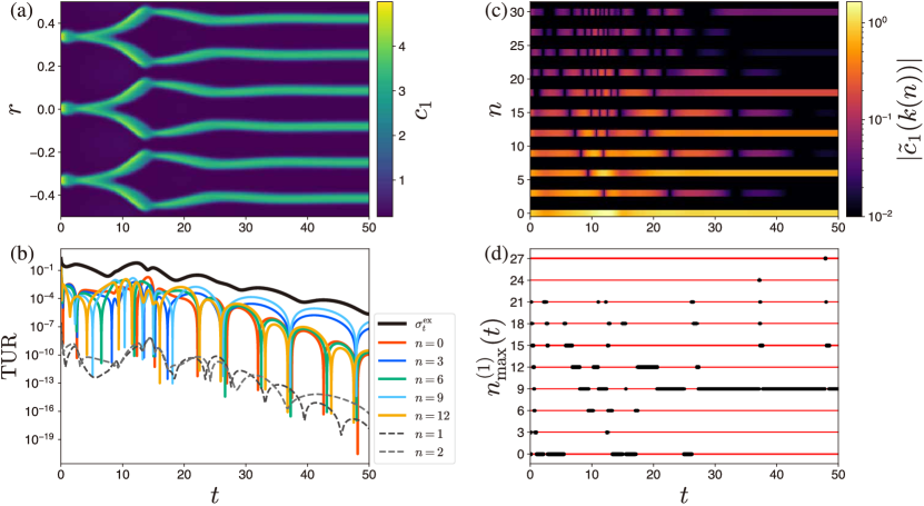
Figure 12: (a) The time series of $c_{1}$. The symmetry of the pattern changes from $3$-fold to $6$-fold. (b) The excess EPR (black line) and its lower bounds $\sigma^{\mathrm{TUR}}_{1}\quantity(n;t)$ for various $n$. (c) The time series of $|\tilde{c}_{1}(k(n))|$. We omit $|\tilde{c}_{1}(k(n))|$ for $n\geq 32$. Since the symmetry of the pattern goes from $3$-fold to $6$-fold, $|\tilde{c}_{1}(k(n))|$ decays if $n$ is a multiple of three but not a multiple of six. (d) $n^{(1)}_{\mathrm{max}}(t)$ (black dots). Reflecting the symmetry of the pattern, $n^{(1)}_{\mathrm{max}}(t)$ is multiples of three (red lines) for all time $t$. Near the stationary pattern ($t>20$), $n^{(1)}_{\mathrm{max}}(t)$ is nine for almost all $t$.

References

- Fuseya et al. [2021] Y. Fuseya, H. Katsuno, K. Behnia, and A. Kapitulnik, Nanoscale turing patterns in a bismuth monolayer, Nature Physics 17, 1031 (2021).
- Asaba et al. [2023] T. Asaba, L. Peng, T. Ono, S. Akutagawa, I. Tanaka, H. Murayama, S. Suetsugu, A. Razpopov, Y. Kasahara, T. Terashima, et al., Growth of self-integrated atomic quantum wires and junctions of a mott semiconductor, Science Advances 9, eabq5561 (2023).
- Belousov [1958] B. P. Belousov, A periodic reaction and its mechanism, Ref. Radiats. Med. (1958).
- Huang et al. [2003] K. C. Huang, Y. Meir, and N. S. Wingreen, Dynamic structures in escherichia coli: spontaneous formation of mine rings and mind polar zones, Proceedings of the National Academy of Sciences 100, 12724 (2003).
- Kondo and Miura [2010] S. Kondo and T. Miura, Reaction-diffusion model as a framework for understanding biological pattern formation, science 329, 1616 (2010).
- Murray [2003] J. D. Murray, Mathematical Biology: II: Spatial Models and Biomedical Applications (Springer New York, 2003).
- Fisher [1937] R. A. Fisher, The wave of advance of advantageous genes, Annals of eugenics 7, 355 (1937).
- Turing [1952] A. M. Turing, The chemical basis of morphogenesis, Philosophical Transactions of the Royal Society of London. Series B, Biological Sciences 237, 37 (1952).
- Kuramoto [1984] Y. Kuramoto, Chemical Oscillations, Waves, and Turbulence (Springer Berlin Heidelberg, 1984).
- Cross and Hohenberg [1993] M. C. Cross and P. C. Hohenberg, Pattern formation outside of equilibrium, Reviews of modern physics 65, 851 (1993).
- Glansdorff and Prigogine [1971] P. Glansdorff and I. Prigogine, Thermodynamic theory of structure, stability and fluctuations (John Wiley and Sons Ltd, 1971).
- Nicolis and Prigogine [1977] G. Nicolis and I. Prigogine, Self-Organization in Nonequilibrium Systems: From Dissipative Structures to Order Through Fluctuations (Wiley-Blackwell, 1977).
- Irvin and Ross [1988] B. R. Irvin and J. Ross, Calculation of the rate of entropy production for a model chemical reaction, The Journal of Chemical Physics 89, 1064 (1988).
- Hanson [1974] M. P. Hanson, Spatial structures in dissipative systems, The Journal of Chemical Physics 60, 3210 (1974).
- Mahara et al. [2004] H. Mahara, N. J. Suematsu, T. Yamaguchi, K. Ohgane, Y. Nishiura, and M. Shimomura, Three-variable reversible gray–scott model, The Journal of Chemical Physics 121, 8968 (2004).
- Mahara and Yamaguchi [2010] H. Mahara and T. Yamaguchi, Entropy balance in distributed reversible gray–scott model, Physica D: Nonlinear Phenomena 239, 729 (2010).
- Falasco et al. [2018] G. Falasco, R. Rao, and M. Esposito, Information thermodynamics of turing patterns, Physical review letters 121, 108301 (2018).
- Rao and Esposito [2016] R. Rao and M. Esposito, Nonequilibrium thermodynamics of chemical reaction networks: Wisdom from stochastic thermodynamics, Physical Review X 6, 041064 (2016).
- Ge and Qian [2016] H. Ge and H. Qian, Mesoscopic kinetic basis of macroscopic chemical thermodynamics: A mathematical theory, Physical Review E 94, 052150 (2016).
- Sekimoto [2010] K. Sekimoto, Stochastic Energetics (Springer Berlin Heidelberg, 2010).
- Seifert [2012] U. Seifert, Stochastic thermodynamics, fluctuation theorems and molecular machines, Reports on progress in physics 75, 126001 (2012).
- Avanzini et al. [2019] F. Avanzini, G. Falasco, and M. Esposito, Thermodynamics of chemical waves, The Journal of Chemical Physics 151 (2019).
- Liang et al. [2022] S. Liang, P. D. L. Rios, and D. M. Busiello, Universal thermodynamic bounds on symmetry breaking in biochemical systems, arXiv preprint arXiv:2212.12074 (2022).
- Miangolarra and Castellana [2023] A. M. Miangolarra and M. Castellana, On non-ideal chemical-reaction networks and phase separation, Journal of Statistical Physics 190, 23 (2023).
- Oono and Paniconi [1998] Y. Oono and M. Paniconi, Steady state thermodynamics, Progress of Theoretical Physics Supplement 130, 29 (1998).
- Hatano and Sasa [2001] T. Hatano and S.-i. Sasa, Steady-state thermodynamics of langevin systems, Physical review letters 86, 3463 (2001).
- Esposito and Van den Broeck [2010] M. Esposito and C. Van den Broeck, Three detailed fluctuation theorems, Physical review letters 104, 090601 (2010).
- Maes and Netočnỳ [2014] C. Maes and K. Netočnỳ, A nonequilibrium extension of the clausius heat theorem, Journal of Statistical Physics 154, 188 (2014).
- Dechant et al. [2022a] A. Dechant, S.-i. Sasa, and S. Ito, Geometric decomposition of entropy production into excess, housekeeping, and coupling parts, Physical Review E 106, 024125 (2022a).
- Dechant et al. [2022b] A. Dechant, S.-i. Sasa, and S. Ito, Geometric decomposition of entropy production in out-of-equilibrium systems, Physical Review Research 4, L012034 (2022b).
- Barato and Seifert [2015] A. C. Barato and U. Seifert, Thermodynamic uncertainty relation for biomolecular processes, Physical review letters 114, 158101 (2015).
- Horowitz and Gingrich [2020] J. M. Horowitz and T. R. Gingrich, Thermodynamic uncertainty relations constrain non-equilibrium fluctuations, Nature Physics 16, 15 (2020).
- Aurell et al. [2011] E. Aurell, C. Mejía-Monasterio, and P. Muratore-Ginanneschi, Optimal protocols and optimal transport in stochastic thermodynamics, Physical review letters 106, 250601 (2011).
- Aurell et al. [2012] E. Aurell, K. Gawȩdzki, C. Mejía-Monasterio, R. Mohayaee, and P. Muratore-Ginanneschi, Refined second law of thermodynamics for fast random processes, Journal of statistical physics 147, 487 (2012).
- Shiraishi et al. [2018] N. Shiraishi, K. Funo, and K. Saito, Speed limit for classical stochastic processes, Physical review letters 121, 070601 (2018).
- Dechant and Sakurai [2019] A. Dechant and Y. Sakurai, Thermodynamic interpretation of wasserstein distance, arXiv preprint arXiv:1912.08405 (2019).
- Nakazato and Ito [2021] M. Nakazato and S. Ito, Geometrical aspects of entropy production in stochastic thermodynamics based on wasserstein distance, Physical Review Research 3, 043093 (2021).
- Van Vu and Hasegawa [2021] T. Van Vu and Y. Hasegawa, Geometrical bounds of the irreversibility in markovian systems, Physical Review Letters 126, 010601 (2021).
- Dechant [2022] A. Dechant, Minimum entropy production, detailed balance and wasserstein distance for continuous-time markov processes, Journal of Physics A: Mathematical and Theoretical 55, 094001 (2022).
- Yoshimura et al. [2023] K. Yoshimura, A. Kolchinsky, A. Dechant, and S. Ito, Housekeeping and excess entropy production for general nonlinear dynamics, Physical Review Research 5, 013017 (2023).
- Van Vu and Saito [2023a] T. Van Vu and K. Saito, Thermodynamic unification of optimal transport: thermodynamic uncertainty relation, minimum dissipation, and thermodynamic speed limits, Physical Review X 13, 011013 (2023a).
- [42] A. Kolchinsky, A. Dechant, K. Yoshimura, and S. Ito, Information geometry of excess and housekeeping entropy production, arXiv preprint arXiv:2206.14599 .
- Van Vu and Saito [2023b] T. Van Vu and K. Saito, Topological speed limit, Physical review letters 130, 010402 (2023b).
- Miangolarra et al. [2023] O. M. Miangolarra, A. Taghvaei, and T. T. Georgiou, Minimal entropy production in the presence of anisotropic fluctuations, arXiv preprint arXiv:2302.04401 (2023).
- Chennakesavalu and Rotskoff [2023] S. Chennakesavalu and G. M. Rotskoff, Unified, geometric framework for nonequilibrium protocol optimization, Physical Review Letters 130, 107101 (2023).
- Villani et al. [2009] C. Villani et al., Optimal transport: old and new, Vol. 338 (Springer, 2009).
- Schiebinger et al. [2019] G. Schiebinger, J. Shu, M. Tabaka, B. Cleary, V. Subramanian, A. Solomon, J. Gould, S. Liu, S. Lin, P. Berube, et al., Optimal-transport analysis of single-cell gene expression identifies developmental trajectories in reprogramming, Cell 176, 928 (2019).
- Arjovsky et al. [2017] M. Arjovsky, S. Chintala, and L. Bottou, Wasserstein generative adversarial networks, in Proceedings of the 34th International Conference on Machine Learning, Proceedings of Machine Learning Research, Vol. 70, edited by D. Precup and Y. W. Teh (PMLR, 2017) pp. 214–223.
- Peyré et al. [2019] G. Peyré, M. Cuturi, et al., Computational optimal transport: With applications to data science, Foundations and Trends® in Machine Learning 11, 355 (2019).
- Benamou and Brenier [2000] J.-D. Benamou and Y. Brenier, A computational fluid mechanics solution to the monge-kantorovich mass transfer problem, Numerische Mathematik 84, 375 (2000).
- Fu et al. [2021] R. Fu, A. Taghvaei, Y. Chen, and T. T. Georgiou, Maximal power output of a stochastic thermodynamic engine, Automatica 123, 109366 (2021).
- Miangolarra et al. [2022] O. M. Miangolarra, A. Taghvaei, Y. Chen, and T. T. Georgiou, Geometry of finite-time thermodynamic cycles with anisotropic thermal fluctuations, IEEE Control Systems Letters 6, 3409 (2022).
- Fujimoto and Ito [2021] Y. Fujimoto and S. Ito, Game-theoretical approach to minimum entropy productions in information thermodynamics, arXiv preprint arXiv:2112.14035 (2021).
- Nagase and Sagawa [2023] R. Nagase and T. Sagawa, Thermodynamically optimal information gain in finite time measurement, arXiv e-prints , arXiv (2023).
- Ito [2023] S. Ito, Geometric thermodynamics for the fokker–planck equation: stochastic thermodynamic links between information geometry and optimal transport, Information Geometry , 1 (2023).
- Kobayashi et al. [2022] T. J. Kobayashi, D. Loutchko, A. Kamimura, and Y. Sughiyama, Hessian geometry of nonequilibrium chemical reaction networks and entropy production decompositions, Physical Review Research 4, 033208 (2022).
- Yoshimura and Ito [2023] K. Yoshimura and S. Ito, Geometric housekeeping–excess decomposition for hydrodynamic systems, arXiv preprint arXiv:2305.19519 (2023).
- Yoshimura and Ito [2021] K. Yoshimura and S. Ito, Thermodynamic uncertainty relation and thermodynamic speed limit in deterministic chemical reaction networks, Physical review letters 127, 160601 (2021).
- Liero and Mielke [2013] M. Liero and A. Mielke, Gradient structures and geodesic convexity for reaction–diffusion systems, Philosophical Transactions of the Royal Society A: Mathematical, Physical and Engineering Sciences 371, 20120346 (2013).
- Liero et al. [2016] M. Liero, A. Mielke, and G. Savaré, Optimal transport in competition with reaction: The hellinger–kantorovich distance and geodesic curves, SIAM Journal on Mathematical Analysis 48, 2869 (2016).
- Dolbeault et al. [2009] J. Dolbeault, B. Nazaret, and G. Savaré, A new class of transport distances between measures, Calculus of Variations and Partial Differential Equations 34, 193 (2009).
- Graps [1995] A. Graps, An introduction to wavelets, IEEE computational science and engineering 2, 50 (1995).
- Torrence and Compo [1998] C. Torrence and G. P. Compo, A practical guide to wavelet analysis, Bulletin of the American Meteorological society 79, 61 (1998).
- Nardini et al. [2017] C. Nardini, É. Fodor, E. Tjhung, F. Van Wijland, J. Tailleur, and M. E. Cates, Entropy production in field theories without time-reversal symmetry: quantifying the non-equilibrium character of active matter, Physical Review X 7, 021007 (2017).
- Harada and Sasa [2005] T. Harada and S.-i. Sasa, Equality connecting energy dissipation with a violation of the fluctuation-response relation, Physical review letters 95, 130602 (2005).
- Ambrosio et al. [2005] L. Ambrosio, N. Gigli, and G. Savaré, Gradient flows: in metric spaces and in the space of probability measures (Springer Science & Business Media, 2005).
- Brasco [2012] L. Brasco, A survey on dynamical transport distances, Journal of Mathematical Sciences 181, 755 (2012).
- Evans and Gangbo [1999] L. C. Evans and W. Gangbo, Differential equations methods for the Monge-Kantorovich mass transfer problem (American Mathematical Soc., 1999).
- Chen et al. [2017] Y. Chen, T. T. Georgiou, L. Ning, and A. Tannenbaum, Matricial wasserstein-1 distance, IEEE control systems letters 1, 14 (2017).
- Rao [1992] C. R. Rao, Information and the accuracy attainable in the estimation of statistical parameters, in Breakthroughs in Statistics: Foundations and basic theory (Springer, 1992) pp. 235–247.
- Ito and Dechant [2020] S. Ito and A. Dechant, Stochastic time evolution, information geometry, and the cramér-rao bound, Physical Review X 10, 021056 (2020).
- Nicholson et al. [2020] S. B. Nicholson, L. P. García-Pintos, A. del Campo, and J. R. Green, Time–information uncertainty relations in thermodynamics, Nature Physics 16, 1211 (2020).
- Griepentrog [2004] J. A. Griepentrog, On the unique solvability of a nonlocal phase separation problem for multicomponent systems (WIAS, 2004).
- Onsager [1931] L. Onsager, Reciprocal relations in irreversible processes. i., Physical review 37, 405 (1931).
- Maes and Netočný [2008] C. Maes and K. Netočný, Canonical structure of dynamical fluctuations in mesoscopic nonequilibrium steady states, Europhys. Lett. 82, 30003 (2008).
- Maes [2018] C. Maes, Non-Dissipative Effects in Nonequilibrium Systems (Springer International Publishing, 2018).
- Murray [2002] J. D. Murray, Mathematical biology: I. an introduction. interdisciplinary applied mathematics, Interdisciplinary Applied Mathematics 10.1007/b98868 (2002).
- Luenberger [1997] D. G. Luenberger, Optimization by vector space methods (John Wiley & Sons, 1997).
- Boyd and Vandenberghe [2004] S. Boyd and L. Vandenberghe, Convex Optimization (Cambridge University Press, 2004).
- Maas [2011] J. Maas, Gradient flows of the entropy for finite markov chains, Journal of Functional Analysis 261, 2250 (2011).
- Feinberg [2019] M. Feinberg, Foundations of chemical reaction network theory, Applied Mathematical Sciences 10.1007/978-3-030-03858-8 (2019).
- Chambolle and Pock [2011] A. Chambolle and T. Pock, A first-order primal-dual algorithm for convex problems with applications to imaging, Journal of mathematical imaging and vision 40, 120 (2011).
- Li et al. [2018] W. Li, E. K. Ryu, S. Osher, W. Yin, and W. Gangbo, A parallel method for earth mover’s distance, Journal of Scientific Computing 75, 182 (2018).
- Otsubo et al. [2020] S. Otsubo, S. Ito, A. Dechant, and T. Sagawa, Estimating entropy production by machine learning of short-time fluctuating currents, Physical Review E 101, 062106 (2020).
- Manikandan et al. [2020] S. K. Manikandan, D. Gupta, and S. Krishnamurthy, Inferring entropy production from short experiments, Physical review letters 124, 120603 (2020).
- Zimmermann and Seifert [2012] E. Zimmermann and U. Seifert, Efficiencies of a molecular motor: a generic hybrid model applied to the f1-atpase, New Journal of Physics 14, 103023 (2012).
- Plaza et al. [2004] R. G. Plaza, F. Sanchez-Garduno, P. Padilla, R. A. Barrio, and P. K. Maini, The effect of growth and curvature on pattern formation, Journal of dynamics and differential equations 16, 1093 (2004).
- Nishide and Ishihara [2022] R. Nishide and S. Ishihara, Pattern propagation driven by surface curvature, Physical Review Letters 128, 224101 (2022).
- Othmer and Scriven [1971] H. G. Othmer and L. Scriven, Instability and dynamic pattern in cellular networks, Journal of theoretical biology 32, 507 (1971).
- Nakao and Mikhailov [2010] H. Nakao and A. S. Mikhailov, Turing patterns in network-organized activator–inhibitor systems, Nature Physics 6, 544 (2010).
- Mielke [2011] A. Mielke, A gradient structure for reaction–diffusion systems and for energy-drift-diffusion systems, Nonlinearity 24, 1329 (2011).