PISA: Point-cloud-based Instructed Scene Augmentation

Abstract

Indoor scene augmentation has become an emerging topic in the field of computer vision with applications in augmented and virtual reality. However, existing scene augmentation methods mostly require a pre-built object database with a given position as the desired location. In this paper, we propose the first end-to-end multi-modal deep neural network that can generate point cloud objects consistent with their surroundings, conditioned on text instructions. Our model generates a seemly object in the appropriate position based on the inputs of a query and point clouds, thereby enabling the creation of new scenarios involving previously unseen layouts of objects. Database of pre-stored CAD models is no longer needed. We use Point-E as our generative model and introduce methods including quantified position prediction and Top-K estimation to mitigate the false negative problems caused by ambiguous language description. Moreover, we evaluate the ability of our model by demonstrating the diversity of generated objects, the effectiveness of instruction, and quantitative metric results, which collectively indicate that our model is capable of generating realistic in-door objects. For a more thorough evaluation, we also incorporate visual grounding as a metric to assess the quality of the scenes generated by our model. The project is available at https://github.com/MRTater/PISA.

1 Introduction

In the rapidly evolving field of computer vision, the significance of 3D computer vision has reached unprecedented heights. It poses many challenges that are similar to those in 2D image processing, but also offers the opportunity to leverage successful strategies from the 2D domain. One such strategy is data augmentation, which aims to enhance the diversity and richness of data. As the demand for 3D data to train models intensifies, so does the need for robust data augmentation techniques. In response to this need, scene augmentation was introduced.

Scene augmentation aims to augment 3D inputs by incorporating new objects that are congruent with their surroundings. It creates new scenarios with previously unseen layouts of objects, thereby enriching the geometrical and auxiliary color features of the training samples. For instance, as depicted in Fig. 1, given a specific scene and query, an object that harmonizes with its surroundings should be generated and inserted in the correct place by the model.

Scene augmentation also has a wide range of applications in industries. It plays a crucial role in the fields of Augmented Reality (AR) and Virtual Reality (VR). In AR, it is used to superimpose virtual objects onto the real world, enhancing the user’s perception and interaction with their environment [21]. In VR, scene augmentation is used to create immersive virtual environments. It can generate diverse scenarios by adding or modifying objects in a virtual scene, enriching the user’s experience. Nevertheless, in today’s VR and AR software development process, it is necessary to have a relatively large material library to insert different types of objects into the scene. Our method, however, allows developers and artists to create realistic and consistent objects directly using simple text prompts, freeing up large amounts of storage and reducing time costs.

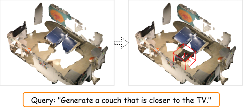
Figure 1: PISA generates a couch that is positioned at a closer distance to the television in response to the query and makes it consistent with the rest of the scene, i.e., the orientation, size, and overlap with other objects in certain cases.

In this paper, we focus on 3D scene augmentation of point clouds, in which point clouds serve as the fundamental building blocks for creating complex and detailed 3D objects. Previous works on point cloud augmentation mainly focus on the transformation of a single object [20] or generating point clouds from existing ones [23]. Some works on scene augmentation reply on inserting pre-built CAD objects into scene [38, 28, 33, 34]. While scene augmentation can be simplified to selection and insertion as a two-stage pipeline, this may result in inflexibility and inconsistency with the surroundings, and only a few works address the issue of generating new objects and incorporating them into scenes as an end-to-end process.

To address these limitations, we propose the Point-cloud-based Instructed Scene Augmentation (PISA), an end-to-end multi-modal deep neural network. PISA can generate objects consistent with the surroundings and integrate these objects seamlessly into given scenes, conditioned on text instructions. This work introduced a unique data pipeline, empowered by GPT, to transform existing visual grounding datasets in order to apply them to the task of instructed scene augmentation (Sec. 3.1). Moreover, a feature fusion module has been designed for space-text feature fusion. After extracting the spatial features from the 3D scene and textual features from the text query, these features will be fused as fusion features. The fusion features, derived from the cross-attention mechanism, capture high-level information from both the surroundings and the query texts, enabling conditional object generation and the location prediction of target point clouds (Secs. 3.2, 3.3 and 3.4).

The effectiveness of our proposed method is validated through qualitative and quantitative experiments conducted on the ReferIt3D dataset [2] (Sec. 4). This work, therefore, presents a significant contribution to this field by addressing previous limitations and proposing innovative solutions.

In summary, the contributions of our work are as follows:

• We design a GPT-aided data pipeline for paraphrasing the descriptive texts in ReferIt3D dataset to generative instructions, referred to Nr3D-SA and Sr3D-SA datasets.

• We propose an end-to-end multi-modal diffusion-based deep neural network model for generating in-door 3D objects into specific scenes according to input instructions.

• We propose quantified position prediction, a simple but effective technique to predict Top-K candidate positions, which mitigates false negative problems arising from the ambiguity of language and provides reasonable options.

• We introduce the visual grounding task as an evaluation strategy to assess the quality of an augmented scene and integrate several metrics to evaluate the generated objects.

2 Related Work

Text-guided 3D Vision.

While 2D text-guided tasks have achieved great success in recent years, 3D text-guided tasks also hold a high degree of research interest. The majority of 3D V+L tasks are derived from corresponding 2D tasks as an extension of 2D space to 3D space, such as 3D visual grounding [2, 6, 41, 15], 3D dense captioning [9, 17, 8], and 3D shape generation [7, 22, 39]. Despite the differences between these 3D V+L settings, these tasks are generally dependent on the 3D features and text features extracted from the 3D settings and guidance text to adapt the downstream tasks in a classic encoder-decoder manner. In early works [2, 6], 3D scene features are combined with text features through direct concatenation for downstream classifiers. Since attention mechanisms have proven to be successful in deep learning, many recent works [8, 15, 18, 42] have adopted transformer-based decoders as fusion module to improve performance and achieve better results.

Scene Augmentation.

The field of scene augmentation has witnessed substantial progress in recent years. [44] uses GNN to construct the relationships between objects and their surroundings. Building on this, [38] introduce a method for inserting objects from CAD models into predicted position based on the text prompt. Similarly, [33, 34, 28] utilized object selection and insertion techniques, simplifying the problem of scene generation to a selection of objects from the database and pose predictions for each object. However, a significant limitation of these methods is their heavy reliance on pre-generated point clouds or pre-stored CAD models. This dependence often results in inconsistencies with the surrounding environment and hampers seamless integration into scenes. Furthermore, this approach restricts the variety of objects that can be generated, contradicting the initial objective of accommodating open-ended text prompts. This constraint underscores the need for more flexible and adaptive techniques in scene augmentation, capable of generating a wider array of objects while ensuring harmonious integration with the existing environment. There are also some works [3, 32, 14] that are built based on neural radiance fields [25] that can synthesize indoor scenarios. However, these methods usually need images as input and the camera views of images are strictly restricted, which may not be feasible for certain tasks.

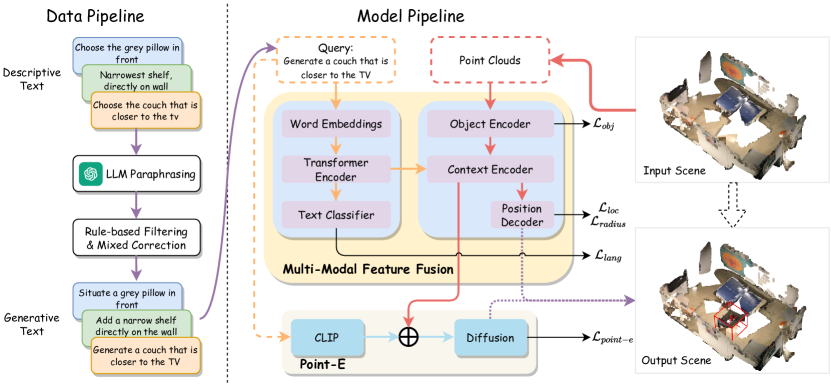
Figure 2: Overview of Point-cloud-based Instructed Scene Augmentation (PISA). (a) A large language model (LLM) is used to paraphrase the descriptive text, combined with rule-based and manual corrections. (b) Upon receiving generative text as a query and point cloud input, our model integrates both object and language features to predict the final position. The amalgamated features are then processed through the Point-E model to generate a realistic object.

Point Cloud Generation.

Many prior works have explored generative models over point clouds, including the use of autoencoder [1], flow-based generation [40], and generative adversarial neural networks (GAN) [16]. Besides, the Diffusion Model [36, 13], which has been proven to have great potential in the generative field, are widely applied. [23] treated point clouds as samples from a point distribution and reverse diffusion Markov chain to model the distribution of point. [43] introduce PVD, a diffusion model that generates point clouds directly instead of translating a latent vector to a shape. Yet, these studies did not demonstrate the capability to generate point clouds conditioned on open-ended text prompts. More recently, OpenAI introduced Point-E [26], a sophisticated model predicated on the concept of conditional diffusion, uniquely designed to generate point clouds directly, bypassing the need for latent vector translation. Point-E is also capable of producing colored point clouds in response to intricate text or image prompts, showcasing an impressive degree of generalization across a multitude of shape categories. Our object generation model is built upon the robust foundation provided by Point-E, capitalizing on its pre-trained model to enhance our system’s capabilities.

3 Methodology

In this section, we introduce the proposed Point-cloud-based Instructed Scene Augmentation (PISA). An overview of our model is presented in Fig. 2.

Data Pipeline.

We transform the existing visual grounding dataset to accommodate the task of instructed scene augmentation. As part of the data pipeline, descriptive texts are paraphrased by LLM to obtain generative instructions, which are then revised manually and by rules.

Model Pipeline.

The scene augmentation process involves two stages: (a) locate the desired position using the grounding model; (b) create a new object based on the location and scene context using the text-to-point model. In the following sections, we will elaborate further on each module.

Problem Statement.

The instructed scene augmentation task is to generate a proper target object $O_{tgt}$ into a specific scene $S$ given a generative instruction. In our settings, a scene $S$ can be viewed as the collection of the in-scene objects $\{O_{ctx,i}\}^{N}_{i=1}$. The spatial representation of an object $O$ can be viewed as the combination of the center location $\bm{l}\in\mathbb{R}^{3}$, the original size $s\in\mathbb{R}$, and the normalized point cloud $\mathbf{p}\in[-1,1]^{P\times C}$. For simplicity, we rewrite $S$ as:

$$\mathbf{L}\in\mathbb{R}^{N\times 3},\bm{s}\in\mathbb{R}^{N},\mathbf{P}\in[-1,1]^{N\times P\times C}$$ (1)

where $N$ is the number of in-scene context objects and $C$ is the number of channels (e.g., $C=6$ for XYZ-RGB points).

3.1 Dataset Transformation

To adapt the instructed scene augmentation task, our method transforms the ReferIt3D dataset [2] as shown in data pipeline. ReferIt3D dataset consists of 41K manually labeled (Nr3D dataset) and 114K machine-generated (Sr3D dataset) descriptions of specific targets in given scenes of the ScanNet dataset [10]. Each description entry illustrates the in-door location, type, and shape of the target object. Since the ReferIt3D dataset only contains descriptive texts, we leverage the GPT-3.5 [4] to paraphrase them into generative instructions. The transformed datasets are noted as Nr3D-SA and Sr3D-SA, containing a total of 155K generative instructions for 76 object classes, involving 1436 different scene scans of the ScanNet dataset.

Prompt engineering is used to facilitate the paraphrasing process. We construct well-designed prompting templates to instruct GPT-3.5 to perform paraphrasing. It should also be noted that human-labeled descriptions of Nr3D are generally more complex than those generated by machines of Sr3D. Even humans have difficulty distinguishing the correctly paraphrased ones from the incorrect ones. Therefore, we employ rule-based techniques to filter out the errors produced by GPT-3.5. The errors are then revised through an additional GPT-4 [27] round with manual corrections.

Detailed information regarding the prompt-based paraphrasing process, including the prompting templates and filtering rules, can be found in the Supplementary Material.

3.2 Multi-Modal Context Fusion

To accomplish multi-modal feature fusion, we decouple the fusion process into two steps, i.e., feature extraction and cross-attention fusion.

Feature Extraction.

Point cloud features of all context objects are extracted by the object encoder. In practice, we use PointNeXt [30] rather than the commonly used PointNet++ [29]. For the language features of the query text, we adopt a Transformer Encoder-based language model (e.g., BERT [19]). Since the query text is relatively simple, only part of the encoder layers can handle language modeling. The object encoder and the text encoder produce the point cloud and textual features as $\mathbf{x}_{obj}\in\mathbb{R}^{N\times D}$ and $\mathbf{x}_{lang}\in\mathbb{R}^{T\times D}$, respectively. The dimension of the latent representation is $D$ whereas the token size of query text is $T$.

Cross-attention Fusion.

The multi-modal features are fused by the object feature $\mathbf{x}_{obj}$ and the query feature $\mathbf{x}_{lang}$ using the cross-attention mechanism [37]. We adopt a standard Transformer Decoder as the context encoder. Prior to the cross-attention, a learnable token [CTX] is prepended to the front of object features as $\bm{x}_{ctx}\in\mathbb{R}^{D}$. Also, an additional object position embedding is applied to provide spatial information to the context encoder:

$$\mathrm{PE}(\mathbf{L},\bm{s})=\mathrm{LayerNorm}(\operatorname{MLP}([\mathbf{L}\mathbin{\|}\bm{s}]))$$ (2)

The multi-modal features are then calculated as:

$$\mathbf{x}_{mm}=\mathrm{XAttn}([\bm{x}_{ctx}\mathbin{\|}\mathbf{x}_{obj}]+\mathrm{PE}(\mathbf{L},\bm{s}),\mathbf{x}_{lang})$$ (3)

where $\mathrm{XAttn}$ is cross-attention encoder, $\cdot\mathbin{\|}\cdot$ is the concatenation operator, and $\operatorname{MLP}$ is the Multi-Layer Perceptrons.

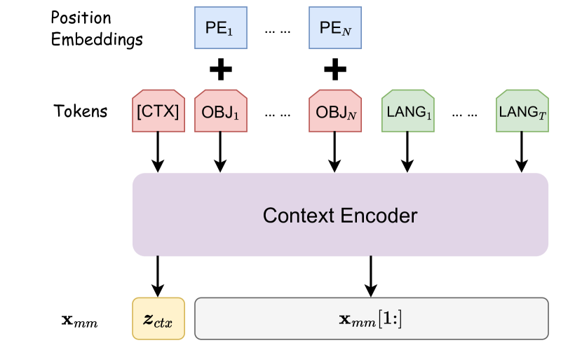
Figure 3: Extraction of context vector $\bm{z}_{ctx}$.

The cross-attention mechanism integrates both the spatial feature of context objects and the query text feature. Alternatively, it can be considered a ”scene encoder” that extracts the features from both the query text and the scene. As shown in Fig. 3, the context vector $\bm{z}_{ctx}$ representing the entire scene and query is then extracted from the first token of $\mathbf{x}_{mm}$, corresponding to the position of the token [CTX].

3.3 Quantified Position Prediction

Given the inherent ambiguity and potential vagueness of many queries, predicting the location of objects poses a significant challenge for our model, as evidenced by our experimental results in Tab. 3, we introduce a technique known as quantified position prediction (QPP). This fundamental concept entails the transformation of a continuous coordinate system into discrete bins, thereby simplifying the intricate regression problem into an easier classification task.

We divide the space into discrete bins and train the model to predict the normalized $xyz$ coordinates within each bin. The division procedure can be formulated as:

$$\tilde{\bm{l}}=\left\lfloor\frac{\bm{l}-\min_{xyz}}{\max_{xyz}-\min_{xyz}}\times B\right\rfloor$$ (4)

where $\tilde{\bm{l}}$ is the normalized bin coordinate, $\bm{l}$ is the original coordinate, $\lfloor\cdot\rfloor$ is the floor rounding function, $\max_{xyz}$ and $\min_{xyz}$ represent the maximum and minimum coordinate of each axis respectively, and $B$ is the total number of bins.

Furthermore, our practical experiments have revealed that objects within the same class often exhibit substantial variations in the $xy$-plane but tend to have similar $z$ coordinates. Thus, we separate the prediction process into two parts: one that addresses the $xy$-plane bin prediction and the other that addresses the $z$-axis bin prediction, and then concatenate them, formulated as follows:

$$\begin{gathered}\hat{\bm{l}}_{xy}=\operatorname{MLP}(\bm{z}_{ctx}),~{}\hat{\bm{l}}_{z}=\operatorname{MLP}(\bm{z}_{ctx})\\ \hat{\bm{l}}=[\hat{\bm{l}}_{xy}\mathbin{\|}\hat{\bm{l}}_{z}]\end{gathered}$$ (5)

where $\hat{\bm{l}}$ is the predicted normalized coordinates. This normalized position is then restored to the original space’s coordinates as the final predicted location.

3.4 Context-Aware Point Cloud Generation

We utilize the Point-E model [26] as our point cloud generation model. Point-E is a generative model developed by OpenAI for generating 3D point clouds from complex prompts based on Diffusion. We use the pre-trained model base40M-textvec provided by Point-E, which has been trained on ShapeNet [5]. Point-E’s diffusion process, which is similar to other diffusion models, aims to sample from some normal distribution $q(\bm{x}_{0})$ using a neural network approximation $p_{\theta}(\bm{x}_{0})$.

In Point-E, guidance is used as a trade-off between sample diversity and fidelity in diffusion. Point-E inherits the classifier-free guidance from [12], where a conditional diffusion model is trained with the class label stochastically dropped and replaced with an additional Ø, using the drop probability 0.1. During the sampling, the model’s output $\epsilon$ is linearly extrapolated away from the unconditional prediction towards the conditional prediction:

$$\hat{\epsilon}_{guided}=\epsilon_{\theta}(\bm{x}_{t},\text{\O})+s\cdot(\epsilon_{\theta}(\bm{x}_{t},\bm{y})-\epsilon_{\theta}(\bm{x}_{t},\text{\O}))$$ (6)

for guidance scale $s\geq 1$.

Several modifications are made to the Point-E model to better adapt it for context-aware generation tasks. One of the key changes involves the integration of context feature vectors $\bm{z}_{ctx}$ with the text feature vectors $\bm{z}_{\text{CLIP}}$ generated by the CLIP model [31] as shown in Fig. 2. This new combined feature vector is then used as input labels in the guided diffusion learning process, formulated as:

$$\bm{y}=\operatorname{MLP}(\bm{z}_{ctx}+\bm{z}_{\text{CLIP}})$$ (7)

The primary objective of this modification is to enable the diffusion model to effectively utilize contextual information from the scene and query text as guidance. This, in turn, allows for the generation of objects that are more harmoniously integrated with their surroundings.

3.5 Loss

The model’s training process involves five distinct losses, four for multi-modal feature fusion and one for Point-E diffusion, as illustrated in Fig. 2.

Firstly, we have the loss $\mathcal{L}_{obj}$, originating from the [15] and tailored for multi-modal feature fusion. Specifically, it is computed as the cross-entropy between the predicted object type of all context objects from the object feature $\mathbf{x}_{obj}$ and their ground truths.

Next, we have the loss $\mathcal{L}_{lang}$, which measures the discrepancy between the predicted type of the generated object from the query text feature $\mathbf{x}_{lang}$ and the ground truth.

The third and fourth losses pertain to position prediction, represented by $\mathcal{L}_{loc}$ and $\mathcal{L}_{scale}$. These are supervised cross-entropy loss for target position prediction and L1 loss for object size, respectively. $\mathcal{L}_{loc}$ is the combined loss of two MLPs defined in Eq. 5.

Hence we could define the loss $\mathcal{L}_{mm}$ as the total loss of multi-modal feature fusion:

$$\mathcal{L}_{mm}=\alpha_{obj}\times\mathcal{L}_{obj}+\alpha_{lang}\times\mathcal{L}_{lang}+\mathcal{L}_{loc}+\mathcal{L}_{scale}$$ (8)

where $\alpha_{obj}$ and $\alpha_{lang}$ serve as weights for certain loss terms, both with the default value of $0.5$.

Lastly, for point cloud generation supervision, we inherit the Mean Squared Error (MSE) loss from the Point-E model, denoted as $\mathcal{L}_{point-e}$.

We can therefore calculate the total loss as the sum of all losses during the training process:

$$\mathcal{L}=\mathcal{L}_{mm}+\mathcal{L}_{point-e}$$ (9)

4 Experiments

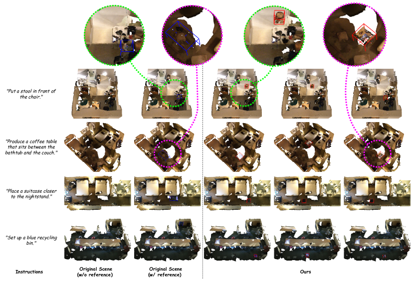
Figure 4: Scenes before and after augmentation. Each row represents the scenes to be augmented under different instructions. Different random seeds are used to generate the columns of the augmented scene. Candidate locations are extracted from the Top-5 predictions. The bounding boxes of reference objects and generated objects are outlined in blue and red, respectively.

4.1 Experimental Setup

Dataset.

We train and evaluate our method on the Nr3D-SA and Sr3D-SA datasets generated in Sec. 3.1. For experiments trained on Nr3D-SA, only query data with explicit reference to the type of the target object is used, while all data is included in the Sr3D-SA settings. The datasets are divided into 80% for training and 20% for evaluation. The target object is separated from the other context objects in the scene and is set as the ground truth during training. In the training stage, we apply a 4-direction random rotation on the scenes. In the evaluation phase, the target object serves as a reference for assessing the generation quality.

Implementation Details.

The dimension $D$ of latent representation throughout the model pipeline is set to 768. For the point cloud encoder backbone, we adopt the PointNeXt-L model based on its state-of-the-art performance [30]. We adopt the pre-trained BERT_BASE [19] with the first three layers as the query text encoder. The context encoder is a four-layer Transformer Decoder for multi-modal feature fusion. The number of quantified bins is set to $B=32$.

We implement our model in PyTorch and deploy point-cloud-based backbone models using the OpenPoints library [30]. Farthest Point Sampling (FPS) algorithm based on QuickFPS [11] is also used for efficient point sampling, with a setting of $P=1024$ as the point cloud size. For the training phase, our model is trained with a batch size of 8 for a total of 800,000 steps on both Nr3D-SA and Sr3D-SA datasets using $\sim$120 RTX3090 GPU hours. We also train our model on only Nr3D-SA for quick verification, with a total of 160,000 steps. For optimization, we use AdamW with hyper-parameters $\beta=(0.95,0.999),\epsilon=10^{-6}$ and weight decay of $10^{-3}$. The base learning rate for multi-modal fusion part and Point-E is $2\times 10^{-4}$ and $4\times 10^{-5}$ respectively, where the learning rate for BERT_BASE and context encoder is set to $\frac{1}{10}$ of the base. Additionally, we employ a linear learning rate schedule from $2\times 10^{-4}$ to $10^{-5}$.

4.2 Metrics

Quality of Generation.

In the context of 3D generation evaluation, Earth Mover’s Distance (EMD) [35] measures the similarity between two point clouds. Following previous works [1, 40, 43], we evaluate the quality of generated point clouds using the metrics of minimum matching distance (MMD), coverage (COV), 1-nearest neighbor accuracy (1-NNA), and Jensen-Shannon Divergence (JSD). A similarity between the distribution of generated and reference point clouds indicates a high degree of realism.

Given the fact that EMD and JSD are only capable of assessing the disparity in point distribution, thus merely providing an indirect evaluation of the generative performance, we propose an auxiliary metric to evaluate the quality of generated objects and the performance of language modeling. We employ a PointNeXt classifier trained on ReferIt3D to classify the generated objects. Furthermore, we observe that objects belonging to certain classes may have analogous shapes, such as suitcases and boxes. To mitigate this problem, we apply the Top-K estimation to classification accuracy, denoted as Acc@$k$. This approach allows us to mitigate the false negatives caused by similar shapes.

Top-K Distance Estimation.

Due to the inherent ambiguity and vagueness in natural language, it is common to encounter multiple potential position matches for a single query. This assortment of possible matches can complicate the task of accurately interpreting and responding to user queries. To address this challenge, we implement a method known as Top-K Distance Estimation, denoted as $\Delta\bm{l}$@$k$.

This method allows the model to gauge its current performance more accurately by considering the Top-K closest match position, rather than relying on a single best match, e.g., IoU. By taking into account a range of closely matching responses, the model can better navigate the nuances and ambiguities of natural language, and thus is less likely to be adversely affected by vague descriptions or queries.

4.3 Experiment Results

Loc.	Shape	Overall(%,$\uparrow$)	Easy(%,$\uparrow$)	Hard(%,$\uparrow$)
Rnd.	Rnd.	3.62	4.76	2.53
Rnd.	P.O.	10.11	13.58	6.78
Rnd.	GT	19.29	23.94	14.83
Rnd.	Ours	12.26	15.90	8.76
GT	Rnd.	11.03	14.41	7.78
GT	P.O.	31.07	36.71	25.64
GT	GT	54.22	61.44	47.28
GT	Ours	40.05	46.78	33.39
Ours	Rnd.	8.08	10.58	5.67
Ours	P.O.	29.42	35.06	24.00
Ours	GT	37.33	46.07	28.92
Ours	Ours	34.14	41.09	27.07

Table 1: Visual grounding analysis of the augmented scene. We employed MVT [15], which was trained using ReferIt3D dataset, as the visual grounding model. Loc. is the location of the target object. Rnd. means either the location or the shape of the target object is randomly generated. P.O. stands for Point-E Only model and GT stands for ground truth.

Object Class	Ours						Point-E Only
	MMD$\downarrow$	COV$\uparrow$	1-NNA$\downarrow$	JSD$\downarrow$	Acc@1$\uparrow$	Acc@5$\uparrow$	MMD$\downarrow$	COV$\uparrow$	1-NNA$\downarrow$	JSD$\downarrow$	Acc@1$\uparrow$	Acc@5$\uparrow$
chair(7.58%)	9.74	38.00	98.64	2.091	63.84	90.75	11.15	21.63	99.63	2.782	62.39	91.56
trash can(4.78%)	9.94	32.84	99.59	2.696	39.26	76.62	11.62	19.37	99.69	3.700	6.77	30.60
window(4.76%)	8.63	34.24	99.76	2.994	39.95	72.49	9.69	27.53	99.77	3.309	39.40	64.27
table(4.70%)	10.23	33.66	99.57	3.219	23.06	54.01	13.20	20.93	99.37	4.614	21.73	45.58
cabinet(3.71%)	9.92	33.36	98.86	2.638	12.49	44.76	10.82	27.64	99.50	2.974	9.21	38.84
picture(3.53%)	6.03	36.30	99.37	2.929	21.38	60.85	6.98	31.24	99.58	3.309	35.01	67.09
shelf(3.42%)	8.16	28.35	99.77	2.695	15.94	44.11	8.79	23.99	99.69	2.910	24.71	48.07
lamp(3.17%)	12.62	26.49	99.73	3.530	29.73	51.89	13.58	24.10	99.86	4.490	12.53	23.28
desk(3.16%)	11.34	31.17	99.90	3.025	14.26	33.24	13.96	22.85	99.85	3.839	1.90	15.33
pillow(2.36%)	9.60	41.81	99.35	2.716	47.74	72.68	10.71	37.24	99.24	3.180	26.58	50.23
backpack(2.34%)	10.38	34.56	98.54	2.172	37.57	76.23	11.54	27.52	99.21	2.414	27.94	68.31
. . .	. . .						. . .
Micro Avg.	10.10	33.69	99.24	3.080	24.10	49.21	11.50	26.87	99.40	3.620	18.37	39.85

Table 2: Snapshot of EMD values and classification accuracy for 32K objects generated from 32K randomly sampled generative texts from the test set, using our method and Point-E without feature fusion separately. Each class’s proportion in the training set is also shown. MMD is multiplied by $10^{2}$ and JSD is multiplied by $10^{1}$.

Ablate	Acc@1$\uparrow$	Acc@5$\uparrow$	$\Delta\bm{l}$@1$\downarrow$	$\Delta\bm{l}$@5$\downarrow$	MMD$\downarrow$	JSD$\downarrow$	$\Delta s\downarrow$	$\text{Acc}_{obj}$$\uparrow$	$\text{Acc}_{lang}$$\uparrow$
Vanilla Transformer + Point-E	18.96	39.34	2.179	-	13.29	3.575	0.161	51.95	89.63
+ FPS	19.30	40.49	2.251	-	12.78	3.455	0.163	51.72	89.71
+ Quantified Position ($B=32$)	23.10	44.23	2.654	1.302	12.37	3.471	0.162	52.07	89.88
+ Quantified Position ($B=16$)	18.93	39.11	2.599	1.264	12.50	3.538	0.163	51.70	89.97
+ Sr3D-SA (Ours)	24.10	49.21	2.125	1.171	10.10	3.080	0.146	55.71	95.22

Table 3: Additive ablation study of sequentially applying different training techniques for Scene Augmentation task. Dash ”-” is used as a placeholder for unavailable results. Acc@$k$ is the Top-$k$ classification accuracy of generated objects, whereas $\text{Acc}_{obj}$ and $\text{Acc}_{lang}$ are the accuracy of categorizing the context objects and instructions. $\Delta\bm{l}$ and $\Delta s$ measures the difference between the predicted and ground truth locations and sizes. MMD is multiplied by $10^{2}$ and JSD is multiplied by $10^{1}$.

Visualization.

Figure 4 visualizes the qualitative results of our method on the evaluation of the Sr3D-SA dataset. The candidate locations of each object are chosen from the Top-5 predictions, while the point cloud is derived using different random seeds. Most of the generated point clouds are located in close proximity to the reference points and the shapes are consistent with the instructions. While some of the generated objects may vary from the references, they are oriented and sized in accordance with their surroundings.

We also observe that several predicted locations deviate from the reference due to the ambiguous instructions, e.g., the results of ”Set up a blue recycling bin”. To reduce the ambiguity of instructions, prepositions of position (e.g., ”in front of the chair”) can be used to limit the possible locations to those nearby desired locations. Generally, locating ability improves when instructions are less ambiguous.

Diversity of Generations.

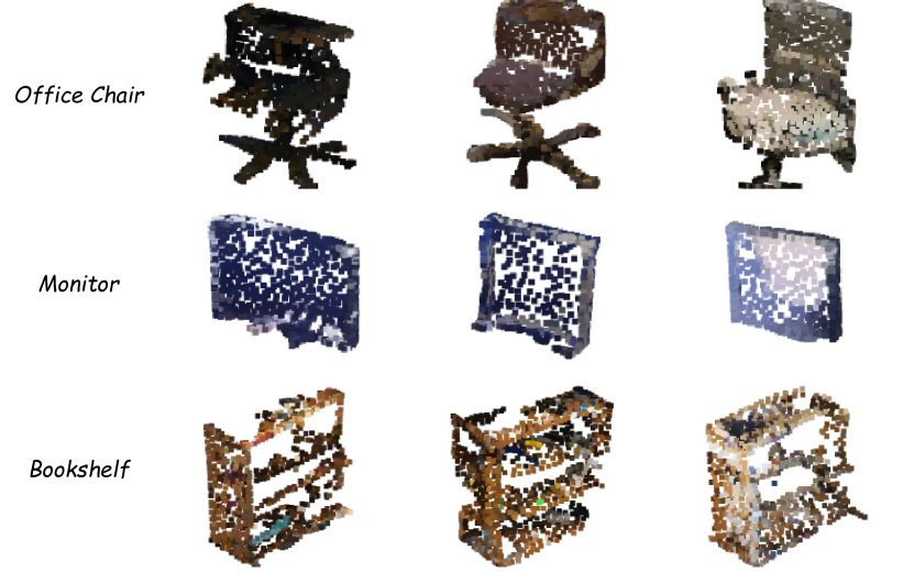
Figure 5: Diversity. The leftmost column shows the category of the generated object to be generated from the instruction. Different generations under the same instruction are shown in each row.

One of the key advantages of our diffusion-based approach to 3D object generation is that diverse shapes can be generated for a given instruction, as shown in Fig. 5. This figure illustrates three distinct categories of point clouds generated from different random seeds. While maintaining consistency with the surrounding environment and instructions, our method creates meaningful variances in both shape and color. It allows the choice of the best shape to be made from a variety of options.

Effectiveness of Instructions.

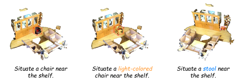
Figure 6: Generated objects under instructions with slight variations. Each target object is created into the scene with a variation in shape or color.

Moreover, since the shape of the generated object is determined by the instructions, the effectiveness of different instructions indicates the generalization ability of our approach. Figure 6 provides results for the generated objects when different instructions are applied with slight variations. These results demonstrate that our approach can capture the differences between instructions while maintaining the semantics of the target object.

Quantitative Result.

To assess the quality of the augmented scene, we employ the MVT model [15] to perform visual grounding task on three distinct scenes: randomly generated scenes, original ReferIt3D scenes, and our augmented scenes, as shown in Tab. 1. The goal of visual grounding is to identify the target object in a scene based on the text provided. There are no distractor objects of the same type as the target one in Easy tasks, whereas multiple objects of the same type are available in Hard tasks.

It is observable that our model is capable of generating scenes that are not only consistent but also easily recognizable by visual grounding models trained on the original dataset. Despite the inherent complexities involved in scene generation, which may lead to a certain degree of decline in overall visual grounding accuracy than the ground truth dataset, our model performs well in generating high-quality scenes. These generated scenes are more identifiable to the visual grounding model compared to those generated randomly or those generated by a single Point-E model with ground truth locations. Performance in Hard tasks also indicates the effectiveness of our approach in complex scenes.

Nevertheless, to conduct a comprehensive assessment of the performance of object generation, we sample 32,000 generative texts from the test set. For each generated object within this sample set, we compute the metrics in Sec. 4.2. We also perform experiments on a single Point-E model to compare the performance of our context-aware design, i.e., Eq. 7, as shown in Tab. 2. The complete results are in the Supplementary Material. It demonstrates that the ability of our model to generate objects is deemed reasonable.

Ablation study.

In this section, we evaluate our method in different settings and strategies. We conduct an additive ablation study on the location and generation quality, as illustrated in Tab. 3. In the baseline model, only Nr3D-SA is used as training data, and the model is built on a bare backbone. Also, we evaluate the accuracy of identifying context objects and instructions in relation to $\mathcal{L}_{obj}$ and $\mathcal{L}_{lang}$. It is noteworthy that the performance of $\Delta\bm{l}$@1 degrades when the quantified position is applied. We observe, however, that the position predictor without quantified position exhibits significant under-fitting: most of the predicted locations remain close to the middle of the scene for a statistically minimal $\Delta\bm{l}$, which contradicts the intended purpose.

5 Discussion

Owing to the constraints of computational resources, we opted to sample 1024 points. Nonetheless, for existing point cloud generation models [24], it is advisable to sample more points (e.g., 4096) to achieve a more real-life outcome. Additionally, enhancing the generative model’s capability may lead to further improvements in our model’s performance. It is also important for our data-driven training process to expand the relatively limited dataset. Our results in the Supplementary Material indicate that the performance is significantly lower for certain classes with less data.

6 Conclusion

In this work, we present the PISA, the first end-to-end multi-modal approach to generate augmented scenes conditioned on instruction. To obtain a proper dataset for scene augmentation, we use prompt engineering in conjunction with large language models to transform existing visual grounding data. Our method then utilizes both spatial and language features from the scene and instructions as guidance to the diffusion and locating processes. Furthermore, the experiment results exhibit the high capability of generating realistic objects at the appropriate locations according to various metrics and the visual grounding analysis. We hope this work will be a step towards the more practical applications of 3D human-computer interactions.

Acknowledge.

K. Lin is supported by National Key R&D Program of China under grant 2022YFB2703001.

Supplementary Material

7 Dataset Transformation

In this section, we provide more details about the data transformation from ReferIt3D to Nr3D-SA and Sr3D-SA. As depicted in Fig. 8, The data pipeline can be summarized as follows. (a) Paraphrase the descriptive texts into generative instructions based on LLM prompt engineering. (b) Filter out erroneous results by rules. (c) Re-paraphrase the incorrect ones using GPT-3.5 or GPT-4 according to the perplexity of sentences. (d) Proofread the revised sentences manually. The steps (b) and (c) are repeated until the rule-based filters detect no errors. After that, the step (d) is performed.

7.1 Prompting Templates

Prompts:
You are a helpful chatbot.
Following sentences locate ONLY ONE object in a scene.
Transform the sentence to create this object.
Include generative verbs such as ’ {I-VERB}’ to create it.
Change ’the’ to ’a’ or ’an’ properly.
Imperative sentences are prefered.
Declarative sentences such as ’there is’ are disallowed.
Avoid multiple imperative sentences.
{TEXT}

Figure 7: Dynamic prompting templates with slots. Imperative verbs {I-VERB} are selected randomly from a manually designed list with weights. The likelihood of preference for imperative sentences are set to $0.5$. The original texts are placed to {TEXT} slot.

To generate diverse instructions without breaking changes in the semantics of original texts, we use dynamic prompting templates with different manually designed imperative verbs. We leverage the ChatGPT [27] API to rewrite each original descriptive text. The prompts for calling the ChatGPT API are shown in Fig. 7. The verbs are selected randomly and inserted into the corresponding slots during each call to the API. A weight is also assigned to each verb to ensure that the language is more natural. The verbs are listed as follows: add (10%), put (10%), place (10%), set (10%), create (10%), generate (10%), insert (10%), produce (10%), lay (5%), deposit (5%), position (5%), and situate (5%). To improve the diversity of the generated instructions (e.g., passive sentences and clauses), we reduce the likelihood of producing imperative sentences to $0.5$.

7.2 Rule-based Filtering

Although LLMs have tremendous power, errors still occur when the original sentences are too complex, particularly for the Nr3D dataset. To detect errors in generated instructions, we employ rule-based filtering methods to identify obvious errors. The following are descriptions of our filtering rules:

1. Locating words that are not transformed properly should be considered erroneous. The word blacklist covers: find, pick, choose, select, locate, identify, search, seek, spot, gaze, etc.

2. Sentences without any generative verbs in Sec. 7.1 should be considered incorrect.

3. Missing negative words and antonyms indicate high risks of changing the semantics of original sentences, such as no, not, nowhere, and nothing.

7.3 Mixed Correction

As a means of revising the error-prone sentences, we propose a mixed correction process involving both GPT and human labor. We first repeat the paraphrasing process on the incorrect sentences. We observe that Sr3D generates much better quality sentences than Nr3D due to its concise grammar structure. Since the proportion of incorrect sentences in Nr3D is smaller than that of the entire dataset, we perform manual proofreading on paraphrased sentences only from Nr3D as the final step. By the end of the process, only 335 sentences out of 41K sentences from Nr3D are required to be manually revised by two workers.

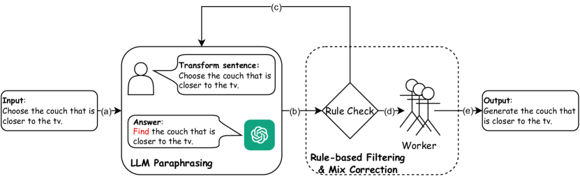
Figure 8: Data pipeline. Input texts are first processed through steps (a) and (b). If the generated texts are considered incorrect, step (c) would be taken to re-run the paraphrasing process until no error is found. After that, manual proofreading and correction are applied as step (d) to output the final results.

8 Additional Experiment Results

Table 4 shows the complete results of EMDs and classification accuracy in response to Sec. 4. The table is sorted according to the proportion of objects within the entire dataset for ease of comparison. It is noteworthy that the classification accuracy is higher for object classes with more data, whereas the performance drops drastically for object classes with less data.

Object Class	Ours						Point-E Only
	MMD	COV	1-NNA	JSD	Acc@1	Acc@5	MMD	COV	1-NNA	JSD	Acc@1	Acc@5
chair(7.58%)	9.74	38.00	98.64	2.091	63.84	90.75	11.15	21.63	99.63	2.782	62.39	91.56
door(6.72%)	6.73	27.83	99.86	2.733	0.76	9.01	7.57	21.39	99.93	2.936	2.16	13.89
trash can(4.78%)	9.94	32.84	99.59	2.696	39.26	76.62	11.62	19.37	99.69	3.700	6.77	30.60
window(4.76%)	8.63	34.24	99.76	2.994	39.95	72.49	9.69	27.53	99.77	3.309	39.40	64.27
table(4.70%)	10.23	33.66	99.57	3.219	23.06	54.01	13.20	20.93	99.37	4.614	21.73	45.58
cabinet(3.71%)	9.92	33.36	98.86	2.638	12.49	44.76	10.82	27.64	99.50	2.974	9.21	38.84
picture(3.53%)	6.03	36.30	99.37	2.929	21.38	60.85	6.98	31.24	99.58	3.309	35.01	67.09
shelf(3.42%)	8.16	28.35	99.77	2.695	15.94	44.11	8.79	23.99	99.69	2.910	24.71	48.07
lamp(3.17%)	12.62	26.49	99.73	3.530	29.73	51.89	13.58	24.10	99.86	4.490	12.53	23.28
desk(3.16%)	11.34	31.17	99.90	3.025	14.26	33.24	13.96	22.85	99.85	3.839	1.90	15.33
pillow(2.36%)	9.60	41.81	99.35	2.716	47.74	72.68	10.71	37.24	99.24	3.180	26.58	50.23
backpack(2.34%)	10.38	34.56	98.54	2.172	37.57	76.23	11.54	27.52	99.21	2.414	27.94	68.31
sink(2.33%)	11.22	29.06	98.97	3.202	68.38	82.74	12.19	25.95	98.96	3.915	41.18	70.59
towel(2.23%)	8.66	30.77	99.76	3.255	9.62	37.18	9.37	29.08	99.66	3.214	7.06	22.35
monitor(2.17%)	8.44	36.70	99.64	3.027	78.82	87.97	8.91	31.31	99.70	3.241	68.21	86.79
box(2.09%)	11.93	41.83	98.78	2.905	38.47	72.21	13.85	28.53	98.87	3.814	7.06	31.98
nightstand(1.77%)	10.95	28.57	98.75	2.971	15.00	49.64	11.86	32.28	99.61	3.868	5.51	50.39
couch(1.77%)	9.65	39.22	99.80	3.125	3.53	12.35	10.08	36.50	99.90	3.417	0.78	6.02
kitchen cabinets(1.61%)	8.34	29.91	99.57	3.044	5.34	30.56	9.20	30.62	99.82	3.247	1.81	26.45
curtain(1.54%)	8.69	30.64	99.30	3.101	1.11	6.96	9.27	24.93	99.46	3.688	0.54	5.96
bookshelf(1.47%)	10.53	32.88	100.00	3.165	2.19	27.95	11.91	27.17	99.73	3.533	0.54	12.23
office chair(1.40%)	10.48	36.50	99.37	2.585	2.95	75.74	10.94	33.73	100.00	2.857	1.00	56.49
bed(1.39%)	9.12	31.34	99.68	3.360	4.04	12.76	10.20	29.76	99.39	3.604	1.56	5.71
stool(1.37%)	12.67	28.41	99.43	3.656	2.27	25.57	14.85	22.35	100.00	3.855	12.35	27.65
keyboard(1.34%)	7.60	36.48	99.89	2.915	28.13	54.07	7.82	36.30	99.67	3.270	11.52	22.83
file cabinet(1.29%)	10.81	37.27	98.03	3.326	13.39	45.41	17.31	18.35	99.61	4.267	5.68	40.83
plant(1.26%)	11.87	30.61	98.64	2.378	9.18	30.95	11.89	25.17	99.49	2.800	1.70	11.56
dresser(1.21%)	10.00	27.15	99.60	3.698	5.19	18.96	11.82	19.67	99.48	4.180	6.90	44.56
mirror(1.21%)	12.14	32.43	98.37	4.363	32.97	72.48	12.74	27.37	99.08	4.829	16.32	40.79
coffee table(1.16%)	11.71	33.65	98.82	3.754	7.11	28.91	17.95	18.98	99.54	5.750	0.46	14.81
kitchen cabinet(1.03%)	12.67	36.63	99.01	3.643	8.91	43.56	10.48	33.54	99.07	3.696	15.53	42.86
whiteboard(0.95%)	7.51	33.74	98.77	3.104	0.00	11.11	7.65	31.08	99.40	3.197	2.79	13.55
shoes(0.90%)	8.50	33.25	99.63	2.692	33.75	65.01	8.67	25.30	99.51	2.712	62.77	80.54
book(0.89%)	10.18	36.98	98.96	3.966	1.56	8.85	10.21	37.31	99.74	4.431	0.52	5.44
computer tower(0.89%)	12.79	44.00	98.31	3.330	48.31	82.15	16.99	27.44	99.09	4.400	74.39	91.46
radiator(0.84%)	10.60	40.51	99.37	3.583	26.58	64.56	12.25	30.26	98.68	4.306	5.26	17.11
bag(0.83%)	12.63	38.06	97.90	2.451	1.84	29.66	13.93	34.62	97.95	2.777	0.26	7.69
toilet paper(0.82%)	13.20	42.08	98.91	3.959	7.10	24.32	14.11	34.22	98.41	4.571	8.22	21.49
armchair(0.75%)	9.80	33.12	97.96	2.551	0.22	10.11	11.07	26.88	98.27	2.754	0.41	16.50
laptop(0.71%)	9.84	32.46	97.38	2.998	34.03	72.77	11.99	32.58	97.75	3.300	9.55	43.82
toilet(0.68%)	9.21	29.17	98.47	2.566	48.61	80.56	11.03	27.75	98.99	3.022	26.59	55.78
books(0.68%)	20.90	25.00	100.00	5.715	25.00	41.67	17.56	37.50	91.67	5.814	0.00	41.67
kitchen counter(0.68%)	10.83	31.36	99.11	3.950	40.83	82.25	12.71	31.40	99.71	4.469	32.56	61.05
telephone(0.67%)	13.73	33.97	98.40	3.787	1.28	8.97	13.83	36.08	99.05	3.999	0.00	3.80
cup(0.66%)	13.82	37.98	97.67	4.504	9.30	33.33	15.46	37.69	99.62	4.939	7.69	21.54
suitcase(0.65%)	11.14	24.34	99.87	3.480	25.66	62.96	13.12	24.41	99.61	3.972	2.62	52.23
microwave(0.65%)	12.34	42.19	98.05	3.195	25.00	53.13	12.85	40.63	99.22	3.791	16.41	62.50
recycling bin(0.59%)	11.42	39.32	98.50	2.969	39.74	77.78	16.19	19.19	99.75	3.904	34.85	69.70
bottle(0.52%)	11.48	40.11	99.73	4.085	1.65	12.09	12.67	30.05	100.00	4.545	0.55	9.29
ottoman(0.48%)	13.78	30.69	99.21	4.296	0.53	7.41	16.94	21.35	98.88	4.941	0.00	1.69
light(0.45%)	14.34	25.58	100.00	5.043	2.33	22.09	16.69	23.60	99.44	5.459	1.12	6.74
end table(0.43%)	13.01	45.05	96.40	3.872	9.01	42.34	16.13	28.21	97.01	4.759	1.71	26.50
printer(0.42%)	12.75	36.44	97.46	3.485	15.25	54.24	16.09	39.09	99.09	4.201	4.55	52.73
sofa chair(0.37%)	13.68	38.01	98.83	3.335	0.00	7.02	13.20	31.61	97.99	3.489	0.00	9.20
board(0.35%)	9.61	41.67	97.92	3.353	0.00	6.25	12.13	42.00	99.00	4.034	0.00	2.00
laundry hamper(0.34%)	11.97	36.84	100.00	4.928	0.00	0.00	27.29	18.42	100.00	5.540	0.00	2.63
coffee maker(0.33%)	10.35	42.59	97.22	4.589	0.00	1.85	12.77	38.46	98.08	5.048	0.00	0.00
blanket(0.31%)	12.66	28.99	98.91	3.676	8.70	25.36	14.37	31.06	100.00	3.726	3.79	11.36
mouse(0.31%)	12.36	35.71	100.00	5.956	0.00	8.93	13.80	47.37	98.25	6.240	1.75	3.51
paper towel dispenser(0.31%)	11.07	40.23	98.85	3.570	8.05	31.03	16.07	36.36	99.43	4.070	6.82	15.91
bathroom stall door(0.30%)	7.67	28.57	100.00	3.632	0.00	0.00	6.60	21.55	99.57	3.771	0.00	0.00
person(0.26%)	16.78	40.00	100.00	4.496	14.29	31.43	17.79	22.22	97.22	5.141	0.00	0.00
bathroom stall(0.26%)	17.59	32.63	99.47	3.930	0.00	1.05	19.66	24.49	99.49	5.524	0.00	0.00
cabinets(0.20%)	11.83	32.98	99.47	4.296	3.19	18.09	14.20	27.66	98.40	5.083	1.06	11.70
bar(0.20%)	6.92	29.73	98.65	4.092	22.97	43.24	6.78	31.08	99.32	4.403	5.41	16.22
bench(0.19%)	18.95	33.33	100.00	5.647	0.00	7.69	24.26	30.23	98.84	5.925	0.00	0.00
wardrobe closet(0.18%)	22.64	66.67	100.00	5.687	0.00	0.00	20.66	33.33	83.33	5.908	0.00	0.00
doors(0.16%)	6.50	33.33	100.00	3.130	0.00	0.00	6.92	20.93	99.42	3.354	0.00	0.00
storage bin(0.16%)	14.88	31.76	97.65	4.005	0.00	12.94	15.94	29.03	98.39	4.775	0.00	1.08
blackboard(0.15%)	9.49	30.26	99.34	4.197	1.32	3.95	14.98	20.51	100.00	4.479	0.00	0.00
soap dish(0.14%)	15.29	45.63	98.75	4.993	0.00	0.63	14.65	30.72	99.40	5.640	0.00	1.81
sign(0.13%)	12.10	42.50	100.00	5.377	0.00	0.00	12.04	44.19	100.00	5.732	0.00	2.33
rail(0.12%)	7.57	29.96	100.00	3.941	3.24	23.89	7.24	30.47	100.00	4.345	2.34	12.89
cart(0.08%)	12.52	32.00	98.67	3.140	0.00	0.00	15.30	21.25	98.75	3.831	0.00	0.00
oven(0.07%)	20.80	27.78	100.00	5.574	0.00	0.00	19.65	27.78	97.22	5.498	0.00	5.56
pipe(0.05%)	19.96	31.71	100.00	5.653	0.00	0.00	19.06	29.55	98.86	6.030	0.00	2.27

Table 4: Complete experiment results for 32,000 objects randomly drawn. MMD is multiplied by $10^{2}$ and JSD is multiplied by $10^{1}$.

References

- Achlioptas et al. [2018] Panos Achlioptas, Olga Diamanti, Ioannis Mitliagkas, and Leonidas Guibas. Learning representations and generative models for 3D point clouds. In Int. Conf. Mach. Learn., pages 40–49, 2018.
- Achlioptas et al. [2020] Panos Achlioptas, Ahmed Abdelreheem, Fei Xia, Mohamed Elhoseiny, and Leonidas J. Guibas. ReferIt3D: Neural listeners for fine-grained 3d object identification in real-world scenes. In ECCV, 2020.
- Bautista et al. [2022] Miguel Angel Bautista, Pengsheng Guo, Samira Abnar, Walter Talbott, Alexander Toshev, Zhuoyuan Chen, Laurent Dinh, Shuangfei Zhai, Hanlin Goh, Daniel Ulbricht, et al. Gaudi: A neural architect for immersive 3d scene generation. NeurIPS, 35:25102–25116, 2022.
- Brown et al. [2020] Tom Brown, Benjamin Mann, Nick Ryder, Melanie Subbiah, Jared D Kaplan, Prafulla Dhariwal, Arvind Neelakantan, Pranav Shyam, Girish Sastry, Amanda Askell, et al. Language models are few-shot learners. In NeurIPS, pages 1877–1901, 2020.
- Chang et al. [2015] Angel X Chang, Thomas Funkhouser, Leonidas Guibas, Pat Hanrahan, Qixing Huang, Zimo Li, Silvio Savarese, Manolis Savva, Shuran Song, Hao Su, et al. Shapenet: An information-rich 3d model repository. arXiv preprint arXiv:1512.03012, 2015.
- Chen et al. [2020] Dave Zhenyu Chen, Angel X Chang, and Matthias Nießner. Scanrefer: 3d object localization in rgb-d scans using natural language. ECCV, 2020.
- Chen et al. [2019] Kevin Chen, Christopher B Choy, Manolis Savva, Angel X Chang, Thomas Funkhouser, and Silvio Savarese. Text2shape: Generating shapes from natural language by learning joint embeddings. In Asian Conf. Comput. Vis., pages 100–116. Springer, 2019.
- Chen et al. [2023] Sijin Chen, Hongyuan Zhu, Xin Chen, Yinjie Lei, Gang Yu, and Tao Chen. End-to-end 3d dense captioning with vote2cap-detr. In CVPR, pages 11124–11133, 2023.
- Chen et al. [2021] Zhenyu Chen, Ali Gholami, Matthias Nießner, and Angel X Chang. Scan2cap: Context-aware dense captioning in rgb-d scans. In CVPR, pages 3193–3203, 2021.
- Dai et al. [2017] Angela Dai, Angel X Chang, Manolis Savva, Maciej Halber, Thomas Funkhouser, and Matthias Nießner. Scannet: Richly-annotated 3d reconstructions of indoor scenes. In CVPR, pages 5828–5839, 2017.
- Han et al. [2023] Meng Han, Liang Wang, Limin Xiao, Hao Zhang, Chenhao Zhang, Xiangrong Xu, and Jianfeng Zhu. Quickfps: Architecture and algorithm co-design for farthest point sampling in large-scale point clouds. IEEE Trans. Computer-Aided Des. Integr. Circuits and Syst., 2023.
- Ho and Salimans [2022] Jonathan Ho and Tim Salimans. Classifier-free diffusion guidance. arXiv preprint arXiv:2207.12598, 2022.
- Ho et al. [2020] Jonathan Ho, Ajay Jain, and Pieter Abbeel. Denoising diffusion probabilistic models. NeurIPS, 33:6840–6851, 2020.
- Höllein et al. [2023] Lukas Höllein, Ang Cao, Andrew Owens, Justin Johnson, and Matthias Nießner. Text2room: Extracting textured 3d meshes from 2d text-to-image models. In ICCV, pages 7909–7920, 2023.
- Huang et al. [2022] Shijia Huang, Yilun Chen, Jiaya Jia, and Liwei Wang. Multi-view transformer for 3d visual grounding. In CVPR, pages 15524–15533, 2022.
- Hui et al. [2020] Le Hui, Rui Xu, Jin Xie, Jianjun Qian, and Jian Yang. Progressive point cloud deconvolution generation network. In ECCV, pages 397–413. Springer, 2020.
- Jiao et al. [2022] Yang Jiao, Shaoxiang Chen, Zequn Jie, Jingjing Chen, Lin Ma, and Yu-Gang Jiang. More: Multi-order relation mining for dense captioning in 3d scenes. In ECCV, pages 528–545. Springer, 2022.
- Kamath et al. [2023] Aishwarya Kamath, Peter Anderson, Su Wang, Jing Yu Koh, Alexander Ku, Austin Waters, Yinfei Yang, Jason Baldridge, and Zarana Parekh. A new path: Scaling vision-and-language navigation with synthetic instructions and imitation learning. In CVPR, pages 10813–10823, 2023.
- Kenton and Toutanova [2019] Jacob Devlin Ming-Wei Chang Kenton and Lee Kristina Toutanova. Bert: Pre-training of deep bidirectional transformers for language understanding. In NAACL, pages 4171–4186, 2019.
- Kim et al. [2021] Sihyeon Kim, Sanghyeok Lee, Dasol Hwang, Jaewon Lee, Seong Jae Hwang, and Hyunwoo J Kim. Point cloud augmentation with weighted local transformations. In ICCV, pages 548–557, 2021.
- Lim et al. [2022] Sohee Lim, Minwoo Shin, and Joonki Paik. Point cloud generation using deep adversarial local features for augmented and mixed reality contents. IEEE Trans. Consum. Electron., 68(1):69–76, 2022.
- Liu et al. [2022] Zhengzhe Liu, Yi Wang, Xiaojuan Qi, and Chi-Wing Fu. Towards implicit text-guided 3d shape generation. In CVPR, pages 17896–17906, 2022.
- Luo and Hu [2021] Shitong Luo and Wei Hu. Diffusion probabilistic models for 3d point cloud generation. In CVPR, 2021.
- Melas-Kyriazi et al. [2023] Luke Melas-Kyriazi, Christian Rupprecht, and Andrea Vedaldi. Pc2: Projection-conditioned point cloud diffusion for single-image 3d reconstruction. In CVPR, pages 12923–12932, 2023.
- Mildenhall et al. [2021] Ben Mildenhall, Pratul P Srinivasan, Matthew Tancik, Jonathan T Barron, Ravi Ramamoorthi, and Ren Ng. Nerf: Representing scenes as neural radiance fields for view synthesis. Commun. ACM, 65(1):99–106, 2021.
- Nichol et al. [2022] Alex Nichol, Heewoo Jun, Prafulla Dhariwal, Pamela Mishkin, and Mark Chen. Point-e: A system for generating 3d point clouds from complex prompts. arXiv preprint arXiv:2212.08751, 2022.
- OpenAI [2023] OpenAI. Gpt-4 technical report. arXiv preprint arXiv:2303.08774, 2023.
- Paschalidou et al. [2021] Despoina Paschalidou, Amlan Kar, Maria Shugrina, Karsten Kreis, Andreas Geiger, and Sanja Fidler. Atiss: Autoregressive transformers for indoor scene synthesis. NeurIPS, 34:12013–12026, 2021.
- Qi et al. [2017] Charles Ruizhongtai Qi, Li Yi, Hao Su, and Leonidas J Guibas. Pointnet++: Deep hierarchical feature learning on point sets in a metric space. NeurIPS, 30, 2017.
- Qian et al. [2022] Guocheng Qian, Yuchen Li, Houwen Peng, Jinjie Mai, Hasan Hammoud, Mohamed Elhoseiny, and Bernard Ghanem. Pointnext: Revisiting pointnet++ with improved training and scaling strategies. In NeurIPS, 2022.
- Radford et al. [2021] Alec Radford, Jong Wook Kim, Chris Hallacy, Aditya Ramesh, Gabriel Goh, Sandhini Agarwal, Girish Sastry, Amanda Askell, Pamela Mishkin, Jack Clark, Gretchen Krueger, and Ilya Sutskever. Learning transferable visual models from natural language supervision. In Int. Conf. Mach. Learn., pages 8748–8763, 2021.
- Ren and Wang [2022] Xuanchi Ren and Xiaolong Wang. Look outside the room: Synthesizing a consistent long-term 3d scene video from a single image. In CVPR, pages 3563–3573, 2022.
- Ren et al. [2022] Yuan Ren, Siyan Zhao, and Liu Bingbing. Object insertion based data augmentation for semantic segmentation. In Int. Conf. Robot. and Automat., pages 359–365. IEEE, 2022.
- Ritchie et al. [2019] Daniel Ritchie, Kai Wang, and Yu-an Lin. Fast and flexible indoor scene synthesis via deep convolutional generative models. In CVPR, pages 6182–6190, 2019.
- Rubner et al. [2000] Yossi Rubner, Carlo Tomasi, and Leonidas J Guibas. The earth mover’s distance as a metric for image retrieval. IJCV, 40:99–121, 2000.
- Sohl-Dickstein et al. [2015] Jascha Sohl-Dickstein, Eric Weiss, Niru Maheswaranathan, and Surya Ganguli. Deep unsupervised learning using nonequilibrium thermodynamics. In Int. Conf. Mach. Learn., pages 2256–2265, Lille, France, 2015.
- Vaswani et al. [2017] Ashish Vaswani, Noam Shazeer, Niki Parmar, Jakob Uszkoreit, Llion Jones, Aidan N Gomez, Ł ukasz Kaiser, and Illia Polosukhin. Attention is all you need. In NeurIPS, 2017.
- Wang et al. [2021] Xinpeng Wang, Chandan Yeshwanth, and Matthias Nießner. Sceneformer: Indoor scene generation with transformers. In 3DV, pages 106–115. IEEE, 2021.
- Xu et al. [2023] Jiale Xu, Xintao Wang, Weihao Cheng, Yan-Pei Cao, Ying Shan, Xiaohu Qie, and Shenghua Gao. Dream3d: Zero-shot text-to-3d synthesis using 3d shape prior and text-to-image diffusion models. In CVPR, pages 20908–20918, 2023.
- Yang et al. [2019] Guandao Yang, Xun Huang, Zekun Hao, Ming-Yu Liu, Serge Belongie, and Bharath Hariharan. Pointflow: 3d point cloud generation with continuous normalizing flows. In ICCV, pages 4541–4550, 2019.
- Yuan et al. [2021] Zhihao Yuan, Xu Yan, Yinghong Liao, Ruimao Zhang, Zhen Li, and Shuguang Cui. Instancerefer: Cooperative holistic understanding for visual grounding on point clouds through instance multi-level contextual referring. In ICCV, pages 1791–1800, 2021.
- Zhang et al. [2023] Yiming Zhang, ZeMing Gong, and Angel X Chang. Multi3drefer: Grounding text description to multiple 3d objects. In ICCV, pages 15225–15236, 2023.
- Zhou et al. [2021] Linqi Zhou, Yilun Du, and Jiajun Wu. 3d shape generation and completion through point-voxel diffusion. In CVPR, pages 5826–5835, 2021.
- Zhou et al. [2019] Yang Zhou, Zachary While, and Evangelos Kalogerakis. Scenegraphnet: Neural message passing for 3d indoor scene augmentation. In ICCV, pages 7384–7392, 2019.