SIRAN: Sinkhorn Distance Regularized Adversarial Network for DEM Super-Resolution using Discriminative Spatial Self-Attention
Abstract
Digital Elevation Model (DEM) is an essential aspect in the remote sensing domain to analyze and explore different applications related to surface elevation information. In this study, we intend to address the generation of high-resolution DEMs using high-resolution multi-spectral (MX) satellite imagery by incorporating adversarial learning. To promptly regulate this process, we utilize the notion of polarized self-attention of discriminator spatial maps as well as introduce a Densely connected Multi-Residual Block (DMRB) module to assist in efficient gradient flow. Further, we present an objective function related to optimizing Sinkhorn distance with traditional GAN to improve the stability of adversarial learning. In this regard, we provide both theoretical and empirical substantiation of better performance in terms of vanishing gradient issues and numerical convergence. We demonstrate both qualitative and quantitative outcomes with available state-of-the-art methods. Based on our experiments on DEM datasets of Shuttle Radar Topographic Mission (SRTM) and Cartosat-1, we show that the proposed model performs preferably against other learning-based state-of-the-art methods. We also generate and visualize several high-resolution DEMs covering terrains with diverse signatures to show the performance of our model.
1 Introduction
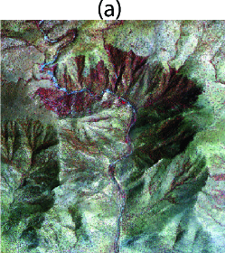
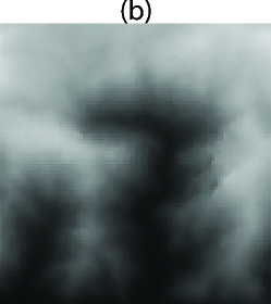
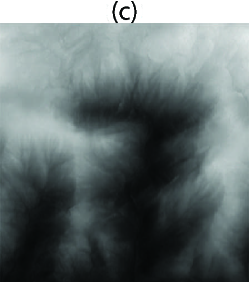
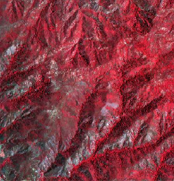


The Digital Elevation Model (DEM) is a digital representation of any three-dimensional surface. It is immensely useful in precision satellite data processing, geographic information systems [41], hydrological studies [29], urban planning [34], and many other key applications. The major sources of DEM generation are terrestrial, airborne, or space-borne, depending upon the platform used for data acquisition. However, each of these scenarios has its own set of advantages and disadvantages. While elevation models generated using terrestrial and airborne systems have high spatial resolution, their coverage is quite restricted and they typically suffer from several issues and systematic errors [14] [32]. Space-borne missions such as SRTM, and ASTER [13, 1], on the other hand, have almost global coverage but lack the resolution capability at the finest level. Due to the emerging significance and diverse applications of DEM, both its accuracy and resolution have a substantial impact in different fields of operation [39, 27]. However, high-resolution DEM products are expensive, as they require special acquisition and processing techniques to achieve desired results. As an alternative to generating high-resolution DEM from scratch, enhancing the resolution (super-resolution) of existing elevation datasets can be seen as the most optimal strategy to address the shortfall. Hence, we intend to take a step in this direction to generate high-resolution DEM and, to make it more tractable, we formulate this problem in an image super-resolution setting. As shown in Figure 1, our primary objective is to synthesize high-resolution DEM provided its coarser resolution and existing False Colour Composite (FCC) of high-resolution MX imagery.
Recent advances in deep neural networks and optimization techniques show compelling progress over conventionally driven approaches for various computer vision applications like image or video super-resolution. However, we found that very few methods approach the problem of DEM super-resolution, especially, for real-world datasets. We propose a novel framework, which effectively addresses this problem. Our key contributions can be summarized as follows -
-
1.
We propose a novel architecture for DEM super-resolution which effectively utilizes information from a high-resolution MX image as prior by conditioning it with a discriminative spatial self-attention.
-
2.
We develop and demonstrate SIRAN, a framework based on Sinkhorn regularized adversarial learning. We provide theoretical and empirical justification for its effectiveness in resolving the vanishing gradient issue while leveraging tighter iteration complexity.
-
3.
We generate our own dataset by using realistic coarse resolution data instead of bicubic downsampled.
-
4.
Finally, we perform experiments to assess the accuracy of our model along with ablation studies to study the impact of the different configuration choices.
In the following section, we briefly discuss recent works attempting to address similar problem.
2 Related Work
Super-resolution is one of the emerging research fields in the area of computer vision, especially SISR. Interpolation-based techniques like linear, and bicubic are widely used, but they under-perform at high frequency regions producing smoothed outputs [21]. To preserve edge information, multiple reconstruction-based methods like steering kernel regression (SKR) [40] or non-local means (NLM) [35], have also been proposed. Though they can fulfill their primary objective, they cannot produce super-resolved images at a large magnification factor.
DEM is an essential component in remote sensing applications, but research on DEM super-resolution is still limited. Xu et al. [45] proposed a super-resolution algorithm based upon NLM. However, after SISR attained the peak of its popularity with the first introduction of Super-resolution using Convolutional Neural Network (SRCNN) [10], its variant D-SRCNN was proposed by [6] to address the DEM super-resolution problem. It performs better than the non-local-based method. Xu et al. [46] brings in the concept of transfer learning where an EDSR (Enhanced Deep Super-Resolution Network) [30], pre-trained over natural images, is taken to obtain a high-resolution gradient map which is fine-tuned to generate high-resolution DEM. After the introduction of Generative Adversarial Network (GAN) by Goodfellow et al. [18] a substantial number of methods have evolved in the field of super-resolution like Super-resolution using GANs (SRGAN) [28]. Based on this recently, Benkir et al.[8] proposed a DEM super-resolution model, namely D-SRGAN, and later they suggested another model based on EffecientNetV2 [9] for DEM SISR. According to their claim, their proposed methods can outperform the previously mentioned studies in terms of DEM super-resolution.
However, GANs suffer from major issues of mode collapse and vanishing gradients despite providing realistic outcomes. To resolve this, Wasserstein GAN (WGAN) [2] and other variants [20] have been introduced. However, these methods are computationally expensive, which can be untangled by introducing an entropic regularization term [7] resulting in favorable sample complexity [17]. In this study, we explore the efficacy of sinkhorn distance [16] in DEM super-resolution, which is one of the forms of entropic optimal transport.
Guided super-resolution is a prominent research area in computer vision especially in the domain of depth estimation. One of the pioneering works in this domain is [26], where Kim et al. proposed Deformable Kernel Networks (DKN) and Faster DKN (FDKN) which learn sparse and spatially invariant filter kernels. Later, He et al. [23] exerts a high-frequency guided module to embed the guide details in the depth map. Recently, Metzger et al. [33] achieved state-of-the-art performance by adapting the concept of guided anisotropic diffusion with deep convolutional networks. Our proposed method can also be regarded in a similar group where our major attention is to introduce significant features from MX imagery to super-resolved DEM. In the following section, we discuss our overall framework.
3 Methodology
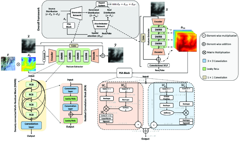
In Figure 2, we have illustrated a detailed architectural overview of our adversarial learning setup. The generator operates on upsampled coarser resolution DEM , MX image prior , consisting FCC of (R), (G) and (B) bands, and PSA of discriminator spatial feature maps, as conditional input. Let , where with being the joint distribution of FCC composition and , where constitute of upsampled coarser resolution DEM with . Let , where , where denotes the element-wise multiplication and denotes the generator distribution parameterized by . Let with represents the target high resolution DEM distribution. The discriminator classifies and to be coming from real or fake sample space and is assumed to be parameterized by .
3.1 Network Architecture
We design both and models based on ResNet [22] and DenseNet [25]. By combining the idea of skip and dense connections, respectively, we design a building block, namely a Densely connected Multi-Residual Block (DMRB), for our overall framework. Each DMRB block is constituted of multiple densely connected Residual Convolution Block (RCB). DMRB enables efficient context propagation and also stable gradient flow throughout the network. We endorse not using batch normalization as it degrades the performance and gives sub-optimal results for image super-resolution [43] scenarios. We kept the overall design of discriminator with a similar configuration as with an encoder followed by six DMRBs and finally a decoder to unravel the generated samples properly. The discriminator also adds a Multi-Layer Perceptron (MLP) layer to map its latent features into to required shape. Another reason behind the design of is to extract dense discriminative latent space features, which are passed as conditional input to the generator. In the following subsection, we will briefly explain this module.
3.1.1 Discriminator Spatial Attention
The feature maps from the latent space of the discriminator can be viewed as spatial attention to the generator. Since, the discriminator performs binary classification for a given input, apparently, in latent space, it captures the discriminative features that will help the generator to focus on salient parts of the input images. In [12], the authors introduced this concept of transferring domain-specific latent knowledge of discriminator as spatial attention to the generator. We use this information to condition the prior to focus on explicit features only.
Therefore, besides classification, has another major functional branch, , to approximate the spatial attention maps. For any input , is used to estimate its corresponding normalized spatial feature maps, . Let consists of DMRBs and be the activation maps after DMRB with output channels, such that . Since at different depths, the discriminator focuses on different features, we select different attention maps from the layers in the latent space. Eventually, attention coefficients are calculated as in [12]:
| (1) |
We use upsampled coarse resolution DEM to estimate these attention maps. This choice is motivated by the fact that unlike image-to-image translation in [12], during the test phase, we do not have high-resolution samples in the target domain. For this reason, we use the concept of domain adaptation loss from [38]. These attention maps are passed through a polarized self-attention (PSA) [31] block to exclude redundant features while highlighting significant areas. It is chosen because of its capability to retain the highest internal resolution [31] compared to other self-attention modules. The following section will describe the theoretical framework for optimizing our model.
3.2 Theoretical framework
The overall adversarial framework demonstrated in Figure 2 is trained by optimizing the minmax objective function of a conventional GAN between and ,
| (2) |
Despite stability issues, we stick with the conventional GAN objective function as in equation 2 due to its ease of implementation and less computational complexity compared to WGANs [2, 20]. In the following subsections, we define the objective function used for training.
3.2.1 Discriminator Objective Function
The objective function of in our framework is designed according to equation 2. In addition, we include domain adaptation loss [38] to enforce the discriminator model to mimic the latent features of the high-resolution data and sharpen spatial attention maps provided an upsampled low-resolution data. This loss is defined as
| (3) |
After incorporating domain adaptation loss with adversarial layout, the final objective function of becomes
| (4) |
where is the assigned weight for domain adaptation loss in the discriminator loss function.
3.2.2 Generator Objective Function
Apart from the adversarial loss , the objective function of is regularized with pixel loss and SSIM loss to associate to generate samples close to the ground truth. The ensures minimizing the pixel-wise differences while helps in preserving the perceptual quality and structural information between the predicted and ground truth images. Although, DEMs have almost no textures, accounts for crucial structural elements like variations in terrain height and slope, and also aids in capturing perceptually significant variations even in minimal texture scenarios to ensure a high-quality representation. These losses are defined below assuming .
| (5) | ||||
The key concern of utilizing an adversarial objective is the vanishing gradient problem near the optimal point. This leads to converge to a sub-optimal solution and results in a partially aligned generated distribution with respect to the true distribution. To avoid this, we regularize the generator objective by a distance metric between the generated and target distributions based on the concept of Entropic Optimal Transport (EOT).
Let and be the measure of generated and true distribution with support included in a compact bounded set , respectively. Therefore, the EOT [4] between the said measures can be defined using Kantarovich formulation as shown in equation 3.2.2 where we assume .
| (6) |
where, is the set of all joint distribution on having marginals and , is the cost of transferring unit mass between locations and , and the regularization term is the mutual information between two distribution measures [15] with being its weight factor. When the cost is chosen as a distance-metric the solution of equation 3.2.2 is referred to as entropic Wasserstein distance between two probability measures. The main reason behind considering EOT is due to its favorable sample complexity of [17], given a sample size , compared to [44] for OT which is the baseline principle of [2, 20].
To fit the generated measure to the true measure , we have to minimize the entropic Wasserstein distance between them and this can be treated as an objective function for the generator [3]. However, it has one major issue of being strictly larger than zero even if and are exactly aligned, i.e. . This is resolved by adding normalizing terms to equation 3.2.2, which leads to the Sinkhorn loss [16] as defined below.
| (7) |
Based on the value of , equation 7 shows asymptotic behaviour [16]. When , it recovers the conventional OT problem, while , it converges to maximum mean discrepency (MMD) [19]. Therefore, the Sinkhorn loss interpolates between OT loss and MMD loss as varies from to . Therefore, by properly tuning we can leverage the concurrent advantage of non-flat geometric properties of OT loss and, high dimensional rigidity and energy distance properties of MMD loss (when with ) by only utilizing Sinkhorn loss. Apart from this, the selection of also affects the overall gradients of , which eventually results in preventing vanishing gradient problems near the optimal point. This claim can be established from the smoothness property of with respect to . In this context, we propose Theorem 1, where we derive a formulation to estimate the smoothness of Sinkhorn loss.
Theorem 1 (Smoothness of Sinkhorn loss).
Consider the Sinkhorn loss between two measures and on and two bounded subsets of , with a , -Lipschitz, and -smooth cost function . Then, for , one has,
| (8) | ||||
where is the Lipschitz in corresponding to , , with amd being the minimum and maximum values in set . Let represent the smoothness mentioned above, then we get the following asymptotic behavior in :
-
1.
as ,
-
2.
as ,
Proof.
Refer to Appendix A. ∎
Theorem 1 shows the variation of smoothness of with respect to . Using this, we can estimate the upper bound of the overall expected gradient of our proposed adversarial set-up. Hence, to formulate this upper bound, we present Proposition 1.
Proposition 1.
Let , and be the objective functions related to supervised losses, adversarial loss and Sinkhorn loss respectively, and and be the parameters of optimal generator and discriminator . Let us suppose , where , is -smooth in . If and , then , where is the derived smoothness of Sinkhorn loss in equation 8.
Proof.
Refer to Appendix B. ∎
In a traditional adversarial set-up as mentioned in [37], suggests reductions of , which eventually results in a vanishing gradient near the optimal region. However, in our Sinkhorn regularized adversarial framework, the upper bound is also dependent on as exhibited in Proposition 1. From equation 8, is exponentially variable with respect to the choice of . Hence, the selection of adequate will have a profound impact in mitigating the vanishing gradient problem suffered by regular adversarial setup.
Apart from resolving the vanishing gradient problem, our Sinkhorn regularized adversarial set-up leads to faster numerical convergence of the supervised loss resulting in more stringent iteration complexity [37]. Therefore, we present Proposition 2 to deduce the iteration complexity of our proposed adversarial framework.
Proposition 2.
Suppose the supervised loss is lower bounded by and it is twice differentiable. For some arbitrarily small , and stationary point with , let , and , with conditions , and , then the iteration complexity in Sinkhorn regularized adversarial framework is upper bounded by , assuming .
Proof.
Refer to Appendix C. ∎
Corollary 1.
Using first order Taylor series, the upper bound in Proposition 2 becomes .
Proof.
Refer to Appendix C.1. ∎
Since the denominator of the derived upper bound in Proposition 2 is greater than the one mentioned in Theorem 3 of [37], we can infer that our proposed learning framework has tighter iteration complexity compared to the general adversarial setup. This is only true when , and it can be easily satisfied by appropriate choice of . It can also be verified using a simpler setup as shown in Corollary 1, as it increases the convergence rate from [37] to which effects considerably in the training iterations as shown in section 5.3 as well as in appendix D. This also suggests that our setup is equivalent to applying two discriminator operations without involving additional computations which helps in effectively leveraging the advantage of using multiple discriminators [11]. Due to lack of space, experiment results to support the proposed theorem and propositions are carried out in Appendix D.
Due to the mentioned advantages, we have regularized the overall generator loss with Sinkhorn distance which is defined below assuming .
| (9) |
where and represent the measure of generated and true distributions, respectively. is estimated according to [16] which utilizes and the Sinkhorn iterations as the major parameters. Therefore, the overall generator loss can be defined as,
| (10) |
where , , and represent the weight assigned to pixel loss, SSIM loss, adversarial loss, and Sinkorn loss respectively.
4 Experiments

In this section, we discuss experiments to analyze the efficacy of our proposed model in DEM super-resolution.
4.1 Datasets
DEM super-resolution is a relatively unexplored area that suffers from a lack of realistic datasets. Therefore, in this study, we generate our own DEM super-resolution dataset. From the real-world application point of view, we leverage to use real coarse resolution SRTM DEM with a ground sampling distance (GSD) of 30m as input instead of conventional bicubic downsampled while taking Indian high-resolution DEM (GSD=10m) generated from Cartosat-1 stereoscopic satellite, as the ground truth. For the image prior, we utilize the high-resolution MX data (GSD=1.6m) from the Cartosat-2S satellite. The DEMs are upsampled to the resolution of MX images using bicubic interpolation to generate a paired dataset. This helps in increasing the training samples as well as assists the model to learn dense high-resolution features from the prior. The dataset consists of 72,000 patches of size , which includes various signatures such as vegetation, mountains, and, water regions. We use 40,000 samples for training, 20,000 for cross-validation, and 12,000 for testing, where 10,000 patches belong to the Indian subcontinent region and the rest outside India. As ground truth DEM data is only available for Indian regions, our model is trained on limited landscape areas. To check its generalization capability, we also test our model on data from outside India from the Fallbrook region, US, where Cartosat DEM data is unavailable. For these cases, we validate our result based on available 10m DEM data of the 3D Elevation Program (3DEP) [42].
4.2 Implementation Details
All the experiments are conducted under identical environments. We use convolution kernel and leaky ReLU activation except in global skip connection where kernel is used without any activation. Each DMRB has 64 convolution operations. We use ADAM optimizer with a fixed learning rate of 0.0001. During adversarial training, we update the critic once every single update in the generator. We set , , , and . For estimating , we set and . The entire framework is developed using PyTorch. All the experiments are performed on 2 Nvidia V100 GPUs. During testing, our model takes 0.46s for a single patch in one GPU.
5 Result Analysis
In this section, we analyze both qualitatively and quantitatively, the quality of our proposed super-resolved DEMs. We compare it with traditional bicubic as well as other learning-based state-of-the-art methods [8, 9] which also includes recent baseline models for image-guided depth super-resolution [26, 33, 23].
| Method | RMSE (m) | MAE (m) | SSIM(%) | PSNR | ||||
|---|---|---|---|---|---|---|---|---|
| Dataset | Inside | Outside | Inside | Outside | Inside | Outside | Inside | Outside |
| Bicubic | 15.25 | 23.19 | 12.42 | 22.04 | 71.27 | 66.49 | 30.07 | 27.79 |
| ENetV2 [9] | 20.35 | 30.53 | 18.72 | 28.36 | 69.63 | 60.04 | 31.74 | 25.58 |
| DKN [26] | 12.89 | 21.16 | 11.18 | 19.78 | 73.59 | 68.45 | 32.09 | 28.22 |
| FDKN [26] | 13.05 | 21.93 | 11.34 | 20.41 | 74.13 | 66.83 | 32.46 | 27.68 |
| DADA [33] | 37.49 | 40.89 | 32.17 | 37.74 | 73.32 | 69.86 | 27.94 | 26.78 |
| ESRGAN [8] | 31.33 | 20.45 | 25.56 | 18.34 | 82.48 | 75.67 | 29.88 | 29.05 |
| FDSR [23] | 12.98 | 30.58 | 10.87 | 25.28 | 81.49 | 59.81 | 33.77 | 25.59 |
| SIRAN (ours) | 9.28 | 15.74 | 8.51 | 12.25 | 90.59 | 83.90 | 35.06 | 31.56 |
5.1 Quantitative Analysis
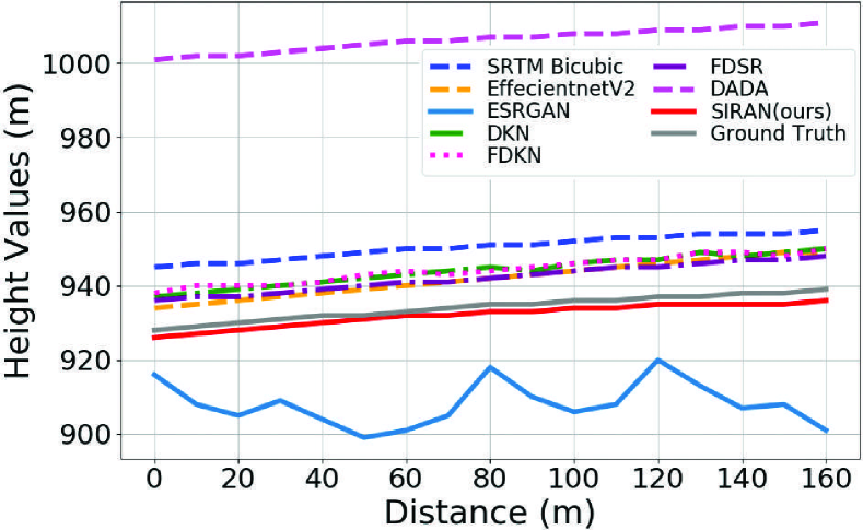
To quantitatively analyze the outcomes of DEM super-resolution, we use RMSE, MAE, PSNR, and SSIM as evaluation metrics. Our proposed method outperforms other state-of-the-art methods, as illustrated in Table 1. For both inside and outside India patches, our method not only retains the elevation values but also captures high-resolution structural details with fidelity. This results in more than 24% improvement in RMSE and MAE, 8% in SSIM, and 4% in PSNR with respect to the second best in each criterion. Despite having different source domains for reference DEM for patches outside India, our method performs substantially in generating high-resolution DEM as depicted in the above table which suggests better generalization capability of our model compared to others. Among the other methods, FDSR [23] performs closely to our model for Indian patches. However, for outside patches, its performance deteriorates. Although ESRGAN captures the high structural details, it has poor RMSE and MAE due to the presence of noise. In Figure 5, we have demonstrated the line profile analysis of SIRAN as well as other baseline models with respect to the ground truth. Compared to others, SIRAN not only has the lowest bias but also follows the true elevation values most closely. This supports the error analysis in Table 1.
5.2 Qualitative Analysis
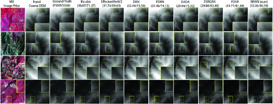
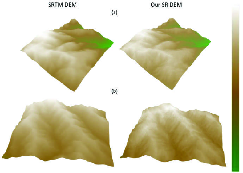
Figure 3 demonstrates the qualitative analysis of our proposed method for patches of India. Compared to other approaches, SIRAN is able to highlight key features and retain the perceptual quality with respect to ground truth. ESRGAN also captures substantial structural information in its outcomes, however, it tends to produce artifacts and noise in the generated DEM which is depicted in Table 1 and Figure 5. In Figure 4, we have compared the outcomes for patches from outside India. As indicated before, compared to other baseline techniques, our method is able to generate higher resolution DEM in close proximity to the reference DEM despite having a different source domain. Although FDSR [23] performed well for Indian patches, due to lack of generalization capability it introduces image details more prominently in the generated DEM for test patches outside India. In Figure 6, we demonstrate 3-D visualization of generated DEMs, corresponding to a region, where ground truth is unavailable. We compare it with available SRTM DEM, and clearly, our topographic view of generated DEM captures sharper features in mountainous regions as well as in the tributaries of the water basin area as shown in Figure 6.
|
|
PSA |
|
RMSE (m) | MAE (m) | SSIM (%) | PSNR | ||||||
|---|---|---|---|---|---|---|---|---|---|---|---|---|---|
| ✗ | ✗ | ✗ | ✗ | 16.54 | 13.63 | 72.27 | 30.25 | ||||||
| ✓ | ✗ | ✗ | ✗ | 29.32 | 25.41 | 78.29 | 28.25 | ||||||
| ✓ | ✓ | ✗ | ✗ | 20.76 | 18.29 | 81.68 | 31.08 | ||||||
| ✓ | ✓ | ✓ | ✗ | 18.76 | 15.13 | 85.04 | 32.21 | ||||||
| ✓ | ✓ | ✓ | ✓ | 9.28 | 8.51 | 90.49 | 35.06 |
5.3 Ablation Study
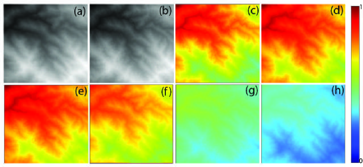
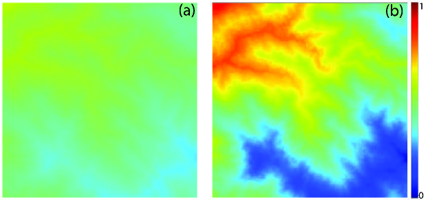
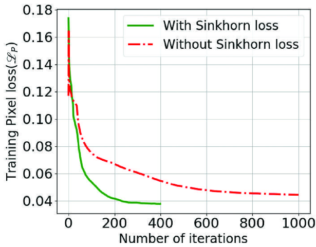
In this section, we analyze the efficacy of our four proposed modules, image prior, spatial attention from discriminator, PSA, and Sinkhorn loss-based adversarial learning. In the absence of any prior, it leads to outcomes similar to bicubic interpolation that affects its SSIM score as shown in Table 2. Using high-resolution MX image priors resolves this issue to a certain extent by increasing SSIM by more than 6%. Yet, this degrades the performance of the model in terms of RMSE and MAE. To improve upon this situation, we introduce spatial feature maps from the discriminator. Figure 7 shows how individual attention maps after each DMRB prioritizes certain features at different labels. However, the mean attention weights are approximately uniform as shown in Figure 8. PSA handles this matter by emphasizing key features. Addressing both these attentions improves the RMSE and MAE by more than 50% as well as enhances SSIM by almost 7% as shown in Table 2. The introduction of Sinkhorn distance regularization enhances the evaluation parameters further with both MAE and RMSE below 10 m and SSIM more than 90% as shown in Table 2. Apart from this, sinkhorn loss also contributed to a near 2.5X faster convergence rate for the pixel loss as shown in Figure 9. This also supports our argument in Proposition 2.
6 Conclusions
In this paper, we demonstrated an effective approach for DEM super-resolution using realistic coarse data samples. Unlike regular SISR, the method uses high-resolution MX images as prior in a specially designed architectural framework consisting of spatial attention maps from discriminator, PSA, and DMRBs, optimized using Sinkhorn distance regularized adversarial learning. We provided theoretical and empirical evidence to show how this choice stabilizes the training of our adversarial model and improves its convergence. We perform quantitative and qualitative analysis by generating and comparing DEMs related to different signatures along with investigating generalization capability by testing out-of-domain samples. We also analyse how each proposed module affects the outcomes. Our method achieves favorable results compared to other state-of-the-art methods. In the future, we would like to investigate the effect of Sinkhorn loss on sub-optimality gap and generalization error.
References
- Abrams et al. [2020] Michael Abrams, Robert Crippen, and Hiroyuki Fujisada. Aster global digital elevation model (gdem) and aster global water body dataset (astwbd). Remote Sensing, 12(7), 2020.
- Arjovsky et al. [2017a] Martin Arjovsky, Soumith Chintala, and Léon Bottou. Wasserstein generative adversarial networks. In Proceedings of the 34th International Conference on Machine Learning, pages 214–223. PMLR, 2017a.
- Arjovsky et al. [2017b] Martin Arjovsky, Soumith Chintala, and Léon Bottou. Wasserstein gan, 2017b.
- Aude et al. [2016a] Genevay Aude, Marco Cuturi, Gabriel Peyré, and Francis Bach. Stochastic optimization for large-scale optimal transport, 2016a.
- Aude et al. [2016b] Genevay Aude, Marco Cuturi, Gabriel Peyré, and Francis Bach. Stochastic optimization for large-scale optimal transport, 2016b.
- Chen et al. [2016] Zixuan Chen, Xuewen Wang, Zekai Xu, and Hou Wenguang. Convolutional neural network based dem super resolution. ISPRS - International Archives of the Photogrammetry, Remote Sensing and Spatial Information Sciences, XLI-B3:247–250, 2016.
- Cuturi [2013] Marco Cuturi. Sinkhorn distances: Lightspeed computation of optimal transportation distances. Advances in Neural Information Processing Systems, 26, 2013.
- Demiray et al. [2020] Bekir Z. Demiray, Muhammed Ali Sit, and Ibrahim Demir. D-SRGAN: DEM super-resolution with generative adversarial networks. CoRR, abs/2004.04788, 2020.
- Demiray et al. [2021] Bekir Z Demiray, Muhammed Sit, and Ibrahim Demir. Dem super-resolution with efficientnetv2, 2021.
- Dong et al. [2014] Chao Dong, Chen Change Loy, Kaiming He, and Xiaoou Tang. Image super-resolution using deep convolutional networks. IEEE Transactions on Pattern Analysis and Machine Intelligence, 38, 2014.
- Durugkar et al. [2016] Ishan P. Durugkar, Ian Gemp, and Sridhar Mahadevan. Generative multi-adversarial networks. CoRR, abs/1611.01673, 2016.
- Emami et al. [2019] Hajar Emami, Majid Moradi Aliabadi, Ming Dong, and Ratna Babu Chinnam. SPA-GAN: spatial attention GAN for image-to-image translation. CoRR, abs/1908.06616, 2019.
- Farr and Kobrick [2000] T. G. Farr and M. Kobrick. Shuttle radar topography mission produces a wealth of data. Eos Trans. AGU, 81:583-583, 2000.
- Fisher and Tate [2006] Peter Fisher and Nicholas Tate. Causes and consequences of error in digital elevation models. progress in physical geography. Progress in Physical Geography, 30, 2006.
- Genevay et al. [2016] Aude Genevay, Marco Cuturi, Gabriel Peyré, and Francis R. Bach. Stochastic optimization for large-scale optimal transport. ArXiv, abs/1605.08527, 2016.
- Genevay et al. [2018] Aude Genevay, Gabriel Peyre, and Marco Cuturi. Learning generative models with sinkhorn divergences. In Proceedings of the Twenty-First International Conference on Artificial Intelligence and Statistics, pages 1608–1617. PMLR, 2018.
- Genevay et al. [2019] Aude Genevay, Lénaic Chizat, Francis Bach, Marco Cuturi, and Gabriel Peyré. Sample complexity of sinkhorn divergences, 2019.
- Goodfellow et al. [2014] Ian Goodfellow, Jean Pouget-Abadie, Mehdi Mirza, Bing Xu, David Warde-Farley, Sherjil Ozair, Aaron Courville, and Yoshua Bengio. Generative adversarial nets. In Advances in Neural Information Processing Systems. Curran Associates, Inc., 2014.
- Gretton et al. [2008] Arthur Gretton, Karsten M. Borgwardt, Malte J. Rasch, Bernhard Schölkopf, and Alexander J. Smola. A kernel method for the two-sample problem. CoRR, abs/0805.2368, 2008.
- Gulrajani et al. [2017] Ishaan Gulrajani, Faruk Ahmed, Martín Arjovsky, Vincent Dumoulin, and Aaron C. Courville. Improved training of wasserstein gans. CoRR, abs/1704.00028, 2017.
- He and Siu [2011] He He and Wan-Chi Siu. Single image super-resolution using gaussian process regression. In CVPR 2011, pages 449–456, 2011.
- He et al. [2015] Kaiming He, Xiangyu Zhang, Shaoqing Ren, and Jian Sun. Deep residual learning for image recognition. CoRR, abs/1512.03385, 2015.
- He et al. [2021] Lingzhi He, Hongguang Zhu, Feng Li, Huihui Bai, Runmin Cong, Chunjie Zhang, Chunyu Lin, Meiqin Liu, and Yao Zhao. Towards fast and accurate real-world depth super-resolution: Benchmark dataset and baseline. 2021 IEEE/CVF Conference on Computer Vision and Pattern Recognition (CVPR), pages 9225–9234, 2021.
- Houdard et al. [2021] Antoine Houdard, Arthur Leclaire, Nicolas Papadakis, and Julien Rabin. On the existence of optimal transport gradient for learning generative models, 2021.
- Huang et al. [2016] Gao Huang, Zhuang Liu, and Kilian Q. Weinberger. Densely connected convolutional networks. CoRR, abs/1608.06993, 2016.
- Kim et al. [2021] Beomjun Kim, Jean Ponce, and Bumsub Ham. Deformable kernel networks for joint image filtering. International Journal of Computer Vision, 129, 2021.
- Kim et al. [2019] Dong-Eon Kim, Philippe Gourbesville, and Shie-Yui Liong. Overcoming data scarcity in flood hazard assessment using remote sensing and artificial neural network. Smart Water, 4:1–15, 2019.
- Ledig et al. [2017] Christian Ledig, Lucas Theis, Ferenc Huszár, Jose Caballero, Andrew Cunningham, Alejandro Acosta, Andrew Aitken, Alykhan Tejani, Johannes Totz, Zehan Wang, and Wenzhe Shi. Photo-realistic single image super-resolution using a generative adversarial network. In 2017 IEEE Conference on Computer Vision and Pattern Recognition (CVPR), pages 105–114, 2017.
- Li and Wong [2010] Jing Li and David Wong. Effect of dem sources on hydrologic applications. Computers, Environment and Urban Systems, 34:251–261, 2010.
- Lim et al. [2017] Bee Lim, Sanghyun Son, Heewon Kim, Seungjun Nah, and Kyoung Mu Lee. Enhanced deep residual networks for single image super-resolution. CoRR, abs/1707.02921, 2017.
- Liu et al. [2021] Huajun Liu, Fuqiang Liu, Xinyi Fan, and Dong Huang. Polarized self-attention: Towards high-quality pixel-wise regression. CoRR, abs/2107.00782, 2021.
- Liu [2008] Xiaoye Liu. Airborne lidar for dem generation: Some critical issues. progress in physical geography. Progress in Physical Geography - PROG PHYS GEOG, 32:31–49, 2008.
- Metzger et al. [2023] Nando Metzger, Rodrigo Caye Daudt, and Konrad Schindler. Guided depth super-resolution by deep anisotropic diffusion. 2023 IEEE/CVF Conference on Computer Vision and Pattern Recognition (CVPR), 2023.
- Priestnall et al. [2000] Gary Priestnall, Jad Jaafar, and A. Duncan. Extracting urban features from lidar digital surface models. Computers, Environment and Urban Systems, 24:65–78, 2000.
- Protter et al. [2009] Matan Protter, Michael Elad, Hiroyuki Takeda, and Peyman Milanfar. Generalizing the nonlocal-means to super-resolution reconstruction. IEEE Transactions on Image Processing, 18(1):36–51, 2009.
- Radford et al. [2015] Alec Radford, Luke Metz, and Soumith Chintala. Unsupervised representation learning with deep convolutional generative adversarial networks. CoRR, abs/1511.06434, 2015.
- Rout [2020] Litu Rout. Understanding the role of adversarial regularization in supervised learning. CoRR, abs/2010.00522, 2020.
- Rout et al. [2020] Litu Rout, Indranil Misra, S Manthira Moorthi, and Debajyoti Dhar. S2a: Wasserstein gan with spatio-spectral laplacian attention for multi-spectral band synthesis, 2020.
- Sørensen and Seibert [2007] Rasmus Sørensen and Jan Seibert. Effects of dem resolution on the calculation of topographical indices: Twi and its components. Journal of Hydrology, 347:79–89, 2007.
- Takeda et al. [2007] Hiroyuki Takeda, Sina Farsiu, and Peyman Milanfar. Kernel regression for image processing and reconstruction. IEEE Transactions on Image Processing, 16(2):349–366, 2007.
- Trevisani et al. [2012] Sebastiano Trevisani, Marco Cavalli, and Lorenzo Marchi. Surface texture analysis of a high-resolution dtm: Interpreting an alpine basin. Geomorphology, s 161–162:26–39, 2012.
- [42] U.S. Geological Survey (USGS). 1/3rd arc-second digital elevation models (dems)- usgs national map 3dep downloadable data collection. 2019.
- Wang et al. [2018] Yifan Wang, Federico Perazzi, Brian McWilliams, Alexander Sorkine-Hornung, Olga Sorkine-Hornung, and Christopher Schroers. A fully progressive approach to single-image super-resolution. CoRR, abs/1804.02900, 2018.
- Weed and Bach [2017] Jonathan Weed and Francis Bach. Sharp asymptotic and finite-sample rates of convergence of empirical measures in wasserstein distance, 2017.
- Xu et al. [2015] Zekai Xu, Xuewen Wang, Zixuan Chen, Xiong Dongping, Mingyue Ding, and Hou Wenguang. Nonlocal similarity based dem super resolution. ISPRS Journal of Photogrammetry and Remote Sensing, 110:48–54, 2015.
- Xu et al. [2019] Zekai Xu, Zixuan Chen, Weiwei Yi, Qiuling Gui, Hou Wenguang, and Mingyue Ding. Deep gradient prior network for dem super-resolution: Transfer learning from image to dem. ISPRS Journal of Photogrammetry and Remote Sensing, 150:80–90, 2019.
Supplementary Material
A Proof of Theorem 1: Smoothness of Sinkhorn Loss
We will define some of the terminologies, which are necessary for this proof. From equation 6 of the main paper, the entropic optimal transport can be defined as, ()
| (11) |
where we assume such that . The formulation in equation A corresponds to the primal problem of regularized OT and, this allows us to express the dual formulation of regularized OT as the maximization of an expectation problem, as shown in equation 12 [5].
| (12) | ||||
where is set of real valued continuous functions for domain and and they are referred as dual potentials. Now, given optimal dual potentials , and , the optmal coupling as per [5] can be defined as
| (13) |
To prove Theorem 2, we need an important property regarding its Lipschitz continuity of the dual potentials, which is explained in the following Lemma.
Lemma A.1.
If is Lipschitz, then the dual potentials are also Lipschitz.
Proof.
As , is -Lipschitz in . As, the entropy is selected as Shannon entropy, according to [7] using the softmin operator, the optimal potential satisfy the following equation
| (14) |
Now, to estimate the Lipschitz of , we have to find the upper bound of . Hence, taking the gradient of equation 4 with respect to and its norm,
| (15) |
Now due to Lipschitz continuity of , we can say . Hence, using Cauchy-Schwarz inequality we will get,
| (16) | ||||
| (17) |
This completes the proof of the lemma. An alternative proof is provided in [24] in Proposition 4. Similarly, it can be proved for the other potential term. ∎
For any , will result in different coupling solutions , for . Now, based on Danskins’ theorem for optimal coupling , we can write
| (18) |
Therefore, for any and , we can write,
| (19) |
Now with respect to different , for with different pair of dual potentials, the can be written as below. For simplicity we denote , , , and .
| (20) |
From [17], we know, as the dual potentials are -Lipschitz, , we can write, . And from property of c-transform, for we can also write . We assume to be a bounded set in our case, hence, denoting as the diameter of the space, at optimality, we can get that
| (21) |
Hence, the exponential terms in equation 20 are bounded, and we can assume it has a finite Lipschitz constant . Taking , and using Cauchy-Schwarz, we can rewrite equation 20 as,
| (22) |
Now, as the input space and output space are bounded, the corresponding measures and will also be bounded. We assume, and . If we apply equation 21 in equation 13, to get the upper bound of the coupling function, we will get which is less than the bound in equation 22. Then, we can find some constant upper bound of , using the assumed bounds of measures and can write , such that,
| (23) | ||||
Then using the marginal condition as shown in equation A, we can write equation 22 as,
| (24) |
The input set is a compact set such that . So, assuming and to be the minimum and maximum value in set and considering the whole situation in discrete space, equation 24 can be rewritten as,
| (25) |
Now, taking , and doing necessary subtraction and division on both sides of equation 25, it can be rewritten as
| (26) |
Equation 26 satisfies because . As, , from equation 26, it can be written as
| (27) |
Substituting equation 27 in equation A, we will get,
| (28) |
So, the EOT problem defined in equation A has smoothness in with . From this, we can derive the smoothness of Sinkhorn loss defined in equation 7 of the main paper. Note that only the first two terms in equation 7 of the main paper are dependent. Therefore, they only contribute to the gradient approximation and both of them will satisfy the same smoothness condition as defined in equation A. So, if sinkhorn loss has smoothness , it will satisfy, . In general, we can define the smoothness of sinkhorn loss with as,
| (29) |
This completes proof of the statement in Theorem 2
B Proof of Proposition1
This proof is inspired by [37]. Assuming be the smoothness in for Sinkhorn loss , where . For simplicity, we use a common set for inputs and outputs as . Hence, to approximate the gradient of sinkhorn loss, using Jensen’s inequality, we can write,
| (30) |
Say, for optimized parameter , . Since, , we can write using the smoothness of sinkhorn loss and Lipschitz of model parameters,
| (31) |
At optimal condition, as the distributions of and are aligned for optimal . So, by substituting equation B in equation B, we will get
| (32) |
From Lemma 1 of [37], we get,
| (33) |
Similarly, from Lemma 2 of [37], we get
| (34) |
Here, is parameters of discriminator . So using equations 32, 33, and 34, for the combination of losses we will get,
| (35) |
This completes the proof of Proposition 1.
C Proof of Proposition2
This proof also follows the steps of Theorem 3 from [37]. In the sinkhorn regularized adversarial setup, the parameters are updated using fixed step gradient descent. They iterate as,
| (36) |
For simplicity, we denote . Using Taylor’s expansion,
| (37) | ||||
Now, substituting from equation C, and using triangle inequality and Cauchy-Schwarz inequality, equation 37 can be rewritten as,
| (38) |
Taking into account the assumptions in Proposition 2 and utilizing Minkowski’s inequality, equation C can be rewritten as,
| (39) |
Using , from equation C, we can write,
| (40) |
Assuming T iterations to reach this -stationary point, then for , doing telescopic sum over ,
| (41) |
Therefore, using the iteration complexity definition of [37], we obtain,
| (42) | ||||
This completes the proof of Proposition 2.
C.1 Proof of Corollary1
Using the similar arguments of Proposition 2, and taking first-order Taylor’s approximation, we get
| (43) |
Taking telescopic sum over for , we get
| (44) |
So, using the definition of iteration complexity, we get,
| (45) | ||||
This completes the proof of Corollary 2.
D Experiments
We perform experiments to answer the proposed claims in our paper. There are two main aspects we want to investigate, firstly, how the choice of affects the overall training of the model, and secondly, how it performs compared to other state-of-the-art learning methods like WGAN, WGAN+GP, and DCGAN. In both these cases, we analyze the claims of mitigating vanishing gradients in the near-optimal region and fast convergence rate.
D.1 Implementation details
In this setting, we are performing a denoising operation on the MNIST dataset. For this 60000 samples of size are used during training, while 10000 are used for testing. The convergence criterion is set to be the mean square error of 0.04 or a maximum of 500 epochs. During training, we randomly add Gaussian noise to the training samples to perform the denoising task. The generator is designed as a simple autoencoder structure with an encoder and decoder each having 2 convolutional layers. In practice, we notice that a discriminator with shallow layers is usually sufficient to offer a higher convergence rate. Therefore, we choose, a three-layer fully connected network with 1024 and 256 hidden neurons. All the layers are followed by ReLu activation except the output layer. For optimization, ADAM is utilized with a learning rate of 0.001 with a batch size of 64, and the discriminator is updated once for every single update of the generator.
D.2 Results analysis
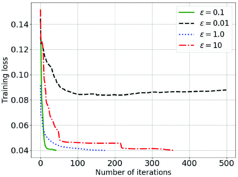
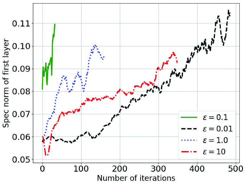
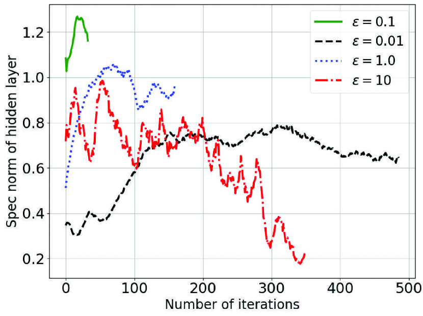
Figure 10, shows how changing the value of affects the overall iteration complexity. According to this figure, the instances are very small and very large, and the learning behavior of the model becomes close to regular adversarial setup which ultimately results in more time requirement for convergence. This is because, as and , the smoothness of sinkhorn loss tends to become independent of as depicted in Theorem 1, which makes the overall setup similar to the regular adversarial framework. This also affects the capability of mitigating the vanishing gradient problem as shown in Figure 2. The gradients are approximated using spectral norm and they are moving averaged for better visualization. From Figure 11(a), in the case of the first layer, as varies, the estimated gradients are similar near the optimal region. However, From Figure 11(b), we can see for the case of the hidden layer, gradient approximation is definitely affected by the choice of , and we can see as and , the gradients near-optimal region become smaller. However, using tends to have higher gradients even if near the optimal region. Therefore, this model will have more capability of mitigating the vanishing gradient problem. Hence, we use this model to compare with other benchmark methods.
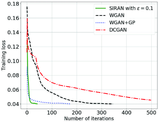
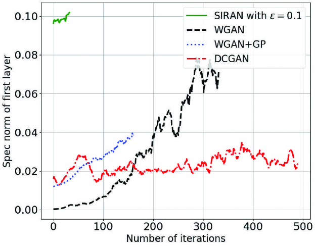
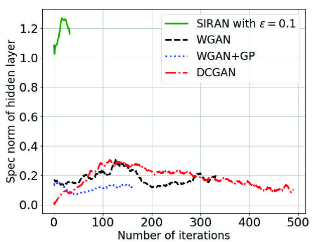
We compare the rate of convergence and capability of handling the vanishing gradient of SIRAN with WGAN [3], WGAN+GP [20], and DCGAN [36]. Figure 3 clearly visualizes how our proposed framework has tighter iteration complexity than others, and reaches the convergence faster. This is consistent with the theoretical analysis presented in Proposition 3. Figure 4, also provides empirical evidence of the vanishing gradient issue presented in Proposition 2. Both for the first layer and hidden layer, as shown in Figure 4, the approximated gradients are higher comparatively than others near the optimal region. This results in increasing the effectiveness of SIRAN in handling the issue of the vanishing gradient problem as discussed in Section 3.2.2 in the main paper.