An hp𝑝hp-Adaptive Sampling Algorithm on Dispersion Relation Reconstruction for 2D Photonic Crystals

Yueqi Wang  and  Guanglian Li Department of Mathematics, The University of Hong Kong, Pokfulam Road, Hong Kong. Email: u3007895@connect.hku.hk YW acknowledges support from the Research Grants Council (RGC) of Hong Kong via the Hong Kong PhD Fellowship Scheme (HKPFS).Department of Mathematics, The University of Hong Kong, Pokfulam Road, Hong Kong. Email: lotusli@maths.hku.hk GL acknowledges the support from Newton International Fellowships Alumni following-on funding awarded by The Royal Society, Young Scientists fund (Project number: 12101520) by NSFC and Early Career Scheme (Project number: 27301921), RGC, Hong Kong.
Abstract

Computing the dispersion relation for two-dimensional photonic crystals is a notoriously challenging task: It involves solving parameterized Helmholtz eigenvalue problems with high-contrast coefficients. To resolve the challenge, we propose a novel hp𝑝hp-adaptive sampling scheme that can detect singular points via adaptive mesh refinement in the parameter domain, and meanwhile, allow for adaptively enriching the local polynomial spaces on the elements that do not contain singular points. In this way, we obtain an element-wise interpolation on an adaptive mesh. We derive an exponential convergence rate when the number of singular points is finite, and a first-order convergence rate otherwise. Numerical tests are provided to illustrate its performance.
Key words: photonic crystals, band function reconstruction, adaptive mesh, element-wise interpolation

1 Introduction

This work is concerned with propagation of electromagnetic waves within photonic crystals (PhCs). PhCs are dielectric materials with a period size comparable to the wavelength [16]. The properties of waves in PhCs depend heavily on their frequencies, and for certain frequencies, they may be unable to propagate through PhCs, leading to the band gap phenomenon. This intriguing feature has led to the development of important applications, e.g., optical transistors, photonic fibers, and low-loss optical mirrors [36, 26, 33, 23]. We focus on two-dimensional (2D) PhCs, which are homogeneous along the z𝑧z axis and have high-contrast dielectric columns or holes in dielectric materials within the x𝑥x-y𝑦y plane.

The propagation of electromagnetic waves is governed by the Maxwell system. For 2D infinite crystals with perfect periodicity, Bloch theorem states that the problem is reduced to 2D parameterized Helmholtz eigenvalue problems defined over the unit cell with periodic boundary conditions. The associated parameter is the so-called wave vector 𝐤𝐤\mathbf{k}, which varies in the irreducible Brillouin zone (IBZ) [22]. The n𝑛nth band function ωnsubscript𝜔𝑛\omega_{n} (or the square root of the n𝑛nth largest eigenvalue up to a constant) is a function of the wave vector for all n+𝑛subscriptn\in\mathbb{N}_{+}. The band gap is the distance between two adjacent band functions. Thus, computing the n𝑛nth band function ωn(𝐤)subscript𝜔𝑛𝐤\omega_{n}(\mathbf{k}) involves solving infinite many Helmholtz eigenvalue problems defined on the unit cell. To obtain the band gap, it is necessary for the permittivity to take different values in the inclusion and background of the unit cell, and moreover, the ratio between these values, known as contrast, should be large. However, solving Helmholtz eigenvalue problems with high-contrast and piecewise constant coefficients poses significant challenges. Numerically, one possible approach is to limit the parameter 𝐤𝐤\mathbf{k} to a coarse mesh of the IBZ or even its edges only. However, it is inadequate for identifying small band gaps, e.g., avoided crossings, which are important in certain application areas of photonic materials. For example, it is important to avoid the smallest band gaps when manufacturing large-pitch photonic crystal fibers [9], whereas leakage channel fibers exploit the smallest band gaps [7]. While directly solving the eigenvalue problem over a very fine parametric discretization is failure-safe, it is highly inefficient. Band structure diagram paths based on crystallography categorize wave vectors by their symmetry and provide preferred band paths for band function reconstruction [14]. These important wave vectors are located at the face and edge centers, and vertices of Brillouin zone. However, there is no guaranteed accuracy.

The main goal of this paper is to provide a numerical method with guaranteed fast convergence rate. More specifically, let \mathcal{B} be the parameter domain, i.e., IBZ. Let ω(𝐤)C()𝜔𝐤𝐶\omega(\mathbf{k})\in C(\mathcal{B}) be a band function and Pn()subscript𝑃𝑛P_{n}(\mathcal{B}) the space of global polynomial functions of degree at most n𝑛n. The best approximation to ω(𝐤)𝜔𝐤\omega(\mathbf{k}) in Pn()subscript𝑃𝑛P_{n}(\mathcal{B}) with respect to the uniform norm ,\|\cdot\|_{\infty,\mathcal{B}} on \mathcal{B} can be measured by

En(ω):=infpPn()ωp,.assignsubscript𝐸𝑛𝜔subscriptinfimum𝑝subscript𝑃𝑛subscriptnorm𝜔𝑝E_{n}(\omega):=\inf_{p\in P_{n}(\mathcal{B})}\|\omega-p\|_{\infty,\mathcal{B}}.

If ωC1()𝜔superscript𝐶1\omega\notin C^{1}(\mathcal{B}), then En(ω)subscript𝐸𝑛𝜔E_{n}(\omega) cannot decay faster than first order with respect to n𝑛n, i.e., En(ω)=𝒪(n1)subscript𝐸𝑛𝜔𝒪superscript𝑛1E_{n}(\omega)=\mathcal{O}(n^{-1}) [31, Chapter 7]. Furthermore, this decay rate may not be improved in a subdomain where the band function is analytic [18]. The decay rate is only 𝒪(N1/2)𝒪superscript𝑁12\mathcal{O}(N^{-1/2}) in terms of the number N𝑁N of sampling points N𝑁N. In [34], we have developed a global polynomial interpolation method (GPI) to reconstruct the band function, focusing on selecting sampling points to achieve this slow convergence rate. Thus, there is an imperative need to develop more effective computational techniques for band structure reconstruction.

To improve the convergence of GPI, it is critical to exploit piecewise analyticity of band functions and to utilize local polynomial interpolation. This work focuses on adaptively selecting the wave vectors. Inspired by the hh, p𝑝p, and hp𝑝hp versions of FEM [2], one promising approach is to discretize the parameter domain \mathcal{B} with a triangular mesh and approximate the band functions locally on each element. In the hh version of local interpolation, the mesh sizes tend to zero uniformly and the degree of the polynomials is fixed at a small number, and the convergence rate is still 𝒪(N1/2)𝒪superscript𝑁12\mathcal{O}(N^{-1/2}). In the p𝑝p version of local interpolation, the mesh is fixed and the degree of polynomials tends to infinity, and it can also achieve a convergence rate 𝒪(N1/2)𝒪superscript𝑁12\mathcal{O}(N^{-1/2}). Our approach combines these two strategies and consists of two steps. First, we generate an adaptive mesh of \mathcal{B} by Algorithm 1 such that elements containing singular points are refined at every iteration. Second, given a slope parameter μ𝜇\mu, we assign an element-wise polynomial degree according to the number of refinement of each element, and develop conforming element-wise interpolation in Algorithm 2. To analyze the convergence of the method, we first provide in Theorem 5.4 the condition on the slope parameter μ𝜇\mu such that the element-wise interpolation error in the element with singular points dominates. Then we derive an exponential convergence rate in Theorem 5.5 when the number of singular points is finite and a first-order convergence rate in Theorem 5.6 otherwise.

Overall, the proposed hp𝑝hp-adaptive sampling algorithm significantly improves the computational efficiency and accuracy of band function approximation in PhCs. The adaptive refinement of the parameter domain and element-wise interpolation can effectively capture singularities and improve approximation accuracy, while the mechanism for selecting polynomial degrees can further enhance the convergence rate. Additionally, the computation of band functions at each selected wave vector is independent and embarrassingly parallel. This work provides a novel approach for photonic crystal band function computation, which holds potential for designing and optimizing photonic crystal structures.

The rest of the paper is organized as follows. In Section 2, we recap the derivation of band functions for 2D PhCs and regularity. We propose in Section 3 an hp𝑝hp-adaptive sampling algorithm, which adaptively refines elements containing singular points and allocates proper polynomial degrees for local Lagrange polynomial interpolation. We define the element-wise interpolation over the adaptive mesh and with a given element-wise degree in Section 4. In Section 5, we present a convergence analysis of the algorithm. We present extensive numerical experiments in Section 6 to complement the analysis. Finally, we give concluding remarks in Section 7. Throughout, the notation ABless-than-or-similar-to𝐴𝐵A\lesssim B stands for that A/B𝐴𝐵A/B is bounded above by a constant independent of the number of sampling points N𝑁N and the mesh size hh.

2 Problem formulation

2.1 2D Band function computation

First we briefly derive the parameterized Helmholtz eigenvalue problem from the Maxwell equations, which was formulated in [34] to estimate band functions. For further details, we refer readers to [3, 34]. In the SI convention, the time harmonic Maxwell equations for linear, non-dispersive, and nonmagnetic media, with free charges and free currents, consist of a system of four equations [15],

×𝐄(𝐱)iωμ0𝐇(𝐱)=0,𝐄𝐱𝑖𝜔subscript𝜇0𝐇𝐱0\displaystyle\nabla\times\mathbf{E}(\mathbf{x})-i\omega\mu_{0}\mathbf{H}(\mathbf{x})=0, (2.1a)
×𝐇(𝐱)+iωϵ0ϵ(𝐱)𝐄(𝐱)=0,𝐇𝐱𝑖𝜔subscriptitalic-ϵ0italic-ϵ𝐱𝐄𝐱0\displaystyle\nabla\times\mathbf{H}(\mathbf{x})+i\omega\epsilon_{0}\epsilon(\mathbf{x})\mathbf{E}(\mathbf{x})=0, (2.1b)
(ϵ(𝐱)𝐄(𝐱))=0,italic-ϵ𝐱𝐄𝐱0\displaystyle\nabla\cdot\left(\epsilon(\mathbf{x})\mathbf{E}(\mathbf{x})\right)=0, (2.1c)
𝐇(𝐱)=0.𝐇𝐱0\displaystyle\nabla\cdot\mathbf{H}(\mathbf{x})=0. (2.1d)

Here 𝐱3𝐱superscript3\mathbf{x}\in\mathbb{R}^{3}, 𝐄𝐄\mathbf{E} is the electric field, 𝐇𝐇\mathbf{H} the magnetic field and 𝐃𝐃\mathbf{D} the electric displacement field. The scalar ω0𝜔0\omega\geq 0 is the frequency of the electromagnetic wave, μ0subscript𝜇0\mu_{0} the vacuum permeability, ϵ0subscriptitalic-ϵ0\epsilon_{0} the vacuum permittivity, and ϵL(3;+)italic-ϵsuperscript𝐿superscript3superscript\epsilon\in L^{\infty}(\mathbb{R}^{3};\mathbb{R}^{+}) the relative permittivity.

Applying the curl operator to (2.1a) and using (2.1b), we obtain

×(×𝐄(𝐱))(ωc1)2ϵ(𝐱)𝐄(𝐱)=0,𝐄𝐱superscript𝜔superscript𝑐12italic-ϵ𝐱𝐄𝐱0\nabla\times\left(\nabla\times\mathbf{E}(\mathbf{x})\right)-(\omega c^{-1})^{2}\epsilon(\mathbf{x})\mathbf{E}(\mathbf{x})=0, (2.2)

with ϵ0μ0=c2subscriptitalic-ϵ0subscript𝜇0superscript𝑐2\epsilon_{0}\mu_{0}=c^{-2}, where c𝑐c is the speed of light. Similarly, applying the curl operator to (2.1b) and using (2.1a), we obtain

×(ϵ(𝐱)1×𝐇(𝐱))(ωc1)2𝐇(𝐱)=0.italic-ϵsuperscript𝐱1𝐇𝐱superscript𝜔superscript𝑐12𝐇𝐱0\nabla\times\left(\epsilon(\mathbf{x})^{-1}\nabla\times\mathbf{H}(\mathbf{x})\right)-\left(\omega c^{-1}\right)^{2}\mathbf{H}(\mathbf{x})=0. (2.3)
Refer to caption
(a) PhCs with square lattice
Refer to caption
(b) PhCs with hexagonal lattice
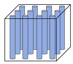
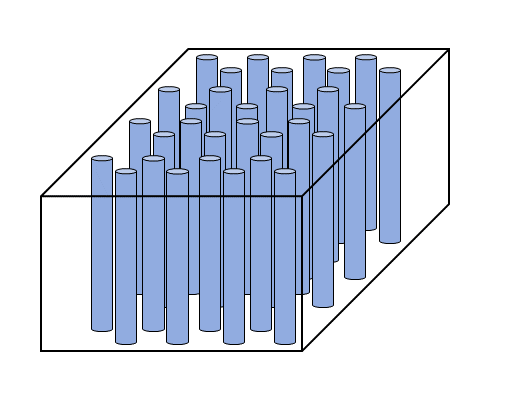
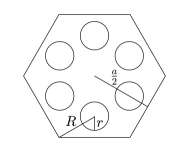
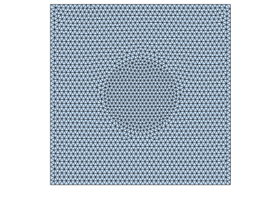
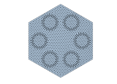
Figure 1: A schematic illustration of 2D PhCs. The materials have dielectric columns homogeneous along the z𝑧z direction and periodic along x𝑥x and y𝑦y directions.

In this work, we focus on 2D PhCs. In Figure 1, we show 2D PhCs with a periodic arrangement of dielectric columns within a dielectric material. In practice, both have finite extensions in the z𝑧z direction and finite periodicities in the x𝑥x-y𝑦y plane. Nevertheless, it is commonly assumed that the material extends infinitely in the plane perpendicular to the columns. Thus, in the setting of 2D PhCs in Figure 1, the relative permittivity ϵ(𝐱)italic-ϵ𝐱\epsilon(\mathbf{x}) is assumed to be independent of the z𝑧z direction. Then we can split the electromagnetic fields 𝐄=(E1,E2,E3)𝐄subscript𝐸1subscript𝐸2subscript𝐸3\mathbf{E}=(E_{1},E_{2},E_{3}) and 𝐇=(H1,H2,H3)𝐇subscript𝐻1subscript𝐻2subscript𝐻3\mathbf{H}=(H_{1},H_{2},H_{3}) in (2.2) and (2.3) into the transverse electric (TE) mode with H1=H2=E3=0subscript𝐻1subscript𝐻2subscript𝐸30H_{1}=H_{2}=E_{3}=0 and transverse magnetic (TM) mode with E1=E2=H3=0subscript𝐸1subscript𝐸2subscript𝐻30E_{1}=E_{2}=H_{3}=0. Each mode is a scalar eigenvalue problem,

(ϵ(𝐱)1H(𝐱))(ωc1)2H(𝐱)italic-ϵsuperscript𝐱1𝐻𝐱superscript𝜔superscript𝑐12𝐻𝐱\displaystyle-\nabla\cdot(\epsilon(\mathbf{x})^{-1}\nabla H(\mathbf{x}))-(\omega c^{-1})^{2}H(\mathbf{x}) =0,𝐱2,formulae-sequenceabsent0𝐱superscript2\displaystyle=0,\quad\mathbf{x}\in\mathbb{R}^{2}, (TE mode),(TE mode)\displaystyle\textbf{(TE mode)}, (2.4)
ΔE(𝐱)(ωc1)2ϵ(𝐱)E(𝐱)Δ𝐸𝐱superscript𝜔superscript𝑐12italic-ϵ𝐱𝐸𝐱\displaystyle-\Delta E(\mathbf{x})-(\omega c^{-1})^{2}\epsilon(\mathbf{x})E(\mathbf{x}) =0,𝐱2,formulae-sequenceabsent0𝐱superscript2\displaystyle=0,\quad\mathbf{x}\in\mathbb{R}^{2}, (TM mode).(TM mode)\displaystyle\textbf{(TM mode)}. (2.5)
Refer to caption
Refer to caption
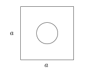
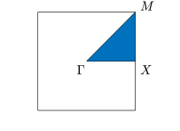
Figure 2: Square lattice: ΩΩ\Omega (left) and the corresponding Brillouin zone (right). The IBZ \mathcal{B}

is the shaded triangle with vertices Γ=(0,0)Γ00\Gamma=(0,0), X=1a(π,0)𝑋1𝑎𝜋0X=\frac{1}{a}(\pi,0) and M=1a(π,π)𝑀1𝑎𝜋𝜋M=\frac{1}{a}(\pi,\pi).

Refer to caption
Refer to caption
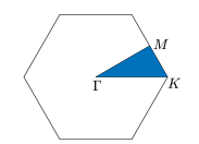
Figure 3: Hexagonal lattice: ΩΩ\Omega (left) and the corresponding Brillouin zone (right). The IBZ \mathcal{B}

is the shaded triangle with vertices Γ=(0,0)Γ00\Gamma=(0,0), K=1a(43π,0)𝐾1𝑎43𝜋0K=\frac{1}{a}(\frac{4}{3}\pi,0) and M=1a(π,33π)𝑀1𝑎𝜋33𝜋M=\frac{1}{a}(\pi,\frac{\sqrt{3}}{3}\pi).

2D PhCs possess a discrete translational symmetry in the x𝑥x-y𝑦y plane (cf. Figure 1) [16], i.e., the relative permittivity ϵ(𝐱)italic-ϵ𝐱\epsilon(\mathbf{x}) satisfies

ϵ(𝐱+c1𝐚1+c2𝐚2)=ϵ(𝐱),𝐱2 and c1,c2.formulae-sequenceitalic-ϵ𝐱subscript𝑐1subscript𝐚1subscript𝑐2subscript𝐚2italic-ϵ𝐱formulae-sequencefor-all𝐱superscript2 and subscript𝑐1subscript𝑐2\epsilon(\mathbf{x}+c_{1}\mathbf{a}_{1}+c_{2}\mathbf{a}_{2})=\epsilon(\mathbf{x}),\quad\forall\mathbf{x}\in\mathbb{R}^{2}\text{ and }c_{1},c_{2}\in\mathbb{Z}.

The primitive lattice vectors, denoted by 𝐚1subscript𝐚1\mathbf{a}_{1} and 𝐚2subscript𝐚2\mathbf{a}_{2}, are the shortest possible vectors that fulfill this condition and they span the fundamental periodicity domain ΩΩ\Omega, also known as unit cell, cf. Figures 2 and 3. In Figure 2, primitive lattice vectors of the square lattice are 𝐚i=aeisubscript𝐚𝑖𝑎subscript𝑒𝑖\mathbf{a}_{i}=a{e}_{i} for i=1,2𝑖12i=1,2, and in Figure 3, that of the hexagonal lattice 𝐚1=a4(e1+3e2)subscript𝐚1𝑎4subscript𝑒13subscript𝑒2\mathbf{a}_{1}=\frac{a}{4}({e}_{1}+\sqrt{3}{e}_{2}) and 𝐚2=a4(e13e2)subscript𝐚2𝑎4subscript𝑒13subscript𝑒2\mathbf{a}_{2}=\frac{a}{4}({e}_{1}-\sqrt{3}{e}_{2}). Here, (ei)i=1,2subscriptsubscript𝑒𝑖𝑖12(e_{i})_{i=1,2} is the canonical basis in 2superscript2\mathbb{R}^{2} and a+𝑎superscripta\in\mathbb{R}^{+} lattice constant. The reciprocal lattice vectors are defined by

𝐛i𝐚j=2πδij, for i,j=1,2,formulae-sequencesubscript𝐛𝑖subscript𝐚𝑗2𝜋subscript𝛿𝑖𝑗 for 𝑖𝑗12\mathbf{b}_{i}\cdot\mathbf{a}_{j}=2\pi\delta_{ij},\quad\text{ for }i,j=1,2, (2.6)

which generate the so-called reciprocal lattice. The elementary cell of the reciprocal lattice is the (first) Brillouin zone Fsubscript𝐹\mathcal{B}_{F}, i.e., the region closer to a certain lattice point than to any other lattice points in the reciprocal lattice.

Bloch’s theorem [20] states that in periodic crystals, wave functions take the form of a plane wave modulated by a periodic function. Thus they can be written as Ψ(𝐱)=ei𝐤𝐱u(𝐱)Ψ𝐱superscript𝑒𝑖𝐤𝐱𝑢𝐱\Psi(\mathbf{x})=e^{i\mathbf{k}\cdot\mathbf{x}}u(\mathbf{x}), where ΨΨ\Psi is the wave function, u(𝐱)𝑢𝐱u(\mathbf{x}) is periodic sharing the periodicity of the crystal lattice and 𝐤𝐤\mathbf{k} is the wave vector varying in the Brillouin zone Fsubscript𝐹\mathcal{B}_{F}. The periodic condition of u(𝐱)𝑢𝐱u(\mathbf{x}) implies that each wave function can be determined by its values within the unit cell ΩΩ\Omega. Thus, the solutions to (2.4) and (2.5) can be expressed as H(𝐱)=ei𝐤𝐱u1(𝐱)𝐻𝐱superscript𝑒𝑖𝐤𝐱subscript𝑢1𝐱H(\mathbf{x})=e^{i\mathbf{k}\cdot\mathbf{x}}u_{1}(\mathbf{x}) and E(𝐱)=ei𝐤𝐱u2(𝐱)𝐸𝐱superscript𝑒𝑖𝐤𝐱subscript𝑢2𝐱E(\mathbf{x})=e^{i\mathbf{k}\cdot\mathbf{x}}u_{2}(\mathbf{x}) for some periodic functions u1(𝐱)subscript𝑢1𝐱u_{1}(\mathbf{x}) and u2(𝐱)subscript𝑢2𝐱u_{2}(\mathbf{x}) in the unit cell ΩΩ\Omega, and the parameterized Helmholtz eigenvalue problems (2.4) and (2.5) reduce to

(+i𝐤)(ϵ(𝐱)1(+i𝐤)u1(𝐱))(ωc1)2u1(𝐱)𝑖𝐤italic-ϵsuperscript𝐱1𝑖𝐤subscript𝑢1𝐱superscript𝜔superscript𝑐12subscript𝑢1𝐱\displaystyle-(\nabla+i\mathbf{k})\cdot\left(\epsilon(\mathbf{x})^{-1}(\nabla+i\mathbf{k})u_{1}(\mathbf{x})\right)-\left(\omega c^{-1}\right)^{2}u_{1}(\mathbf{x}) =0,𝐱Ωformulae-sequenceabsent0𝐱Ω\displaystyle=0,\quad\mathbf{x}\in\Omega (TE mode),(TE mode)\displaystyle\textbf{(TE mode)}, (2.7a)
(+i𝐤)((+i𝐤)u2(𝐱))(ωc1)2ϵ(𝐱)u2(𝐱)𝑖𝐤𝑖𝐤subscript𝑢2𝐱superscript𝜔superscript𝑐12italic-ϵ𝐱subscript𝑢2𝐱\displaystyle-(\nabla+i\mathbf{k})\cdot\left((\nabla+i\mathbf{k})u_{2}(\mathbf{x})\right)-\left(\omega c^{-1}\right)^{2}\epsilon(\mathbf{x})u_{2}(\mathbf{x}) =0,𝐱Ωformulae-sequenceabsent0𝐱Ω\displaystyle=0,\quad\mathbf{x}\in\Omega (TM mode),(TM mode)\displaystyle\textbf{(TM mode)}, (2.7b)

where 𝐱Ω2𝐱Ωsuperscript2\mathbf{x}\in\Omega\subset\mathbb{R}^{2}, 𝐤𝐤\mathbf{k} varies in the Brillouin zone (BZ), and ui(𝐱)subscript𝑢𝑖𝐱u_{i}(\mathbf{x}) satisfies the periodic boundary conditions ui(𝐱)=ui(𝐱+𝐚𝐣)subscript𝑢𝑖𝐱subscript𝑢𝑖𝐱subscript𝐚𝐣u_{i}(\mathbf{x})=u_{i}(\mathbf{x}+\mathbf{a_{j}}) with 𝐚𝐣subscript𝐚𝐣\mathbf{a_{j}} being the primitive lattice vector for i,j=1,2formulae-sequence𝑖𝑗12i,j=1,2. If the materials in the unit cell have additional symmetry, e.g. mirror symmetry, we can further restrict 𝐤𝐤\mathbf{k} to the triangular irreducible Brillouin zone (IBZ), denoted by \mathcal{B}. The BZs and IBZs of the square lattice and hexagonal lattice are shown in Figures 2 and 3.

In sum, we can formulate both parameterized Helmholtz problems (2.7a) and (2.7b) by

(+i𝐤)α(𝐱)(+i𝐤)u(𝐱)λβ(𝐱)u(𝐱)=0,𝐱Ω,formulae-sequence𝑖𝐤𝛼𝐱𝑖𝐤𝑢𝐱𝜆𝛽𝐱𝑢𝐱0𝐱Ω-(\nabla+i\mathbf{k})\cdot\alpha(\mathbf{x})(\nabla+i\mathbf{k})u(\mathbf{x})-\lambda\beta(\mathbf{x})u(\mathbf{x})=0,\quad\mathbf{x}\in\Omega, (2.8)

with Ω2Ωsuperscript2\Omega\subset\mathbb{R}^{2}, 𝐤𝐤\mathbf{k}\in\mathcal{B}, and λ=(ωc1)2𝜆superscript𝜔superscript𝑐12\lambda=(\omega c^{-1})^{2}. In the TE mode, u𝑢u describes the magnetic field H𝐻H in z𝑧z-direction and the coefficients α(𝐱)𝛼𝐱\alpha(\mathbf{x}) and β(𝐱)𝛽𝐱\beta(\mathbf{x}) are α(𝐱):=ϵ(𝐱)1assign𝛼𝐱italic-ϵsuperscript𝐱1\alpha(\mathbf{x}):=\epsilon(\mathbf{x})^{-1} and β(𝐱):=1assign𝛽𝐱1\beta(\mathbf{x}):=1. Similarly, in the TM mode, u𝑢u describes the electric field E𝐸E in the z𝑧z-direction and the coefficients α(𝐱)𝛼𝐱\alpha(\mathbf{x}) and β(𝐱)𝛽𝐱\beta(\mathbf{x}) are α(𝐱):=1assign𝛼𝐱1\alpha(\mathbf{x}):=1 and β(𝐱):=ϵ(𝐱)assign𝛽𝐱italic-ϵ𝐱\beta(\mathbf{x}):=\epsilon(\mathbf{x}). The variational formulation of (2.8) reads: find a non-trivial eigenpair (λ,u)(,Hπ1(Ω))𝜆𝑢subscriptsuperscript𝐻1𝜋Ω(\lambda,u)\in(\mathbb{R},H^{1}_{\pi}(\Omega)) for 𝐤𝐤\mathbf{k}\in\mathcal{B} such that

{Ωα(+i𝐤)u(i𝐤)v¯λβuv¯dx=0,vHπ1(Ω)uLβ2(Ω)=1.\left\{\begin{aligned} \int_{\Omega}\alpha(\nabla+i\mathbf{k})u\cdot(\nabla-i\mathbf{k})\bar{v}-\lambda\beta u\bar{v}\mathrm{d}x&=0,\quad\forall v\in H^{1}_{\pi}(\Omega)\\ \|u\|_{L^{2}_{\beta}(\Omega)}&=1.\end{aligned}\right. (2.9)

Here, we define Lβ2(Ω)subscriptsuperscript𝐿2𝛽ΩL^{2}_{\beta}(\Omega) as the space of weighted square integrable functions equipped with the norm fLβ2(Ω):=(Ωβ(𝐱)|f(𝐱)|2d𝐱)12assignsubscriptnorm𝑓subscriptsuperscript𝐿2𝛽ΩsuperscriptsubscriptΩ𝛽𝐱superscript𝑓𝐱2differential-d𝐱12\|f\|_{L^{2}_{\beta}(\Omega)}:=(\int_{\Omega}\beta(\mathbf{x})|f(\mathbf{x})|^{2}\mathrm{d}\mathbf{x})^{\frac{1}{2}}. Let H1(Ω)Lβ2(Ω)superscript𝐻1Ωsubscriptsuperscript𝐿2𝛽ΩH^{1}(\Omega)\subset L^{2}_{\beta}(\Omega) be with square integrable gradient, equipped with the standard H1(Ω)superscript𝐻1ΩH^{1}(\Omega)-norm and Hπ1(Ω)H1(Ω)subscriptsuperscript𝐻1𝜋Ωsuperscript𝐻1ΩH^{1}_{\pi}(\Omega)\subset H^{1}(\Omega) is composed of functions with periodic boundary conditions. Using the sesquilinear forms

a(u,v)𝑎𝑢𝑣\displaystyle a(u,v) :=Ωα(+i𝐤)u(i𝐤)v¯dxandb(u,v):=Ωβuv¯dx,formulae-sequenceassignabsentsubscriptΩ𝛼𝑖𝐤𝑢𝑖𝐤¯𝑣differential-d𝑥andassign𝑏𝑢𝑣subscriptΩ𝛽𝑢¯𝑣differential-d𝑥\displaystyle:=\int_{\Omega}\alpha(\nabla+i\mathbf{k})u\cdot(\nabla-i\mathbf{k})\bar{v}\,\mathrm{d}x\quad\mbox{and}\quad b(u,v):=\int_{\Omega}\beta u\bar{v}\,\mathrm{d}x,

problem (2.9) is equivalent to finding a non-trivial eigenpair (λ,u)(,Hπ1(Ω))𝜆𝑢subscriptsuperscript𝐻1𝜋Ω(\lambda,u)\in(\mathbb{R},H^{1}_{\pi}(\Omega)) for 𝐤𝐤\mathbf{k}\in\mathcal{B} such that

{a(u,v)=λb(u,v), for all vHπ1(Ω)uLβ2(Ω)=1.\left\{\begin{aligned} a(u,v)&=\lambda b(u,v),\text{ for all }v\in H^{1}_{\pi}(\Omega)\\ \|u\|_{L^{2}_{\beta}(\Omega)}&=1.\end{aligned}\right. (2.10)

2.2 Regularity of band functions in the parameter domain

The regularity of band functions plays a crucial role in the convergence analysis. We have the following result taken from [34]. Here, Lip()𝐿𝑖𝑝Lip(\mathcal{B}) denotes the space of Lipschitz continuous functions in the IBZ \mathcal{B} and Å()̊𝐴\mathring{A}(\mathcal{B}) the space of piecewise analytic functions with singular point set of zero Lebesgue measure.

Theorem 2.1.

For 2D periodic PhCs, ωn(𝐤)Lip()Å()subscript𝜔𝑛𝐤𝐿𝑖𝑝̊𝐴\omega_{n}(\mathbf{k})\in Lip(\mathcal{B})\cap\mathring{A}(\mathcal{B}) for all n+𝑛subscriptn\in\mathbb{N}_{+}: each band function ωn(𝐤)subscript𝜔𝑛𝐤\omega_{n}(\mathbf{k}) is analytic in \𝐒\𝐒\mathcal{B}\backslash\mathbf{S}, where 𝐒𝐒\mathbf{S}\subset\mathcal{B} consists of the origin and points of degeneracy (i.e., the set of points at which certain band functions intersect, with zero Lebesgue measure).

Remark 2.1.

Note that the singularity at 𝐤=𝟎𝐤0\mathbf{k}=\mathbf{0} differs from that of others. The latter are known as branch points while the former arises from the composition gλ𝑔𝜆g\circ\lambda with g(x):=xassign𝑔𝑥𝑥g(x):=\sqrt{x}. The derivative of the first band function ω1(𝐤)=cλ1(𝐤)subscript𝜔1𝐤𝑐subscript𝜆1𝐤\omega_{1}(\mathbf{k})=c\cdot\sqrt{\lambda_{1}(\mathbf{k})}, which takes the value 00 at the origin, fail to be defined at 𝐤=𝟎𝐤0\mathbf{k}=\mathbf{0}. To remove the effect of this singularity, we approximate λj(𝐤)subscript𝜆𝑗𝐤\lambda_{j}(\mathbf{k}) for j=1,,L1𝑗1𝐿1j=1,\cdots,L-1 with 1<L1𝐿1<L\in\mathbb{N}, instead.

3 hp𝑝hp-adaptive sampling algorithm in the parameter domain

Due to the presence of singularities, the convergence of numerical methods based on global or fixed-order local polynomial interpolation on uniform meshes may be slow. To optimally deal with singular points of band functions in PhCs, we propose a novel efficient numerical algorithm using an hp𝑝hp-adaptive interpolation method. It is inspired by the celebrated hp𝑝hp FEM [2, 1], and employs nonuniformly distributed polynomial degrees over graded, nonuniform meshes to discretize the problem. We shall design an hp𝑝hp interpolation strategy based on an element-wise quantity in order to approximate the first L1𝐿1L-1 band functions for 1<L1𝐿1<L\in\mathbb{N}.

3.1 Adaptive mesh generation

We first recall the concept of a regular mesh without hanging nodes [27]. Let D2𝐷superscript2D\subset\mathbb{R}^{2} be a polygon with straight sides. A mesh 𝒯={Ti}i=1M𝒯superscriptsubscriptsubscript𝑇𝑖𝑖1𝑀\mathcal{T}=\{T_{i}\}_{i=1}^{M} is a partition of D𝐷D into open disjoint triangles Tisubscript𝑇𝑖T_{i} with D¯=i=1MTi¯¯𝐷superscriptsubscript𝑖1𝑀¯subscript𝑇𝑖\overline{D}=\cup_{i=1}^{M}\overline{T_{i}}. For each T𝒯𝑇𝒯T\in\mathcal{T}, we denote by hTsubscript𝑇h_{T} its diameter and ρTsubscript𝜌𝑇\rho_{T} the diameter of the largest inscribed ball.

Definition 3.1.

A mesh 𝒯={Ti}i=1M𝒯superscriptsubscriptsubscript𝑇𝑖𝑖1𝑀\mathcal{T}=\{T_{i}\}_{i=1}^{M} is said to be a regular mesh without hanging nodes if the following conditions hold. (i) For ij𝑖𝑗i\neq j, Ti¯Tj¯¯subscript𝑇𝑖¯subscript𝑇𝑗\overline{T_{i}}\cap\overline{T_{j}} is either empty or it consists of a vertex or an entire edge of Tisubscript𝑇𝑖T_{i} and (ii) There exists a constant C>0𝐶0C>0 such that hTCρTsubscript𝑇𝐶subscript𝜌𝑇h_{T}\leq C\rho_{T}.

We shall develop a strategy to generate a family of nested regular triangular meshes 𝒯nsubscript𝒯𝑛\mathcal{T}_{n}, n=1,2,𝑛12n=1,2,\cdots, based on an element-wise quantity (3.1) and a criterion for refinement (3.2). We need several notations for the mesh 𝒯nsubscript𝒯𝑛\mathcal{T}_{n}. The mesh size of 𝒯nsubscript𝒯𝑛\mathcal{T}_{n} is denoted by hn:=maxT𝒯nhTassignsubscript𝑛subscript𝑇subscript𝒯𝑛subscript𝑇h_{n}:=\max_{T\in\mathcal{T}_{n}}h_{T}. The collection of all faces and vertices over 𝒯nsubscript𝒯𝑛\mathcal{T}_{n} is denoted by nsubscript𝑛\mathcal{F}_{n} and 𝒱nsubscript𝒱𝑛\mathcal{V}_{n}, respectively. For any T𝒯n𝑇subscript𝒯𝑛T\in\mathcal{T}_{n}, T:=Tnassignsubscript𝑇𝑇subscript𝑛\mathcal{F}_{T}:=\partial T\cap\mathcal{F}_{n} denotes its faces, and FTjsuperscriptsubscript𝐹𝑇𝑗F_{T}^{j} for j=1,2,3𝑗123j=1,2,3 the j𝑗jth face, 𝒱T:=T𝒱nassignsubscript𝒱𝑇𝑇subscript𝒱𝑛\mathcal{V}_{T}:=\partial T\cap\mathcal{V}_{n} its vertices, and VTjsuperscriptsubscript𝑉𝑇𝑗V_{T}^{j} for j=1,2,3𝑗123j=1,2,3 the j𝑗jth vertex. For any Fn𝐹subscript𝑛F\in\mathcal{F}_{n}, 𝒯F:={T𝒯n:FT}assignsubscript𝒯𝐹conditional-set𝑇subscript𝒯𝑛𝐹subscript𝑇\mathcal{T}_{F}:=\cup\{T\in\mathcal{T}_{n}:F\in\mathcal{F}_{T}\} denotes the collection of elements having F𝐹F as an edge. Finally, Pm(T)subscript𝑃𝑚𝑇P_{m}(T) is the space of polynomial functions of degrees at most m+𝑚subscriptm\in\mathbb{N}_{+} on element T𝑇T, and Pm(F)subscript𝑃𝑚𝐹P_{m}(F) the space of polynomial functions of degrees at most m+𝑚subscriptm\in\mathbb{N}_{+} on each face Fn𝐹subscript𝑛F\in\mathcal{F}_{n}.

Since each band function is a piecewise analytic function of the wave vector, with singular points at branch points and the origin, the mesh design strategy should identify elements in which adjacent bands are in close proximity, and then refine them suitably to minimize the impact of singularities on the approximation. To this end, we employ an element-wise indicator that is based on the distance between two adjacent band functions

η(T):=min1qL1ωqωq+1,𝒱T for T𝒯n.assign𝜂𝑇subscript1𝑞𝐿1subscriptnormsubscript𝜔𝑞subscript𝜔𝑞1subscript𝒱𝑇 for 𝑇subscript𝒯𝑛\eta(T):=\min_{1\leq q\leq L-1}\left\|\omega_{q}-\omega_{q+1}\right\|_{\infty,\mathcal{V}_{T}}\text{ for }T\in\mathcal{T}_{n}. (3.1)

That is, it uses the adjacent values on the vertices of each triangle element to ascertain the regularity of the band functions within each element. Furthermore, we introduce an element-wise tolerance

tol1(T)=κhTmax1qLωq,T\𝐒,subscripttol1𝑇𝜅subscript𝑇subscript1𝑞𝐿subscriptnormsubscript𝜔𝑞\𝑇𝐒\operatorname{tol}_{1}(T)=\kappa h_{T}\max_{1\leq q\leq L}\|\nabla\omega_{q}\|_{\infty,T\backslash\mathbf{S}}, (3.2)

where 𝐒𝐒\mathbf{S} is the set of singular points and κ22𝜅22\kappa\geq 2\sqrt{2} is a constant. The band function ωq(𝐤)subscript𝜔𝑞𝐤\omega_{q}(\mathbf{k}) and the group velocity ωq(𝐤)subscript𝜔𝑞𝐤\nabla\omega_{q}(\mathbf{k}) used in η(T)𝜂𝑇\eta(T) and tol1(T)subscripttol1𝑇\operatorname{tol}_{1}(T) are computed using the conforming Galerkin FEM, cf. (2.10) and (3.9).

Give a mesh 𝒯nsubscript𝒯𝑛\mathcal{T}_{n}, the collection of marked elements is

n:={T𝒯n:η(T)tol1(T)}.assignsubscript𝑛conditional-set𝑇subscript𝒯𝑛𝜂𝑇subscripttol1𝑇\displaystyle\mathcal{M}_{n}:=\cup\left\{T\in\mathcal{T}_{n}:\eta(T)\leq\operatorname{tol}_{1}(T)\right\}. (3.3)

We employ the iterated newest vertex bisection (NVB) [11] to refine the elements in nsubscript𝑛\mathcal{M}_{n}. It involves repeatedly bisecting the longest edge of the marked element and inserting a new vertex at the midpoint until the desired level of refinement is achieved. Then the resulting mesh is sufficiently refined in areas where the singularities may impact the approximation accuracy.

Iterated NVB preserves the mesh regularity during refinement [32]. However, to achieve a set of regular meshes without any hanging nodes, it is often necessary to refine certain elements beyond the initial refinement. Thus, the number of elements to be refined, denoted as #𝒯n+1#𝒯n#subscript𝒯𝑛1#subscript𝒯𝑛\#\mathcal{T}_{n+1}-\#\mathcal{T}_{n}, is typically larger than the number of marked elements #n#subscript𝑛\#\mathcal{M}_{n}. Nonetheless, the cumulative number of elements added in this manner does not inflate the total number of marked elements [4, Theorem 2.4].

Theorem 3.1.

Let 𝒯1subscript𝒯1\mathcal{T}_{1} be a regular mesh in the sense of Definition 3.1. For n1𝑛1n\geq 1 let {𝒯n}n1subscriptsubscript𝒯𝑛𝑛1\{\mathcal{T}_{n}\}_{n\geq 1} be any sequence of the refinement of 𝒯1subscript𝒯1\mathcal{T}_{1}, where 𝒯n+1subscript𝒯𝑛1\mathcal{T}_{n+1} is a regular mesh generated from 𝒯nsubscript𝒯𝑛\mathcal{T}_{n} by the iterated NVB with a subset of the marked elements n𝒯nsubscript𝑛subscript𝒯𝑛\mathcal{M}_{n}\subset\mathcal{T}_{n}. Then there exists a constant C𝐶C solely depending on 𝒯1subscript𝒯1\mathcal{T}_{1} such that

#𝒯n#𝒯1Ci=1n1#i,n1.formulae-sequence#subscript𝒯𝑛#subscript𝒯1𝐶superscriptsubscript𝑖1𝑛1#subscript𝑖for-all𝑛1\#\mathcal{T}_{n}-\#\mathcal{T}_{1}\leq C\sum_{i=1}^{n-1}\#\mathcal{M}_{i},\quad\forall n\geq 1. (3.4)

We give the proposed mesh refinement procedure in Algorithm 1. The parameters tol2subscripttol2\operatorname{tol}_{2} and nmaxsubscript𝑛n_{\max} denote the smallest allowed element size and the maximum number of iterations, respectively.

Algorithm 1 Adaptive mesh refinement
initial mesh 𝒯1subscript𝒯1\mathcal{T}_{1}, tolerance tol2subscripttol2\operatorname{tol}_{2}, and maximum loop number nmaxsubscript𝑛n_{\max}
𝒯nsubscript𝒯𝑛\mathcal{T}_{n}
n1𝑛1n\leftarrow 1
while nnmax𝑛subscript𝑛n\leq n_{\max} do
     Set n=subscript𝑛\mathcal{M}_{n}=\emptyset
     for T𝒯n𝑇subscript𝒯𝑛T\in\mathcal{T}_{n} do
         if η(T)tol1(T)𝜂𝑇subscripttol1𝑇\eta(T)\leq\operatorname{tol}_{1}(T) and hTtol2subscript𝑇subscripttol2h_{T}\geq\operatorname{tol}_{2} then
              n=n{T}subscript𝑛subscript𝑛𝑇\mathcal{M}_{n}=\mathcal{M}_{n}\cup\{T\}
         end if
     end forRefine the collection of marked elements nsubscript𝑛\mathcal{M}_{n} by iterated NVB and adjust the mesh until there are no hanging nodes. nn+1𝑛𝑛1n\leftarrow n+1
end while

3.2 Reliability of Algorithm 1

For the mesh 𝒯nsubscript𝒯𝑛\mathcal{T}_{n} at the n𝑛nth iteration, let

𝒯nR:={T𝒯n:T𝐒=} and 𝒯nS:=𝒯n\𝒯nRassignsuperscriptsubscript𝒯𝑛𝑅conditional-set𝑇subscript𝒯𝑛𝑇𝐒 and superscriptsubscript𝒯𝑛𝑆assign\subscript𝒯𝑛superscriptsubscript𝒯𝑛𝑅\displaystyle\mathcal{T}_{n}^{R}:=\cup\left\{T\in\mathcal{T}_{n}:T\cap\mathbf{S}=\emptyset\right\}\text{ and }\mathcal{T}_{n}^{S}:=\mathcal{T}_{n}\backslash\mathcal{T}_{n}^{R}

be a partition of the mesh 𝒯nsubscript𝒯𝑛\mathcal{T}_{n} based on the singular point set 𝐒𝐒\mathbf{S}. The next result guarantees that Algorithm 1 refines all the elements in 𝒯nSsuperscriptsubscript𝒯𝑛𝑆\mathcal{T}_{n}^{S} at the next iteration.

Theorem 3.2 (𝒯nSnsuperscriptsubscript𝒯𝑛𝑆subscript𝑛\mathcal{T}_{n}^{S}\subset\mathcal{M}_{n}).

Algorithm 1 with the element-wise quantity (3.1) and the tolerance (3.2) guarantees that all elements containing branch points are marked for refinement.

Proof.

The proof relies on piecewise analyticity and Lipschitz continuity of band functions. Let 𝒯nsubscript𝒯𝑛\mathcal{T}_{n} be a regular mesh generated by Algorithm 1 for n=1,𝑛1n=1,\cdots. For any band function ω(𝐤)𝜔𝐤\omega(\mathbf{k}) and any element T𝒯nR𝑇superscriptsubscript𝒯𝑛𝑅T\in\mathcal{T}_{n}^{R}, by the mean value theorem, we obtain

max𝐤T,𝐤^𝒱T|ω(𝐤)ω(𝐤^)|2hTω,T.subscriptformulae-sequence𝐤𝑇^𝐤subscript𝒱𝑇𝜔𝐤𝜔^𝐤2subscript𝑇subscriptnorm𝜔𝑇\max_{\begin{subarray}{c}\mathbf{k}\in T,\widehat{\mathbf{k}}\in\mathcal{V}_{T}\end{subarray}}|\omega(\mathbf{k})-\omega(\widehat{\mathbf{k}})|\leq\sqrt{2}h_{T}\cdot\|\nabla\omega\|_{\infty,T}. (3.5)

If T𝒯nS𝑇superscriptsubscript𝒯𝑛𝑆T\in\mathcal{T}_{n}^{S}, then the first derivative of band functions may be discontinuous on singular points. The singular points on the line segment connecting 𝐤𝐤\mathbf{k} and 𝐤^^𝐤\widehat{\mathbf{k}} divide the segment into several small intervals. By applying the mean value theorem on each subinterval, we obtain

max𝐤T,𝐤^𝒱T|ω(𝐤)ω(𝐤^)|2hTω,T\𝐒.subscriptformulae-sequence𝐤𝑇^𝐤subscript𝒱𝑇𝜔𝐤𝜔^𝐤2subscript𝑇subscriptnorm𝜔\𝑇𝐒\max_{\begin{subarray}{c}\mathbf{k}\in T,\widehat{\mathbf{k}}\in\mathcal{V}_{T}\end{subarray}}|\omega(\mathbf{k})-\omega(\widehat{\mathbf{k}})|\leq\sqrt{2}h_{T}\cdot\|\nabla\omega\|_{\infty,T\backslash\mathbf{S}}. (3.6)

Note that Tn𝑇subscript𝑛T\notin\mathcal{M}_{n} implies any two adjacent band functions ωp(𝐤)subscript𝜔𝑝𝐤\omega_{p}(\mathbf{k}) and ωp+1(𝐤)subscript𝜔𝑝1𝐤\omega_{p+1}(\mathbf{k}) for 1p<L11𝑝𝐿11\leq p<L-1 satisfy

min𝐤^𝒱T|ωp(𝐤^)ωp+1(𝐤^)|>tol1(T)=κhTmax1qLωq,T\𝐒.subscript^𝐤subscript𝒱𝑇subscript𝜔𝑝^𝐤subscript𝜔𝑝1^𝐤subscripttol1𝑇𝜅subscript𝑇subscript1𝑞𝐿subscriptnormsubscript𝜔𝑞\𝑇𝐒\displaystyle\min_{\widehat{\mathbf{k}}\in\mathcal{V}_{T}}|\omega_{p}(\widehat{\mathbf{k}})-\omega_{p+1}(\widehat{\mathbf{k}})|>\operatorname{tol}_{1}(T)=\kappa h_{T}\cdot\max_{1\leq q\leq L}\|\nabla\omega_{q}\|_{\infty,T\backslash\mathbf{S}}.

By the triangle inequality, this further implies for any 𝐤^𝒱T^𝐤subscript𝒱𝑇\widehat{\mathbf{k}}\in\mathcal{V}_{T} and 𝐤T𝐤𝑇\mathbf{k}\in T,

tol1(T)subscripttol1𝑇\displaystyle\operatorname{tol}_{1}(T) <|ωp(𝐤^)ωp+1(𝐤^)|absentsubscript𝜔𝑝^𝐤subscript𝜔𝑝1^𝐤\displaystyle<|\omega_{p}(\widehat{\mathbf{k}})-\omega_{p+1}(\widehat{\mathbf{k}})|
|ωp(𝐤^)ωp(𝐤)|+|ωp(𝐤)ωp+1(𝐤)|+|ωp+1(𝐤)ωp+1(𝐤^)|.absentsubscript𝜔𝑝^𝐤subscript𝜔𝑝𝐤subscript𝜔𝑝𝐤subscript𝜔𝑝1𝐤subscript𝜔𝑝1𝐤subscript𝜔𝑝1^𝐤\displaystyle\leq|\omega_{p}(\widehat{\mathbf{k}})-\omega_{p}(\mathbf{k})|+|\omega_{p}(\mathbf{k})-\omega_{p+1}(\mathbf{k})|+|\omega_{p+1}(\mathbf{k})-\omega_{p+1}(\widehat{\mathbf{k}})|.

This, together with (3.5) and (3.6), leads to

min𝐤T|ωp(𝐤)ωp+1(𝐤)|>(κ22)hTmax1qLωq,T\𝐒0.subscript𝐤𝑇subscript𝜔𝑝𝐤subscript𝜔𝑝1𝐤𝜅22subscript𝑇subscript1𝑞𝐿subscriptnormsubscript𝜔𝑞\𝑇𝐒0\displaystyle\min_{\mathbf{k}\in T}|\omega_{p}(\mathbf{k})-\omega_{p+1}(\mathbf{k})|>(\kappa-2\sqrt{2})h_{T}\cdot\max_{1\leq q\leq L}\|\nabla\omega_{q}\|_{\infty,T\backslash\mathbf{S}}\geq 0. (3.7)

That is, there is no branch points in T𝑇T and T𝒯nS𝑇superscriptsubscript𝒯𝑛𝑆T\notin\mathcal{T}_{n}^{S}. Hence, we have proved that T𝒯nS𝑇superscriptsubscript𝒯𝑛𝑆T\notin\mathcal{T}_{n}^{S} if Tn𝑇subscript𝑛T\notin\mathcal{M}_{n}, or equivalently 𝒯nSnsuperscriptsubscript𝒯𝑛𝑆subscript𝑛\mathcal{T}_{n}^{S}\subset\mathcal{M}_{n}. ∎

Computing the element-wise tolerance tol1(T)subscripttol1𝑇\operatorname{tol}_{1}(T) (3.2) is impractical since it involves estimating ω(𝐤)subscriptnorm𝜔𝐤\|\nabla\omega(\mathbf{k})\|_{\infty} for all 𝐤T\𝐒𝐤\𝑇𝐒\mathbf{k}\in T\backslash\mathbf{S}. However, numerical experiments have shown that the slope of the first several band functions (a.k.a. group velocity) does not exhibit high oscillations. Hermann et al [13] showed that in the first three bands, higher bands have low values of the group velocity and all of them are curves without significant fluctuations. Therefore, as a substitute for tol1(T)subscripttol1𝑇\operatorname{tol}_{1}(T), we use a feasible tolerance

tol^1(T):=κhTmax1qLωq,𝒱T\𝐒.assignsubscript^tol1𝑇𝜅subscript𝑇subscript1𝑞𝐿subscriptnormsubscript𝜔𝑞\subscript𝒱𝑇𝐒\displaystyle\widehat{\operatorname{tol}}_{1}(T):=\kappa h_{T}\max_{1\leq q\leq L}\|\nabla\omega_{q}\|_{\infty,\mathcal{V}_{T}\backslash\mathbf{S}}. (3.8)

Computing tol^1(T)subscript^tol1𝑇\widehat{\operatorname{tol}}_{1}(T) only requires the band function and its partial derivative over the vertices. Moreover, the group velocity can be derived directly from the following expression [34]

ωki=2kimα(u,u)+mαi(u,u)2ω,𝜔subscript𝑘𝑖2subscript𝑘𝑖subscript𝑚𝛼𝑢𝑢subscript𝑚𝛼𝑖𝑢𝑢2𝜔\frac{\partial\omega}{\partial k_{i}}=\frac{2k_{i}m_{\alpha}(u,u)+m_{\alpha i}(u,u)}{2\omega}, (3.9)

where the bilinear forms mαi(,)subscript𝑚𝛼𝑖m_{\alpha i}(\cdot,\cdot) and mα(,)subscript𝑚𝛼m_{\alpha}(\cdot,\cdot) are defined as

mαi(u,v)=Ωiα(uv¯xiv¯uxi)d𝐱,i=1,2andmα(u,v)=Ωαuv¯d𝐱.formulae-sequencesubscript𝑚𝛼𝑖𝑢𝑣subscriptΩ𝑖𝛼𝑢¯𝑣subscript𝑥𝑖¯𝑣𝑢subscript𝑥𝑖differential-d𝐱formulae-sequence𝑖12andsubscript𝑚𝛼𝑢𝑣subscriptΩ𝛼𝑢¯𝑣differential-d𝐱\displaystyle m_{\alpha i}(u,v)=\int_{\Omega}i\alpha\left(u\frac{\partial\bar{v}}{\partial x_{i}}-\bar{v}\frac{\partial u}{\partial x_{i}}\right)\,\mathrm{d}\mathbf{x},\quad i=1,2\quad\mbox{and}\quad m_{\alpha}(u,v)=\int_{\Omega}\alpha u\bar{v}\,\mathrm{d}\mathbf{x}.

3.3 Conforming finite element space

Let {𝒯n}n=1superscriptsubscriptsubscript𝒯𝑛𝑛1\{\mathcal{T}_{n}\}_{n=1}^{\infty} be a sequence of nested regular triangular meshes generated by Algorithm 1. We shall construct an element-wise polynomial space for the mesh 𝒯nsubscript𝒯𝑛\mathcal{T}_{n}. We first define the layer of an element T𝒯n𝑇subscript𝒯𝑛T\in\mathcal{T}_{n} given by Algorithm 1.

Definition 3.2.

The layer Tsubscript𝑇\ell_{T} of an element T𝒯n𝑇subscript𝒯𝑛T\in\mathcal{T}_{n} is T:=nrassignsubscript𝑇𝑛𝑟\ell_{T}:=n-r, where 0rn10𝑟𝑛10\leq r\leq n-1 is the number of refinements that have been performed on this element in Algorithm 1.

Note that the layer Tsubscript𝑇\ell_{T} of an element T𝒯n𝑇subscript𝒯𝑛T\in\mathcal{T}_{n} implies the local regularity of the eigenfunction λj(𝐤)subscript𝜆𝑗𝐤\lambda_{j}(\mathbf{k}) for j=1,,L1𝑗1𝐿1j=1,\cdots,L-1. Since the singular points fall into the marked element nsubscript𝑛\mathcal{M}_{n}, we employ polynomials of lower degrees for the local interpolation in nsubscript𝑛\mathcal{M}_{n}. Note also that the first band function vanishes at the origin, and is non-negative, sharing the symmetry of the lattice. This leads to the expression of (ω1(𝐤))2superscriptsubscript𝜔1𝐤2\left(\omega_{1}(\mathbf{k})\right)^{2} similar to an elliptic cone. More precisely, since (ω1(𝐤))2superscriptsubscript𝜔1𝐤2\left(\omega_{1}(\mathbf{k})\right)^{2} is analytic at 𝐤=𝟎𝐤0\mathbf{k}=\mathbf{0} if ω1(𝟎)ω2(𝟎)subscript𝜔10subscript𝜔20\omega_{1}(\mathbf{0})\neq\omega_{2}(\mathbf{0}), its Taylor expansion at the origin is

(ω1(𝐤))2=(ω1(k1,k2))2=i=1j=0iaij(k1)2j(k2)2i2j,superscriptsubscript𝜔1𝐤2superscriptsubscript𝜔1subscript𝑘1subscript𝑘22superscriptsubscript𝑖1superscriptsubscript𝑗0𝑖subscript𝑎𝑖𝑗superscriptsubscript𝑘12𝑗superscriptsubscript𝑘22𝑖2𝑗\left(\omega_{1}(\mathbf{k})\right)^{2}=\left(\omega_{1}(k_{1},k_{2})\right)^{2}=\sum_{i=1}^{\infty}\sum_{j=0}^{i}a_{ij}\left(k_{1}\right)^{2j}\left(k_{2}\right)^{2i-2j},

with some aijsubscript𝑎𝑖𝑗a_{ij}\in\mathbb{R} for i𝑖i\in\mathbb{N} and j=0,,i𝑗0𝑖j=0,\cdots,i. Hence λ1(𝐤)=(ω1(𝐤)c1)2subscript𝜆1𝐤superscriptsubscript𝜔1𝐤superscript𝑐12\lambda_{1}(\mathbf{k})=(\omega_{1}(\mathbf{k})c^{-1})^{2} is quadratic near the origin, and we use polynomials of minimal degree 222 to interpolate eigenvalues over the marked elements nsubscript𝑛\mathcal{M}_{n}. These observations motivate the following definition of the element-wise space of polynomials. The notation \left\lceil\cdot\right\rceil denotes the ceiling function.

Definition 3.3.

For any element T𝒯n𝑇subscript𝒯𝑛T\in\mathcal{T}_{n}, we take PnT(T)subscript𝑃subscript𝑛𝑇𝑇P_{n_{T}}(T) as the local interpolation space, with nT:=max{2,μT}assignsubscript𝑛𝑇2𝜇subscript𝑇n_{T}:=\max\left\{2,\lceil\mu{\ell}_{T}\rceil\right\} if Tn𝑇subscript𝑛T\notin\mathcal{M}_{n}, and nT:=2assignsubscript𝑛𝑇2n_{T}:=2 otherwise, where the parameter μ>0𝜇0\mu>0 is determined in (5.9) in Section 5 and nsubscript𝑛\mathcal{M}_{n} is the collection of marked elements (3.3).

In this way, each element T𝑇T is assigned a total degree nTsubscript𝑛𝑇n_{T}. However, neighboring elements may have different degrees on the common face. Suitable constraints are required to ensure the inter-element continuity, for which it is essential to associate with each face in the mesh a face degree.

Definition 3.4 (Facewise space of polynomial functions).

Let PmF(F)subscript𝑃subscript𝑚𝐹𝐹P_{m_{F}}(F) be the local interpolation space over F𝐹F for Fn𝐹subscript𝑛F\in\mathcal{F}_{n} with mF:=minT𝒯F{nT}assignsubscript𝑚𝐹subscript𝑇subscript𝒯𝐹subscript𝑛𝑇m_{F}:=\min_{T\in\mathcal{T}_{F}}\{n_{T}\}. This implies maxFT{mF}nT, for all T𝒯nformulae-sequencesubscript𝐹subscript𝑇subscript𝑚𝐹subscript𝑛𝑇 for all 𝑇subscript𝒯𝑛\max_{F\in\mathcal{F}_{T}}\{m_{F}\}\leq n_{T},\text{ for all }T\in\mathcal{T}_{n}.

Finally, on a given mesh 𝒯nsubscript𝒯𝑛\mathcal{T}_{n} with element-wise and facewise degrees {nT}T𝒯nsubscriptsubscript𝑛𝑇𝑇subscript𝒯𝑛\{n_{T}\}_{T\in\mathcal{T}_{n}} and {mF}Fnsubscriptsubscript𝑚𝐹𝐹subscript𝑛\{m_{F}\}_{F\in\mathcal{F}_{n}}, we define the conforming FEM space

Vn:={vC():v|TPnT(T) and v|FPmF(F),T𝒯n and Fn},assignsubscript𝑉𝑛conditional-set𝑣𝐶formulae-sequenceevaluated-at𝑣𝑇evaluated-atsubscript𝑃subscript𝑛𝑇𝑇 and 𝑣𝐹subscript𝑃subscript𝑚𝐹𝐹for-all𝑇subscript𝒯𝑛 and 𝐹subscript𝑛\displaystyle V_{n}:=\left\{v\in C(\mathcal{B}):v|_{T}\in P_{n_{T}}(T)\text{ and }v|_{F}\in P_{m_{F}}(F),\,\forall T\in\mathcal{T}_{n}\text{ and }F\in\mathcal{F}_{n}\right\}, (3.10)

which is a space of continuous piecewise polynomial functions on \mathcal{B}. Let N𝑁N be its dimension. We aim at approximating the eigenvalues λ𝜆\lambda, for j=1,,L1𝑗1𝐿1j=1,\cdots,L-1, over Vnsubscript𝑉𝑛V_{n} by element-wise Lagrange interpolation.

4 Element-wise interpolation over the adaptive mesh

We develop Lagrange interpolation over each element T𝒯n𝑇subscript𝒯𝑛T\in\mathcal{T}_{n}. For each element, we first map its closure T¯¯𝑇\overline{T} into the reference equilateral triangle T^={𝐳:=(x,y):0y(1+x)3,1x0 or 0y(1x)3,0x1}^𝑇conditional-setassign𝐳𝑥𝑦formulae-sequence0𝑦1𝑥31𝑥0 or 0𝑦1𝑥30𝑥1\hat{T}=\{\mathbf{z}:=(x,y):0\leq y\leq(1+x)\sqrt{3},-1\leq x\leq 0\text{ or }0\leq y\leq(1-x)\sqrt{3},0\leq x\leq 1\} and then derive Lagrange interpolation on T^^𝑇\hat{T}. The vertices of T^^𝑇\hat{T} are 𝐳^1=(1,0)subscript^𝐳110\mathbf{\hat{z}}_{1}=(-1,0), 𝐳^2=(1,0)subscript^𝐳210\mathbf{\hat{z}}_{2}=(1,0) and 𝐳^3=(0,3)subscript^𝐳303\mathbf{\hat{z}}_{3}=(0,\sqrt{3}), with the face opposite to 𝐳^isubscript^𝐳𝑖\mathbf{\hat{z}}_{i} denoted by F^isuperscript^𝐹𝑖\hat{F}^{i}. For any {m,m1,m2,m3}+4𝑚subscript𝑚1subscript𝑚2subscript𝑚3superscriptsubscript4\{m,m_{1},m_{2},m_{3}\}\in\mathbb{N}_{+}^{4} with mmi𝑚subscript𝑚𝑖m\geq m_{i} for i=1,2,3𝑖123i=1,2,3, (3.10) implies that the local space of polynomial functions over T^^𝑇\hat{T} is

P^:={vPm(T^):v|F^iPmi(F^i)}.assign^𝑃conditional-set𝑣subscript𝑃𝑚^𝑇evaluated-at𝑣superscript^𝐹𝑖subscript𝑃subscript𝑚𝑖superscript^𝐹𝑖\displaystyle\hat{P}:=\{v\in P_{m}(\hat{T}):v|_{\hat{F}^{i}}\in P_{m_{i}}(\hat{F}^{i})\}. (4.1)

Note that P^Pm(T^)^𝑃subscript𝑃𝑚^𝑇\hat{P}\subset P_{m}(\hat{T}) and P^Pm(T^)^𝑃subscript𝑃𝑚^𝑇\hat{P}\subsetneq P_{m}(\hat{T}) if mi<msubscript𝑚𝑖𝑚m_{i}<m for some i=1,2,3𝑖123i=1,2,3. Note also that the dimension of Pm(T^)subscript𝑃𝑚^𝑇P_{m}(\hat{T}) is dim(Pm(T^))=(m+1)(m+2)/2dimensionsubscript𝑃𝑚^𝑇𝑚1𝑚22\dim(P_{m}(\hat{T}))=(m+1)(m+2)/2, and the dimension of P^^𝑃\hat{P} is dim(P^)=dim(Pm(T^))i=13(mmi)=3+((m11)+(m21)+(m31))+(m2)(m1)/2.dimension^𝑃dimensionsubscript𝑃𝑚^𝑇superscriptsubscript𝑖13𝑚subscript𝑚𝑖3subscript𝑚11subscript𝑚21subscript𝑚31𝑚2𝑚12\dim(\hat{P})=\dim(P_{m}(\hat{T}))-\sum_{i=1}^{3}(m-m_{i})=3+\big{(}(m_{1}-1)+(m_{2}-1)+(m_{3}-1)\big{)}+(m-2)(m-1)/2.

4.1 Basis functions in the local polynomial space P^^𝑃\hat{P}

We construct a set of basis functions for the local polynomial space P^^𝑃\hat{P}, following [27]. We divide the basis functions into external and internal shape functions according to whether they vanish over the boundary T^^𝑇\partial\hat{T}, and then divide the external shape functions further into nodal and side ones. The definition of nodal, side and internal shape functions is standard in the community of p𝑝p-version and hp𝑝hp-adaptive FEMs, and it enables defining conforming FEM spaces with nonuniform degrees of polynomials over the mesh. We focus on developing an element-wise interpolation, and these shape functions play a role when formulating a special local polynomial space P^^𝑃\hat{P}, which facilitates the definition of the element-wise interpolation in Section 4.2.

First, there are three nodal shape functions on T^^𝑇\hat{T}:

N11=(1xy/3)/2,N21=(1+xy/3)/2andN31=y/3.formulae-sequencesubscriptsuperscript𝑁111𝑥𝑦32formulae-sequencesubscriptsuperscript𝑁121𝑥𝑦32andsubscriptsuperscript𝑁13𝑦3N^{1}_{1}=(1-x-y/\sqrt{3})/2,\quad N^{1}_{2}=(1+x-y/\sqrt{3})/2\quad\mbox{and}\quad N^{1}_{3}=y/\sqrt{3}. (4.2)

Note that for i=1,2,3𝑖123i=1,2,3, we have Ni1(𝐳^i)=1subscriptsuperscript𝑁1𝑖subscript^𝐳𝑖1N^{1}_{i}(\mathbf{\hat{z}}_{i})=1 and Ni1(𝐳)=0subscriptsuperscript𝑁1𝑖𝐳0N^{1}_{i}(\mathbf{z})=0 for 𝐳F^i𝐳superscript^𝐹𝑖\mathbf{z}\in\hat{F}^{i}. Second, there are mi1subscript𝑚𝑖1m_{i}-1 side shape functions over F^isuperscript^𝐹𝑖\hat{F}^{i}, i=1,2,3𝑖123i=1,2,3, defined by

Nimi,jsubscriptsuperscript𝑁subscript𝑚𝑖𝑗𝑖\displaystyle N^{m_{i},j}_{i} =Ni+11Ni+21Φj2(Ni+21Ni+11),absentsubscriptsuperscript𝑁1𝑖1subscriptsuperscript𝑁1𝑖2subscriptΦ𝑗2subscriptsuperscript𝑁1𝑖2subscriptsuperscript𝑁1𝑖1\displaystyle=N^{1}_{i+1}N^{1}_{i+2}\Phi_{j-2}(N^{1}_{i+2}-N^{1}_{i+1}), (4.3)

with Φj2(x)subscriptΦ𝑗2𝑥\Phi_{j-2}(x) being a polynomial of degree j2𝑗2j-2 for j=2,,mi𝑗2subscript𝑚𝑖j=2,\cdots,m_{i}, with the convention Nj+31=Nj1superscriptsubscript𝑁𝑗31superscriptsubscript𝑁𝑗1N_{j+3}^{1}=N_{j}^{1} and 𝐳^j+3=𝐳^jsubscript^𝐳𝑗3subscript^𝐳𝑗\mathbf{\hat{z}}_{j+3}=\mathbf{\hat{z}}_{j} for j=1,2,3𝑗123j=1,2,3. Note that supp(Nimi,j)suppsubscriptsuperscript𝑁subscript𝑚𝑖𝑗𝑖\text{supp}(N^{m_{i},j}_{i}) is the interior of F^isuperscript^𝐹𝑖\hat{F}^{i} and T^^𝑇\hat{T}. Then the set of external shape functions is given by

m(m1,m2,m3)(T^):={Nj1,Njmj,i: 1j3 and 2imj}.assignsuperscriptsubscript𝑚subscript𝑚1subscript𝑚2subscript𝑚3^𝑇conditional-setsubscriptsuperscript𝑁1𝑗subscriptsuperscript𝑁subscript𝑚𝑗𝑖𝑗1𝑗3 and 2𝑖subscript𝑚𝑗\mathcal{E}_{m}^{(m_{1},m_{2},m_{3})}(\hat{T}):=\left\{N^{1}_{j},N^{m_{j},i}_{j}:\;1\leq j\leq 3\text{ and }2\leq i\leq m_{j}\right\}.

By construction, the number of external basis functions is 3+((m11)+(m21)+(m31))3subscript𝑚11subscript𝑚21subscript𝑚313+\big{(}(m_{1}-1)+(m_{2}-1)+(m_{3}-1)\big{)}.

Next, we construct a set of internal basis functions that vanish over T^^𝑇\partial\hat{T}. Let bT^:=N11N21N31assignsubscript𝑏^𝑇subscriptsuperscript𝑁11subscriptsuperscript𝑁12subscriptsuperscript𝑁13b_{\hat{T}}:=N^{1}_{1}N^{1}_{2}N^{1}_{3} be the basic bubble function on the reference element T^^𝑇\hat{T} that vanishes over the edge T^^𝑇\partial\hat{T}. Then the internal polynomial space m(T^)subscript𝑚^𝑇\mathcal{I}_{m}(\hat{T}) is defined by

m(T^):=span{bT^v|vPm3(T^)} for m3.assignsubscript𝑚^𝑇spanconditional-setsubscript𝑏^𝑇𝑣𝑣subscript𝑃𝑚3^𝑇 for 𝑚3\mathcal{I}_{m}(\hat{T}):=\text{span}\{b_{\hat{T}}v|v\in P_{m-3}(\hat{T})\}\text{ for }m\geq 3. (4.4)

The dimension of m(T^)subscript𝑚^𝑇\mathcal{I}_{m}(\hat{T}) is m^:=(m1)(m2)/2assign^𝑚𝑚1𝑚22\hat{m}:={(m-1)(m-2)}/{2}. Let one set of basis functions be denoted as

{N̊i:i=1,,m^}.conditional-setsubscript̊𝑁𝑖𝑖1^𝑚\{\mathring{N}_{i}:i=1,\cdots,\hat{m}\}. (4.5)

4.2 Local interpolation based on Lagrange polynomials

Now following [24], we construct a suitable interpolation operator Π:C(T^)P^:Π𝐶^𝑇^𝑃\Pi:C(\hat{T})\to\hat{P}, such that

{Πf|F^iPmi(F^i) for i=1,2,3,ΠfP^,fC(T^).\left\{\begin{aligned} \Pi f\big{|}_{\hat{F}^{i}}&\in P_{m_{i}}(\hat{F}^{i})\text{ for }i=1,2,3,\\ \Pi f&\in\hat{P},\end{aligned}\right.\quad\forall f\in C(\hat{T}).

It consists of the external interpolation E𝐸E and internal interpolation I𝐼I.

The external interpolation E𝐸E is an interpolation operator over Fekete points along each face. Since the boundary points of Fekete points are the one-dimensional Gauss-Lobatto points [10], we get the Gauss-Lobatto interpolation along each face F^isuperscript^𝐹𝑖\hat{F}^{i} for i=1,2,3𝑖123i=1,2,3. Next, we extend the polynomial Ef𝐸𝑓Ef to the domain ΩΩ\Omega, and denote the extension by 𝐄(Ef)𝐄𝐸𝑓\mathbf{E}(Ef). With the shape functions in Section 4.1, we can combine two procedures to obtain 𝐄(Ef)𝐄𝐸𝑓\mathbf{E}(Ef). Specifically, we use the nodal and side shape functions to perform external interpolation along each face on Fekete points. For example, for F^isuperscript^𝐹𝑖\hat{F}^{i} with i=1,2,3𝑖123i=1,2,3, the nodal shape functions are Ni+11superscriptsubscript𝑁𝑖11N_{i+1}^{1} and Ni+21superscriptsubscript𝑁𝑖21N_{i+2}^{1}, and we combine them with the (mi1)subscript𝑚𝑖1(m_{i}-1) side shape functions to obtain the interpolation on this face F^isuperscript^𝐹𝑖\hat{F}^{i}:

Ef|F^i=(j=2mici,jNimi,j+f(𝐳^i+1)Ni+11+f(𝐳^i+2)Ni+21)|F^i,evaluated-at𝐸𝑓superscript^𝐹𝑖evaluated-atsuperscriptsubscript𝑗2subscript𝑚𝑖subscript𝑐𝑖𝑗superscriptsubscript𝑁𝑖subscript𝑚𝑖𝑗𝑓subscript^𝐳𝑖1superscriptsubscript𝑁𝑖11𝑓subscript^𝐳𝑖2superscriptsubscript𝑁𝑖21superscript^𝐹𝑖Ef|_{\hat{F}^{i}}=\left(\sum_{j=2}^{m_{i}}c_{i,j}N_{i}^{m_{i},j}+f(\mathbf{\hat{z}}_{i+1})N_{i+1}^{1}+f(\mathbf{\hat{z}}_{i+2})N_{i+2}^{1}\right)\Bigg{|}_{\hat{F}^{i}}, (4.6)

where the coefficients {ci,j}j=2misuperscriptsubscriptsubscript𝑐𝑖𝑗𝑗2subscript𝑚𝑖\{c_{i,j}\}_{j=2}^{m_{i}} are to be determined such that Ef|F^ievaluated-at𝐸𝑓superscript^𝐹𝑖Ef|_{\hat{F}^{i}} interpolates the misubscript𝑚𝑖m_{i}th order Fekete points on the face F^isuperscript^𝐹𝑖\hat{F}^{i}.

The extension 𝐄(Ef)𝐄𝐸𝑓\mathbf{E}(Ef) of Ef𝐸𝑓Ef is then given by

𝐄(Ef)=i=13j=2mici,jNimi,j+i=13f(𝐳^i)Ni1.𝐄𝐸𝑓superscriptsubscript𝑖13superscriptsubscript𝑗2subscript𝑚𝑖subscript𝑐𝑖𝑗superscriptsubscript𝑁𝑖subscript𝑚𝑖𝑗superscriptsubscript𝑖13𝑓subscript^𝐳𝑖superscriptsubscript𝑁𝑖1\mathbf{E}(Ef)=\sum_{i=1}^{3}\sum_{j=2}^{m_{i}}c_{i,j}N_{i}^{m_{i},j}+\sum_{i=1}^{3}f(\mathbf{\hat{z}}_{i})N_{i}^{1}. (4.7)

One can easily verify that 𝐄(Ef)|F^i=Ef|F^ievaluated-at𝐄𝐸𝑓superscript^𝐹𝑖evaluated-at𝐸𝑓superscript^𝐹𝑖\mathbf{E}(Ef)\big{|}_{\hat{F}^{i}}=Ef\big{|}_{\hat{F}^{i}} for i=1,2,3𝑖123i=1,2,3.

Third, we define the internal interpolation operator I:C(T^)m(T^):𝐼𝐶^𝑇subscript𝑚^𝑇I:C(\hat{T})\to\mathcal{I}_{m}(\hat{T}) that interpolates the Fekete points {𝐳j}j=1m^superscriptsubscriptsuperscriptsubscript𝐳𝑗𝑗1^𝑚\{\mathbf{z}_{j}^{*}\}_{j=1}^{\hat{m}}, using the set of internal basis functions {N̊i:i=1,,m^}conditional-setsubscript̊𝑁𝑖𝑖1^𝑚\{\mathring{N}_{i}:i=1,\cdots,\hat{m}\} (4.5):

{𝐳j}j=1m^:=argmax{𝐳1,𝐳2,,𝐳m^}T^det(V(𝐳1,𝐳2,,𝐳m^)).assignsuperscriptsubscriptsuperscriptsubscript𝐳𝑗𝑗1^𝑚subscriptsubscript𝐳1subscript𝐳2subscript𝐳^𝑚^𝑇𝑉subscript𝐳1subscript𝐳2subscript𝐳^𝑚\displaystyle\{\mathbf{z}_{j}^{*}\}_{j=1}^{\hat{m}}:=\arg\max_{\{\mathbf{z}_{1},\mathbf{z}_{2},\cdots,\mathbf{z}_{\hat{m}}\}\subset\hat{T}}\det(V(\mathbf{z}_{1},\mathbf{z}_{2},\cdots,\mathbf{z}_{\hat{m}})). (4.8)

Here, V(𝐳1,𝐳2,,𝐳m^)m^×m^𝑉subscript𝐳1subscript𝐳2subscript𝐳^𝑚superscript^𝑚^𝑚V(\mathbf{z}_{1},\mathbf{z}_{2},\cdots,\mathbf{z}_{\hat{m}})\in\mathbb{R}^{\hat{m}\times\hat{m}} has entries Vij=N̊j(𝐳i)subscript𝑉𝑖𝑗subscript̊𝑁𝑗subscript𝐳𝑖V_{ij}=\mathring{N}_{j}(\mathbf{z}_{i}) for i,j=1,,m^formulae-sequence𝑖𝑗1^𝑚i,j=1,\cdots,\hat{m}. Since N̊isubscript̊𝑁𝑖\mathring{N}_{i} vanishes on T^^𝑇\partial\hat{T} for i=1,,m^𝑖1^𝑚i=1,\cdots,\hat{m}, {𝐳j}j=1m^T^\T^superscriptsubscriptsuperscriptsubscript𝐳𝑗𝑗1^𝑚\^𝑇^𝑇\{\mathbf{z}_{j}^{*}\}_{j=1}^{\hat{m}}\subset\hat{T}\backslash\partial{\hat{T}}. For any fC(T^)𝑓𝐶^𝑇f\in C(\hat{T}), the internal interpolation If𝐼𝑓If is then given by

If=i=1m^aiN̊i s.t. If(𝐳j)=f(𝐳j) for all j=1,,m^.formulae-sequence𝐼𝑓superscriptsubscript𝑖1^𝑚subscript𝑎𝑖subscript̊𝑁𝑖 s.t. 𝐼𝑓superscriptsubscript𝐳𝑗𝑓superscriptsubscript𝐳𝑗 for all 𝑗1^𝑚If=\sum_{i=1}^{\hat{m}}a_{i}\mathring{N}_{i}\text{ s.t. }If(\mathbf{z}_{j}^{*})=f(\mathbf{z}_{j}^{*})\text{ for all }j=1,\cdots,\hat{m}. (4.9)

Since the internal shape functions vanish along all three faces, If|T^=0evaluated-at𝐼𝑓^𝑇0If|_{\partial\hat{T}}=0 for all fC(T^)𝑓𝐶^𝑇f\in C(\hat{T}).

Finally, we can define local interpolation operator for any function fC(T^)𝑓𝐶^𝑇f\in C(\hat{T}) by,

Πf:=𝐄(Ef)+I(f𝐄(Ef)).assignΠ𝑓𝐄𝐸𝑓𝐼𝑓𝐄𝐸𝑓\Pi f:=\mathbf{E}(Ef)+I(f-\mathbf{E}(Ef)). (4.10)

By construction, we can derive the following properties of ΠΠ\Pi.

Proposition 4.1.

The element-wise interpolation Π:C(T^)P^:Π𝐶^𝑇^𝑃\Pi:C(\hat{T})\to\hat{P} satisfies the following properties. (i) Πp=pΠ𝑝𝑝\Pi p=p, for all pP^𝑝^𝑃p\in\hat{P}; (ii) Πf|F^i=EfPmi(F^i)evaluated-atΠ𝑓superscript^𝐹𝑖𝐸𝑓subscript𝑃subscript𝑚𝑖superscript^𝐹𝑖\Pi f\big{|}_{\hat{F}^{i}}=Ef\in P_{m_{i}}(\hat{F}^{i}) is the Lagrange interpolation on Fekete points along the face F^isuperscript^𝐹𝑖\hat{F}^{i}, for i=1,2,3𝑖123i=1,2,3.

4.3 Element-wise interpolation

For a given mesh 𝒯nsubscript𝒯𝑛\mathcal{T}_{n}, we define the operator Π𝒯n:C()Vn:subscriptΠsubscript𝒯𝑛𝐶subscript𝑉𝑛\Pi_{\mathcal{T}_{n}}:C(\mathcal{B})\to V_{n} by applying ΠΠ\Pi to each element T𝒯n𝑇subscript𝒯𝑛T\in\mathcal{T}_{n}:

Π𝒯nf|T:=(Π(fMT))MT1,T𝒯n,formulae-sequenceassignevaluated-atsubscriptΠsubscript𝒯𝑛𝑓𝑇Π𝑓subscript𝑀𝑇superscriptsubscript𝑀𝑇1for-all𝑇subscript𝒯𝑛\Pi_{\mathcal{T}_{n}}f\big{|}_{T}:=\left(\Pi(f\circ M_{T})\right)\circ M_{T}^{-1},\quad\forall T\in\mathcal{T}_{n}, (4.11)

where the affine transformation MT:=AT𝐳+𝐛assignsubscript𝑀𝑇subscript𝐴𝑇𝐳𝐛M_{T}:=A_{T}\mathbf{z}+\mathbf{b} (AT2×2subscript𝐴𝑇superscript22A_{T}\in\mathbb{R}^{2\times 2} is invertible and 𝐛2𝐛superscript2\mathbf{b}\in\mathbb{R}^{2}) maps the reference triangle T^^𝑇\hat{T} to the ”physical” element T¯¯𝑇\bar{T}.

Now we can give the following algorithm for approximating band functions. By sequentially generating the adaptive mesh and the polynomial degree required for each element and each face, we can then use the interpolation formula (4.11) to adaptively interpolate λjsubscript𝜆𝑗\lambda_{j} and then generate the corresponding band function ωjsubscript𝜔𝑗\omega_{j} for j=1,2,,L1𝑗12𝐿1j=1,2,\cdots,L-1.

Algorithm 2 hp𝑝hp-adaptive sampling algorithm
𝒯nsubscript𝒯𝑛\mathcal{T}_{n}: an adaptive mesh from Algorithm 1; {T}T𝒯nsubscriptsubscript𝑇𝑇subscript𝒯𝑛\{\ell_{T}\}_{T\in\mathcal{T}_{n}}: layer of each element defined in Definition 3.2; μ𝜇\mu: a positive parameter defined in Definition 3.3 satisfying condition (5.9) to be introduced;
ωjsubscript𝜔𝑗\omega_{j}, j=1,2,,L1𝑗12𝐿1j=1,2,\cdots,L-1
       Choose the element-wise degree {nT}T𝒯nsubscriptsubscript𝑛𝑇𝑇subscript𝒯𝑛\{n_{T}\}_{T\in\mathcal{T}_{n}} by Definition 3.3; Choose the facewise degree {mF}Fnsubscriptsubscript𝑚𝐹𝐹subscript𝑛\{m_{F}\}_{F\in\mathcal{F}_{n}} by Definition 3.4; Compute the local interpolation ΠλjΠsubscript𝜆𝑗\Pi\lambda_{j} by (4.10); Compute the global interpolation Π𝒯nλjsubscriptΠsubscript𝒯𝑛subscript𝜆𝑗\Pi_{\mathcal{T}_{n}}\lambda_{j} by (4.11); ωj=cλjsubscript𝜔𝑗𝑐subscript𝜆𝑗\omega_{j}=c\cdot\sqrt{\lambda_{j}}, j=1,2,,L1𝑗12𝐿1j=1,2,\cdots,L-1.

Now we compare the computational complexity of Algorithm 2 with the global polynomial interpolation method [34] (ignoring their accuracy and computational cost of the adaptive mesh refinement in Algorithm 1). Let 𝒯nsubscript𝒯𝑛\mathcal{T}_{n} and Vnsubscript𝑉𝑛V_{n} be the adaptive mesh generated by Algorithm 1 and conforming FEM space (3.10), and let N𝑁N be the dimension of Vnsubscript𝑉𝑛V_{n}, i.e., the number of sampling points. Suppose we use the same number N𝑁N of sampling points for both methods, and the computational complexity in solving the Helmholtz eigenvalue problem is the same. The main difference in the complexity arises from the Lagrange interpolation. To compute N𝑁N Lagrange polynomial functions using the classical Gauss elimination method involves 𝒪(N3)𝒪superscript𝑁3\mathcal{O}(N^{3}) flops. In contrast, Algorithm 2 is based on element-wise interpolation, which has much lower computational complexity. Let the number of sampling points of each element T𝒯n𝑇subscript𝒯𝑛T\in\mathcal{T}_{n} be NTsubscript𝑁𝑇N_{T}. Then the local Lagrange interpolation involves 𝒪(NT3)𝒪superscriptsubscript𝑁𝑇3\mathcal{O}(N_{T}^{3}) flops. Since there is no communication among each element, local Lagrange interpolation over each element can be performed in parallel. Hence, the total computational complexity is maxT𝒯n𝒪(NT3)subscript𝑇subscript𝒯𝑛𝒪superscriptsubscript𝑁𝑇3\max_{T\in\mathcal{T}_{n}}\mathcal{O}(N_{T}^{3}) flops.

5 Convergence analysis

We establish in this section exponential and algebraic convergence of Algorithm 2 in Theorems 5.5 and 5.6 when the number of iterations n𝑛n\to\infty in Algorithm 1, resting upon whether the number of crossings is finite or not. This indicates that Algorithm 2 outperforms the global polynomial interpolation methods [34] with a convergence rate that is at least twice as fast. To establish Theorems 5.5 and 5.6, we first derive the approximation property of the local polynomial interpolation operator ΠΠ\Pi in Theorem 5.3. Then we formulate the element-wise approximation property of Π𝒯nsubscriptΠsubscript𝒯𝑛\Pi_{\mathcal{T}_{n}} in Theorem 5.4 and propose a proper assumption on the slope parameter μ𝜇\mu (5.9) such that the approximation error in the marked element patch nsubscript𝑛\mathcal{M}_{n} dominates.

5.1 Local approximation property

Now we establish the approximation property of the local interpolation operator ΠΠ\Pi. Recall that for any {m,m1,m2,m3}+4𝑚subscript𝑚1subscript𝑚2subscript𝑚3superscriptsubscript4\{m,m_{1},m_{2},m_{3}\}\in\mathbb{N}_{+}^{4} with mmi𝑚subscript𝑚𝑖m\geq m_{i} for i=1,2,3𝑖123i=1,2,3, the local space P^^𝑃\hat{P} is defined by (4.1). First, we give the stability of the external interpolation and internal interpolation.

Theorem 5.1.

Let E𝐸E and I𝐼I be the external interpolation and the internal interpolation defined by (4.6) and (4.9), respectively. Then the following stability estimates hold

Ef,F^isubscriptnorm𝐸𝑓superscript^𝐹𝑖\displaystyle\|Ef\|_{\infty,\hat{F}^{i}} logmif,F^i,less-than-or-similar-toabsentsubscript𝑚𝑖subscriptnorm𝑓superscript^𝐹𝑖\displaystyle\lesssim\log m_{i}\|f\|_{\infty,\hat{F}^{i}}, fC(F^i),for-all𝑓𝐶superscript^𝐹𝑖\displaystyle\forall f\in C(\hat{F}^{i}), (5.1)
If,T^subscriptnorm𝐼𝑓^𝑇\displaystyle\|If\|_{\infty,\hat{T}} m^f,T^,absent^𝑚subscriptnorm𝑓^𝑇\displaystyle\leq\hat{m}\|f\|_{\infty,\hat{T}}, fC(T^).for-all𝑓𝐶^𝑇\displaystyle\forall f\in C(\hat{T}). (5.2)
Proof.

Note that the Lebesgue constant of Gauss-Lobatto points in an interval (cf. [29]) is 𝒪(logmi)𝒪subscript𝑚𝑖\mathcal{O}(\log m_{i}) and that of Fekete points in a triangle (cf. [30]) has an upper bound m^^𝑚\hat{m}. Then the desired result follows. ∎

Next, we derive the stability of the extension 𝐄𝐄\mathbf{E}. To this end, we first introduce an inverse inequality for algebraic polynomials,

Lemma 5.1 (Inverse estimate of Markov type [35]).

For all m𝑚m\in\mathbb{N} and pPm(T^)𝑝subscript𝑃𝑚^𝑇p\in P_{m}(\hat{T}), there holds

p,T^2m2p,T^.subscriptnorm𝑝^𝑇2superscript𝑚2subscriptnorm𝑝^𝑇\|\nabla p\|_{\infty,\hat{T}}\leq 2m^{2}\|p\|_{\infty,\hat{T}}.
Theorem 5.2.

For each pC(T^)𝑝𝐶^𝑇p\in C(\partial\hat{T}) with p|F^iPmi(F^i)evaluated-at𝑝superscript^𝐹𝑖subscript𝑃subscript𝑚𝑖superscript^𝐹𝑖p|_{\hat{F}^{i}}\in P_{m_{i}}(\hat{F}^{i}) for all i=1,2,3𝑖123i=1,2,3, the extension 𝐄𝐄\mathbf{E} defined in (4.7) satisfies

𝐄(p),T^+m2𝐄(p),T^p,T^.less-than-or-similar-tosubscriptnorm𝐄𝑝^𝑇superscript𝑚2subscriptnorm𝐄𝑝^𝑇subscriptnorm𝑝^𝑇\|\mathbf{E}(p)\|_{\infty,\hat{T}}+m^{-2}\|\nabla\mathbf{E}(p)\|_{\infty,\hat{T}}\lesssim\|p\|_{\infty,\partial\hat{T}}. (5.3)

Moreover, the extension map 𝐄:p𝐄(p):𝐄maps-to𝑝𝐄𝑝\mathbf{E}:p\mapsto\mathbf{E}(p) is a bounded linear operator.

Proof.

Since Lemma 5.1 implies m2𝐄(p),T^2𝐄(p),T^superscript𝑚2subscriptnorm𝐄𝑝^𝑇2subscriptnorm𝐄𝑝^𝑇m^{-2}\|\nabla\mathbf{E}(p)\|_{\infty,\hat{T}}\leq 2\|\mathbf{E}(p)\|_{\infty,\hat{T}}, it suffices to prove 𝐄(p),T^p,T^less-than-or-similar-tosubscriptnorm𝐄𝑝^𝑇subscriptnorm𝑝^𝑇\|\mathbf{E}(p)\|_{\infty,\hat{T}}\lesssim\|p\|_{\infty,\partial\hat{T}}. We may assume p𝑝p vanishes at all vertices and all sides but one, e.g., the third face F^3={(x,0):1x1}superscript^𝐹3conditional-set𝑥01𝑥1\hat{F}^{3}=\{(x,0):-1\leq x\leq 1\}. Then 𝐄(p)𝐄𝑝\mathbf{E}(p) can be written in the form 𝐄(p)=i=2m3c3,iN3m3,i𝐄𝑝superscriptsubscript𝑖2subscript𝑚3subscript𝑐3𝑖superscriptsubscript𝑁3subscript𝑚3𝑖\mathbf{E}(p)=\sum_{i=2}^{m_{3}}c_{3,i}N_{3}^{m_{3},i}, where the unknown coefficients {c3,i}i=2m3superscriptsubscriptsubscript𝑐3𝑖𝑖2subscript𝑚3\{c_{3,i}\}_{i=2}^{m_{3}} are to be determined such that

𝐄(p)=p on F^3.𝐄𝑝𝑝 on superscript^𝐹3\displaystyle\mathbf{E}(p)=p\text{ on }\hat{F}^{3}. (5.4)

Since N21N11=xsubscriptsuperscript𝑁12subscriptsuperscript𝑁11𝑥N^{1}_{2}-N^{1}_{1}=x, after plugging into (4.3), we obtain

𝐄(p)=i=2m3c3,iN11N21xi2=N11N21i=2m3c3,ixi2.𝐄𝑝superscriptsubscript𝑖2subscript𝑚3subscript𝑐3𝑖subscriptsuperscript𝑁11subscriptsuperscript𝑁12superscript𝑥𝑖2subscriptsuperscript𝑁11subscriptsuperscript𝑁12superscriptsubscript𝑖2subscript𝑚3subscript𝑐3𝑖superscript𝑥𝑖2\mathbf{E}(p)=\sum_{i=2}^{m_{3}}c_{3,i}N^{1}_{1}N^{1}_{2}x^{i-2}=N^{1}_{1}N^{1}_{2}\sum_{i=2}^{m_{3}}c_{3,i}x^{i-2}.

Together with (4.2) and (5.4), this leads to

max(x,y)T^|𝐄(p)|subscript𝑥𝑦^𝑇𝐄𝑝\displaystyle\max_{(x,y)\in\hat{T}}|\mathbf{E}(p)| =max(x,y)T^|N11N21i=2m3c3,ixi2|absentsubscript𝑥𝑦^𝑇subscriptsuperscript𝑁11subscriptsuperscript𝑁12superscriptsubscript𝑖2subscript𝑚3subscript𝑐3𝑖superscript𝑥𝑖2\displaystyle=\max_{(x,y)\in\hat{T}}\left|N^{1}_{1}N^{1}_{2}\sum_{i=2}^{m_{3}}c_{3,i}x^{i-2}\right|
=max0x1,0y3(1x)1x0,0y3(1+x)14(1xy/3)(1+xy/3)|i=2m3c3,ixi2|absentsubscriptformulae-sequence0𝑥10𝑦31𝑥formulae-sequence1𝑥00𝑦31𝑥141𝑥𝑦31𝑥𝑦3superscriptsubscript𝑖2subscript𝑚3subscript𝑐3𝑖superscript𝑥𝑖2\displaystyle=\max_{\begin{subarray}{c}0\leq x\leq 1,0\leq y\leq\sqrt{3}(1-x)\\ -1\leq x\leq 0,0\leq y\leq\sqrt{3}(1+x)\end{subarray}}\frac{1}{4}\left(1-x-y/\sqrt{3}\right)\left(1+x-y/\sqrt{3}\right)\left|\sum_{i=2}^{m_{3}}c_{3,i}x^{i-2}\right|
max1x114(1x2)|i=2m3c3,ixi2|=max(x,y)F^3|p|.absentsubscript1𝑥1141superscript𝑥2superscriptsubscript𝑖2subscript𝑚3subscript𝑐3𝑖superscript𝑥𝑖2subscript𝑥𝑦superscript^𝐹3𝑝\displaystyle\leq\max_{-1\leq x\leq 1}\frac{1}{4}(1-x^{2})\left|\sum_{i=2}^{m_{3}}c_{3,i}x^{i-2}\right|=\max_{(x,y)\in\hat{F}^{3}}|p|.

This proves the desired result. ∎

Finally, we can state the following quasi-optimal approximation property of ΠΠ\Pi.

Theorem 5.3.

For every m+𝑚subscriptm\in\mathbb{N}_{+}, the interpolation operator Π:C(T^)P^:Π𝐶^𝑇^𝑃\Pi:C(\hat{T})\to\hat{P} satisfies

fΠf,T^Cstab(m)infpP^fp,T^ with Cstab(m):=mlogm.less-than-or-similar-tosubscriptnorm𝑓Π𝑓^𝑇subscriptCstab𝑚subscriptinfimum𝑝^𝑃subscriptnorm𝑓𝑝^𝑇 with subscriptCstab𝑚assign𝑚𝑚\|f-\Pi f\|_{\infty,\hat{T}}\lesssim{\mathrm{C}_{\mathrm{stab}}(m)}\inf_{p\in\hat{P}}\|f-p\|_{\infty,\hat{T}}\text{ with }{\mathrm{C}_{\mathrm{stab}}(m)}:=m\log m.
Proof.

The stability of E𝐸E and 𝐄𝐄\mathbf{E} in (5.1) and (5.3) gives the stability of 𝐄E:C(T^)C(T^):𝐄𝐸𝐶^𝑇𝐶^𝑇\mathbf{E}E:C(\partial\hat{T})\to C(\hat{T}):

𝐄(Ef),T^Ef,T^logmf,T^.less-than-or-similar-tosubscriptnorm𝐄𝐸𝑓^𝑇subscriptnorm𝐸𝑓^𝑇less-than-or-similar-to𝑚subscriptnorm𝑓^𝑇\|\mathbf{E}(Ef)\|_{\infty,\hat{T}}\lesssim\|Ef\|_{\infty,\partial\hat{T}}\lesssim\log m\|f\|_{\infty,\partial\hat{T}}. (5.5)

Together with the stability estimate of I𝐼I (5.2), it leads to

Πf,T^subscriptnormΠ𝑓^𝑇\displaystyle\|\Pi f\|_{\infty,\hat{T}} 𝐄(Ef),T^+I(f𝐄(Ef)),T^absentsubscriptnorm𝐄𝐸𝑓^𝑇subscriptnorm𝐼𝑓𝐄𝐸𝑓^𝑇\displaystyle\leq\|\mathbf{E}(Ef)\|_{\infty,\hat{T}}+\|I(f-\mathbf{E}(Ef))\|_{\infty,\hat{T}}
logmf,T^+mf𝐄(Ef),T^less-than-or-similar-toabsent𝑚subscriptnorm𝑓^𝑇𝑚subscriptnorm𝑓𝐄𝐸𝑓^𝑇\displaystyle\lesssim\log m\|f\|_{\infty,\partial\hat{T}}+m\|f-\mathbf{E}(Ef)\|_{\infty,\hat{T}}
logmf,T^+m(f,T^+𝐄(Ef),T^).absent𝑚subscriptnorm𝑓^𝑇𝑚subscriptnorm𝑓^𝑇subscriptnorm𝐄𝐸𝑓^𝑇\displaystyle\leq\log m\|f\|_{\infty,\partial\hat{T}}+m(\|f\|_{\infty,\hat{T}}+\|\mathbf{E}(Ef)\|_{\infty,\hat{T}}).

In view of (5.3) and (5.5), we obtain

Πf,T^subscriptnormΠ𝑓^𝑇\displaystyle\|\Pi f\|_{\infty,\hat{T}} logmf,T^+mf,T^+mlogmf,T^mlogmf,T^.less-than-or-similar-toabsent𝑚subscriptnorm𝑓^𝑇𝑚subscriptnorm𝑓^𝑇𝑚𝑚subscriptnorm𝑓^𝑇less-than-or-similar-to𝑚𝑚subscriptnorm𝑓^𝑇\displaystyle\lesssim\log m\|f\|_{\infty,\partial\hat{T}}+m\|f\|_{\infty,\hat{T}}+m\log m\|f\|_{\infty,\partial\hat{T}}\lesssim m\log m\|f\|_{\infty,\hat{T}}.

Note that Πp=pΠ𝑝𝑝\Pi p=p for all pP^𝑝^𝑃p\in\hat{P}, consequently, we arrive at

fΠf,T^subscriptnorm𝑓Π𝑓^𝑇\displaystyle\|f-\Pi f\|_{\infty,\hat{T}} =(fp)Π(fp),T^mlogmfp,T^.absentsubscriptnorm𝑓𝑝Π𝑓𝑝^𝑇less-than-or-similar-to𝑚𝑚subscriptnorm𝑓𝑝^𝑇\displaystyle=\|(f-p)-\Pi(f-p)\|_{\infty,\hat{T}}\lesssim m\log m\|f-p\|_{\infty,\hat{T}}.

Taking the infimum over all pP^𝑝^𝑃p\in\hat{P} leads to the desired assertion. ∎

Furthermore, we can derive the best approximation in P^^𝑃\hat{P} in uniform norm.

Lemma 5.2 (Best approximation in P^^𝑃\hat{P}).

For all integer 0jmin(m1,m2,m3)0𝑗subscript𝑚1subscript𝑚2subscript𝑚30\leq j\leq\min(m_{1},m_{2},m_{3}) and all fWj+1,(T^)𝑓superscript𝑊𝑗1^𝑇f\in W^{j+1,\infty}(\hat{T}), there exists a bounded constant CbpasubscriptCbpa\mathrm{C}_{\rm bpa} independent of j𝑗j and hT^subscript^𝑇h_{\hat{T}} such that

infpP^fp,T^Cbpa(hT^j+1)j+1|f|Wj+1,(T^),subscriptinfimum𝑝^𝑃subscriptnorm𝑓𝑝^𝑇subscriptCbpasuperscriptsubscript^𝑇𝑗1𝑗1subscript𝑓superscript𝑊𝑗1^𝑇\inf_{p\in\hat{P}}\|f-p\|_{\infty,\hat{T}}\leq\mathrm{C}_{{\rm bpa}}\left(\frac{h_{\hat{T}}}{j+1}\right)^{j+1}|f|_{W^{j+1,\infty}(\hat{T})}, (5.6)

where ||Wk,(D)|\cdot|_{W^{k,\infty}(D)} is the Wk,(D)superscript𝑊𝑘𝐷W^{k,\infty}(D) semi-norm.

Proof.

Recall the following well-known result [5, Equation (5.4.16)]: for all k0𝑘0k\geq 0, there holds

infpPk(T^)fp,T^Cbpa(hT^k+1)k+1|f|Wk+1,(T^),fWk+1,(T^).formulae-sequencesubscriptinfimum𝑝subscript𝑃𝑘^𝑇subscriptnorm𝑓𝑝^𝑇subscriptCbpasuperscriptsubscript^𝑇𝑘1𝑘1subscript𝑓superscript𝑊𝑘1^𝑇for-all𝑓superscript𝑊𝑘1^𝑇\displaystyle\inf_{p\in P_{k}(\hat{T})}\|f-p\|_{\infty,\hat{T}}\leq\mathrm{C}_{\rm bpa}\left(\frac{h_{\hat{T}}}{k+1}\right)^{k+1}|f|_{W^{k+1,\infty}(\hat{T})},\quad\forall f\in W^{k+1,\infty}(\hat{T}).

By choosing k:=min(m1,m2,m3)assign𝑘subscript𝑚1subscript𝑚2subscript𝑚3k:=\min(m_{1},m_{2},m_{3}) and noting Pk(T^)P^subscript𝑃𝑘^𝑇^𝑃P_{k}(\hat{T})\subset\hat{P}, we establish the lemma. ∎

Remark 5.1 (Boundedness of the constant CbpasubscriptCbpa\mathrm{C}_{\rm bpa}).

Note that the best approximation error infpPk(T^)fp,T^subscriptinfimum𝑝subscript𝑃𝑘^𝑇subscriptnorm𝑓𝑝^𝑇\inf_{p\in P_{k}(\hat{T})}\|f-p\|_{\infty,\hat{T}} can be bounded by the product of the so-called Whitney constant and the modulus of smoothness of order k+1𝑘1k+1 of a function fC(T^)𝑓𝐶^𝑇f\in C(\hat{T}), and note also that the upper bound of the modulus of smoothness is given by (hT^k+1)k+1|f|Wk+1,(T^)superscriptsubscript^𝑇𝑘1𝑘1subscript𝑓superscript𝑊𝑘1^𝑇\left(\frac{h_{\hat{T}}}{k+1}\right)^{k+1}|f|_{W^{k+1,\infty}(\hat{T})} for fWk+1,(T^)𝑓superscript𝑊𝑘1^𝑇f\in W^{k+1,\infty}(\hat{T}) [17, Equation (2.4)]. Furthermore, the Whitney constant is proved to be bounded [21, 28, 8, 12, 19]. Consequently, the constant CbpasubscriptCbpa\mathrm{C}_{\rm bpa} is bounded.

5.2 Global approximation error

Now we analyze the convergence of Algorithm 2. The following two lemmas are standard.

Lemma 5.3 ([6, Theorem 3.1.2]).

Suppose fWk,(T)𝑓superscript𝑊𝑘𝑇f\in W^{k,\infty}(T) for k𝑘k\in\mathbb{N} and some element T𝒯n𝑇subscript𝒯𝑛T\in\mathcal{T}_{n}. Then f^:=fMTassign^𝑓𝑓subscript𝑀𝑇\hat{f}:=f\circ M_{T} belongs to Wk,(T^)superscript𝑊𝑘^𝑇W^{k,\infty}(\hat{T}), and there exists a constant C(k)𝐶𝑘C(k) depending on k𝑘k such that

|f^|Wk,(T^)subscript^𝑓superscript𝑊𝑘^𝑇\displaystyle|\hat{f}|_{W^{k,\infty}(\hat{T})} C(k)ATk|f|Wk,(T),absent𝐶𝑘superscriptnormsubscript𝐴𝑇𝑘subscript𝑓superscript𝑊𝑘𝑇\displaystyle\leq C(k)\|A_{T}\|^{k}|f|_{W^{k,\infty}(T)},
|f|Wk,(T)subscript𝑓superscript𝑊𝑘𝑇\displaystyle|f|_{W^{k,\infty}(T)} C(k)AT1k|f^|Wk,(T^),absent𝐶𝑘superscriptnormsuperscriptsubscript𝐴𝑇1𝑘subscript^𝑓superscript𝑊𝑘^𝑇\displaystyle\leq C(k)\|A_{T}^{-1}\|^{k}|\hat{f}|_{W^{k,\infty}(\hat{T})},

where ATsubscript𝐴𝑇A_{T} is the matrix in the mapping MTsubscript𝑀𝑇M_{T}.

The next result gives bounds on ATnormsubscript𝐴𝑇\|A_{T}\| and AT1normsuperscriptsubscript𝐴𝑇1\|A_{T}^{-1}\|.

Lemma 5.4 ([6, Theorem 3.1.3]).

There holds AThTρT^1normsubscript𝐴𝑇subscript𝑇superscriptsubscript𝜌^𝑇1\|A_{T}\|\leq h_{T}\rho_{\hat{T}}^{-1} and AT1hT^ρT1normsuperscriptsubscript𝐴𝑇1subscript^𝑇superscriptsubscript𝜌𝑇1\|A_{T}^{-1}\|\leq h_{\hat{T}}\rho_{T}^{-1}.

Next, we establish the element-wise approximation property of the global projection Π𝒯nsubscriptΠsubscript𝒯𝑛\Pi_{\mathcal{T}_{n}}.

Theorem 5.4 (Element-wise approximation property of Π𝒯nsubscriptΠsubscript𝒯𝑛\Pi_{\mathcal{T}_{n}}).

Let n𝑛n\in\mathbb{N} be sufficiently large. Let 𝒯nsubscript𝒯𝑛\mathcal{T}_{n} with element-wise and facewise degrees {nT}T𝒯nsubscriptsubscript𝑛𝑇𝑇subscript𝒯𝑛\{n_{T}\}_{T\in\mathcal{T}_{n}} and {mF}Fnsubscriptsubscript𝑚𝐹𝐹subscript𝑛\{m_{F}\}_{F\in\mathcal{F}_{n}} be generated by Algorithm 1, Definitions 3.3 and 3.4 and let the hp𝑝hp approximation space be given by (3.10). Then for j=1,,L1𝑗1𝐿1j=1,\cdots,L-1, there holds

λjΠ𝒯nλj,Tsubscriptnormsubscript𝜆𝑗subscriptΠsubscript𝒯𝑛subscript𝜆𝑗𝑇\displaystyle\|\lambda_{j}-\Pi_{\mathcal{T}_{n}}\lambda_{j}\|_{\infty,T} CbpahT|λj|W1,(T),less-than-or-similar-toabsentsubscriptCbpasubscript𝑇subscriptsubscript𝜆𝑗superscript𝑊1𝑇\displaystyle\lesssim\mathrm{C}_{\rm bpa}h_{T}|\lambda_{j}|_{W^{1,\infty}(T)}, for Tnfor 𝑇subscript𝑛\displaystyle\text{for }T\in\mathcal{M}_{n} (5.7)
λjΠ𝒯nλj,Tsubscriptnormsubscript𝜆𝑗subscriptΠsubscript𝒯𝑛subscript𝜆𝑗𝑇\displaystyle\|\lambda_{j}-\Pi_{\mathcal{T}_{n}}\lambda_{j}\|_{\infty,T} Cstab(nT)CbpaC(n~)(3hTn~)n~|λj|Wn~,(T),less-than-or-similar-toabsentsubscriptCstabsubscript𝑛𝑇subscriptCbpa𝐶~𝑛superscript3subscript𝑇~𝑛~𝑛subscriptsubscript𝜆𝑗superscript𝑊~𝑛𝑇\displaystyle\lesssim{\mathrm{C}_{\mathrm{stab}}(n_{T})}\mathrm{C}_{\rm bpa}C(\tilde{n})\left(\frac{\sqrt{3}h_{T}}{\tilde{n}}\right)^{\tilde{n}}|\lambda_{j}|_{W^{\tilde{n},\infty}(T)}, for T𝒯n\n,for 𝑇\subscript𝒯𝑛subscript𝑛\displaystyle\text{for }T\in\mathcal{T}_{n}\backslash\mathcal{M}_{n}, (5.8)

where Cstab(nT):=nTlognTassignsubscriptCstabsubscript𝑛𝑇subscript𝑛𝑇subscript𝑛𝑇{\mathrm{C}_{\mathrm{stab}}(n_{T})}:=n_{T}\log n_{T}, C(n~)𝐶~𝑛C(\tilde{n}) is the constant in Lemma 5.3 and n~=min(mFT1,mFT2,mFT3)+1~𝑛subscript𝑚superscriptsubscript𝐹𝑇1subscript𝑚superscriptsubscript𝐹𝑇2subscript𝑚superscriptsubscript𝐹𝑇31\tilde{n}=\min(m_{F_{T}^{1}},m_{F_{T}^{2}},m_{F_{T}^{3}})+1. Furthermore, if the slope parameter μ𝜇\mu satisfies the following condition

ln(Cstab(μT)C(nT+1)Cλj,TμT+1)+μT+1(ln3+F(T)lnμT+1)ln(Cmax)+F(1)less-than-or-similar-tosubscriptCstab𝜇subscript𝑇𝐶subscript𝑛𝑇1superscriptsubscript𝐶subscript𝜆𝑗𝑇𝜇subscript𝑇1𝜇subscript𝑇13𝐹subscript𝑇𝜇subscript𝑇1subscript𝐶𝐹1\ln\left({\mathrm{C}_{\mathrm{stab}}(\mu\ell_{T})}{C(n_{T}+1)}C_{\lambda_{j},T}^{{\left\lceil\mu\ell_{T}+1\right\rceil}}\right)+{\left\lceil\mu\ell_{T}+1\right\rceil}\left(\ln\sqrt{3}+{F(\ell_{T})}-{\ln\left\lceil\mu\ell_{T}+1\right\rceil}\right)\lesssim\ln\left(C_{\max}\right)+{F(1)} (5.9)

for all T𝒯n\n𝑇\subscript𝒯𝑛subscript𝑛T\in\mathcal{T}_{n}\backslash\mathcal{M}_{n}, then

maxT𝒯n\nλjΠ𝒯nλj,TminTnλjΠ𝒯nλj,T.less-than-or-similar-tosubscript𝑇\subscript𝒯𝑛subscript𝑛subscriptnormsubscript𝜆𝑗subscriptΠsubscript𝒯𝑛subscript𝜆𝑗𝑇subscript𝑇subscript𝑛subscriptnormsubscript𝜆𝑗subscriptΠsubscript𝒯𝑛subscript𝜆𝑗𝑇\displaystyle\max_{T\in\mathcal{T}_{n}\backslash\mathcal{M}_{n}}\|\lambda_{j}-\Pi_{\mathcal{T}_{n}}\lambda_{j}\|_{\infty,T}\lesssim\min_{T\in\mathcal{M}_{n}}\|\lambda_{j}-\Pi_{\mathcal{T}_{n}}\lambda_{j}\|_{\infty,T}.

Here, Cmax:=maxTn|λj|W1,(T)assignsubscript𝐶subscript𝑇subscript𝑛subscriptsubscript𝜆𝑗superscript𝑊1𝑇C_{\max}:=\max_{T\in\mathcal{M}_{n}}|\lambda_{j}|_{W^{1,\infty}(T)}, Cλj,Tn~:=|λj|Wn~,(T)assignsuperscriptsubscript𝐶subscript𝜆𝑗𝑇~𝑛subscriptsubscript𝜆𝑗superscript𝑊~𝑛𝑇C_{\lambda_{j},T}^{\tilde{n}}:=|\lambda_{j}|_{W^{\tilde{n},\infty}(T)}, and F():=lnh1n2ln2assign𝐹subscript1𝑛22F(\ell):=\ln h_{1}-\frac{n-\ell}{2}\ln 2 with h1subscript1h_{1} being the initial mesh size.

Proof.

By the definition of the element-wise interpolation (4.11), we obtain

λjΠ𝒯nλj,T=(λjMTΠ(λjMT))MT1,T,T𝒯n.formulae-sequencesubscriptnormsubscript𝜆𝑗subscriptΠsubscript𝒯𝑛subscript𝜆𝑗𝑇subscriptnormsubscript𝜆𝑗subscript𝑀𝑇Πsubscript𝜆𝑗subscript𝑀𝑇superscriptsubscript𝑀𝑇1𝑇for-all𝑇subscript𝒯𝑛\displaystyle\|\lambda_{j}-\Pi_{\mathcal{T}_{n}}\lambda_{j}\|_{\infty,T}=\left\|\left(\lambda_{j}\circ M_{T}-\Pi(\lambda_{j}\circ M_{T})\right)\circ M_{T}^{-1}\right\|_{\infty,T},\quad\forall T\in\mathcal{T}_{n}.

Let λ^j:=λjMTassignsubscript^𝜆𝑗subscript𝜆𝑗subscript𝑀𝑇\hat{\lambda}_{j}:=\lambda_{j}\circ M_{T}. Then we derive

λjΠ𝒯nλj,T=λ^jΠλ^j,T^.subscriptnormsubscript𝜆𝑗subscriptΠsubscript𝒯𝑛subscript𝜆𝑗𝑇subscriptnormsubscript^𝜆𝑗Πsubscript^𝜆𝑗^𝑇\displaystyle\|\lambda_{j}-\Pi_{\mathcal{T}_{n}}\lambda_{j}\|_{\infty,T}=\left\|\hat{\lambda}_{j}-\Pi\hat{\lambda}_{j}\right\|_{\infty,\hat{T}}.

Together with Theorem 5.3, we derive

λjΠ𝒯nλj,TCstab(nT)infpP^λ^jp,T^.less-than-or-similar-tosubscriptnormsubscript𝜆𝑗subscriptΠsubscript𝒯𝑛subscript𝜆𝑗𝑇subscriptCstabsubscript𝑛𝑇subscriptinfimum𝑝^𝑃subscriptnormsubscript^𝜆𝑗𝑝^𝑇\displaystyle\|\lambda_{j}-\Pi_{\mathcal{T}_{n}}\lambda_{j}\|_{\infty,T}\lesssim{\mathrm{C}_{\mathrm{stab}}(n_{T})}\inf_{p\in\hat{P}}\|\hat{\lambda}_{j}-p\|_{\infty,\hat{T}}. (5.10)

Now the proof of the theorem consists of three steps. First, if Tn𝑇subscript𝑛T\in\mathcal{M}_{n}, then λjW1,(T)subscript𝜆𝑗superscript𝑊1𝑇\lambda_{j}\in W^{1,\infty}(T) and λ^jW1,(T^)subscript^𝜆𝑗superscript𝑊1^𝑇\hat{\lambda}_{j}\in W^{1,\infty}(\hat{T}). Moreover, by Definition (3.3), we have nT=2subscript𝑛𝑇2n_{T}=2. Thus, Cstab(nT)3subscriptCstabsubscript𝑛𝑇3{\mathrm{C}_{\mathrm{stab}}(n_{T})}\leq 3. By Lemma 5.2, we derive

infpP^λ^jp,T^CbpahT^|λ^j|W1,(T^).subscriptinfimum𝑝^𝑃subscriptnormsubscript^𝜆𝑗𝑝^𝑇subscriptCbpasubscript^𝑇subscriptsubscript^𝜆𝑗superscript𝑊1^𝑇\inf_{p\in\hat{P}}\|\hat{\lambda}_{j}-p\|_{\infty,\hat{T}}\leq\mathrm{C}_{\rm bpa}h_{\hat{T}}|\hat{\lambda}_{j}|_{W^{1,\infty}(\hat{T})}.

Then combining with Lemmas 5.3 and 5.4, this further leads to

λjΠ𝒯nλj,Tsubscriptnormsubscript𝜆𝑗subscriptΠsubscript𝒯𝑛subscript𝜆𝑗𝑇\displaystyle\|\lambda_{j}-\Pi_{\mathcal{T}_{n}}\lambda_{j}\|_{\infty,T} CbpahT^|λ^j|W1,(T^)CbpahT|λj|W1,(T).less-than-or-similar-toabsentsubscriptCbpasubscript^𝑇subscriptsubscript^𝜆𝑗superscript𝑊1^𝑇less-than-or-similar-tosubscriptCbpasubscript𝑇subscriptsubscript𝜆𝑗superscript𝑊1𝑇\displaystyle\lesssim\mathrm{C}_{\rm bpa}h_{\hat{T}}|\hat{\lambda}_{j}|_{W^{1,\infty}(\hat{T})}\lesssim\mathrm{C}_{\rm bpa}h_{T}|{\lambda_{j}}|_{W^{1,\infty}({T})}.

This proves the assertion (5.7). Second, if T𝒯n\n𝑇\subscript𝒯𝑛subscript𝑛T\in\mathcal{T}_{n}\backslash\mathcal{M}_{n}, then λ^j:=λjMTWn~,(T)assignsubscript^𝜆𝑗subscript𝜆𝑗subscript𝑀𝑇superscript𝑊~𝑛𝑇\hat{\lambda}_{j}:=\lambda_{j}\circ M_{T}\in W^{\tilde{n},\infty}(T), and (5.10) and Lemma 5.2 yield

infpP^λ^jp,T^Cbpa(hT^/n~)n~|λ^j|Wn~,(T^).subscriptinfimum𝑝^𝑃subscriptnormsubscript^𝜆𝑗𝑝^𝑇subscriptCbpasuperscriptsubscript^𝑇~𝑛~𝑛subscriptsubscript^𝜆𝑗superscript𝑊~𝑛^𝑇\inf_{p\in\hat{P}}\|\hat{\lambda}_{j}-p\|_{\infty,\hat{T}}\leq\mathrm{C}_{\rm bpa}(h_{\hat{T}}/{\tilde{n}})^{\tilde{n}}|\hat{\lambda}_{j}|_{W^{\tilde{n},\infty}(\hat{T})}.

Together with Lemmas 5.3 and 5.4 and noting hT^ρT^=3subscript^𝑇subscript𝜌^𝑇3\frac{h_{\hat{T}}}{\rho_{\hat{T}}}=\sqrt{3}, we obtain

λjΠ𝒯nλj,Tsubscriptnormsubscript𝜆𝑗subscriptΠsubscript𝒯𝑛subscript𝜆𝑗𝑇\displaystyle\|\lambda_{j}-\Pi_{\mathcal{T}_{n}}\lambda_{j}\|_{\infty,T} Cstab(nT)Cbpa(hT^/n~)n~|λ^j|Wn~,(T^)less-than-or-similar-toabsentsubscriptCstabsubscript𝑛𝑇subscriptCbpasuperscriptsubscript^𝑇~𝑛~𝑛subscriptsubscript^𝜆𝑗superscript𝑊~𝑛^𝑇\displaystyle\lesssim{\mathrm{C}_{\mathrm{stab}}(n_{T})}\mathrm{C}_{\rm bpa}({h_{\hat{T}}}/{\tilde{n}})^{\tilde{n}}|\hat{\lambda}_{j}|_{W^{\tilde{n},\infty}(\hat{T})}
Cstab(nT)CbpaC(n~)(hT^/n~)n~(hTρT^1)n~|λj|Wn~,(T)absentsubscriptCstabsubscript𝑛𝑇subscriptCbpa𝐶~𝑛superscriptsubscript^𝑇~𝑛~𝑛superscriptsubscript𝑇superscriptsubscript𝜌^𝑇1~𝑛subscriptsubscript𝜆𝑗superscript𝑊~𝑛𝑇\displaystyle\leq{\mathrm{C}_{\mathrm{stab}}(n_{T})}\mathrm{C}_{\rm bpa}C(\tilde{n})({h_{\hat{T}}}/{\tilde{n}})^{\tilde{n}}(h_{T}\rho_{\hat{T}}^{-1})^{\tilde{n}}|\lambda_{j}|_{W^{\tilde{n},\infty}(T)}
=Cstab(nT)CbpaC(n~)(3hT/n~)n~|λj|Wn~,(T).absentsubscriptCstabsubscript𝑛𝑇subscriptCbpa𝐶~𝑛superscript3subscript𝑇~𝑛~𝑛subscriptsubscript𝜆𝑗superscript𝑊~𝑛𝑇\displaystyle={\mathrm{C}_{\mathrm{stab}}(n_{T})}\mathrm{C}_{\rm bpa}C(\tilde{n})({\sqrt{3}h_{T}}/{\tilde{n}})^{\tilde{n}}|\lambda_{j}|_{W^{\tilde{n},\infty}(T)}.

This proves the assertion (5.8). Finally, we prove the last statement that if the slope parameter μ𝜇\mu satisfies (5.9), then for all elements T𝒯nR𝑇superscriptsubscript𝒯𝑛𝑅T\in\mathcal{T}_{n}^{R} with nT=μTsubscript𝑛𝑇𝜇subscript𝑇n_{T}=\left\lceil\mu\ell_{T}\right\rceil, the right-hand side of (5.8) is no greater than the right-hand side of (5.7) for some element in nsubscript𝑛\mathcal{M}_{n}. Definition 3.4 implies nTmFTisubscript𝑛𝑇subscript𝑚superscriptsubscript𝐹𝑇𝑖n_{T}\geq m_{F_{T}^{i}}, for i=1,2,3𝑖123i=1,2,3, for all T𝒯n\n𝑇\subscript𝒯𝑛subscript𝑛T\in\mathcal{T}_{n}\backslash\mathcal{M}_{n}. Moreover, if mFTinTsubscript𝑚superscriptsubscript𝐹𝑇𝑖subscript𝑛𝑇m_{F_{T}^{i}}\leq n_{T}, there exists T~F~𝑇subscript𝐹\tilde{T}\in\mathcal{F}_{F} such that mFTi=nT~subscript𝑚superscriptsubscript𝐹𝑇𝑖subscript𝑛~𝑇m_{F_{T}^{i}}=n_{\tilde{T}}. This motivates setting n~=nT+1~𝑛subscript𝑛𝑇1\tilde{n}=n_{T}+1 in (5.8) when analyzing the choice of μ𝜇\mu. Algorithm 1 and Definition 3.2 indicate the diameters of elements satisfy hTh12(nT)/2similar-tosubscript𝑇subscript1superscript2𝑛subscript𝑇2h_{T}\sim h_{1}2^{-(n-\ell_{T})/2}. Thus, ignoring all the absolute constants, the right hand side of (5.8) becomes

Cstab(nT)CbpaC(nT+1)(3h12(nT)/2/(nT+1))nT+1|λj|WnT+1,(T),subscriptCstabsubscript𝑛𝑇subscriptCbpa𝐶subscript𝑛𝑇1superscript3subscript1superscript2𝑛subscript𝑇2subscript𝑛𝑇1subscript𝑛𝑇1subscriptsubscript𝜆𝑗superscript𝑊subscript𝑛𝑇1𝑇{\mathrm{C}_{\mathrm{stab}}(n_{T})}\mathrm{C}_{\rm bpa}{C(n_{T}+1)}({\sqrt{3}h_{1}2^{-(n-\ell_{T})/2}}/{{(n_{T}+1)}})^{{n_{T}+1}}|\lambda_{j}|_{{W^{n_{T}+1,\infty}(T)}}, (5.11)

and the right-hand side of (5.7) is

Cbpah12(n1)/2|λj|W1,(T).subscriptCbpasubscript1superscript2𝑛12subscriptsubscript𝜆𝑗superscript𝑊1𝑇\mathrm{C}_{\rm bpa}h_{1}2^{-(n-1)/2}|\lambda_{j}|_{W^{1,\infty}(T)}. (5.12)

Then the condition (5.9) implies the maximum value of (5.12) for all Tn𝑇subscript𝑛T\in\mathcal{M}_{n} is bounded above by the minimum value of (5.12) for all T𝒯n\n𝑇\subscript𝒯𝑛subscript𝑛T\in\mathcal{T}_{n}\backslash\mathcal{M}_{n}, and this completes the proof. ∎

Remark 5.2.

Note that the constant CbpasubscriptCbpa\mathrm{C}_{\rm bpa} is bounded, cf Remark 5.1. Assume that hTsubscript𝑇h_{T} and hTn~superscriptsubscript𝑇~𝑛h_{T}^{\tilde{n}} dominate the right-hand sides of (5.7) and (5.8) respectively, with a small enough initial mesh size, μ=1𝜇1\mu=1 or μ=0.5𝜇0.5\mu=0.5 is sufficient for (5.9). Then the point with the largest error lies in nsubscript𝑛\mathcal{M}_{n}, as is numerically verified.

Next we discuss the approximation error under the assumption that the maximum error exists in some element belonging to nsubscript𝑛\mathcal{M}_{n}. Since the mesh 𝒯nsubscript𝒯𝑛\mathcal{T}_{n} generated by the procedure is geometrically refined towards branch points with n𝑛n layers, we derive a convergence rate according to the classification of branch points.

First, if the band functions we consider have a finite number of branch points, then the number of elements #𝒯n=𝒪(n)#subscript𝒯𝑛𝒪𝑛\#\mathcal{T}_{n}=\mathcal{O}(n) when n𝑛n is sufficiently large, leading to the number of sampling points N=𝒪(n3)𝑁𝒪superscript𝑛3N=\mathcal{O}(n^{3}). See Figure 4 for an illustration, in which the left two figures are the mesh refinement in case of a finite number of branch points in the IBZ of the square lattice. In this case, we derive an exponential convergence rate,

Theorem 5.5 (Convergence rate for hp𝑝hp element-wise interpolation with finite branch points).

Let n𝑛n\in\mathbb{N} be sufficiently large. Let 𝒯nsubscript𝒯𝑛\mathcal{T}_{n} with element-wise and facewise degrees {nT}T𝒯nsubscriptsubscript𝑛𝑇𝑇subscript𝒯𝑛\{n_{T}\}_{T\in\mathcal{T}_{n}} and {mF}Fnsubscriptsubscript𝑚𝐹𝐹subscript𝑛\{m_{F}\}_{F\in\mathcal{F}_{n}} be generated by Algorithm 1, Definitions 3.3 and 3.4, the hp𝑝hp approximation space be defined in (3.10), and the slope parameter μ𝜇\mu satisfy (5.9). If the band functions we consider have a finite number of branch points, then there holds

λjΠ𝒯nλj,exp(bN13)|λj|W1,() for j=1,,L1.formulae-sequenceless-than-or-similar-tosubscriptnormsubscript𝜆𝑗subscriptΠsubscript𝒯𝑛subscript𝜆𝑗𝑏superscript𝑁13subscriptsubscript𝜆𝑗superscript𝑊1 for 𝑗1𝐿1\|\lambda_{j}-\Pi_{\mathcal{T}_{n}}\lambda_{j}\|_{\infty,\mathcal{B}}\lesssim\exp(-bN^{\frac{1}{3}})|\lambda_{j}|_{W^{1,\infty}(\mathcal{B})}\text{ for }j=1,\cdots,L-1.

Here, the constant b>0𝑏0b>0 is independent of the number of sampling points N𝑁N.

Proof.

Theorem 3.2 indicates that the set of singular points 𝐒𝐒\mathbf{S} as a subset of the branch points is marked at the n𝑛nth iteration, i.e., 𝐒n𝐒subscript𝑛\mathbf{S}\subset\mathcal{M}_{n}. Algorithm 1 implies that the diameter of each element Tn𝑇subscript𝑛T\in\mathcal{M}_{n} satisfies hT2n/2similar-tosubscript𝑇superscript2𝑛2h_{T}\sim 2^{-n/2} for all Tn𝑇subscript𝑛T\in\mathcal{M}_{n}. The choice of μ𝜇\mu (i.e., the minimum value satisfying (5.9)) ensures that the element-wise interpolation error measured in the uniform norm attains its maximum over nsubscript𝑛\mathcal{M}_{n}. This and Theorem 5.4 imply

λjΠ𝒯nλj,2n/2|λj|W1,() for j=1,,L1.formulae-sequenceless-than-or-similar-tosubscriptnormsubscript𝜆𝑗subscriptΠsubscript𝒯𝑛subscript𝜆𝑗superscript2𝑛2subscriptsubscript𝜆𝑗superscript𝑊1 for 𝑗1𝐿1\|\lambda_{j}-\Pi_{\mathcal{T}_{n}}\lambda_{j}\|_{\infty,\mathcal{B}}\lesssim 2^{-n/2}|\lambda_{j}|_{W^{1,\infty}(\mathcal{B})}\text{ for }j=1,\cdots,L-1. (5.13)

Since the number of sampling points N=𝒪(n3)𝑁𝒪superscript𝑛3N=\mathcal{O}(n^{3}) for sufficiently large n𝑛n, the desired assertion follows. ∎

Next we discuss the convergence rate when the number of branch points is infinite; see Figure 4 for an illustration of the mesh refinement. Asymptotically, we have the number of elements #𝒯n=𝒪(2n2)#subscript𝒯𝑛𝒪superscript2𝑛2\#\mathcal{T}_{n}=\mathcal{O}(2^{\frac{n}{2}}) and the number of sampling points N2n2similar-to𝑁superscript2𝑛2N\sim 2^{\frac{n}{2}}. Similarly, we derive the following convergence rate for hp𝑝hp element-wise interpolation with infinite branch points.

Theorem 5.6.

Under the conditions of Theorem 5.5, if the number of branch points is infinite, then

λjΠ𝒯nλj,N1|λj|W1,() for j=1,,L1.formulae-sequenceless-than-or-similar-tosubscriptnormsubscript𝜆𝑗subscriptΠsubscript𝒯𝑛subscript𝜆𝑗superscript𝑁1subscriptsubscript𝜆𝑗superscript𝑊1 for 𝑗1𝐿1\|\lambda_{j}-\Pi_{\mathcal{T}_{n}}\lambda_{j}\|_{\infty,\mathcal{B}}\lesssim N^{-1}|\lambda_{j}|_{W^{1,\infty}(\mathcal{B})}\text{ for }j=1,\cdots,L-1.
Remark 5.3.

With n𝑛n\in\mathbb{N} sufficiently large, the approximation error of the band function is given by

ωjcΠ𝒯nλj,subscriptnormsubscript𝜔𝑗𝑐subscriptΠsubscript𝒯𝑛subscript𝜆𝑗\displaystyle\|\omega_{j}-c\cdot\sqrt{\Pi_{\mathcal{T}_{n}}\lambda_{j}}\|_{\infty,\mathcal{B}} =c2λjΠ𝒯nλjωj+cΠ𝒯nλj,absentsuperscript𝑐2subscriptnormsubscript𝜆𝑗subscriptΠsubscript𝒯𝑛subscript𝜆𝑗subscript𝜔𝑗𝑐subscriptΠsubscript𝒯𝑛subscript𝜆𝑗\displaystyle={c^{2}}\cdot\left\|\frac{\lambda_{j}-\Pi_{\mathcal{T}_{n}}\lambda_{j}}{\omega_{j}+c\cdot\sqrt{\Pi_{\mathcal{T}_{n}}\lambda_{j}}}\right\|_{\infty,\mathcal{B}}
cλjΠ𝒯nλj,2λj(𝐤~)err,absent𝑐subscriptnormsubscript𝜆𝑗subscriptΠsubscript𝒯𝑛subscript𝜆𝑗2subscript𝜆𝑗~𝐤err\displaystyle\leq{c\cdot}\frac{\|\lambda_{j}-\Pi_{\mathcal{T}_{n}}\lambda_{j}\|_{\infty,\mathcal{B}}}{2\sqrt{\lambda_{j}(\tilde{\mathbf{k}})}-\sqrt{\text{err}}},

where 𝐤~=argmax𝐤|ωj(𝐤)cΠ𝒯nλj(𝐤)|~𝐤subscript𝐤subscript𝜔𝑗𝐤𝑐subscriptΠsubscript𝒯𝑛subscript𝜆𝑗𝐤\tilde{\mathbf{k}}=\arg\max_{{\mathbf{k}\in\mathcal{B}}}{|\omega_{j}(\mathbf{k})-c\cdot\sqrt{\Pi_{\mathcal{T}_{n}}\lambda_{j}(\mathbf{k})}|} and err=λjΠ𝒯nλj,errsubscriptnormsubscript𝜆𝑗subscriptΠsubscript𝒯𝑛subscript𝜆𝑗\text{err}=\|\lambda_{j}-\Pi_{\mathcal{T}_{n}}\lambda_{j}\|_{\infty,\mathcal{B}}.

Thus, the decay rates of ωjcΠ𝒯nλj,subscriptnormsubscript𝜔𝑗𝑐subscriptΠsubscript𝒯𝑛subscript𝜆𝑗\|\omega_{j}-c\cdot\sqrt{\Pi_{\mathcal{T}_{n}}\lambda_{j}}\|_{\infty,\mathcal{B}} and λjΠ𝒯nλj,subscriptnormsubscript𝜆𝑗subscriptΠsubscript𝒯𝑛subscript𝜆𝑗\|\lambda_{j}-\Pi_{\mathcal{T}_{n}}\lambda_{j}\|_{\infty,\mathcal{B}} are roughly of the same order.

Refer to caption
(a) One singular point 1a(π3,π3)1𝑎𝜋3𝜋3\frac{1}{a}(\frac{\pi}{3},\frac{\pi}{3})
Refer to caption
(b) Two singular points 1a(π3,π3)1𝑎𝜋3𝜋3\frac{1}{a}(\frac{\pi}{3},\frac{\pi}{3}) and 1a(2π3,π3)1𝑎2𝜋3𝜋3\frac{1}{a}(\frac{2\pi}{3},\frac{\pi}{3})
Refer to caption
(c) One singular line k2=k1subscript𝑘2subscript𝑘1k_{2}=k_{1}
Refer to caption
(d) Two singular lines k2=k1subscript𝑘2subscript𝑘1k_{2}=k_{1} and k2+k1+πa=0subscript𝑘2subscript𝑘1𝜋𝑎0k_{2}+k_{1}+\frac{\pi}{a}=0 with 2ak13a2𝑎subscript𝑘13𝑎\frac{2}{a}\leq k_{1}\leq\frac{3}{a}
Figure 4: Algorithm 1 with finite (the first two) and infinite (the last two) singularities.
Remark 5.4.

Theorems 5.5 and 5.6 hold asymptotically when the number of iterations n𝑛n is sufficiently large. In practice, the largest allowed iteration nmaxsubscript𝑛n_{\max} of Algorithm 1 is not large. Then the number N𝑁N of sampling points is N=𝒪(2nθ)𝑁𝒪superscript2𝑛𝜃N=\mathcal{O}(2^{\frac{n}{\theta}}) with θ>2𝜃2\theta>2, which leads to a faster convergence rate. Indeed, we observe a second-order convergence rate in numerical experiments.

Last, we discuss the tolerance tol2subscripttol2\operatorname{tol}_{2} and stopping criterion nmaxsubscript𝑛n_{\max} in Algorithm 1. By (5.13), we have

λjΠ𝒯nλj,2n/2|λj|W1,() for j=1,,L1.formulae-sequenceless-than-or-similar-tosubscriptnormsubscript𝜆𝑗subscriptΠsubscript𝒯𝑛subscript𝜆𝑗superscript2𝑛2subscriptsubscript𝜆𝑗superscript𝑊1 for 𝑗1𝐿1{\|\lambda_{j}-\Pi_{\mathcal{T}_{n}}\lambda_{j}\|_{\infty,\mathcal{B}}}\lesssim 2^{-n/2}|\lambda_{j}|_{W^{1,\infty}(\mathcal{B})}\text{ for }j=1,\cdots,L-1.

Thus, tol2subscripttol2\operatorname{tol}_{2} and nmaxsubscript𝑛n_{\max} should satisfy 2nmax/2tol2ϵsimilar-to-or-equalssuperscript2subscript𝑛2subscripttol2similar-to-or-equalsitalic-ϵ2^{-n_{\max}/2}\simeq\operatorname{tol}_{2}\simeq\epsilon, i.e., comparable with the target precision ϵitalic-ϵ\epsilon.

6 Numerical experiments

To show the performance of Algorithm 2, we consider 2D PhCs with a square unit cell in Figure 2 and a hexagonal unit cell in Figure 3 as in [34]. Given 𝐤𝐤\mathbf{k}\in\mathcal{B}, we solve the Helmholtz eigenvalue problem (2.10) using the conforming Galerkin FEM. Due to the high contrast between the relative permittivity of the circular medium and the external one, we employ a fitted mesh generated by distmesh2d [25]; see Figures 5(a) and 5(b) for the mesh 𝒯hsubscript𝒯\mathcal{T}_{h} with a mesh size h=0.025a0.025𝑎h=0.025a for square lattice and h=0.05a0.05𝑎h=0.05a for hexagonal lattice. The associated conforming piecewise affine space is given by

Vh={vhC(Ω¯):vh|KP1(K)K𝒯h}.subscript𝑉conditional-setsubscript𝑣𝐶¯Ωevaluated-atsubscript𝑣𝐾subscript𝑃1𝐾for-all𝐾subscript𝒯\displaystyle V_{h}=\{v_{h}\in C(\overline{\Omega}):v_{h}|_{K}\in P_{1}(K)\,\,\forall K\in\mathcal{T}_{h}\,\}.

Given 𝐤𝐤\mathbf{k}\in\mathcal{B}, the Galerkin FEM approximation to problem (2.10) is to find non-trivial eigenpair (λh,uh)(,Vh)subscript𝜆subscript𝑢subscript𝑉(\lambda_{h},u_{h})\in(\mathbb{R},V_{h}) such that

{a(uh,vh)=λhb(uh,vh),vVh,uhLβ2(Ω)=1.\left\{\begin{aligned} &a(u_{h},v_{h})=\lambda_{h}b(u_{h},v_{h}),\quad\forall v\in V_{h},\\ &\|u_{h}\|_{L^{2}_{\beta}(\Omega)}=1.\end{aligned}\right. (6.1)
Refer to caption
(a) Square lattice #DOFs=2107
Refer to caption
(b) Hexagonal lattice #DOFs=1781
Figure 5: Discretization of the unit cell ΩΩ\Omega by distmesh2d.

In both cases, IBZ is a triangle. To obtain the reference solution with sufficient accuracy, we discretize \mathcal{B} with 20503 evenly distributed points (denoted by ^^\hat{\mathcal{B}}) to compute the interpolation error and the accuracy of the proposed method. The pointwise relative error is then computed on ^^\hat{\mathcal{B}} by

ei(𝐤):=|ωi(𝐤)ω^i(𝐤)|ωi(𝐤) for 𝐤^ and i=1,,5.formulae-sequenceformulae-sequenceassignsubscript𝑒𝑖𝐤subscript𝜔𝑖𝐤subscript^𝜔𝑖𝐤subscript𝜔𝑖𝐤 for 𝐤^ and 𝑖15\displaystyle e_{i}(\mathbf{k}):=\frac{|\omega_{i}(\mathbf{k})-\hat{\omega}_{i}(\mathbf{k})|}{{\omega_{i}}(\mathbf{k})}\quad\text{ for }\mathbf{k}\in\hat{\mathcal{B}}\text{ and }i=1,\cdots,5.

Here, ωi(𝐤)subscript𝜔𝑖𝐤\omega_{i}(\mathbf{k}) is the i𝑖ith reference band function obtained directly by the Galerkin FEM over ^^\hat{\mathcal{B}} using the same mesh on the unit cell ΩΩ\Omega, and ω^i(𝐤)subscript^𝜔𝑖𝐤\hat{\omega}_{i}(\mathbf{k}) is by the element-wise polynomial interpolation. Since the first few low-frequency band functions are typically of practical interest [16], we show the performance of the numerical scheme using only the first five band functions. We measure the accuracy of the methods using maximum relative error

error:=maxi=1,,5max𝐤^|ei(𝐤)|.assignsubscripterrorsubscript𝑖15subscript𝐤^subscript𝑒𝑖𝐤\displaystyle\operatorname{error}_{\infty}:=\max_{i=1,\cdots,5}\max_{\mathbf{k}\in\hat{\mathcal{B}}}\left|e_{i}(\mathbf{k})\right|.

Figure 6 shows the location of singularities in the band functions with the distance between adjacent band functions. The areas where adjacent band functions are close or coincident are indicated in dark blue. These regions are targeted by Algorithm 1, allowing to detect the locations of singularities.
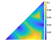
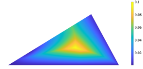
Refer to caption
(a) Square lattice TE mode
Refer to caption
(b) Hexagonal lattice TE mode
Figure 6: Locations with distance between two adjacent band functions below 0.010.010.01 are marked blue.

6.1 Numerical tests with square lattice in Figure 2

We first test Algorithm 2 on the square lattice with the TE mode and compare the performance of GPI with Fekete points and Chebyshev points of the second kind (Cheb2).
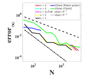
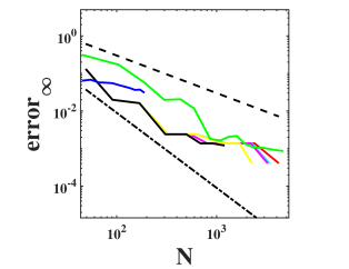
Refer to caption
(a) μ=1𝜇1\mu=1
Refer to caption
(b) μ=0.5𝜇0.5\mu=0.5
Figure 7: Maximum relative error with respect to the number of sampling points.

We present in Figure 7 the decay of errorsubscripterror\operatorname{error}_{\infty} against N𝑁N on a log-log scale of Algorithm 2 with κ{1,2,22,3,4}𝜅122234\kappa\in\{1,2,2\sqrt{2},3,4\} and μ{1,0.5}𝜇10.5\mu\in\{1,0.5\} as suggested in Remark 5.2. The performance of GPI with Fekete points and Cheb2 are also provided to facilitate comparison. Since Fekete points for polynomial spaces with (total) degrees higher than 18 are still unknown [30], GPI with Fekete points is restricted to N190𝑁190N\leq 190. We observe that Algorithm 2 outperforms GPI for all cases. Furthermore, an algebraic convergence rate between first order and second order is observed for any parameters of κ𝜅\kappa and μ𝜇\mu.

Refer to caption
(a) loop 2
Refer to caption
(b) loop 4
Refer to caption
(c) loop 6
Refer to caption
(d) loop 8
Refer to caption
(e) loop 2
Refer to caption
(f) loop 4
Refer to caption
(g) loop 6
Refer to caption
(h) loop 8
Figure 8: Algorithm 1 with κ=22𝜅22\kappa=2\sqrt{2} (the top row) and κ=2𝜅2\kappa=2 (the bottom row).

Figure 8 displays the adaptive meshes generated by Algorithm 1 with κ=22𝜅22\kappa=2\sqrt{2} and κ=2𝜅2\kappa=2, respectively. Comparing with Figure 6(a), one observes that Algorithm 1 adaptively refines the elements with crossings. Note that larger κ𝜅\kappa indicates more elements being marked and refined in each loop. The initial mesh has little effect on the resulting adaptive mesh since meshes overlap in the first several loops.
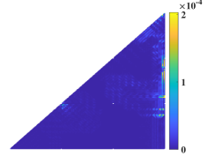
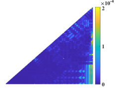
Refer to caption
(a) loop 8
Refer to caption
(b) loop 8
Figure 9: κ=22𝜅22\kappa=2\sqrt{2}: pointwise relative error ei(𝐤)subscript𝑒𝑖𝐤e_{i}(\mathbf{k}) under μ=1𝜇1\mu=1 (left), μ=0.5𝜇0.5\mu=0.5 (right).

Figures 9 and 10 display the pointwise relative error ei(𝐤)subscript𝑒𝑖𝐤e_{i}(\mathbf{k}) of approximating the first five band functions under κ=22𝜅22\kappa=2\sqrt{2} and κ=2𝜅2\kappa=2 and μ=1𝜇1\mu=1 and μ=0.5𝜇0.5\mu=0.5. Due to a lack of information about the seventh band function, we are unable to determine the positions of all the singular points of the sixth band function. Therefore, the error analysis only takes into account the first five band functions, even though we interpolate the first six band functions. From Figures 9(a) and 10(a), one observes that with μ=1𝜇1\mu=1 (i.e., the total polynomial degree on each element is consistent with its layer), the pointwise relative error ei(𝐤)subscript𝑒𝑖𝐤e_{i}(\mathbf{k}) dominates in the singular element patch 𝒯nSsuperscriptsubscript𝒯𝑛𝑆\mathcal{T}_{n}^{S} with n=8𝑛8n=8. This confirms Theorem 3.2, and (5.9). However, for a smaller slope parameter μ=0.5𝜇0.5\mu=0.5, the pointwise relative error ei(𝐤)subscript𝑒𝑖𝐤e_{i}(\mathbf{k}) in Figures 9(b) and 10(b) can take large values in the regular element patch 𝒯nRsuperscriptsubscript𝒯𝑛𝑅\mathcal{T}_{n}^{R} with n=8𝑛8n=8, indicating that the condition (5.9) fails.
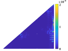
Refer to caption
(a) loop 8
Refer to caption
(b) loop 8
Figure 10: κ=2𝜅2\kappa=2: pointwise relative error ei(𝐤)subscript𝑒𝑖𝐤e_{i}(\mathbf{k}) under μ=1𝜇1\mu=1 (left), μ=0.5𝜇0.5\mu=0.5 (right).

6.2 Numerical tests with hexagonal lattice in Figure 3

Now we study 2D PhCs with infinite periodic hexagonal lattice, cf. Figure 3. The unit cell of the PhC is composed of six cylinders of dielectric material with dielectric constant ϵ=8.9italic-ϵ8.9\epsilon=8.9 embedded in the air and the lattice vectors 𝐚1=a4(e1+3e2)subscript𝐚1𝑎4subscript𝑒13subscript𝑒2\mathbf{a}_{1}=\frac{a}{4}({e}_{1}+\sqrt{3}{e}_{2}) and 𝐚2=a4(e13e2)subscript𝐚2𝑎4subscript𝑒13subscript𝑒2\mathbf{a}_{2}=\frac{a}{4}({e}_{1}-\sqrt{3}{e}_{2}) with lattice constant a=3R𝑎3𝑅a=3R, R𝑅R is the length of hexagon edges and r=13R𝑟13𝑅r=\frac{1}{3}R is the radius of cylinders. We observe similar results as before. Figure 11 shows the log-log plot of errorsubscripterror\operatorname{error}_{\infty} against N𝑁N. The adaptive mesh generated by Algorithm 1 and pointwise relative errors ei(𝐤)subscripte𝑖𝐤\operatorname{e}_{i}(\mathbf{k}) with κ=2,22𝜅222\kappa=2,2\sqrt{2}, μ=0.5,1𝜇0.51\mu=0.5,1 are displayed in Figures 12, 13, 14, demonstrating the efficiency and reliability of Algorithm 2.
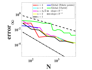
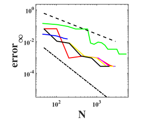
Refer to caption
(a) μ=1𝜇1\mu=1
Refer to caption
(b) μ=0.5𝜇0.5\mu=0.5
Figure 11: Maximum relative error with respect to the number of sampling points.
Refer to caption
(a) loop 2
Refer to caption
(b) loop 4
Refer to caption
(c) loop 6
Refer to caption
(d) loop 8
Refer to caption
(e) loop 2
Refer to caption
(f) loop 4
Refer to caption
(g) loop 6
Refer to caption
(h) loop 8
Figure 12: Algorithm 1 with κ=22𝜅22\kappa=2\sqrt{2} (the top row) and κ=2𝜅2\kappa=2 (the bottom row).
Refer to caption
(a) loop 8
Refer to caption
(b) loop 8
Figure 13: κ=22𝜅22\kappa=2\sqrt{2}: pointwise relative error ei(𝐤)subscript𝑒𝑖𝐤e_{i}(\mathbf{k}) under μ=1𝜇1\mu=1 (left), μ=0.5𝜇0.5\mu=0.5 (right).
Refer to caption
(a) loop 8
Refer to caption
(b) loop 8
Figure 14: κ=2𝜅2\kappa=2: pointwise relative error ei(𝐤)subscript𝑒𝑖𝐤e_{i}(\mathbf{k}) under μ=1𝜇1\mu=1 (left), μ=0.5𝜇0.5\mu=0.5 (right).

7 Conclusion

In this work, we have presented an hp𝑝hp-adaptive sampling algorithm that can accurately approximate the band functions for two-dimensional photonic crystals. In the algorithm, we first generate an adaptive mesh that can refine elements containing singular points, and then assign proper polynomial degrees to each element based on its level. Additionally, we assign proper polynomial degrees to each edge to ensure a continuous global polynomial space. Finally, we develop an element-wise interpolation scheme using the global polynomial space to approximate band functions. We proved a first-order convergence rate in the worst-case scenario and presented several numerical tests to verify its performance. One interesting future research question is about approximating three-dimensional band functions, which is highly nontrivial due to a lack of provable local polynomial interpolation method on a tetrahedral domain. We plan to research on designing an optimal 3D PhCs with a maximum band gap.

References

  • [1] M. Ainsworth and T. Oden. A posteriori error estimation in finite element analysis. Comput. Methods Appl. Mech. Eng., 142(1-2):1–88, 1997.
  • [2] I. Babuška and M. Suri. The p𝑝p and hh-p𝑝p versions of the finite element method, basic principles and properties. SIAM Rev., 36(4):578–632, 1994.
  • [3] G. Bao, L. Cowsar, and W. Masters, editors. Mathematical modeling in optical science. SIAM, Philadelphia, PA, 2001.
  • [4] P. Binev, W. Dahmen, and R. DeVore. Adaptive finite element methods with convergence rates. Numerische Mathematik, 97:219–268, 2004.
  • [5] C. Canuto, M. Y. Hussaini, A. Quarteroni, and T. A. Zang. Spectral methods. Springer-Verlag, Berlin, 2006. Fundamentals in single domains.
  • [6] P. G. Ciarlet. The finite element method for elliptic problems. SIAM, Philadelphia, PA, 2002.
  • [7] L. Dong, A. Mckay, A. Marcinkevicius, L. Fu, J. Li, K. Thomas, and E. Fermann. Extending effective area of fundamental mode in optical fibers. J. Lightwave Technol., 27(11):1565–1570, 2009.
  • [8] V. K. Dzyadyk and I. A. Shevchuk. Theory of uniform approximation of functions by polynomials. Walter de Gruyter GmbH & Co. KG, Berlin, 2008.
  • [9] T. Eidam, J. Rothhardt, F. Stutzki, F. Jansen, S. Hädrich, H. Carstens, C. Jauregui, J. Limpert, and A. Tünnermann. Fiber chirped-pulse amplification system emitting 3.8 GW peak power. Optics Express, 19(1):255–260, 2011.
  • [10] L. Fejér. Bestimmung derjenigen Abszissen eines Intervalles, für welche die Quadratsumme der Grundfunktionen der Lagrangeschen Interpolation im Intervalle ein möglichst kleines Maximum besitzt. Annali della Scuola Normale Superiore di Pisa-Classe di Scienze, 1(3):263–276, 1932.
  • [11] S. Funken, D. Praetorius, and P. Wissgott. Efficient implementation of adaptive P1-FEM in Matlab. Comput. Methods Appl. Math., 11(4):460–490, 2011.
  • [12] J. Gilewicz, V. Kryakin, and A. Shevchuk. Boundedness by 3 of the Whitney interpolation constant. J. Approx. Theory, 119(2):271–290, 2002.
  • [13] D. Hermann, M. Frank, K. Busch, and P. Wölfle. Photonic band structure computations. Optics Express, 8(3):167–172, 2001.
  • [14] Y. Hinuma, G. Pizzi, Y. Kumagai, F. Oba, and I. Tanaka. Band structure diagram paths based on crystallography. Comput. Mater. Sci., 128:140–184, 2017.
  • [15] D. Jackson. Classical electrodynamics. Wiley, New York, 1999.
  • [16] J. Joannopoulos, S. Johnson, J. Winn, and R. Meade. Molding the flow of light. Princeton Univ. Press, Princeton, NJ, 2008.
  • [17] H. Johnen and K. Scherer. On the equivalence of the k-functional and moduli of continuity and some applications. In Constructive Theory of Functions of Several Variables: Proceedings of a Conference Held at Oberwolfach April 25–May 1, 1976, pages 119–140. Springer, 2006.
  • [18] M. Kadec. On the distribution of points of maximum deviation in the approximation of continuous functions by polynomials. Amer. Math. Soc. Transl.(2), 26:231–234, 1963.
  • [19] B. Karaivanov and P. Petrushev. Nonlinear piecewise polynomial approximation beyond Besov spaces. Appl. Comput. Harm. Anal., 15(3):177–223, 2003.
  • [20] C. Kittel. Introduction to solid state physics. John Wiley & Sons, USA, 2018.
  • [21] V. Kryakin. On exact constants in the Whitney theorem. Math. Notes, 54(1):688–700, 1993.
  • [22] P. Kuchment. Floquet Theory for Partial Differential Equations. Birkhäuser Verlag, Basel, 1993.
  • [23] D. Labilloy, H. Benisty, C. Weisbuch, T. Krauss, V. Bardinal, and U. Oesterle. Demonstration of cavity mode between two-dimensional photonic-crystal mirrors. Electronics Letters, 33(23):1978–1980, 1997.
  • [24] J. M. Melenk. hp𝑝hp-finite element methods for singular perturbations. Springer-Verlag, Berlin, 2002.
  • [25] P.-O. Persson and G. Strang. A simple mesh generator in MATLAB. SIAM Rev., 46(2):329–345, 2004.
  • [26] P. Russell. Photonic crystal fibers. Science, 299(5605):358–362, 2003.
  • [27] C. Schwab. p𝑝p- and hp𝑝hp-finite element methods. The Clarendon Press, Oxford University Press, New York, 1998. Theory and applications in solid and fluid mechanics.
  • [28] B. H. Sendov and M. D. Takev. A theorem of Whitney’s type in 𝐑2superscript𝐑2{\bf R}^{2}. Pliska Stud. Math. Bulgar., 11(1):78–85, 1991.
  • [29] B. Sündermann. Lebesgue constants in Lagrangian interpolation at the Fekete points. Mitt. Math. Ges. Hamburg, 11(2):204–211, 1983.
  • [30] A. Taylor, A. Wingate, and E. Vincent. An algorithm for computing Fekete points in the triangle. SIAM J. Numer. Anal., 38(5):1707–1720, 2000.
  • [31] A. F. Timan. Theory of approximation of functions of a real variable. Dover Publications, Inc., New York, 1994. Translated from the Russian by J. Berry, Translation edited and with a preface by J. Cossar, Reprint of the 1963 English translation.
  • [32] C. T. Traxler. An algorithm for adaptive mesh refinement in n dimensions. Computing, 59:115–137, 1997.
  • [33] S. Wang, S. Li, and Y.-S. Wu. An analytical solution of pressure and displacement induced by recovery of poroelastic reservoirs and its applications. SPE Journal, 28(03):1329–1348, 2023.
  • [34] Y. Wang and G. Li. Dispersion relation reconstruction for 2D photonic crystals based on polynomial interpolation. To appear, J.Comput. Phys., 2023.
  • [35] R. Wilhelmsen. A Markov inequality in several dimensions. J. Approx. Theory, 11(3):216–220, 1974.
  • [36] F. Yanik, S. Fan, M. Soljačić, and D. Joannopoulos. All-optical transistor action with bistable switching in a photonic crystal cross-waveguide geometry. Optics letters, 28(24):2506–2508, 2003.