CLAP: Contrastive Learning with Augmented Prompts
for Robustness on Pretrained Vision-Language Models

Abstract

Contrastive vision-language models, e.g., CLIP, have garnered substantial attention for their exceptional generalization capabilities. However, their robustness to perturbations has ignited concerns. Existing strategies typically reinforce their resilience against adversarial examples by enabling the image encoder to ”see” these perturbed examples, often necessitating a complete retraining of the image encoder on both natural and adversarial samples.

In this study, we propose a new method to enhance robustness solely through text augmentation, eliminating the need for retraining the image encoder on adversarial examples. Our motivation arises from the realization that text and image data inherently occupy a shared latent space, comprising latent content variables and style variables. This insight suggests the feasibility of learning to disentangle these latent content variables using text data exclusively. To accomplish this, we introduce an effective text augmentation method that focuses on modifying the style while preserving the content in the text data. By changing the style part of the text data, we empower the text encoder to emphasize latent content variables, ultimately enhancing the robustness of vision-language models. Our experiments across various datasets demonstrate substantial improvements in the robustness of the pre-trained CLIP model.

1 Introduction

Vision-language models pretrained with the InfoNCE loss [24], exemplified by models like CLIP [26] and ALIGN [14], have garnered considerable attention for their remarkable zero-shot capabilities, particularly in scenarios where extensive image-text pairings are available. However, it has been observed that the effectiveness of these models in zero-shot situations is heavily contingent on the input text prompts [37, 15], raising concerns about the robustness of CLIP-like models.

To address the concern above, efforts have focused on enhancing the robustness of CLIP through adaptation [22] or fine-tuning [34, 32]. A brief review for related work is provided in Sec. 2. However, these methods typically exhibit two main disadvantages. First, they are designed to address specific attacks, enhancing the robustness of CLIP by exposing it to particular generated adversarial examples. Consequently, when confronted with unknown or unobserved adversarial attacks, these methods may face significant challenges. This challenge becomes even more pronounced in the face of the fact that we cannot foresee and provide defenses for all attack scenarios. Second, current approaches to enable CLIP to understand and incorporate these adversarial samples, require significant computational resources, which severely limits its applications.

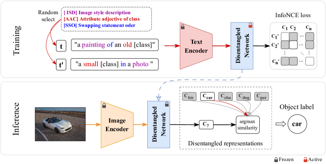
Figure 1: The CLAP (Contrastive Learning with Augmented Prompts) framework, based on a pretrained text encoder with fixed gradients, trains a disentangled network using augmented prompt pairs with the InfoNCE loss. After training, the disentangled network is positioned directly atop CLIP’s image encoder, boosting the robustness of representations in both zero-shot scenarios across various prompts and few-shot learning situations.

In contrast to the aforementioned methods, our approach does not need exhausting adversarial examples, nor heavy computation. The key of our approach to obtain robustness is exploring the underlying generative process of multi-modal data from a causal perspective. More specificially, we propose a causal generative model where both text and image data share a latent space. This latent space is divided into two subspaces, corresponding to latent content variables and latent style variables, respectively. We attribute the latent content variables cause object labels. To capture the correlation between latent style variables and object labels, we incorporate the notion that latent content variables causally influence latent style variables in our model. Additionally, acknowledging the asymmetry between image and text data, we posit distinct causal mechanisms for generating image and text data. Building upon the proposed causal generative model, our insight is that identifying content variables is crucial for significantly improving model robustness.

Current theories [30, 38] have demonstrated that utilizing sufficient changes in latent style variables can aid in identifying latent content variables through contrastive self-supervised learning. Typically, these methods rely on augmented image pairs to obtain the necessary changes. However, implementing augmentation to enable changes in all style variables is exceptionally challenging. For instance, transforming a photo of a dog into a sketch while maintaining the exact content but changing the style entirely is an extremely challenging task. In contrast, in the language modality, such a stylistic transformation can be easily accomplished by changing a phrase from ”a photo of a dog” to ”a sketch of a dog”. Building on this insight, we posit that introducing style variations through diverse augmented text data proves to be a more effective approach for ensuring sufficient changes in latent style variables. This, in turn, enhances the recovery of latent content variables, presenting a more effective strategy compared to relying solely on image data augmentation.

Inspired by the insights outlined above, we propose a novel method, termed CLAP (Contrastive Learning with Augmented Prompts), designed to attain disentangled and robust representations from pretrained vision-language models, as illustrated in Fig. 1. CLAP employs a contrastive loss to train a disentangled network atop CLIP’s text encoder, leveraging augmented prompt pairings. To ensure effective disentanglement, we have devised specific prompt augmentation techniques for text prompts and introduced an efficient residual MLP as the disentangled network. Comprehensive experiments across multiple datasets showcase CLAP’s efficacy, demonstrating robustness in zero-shot and few-shot scenarios, resilience to adversarial attacks, and potential in extracting content representations from CLIP’s overall representations.

In summary, we make the following contributions:

(1) We introduce a causal generative model that elucidates the generative process of image-text data, wherein the sensory aspects of both image and text data are captured in a shared latent space, divided into latent content variables and latent style variables.

(2) Motivated by the proposed generative model, we introduce CLAP, an innovative Contrastive Learning approach utilizing Augmented Prompts. CLAP aims to learn representations from pretrained vision-language models, approximating the true latent content variables. This approach demonstrates robustness, with low computational resource requirements and without relying on adversarial image examples.

(3) We propose a simple yet effective implementation for CLAP by introducing a residual MLP network with a zero-initialized projection. Our experiments on various natural datasets and their adversarial versions demonstrate the significant robustness of CLAP compared to CLIP, in terms of test accuracy.

2 Related work

Contrastive vision-language pretraining. Contrastive learning has proven successful in self-supervised models [5, 12, 13] by maximizing agreement between different augmented views of the same example and minimizing agreement among different examples. Extending beyond self-supervised learning, CLIP [26] pioneered the first large-scale contrastive vision-language model by leveraging an extensive collection of image-text pairs from the internet, showcasing remarkable zero-shot capabilities across diverse computer vision benchmarks. ALIGN [14] took this further by scaling up the training set of pretrained vision-language models to an astonishing one billion image-text pairs. Thanks to the vast scale of its cross-modal training data and the self-attention operations of the vision transformer [8], these contrastive vision-language models generalize well to various datasets and have become foundational models for numerous downstream tasks [28].

Robustness of vision-language models. The concept of model robustness is multifaceted. In terms of generalizing to ”unseen” datasets, CLIP-like models perform admirably due to their extensive training datasets. However, CLIP has shown sensitivity to the choice of input text prompts [37, 15], resulting in significant performance variance with different prompts. Recent research in response to CLIP-like models’ prompt sensitivity focuses on prompt learning or engineering [37, 15, 6, 36, 10] to tailor prompts for specific downstream tasks, yet this does not directly address the inherent robustness of CLIP’s representations. Additionally, CLIP-like models are susceptible to adversarial attacks [3, 9]. Current methods [22, 34] adapt the pretrained encoder using adversarially augmented image pairs to mitigate this. Unlike these approaches, our work aims to enhance CLIP’s robustness from a broader perspective, employing an image-free training approach without modifying its pretrained image encoder.

Disentangled representation learning. Disentangled Representation Learning aims to unravel underlying factors concealed within observable data in representation form [33, 29, 18], offering advantages for various applications through controllable and robust representations. Zimmermann et al. [38] suggest that contrastive learning may reverse the data generation process under certain conditions. Von Kügelgen et al. [30] propose that data augmentation can assist in segregating the content variable from the latent space. Different from these works, our work employs contrastive learning with augmented text data in an effort to achieve disentanglement.

3 Methods

To better comprehend the reasons for the robustness issues with CLIP, we formulate a causal generative model for image-text data, detailed in Section 3.1. Motivated by this model, we posit that identifying latent content variables offers an ideal solution for enhancing robustness. Fortunately, previous research has demonstrated that contrastive learning with image data augmentation provably isolates latent content variables from latent style variables in theory [30]. Building on the insight that introducing style variations through diverse augmented text data is a more effective strategy for ensuring substantial changes in latent style variables compared to image augmentation, we introduce CLAP in Section 3.2. Finally, in Section 3.3, we illustrate how to implement CLAP in a simple yet effective manner using a designed residual MLP network.

3.1 The proposed causal generative model

To improve the robustness of CLIP from the perspective of the underlying data generative process, we propose a causal generative model where image-text data stem from a shared latent space, as shown in Fig. 2.

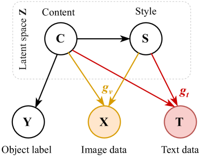
Figure 2: Image and text data are generated through separated deterministic processes, $\mathbf{g}_{v}$ for images and $\mathbf{g_{t}}$ for texts, from a shared latent space Z. This space consists of a content variable C and a style variable S. Both content and style variables contribute to creating multi-modal data, while the content variable alone determines the object’s label.

In the proposed model, the shared latent place is divided into two susbspaces, corresponding to latent content variables $\mathbf{C}$ and latent style variables $\mathbf{S}$, respectively. We attribute the latent content variables cause object labels $\mathbf{Y}$, which has been verified in previous works [21, 16, 19]. This represents the process where experts extract content information from provided images and subsequently assign appropriate labels based on their domain knowledge. To capture the correlation between latent style variables $\mathbf{S}$ and object variables $\mathbf{Y}$, we incorporate the notion that latent content variables $\mathbf{C}$ causally influence latent style variables $\mathbf{S}$ in our model. This is aligned with previous works in causal representation learning [30, 7, 19]. Additionally, considering the asymmetry between image and text data, where information in image data is typically much more abundant than in text data, we posit distinct causal mechanisms for generating image (i.e., $\mathbf{g_{v}}$) and text data (i.e., $\mathbf{g_{t}}$). Our generative model is formulated as follows:

$$\mathbf{S}:=\mathbf{g_{s}}(\mathbf{C}),$$ (1)

$$\mathbf{X}:=\mathbf{g_{v}}(\mathbf{C},\mathbf{S}),~{}\mathbf{T}:=\mathbf{g_{t}}(\mathbf{C},\mathbf{S}),~{}\mathbf{Y}:=\mathbf{g_{y}}(\mathbf{C}),$$ (2)

where $\mathbf{X}$ and $\mathbf{T}$ symbolize vision-modal and language-modal data, respectively, which are causally generated by the latent variables $\mathbf{C}$ and $\mathbf{S}$ through distinct causal mechanisms, represented as $\mathbf{g_{v}}$ for image data and $\mathbf{g_{t}}$ for text data. The label $\mathbf{Y}$ of an object is solely determined by $\mathbf{C}$ through $\mathbf{g_{y}}$.

Building on our proposed causal generative model, we argue that enhancing the disentanglement of the latent content variables is essential for significantly improving robustness. Recent significant work in [30] has demonstrated that the latent content variables can be identified up to block identifiability, by allowing all latent style variables to change. Such change can be done through augmentation on image. However, implementing augmentation to enable changes in all style variables is exceptionally challenging, as we highlighted in Introduction.

3.2 Contrastive learning with augmented prompts

Instead of using augmentation on image to enable latent style variables to change, we observed that stylistic transformations are more easily achieved in the language modality compared to the vision modality. This observation is rooted in the inherently logical structure and higher semantic level of text data over images. For instance, while transforming a photo of a dog into a sketch without altering its content poses a challenge, this transformation is readily achieved in text data by simply changing the phrase from ”a photo of a dog” to ”a sketch of a dog”. Therefore, in contrast to previous work [30] relying on augmented image pairs, we have chosen to utilize prompt augmentations as part of our contrastive learning approach.

Prompt augmentations. To achieve stylistic changes in text prompts without modifying their content, we’ve crafted specific data augmentation techniques for text, inspired by Wei and Zou [31]. Differing from their method, our prompt augmentations exclude random word insertions or deletions. This decision is due to the typically concise and fixed nature of text prompts, where random modifications could unintentionally change the content by either eliminating class names or adding new objects. our customized prompt augmentation methods, aimed at implementing style changes, are outlined as follows:

• ISD (Image Style Descriptions): This method is specifically crafted for augmenting descriptions of image styles.

• SRC (Synonyms Replacement of Class Names): This technique focuses on replacing class names with their synonyms.

• AAC (Attribute Adjectives of Class Names): Aimed at augmenting attribute adjectives related to class names.

• SSO (Swapping Statement Order): This approach is designed to rearrange the order of statements within prompts.

Specifically, for augmenting image style descriptions, we employ 13 descriptors for common image types, including ”painting”, ”sketch”, ”artistic depiction”, ”quick draw”, ”line drawing”, ”watercolor”, ”cartoon”, ”clipart”, ”image without background”, ”product image”, ”real-world image”, ”photo”, and ”infograph”. For synonyms of class names, we utilize WordNet [23] to find appropriate synonyms, manually filtering out any that are not contextually fitting. In the case of attributive adjectives, we use ChatGPT-3.5 [2] to produce a list of 50 adjectives that frequently describe visible attributes of objects, such as size, color, surface, pattern, and condition. We then select 42 words from this list, ensuring the exclusion of ambiguous terms. To provide a clearer understanding, we showcase examples of these prompt augmentation techniques in Tab. 1. For more detailed information on our prompt augmentation methods, please refer to Appendix B.

Augmentations	Prompt 1	Prompt 2
SRC	a bike	a bicycle
ISD	a photo of a bike	a cartoon of a bike
AAC	a red bike	a yellow bike
SSO	a bike in a photo	a photo of a bike

Table 1: Prompt augmentations with the class name ”bike.”

Learning objective. Aligned with the established objective of contrastive learning [38, 30, 5], we employ InfoNCE [24] as our loss function. We chose InfoNCE for its ability to effectively lower bound mutual information across similar views by enhancing the similarity of positive pairs while reducing similarity among negative pairs. The formula for the InfoNCE loss is structured as follows:

$$\mathop{\mathcal{L}}\limits_{\mathrm{\mathbf{f};\tau,K}}=\mathop{\mathbb{E}}\limits_{\{\mathbf{t}_{i}\}_{i=1}^{K}}[-\sum\limits_{i=1}^{K}\log\frac{\mathrm{exp}(\mathbf{\tilde{c}}_{i}\cdot\mathbf{\tilde{c}}^{\prime}_{i}/\tau)}{\sum\nolimits_{j=1}^{K}\mathrm{exp}(\mathbf{\tilde{c}}_{i}\cdot\mathbf{\tilde{c}}^{\prime}_{j}/\tau)}].$$ (3)

In the formula, $\mathbf{\tilde{c}}_{i}$ and $\mathbf{\tilde{c}^{\prime}}_{i}$ represent the L2-normalized representations, specifically $\mathbf{f}\circ\mathbf{f_{t}}(\tilde{\mathbf{t}}_{i})$ and $\mathbf{f}\circ\mathbf{f_{t}}(\tilde{\mathbf{t}}_{i}^{\prime})$, corresponding to distinct augmented texts of the $i$-th input prompt $\mathbf{t}_{i}$. Here, $\mathbf{f_{t}}$ denotes the fixed pretrained text encoder used during training, $\mathbf{f}$ is the disentangled network being trained, $\tau$ signifies a temperature parameter, and $K\!-\!1$ represents the number of negative prompt pairs.

Identifiability of the proposed causal model. With invertible generation function $\mathbf{g_{v}}$, the latent variables $\mathbf{C}$ can be identified up to block identifiability when sufficient augmentation is applied on the image data [30]. In our model, under the assumption that text data and image data share the same latent space, the text data can be used as a proxy for augmentations on images, i.e. we can indirectly augment image via augmenting text data. Thus based on Von Kügelgen et al. [30], prompt augmentations can also help to disentangle latent content and style from observational data.

3.3 Implementation with a disentangled network

In order to leverage the full benefits of the pretrained encoders, our approach is to initiate the optimization from the pretrained feature space, instead of beginning randomly. This led us to develop a residual MLP with a zero-initialized projection for our disentangled network, motivated by the zero-conv operation used in ControlNet [35]. In contrast to the zero-conv operation, we specifically employ a zero-linear operation in our network, as depicted in Fig. 3.

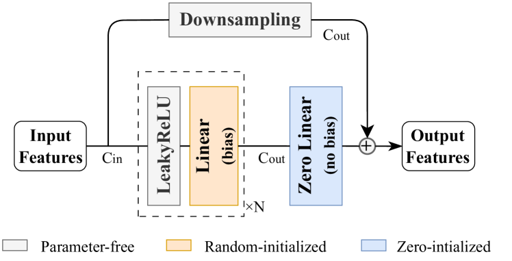
Figure 3: The disentangled network’s architecture. Key features include a residual block with a zero-initialized, bias-free linear layer acting as a projection for initiating optimization from the pretrained feature space. A downsampling function is applied to ensure aligning when input size $\mathrm{C_{in}}$ and output size $\mathrm{C_{out}}$ differ.

Unlike the original ControlNet, our disentangled network is built atop a fixed encoder and does not incorporate a trainable copy of the pretrained encoder or utilize an input condition. We have designed it with a residual block that includes a zero-initialized, bias-free linear layer positioned after a basic MLP consisting of $N$ repetitions of LeakyReLU-Linear layers. This zero-initialized linear layer serves as a projection, allowing the optimization process to initiate from the pretrained feature space instead of starting arbitrarily. Additionally, in cases of downsampling, our implementation employs nearest-neighbor interpolation to align features during changes in output size, ensuring the preservation of input feature sharpness.

Inference. After training, the disentangled network is directly integrated with CLIP’s image encoder for extracting content representations. This integration facilitates robust performance, both in zero-shot scenarios across various prompts and in few-shot learning situations.

4 Experiments

4.1 Implementation details

We implement CLAP on the ViT-B/16 model, pretrained with CLIP. Our experiments are conducted on a single NVIDIA RTX 3090 GPU.

Datasets. To evaluate the robustness of disentangled representations, we conduct experiments on three diverse multi-domain datasets: PACS [17] (4 domains, 7 classes), VLCS [1] (4 domains, 5 classes), and OfficeHome [27] (4 domains, 65 classes). Unlike traditional domain generalization evaluations, these datasets are chosen for their varied environmental settings to test the robustness of representations of CLAP. For ease of reference, we treat each domain within these datasets as a separate dataset.

Model. The output dimension of the disentangled network is set as the same of CLIP’s embeddings that is 512 for ViT-B/16, eliminating the need for downsampling of input features. The main branch comprises a leakyReLU-linear layer followed by a zero-initialized linear projection.

Training. We adjust the batch size to match the number of classes in each dataset, ensuring no class name repetition within a single batch: 7 for PACS, 5 for VLCS, and 65 for OfficeHome. Other hyper-parameters remain consistent across datasets. Our prompt augmentation strategy combines ”ISD+AAC+SSO”. We set the contrastive loss temperature $\tau$ at 0.1, using the Adam optimizer with a learning rate of 0.0001 and no weight decay. The total training steps are set to 100,000, with checkpoints every 50 steps to compute the average loss. Early stopping is triggered if the loss does not decrease by more than 0.001 for five consecutive checkpoints. We perform three training runs with different random seeds, reporting the average with standard deviation of the final weights’ performance.

Compute. CLAP achieves rapid convergence and short training durations. With pre-generated CLIP text representations, training on PACS converges in about 1.6 minutes at $916\pm 23$ steps, VLCS in roughly 1.5 minutes at $850\pm 81$ steps, and OfficeHome in approximately 10 minutes at $3530\pm 130$ steps.

4.2 Evaluations

To evaluate CLAP’s robustness, we perform three main experiments: zero-shot evaluation using different prompts, linear probes with text data for few-shot robustness, and adversarial attack tests to assess adversarial robustness.

In experiments with random operations, we use a consistent random seed for uniformity. For linear probes with text data, we use L2 normalization and cross-entropy loss in training, covering 1,000 epochs with a batch size of 128 and early stopping applied at a patience of 10 and a delta of $\delta=0.001$.

4.2.1 Zero-shot robustness across prompts

CLAP undergoes zero-shot evaluation using three different prompts: ”zs-C” (class names only), ”zs-PC” (using ”a photo of a [class name]”), and ”zs-CP” (with ”a [class name] in a photo”). As shown in Tab. 2, CLAP demonstrates notable uniformity across these prompts, evidenced by significantly reduced in standard deviation ($\delta$) and range ($R$), compared to CLIP’s original representations. This consistency underscores CLAP’s improved zero-shot robustness across various prompts.

		Average top-1 accuracy (%)
		CLIP						CLAP
Datasets		zs-C	zs-PC	zs-CP	Mean	$\delta(\downarrow)$	$R(\downarrow)$	zs-C	zs-PC	zs-CP	Mean	$\delta(\downarrow)$	$R(\downarrow)$
	ArtPainting	96.4	97.4	92.0	95.3	2.34	5.37	96.9±0.23	97.1±0.22	97.3±0.25	97.1	0.17	0.41
	Cartoon	98.9	99.1	98.3	98.7	0.32	0.77	98.6±0.21	98.6±0.10	98.9±0.07	98.7	0.17	0.39
	Photo	99.9	99.9	99.2	99.7	0.34	0.72	99.8±0.05	99.7±0.10	99.8±0.10	99.8	0.06	0.14
PACS	Sketch	87.7	88.2	83.5	86.5	2.08	4.63	91.9±0.17	91.8±0.16	92.0±0.30	91.9	0.13	0.31
	Caltech101	99.7	99.9	99.9	99.9	0.10	0.21	99.8±0.07	99.8±0.18	99.8±0.12	99.8	0.05	0.12
	LabelMe	61.8	70.2	69.8	67.2	3.88	8.43	67.5±2.80	68.3±2.84	67.8±2.96	67.9	0.35	0.82
	SUN09	70.1	73.6	73.4	72.4	1.57	3.41	67.1±2.83	65.2±2.83	66.2±2.81	66.2	0.81	1.93
VLCS	VOC2007	73.9	86.0	84.7	81.5	5.43	12.12	83.2±0.43	82.8±0.21	83.2±0.25	83.1	0.23	0.53
	Art	80.6	82.4	79.2	80.7	1.34	3.26	71.9±0.07	70.7±0.26	70.8±0.40	71.1	0.55	1.29
	Clipart	64.6	67.2	61.0	64.3	2.54	6.19	59.3±0.33	59.1±0.74	59.2±0.64	59.2	0.18	0.42
	Product	86.3	88.4	85.4	86.7	1.29	3.08	82.9±0.41	82.1±0.63	82.1±0.57	82.4	0.40	0.97
Off.Hom.	RealWorld	88.0	89.1	86.3	87.8	1.15	2.80	82.7±0.19	81.9±0.26	82.3±0.33	82.3	0.33	0.79

Table 2: Results of zero-shot with three distinct prompts. The significantly reduced standard deviations ($\delta$) and ranges ($R$) of accuracy compared to CLIP reveals that CLAP exhibits a notable improvement on zero-shot robustness across prompts.

Style information compromise CLIP’s zero-shot robustness across prompts. As shown in Tab. 2, CLIP consistently achieves its best performance with the ”PC” prompt on most datasets but shows notable performance drops with other prompts, particularly the ”CP” prompt. This tendency in CLIP likely stems from the predominance of the ”PC” (Photo of Class) pattern in its textual training data, leading to a lesser familiarity with ”CP” (Class in Photo) prompts. In contrast, thanks to better disentangled latent content variables, CLAP’s representations exhibit a marked decrease in this variance, showcasing improved zero-shot robustness across various prompts.

Upon a closer viewing of the results into dataset level, intriguing differences in mean accuracy between CLIP and CLAP are observed. In datasets like PACS Cartoon and VLCS Caltech101, where the label object (the object corresponding to an image’s label) dominates the image, CLAP outperforms CLIP. However, in datasets with smaller-scaled label objects such as VLCS SUN09 and OfficeHome Art, CLAP’s performance diminishes. Notably, in the PACS Sketch dataset, characterized by simple line drawings, CLAP significantly improves in accuracy. Fig. 4 features randomly selected samples from these datasets, demonstrating the varying pixel ratios occupied by the label object within each image.

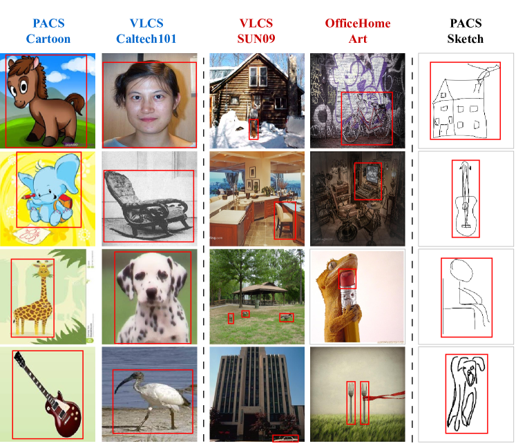
Figure 4: The object corresponding to an image’s label, marked by an red rectangle, differs across datasets. CLAP consistently shows robustness and excels in images with large-scaled or isolated objects, exemplified by PACS Cartoon, Sketch and VLCS Caltech101.

t-SNE Visualization. In our t-SNE visualizations, we compare CLIP’s representations with the disentangled representations of CLAP. As shown in Fig. 5, CLAP’s representations demonstrate a notable inter-class gap and a more cohesive intra-class convergence across various datasets. It is noteworthy that in cases with very small-scaled label objects, such as in SUN09, both CLIP and CLAP struggle to achieve clear separability between classes in terms of image labels. However, in datasets like PACS Sketch, characterized by simple line drawings, CLAP achieves clearer class differentiation. These visualizations underscore CLAP’s enhanced robustness and its more effective disentanglement of latent content variables in comparison to CLIP.

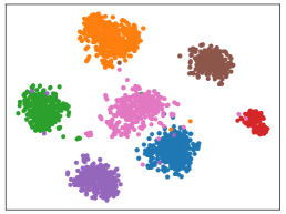
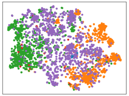
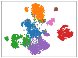
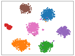
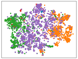
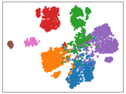
Figure 5: t-SNE visualization: The first row showcases visualizations of CLIP, while the second row presents CLAP. The datasets, from left to right, include PACS Cartoon, VLCS SUN09 and PACS Sketch.

4.2.2 Few-shot robustness

To assess robustness in few-shot learning and validate the disentanglement of content variables, CLAP undergoes a linear-probe evaluation using text data. Unlike image-based methods, which inherently include style information, our approach focuses on text data, allowing a clear contrast between training with only content information and training with both content and style. The evaluation includes 1-shot linear probes using text prompts with just the class name (lin.-C) and 13-shot probes with prompts combining class name and image style description (lin.-ISD). For concise reporting, we aggregate the average performance of datasets with the same name in Tab. 3, with more detailed results provided in Sec. A.1.

As shown in Tab. 3 and Fig. 6, CLAP’s performance closely aligns with its zero-shot capabilities in both 1-shot and 13-shot classifiers across all datasets, as indicated by minimal variations from zero-shot performance with the ”C” prompt to 13-shot ($\Delta_{\mathrm{ISD}}$) and 1-shot ($\Delta_{\mathrm{C}}$) performance. Notably, CLAP consistently outperforms CLIP in 1-shot scenarios (lin.-C) across all tested datasets. By contrast, CLIP’s performance fluctuates, showing a marked decrease in 1-shot scenarios with solely object information (lin.-C) and inconsistent outcomes in the 13-shot scenarios (lin.-ISD), with performance declines on the PACS datasets but improvements on others. These linear probe results underscore CLAP’s substantial few-shot robustness.

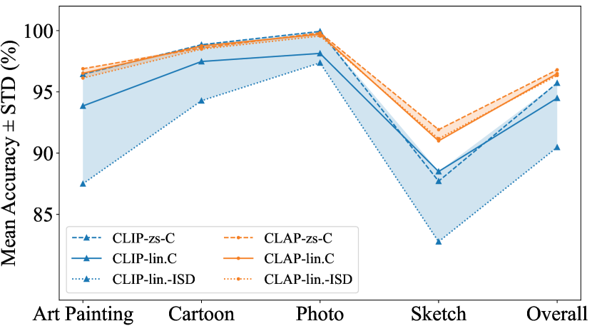
(a) PACS.

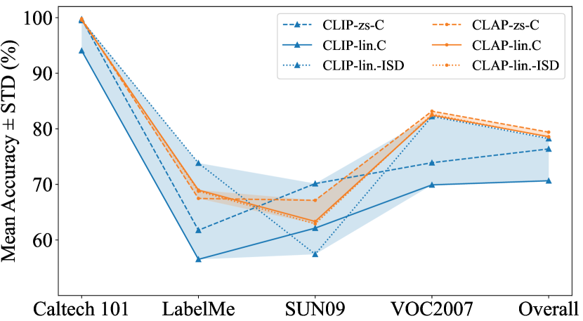
(b) VLCS.

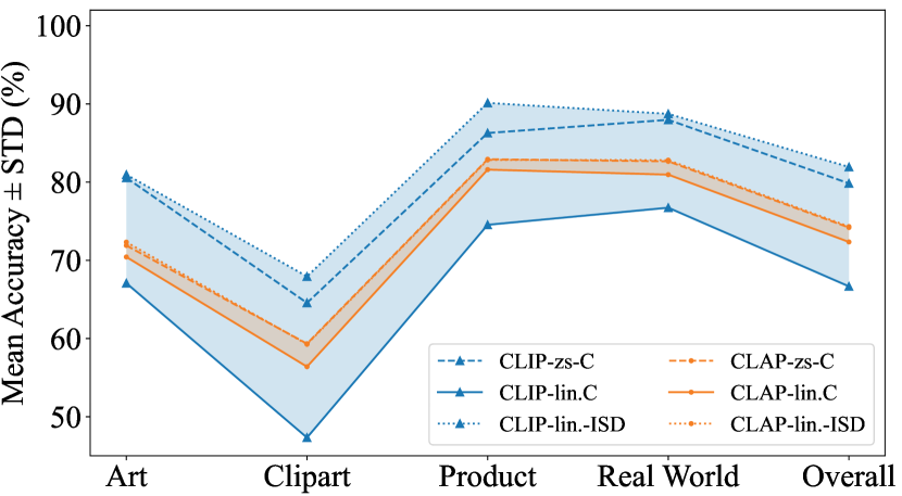
(c) OfficeHome.

Figure 6: Comparison of few-shot linear probes using text data reveals that CLIP experiences a notable decrease in performance in 1-shot scenarios using only class names (lin.-C). Conversely, CLAP’s performance closely matches its zero-shot results.

Style information detriments CLIP’s few-shot performance for isolated objects. CLAP demonstrates stable performance in few-shot linear probes with text data, regardless of whether style information is included in the training data, but CLIP shows variable outcomes. As depicted in Fig. 6, with smaller-scaled label objects (e.g., in OfficeHome datasets and VLCS’s LabelMe, VOC2007), style information enhances CLIP’s performance, with its 13-shot classifier (lin.-ISD) outperforming the 1-shot classifier (lin.-C). However, in cases of larger-scaled label objects, like in PACS (Art Painting, Cartoon, Sketch) and VLCS Caltech101, style information adversely affects CLIP’s performance, leading to the lowest results in the 13-shot classifier (lin.-ISD). This detrimental impact of style information is especially notable in datasets with isolated objects, such as PACS Sketch.

		Average top-1 accuracy (%)
Method		PACS	VLCS	OfficeHome
	CLIP	95.7±0.00	76.4±0.00	79.8±0.00
zs-C	CLAP	96.8±0.04	79.4±0.39	74.2±0.24
	CLIP	90.5±0.00	78.3±0.00	81.9±0.00
lin.-ISD	CLAP	96.3±0.07	78.5±0.67	74.3±0.70
	CLIP	94.5±0.00	70.7±0.00	66.7±0.00
lin.-C	CLAP	96.5±0.07	78.6±0.67	72.3±1.19
	CLIP	-5.3±0.00	1.9±0.00	2.1±0.00
$\Delta_{\mathrm{ISD}}(|\!\downarrow\!|)$	CLAP	-0.5±0.05	-0.9±0.66	0.1±0.51
	CLIP	-1.2±0.00	-5.7±0.00	-13.2±0.00
$\Delta_{\mathrm{C}}(|\!\downarrow\!|)$	CLAP	-0.3±0.03	-0.8±0.81	-1.9±0.95

Table 3: Results of few-shot learning robustness using only class names (1-shot) and prompts containing image style descriptions (13-shot).

4.2.3 Adversarial robustness

To assess CLAP’s enhanced adversarial robustness, we test the 1-shot classifiers (lin.-C) previously learned. We employ widely recognized adversarial attack methods, including FGSM [11], PGD [20] and CW [4], to generate adversarial samples. For FGSM, we implement 1 iteration, and for both PGD and CW, we apply 20 iterations, all with an $\epsilon$ of 0.031. As detailed in Tab. 4, the 1-shot classifier learned with CLAP’s representations exhibits significantly greater robustness to various adversarial attacks compared to the one trained with CLIP’s representations. This adversarial robustness is particularly pronounced in cases with large-scaled label objects, such as in PACS (Art Painting, Photo) and VLCS (Caltech101, VOC2007), as highlighted rows in Tab. 4.

		Average top-1 accuracy (%)
		Natural		FGSM		PGD-20		CW-20
Datasets		CLIP	CLAP	CLIP	CLAP	CLIP	CLAP	CLIP	CLAP
	A.	93.9	96.5	79.6	87.0	43.1	68.1	1.0	1.4
	C.	97.5	98.7	93.4	95.4	68.2	79.8	23.3	29.7
	P.	98.1	99.7	89.3	93.0	46.8	82.9	2.2	4.2
PACS	S.	88.5	91.0	84.7	88.8	74.9	78.5	73.9	76.6
	C.	94.1	99.6	93.7	97.7	18.9	91.2	3.4	5.7
	L.	56.5	69.0	52.6	56.8	15.6	26.5	0.2	0.4
	S.	62.1	63.3	53.3	53.0	4.3	16.0	0.0	0.3
VLCS	V.	69.9	82.4	60.4	72.1	19.5	42.3	1.1	2.3
	A.	67.1	70.4	39.8	44.1	16.6	17.2	2.1	1.2
	C.	47.3	56.4	34.3	42.3	17.7	18.5	7.9	7.8
	P.	74.5	81.6	49.5	56.1	21.9	24.0	5.3	6.1
Off.Hom.	R.	76.7	81.0	52.4	56.8	26.1	26.6	3.7	2.9

Table 4: Evaluation of 1-shot linear classifiers’ adversarial robustness, trained using only class names with CLIP and CLAP representations. CLAP consistently outperforms CLIP across datasets.

Additionally, We evaluate the zero-shot robustness of CLIP and CLAP against adversarial attacks using adversarial samples generated by corresponding 1-shot classifiers. Evaluating with ”C”, ”PC”, and ”CP” prompts, we find that CLAP retains its zero-shot robustness across various prompts. Its average accuracy, however, decreases in datasets with small-scaled label objects and significantly improves in scenarios featuring large-scaled or isolated objects. This pattern suggests CLIP’s dependence on style information and CLAP’s more effective disentanglement of content variables. Detailed results can be found in Sec. A.1.

Our evaluations show that CLAP significantly improves the robustness of pretrained vision-language models, confirming that better disentanglement of latent content variables leads to enhanced robustness. CLAP’s strong performance in scenarios with large-scaled or isolated objects also highlights its potential for object-centric tasks.

4.3 More analysis

Augmentation combinations. In Tab. 5, we explore different combinations of prompt augmentation methods on PACS datasets. Each combination shows effectiveness in disentangling content variables to some extent. The ”ISD+AAC+SSO” combination achieves the highest average accuracy, while using only ”ISD” or the ”ISD+SRC+AAC” combination leads to the smallest variation in standard deviation across prompts. For more detailed results, please refer to Sec. A.1.

	Average top-1 accuracy (%)
Prompt augmentations	zs-C	zs-PC	zs-CP	Mean	$\delta(\downarrow)$	$R(\downarrow)$
ISD	96.4	96.6	96.5	96.5	0.07	0.16
ISD+SRC	94.6	94.2	94.6	94.5	0.18	0.40
ISD+AAC	96.5	96.5	96.9	96.6	0.17	0.37
ISD+SSO	96.5	96.7	96.8	96.7	0.11	0.25
ISD+SRC+AAC	95.1	95.1	95.3	95.2	0.07	0.15
ISD+AAC+SSO	96.8	96.8	97.0	96.9	0.09	0.20
ISD+SRC+AAC+SSO	95.3	95.1	95.3	95.2	0.11	0.24

Table 5: Ablation study on different combinations of prompt augmentations.

Ablations. In Fig. 7, we evaluate the robustness in a zero-shot context using different prompts, comparing our specially designed residual MLP against a basic MLP of equivalent parameter size. We present the average accuracy along with the standard deviation for different prompts on PACS datasets. Our customized MLP consistently outperforms the basic MLP across all configurations of the output representation dimension $n_{dim}$ and the temperature $\tau$. Moreover, it demonstrates remarkable robustness across diverse prompts under all parameter settings. For a comprehensive analysis, detailed results can be found in Sec. A.1.

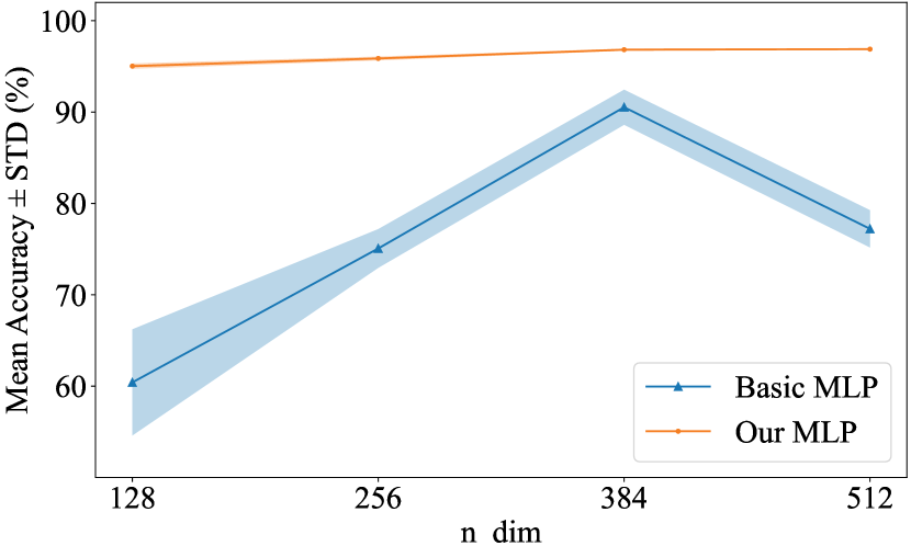
(a) Dimension of representations.

(b) $\tau$ in the contrastive loss.

Figure 7: Ablation study on $\tau$ and output dimension demonstrating the effectiveness of the devised disentangled detwork.

Experiments on ResNet50. We repeat our main experiments on ResNet50 pretrained with CLIP, similar results enhance our previous analysis. For more details, please refer to Sec. A.2.

Limitation. In our evaluation on the DomainNet dataset [25], which contains 345 classes, we observe a limitation in CLAP’s capacity to effectively develop robustness for this extensive dataset. This challenge appears to be linked to the limited range of stylistic transformations in our prompt augmentation techniques, particularly given the high number of class names. This shortfall restricts the generation of varied pairs that are crucial for successful contrastive learning. For more details on this experiment, please refer to Sec. A.3.

5 Conclusion

To bolster the robustness of pretrained contrastive vision-language models such as CLIP, this study delves into understanding the generative process of multi-modal data from a causal perspective. This exploration motivates a novel approach aimed at improving CLIP’s robustness by identifying latent content variables. Further, building on the insight that stylistic transformations are more readily achieved in the language modality than in the vision modality, we propose a method called Contrastive Learning with Augmented Prompts (CLAP). This approach, unlike relying on exhaustive adversarial examples or computationally intensive methods, focuses on enhancing robustness through a simple but effective contrastive learning with augmented prompts. Our extensive experiments affirm that CLAP significantly improves robustness, showcasing its effectiveness across various prompts, in few-shot learning scenarios, and in the face of adversarial attacks. We anticipate the application of CLAP in object-centric tasks and hope that our work inspires further investigations into disentangling latent variables within pretrained vision-language models.

Supplementary Material

Appendix A More experimental results

In this section, additional details about our experimental results are presented:

• Detailed results for CLIP pretrained ViT-B/16 are documented in Sec. A.1.

• We repeat our primary experiments on CLIP pretrained ResNet50x16 in Sec. A.2.

• Evaluations on the DomainNet dataset are elaborated in Sec. A.3.

A.1 Detailed experiment results on ViT-B/16

In Fig. 8, we showcase a comparison of the average top-1 accuracy and standard deviation for CLIP and CLAP across three unique prompts. These results highlight that CLAP consistently shows notably lower variance in zero-shot performance with various prompts across all evaluated datasets.

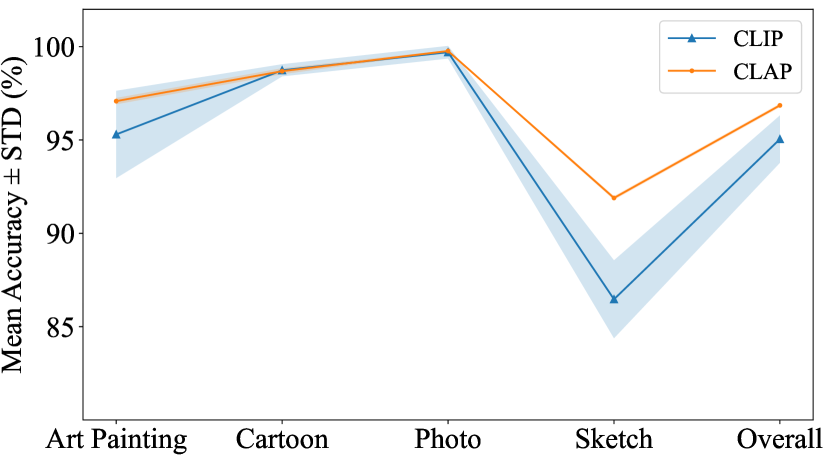
(a) PACS.

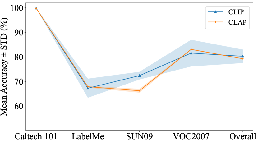
(b) VLCS.

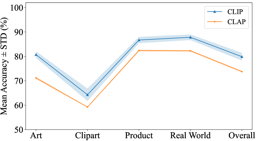
(c) OfficeHome.

Figure 8: Zero-Shot robustness across prompts. The solid line represents the average top-1 accuracy for each dataset in zero-shot scenarios, calculated across three distinct prompts. The shaded areas around the lines illustrate the standard deviations, emphasizing the performance variance across the prompts.

In Tab. 6, we present detailed results of the linear probe experiments using text data. Across all evaluated datasets, CLAP not only registers higher 1-shot (lin.-C) accuracy but also shows a significant reduction in variance from zero-shot to 13-shot ($\Delta_{\mathrm{lin.ISD}}$) and to 1-shot ($\Delta_{\mathrm{lin.C}}$). The results indicate that demonstrates enhanced in few-shot learning settings, utilizing both content-only and combined content-style information.

		Average top-1 accuracy (%)
		CLIP					CLAP
Datasets	Domains	zs-C	linear-ISD	linear-C	$\Delta_{\mathrm{ISD}}(\downarrow)$	$\Delta_{\mathrm{C}}(\downarrow)$	zs-C	linear-ISD	linear-C	$\Delta_{\mathrm{ISD}}(\downarrow)$	$\Delta_{\mathrm{C}}(\downarrow)$
	ArtPainting	96.4	87.5	93.9	-8.9	-2.6	96.9±0.23	96.1±0.23	96.5±0.44	-0.8±0.23	-0.4±0.30
	Cartoon	98.9	94.3	97.5	-4.6	-1.4	98.6±0.21	98.5±0.08	98.7±0.19	-0.1±0.26	0.2±0.19
	Photo	99.9	97.4	98.1	-2.6	-1.8	99.8±0.05	99.6±0.15	99.7±0.05	-0.3±0.10	-0.1±0.00
PACS	Sketch	87.7	82.8	88.5	-4.9	0.8	91.9±0.17	91.2±0.19	91.0±0.33	-0.7±0.15	-0.9±0.16
	Caltech101	99.7	99.5	94.1	-0.2	-5.7	99.8±0.07	99.7±0.19	99.6±0.33	-0.1±0.10	-0.3±0.27
	LabelMe	61.8	73.8	56.5	12.1	-5.2	67.5±2.80	68.8±2.46	69.0±1.83	1.3±1.45	1.5±1.18
	SUN09	70.1	57.4	62.1	-12.7	-8.0	67.1±2.28	62.9±3.00	63.3±3.43	-4.2±0.76	-3.8±1.31
VLCS	VOC2007	73.9	82.2	69.9	8.3	-4.0	83.2±0.43	82.6±0.32	82.4±0.26	-0.6±0.74	-0.7±0.67
	Art	80.6	81.0	67.1	0.4	-13.5	71.9±0.07	72.3±0.93	70.4±1.14	0.4±0.87	-1.5±1.08
	Clipart	64.6	67.9	47.3	3.4	-17.2	59.3±0.33	59.3±0.86	56.4±1.47	-0.1±0.53	-2.9±1.15
	Product	86.3	90.1	74.5	3.8	-11.7	82.9±0.41	82.8±0.69	81.6±1.32	-0.1±0.44	-1.3±1.01
Off.Hom.	RealWorld	88.0	88.7	76.7	0.8	-11.2	82.7±0.19	82.8±0.44	81.0±0.89	0.2±0.34	-1.7±0.70

Table 6: Detailed results of linear probes evaluation using text data. CLAP exhibits substantially improved few-shot robustness, as indicated by the changes from zero-shot with the ”C” prompt to 13-shot ($\Delta_{\mathrm{ISD}}$) and 1-shot ($\Delta_{\mathrm{C}}$) classifiers.

In Tab. 7, we report the results of zero-shot prediction under adversarial attacks which were applied to the 1-shot linear-C classifier. The results show that CLAP maintains consistent performance across different prompts, whereas CLIP’s features exhibit significant fluctuations.

In Tab. 8, detailed results for different augmentation combinations are presented. The findings highlight improved robustness achieved through contrastive learning with various combinations involving the ISD augmentation, where the ”ISD+AAC+SSO” combination exhibits the strongest performance on PACS datasets.

		Average top-1 accuracy of zero-shot (%)
		FGSM						PGD-20						CW-20
		CLIP			CLAP			CLIP			CLAP			CLIP			CLAP
Datasets	Domains	zs-C	zs-PC	zs-CP	zs-C	zs-PC	zs-CP	zs-C	zs-PC	zs-CP	zs-C	zs-PC	zs-CP	zs-C	zs-PC	zs-CP	zs-C	zs-PC	zs-CP
	A.	81.0	85.8	79.6	86.0	86.9	87.1	43.8	44.8	42.7	68.2	68.2	68.2	6.0	8.5	7.1	1.8	1.8	2.5
	C.	96.2	96.5	91.8	95.2	94.9	95.8	75.0	78.5	73.9	80.1	80.1	80.3	39.3	46.2	37.7	31.3	32.1	33.1
	P.	93.0	93.4	91.1	93.2	93.1	93.1	48.1	51.8	50.5	83.3	83.3	83.2	12.2	16.5	11.0	5.5	5.4	6.1
PACS	S.	84.5	85.6	78.2	88.8	88.5	89.1	76.4	77.7	73.2	79.5	79.3	79.7	75.7	76.9	66.9	77.0	76.9	77.4
	C.	98.9	98.7	98.7	98.3	98.4	98.3	37.4	54.8	50.3	91.0	91.0	91.0	24.2	41.9	38.0	7.1	6.7	6.7
	L.	50.9	56.5	60.2	54.9	54.2	54.4	17.5	17.7	18.0	26.5	26.5	26.5	3.5	4.3	4.4	0.8	0.8	0.8
	S.	57.3	65.0	66.7	56.4	55.1	55.9	5.7	6.0	6.9	16.0	16.0	16.0	2.4	2.5	3.3	0.4	0.3	0.3
VLCS	V.	66.9	74.7	74.9	72.7	72.6	72.9	21.2	23.2	23.2	42.1	42.0	42.0	7.1	10.8	9.9	3.2	3.4	3.4
	A.	57.8	56.7	54.6	46.8	46.4	46.9	19.3	19.9	19.4	18.1	17.9	18.1	6.4	7.3	6.7	2.5	2.2	2.4
	C.	50.0	51.8	42.9	44.6	44.9	45.0	24.4	25.3	22.9	20.4	20.5	20.7	16.9	17.5	15.5	10.3	10.4	10.8
	P.	63.3	65.8	59.4	58.3	58.1	58.7	28.2	29.0	28.1	25.3	25.2	25.4	15.7	16.8	15.7	8.5	8.3	8.5
Off.Hom.	R.	67.2	68.1	64.9	58.8	59.1	60.0	29.3	30.0	29.1	27.0	27.0	27.0	10.0	10.8	10.1	4.8	4.8	4.7

Table 7: Results from zero-shot predictions facing adversarial attacks on corresponding 1-shot classifiers show that CLAP maintains consistent zero-shot robustness across various prompts. It displays a notable improvement in accuracy in scenarios with large-scaled objects, but experiences a reduction in performance in other situations.

	ISD						ISD+SRC						ISD+AAC
PACS	zs-C	zs-PC	zs-CP	Mean	$\delta(\downarrow)$	$\mathbf{R}(\downarrow)$	zs-C	zs-PC	zs-CP	Mean	$\delta(\downarrow)$	$\mathbf{R}(\downarrow)$	zs-C	zs-PC	zs-CP	Mean	$\delta(\downarrow)$	$\mathbf{R}(\downarrow)$
A.	96.19	96.78	96.83	96.60	0.29	0.64	93.36	93.36	93.99	93.57	0.30	0.63	96.68	96.88	97.17	96.91	0.20	0.49
C.	97.65	97.74	97.53	97.64	0.09	0.21	96.12	95.61	95.69	95.81	0.22	0.51	98.08	98.25	98.72	98.35	0.27	0.64
P.	99.64	99.64	99.76	99.68	0.06	0.12	98.98	98.98	98.98	98.98	0.00	0.00	99.82	99.76	98.88	99.49	0.43	0.94
S.	92.08	92.06	92.01	92.05	0.03	0.07	90.05	88.95	89.74	89.58	0.46	1.10	91.50	91.09	91.65	91.41	0.24	0.56
Overall	96.39	96.55	96.53	96.49	0.07	0.16	94.63	94.23	94.60	94.49	0.18	0.40	96.52	96.49	96.86	96.62	0.17	0.37
	ISD+SRC+AAC						ISD+AAC+SSO						ISD+SRC+AAC+SSO
PACS	zs-C	zs-PC	zs-CP	Mean	$\delta(\downarrow)$	$\mathbf{R}(\downarrow)$	zs-C	zs-PC	zs-CP	Mean	$\delta(\downarrow)$	$\mathbf{R}(\downarrow)$	zs-C	zs-PC	zs-CP	Mean	$\delta(\downarrow)$	$\mathbf{R}(\downarrow)$
A.	96.44	96.24	96.63	96.44	0.16	0.39	97.22	97.36	97.66	97.41	0.18	0.44	96.44	96.24	96.63	96.44	0.16	0.39
C.	97.31	97.40	97.35	97.35	0.04	0.09	98.29	98.42	98.81	98.51	0.22	0.52	97.35	97.06	97.14	97.18	0.12	0.29
P.	99.28	99.52	99.34	99.38	0.10	0.24	99.82	99.76	99.88	99.82	0.05	0.12	99.22	99.40	99.28	99.30	0.07	0.18
S.	87.38	87.25	87.68	87.44	0.18	0.43	91.96	91.73	91.75	91.81	0.10	0.23	88.32	87.66	88.22	88.07	0.29	0.66
Overall	95.10	95.10	95.25	95.15	0.07	0.15	96.82	96.82	97.02	96.89	0.09	0.20	95.33	95.09	95.32	95.25	0.11	0.24
	ISD+SSO
PACS	zs-C	zs-PC	zs-CP	Mean	$\delta(\downarrow)$	$\mathbf{R}(\downarrow)$
A.	96.58	96.62	97.27	96.82	0.32	0.69
C.	97.40	97.87	97.70	97.66	0.19	0.47
P.	99.64	99.70	99.76	99.70	0.05	0.12
S.	92.44	92.39	92.34	92.39	0.04	0.10
Overall	96.52	96.72	96.77	96.67	0.11	0.25

Table 8: Detailed Results of experiments with various prompt augmentation combinations. All combinations incorporating the ISD augmentation enhance robustness to some extent. Notably, the combination of ”ISD+AAC+SSO” yields the best overall performance.

In Tab. 9 and Tab. 10, we provide the results of ablation studies on the PACS dataset, where we compare our custom-designed residual MLP with zero-initialized projection against a conventional MLP. These studies examine variations in the temperature parameter $\tau$ and the output dimension of disentangled representations. While the baseline MLP enhances CLIP’s robustness, our tailored MLP outperforms across all tested parameters, showing better performance and less variance among different values. This highlights the additional improvements afforded by our uniquely structured disentangled network.

		Average top-1 accuracy (%)
Structure	$\tau$	zs-C	zs-PC	zs-CP	Mean	$\delta(\downarrow)$	$R(\downarrow)$
	0.10	74.58	77.52	79.55	77.22	2.04	4.97
	0.20	90.58	91.90	92.07	91.52	0.67	1.49
	0.50	94.08	94.51	94.45	94.35	0.19	0.43
	1.00	94.44	94.87	94.79	94.70	0.19	0.43
Basic MLP	2.00	93.89	94.46	94.40	94.25	0.26	0.57
	0.10	96.82	96.82	97.02	96.89	0.09	0.20
	0.20	96.53	96.47	96.47	96.49	0.03	0.06
	0.50	96.51	96.46	96.42	96.46	0.04	0.09
	1.00	96.41	96.35	96.32	96.36	0.04	0.09
Our MLP	2.00	95.47	95.68	95.77	95.64	0.13	0.30

Table 9: Ablation study on the PACS dataset with varying temperature parameters ($\tau$).

		Average top-1 accuracy (%)
Structure	$n_{dim}$	zs-C	zs-PC	zs-CP	Mean	$\delta(\downarrow)$	$R(\downarrow)$
	128	56.30	56.30	68.62	60.41	5.81	12.32
	256	77.97	72.96	74.29	75.07	2.12	5.01
	384	87.82	91.71	92.06	90.53	1.92	4.24
Basic MLP	512	74.58	77.52	79.55	77.22	2.04	4.97
	128	94.62	95.30	95.17	95.03	0.29	0.68
	256	95.59	95.94	96.08	95.87	0.21	0.49
	384	96.72	96.80	96.98	96.83	0.11	0.26
Our MLP	512	96.82	96.82	97.02	96.89	0.09	0.20

Table 10: Ablation study on the PACS dataset with different output dimensions ($n_{dim}$).

A.2 Experiments on ResNet50x16

In this section, we elaborate on our repeated experiments utilizing the CLIP pretrained ResNet50 model. We specifically selected the ResNet50x16 variant and adjusted the output dimension to match its input dimension of 768. To ensure consistency and reproducibility across all randomized processes, we set the random seed to 2023. We maintain identical parameters to those used in the ViT-B/16 experiments, with comprehensive information available in Sec. 4.1.

Tab. 11 presents the zero-shot evaluation results for the ResNet50x16 model using three distinct prompts, in line with the protocol described in Sec. 4.2.1. These results confirm CLAP’s robustness in zero-shot scenarios across various prompts for the ResNet50x16 model. This is demonstrated by CLAP’s significantly lower standard deviations ($\delta$) and ranges ($R$) in accuracy across all tested datasets compared with CLIP.

		Average top-1 accuracy (%)
		CLIP						CLAP
Datasets		zs-C	zs-PC	zs-CP	Mean	$\delta$ (↓)	$R$ (↓)	zs-C	zs-PC	zs-CP	Mean	$\delta$ (↓)	$R$ (↓)
	ArtPainting	95.7	95.6	91.7	94.3	1.86	4.00	95.2	94.6	96.0	95.3	0.54	1.32
	Cartoon	98.3	98.6	97.5	98.1	0.44	1.06	97.8	97.5	98.1	97.8	0.24	0.59
	Photo	98.9	99.8	97.9	98.9	0.78	1.92	99.8	99.6	99.7	99.7	0.07	0.18
PACS	Sketch	91.5	91.9	84.1	89.2	3.59	7.81	92.3	92.6	92.6	92.5	0.13	0.29
	Caltech101	96.7	99.7	99.7	98.7	1.42	3.04	99.5	99.7	99.7	99.6	0.07	0.14
	LabelMe	53.4	59.4	51.6	54.8	3.33	7.79	58.6	58.9	57.5	58.3	0.59	1.36
	SUN09	63.2	72.8	67.8	67.9	3.95	9.66	72.2	72.1	72.8	72.4	0.29	0.64
VLCS	VOC2007	68.4	81.7	74.4	74.9	5.44	13.30	85.2	85.1	85.0	85.1	0.11	0.27
	Art	82.2	77.8	81.7	80.6	1.95	4.37	72.9	72.8	73.5	73.0	0.33	0.75
	Clipart	63.0	59.1	64.8	62.3	2.37	5.68	52.8	52.5	53.8	53.0	0.57	1.35
	Product	88.1	87.0	89.8	88.3	1.14	2.77	83.2	82.5	83.1	83.0	0.29	0.65
Off.Hom.	RealWorld	88.1	87.1	88.7	88.0	0.67	1.61	81.9	80.8	81.7	81.5	0.50	1.17

Table 11: CLAP’s zero-shot robustnesss across prompts holds for ResNet50x16 model variant, indicating by the notably reduced standard deviations ($\delta$) and ranges ($R$) of accuracy on all tested datasets compared to CLIP.

Tab. 12 showcases that CLAP’s few-shot performance on the ResNet50x16 model is consistent with its zero-shot performance for both 13-shot (lin.-ISD) and 1-shot (lin.-C) classifiers, as indicated by the small variances from zero-shot to 13-shot ($\Delta_{\mathrm{ISD}}$) and to 1-shot ($\Delta_{\mathrm{C}}$). These findings further confirm the few-shot robustness of the proposed method.

		Accuracy top-1 accuracy (%)
Method		PACS	VLCS	Off.Hom.
	CLIP	96.1	70.4	80.4
zs-C	CLAP	96.3	78.9	72.7
	CLIP	94.3	76.1	80.9
lin.-ISD	CLAP	96.0	77.9	72.7
	CLIP	94.9	69.9	63.5
lin.-C	CLAP	96.2	78.1	71.3
	CLIP	-1.8	5.6	0.5
$\Delta_{\mathrm{ISD}}(|\!\downarrow\!|)$	CLAP	-0.3	-1.0	0.0
	CLIP	-1.2	-0.5	-16.9
$\Delta_{\mathrm{C}}(|\!\downarrow\!|)$	CLAP	-0.1	-0.8	-1.4

Table 12: The few-shot robustness of CLAP for the ResNet50x16 model variant is confirmed by the considerably reduced variance ($\Delta_{\mathrm{ISD}}$) from zero-shot with the ”C” prompt (zs-C) to the 13-shot classifier (lin.-ISD), and the variance ($\Delta_{\mathrm{C}}$) from zs-C to the 1-shot classifier (lin.-C).

In Tab. 13, we present CLAP’s performance under three different adversarial attacks on its 1-shot classifier. The data illustrates CLAP’s enhanced robustness against FGSM and PGD-20 attacks on the majority of tested datasets, in comparison to CLIP. However, unlike the results observed with ViT-B/16, CLIP’s features appear to collapse under PGD-20 attacks in the ResNet50x16 model variant, as evidenced by the markedly low accuracy for both CLIP and CLAP’s 1-shot classifiers.

Datasets		Average top-1 accuracy (%)
		Natural		FGSM		PGD-20		CW-20
		CLIP	CLAP	CLIP	CLAP	CLIP	CLAP	CLIP	CLAP
PACS	A.	91.1	95.3	79.3	87.6	0.2	1.0	0.3	0.5
	C.	95.9	97.9	92.5	95.0	13.1	17.6	14.5	15.6
	P.	99.4	99.6	93.1	94.4	1.3	4.6	1.3	1.6
	S.	93.1	91.8	91.1	90.8	64.4	61.6	66.4	62.8
VLCS	C.	98.0	99.5	82.6	97.0	2.0	1.4	1.8	1.7
	L.	51.3	56.8	50.0	53.2	0.1	0.1	0.1	0.1
	S.	63.5	71.6	51.3	63.5	0.1	0.0	0.1	0.0
	V.	67.0	84.5	58.3	77.0	0.4	0.6	0.4	0.7
Off.Hom.	A.	61.5	71.1	46.4	51.7	1.0	2.1	1.2	1.2
	C.	48.6	52.6	36.7	39.2	6.2	5.6	6.0	5.1
	P.	72.1	81.1	52.1	60.4	5.7	5.4	5.5	4.0
	R.	71.7	80.6	55.5	60.7	2.9	4.7	2.8	2.4

Table 13: The adversarial robustness of CLAP is maintained for the ResNet50x16 model variant across most of the tested datasets.

A.3 Evaluation on the DomainNet dataset

Tab. 14 details our zero-shot evaluation results using the ViT-B/16 model on the DomainNet datasets. Here, the reduced standard deviations ($\delta$) and ranges ($R$) indicate an improvement in robustness across different prompts. However, significant differences between zero-shot and few-shot performances, as shown by $\Delta_{\mathrm{ISD}}$ and $\Delta_{\mathrm{lin.C}}$ in Tab. 15, point to CLAP’s challenges in effectively disentangling content variables in datasets with a wide array of classes, like DomainNet.

		Average top-1 accuracy on DomainNet(%)
Method		Clipart	Infograph	Painting	Quickdraw	Real	Sketch	Overall
	zs-C	70.97	48.60	66.62	14.91	82.58	63.03	57.78
	zs-PC	70.55	47.18	66.05	14.15	83.23	62.81	57.33
	zs-CP	68.91	46.06	65.08	12.26	81.33	59.45	55.51
	Mean	69.94	47.33	65.92	13.77	82.38	61.76	56.87
	$\delta$	1.03	1.27	0.64	1.11	0.79	1.64	0.98
CLIP	$R$	2.06	2.54	1.54	2.65	1.90	3.58	2.27
	zs-C	66.77±0.32	43.73±0.50	59.78±0.63	14.14±0.52	77.52±0.31	57.76±0.58	53.28±0.41
	zs-PC	66.75±0.49	42.89±0.75	60.20±0.73	14.09±0.39	78.06±0.40	58.12±0.59	53.35±0.54
	zs-CP	66.76±0.38	43.01±0.60	59.98±0.62	14.08±0.39	77.65±0.37	57.96±0.49	53.24±0.45
	Mean	66.76±0.38	43.21±0.62	59.99±0.66	14.10±0.43	77.74±0.36	57.95±0.55	53.29±0.46
	$\delta$	0.12±0.05	0.38±0.10	0.18±0.06	0.09±0.05	0.23±0.03	0.16±0.05	0.06±0.05
CLAP	$R$	0.28±0.12	0.87±0.23	0.42±0.15	0.21±0.11	0.54±0.09	0.36±0.09	0.13±0.09

Table 14: Zero-shot evaluation on the DomainNet dataset. The observed standard deviations ($\delta$) and ranges ($R$) suggest an improvement in robustness for zero-shot performance across different prompts.

		Average top-1 accuracy on DomainNet(%)
Method		Clipart	Infograph	Painting	Quickdraw	Real	Sketch	Overall
	zs-C	70.97	48.60	66.62	14.91	82.58	63.03	57.78
	linear-ISD	57.84	40.49	57.70	12.09	70.31	52.59	48.50
	linear-C	54.63	37.60	52.97	11.61	66.85	48.66	45.39
	$\Delta_{\mathrm{ISD}}(\downarrow)$	-13.13	-8.11	-8.92	-2.82	-12.27	-10.44	-9.28
CLIP	$\Delta_{\mathrm{C}}(\downarrow)$	-16.34	-11.00	-13.65	-3.30	-15.73	-14.37	-12.39
	zs-C	66.77±0.32	43.73±0.50	59.78±0.63	14.14±0.52	77.52±0.31	57.76±0.58	53.28±0.41
	linear-ISD	54.88±0.10	35.32±0.20	53.39±0.17	11.29±0.63	67.04±0.11	49.44±0.11	45.22±0.17
	linear-C	51.69±0.17	32.93±0.25	49.90±0.49	10.23±0.62	64.01±0.14	46.04±0.13	42.47±0.16
	$\Delta_{\mathrm{ISD}}(\downarrow)$	-11.89±0.39	-8.41±0.30	-6.39±0.47	-2.85±0.30	-10.48±0.31	-8.32±0.48	-8.06±0.35
CLAP	$\Delta_{\mathrm{C}}(\downarrow)$	-15.08±0.49	-10.80±0.32	-9.88±0.20	-3.91±0.30	-13.51±0.43	-11.72±0.44	-10.82±0.36

Table 15: Linear probes using text data on the DomainNet dataset. The marked differences between zero-shot and few-shot results, shown by $\Delta_{\mathrm{ISD}}$ and $\Delta_{\mathrm{C}}$, underscore the difficulties CLAP faces in improving robustness for datasets featuring a wide array of categories, such as DomainNet.

Appendix B Details on prompt augmentations

In this section, we provide more details on our prompt augmentation techniques. Tab. 16 includes detailed descriptions of the image styles and attributive adjectives used in our approach. Furthermore, In Tab. 17, we list the specific synonyms for class names from the PACS, VLCS, OfficeHome, and DomainNet datasets employed in our SRC augmentation. For succinctness, the table does not include class names without a synonym.

Aug.	Descriptions
ISD	painting, sketch, artistic depiction, photo,
	quick draw, line drawing, watercolor,
	cartoon, clipart, image without background,
	product image, real-world image, infograph
AAC	small, large, tiny, huge, compact, enormous,
	miniature, gigantic, petite, massive, red,
	blue, green, yellow, purple, orange, black,
	white, gray, pink, smooth, rough, shiny,
	matte, polished, textured, glossy, dull,
	lustrous, worn, new, old, cracked, pristine,
	tarnished, scratched, damaged, weathered,
	well-maintained, antique

Table 16: Descriptions of ISD (image style decriptions) and AAC (attributive adjectives of class names) augmentations in the proposed method.

Name	Synonyms	Name	Synonyms	Name	Synonyms
bird	fowl	firetruck	fire truck,fire engine	cooler	ice chest
car	auto, automobile, machine, motocar	flashlight	torch	cow	moo cow
person	human body, human being	flying saucer	unidentified flying object,ufo	crayon	wax crayon
giraffe	camelopard, giraffe camelopardalis	foot	human foot,pes	cruise ship	cruise liner
horse	equus caballuss	frog	toad frog,anuran,batrachian,salientian	dishwasher	dish washer,dishwashing machine
house	dwelling	frying pan	frypan,skillet	dolphin	dolphin,dolphin
alarm clock	alarm	golf club	golf-club,golfclub	donut	donut,sinker
backpack	back pack, knapsack, packsack,	hamburger	beefburger,burger	dragon	firedrake
	rucksack, haversack	hand	manus,mitt	dresser	chest of drawers,chest,bureau
batteries	battery, electric battery	hat	chapeau,lid	drums	drum,membranophone,tympan
bed	mattres	headphones	headphone	elbow	elbow joint,human elbow,cubitus,
bike	bicycle, cycle	hedgehog	erinaceus europaeus		cubital joint,articulatio cubiti
bucket	pail	helicopter	chopper,whirlybird,eggbeater	eye	oculus,optic
candles	wax lights, candle	hockey puck	puck	face	human face
clipboards	clipboard	hot air balloon	hot-air balloon,balloon	feather	plume,plumage
computer	desktop, pc	hot dog	hotdog	fence	fencing
couch	sofa, lounge	house plant	houseplant	fire hydrant	fireplug
curtains	curtain, drape, drapery	ice cream	icecream	fireplace	hearth,open fireplace
desk lamp	table lamp	jail	jailhouse,gaol,prison,slammer	sweater	jumper
eraser	rubber	knee	knee joint,human knee,genu	sword	blade
exit sign	evacuation sign	leaf	leaf,leafage,foliage	table	desk
file cabinet	filing cabinet	light bulb	lightbulb,bulb,incandescent lamp,	teddy-bear	teddy,teddy bear
flipflops	flip flops, sandals, slippers		electric light,electric-light bulb	tennis racquet	tennis racket
flowers	flower, blooms, blossom	lighter	igniter,ingnitor	tent	collapsible shelter
folder	file folder	lighthouse	beacon,beacon light,pharos	the great wall of china	the great wall
glasses	eyeglasses, spectacles	lion	king of beasts,panthera leo	the mona lisa	the mona lisa smile
kettle	boiler	lipstick	lip rouge	tiger	panthera tigris
knives	knife	mailbox	letter box,postbox	tooth	teeth
lamp shade	lampshade, shade	marker	marker pen	tornado	twister
laptop	notebook computer, laptop computer	matches	friction matches	traffic light	traffic signal,stoplight
marker	marker pen	microphone	mic	trumpet	trump
monitor	screen	microwave	microwave oven	underwear	underclothes,underclothing
mop	swob	motorbike	minibike,motorcycle	washing machine	washer,automatic washer
mouse	computer mouse	mountain	mount	wine glass	wineglass
pan	cooking pan	moustache	mustache	wristwatch	wrist watch
paper clip	paperclip, gem clip	mouth	oral cavity	bus	autobus,coach,charabanc,motorbus,
postit notes	post-it notes, post it notes	ocean	sea		double-decker,jitney,motorcoach,
printer	printing machine	octopus	devilfish		omnibus,passenger vehicle
push pin	pushpin, thumbtack, drawing pin	palm tree	palm	bush	shrub
radio	radio set	panda	panda bear,coon bear	camera	photographic camera
ruler	rule	pants	trousers	camouflage	disguise
sneakers	tennis shoes, gym shoes	parachute	chute	castle	palace
soda	soda pop, soda water, tonic	pickup truck	pickup	cello	violoncello
speaker	loudspeakr box	pig	hog,grunter	cell phone	cellular telephone,cellular cellphone,
table	desk	pineapple	ananas		mobile phone
telephone	phone, telephone set	pizza	pizza pie	chandelier	pendant light
toys	lego	pliers	plyers	church	cathedral
trash can	garbage can, wastebin, tash bin	police car	cruiser,police cruiser,patrol car,	computer	desktop,pc
tv	television		prowl car,squad car	cookie	cooky,biscuit
webcam	web camera	pool	swimming pool,natatorium	soccer ball	football
aircraft carrier	flattop,attack aircraft carrier	popsicle	ice lolly	sock	socks
airplane	aeroplane,plane	postcard	post card,postal card,mailing-card	speedboat	motorboat
ant	emmet,pismire	potato	spud	square	foursquare
asparagus	asparagus officinales	power outlet	power socket	squiggle	curlicue
axe	ax	purse	bag,handbag	stairs	steps
bandage	patch	rabbit	cony	stereo	stereophony,stereo system,
baseball bat	lumber	raccoon	racoon		stereophonic system
basket	basket,handbasket	rain	rainfall	stitches	stitch
bat	chiropteran	remote control	remote	stove	kitchen stove,kitchen range,
bathtub	bathing tub,tub	rhinoceros	rhino		cooking stove
beard	facial hair	roller coaster	rollercoaster	streetlight	street lamp
binoculars	field glasses,opera glasses	rollerskates	roller skates,roller skate,rollerskate	submarine	pigboat
boomerang	throwing stick,throw stick	sailboat	sailing boat	suitcase	traveling bag,travelling bag
bowtie	bow tie,bow-tie	school bus	schoolbus	brain	encephalon
bracelet	bangle	sea turtle	marine turtle	bread	breadstuff,staff of life
snake	serpent,ophidian	see saw	seesaw	broccoli	brassica oleracea italica
shoe	shoes	smiley face	smiley,smiling face
shorts	short pants,trunks	bulldozer	dozer

Table 17: Synonyms for class names in SRC (synoym replacement of class names) augmentation. For conciseness, only those class names with available synonyms are included.

References

- Albuquerque et al. [2019] Isabela Albuquerque, João Monteiro, Mohammad Darvishi, Tiago H Falk, and Ioannis Mitliagkas. Generalizing to unseen domains via distribution matching. arXiv preprint arXiv:1911.00804, 2019.
- Brown et al. [2020] Tom Brown, Benjamin Mann, Nick Ryder, Melanie Subbiah, Jared D Kaplan, Prafulla Dhariwal, Arvind Neelakantan, Pranav Shyam, Girish Sastry, Amanda Askell, et al. Language models are few-shot learners. Advances in neural information processing systems, 33:1877–1901, 2020.
- Carlini and Terzis [2021] Nicholas Carlini and Andreas Terzis. Poisoning and backdooring contrastive learning. In International Conference on Learning Representations, 2021.
- Carlini and Wagner [2017] Nicholas Carlini and David Wagner. Towards evaluating the robustness of neural networks. In 2017 IEEE Symposium on Security and Privacy (SP), pages 39–57. IEEE Computer Society, 2017.
- Chen et al. [2020] Ting Chen, Simon Kornblith, Mohammad Norouzi, and Geoffrey Hinton. A simple framework for contrastive learning of visual representations. In International conference on machine learning, pages 1597–1607. PMLR, 2020.
- Cho et al. [2023] Junhyeong Cho, Gilhyun Nam, Sungyeon Kim, Hunmin Yang, and Suha Kwak. Promptstyler: Prompt-driven style generation for source-free domain generalization. In Proceedings of the IEEE international conference on computer vision, pages 15702–15712, 2023.
- Daunhawer et al. [2023] Imant Daunhawer, Alice Bizeul, Emanuele Palumbo, Alexander Marx, and Julia E Vogt. Identifiability results for multimodal contrastive learning. ICLR, 2023.
- Dosovitskiy et al. [2020] Alexey Dosovitskiy, Lucas Beyer, Alexander Kolesnikov, Dirk Weissenborn, Xiaohua Zhai, Thomas Unterthiner, Mostafa Dehghani, Matthias Minderer, Georg Heigold, Sylvain Gelly, et al. An image is worth 16x16 words: Transformers for image recognition at scale. In International Conference on Learning Representations, 2020.
- Fort [2022] Stanislav Fort. Adversarial vulnerability of powerful near out-of-distribution detection. arXiv preprint arXiv:2201.07012, 2022.
- Ge et al. [2022] Chunjiang Ge, Rui Huang, Mixue Xie, Zihang Lai, Shiji Song, Shuang Li, and Gao Huang. Domain adaptation via prompt learning. arXiv preprint arXiv:2202.06687, 2022.
- Goodfellow et al. [2015] Ian J Goodfellow, Jonathon Shlens, and Christian Szegedy. Explaining and harnessing adversarial examples. In International Conference on Learning Representations, 2015.
- Grill et al. [2020] Jean-Bastien Grill, Florian Strub, Florent Altché, Corentin Tallec, Pierre Richemond, Elena Buchatskaya, Carl Doersch, Bernardo Avila Pires, Zhaohan Guo, Mohammad Gheshlaghi Azar, et al. Bootstrap your own latent-a new approach to self-supervised learning. Advances in neural information processing systems, 33:21271–21284, 2020.
- He et al. [2020] Kaiming He, Haoqi Fan, Yuxin Wu, Saining Xie, and Ross Girshick. Momentum contrast for unsupervised visual representation learning. In Proceedings of the IEEE/CVF conference on computer vision and pattern recognition, pages 9729–9738, 2020.
- Jia et al. [2021] Chao Jia, Yinfei Yang, Ye Xia, Yi-Ting Chen, Zarana Parekh, Hieu Pham, Quoc Le, Yun-Hsuan Sung, Zhen Li, and Tom Duerig. Scaling up visual and vision-language representation learning with noisy text supervision. In International conference on machine learning, pages 4904–4916. PMLR, 2021.
- Khattak et al. [2023] Muhammad Uzair Khattak, Hanoona Rasheed, Muhammad Maaz, Salman Khan, and Fahad Shahbaz Khan. Maple: Multi-modal prompt learning. In Proceedings of the IEEE/CVF Conference on Computer Vision and Pattern Recognition, pages 19113–19122, 2023.
- Kong et al. [2022] Lingjing Kong, Shaoan Xie, Weiran Yao, Yujia Zheng, Guangyi Chen, Petar Stojanov, Victor Akinwande, and Kun Zhang. Partial disentanglement for domain adaptation. In International Conference on Machine Learning, pages 11455–11472. PMLR, 2022.
- Li et al. [2017] Da Li, Yongxin Yang, Yi-Zhe Song, and Timothy M Hospedales. Deeper, broader and artier domain generalization. In Proceedings of the IEEE international conference on computer vision, pages 5542–5550, 2017.
- Li et al. [2021] Haoyang Li, Xin Wang, Ziwei Zhang, Zehuan Yuan, Hang Li, and Wenwu Zhu. Disentangled contrastive learning on graphs. Advances in Neural Information Processing Systems, 34:21872–21884, 2021.
- Liu et al. [2022] Yuhang Liu, Zhen Zhang, Dong Gong, Mingming Gong, Biwei Huang, Kun Zhang, and Javen Qinfeng Shi. Identifying latent causal content for multi-source domain adaptation. arXiv preprint arXiv:2208.14161, 2022.
- Madry et al. [2018] Aleksander Madry, Aleksandar Makelov, Ludwig Schmidt, Dimitris Tsipras, and Adrian Vladu. Towards deep learning models resistant to adversarial attacks. In International Conference on Learning Representations, 2018.
- Mahajan et al. [2021] Divyat Mahajan, Shruti Tople, and Amit Sharma. Domain generalization using causal matching. In International Conference on Machine Learning, pages 7313–7324. PMLR, 2021.
- Mao et al. [2022] Chengzhi Mao, Scott Geng, Junfeng Yang, Xin Wang, and Carl Vondrick. Understanding zero-shot adversarial robustness for large-scale models. In The Eleventh International Conference on Learning Representations, 2022.
- Miller [1995] George A Miller. Wordnet: a lexical database for english. Communications of the ACM, 38(11):39–41, 1995.
- Oord et al. [2018] Aaron van den Oord, Yazhe Li, and Oriol Vinyals. Representation learning with contrastive predictive coding. arXiv preprint arXiv:1807.03748, 2018.
- Peng et al. [2019] Xingchao Peng, Qinxun Bai, Xide Xia, Zijun Huang, Kate Saenko, and Bo Wang. Moment matching for multi-source domain adaptation. In Proceedings of the IEEE international conference on computer vision, pages 1406–1415, 2019.
- Radford et al. [2021] Alec Radford, Jong Wook Kim, Chris Hallacy, Aditya Ramesh, Gabriel Goh, Sandhini Agarwal, Girish Sastry, Amanda Askell, Pamela Mishkin, Jack Clark, et al. Learning transferable visual models from natural language supervision. In International conference on machine learning, pages 8748–8763. PMLR, 2021.
- Rahman et al. [2019] Mohammad Mahfujur Rahman, Clinton Fookes, Mahsa Baktashmotlagh, and Sridha Sridharan. Multi-component image translation for deep domain generalization. In 2019 IEEE Winter Conference on Applications of Computer Vision (WACV), pages 579–588. IEEE, 2019.
- Ramesh et al. [2021] Aditya Ramesh, Mikhail Pavlov, Gabriel Goh, Scott Gray, Chelsea Voss, Alec Radford, Mark Chen, and Ilya Sutskever. Zero-shot text-to-image generation. In International Conference on Machine Learning, pages 8821–8831. PMLR, 2021.
- Sanchez et al. [2020] Eduardo Hugo Sanchez, Mathieu Serrurier, and Mathias Ortner. Learning disentangled representations via mutual information estimation. In Computer Vision–ECCV 2020: 16th European Conference, Glasgow, UK, August 23–28, 2020, Proceedings, Part XXII 16, pages 205–221. Springer, 2020.
- Von Kügelgen et al. [2021] Julius Von Kügelgen, Yash Sharma, Luigi Gresele, Wieland Brendel, Bernhard Schölkopf, Michel Besserve, and Francesco Locatello. Self-supervised learning with data augmentations provably isolates content from style. Advances in neural information processing systems, 34:16451–16467, 2021.
- Wei and Zou [2019] Jason Wei and Kai Zou. Eda: Easy data augmentation techniques for boosting performance on text classification tasks. In Proceedings of the 2019 Conference on Empirical Methods in Natural Language Processing and the 9th International Joint Conference on Natural Language Processing (EMNLP-IJCNLP), pages 6382–6388, 2019.
- Wortsman et al. [2022] Mitchell Wortsman, Gabriel Ilharco, Jong Wook Kim, Mike Li, Simon Kornblith, Rebecca Roelofs, Raphael Gontijo Lopes, Hannaneh Hajishirzi, Ali Farhadi, Hongseok Namkoong, et al. Robust fine-tuning of zero-shot models. In Proceedings of the IEEE/CVF Conference on Computer Vision and Pattern Recognition, pages 7959–7971, 2022.
- Yang et al. [2021] Mengyue Yang, Furui Liu, Zhitang Chen, Xinwei Shen, Jianye Hao, and Jun Wang. Causalvae: Disentangled representation learning via neural structural causal models. In Proceedings of the IEEE/CVF conference on computer vision and pattern recognition, pages 9593–9602, 2021.
- Yang and Mirzasoleiman [2023] Wenhan Yang and Baharan Mirzasoleiman. Robust contrastive language-image pretraining against adversarial attacks. arXiv preprint arXiv:2303.06854, 2023.
- Zhang et al. [2023] Lvmin Zhang, Anyi Rao, and Maneesh Agrawala. Adding conditional control to text-to-image diffusion models. In IEEE International Conference on Computer Vision (ICCV), 2023.
- Zhou et al. [2022a] Kaiyang Zhou, Jingkang Yang, Chen Change Loy, and Ziwei Liu. Conditional prompt learning for vision-language models. In Proceedings of the IEEE/CVF Conference on Computer Vision and Pattern Recognition, pages 16816–16825, 2022a.
- Zhou et al. [2022b] Kaiyang Zhou, Jingkang Yang, Chen Change Loy, and Ziwei Liu. Learning to prompt for vision-language models. International Journal of Computer Vision, 130(9):2337–2348, 2022b.
- Zimmermann et al. [2021] Roland S Zimmermann, Yash Sharma, Steffen Schneider, Matthias Bethge, and Wieland Brendel. Contrastive learning inverts the data generating process. In International Conference on Machine Learning, pages 12979–12990. PMLR, 2021.