Inference for Low-rank Models without Estimating the Rank

Abstract

This paper studies the inference about linear functionals of high-dimensional low-rank matrices. While most existing inference methods would require consistent estimation of the true rank, our procedure is robust to rank misspecification, making it a promising approach in applications where rank estimation can be unreliable. We estimate the low-rank spaces using pre-specified weighting matrices, known as diversified projections. A novel statistical insight is that, unlike the usual statistical wisdom that overfitting mainly introduces additional variances, the over-estimated low-rank space also gives rise to a non-negligible bias due to an implicit ridge-type regularization. We develop a new inference procedure and show that the central limit theorem holds as long as the pre-specified rank is no smaller than the true rank. Empirically, we apply our method to the U.S. federal grants allocation data and test the existence of pork-barrel politics.

Keywords: High-dimensional models; low-rank matrix estimation; rank misspecification; weak factors

1 Introduction

This paper studies linear models:

$${\bf Y=X\circ M^{\star}+E}$$ (1.1)

where $\bf{Y}$, $\mathbf{X}$, ${\bf M^{\star}}$, and $\mathbf{E}$ are $N\times T$ matrices, with $N$ and $T$ approaching infinity, and $\circ$ represents the matrix entry-wise product. The outcome matrix $\mathbf{Y}$ and the regressor matrix $\mathbf{X}$ are observed, but ${\bf M^{\star}}$ and the noise matrix $\mathbf{E}$ are unobserved. The rank of the matrix parameter ${\bf M^{\star}}$, denoted by $r$, is low compared to its dimensions. The goal is to make inference about ${\bf M^{\star}}$ without consistently estimating its rank. Our model incorporates various models such as noisy matrix completion, heterogeneous treatment effects estimation, and varying coefficients models.

The inferential theory has been developed in the recent literature, as in Chen et al., (2019); Xia et al., (2022), Xia and Yuan, (2021), Chernozhukov et al., (2018, 2021). Most of these methods utilize the estimated eigenvectors for rank reductions, so we call them principal components analysis (PCA)-based methods. A standard PCA-based inference procedure can be outlined as follows (Xia and Yuan,, 2021; Chen et al.,, 2019):

1. Fix the true rank of ${\bf M^{\star}}$ (or consistently estimate the true rank).

2. Obtain an initial estimator ${\bf\widetilde{M}^{\mathrm{init}}}$.

3. Subtract a bias correction term: ${\bf\widetilde{M}}^{\mathrm{naive}}={\bf\widetilde{M}}^{\mathrm{init}}-\mathcal{B}_{1}.$

4. Project ${\bf\widetilde{M}}^{\mathrm{naive}}$ onto low-rank spaces that are consistently estimated by using PCA with the “correct” knowledge of the true rank.

Here $\mathcal{B}_{1}$ captures a shrinkage bias one often encounters from the initial estimator. Clearly, one needs to start by taking the true rank (or its consistent estimator), which however requires that the signal-to-noise ratio be sufficiently high. This assumption often breaks down in finite sample applications. In fact, the rank estimation is threatened by the presence of weak factors, raising severe concerns in applications. For instance, in financial applications it is often the case that the first eigenvalue is much larger than the remaining eigenvalues, so consistent rank estimators often identify only one factor, which however violates empirical practices in asset pricing. As another example in the forecast practice, empirical eigenvalues do not decay as fast as the theory requires, so it is often difficult to determine the cut-off value to separate “spiked eigenvalues” from the remaining ones.

A simple solution is to over-estimate the rank. To avoid the risk of under-estimating the rank, one can select a sufficiently large rank, and use it throughout the inference procedure. However, when the PCA-based debiasing methods are employed with the over-estimated rank, they fail to exclude the eigenvectors that are generated from and thus strongly correlated with the noise. In addition, the “over-estimated” eigenvectors correspond to non-spiked eigenvalues, which are well known to be inconsistent in high dimensional settings (e.g., Johnstone and Lu,, 2009). These issues are difficult to analyze and have been an open question for research.

This paper makes a novel contribution to the low-rank inference literature by proposing a procedure robust to the rank over-estimation. In order to circumvent the aforementioned issues of the PCA-based method, we adopt a non-PCA based method, known as diversified projection (DP) which was recently proposed by Fan and Liao, (2022) in the pure factor model. Similar to the PCA, the DP is a dimension reduction method that projects the original high-dimensional space to a low-rank space. But it is much simpler than the PCA: it does not require calculating the eigenvalue/eigenvectors, so demands much weaker conditions on the eigen-structures of the low-rank matrix. We employ the DP to estimate a “larger” low-rank space, which is inconsistent to the true singular vector spaces. Nevertheless, the simple structure of the DP enables us to characterize the over-estimated rank spaces relatively easily. Importantly, we do not require correctly specifying (or consistently estimating) the true rank of the underlying matrix.

A key innovative statistical insight achieved in this paper is that we identify a new source of bias from over-estimating the low-rank space when the rank is larger than the true one. Unlike the usual statistical wisdom that overfitting only introduces additional variances, in the context of low-rank inference, the over-estimated low-rank space also gives rise to a non-negligible bias, which we estimate and remove using a debias step. As we shall show in the paper, the over-estimated low-rank space (the low-rank projection matrices) can be characterized by a Tikhonov-type function, which introduces an implicit ridge-type regularization bias. Our statistical interpretation of this phenomenon is that the additionally estimated low-rank space is highly correlated with the models’ noises, and such a correlation depends on a non-stochastic second moment of the noise, as the source of the bias. This phenomenon is not completely unknown in the literature: in pure factor models, the PCA estimator of factors has a higher-order bias that depends on the second moment of the idiosyncratic noise.

Our condition is also much more robust to the strength of the singular values than the PCA-based approach: we allow weak singular values of ${\bf M^{\star}}$, which just need to be stronger than $\sqrt{T\log^{2}N}$. This condition is only slightly stronger than the setting of “weak factors” in Onatski, (2012) in the pure factor model, whose condition was $\sqrt{T}$. On the contrary, the usual PCA-based approaches would require the singular values be $\sqrt{TN^{c}}$ for some $c\in(1/2,1]$ (see Bai and Ng,, 2023).

Empirically, we apply our method to the study of “pork-barrel politics” in the U.S., where we test whether states that supported the incumbent president in the preceding election receive more federal grants. The eigenvalue plots derived from the outcome data do not reveal a clear cut for the “true rank,” justifying the needs for inferences that are robust to rank misspecifications in this application. In addition, in the out-of-sample analysis of this empirical study, we demonstrate that low-rank completion methods based on specific rank selections do not lead to satisfactory out-of-sample performance.

There is a large literature on estimation of high-dimensional low-rank matrices, such as Candès and Recht, (2009), Candès and Plan, (2010), Keshavan et al., (2010), Klopp, (2014), Koltchinskii et al., (2011), Koltchinskii et al., (2020), Negahban and Wainwright, (2011, 2012), Cape et al., (2019), Cai and Zhang, (2018), Cai et al., (2021), Abbe et al., (2020), Zhu et al., (2022), and Chen et al., 2020b . In this literature, profound theories on optimal rates of convergence have been developed, whereas as we commented earlier, the distributional theory has been studied in the more recent literature. Finally, the problem is also related to estimating large covariance matrices and eigenvectors, which gains significant attentions in the statistics literature (Bickel and Levina,, 2008; Cai and Liu,, 2011; Bien and Tibshirani,, 2011; Lam and Fan,, 2009; Ledoit and Wolf,, 2012; Fan et al.,, 2013; Hastie et al.,, 2015; Lounici,, 2014).

The rest of the paper is structured as follows. Section 2 introduces the model and presents the inference procedure with the key intuitions. Section 3 presents the asymptotic results. Section 4 elaborates on the construction of our initial estimator. Section 5 applies our theory to the estimation of heterogeneous treatment effects. Section 6 provides a discussion on the choice of the diversified weights. Section 7 presents the empirical application. All proofs and simulation study are provided in the appendix.

We adopt the following notations. Let $\left\|\cdot\right\|$ and $\left\|\cdot\right\|_{*}$ denote the matrix operator norm and nuclear norm, respectively. Also, we use $\left\|\cdot\right\|_{2,\infty}$ to denote the largest $l_{2}$ norm of all rows of a matrix. We write $\sigma_{\max}(\cdot)$ and $\sigma_{\min}(\cdot)$ to represent the largest and smallest singular values of a matrix, respectively, and $\sigma_{j}(\cdot)$ to represent the $j$th largest singular value of a matrix. For a matrix $\mathbf{A}$, define $\mathrm{span}(\mathbf{A})$ as the linear space spanned by the columns of matrix $\mathbf{A}$. When $\mathbf{A}^{\prime}\mathbf{A}$ is invertible, define $\mathbf{P}_{\mathbf{A}}=\mathbf{A}(\mathbf{A}^{\prime}\mathbf{A})^{-1}\mathbf{A}^{\prime}.$ For a vector $\mathbf{v}$, $\mathrm{diag}(\mathbf{v})$ represents the diagonal matrix whose diagonal entries are $\mathbf{v}$ in order. For two sequences $a_{NT}$ and $b_{NT}$, we denote $a_{NT}\ll b_{NT}$ (or $b_{NT}\gg a_{NT}$) if $a_{NT}=o(b_{NT})$, $a_{NT}\lesssim b_{NT}$ (or $b_{NT}\gtrsim a_{NT}$) if $a_{NT}=O(b_{NT})$, and $a_{NT}\asymp b_{NT}$ if $a_{NT}\lesssim b_{NT}$ and $a_{NT}\gtrsim b_{NT}$ (almost surely if random).

2 Model and Estimation

In the linear model (1.1), we assume that the matrix $\bf M^{\star}$ has a low-rank structure:

$$\mathbf{Y}=\mathbf{X}\circ{\bf M^{\star}}+\mathbf{E}=\mathbf{X}\circ({\bm{\beta}}\mathbf{F}^{\prime})+\mathbf{E}$$ (2.1)

where $\bm{\beta}$ is an $N\times r$ matrix of rescaled left singular vectors, and $\mathbf{F}$ is a $T\times r$ matrix of the rescaled right singular vectors; rescaled by the singular values. Our model (2.1) has several important applications.

Example 2.1 (Factor models).

If $X_{it}=1$ for all $(i,t)$, the equation (2.1) simplifies to a factor model: $\mathbf{Y}={\bf M^{\star}}+\mathbf{E}={\bm{\beta}}\mathbf{F}^{\prime}+\mathbf{E}$. In this application, the low-rank matrix coefficient $\bf M^{\star}$ corresponds to the common component of a factor model, where $\bm{\beta}$ and $\mathbf{F}$ are respectively the loadings and factors.

Example 2.2 (Varying coefficients model).

When we allow $\mathbf{X}$ to be a general regressor matrix, (2.1) represents a varying coefficient model, in which the coefficients in ${\bm{\beta}}\mathbf{F}^{\prime}$ may vary over time and across individuals, providing more flexibility to capture complex relationships between the dependent and independent variables.

Example 2.3 (Matrix completion with noise).

Suppose that there exists a latent outcome matrix $\mathbf{Y}^{\star}={\bf M^{\star}}+\mathbf{E}^{\star}$ where $\mathbf{E}^{\star}$ denotes a latent noise component. Suppose also that we can only partially observe $\mathbf{Y}^{\star}$. That is, let $\mathbf{X}$ be an indicator matrix such that $X_{it}=\mathbf{1}\{\textrm{$Y^{\star}_{it}$ is observed}\}$ for each $(i,t)$. Then (2.1) can be converted into

$$\mathbf{Y}=\mathbf{X}\circ\mathbf{Y}^{\star}=\mathbf{X}\circ{\bf M^{\star}}+\mathbf{X}\circ\mathbf{E}^{\star}=\mathbf{X}\circ({\bm{\beta}}\mathbf{F}^{\prime})+\underbrace{\mathbf{X}\circ\mathbf{E}^{\star}}_{\coloneqq\mathbf{E}}.$$

Example 2.4 (Heterogeneous treatment effects).

Example 2.3 can be applied to the heterogeneous treatment effects estimation (Athey et al.,, 2021). Let $D_{it}$ be an indicator such that $D_{it}=1$ indicates that unit $i$ is treated in period $t$, while $D_{it}=0$ means that $i$ is controlled in period $t$. We observe only one of the two possible outcomes for each $(i,t)$. When treated, we observe $Y^{\star,(1)}_{it}=M^{\star,(1)}_{it}+E^{\star}_{it}={\bm{\beta}}_{i}^{\prime}\mathbf{F}_{t}^{(1)}+E^{\star}_{it}$. When controlled, we observed $Y^{\star,(0)}_{it}=M^{\star,(0)}_{it}+E^{\star}_{it}={\bm{\beta}}_{i}^{\prime}\mathbf{F}_{t}^{(0)}+E^{\star}_{it}$. By letting $\mathbf{X}^{(1)}=[D_{it}]_{i\leq N,t\leq T}$ and $\mathbf{X}^{(0)}=[1-D_{it}]_{i\leq N,t\leq T}$, we can define two incomplete matrices:

$$\mathbf{Y}^{(1)}=\mathbf{X}^{(1)}\circ\mathbf{Y}^{\star,(1)}=\mathbf{X}^{(1)}\circ\mathbf{M}^{\star,(1)}+\mathbf{X}^{(1)}\circ\mathbf{E}^{\star}=\mathbf{X}^{(1)}\circ({\bm{\beta}}\mathbf{F}^{(1)\prime})+\underbrace{\mathbf{X}^{(1)}\circ\mathbf{E}^{\star}}_{\coloneqq\mathbf{E}^{(1)}},\quad\text{and}$$

$$\mathbf{Y}^{(0)}=\mathbf{X}^{(0)}\circ\mathbf{Y}^{\star,(0)}=\mathbf{X}^{(0)}\circ\mathbf{M}^{\star,(0)}+\mathbf{X}^{(0)}\circ\mathbf{E}^{\star}=\mathbf{X}^{(0)}\circ({\bm{\beta}}\mathbf{F}^{(0)\prime})+\underbrace{\mathbf{X}^{(0)}\circ\mathbf{E}^{\star}}_{\coloneqq\mathbf{E}^{(0)}}.$$

Our goal in this application is to perform inference on group averages of ${\bf\Gamma}\coloneqq\mathbf{M}^{\star,(1)}-\mathbf{M}^{\star,(0)}$.

2.1 Diversified projection

The diversified projection (DP) is a dimension reduction technique that projects a high-dimensional object onto a low-rank space. To illustrate the idea, consider the high-dimensional factor model:

$$\mathbf{Y}={\bf M^{\star}}+\mathbf{E}={\bm{\beta}}\mathbf{F}^{\prime}+\mathbf{E}.$$

To estimate $\bf M^{\star}$, one approach is to take advantage of the low-rank structure, by applying projections as follows:

$$\widehat{\mathbf{M}}=\mathbf{P}_{\widetilde{{\bm{\beta}}}}\mathbf{Y}\mathbf{P}_{\widetilde{\mathbf{F}}}.$$ (2.2)

Here, $\mathbf{P}_{\widetilde{{\bm{\beta}}}}$ and $\mathbf{P}_{\widetilde{\mathbf{F}}}$ are the projection matrices that estimate the true projections $\mathbf{P}_{\bm{\beta}}$ and $\mathbf{P}_{\mathbf{F}}$, respectively. So, $\widehat{\mathbf{M}}$ reduces to the “intrinsic dimension” of the parameters by projecting the data matrix onto the low-dimensional subspaces, which are respectively spanned by $\widetilde{\bm{\beta}}$ and $\widetilde{\mathbf{F}}$. Usually, this is accomplished by employing PCA, where columns of $\widetilde{\bm{\beta}}$ and $\widetilde{\mathbf{F}}$ respectively denote the top left and right singular vectors of $\mathbf{Y}$. However, one major limitation of PCA-based low-rank projection is that it requires $\mathrm{rank}(\widetilde{\bm{\beta}})$ and $\mathrm{rank}(\widetilde{\mathbf{F}})$ be either equal to the true rank or a consistent estimator for it, which is often a strong assumption. As we commented in the introduction, the consistent estimation of the true rank is threatened by the strength of factors, raising a severe concern in practical applications.

In the context of pure factor model, Fan and Liao, (2022) proposed diversified projection (DP), as an alternative low-rank projection. This method begins by specifying two weighting matrices, an $N\times R$ matrix $\mathbf{W}_{\bm{\beta}}$ and a $T\times R$ matrix $\mathbf{W}_{\mathbf{F}}$, and defining:

$$\widetilde{\bm{\beta}}=\frac{1}{T}\mathbf{Y}\mathbf{W}_{\mathbf{F}}\quad\text{and}\quad\widetilde{\mathbf{F}}=\frac{1}{N}\mathbf{Y}^{\prime}\mathbf{W}_{\bm{\beta}}$$

where the weighting matrices consist of “diversified elements,” but not necessarily eigenvectors. These weighting matrices should satisfy:

(i) they are uncorrelated with the noise $\mathbf{E}$.

(ii) they are correlated with the actual $\bm{\beta}$ and $\mathbf{F}$.
Section 6 will give specific recommendations for choosing the weighting matrices in applications. Then formulate the projection matrices as (2.2) but use these choices of $\widetilde{\bm{\beta}}$ and $\widetilde{\mathbf{F}}$. Instead of the correct estimation of the number of factors, it is only required that the rank of the weighting matrix, $R$, be no smaller than the true number of factors, $r$.

In the low-rank inference context, the over-estimated spaces in $\mathrm{span}(\widetilde{\bm{\beta}})$ and $\mathrm{span}(\widetilde{\mathbf{F}})$ create additional challenges in distributional characterizations. Mainly, we find that the over-estimated low-rank spaces would yield a new source of bias due to an implicit ridge-type regularization. This paper formally addresses this issue in the general form of low-rank inference problems.

2.2 Outline of the proposed procedure

We utilize the diversified projections in the general form of low-rank inference problems. To begin with, we pre-determine weighting matrices, $\mathbf{W}_{\bm{\beta}}$ and $\mathbf{W}_{\mathbf{F}}$, whose rank is assumed to be no smaller than the true rank. Our procedure is summarized as:

1. Obtain an initial estimator $\widetilde{\mathbf{M}}^{\mathrm{init}}$.

2. Subtract the “first” bias correction term: $\widetilde{\mathbf{M}}^{\mathrm{naive}}=\widetilde{\mathbf{M}}^{\mathrm{init}}-\mathcal{B}_{1}.$

3. Project $\widetilde{\mathbf{M}}^{\mathrm{naive}}$ onto low-rank spaces that are estimated by using diversified projections: $\widetilde{\mathbf{M}}^{\mathrm{proj}}=\mathbf{P}_{\widetilde{\bm{\beta}}}\widetilde{\mathbf{M}}^{\mathrm{naive}}\mathbf{P}_{\widetilde{\mathbf{F}}}$ where

   $$\widetilde{\bm{\beta}}=\frac{1}{T}\widetilde{\mathbf{M}}^{\mathrm{naive}}\mathbf{W}_{\mathbf{F}}\quad\text{and}\quad\widetilde{\mathbf{F}}=\frac{1}{N}\widetilde{\mathbf{M}}^{\mathrm{naive}\prime}\mathbf{W}_{\bm{\beta}}.$$

4. Subtract the “second” bias correction term: $\widehat{\mathbf{M}}=\widetilde{\mathbf{M}}^{\mathrm{proj}}-\mathcal{B}_{2}.$

Our Steps 1-3 are in spirit similar to that of the existing procedure outlined in the introduction, but with three key differences: First, we do not need to specify the true rank or its consistent estimator. Secondly, the low-rank projections in Step 3, $\mathbf{P}_{\widetilde{\bm{\beta}}}$ and $\mathbf{P}_{\widetilde{\mathbf{F}}}$, are inconsistent. Due to the rank over-estimation, they are “larger” than the true low-rank projections, $\mathbf{P}_{\bm{\beta}}$ and $\mathbf{P}_{\mathbf{F}}$ (we will make this insight precise later). Finally, the inconsistency of the estimated projections gives rise to a new bias correction in Step 4 and a new approach to constructing $\widetilde{\mathbf{M}}^{\mathrm{init}}$ in Step 1.

2.3 A new source of bias and Tikhonov-type functions

A key new statistical insight of this paper is that we identify a new source of bias for low-rank inference when over-estimating the rank. After Step 2, we end up with $\widetilde{\mathbf{M}}^{\mathrm{naive}}$. Write it as

$$\widetilde{\mathbf{M}}^{\mathrm{naive}}={\bf M^{\star}}+\mathcal{Z}$$

where $\bf\mathcal{Z}$ is the estimation error. Therefore, we have

$$\mathbf{P}_{\widetilde{\bm{\beta}}}\widetilde{\mathbf{M}}^{\mathrm{naive}}\mathbf{P}_{\widetilde{\mathbf{F}}}=\mathbf{P}_{\widetilde{\bm{\beta}}}{\bf M^{\star}}\mathbf{P}_{\widetilde{\mathbf{F}}}+\mathbf{P}_{\widetilde{\bm{\beta}}}\mathcal{Z}\mathbf{P}_{\widetilde{\mathbf{F}}}.$$ (2.3)

For now we will focus on the second term $\mathbf{P}_{\widetilde{\bm{\beta}}}\mathcal{Z}\mathbf{P}_{\widetilde{\mathbf{F}}}$. Recall that $R$ denotes the rank of $\mathbf{P}_{\widetilde{\bm{\beta}}}$ and $\mathbf{P}_{\widetilde{\mathbf{F}}}$. When $R>r,$ $\mathrm{span}(\widetilde{\mathbf{F}})$ and $\mathrm{span}(\widetilde{\bm{\beta}})$ would also include extra noises that are orthogonal to $\mathrm{span}(\mathbf{F})$ and $\mathrm{span}(\bm{\beta})$. In this sense, the projection matrices $\mathbf{P}_{\widetilde{\mathbf{F}}}$ and $\mathbf{P}_{\widetilde{\bm{\beta}}}$ create a low-rank space that is “more than enough.” Unlike the usual statistical wisdom that overfitting would mainly result in extra variances, in the low-rank inference context however, over-estimating the rank also results in a new source of bias in $\mathbf{P}_{\widetilde{\bm{\beta}}}\mathcal{Z}\mathbf{P}_{\widetilde{\mathbf{F}}}$.

To understand the intuition, note that the diversified projection yields an $R\times r$ rotation matrix $\mathbf{H}$ such that

$$\frac{1}{\sqrt{T}}\left\|\widetilde{\mathbf{F}}-\mathbf{F}\mathbf{H}^{\prime}\right\|=o_{P}(1).$$

In the usual setting when $R=r$, the rotation matrix is well invertible (all its singular values are bounded away from zero), but this is no longer the case when $R>r$. In this case, the following rank-$r$ matrix becomes degenerate:

$$\bm{S}_{\mathbf{F}}\coloneqq\frac{1}{T}\mathbf{H}\mathbf{F}^{\prime}\mathbf{F}\mathbf{H}^{\prime},\quad R\times R.$$

On the other hand, define

$$\bm{S}_{\widetilde{\mathbf{F}}}=\frac{1}{T}\widetilde{\mathbf{F}}^{\prime}\widetilde{\mathbf{F}},\quad R\times R.$$

We shall show that when $R>r$, $\bm{S}_{\widetilde{\mathbf{F}}}$ is still asymptotically invertible, but its eigenvalues may decay very fast. Nevertheless, the projection matrix $\mathbf{P}_{\widetilde{\mathbf{F}}}=\widetilde{\mathbf{F}}(\widetilde{\mathbf{F}}^{\prime}\widetilde{\mathbf{F}})^{-1}\widetilde{\mathbf{F}}^{\prime}$ is still well defined with probability approaching one.

The asymptotic property of the projection matrix critically depends on the following ridge-type projection function, also known as Tikhonov-regularization function:

$$f(x)\coloneqq(\mathbf{H}\frac{1}{T}\mathbf{F}^{\prime}\mathbf{F}\mathbf{H}^{\prime}+x\mathbf{I}_{R})^{-1}.$$

In fact, there is a rate $x_{NT}\rightarrow 0$ such that, $\bm{S}_{\widetilde{\mathbf{F}}}^{-1}\approx f(x_{NT})$. The key challenge, however, is that $f(x)$ is discontinuous at $x=0$ and $\lim_{x\rightarrow 0}f(x)$ does not exist. Therefore when $R>r$, the inverse matrix $\bm{S}_{\widetilde{\mathbf{F}}}^{-1}$ does not converge in probability to the generalized inverse $\bm{S}_{\mathbf{F}}^{+}$, its population counterpart.

The discontinuity challenge can be avoided in our context by considering the following rescaled Tikhonov-regularization function:

$$\widetilde{f}(x)\coloneqq\mathbf{H}^{\prime}(\mathbf{H}\frac{1}{T}\mathbf{F}^{\prime}\mathbf{F}\mathbf{H}^{\prime}+x\mathbf{I}_{R})^{-1}\mathbf{H}.$$

Unlike $f(x)$, the rescaled Tikhonov function is continuous in neighborhoods of zero and has $(\frac{1}{T}\mathbf{F}^{\prime}\mathbf{F})^{-1}$ as its limit when $x\rightarrow 0$. Fortunately, in the low-rank inference problem, it is sufficient to study the behavior of $\widetilde{f}(x)$ instead of $f(x)$ because the projection matrix $\mathbf{P}_{\widetilde{\mathbf{F}}}$ asymptotically depends on $\bm{S}_{\widetilde{\mathbf{F}}}$ through $\mathbf{H}^{\prime}\bm{S}_{\widetilde{\mathbf{F}}}^{-1}\mathbf{H}$. Let $\bm{S}_{\mathbf{F}}^{+}$ denote the generalized inverse of $\bm{S}_{\mathbf{F}}$. We shall show that while $\|\bm{S}^{-1}_{\widetilde{\mathbf{F}}}-\bm{S}^{+}_{\mathbf{F}}\|\neq o_{P}(1),$ when rescaled by $\mathbf{H}$, we have,

$$\left\|\mathbf{H}^{\prime}\bm{S}^{-1}_{\widetilde{\mathbf{F}}}\mathbf{H}-\left(\frac{1}{T}\mathbf{F}^{\prime}\mathbf{F}\right)^{-1}\right\|\approx\|\widetilde{f}(x_{NT})-\widetilde{f}(0)\|=O_{P}(x^{2}_{NT})$$ (2.4)

for some sequence $x_{NT}\rightarrow 0$.

Above all, when $R>r$, the asymptotic behavior of the low-rank projection matrices can be characterized by the Tikhonov-type regularization functions. Just like the ridge-regression, it plays a role of implicit regularization, so yields a new source of asymptotic bias to $\mathbf{P}_{\widetilde{\bm{\beta}}}\mathcal{Z}\mathbf{P}_{\widetilde{\mathbf{F}}}$. We develop an estimator for such a bias, denoted as $\mathcal{B}_{2}$, so that we have the following debiased estimator:

$$\widehat{\mathbf{M}}:=\widetilde{\mathbf{M}}^{\mathrm{proj}}-\mathcal{B}_{2}=\mathbf{P}_{\widetilde{\bm{\beta}}}{\bf M^{\star}}\mathbf{P}_{\widetilde{\mathbf{F}}}+\underbrace{\mathbf{P}_{\widetilde{\bm{\beta}}}\mathcal{Z}\mathbf{P}_{\widetilde{\mathbf{F}}}-\mathcal{B}_{2}}_{\text{entry-wise negligible}}.$$ (2.5)

This is the motivation for introducing $\mathcal{B}_{2}$ in Step 4.

2.4 Formal procedure

We will use diversified weighting matrices $\mathbf{W}_{\bm{\beta}}$ and $\mathbf{W}_{\mathbf{F}}$, whose rank $R$ are pre-determined, but not necessarily equal to the true rank $r$. The theory holds as long as $R\geq r$.

To account for heterogeneity, let $\widehat{\bf\Pi}=\mathrm{diag}(\widehat{p}_{1},\ldots,\widehat{p}_{N})$ where $\widehat{p}_{i}=T^{-1}\sum_{t=1}^{T}X_{it}^{2}$, and $\widehat{\bf\Psi}=N^{-1}\mathrm{diag}(\sum_{j=1}^{N}X^{2}_{j1}\widehat{p}_{j}^{-2},\ldots,\sum_{j=1}^{N}X^{2}_{jT}\widehat{p}_{j}^{-2})$.

   1 Formal estimation procedure

 

Step 1:Initialization. Obtain an initial estimator $\widetilde{\mathbf{M}}^{\mathrm{init}}$as to be described in Section 4, and pre-determine the weighting matrices $\mathbf{W}_{\bm{\beta}}$and $\mathbf{W}_{\mathbf{F}}$with rank $R$.

Step 2: Diversified projections. Compute

$$\widetilde{\bm{\beta}}=\frac{1}{T}(\widetilde{\mathbf{M}}^{\mathrm{init}}-\mathcal{B}_{1})\mathbf{W}_{\mathbf{F}},\quad\widetilde{\mathbf{F}}=\frac{1}{N}(\widetilde{\mathbf{M}}^{\mathrm{init}}-\mathcal{B}_{1})^{\prime}\mathbf{W}_{\bm{\beta}},$$

and

$$\widetilde{\mathbf{M}}^{\mathrm{proj}}=\mathbf{P}_{\widetilde{\bm{\beta}}}(\widetilde{\mathbf{M}}^{\mathrm{init}}-\mathcal{B}_{1})\mathbf{P}_{\widetilde{\mathbf{F}}},$$

where $\mathcal{B}_{1}=\widehat{\bf\Pi}^{-1}\mathbf{X}\circ(\mathbf{X}\circ\widetilde{\mathbf{M}}^{\mathrm{init}}-\mathbf{Y})$.

Step 3: Second debiasing. Compute

$$\widehat{\mathbf{M}}=\widetilde{\mathbf{M}}^{\mathrm{proj}}-\mathcal{B}_{2}$$

where $\mathcal{B}_{2}=\widetilde{\sigma}^{2}\left[N^{-1}T\mathbf{P}_{\widetilde{\bm{\beta}}}\widehat{\bf\Pi}^{-1}\mathbf{W}_{\bm{\beta}}(\widetilde{\mathbf{F}}^{\prime}\widetilde{\mathbf{F}})^{-1}\widetilde{\mathbf{F}}^{\prime}+T^{-1}N\widetilde{\bm{\beta}}(\widetilde{\bm{\beta}}^{\prime}\widetilde{\bm{\beta}})^{-1}\mathbf{W}_{\mathbf{F}}^{\prime}\widehat{\bf\Psi}\mathbf{P}_{\widetilde{\mathbf{F}}}\right]$ with a variance estimator $\widetilde{\sigma}^{2}$.

 

We will show that group averages of $\widehat{M}_{it}-M^{\star}_{it}$ are asymptotically normal, with estimable variances.

3 Asymptotic Results

The objective is to establish the asymptotic normality of our estimator for the group average, given by $|\mathcal{G}|^{-1}\sum_{(i,t)\in\mathcal{G}}\widehat{M}_{it}$, where $\mathcal{G}\subset\{1,\ldots,N\}\times\{1,\ldots,T\}$ represents the group we are interested in.

The following assumption formalizes the data generating process (DGP) of the noise $\mathbf{E}$.

Assumption 3.1 (DGP for $\mathbf{E}$).

1. Conditioning on $({\bm{\beta}},\mathbf{F},\mathbf{W}_{\bm{\beta}},\mathbf{W}_{\mathbf{F}},\mathbf{X})$, $E_{it}$ is an i.i.d. (across $i$ and $t$) sub-Gaussian random variable with zero mean, a finite variance, $\sigma^{2}$, and sub-Gaussian norm at most $C\sigma$ for some $C>0.$

2. When $\mathbf{X}$ is a binary matrix taking values in $\{0,1\}$, then condition (i) may be replaced by: There is a noise matrix $\mathbf{E}^{\star}$ that satisfies (i), and $\mathbf{E}$ can be written as $\mathbf{E}=\mathbf{X}\circ\mathbf{E}^{\star}$.

We note that Assumption 3.1 (ii) accommodates the noisy matrix completion problem where $X_{it}$ indicates if the entry $(i,t)$ is observed.

The next assumption specifies the DGP of the regressor matrix $\mathbf{X}$. We allow heterogeneity in $\mathbf{X}$ across units. In the matrix completion application, it can accommodate the heterogeneous missing probabilities across $i$. Also, we allow cross-sectional weak dependence in $\mathbf{X}$ through the cluster structure, where the size of the largest cluster is allowed to grow. Let $\mathcal{C}_{1},\ldots,\mathcal{C}_{\rho}\subset\{1,\ldots,N\}$ be non-empty and disjoint clusters such that $\cup_{g=1}^{\rho}\mathcal{C}_{g}=\{1,\ldots,N\}$. We denote $\vartheta\coloneqq\max_{g=1,\ldots,\rho}|\mathcal{C}_{g}|$.

Assumption 3.2 (DGP for $\mathbf{X}$).

1. Conditioning on $({\bm{\beta}},\mathbf{F},\mathbf{W}_{\bm{\beta}},\mathbf{W}_{\mathbf{F}})$, $X_{it}$ is i.i.d. across $t$ for each $i.$ In addition, $X_{it}$ are independent across clusters, and they are allowed to be dependent within clusters. Overall,

   $\max_{t\leq T}\max_{j\leq N}\sum_{i=1}^{N}\left|\mathrm{Cov}(X^{2}_{it},X^{2}_{jt}|{\bm{\beta}},\mathbf{F},\mathbf{W}_{\bm{\beta}},\mathbf{W}_{\mathbf{F}})\right|\leq C$ for some $C>0.$

2. Let $p_{i}\coloneqq\mathbb{E}[X_{it}^{2}|{\bm{\beta}},\mathbf{F},\mathbf{W}_{\bm{\beta}},\mathbf{W}_{\mathbf{F}}]$ and $p_{\min}\coloneqq\min_{i\leq N}p_{i}$. We assume that $p_{\min}$ is bounded away from zero.

3. $\max_{i\leq N}\max_{t\leq T}X^{2}_{it}<C$ for some $C>0$ almost surely.

Next, the following assumption specifies the class of high-dimensional matrices we are interested in. We require $\bf M^{\star}$ to be of low rank and incoherent.

Assumption 3.3 (Structure of $\bf M^{\star}$).

1. Low-rank factor structure: We assume $\bf M^{\star}={\bm{\beta}}\mathbf{F}^{\prime}$ with an $N\times r$ loading matrix $\bm{\beta}$ and a $T\times r$ factor matrix $\mathbf{F}$. We assume that $r$ is bounded.

2. Incoherence: The matrix $\bf M^{\star}$ is incoherent in that:

   $$\left\|\bm{\beta}\right\|_{2,\infty}\lesssim\frac{\sigma_{\max}({\bm{\beta}})}{\sqrt{N}}\quad\text{and}\quad\left\|\mathbf{F}\right\|_{2,\infty}\lesssim\frac{\sigma_{\max}({\mathbf{F}})}{\sqrt{T}}.$$

3. $T/N\rightarrow C$ for some $C\in(0,\infty)$.

The following assumption specifies conditions on the diversified weights and the strength of factors. Regarding the factor strength, without loss of generality, we fix $\sigma_{\min}(\mathbf{F})\asymp\sigma_{\max}(\mathbf{F})\asymp\sqrt{T}$ and accommodate the weak factor by allowing the aggregated factor loadings to be “small.”

Assumption 3.4 (Diversified weights and weak factors).

We define $\mathbf{H}_{\bm{\beta}}\coloneqq N^{-1}\mathbf{W}_{\bm{\beta}}^{\prime}{\bm{\beta}}$ and $\mathbf{H}_{\mathbf{F}}\coloneqq T^{-1}\mathbf{W}_{\mathbf{F}}^{\prime}\mathbf{F}$.

1. $\mathbf{W}_{\bm{\beta}}$ is an $N\times R$ matrix and $\mathbf{W}_{\mathbf{F}}$ is a $T\times R$ matrix, where $R$ is bounded and $R\geq r$. $\mathbf{W}_{\bm{\beta}}$ and $\mathbf{W}_{\mathbf{F}}$ are independent of $\mathbf{E}.$ Also, almost surely, $\max\{\left\|\mathbf{W}_{\bm{\beta}}\right\|_{2,\infty},\left\|\mathbf{W}_{\mathbf{F}}\right\|_{2,\infty}\}<C$, $\min\{\sigma_{R}(N^{-1}\mathbf{W}_{\bm{\beta}}^{\prime}\mathbf{W}_{\bm{\beta}}),\sigma_{R}(T^{-1}\mathbf{W}_{\mathbf{F}}^{\prime}\mathbf{W}_{\mathbf{F}})\}>C^{\prime}$ for some $C,C^{\prime}>0$, and, the ranks of $\mathbf{H}_{\bm{\beta}}$ and $\mathbf{H}_{\mathbf{F}}$ are $r$.

2. $\log N\ll\sigma_{\min}({\bm{\beta}})\asymp\sigma_{\max}({\bm{\beta}})\lesssim\sqrt{N}$.

3. $\sigma_{\min}(\mathbf{H}_{\bm{\beta}})\asymp\sigma_{\max}(\mathbf{H}_{\bm{\beta}})\asymp\sigma_{\max}({\bm{\beta}})/\sqrt{N}$.

4. $\sigma_{\min}(\mathbf{H}_{\mathbf{F}})\asymp\sigma_{\max}(\mathbf{H}_{\mathbf{F}})\asymp C$ for some constant $C>0$.

Our condition on the factor strength is relatively weak. For example, suppose that there exist a bounded sequence $a_{N}=O(1)$, an $N\times r$ matrix ${\bm{\beta}}_{0}$, and diversified weights $\mathbf{W}_{\bm{\beta}}$ such that:

$${\bm{\beta}}=a_{N}{\bm{\beta}}_{0}\quad\text{and}\quad\sigma_{\min}\left(\frac{1}{N}\mathbf{W}_{\bm{\beta}}^{\prime}{\bm{\beta}}_{0}\right)\asymp\sigma_{\max}\left(\frac{1}{N}\mathbf{W}_{\bm{\beta}}^{\prime}{\bm{\beta}}_{0}\right)\asymp C$$

for some constant $C>0$. Here, we assume $\sigma_{\min}(N^{-1}{\bm{\beta}}_{0}^{\prime}{\bm{\beta}}_{0})\asymp\sigma_{\max}(N^{-1}{\bm{\beta}}_{0}^{\prime}{\bm{\beta}}_{0})\asymp C$ for some constant $C>0$, so that ${\bm{\beta}}_{0}$ can be regarded as the “standardized direction” of ${\bm{\beta}}$. Therefore, the strength of ${\bm{\beta}}$ is governed by the sequence $a_{N}$. Then, Assumption 3.4 (ii) and (iii) can be simplified to: $\log N\ll\sqrt{N}a_{N}.$ This implies the condition on the factor strength as:

$$\sigma_{\min}\left({\bm{\beta}}^{\prime}{\bm{\beta}}\right)\asymp Na_{N}^{2}\gg\log^{2}N,$$

which is only slightly stronger than the definition of “weak factors” in Onatski, (2012) in the pure factor model. In contrast, the usual requirement for inference in the PCA-based approaches (see Bai and Ng,, 2023) corresponds to $\sigma_{\min}\left({\bm{\beta}}^{\prime}{\bm{\beta}}\right)\gtrsim N^{c}$ for some $c\in(1/2,1].$

We now introduce notations for groups and assumptions for them. This paper explores three distinct types of group averages of $\bf M^{\star}$ for inference: i) block averages, ii) serial averages, and iii) cross-sectional averages. For the block, denoted as $\mathcal{G}_{\mathrm{bl}}$, we define $\mathcal{G}_{\mathrm{bl}}=\mathcal{I}\times\mathcal{T}$ where $\mathcal{I}\subset\{1,\ldots,N\}$ and $\mathcal{T}\subset\{1,\ldots,T\}$. Similarly, for cross-sectional groups, denoted as $\mathcal{G}_{\mathrm{cs}}$, let $\mathcal{G}_{\mathrm{cs}}=\{1,\ldots,N\}\times\mathcal{T}$ where $\mathcal{T}\subset\{1,\ldots,T\}$, and for serial groups, denoted as $\mathcal{G}_{\mathrm{serial}}$, let $\mathcal{G}_{\mathrm{serial}}=\mathcal{I}\times\{1,\ldots,T\}$ where $\mathcal{I}\subset\{1,\ldots,N\}$. For brevity, we present our main results for the block average case only. The results for other cases, which are similar, are provided in the appendix.

Assumption 3.5 (Block shape).

We assume i) $\max\{|\mathcal{I}|^{2}\vartheta^{3}\log^{3}N,|\mathcal{I}|\vartheta^{6}\log^{6}N\}=o(N)$, ii) $\max\{|\mathcal{T}|^{2}\vartheta^{3}\log^{3}T,|\mathcal{T}|\vartheta^{6}\log^{6}T\}=o(N)$, and iii) $\sqrt{\max\{|\mathcal{I}|,|\mathcal{T}|\}}\log N\ll\sigma_{\min}({\bm{\beta}})$.

Finally, it is critical for the initial estimator $\widetilde{\mathbf{M}}^{\mathrm{init}}$ to have desirable properties, such as reasonable convergence rates and weak correlation with the noise. We provide the construction of such $\widetilde{\mathbf{M}}^{\mathrm{init}}$, that is based on the nuclear norm penalized estimation, in Section 4.

Define the covariance estimator:

$$\widehat{\mathcal{V}}_{\mathcal{G}_{\mathrm{bl}}}\coloneqq\frac{\widetilde{\sigma}^{2}}{|\mathcal{T}|^{2}N^{2}}\sum_{t\in\mathcal{T}}\sum_{j=1}^{N}(\widehat{\mathbf{M}}_{\mathcal{I},\cdot}\widetilde{\mathbf{F}}(\widetilde{\mathbf{F}}^{\prime}\widetilde{\mathbf{F}})^{-1}\mathbf{W}_{{\bm{\beta}},j}\widehat{p}_{j}^{-1}X_{jt})^{2}+\frac{\widetilde{\sigma}^{2}}{|\mathcal{I}|^{2}T^{2}}\sum_{i\in\mathcal{I}}\sum_{s=1}^{T}(\widehat{\mathbf{M}}_{\cdot,\mathcal{T}}^{\prime}\widetilde{\bm{\beta}}(\widetilde{\bm{\beta}}^{\prime}\widetilde{\bm{\beta}})^{-1}\mathbf{W}_{\mathbf{F},s}\widehat{p}_{i}^{-1}X_{is})^{2}$$

where $\widehat{\mathbf{M}}_{\mathcal{I},\cdot}\coloneqq|\mathcal{I}|^{-1}\sum_{i\in\mathcal{I}}\widehat{\mathbf{M}}_{i,\cdot}$, and $\widehat{\mathbf{M}}_{\cdot,\mathcal{T}}\coloneqq|\mathcal{T}|^{-1}\sum_{t\in\mathcal{T}}\widehat{\mathbf{M}}_{\cdot,t}$.

Theorem 3.1 (Feasible CLT for block average).

Suppose $R\geq r$ and Assumption 3.1-3.5 hold. In addition, the initial estimator $\widetilde{\mathbf{M}}^{\mathrm{init}}$ is as constructed in Section 4. Assume that $\||\mathcal{I}|^{-1}\sum_{i\in\mathcal{I}}{\bm{\beta}}_{i}\|>C\sigma_{\min}({\bm{\beta}})/\sqrt{N}$ and $\||\mathcal{T}|^{-1}\sum_{t\in\mathcal{T}}\mathbf{F}_{t}\|>C$ for some $C>0.$ Then, we have

$$\widehat{\mathcal{V}}_{\mathcal{G}_{\mathrm{bl}}}^{-\frac{1}{2}}\frac{1}{|\mathcal{G}_{\mathrm{bl}}|}\sum_{(i,t)\in\mathcal{G}_{\mathrm{bl}}}(\widehat{M}_{it}-M^{\star}_{it})\overset{D}{\longrightarrow}\mathcal{N}(0,1).$$

4 Construction of the Initial Estimator

We now formally characterize the initial estimator $\widetilde{\mathbf{M}}^{\mathrm{init}}$ in Step 1. The central limit theorem arises from the entries of $\mathbf{P}_{\widetilde{\bm{\beta}}}{\bf M^{\star}}\mathbf{P}_{\widetilde{\mathbf{F}}}-{\bf M^{\star}}$, which can be shown as weighted row and column sums of the noise matrix $\mathbf{E}$. Not so surprisingly, however, the weights in these sums are correlated with $(\widetilde{\bm{\beta}}^{\prime}\widetilde{\bm{\beta}})^{-1}$ and $(\widetilde{\mathbf{F}}^{\prime}\widetilde{\mathbf{F}})^{-1}$ which, by construction, depend on the initial estimator. To establish the CLT, a technical challenge arises from the correlation between $\widetilde{\mathbf{M}}^{\mathrm{init}}$ and the rows and the columns of $\mathbf{E}$. Hence the initial estimator should be constructed in a way such that the correlation can be well controlled.

We adopt a standard approach that artificially creates independence that is inspired by the sample splitting idea. Specifically, $\widetilde{\mathbf{M}}^{\mathrm{init}}$ is constructed through two steps, the first step with the full sample and the second step with restricted samples.

Full sample. We define

$$\widetilde{\mathbf{M}}^{\mathrm{full}}\coloneqq\operatorname*{arg\,min}_{\mathbf{M}\in\mathbb{R}^{N\times T}}\frac{1}{2}\sum_{j=1}^{N}\sum_{s=1}^{T}\widehat{p}_{j}^{-1}(Y_{js}-X_{js}M_{js})^{2}+\lambda\left\|\mathbf{M}\right\|_{*}$$ (4.1)

where $\lambda>0$ is a tuning parameter. The objective function incorporates inverse weights, $\widehat{p}^{-1}_{j}=(T^{-1}\sum_{t=1}^{T}X_{jt}^{2})^{-1}$ for $j=1,\ldots,N$, to accommodate the heterogeneity in $\mathbf{X}$. Similar weighting techniques have been employed in previous works such as Choi et al., (2023) and Ma and Chen, (2019).

Restricted sample. Next, to remove the effect of correlations between $\widetilde{\mathbf{M}}^{\mathrm{full}}$ and entries in $\mathbf{E}$, we then replace the majority of entries in $\widetilde{\mathbf{M}}^{\mathrm{full}}$ with the estimates that are independent of the noises appearing in the weighted sum. This section will focus on the block group $\mathcal{G}_{\mathrm{bl}}$, where we are interested in making inference for the group average over $i\in\mathcal{I}$ and $t\in\mathcal{T}$:

$$\frac{1}{|\mathcal{T}||\mathcal{I}|}\sum_{i\in\mathcal{I}}\sum_{t\in\mathcal{T}}M^{\star}_{it},$$

under Assumption 3.5. Compute the nuclear norm penalized estimation using the sample outside of the group: $i\notin\mathcal{I}$ and $t\notin\mathcal{T}$,

$$\widetilde{\mathbf{M}}^{\mathrm{rest}}:=\operatorname*{arg\,min}_{\mathbf{M}}\frac{1}{2}\sum_{i\notin\mathcal{I}}\sum_{t\notin\mathcal{T}}\widehat{p}_{i}^{-1}(Y_{it}-X_{it}M_{it})^{2}+\lambda\left\|\mathbf{M}\right\|_{*}.$$ (4.2)

Merging two estimates. Then, we define the initial estimator $\widetilde{\mathbf{M}}^{\mathrm{init}}$ as

$$\widetilde{M}^{\mathrm{init}}_{it}=\begin{cases}\widetilde{M}^{\mathrm{rest}}_{it}&\text{if $i\notin\mathcal{I}$ and $t\notin\mathcal{T}$,}\cr\widetilde{M}^{\mathrm{full}}_{it}&\text{otherwise.}\end{cases}$$ (4.3)

In the block group case, the weighted sum of noises, that leads to asymptotic normality, will consist of rows $i\in\mathcal{I}$ and columns $t\in\mathcal{T}$ of $\mathbf{E}$. By construction, the majority of entries ($i\notin\mathcal{I}$ and $t\notin\mathcal{T}$) in $\widetilde{\mathbf{M}}^{\mathrm{init}}$ are independent of these noises, as intended.

5 Heterogeneous Treatment Effects Estimation

This section elaborates on the application of our theory to heterogeneous treatment effect estimation and presents formal asymptotic results. Following the causal inference literature, e.g., Rubin, (1974); Imbens and Rubin, (2015), we assume that, for each $(i,t),$ there exist two potential outcomes, $Y^{\star,(0)}_{it}$ and $Y^{\star,(1)}_{it}$, where $Y^{\star,(0)}_{it}$ represents the outcome that would be observed if $(i,t)$ is controlled and $Y^{\star,(1)}_{it}$ represents the outcome that would be observed when $(i,t)$ is treated. We observe only one of the potential outcomes for each $(i,t)$, which basically defines two incomplete matrices.

We assume that the two potential outcomes have the following structure:

$$Y^{\star,(\iota)}_{it}=M^{\star,(\iota)}_{it}+E^{\star}_{it}={\bm{\beta}}_{i}^{\prime}\mathbf{F}_{t}^{(\iota)}+E^{\star}_{it},$$

for each $\iota\in\{0,1\}$. By defining $D_{it}=\mathbf{1}\{\text{$(i,t)$ is treated}\}$, $\mathbf{X}^{(0)}=[1-D_{it}]_{i\leq N,t\leq T}$, and $\mathbf{X}^{(1)}=[D_{it}]_{i\leq N,t\leq T}$, we can represent the two sets of observed data in the following way:

$$\mathbf{Y}^{(\iota)}=\mathbf{X}^{(\iota)}\circ\mathbf{Y}^{\star,(\iota)}=\mathbf{X}^{(\iota)}\circ\mathbf{M}^{\star,(\iota)}+\mathbf{X}^{(\iota)}\circ\mathbf{E}^{\star}=\mathbf{X}^{(\iota)}\circ({\bm{\beta}}\mathbf{F}^{(\iota)\prime})+\underbrace{\mathbf{X}^{(\iota)}\circ\mathbf{E}^{\star}}_{\coloneqq\mathbf{E}^{(\iota)}},$$ (5.1)

for each $\iota\in\{0,1\}$. Therefore, by applying the matrix completion method to each of $\mathbf{Y}^{(0)}$ and $\mathbf{Y}^{(1)}$, we will obtain $\widehat{\mathbf{M}}^{(0)}$ and $\widehat{\mathbf{M}}^{(1)}$ that estimate $\mathbf{M}^{\star,(0)}$ and $\mathbf{M}^{\star,(1)}$ respectively.

Our goal is to perform inference about group average treatment effects for group $\mathcal{G}$. We denote the treatment effect for each $(i,t)$ as $\Gamma_{it}=M^{\star,(1)}_{it}-M^{\star,(0)}_{it}$. Then, the group average treatment effect is defined as

$$\frac{1}{|\mathcal{G}|}\sum_{(i,t)\in\mathcal{G}}\Gamma_{it}=\frac{1}{|\mathcal{G}|}\sum_{(i,t)\in\mathcal{G}}(M^{\star,(1)}_{it}-M^{\star,(0)}_{it}).$$

Then, a natural choice for the estimator for the group treatment effect would be

$$\frac{1}{|\mathcal{G}|}\sum_{(i,t)\in\mathcal{G}}\widehat{\Gamma}_{it}=\frac{1}{|\mathcal{G}|}\sum_{(i,t)\in\mathcal{G}}(\widehat{M}_{it}^{(1)}-\widehat{M}_{it}^{(0)}).$$

Assuming that the assumptions in Section 3 hold for each superscript $(0)$ and $(1)$, we can establish the asymptotic normality for $|\mathcal{G}|^{-1}\sum_{(i,t)\in\mathcal{G}}\widehat{\Gamma}_{it}-|\mathcal{G}|^{-1}\sum_{(i,t)\in\mathcal{G}}\Gamma_{it}$. We note that the block average of the treatment effect includes the heterogeneous treatment effect. As in Section 3, we provide the result for the block average (the heterogeneous treatment effect). The results for other group types are provided in the appendix.

We define, for each $\iota=0,1,$

$$\widehat{\mathcal{V}}_{\mathcal{G}_{\mathrm{bl}}}^{(\iota)} \coloneqq\frac{\widetilde{\sigma}^{2}}{|\mathcal{T}|^{2}N^{2}}\sum_{t\in\mathcal{T}}\sum_{j=1}^{N}(\widehat{\mathbf{M}}^{(\iota)}_{\mathcal{I},\cdot}\widetilde{\mathbf{F}}^{(\iota)}(\widetilde{\mathbf{F}}^{(\iota)\prime}\widetilde{\mathbf{F}}^{(\iota)})^{-1}\mathbf{W}_{{\bm{\beta}},j}(\widehat{p}^{(\iota)}_{j})^{-1}X^{(\iota)}_{jt})^{2}$$

$$\quad+\frac{\widetilde{\sigma}^{2}}{|\mathcal{I}|^{2}T^{2}}\sum_{i\in\mathcal{I}}\sum_{s=1}^{T}(\widehat{\mathbf{M}}^{(\iota)\prime}_{\cdot,\mathcal{T}}\widetilde{\bm{\beta}}^{(\iota)}(\widetilde{\bm{\beta}}^{(\iota)\prime}\widetilde{\bm{\beta}}^{(\iota)})^{-1}\mathbf{W}_{\mathbf{F},s}^{(\iota)}(\widehat{p}^{(\iota)}_{i})^{-1}X^{(\iota)}_{is})^{2}$$

with $\widehat{\mathbf{M}}_{\mathcal{I},\cdot}^{(\iota)}\coloneqq|\mathcal{I}|^{-1}\sum_{i\in\mathcal{I}}\widehat{\mathbf{M}}_{i,\cdot}^{(\iota)}$, and $\widehat{\mathbf{M}}^{(\iota)}_{\cdot,\mathcal{T}}\coloneqq|\mathcal{T}|^{-1}\sum_{t\in\mathcal{T}}\widehat{\mathbf{M}}^{(\iota)}_{\cdot,t}$.

Theorem 5.1 (Feasible CLT for heterogeneous treatment effect).

Suppose $R\geq r$ and the assumption in Theorem 3.1 hold for both $(0)$ and $(1).$ Also, the initial estimators $\widetilde{\mathbf{M}}^{\mathrm{init},(\iota)}$, $\iota=0,1,$ are as constructed in Section 4. Then,

$$(\widehat{\mathcal{V}}_{\mathcal{G}_{\mathrm{bl}}}^{(0)}+\widehat{\mathcal{V}}^{(1)}_{\mathcal{G}_{\mathrm{bl}}})^{-\frac{1}{2}}\frac{1}{|\mathcal{G}_{\mathrm{bl}}|}\sum_{(i,t)\in\mathcal{G}_{\mathrm{bl}}}(\widehat{\Gamma}_{it}-\Gamma_{it})\overset{D}{\longrightarrow}\mathcal{N}(0,1).$$

6 Choices of Diversified Weights

We propose three choices of the diversified weighting matrices, tailored to the low-rank inference problem.

6.1 Observed characteristics

Let $\mathbf{z}_{i}$ be a vector of observable characteristics that generates factor loadings. That is,

$$\beta_{ik}=g_{k}(\mathbf{z}_{i},\eta_{ik})$$

for each $i\leq N$ and $k\leq r$, where $g_{k}(\cdot)$ are nonparametric functions, and $\eta_{ik}$ is noise. We define $\mathbf{W}_{\bm{\beta}}$ as the transformations of $\mathbf{z}_{i}$, i.e,. $W_{{\bm{\beta}},ik}=\phi_{k}(\mathbf{z}_{i})$ for $i\leq N$ and $k\leq R$, with a set of transformation functions $\phi_{k}(\cdot)$. Similarly, we assume that there is a vector of observable characteristics, denoted as $\mathbf{f}_{t}$, that is for factors, $\mathbf{F}$. Namely,

$$F_{tk}=h_{k}(\mathbf{f}_{t},\xi_{tk})$$

where $h_{k}$ are nonparametric functions, and $\xi_{tk}$ is noise. We then define $W_{\mathbf{F},tk}=\phi_{k}(\mathbf{f}_{t})$ for $t\leq T$ and $k\leq R$.

It is not uncommon to observe individual-specific characteristics, which bring additional information regarding the singular vectors. For example, the “Netflix Challenge” called for a matrix completion problem (Bennett et al.,, 2007), where $\mathbf{z}_{i}$ denotes customers’ demographic characteristics such as age and sex, which might be related to their preferences. In addition, films are classified according to their genres: action, romance, sci-fi, and drama, which are denoted by $\mathbf{f}_{t}$. For example, Harper and Konstan, (2015) provide user ratings of movies along with characteristics of users and movies.

In financial applications such as asset pricing, $\mathbf{z}_{i}$ may consist of firm characteristics as numerous studies (e.g., Connor et al.,, 2012; Fan et al.,, 2016). Also, observed macroeconomic factors or Fama-French factors (Fama and French,, 1993) can be used as $\mathbf{f}_{t}$.

6.2 Transformations of subsample averages

Suppose that we have access to additional data $(Y_{it},X_{it})$ for $i\in\mathcal{I}_{1}$ and $t\in\mathcal{T}_{1}$, where $\mathcal{I}_{1}$ and $\mathcal{T}_{1}$ are the index sets for extra data. We can use the additional samples to construct diversified weights.

For instance, consider the subsample on $t\in\mathcal{T}_{1}$. We can write the model as $\mathbf{Y}_{t}=\mathbf{X}_{t}\circ({\bm{\beta}}\mathbf{F}_{t})+\text{noise},$ for $t\in\mathcal{T}_{1}$, where $\mathbf{Y}_{t}$ and $\mathbf{X}_{t}$ are the vectors of the same subjects but observed at the extra time $t\in\mathcal{T}_{1}$. This provides extra information about the factor loading ${\bm{\beta}}$, and the size of $\mathcal{T}_{1}$ is sufficient as long as it is larger than $R$. The diversified weight $\mathbf{W}_{\bm{\beta}}$ can be constructed based on:

$$\bar{b}_{i}=\sum_{t\in\mathcal{T}_{1}}X_{it}Y_{it}/\sum_{t\in\mathcal{T}_{1}}X_{it}^{2}.$$

Then let $W_{{\bm{\beta}},ik}=\phi_{k}(\bar{b}_{i})$ for $i\leq N$ and $k\leq R$ be the transformations of $\bar{b}_{i}.$ Similarly, we can construct $\mathbf{W}_{\mathbf{F}}$ using the additional sample $i\in\mathcal{I}_{1}$.

6.3 Scaled singular vectors of subsamples

Suppose that we have access to additional data $(Y_{it},X_{it})$ for $i\in\mathcal{I}_{1}$ and $t\in\mathcal{T}_{1}$. An alternative approach is to use singular vectors on the subsamples. Inspired by the spectral initialization in Zheng and Lafferty, (2016) and Chen et al., 2020a , we extract top-$R$ left singular vectors of the data $(\mathbf{Y}_{t},\mathbf{X}_{t})_{\begin{subarray}{c}t\in\mathcal{T}_{1}\end{subarray}}$, denoted as $\widetilde{\mathbf{U}}$. (The data may be weighted by the second moment of $X_{it}$ for scaling concerns.)

Once the singular vectors are obtained, we then diversify them following Barigozzi and Cho, (2020):

$$W_{{\bm{\beta}},ik}=\sqrt{N}\frac{\widetilde{U}_{ik}}{\max\{1,\frac{\sqrt{N}}{\gamma}\max_{i\leq N}|\widetilde{U}_{ik}|\}}$$

for $i\leq N$ and $k\leq R$, where $\gamma>0$ is a pre-determined constant. The truncation guarantees that all rows of $\mathbf{W}_{\bm{\beta}}$ are bounded as required in Assumption 3.4. The matrix $\mathbf{W}_{\mathbf{F}}$ can be constructed similarly.

7 Empirical Study: Impact of the U.S. Presidential Election on the Federal Grants Allocation

7.1 Testing “pork-barrel politics”

We apply the inferential theory presented in Section 5 to investigate the influence of the U.S. presidential election on the federal grant allocation to states. Although the specific allocation of federal funds is carried out by Congress, the U.S. president also wields notable influence in the grant allocation process. The role of the president in the allocation involves proposing annual federal budget proposals to Congress, signing or vetoing bills, and supervising the executive agencies. In the allocation process, the presidents may seek to allocate more federal funds to the states that supported them in the election, for political incentives. This practice is commonly referred to as “pork-barrel politics.”

For decades, this practice has been investigated in numerous studies both theoretically and empirically (e.g., Larcinese et al.,, 2006; Berry et al.,, 2010; Choi et al.,, 2023). However, investigating the practice is challenging due to its complex nature. The tendency of rewarding supporters is primarily influenced by political incentives, which are determined by various factors such as the time-variant economic factors (e.g., unemployment rates or GDP growth rates) and the state-specific political tendencies (e.g., political “loyalty”), making the practice a very high-dimensional phenomenon. Therefore, high-dimensional estimation methods like ours are well-suited for this application. By employing the treatment effect estimation application presented in Section 5, we aim to test whether the pork-barrel politics exist or not, in the history of the U.S. presidential elections.

We use the data of the U.S. federal grants, which cover fiscal years from 1953 to 2021 and include 50 U.S. states in addition to the District of Columbia. These data are publicly accessible on the websites of the U.S. Census Bureau, the National Associate of State Budget Officers (NASBO), and the Social Security Administration (SSA).

Following the notation in Section 5, we define treatment indicators as $D_{it}=1$ if state $i$ supported the incumbent president of year $t$ in the preceding election, and $D_{it}=0$ otherwise. Then, the regressor matrices are defined as $\mathbf{X}^{(1)}=[D_{it}]_{i\leq N,t\leq T}$ and $\mathbf{X}^{(0)}=[1-D_{it}]_{i\leq N,t\leq T}$. We note that the treatment assignments in this case could potentially be endogenous. Nevertheless, we presume that they are randomly assigned treatments and proceed to apply our approach. We calculate the per-capital federal grant, denoted as $Z_{it}$, for each state-year pair $(i,t)$. In order to detrend the data, we define $Y^{(\iota)}_{it}=X^{(\iota)}_{it}\times(Z_{it}/\sum_{i=1}^{N}Z_{it})\times 100$ for each $\iota=0,1,$ and assume that $\mathbf{Y}^{(\iota)}$ follows the model (5.1).

Before proceeding to tests, we present the singular values of the nuclear norm penalized estimators for the treated and control samples (Figure 1). The singular value plots do not provide a very definitive understanding of the true rank. While several data-driven methods choose $r=2$ as presented in Section 7.3, we find that it does not lead to optimal out-of-sample performance in Section 7.2. This motivates our method which does not rely on estimating the rank.

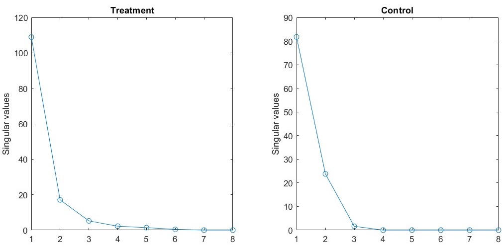
Figure 1: The singular values of the (full-sample) nuclear norm penalized estimators for the treated and control sample, i.e., $\widetilde{\mathbf{M}}^{\mathrm{full},(1)}$ and $\widetilde{\mathbf{M}}^{\mathrm{full},(0)}$, respectively, in descending order. The left corresponds to the treated sample, while the right corresponds to the control sample.

We construct the diversified weighting matrices following the observed characteristics approach explained in Section 6.1. To be specific, the columns of $\mathbf{W}_{\mathbf{F}}$ and $\mathbf{W}_{\bm{\beta}}$ consist of polynomial transformations (up to the second power) of the annual data of U.S. GDP growth rates and unemployment rates, and the state-by-state data on the average population and the count of “political swings.”

To begin with, we estimate individual state effects, i.e., the overall time average treatment effects for each state. The individual state effects and their corresponding t-statistics are presented in Figure 2. For each state, the null hypothesis is that there is no pork-barrel politics, i.e., the average treatment effect is non-positive. We reject the null hypothesis in 29 states at the 5% significance level and in 18 states at the 1% significance level. Figure 3 depicts the distribution of the states where the null hypotheses are rejected. These test results suggest that the pork-barrel politics exist in a larger number of states. We now turn to a very natural question: Why are some states enjoying the “pork,” while others are not?

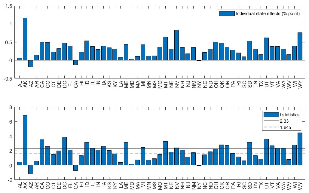
Figure 2: Individual state effects and corresponding t-statistics

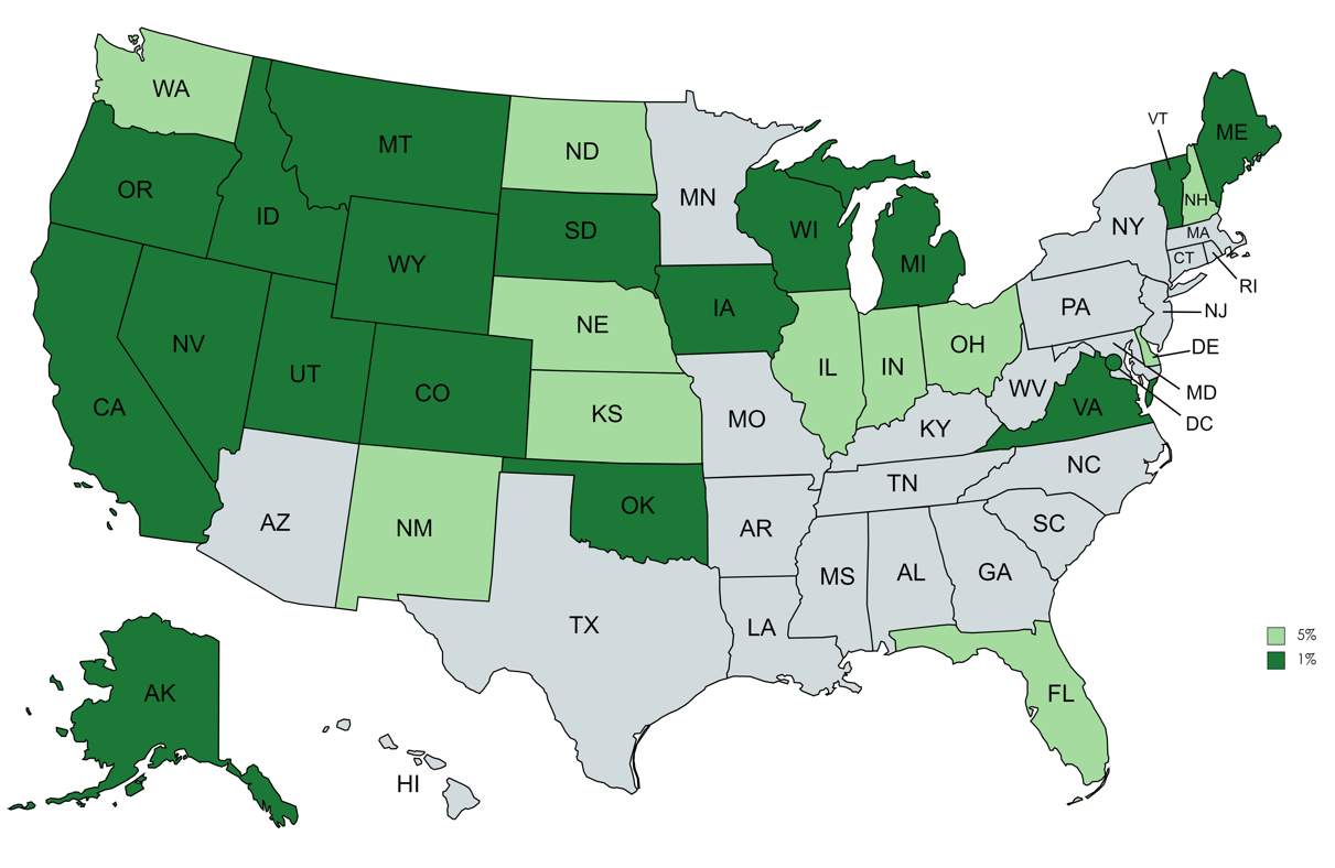
Figure 3: The states in dark green indicate the rejection of the null hypothesis at a significance level of 1%, whereas the states in light green correspond to a significance level of 5%. In the gray-colored states, the null hypotheses are not rejected. This figure is created with MapChart.

We observe that many of the states colored in dark green in Figure 3 are known as “loyal” states in that they have supported one party over decades. For example, DC has exclusively supported the Democratic Party since 1964, while AK, ID, OK, SD, UT, and WY have consistently supported the Republican Party since 1968. Inspired by this observation, we classify all 51 states based on their “loyalty” to a particular party. Specifically, we count the number of times that a state switches the party it supports, referred to as a “swing,” since the 1952 U.S. presidential election, in Table 1.

Group	# of swings	States
Swing states	8$\sim$	FL, GA, LA, OH
Weak swing states	6$\sim$7	AR, IA, KY, MS, MO, PA, TN, WV, WI
Neutral states	5	AL, CO, DE, HI, MD, MI, NV, NH, NM, NY, NC, RI
Weak loyal states	3$\sim$4	AZ, CA, CT, IL, IN, ME, MA, MN, MT, NJ, OR, SC, TX, VT, VA, WA
Loyal states	0$\sim$2	AK, DC, ID, KS, NE, ND, OK, SD, UT, WY

Table 1: The counts of swings

Based on Table 1, we estimate the overall time average treatment effects for the state groups. The first plot in Figure 4 indicates a positive relation between the loyalty and treatment effects: stronger loyalty leads to more substantial treatment effects. This “rewarding-loyalty” pattern is even clearer with t-statistics in the second plot. Also, these t-statistics show that the pork-barrel politics exist in almost all groups. Only the t-statistic of the swing states is slightly lower than 2.33, and all other t-statistics are much larger.

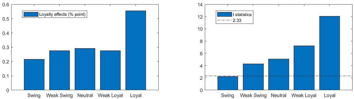
Figure 4: Loyalty effects and corresponding t-statistics

7.2 Out-of-Sample performance comparison

In this section, we conduct a comparison of out-of-sample performances of our estimator with several other estimators, using the data set described in Section 7.1.

We begin by partitioning the data $\mathbf{Y}^{(1)}$ and $\mathbf{Y}^{(0)}$ into training and testing samples. For each state $i$, we randomly sample training periods, denoted as $\mathcal{T}_{i}\subset\{1,\ldots,T\}.$ The unsampled periods are the testing periods. We note that different states have different $\mathcal{T}_{i}$, ensuring that there are some observations at each $t=1,\ldots,T$. However, we use the same $\mathcal{T}_{i}$ for both the treated and control samples. Specifically, the training sample is defined as

$$Y^{(\iota),\mathrm{train}}_{it}=\begin{cases}0&\text{if $Y^{(\iota)}_{it}$ is not observed, depending on the treatment assignment,}\\ 0&\text{if $Y^{(\iota)}_{it}$ is observed, but $t$ is not sampled, i.e., $t\notin\mathcal{T}_{i}$, and}\\ Y^{(\iota)}_{it}&\text{if $Y^{(\iota)}_{it}$ is observed, and $t\in\mathcal{T}_{i}$.}\end{cases}$$

for each $(i,t)$ and $\iota=0,1.$ Using these training samples, we estimate $\mathbf{M}^{\star,(\iota)}$ with several estimation methods including ours. For given estimators $\widehat{\mathbf{M}}^{(\iota),\mathrm{train}}$, the average treatment effect estimator for state $i$, on the testing periods, is defined as

$$\widehat{\tau}_{i}\coloneqq\frac{1}{|\mathcal{T}_{i}^{\mathrm{c}}|}\sum_{t\notin\mathcal{T}_{i}}\left(\widehat{M}^{(1),\mathrm{train}}_{it}-\widehat{M}^{(0),\mathrm{train}}_{it}\right).$$

The “quasi-true” average treatment effect estimator for each state $i$ on the testing periods is defined as $\widetilde{\tau}_{i}=A_{i}(1)-A_{i}(0)$ where, for each $\iota=0,1$,

$$A_{i}(\iota)\coloneqq\frac{1}{\sum_{t\notin\mathcal{T}_{i}}\mathbf{1}\{\text{$Y_{it}^{(\iota)}$ is observed}\}}\sum_{t\notin\mathcal{T}_{i}}Y_{it}^{(\iota)}\times\mathbf{1}\{\text{$Y_{it}^{(\iota)}$ is observed}\}.$$

We compute the out-of-sample RMSE, $\sqrt{N^{-1}\sum_{i=1}^{N}(\widehat{\tau}_{i}-\widetilde{\tau}_{i})^{2}}$, of each estimation method and report the results in Table 2. Throughout this experiment, we randomly sample $70\%$ of the total periods to define the training periods. While data-driven methods considered in Section 7.3 select $r=2$ for both $\mathbf{Y}^{(1),\mathrm{train}}$ and $\mathbf{Y}^{(0),\mathrm{train}}$, we observe that this choice does not result in optimal out-of-sample performance. Therefore, we additionally include other cases, $r=3$ to $5$, in our comparison.

For our diversified projection estimator, the rank corresponds to the number of columns in the diversified weighting matrices, denoted as $R$. As in Section 7.1, we follow the observed characteristics approach to construct the diversified weighting matrices. Although we select $R=5$ in Section 7.1, for reference, we also consider $R=2$ to $4$. Specifically, for $R=2$, we use the annual data of U.S. GDP growth rates and unemployment rates for $\mathbf{W}_{\mathbf{F}}$, and the state-by-state data on the average population and the count of “political swings” for $\mathbf{W}_{\bm{\beta}}$. For $R=3,$ we add a vector of ones (the $0$th power of an observed characteristic) to both diversified weighting matrices. For $R=4$ and $R=5$, we successively add the second power of the observed characteristics. In Table 2, “DP,” “(Hetero) LP,” “Nucl,” “TLS,” and “IPW” indicate our Diversified Projection estimator, the Low-rank Projection estimator in Chen et al., (2019) that is modified to accommodate the heterogeneous observation probabilities, the pure Nuclear norm penalized estimator, the Two-step Least Squares estimator in Choi et al., (2023), and the Inverse Probability Weighting based estimator in Xiong and Pelger, (2020), respectively.

Rank	2	3	4	5
DP	0.4921	0.4507	0.4319	0.4314
(Hetero) LP	0.4761	0.4793	0.4486	0.4505
Nucl	0.5383
TLS	0.8965	0.9056	0.8122	0.7758
IPW	1.0812	0.9635	0.8996	0.9083

Table 2: The out-of-sample RMSE

NOTE: “DP,” “(Hetero) LP,” “Nucl,” “TLS,” and “IPW” represent our Diversified Projection estimator, the modified Low-rank Projection estimator accounting for observation heterogeneity, the pure Nuclear norm penalized estimator, the Two-step Least Squares estimator, and the Inverse Probability Weighting based estimator, respectively.

We highlight two important observations from this real-data-based experiment. First, our estimator outperforms other estimators. When the rank of $\mathbf{W}_{\bm{\beta}}$ and $\mathbf{W}_{\mathbf{F}}$ is sufficiently high (recall that we chose $R=5$ in Section 7.1), the RMSE of our estimator is smaller than any other estimators with any rank specification. Second, as we progressively increase the value of $R$, the RMSE of our DP estimator decreases. This pattern suggests that we are including the relevant linear spaces more and more by adding more columns (information) to the diversified weighting matrices. This can serve as an additional rationale for setting sufficiently high $R$ in practice.

7.3 The rank estimation is not ideal

We use two data-driven rank estimations, one is based on the eigenvalue-ratio as in (see Ahn and Horenstein,, 2013) and the other is from Chernozhukov et al., (2021) and Choi et al., (2023). We apply these methods to four samples: the full samples $\mathbf{Y}^{(1)}$ and $\mathbf{Y}^{(0)}$, and the training samples $\mathbf{Y}^{(1),\mathrm{train}}$ and $\mathbf{Y}^{(0),\mathrm{train}}$ that are defined in Section 7.2. The estimated rank always turns out to be $2$. However, as highlighted in Section 7.2, this choice does not lead to optimal our-of-sample performance, for all the low-rank completion methods in Table 2. The (Hetero) LP estimator and the IPW estimator perform the best at rank 4, while our DP estimator and the TLS estimator exhibit the best performance at rank 5.

These observations suggest that there is a potential gap between the estimated rank and the rank that yields the optimal out-of-sample performance in the finite sample, which can confuse practitioners who need to select a single (and correct) value of the rank. We highlight that this conflict does not apply to our method.

References

- Abbe et al., (2020) Abbe, E., Fan, J., Wang, K., and Zhong, Y. (2020). Entrywise eigenvector analysis of random matrices with low expected rank. Annals of statistics, 48(3):1452.
- Ahn and Horenstein, (2013) Ahn, S. C. and Horenstein, A. R. (2013). Eigenvalue ratio test for the number of factors. Econometrica, 81(3):1203–1227.
- Athey et al., (2021) Athey, S., Bayati, M., Doudchenko, N., Imbens, G., and Khosravi, K. (2021). Matrix completion methods for causal panel data models. Journal of the American Statistical Association, pages 1–15.
- Bai and Ng, (2023) Bai, J. and Ng, S. (2023). Approximate factor models with weaker loadings. Journal of Econometrics.
- Barigozzi and Cho, (2020) Barigozzi, M. and Cho, H. (2020). Consistent estimation of high-dimensional factor models when the factor number is over-estimated. Electronic Journal of Statistics, 14(2):2892 – 2921.
- Bennett et al., (2007) Bennett, J., Lanning, S., et al. (2007). The netflix prize. In Proceedings of KDD cup and workshop, volume 2007, page 35. New York.
- Berry et al., (2010) Berry, C. R., Burden, B. C., and Howell, W. G. (2010). The president and the distribution of federal spending. American Political Science Review, 104(4):783–799.
- Bickel and Levina, (2008) Bickel, P. J. and Levina, E. (2008). Covariance regularization by thresholding. The Annals of Statistics, pages 2577–2604.
- Bien and Tibshirani, (2011) Bien, J. and Tibshirani, R. J. (2011). Sparse estimation of a covariance matrix. Biometrika, 98(4):807–820.
- Cai et al., (2021) Cai, C., Li, G., Chi, Y., Poor, H. V., and Chen, Y. (2021). Subspace estimation from unbalanced and incomplete data matrices: statistical guarantees. Annals of Statistics, 49(2):944–967.
- Cai and Liu, (2011) Cai, T. and Liu, W. (2011). Adaptive thresholding for sparse covariance matrix estimation. 106(494):672–684.
- Cai and Zhang, (2018) Cai, T. T. and Zhang, A. (2018). Rate-optimal perturbation bounds for singular subspaces with applications to high-dimensional statistics. The Annals of Statistics, 46(1):60–89.
- Candès and Plan, (2010) Candès, E. J. and Plan, Y. (2010). Matrix completion with noise. Proceedings of the IEEE, 98(6):925–936.
- Candès and Recht, (2009) Candès, E. J. and Recht, B. (2009). Exact matrix completion via convex optimization. Foundations of Computational mathematics, 9(6):717.
- Cape et al., (2019) Cape, J., Tang, M., and Priebe, C. E. (2019). The two-to-infinity norm and singular subspace geometry with applications to high-dimensional statistics. The Annals of Statistics, 47(5):2405–2439.
- (16) Chen, J., Liu, D., and Li, X. (2020a). Nonconvex rectangular matrix completion via gradient descent without regularization. IEEE Transactions on Information Theory, 66(9):5806–5841.
- (17) Chen, Y., Chi, Y., Fan, J., Ma, C., and Yan, Y. (2020b). Noisy matrix completion: Understanding statistical guarantees for convex relaxation via nonconvex optimization. SIAM journal on optimization, 30(4):3098–3121.
- Chen et al., (2019) Chen, Y., Fan, J., Ma, C., and Yan, Y. (2019). Inference and uncertainty quantification for noisy matrix completion. Proceedings of the National Academy of Sciences, 116(46):22931–22937.
- Chernozhukov et al., (2018) Chernozhukov, V., Hansen, C., Liao, Y., and Zhu, Y. (2018). Inference for heterogeneous effects using low-rank estimation of factor slopes. arXiv preprint arXiv:1812.08089.
- Chernozhukov et al., (2021) Chernozhukov, V., Hansen, C., Liao, Y., and Zhu, Y. (2021). Inference for low-rank models. arXiv preprint arXiv:2107.02602.
- Choi et al., (2023) Choi, J., Kwon, H., and Liao, Y. (2023). Inference for low-rank completion without sample splitting with application to treatment effect estimation. arXiv preprint arXiv:2307.16370.
- Connor et al., (2012) Connor, G., Hagmann, M., and Linton, O. (2012). Efficient semiparametric estimation of the fama–french model and extensions. Econometrica, 80(2):713–754.
- Fama and French, (1993) Fama, E. F. and French, K. R. (1993). Common risk factors in the returns on stocks and bonds. Journal of financial economics, 33(1):3–56.
- Fan and Liao, (2022) Fan, J. and Liao, Y. (2022). Learning latent factors from diversified projections and its applications to over-estimated and weak factors. Journal of the American Statistical Association, 117(538):909–924.
- Fan et al., (2013) Fan, J., Liao, Y., and Mincheva, M. (2013). Large covariance estimation by thresholding principal orthogonal complements. Journal of the Royal Statistical Society Series B: Statistical Methodology, 75(4):603–680.
- Fan et al., (2016) Fan, J., Liao, Y., and Wang, W. (2016). Projected principal component analysis in factor models. Annals of statistics, 44(1):219.
- Harper and Konstan, (2015) Harper, F. M. and Konstan, J. A. (2015). The movielens datasets: History and context. Acm transactions on interactive intelligent systems (tiis), 5(4):1–19.
- Hastie et al., (2015) Hastie, T., Mazumder, R., Lee, J. D., and Zadeh, R. (2015). Matrix completion and low-rank svd via fast alternating least squares. The Journal of Machine Learning Research, 16(1):3367–3402.
- Imbens and Rubin, (2015) Imbens, G. W. and Rubin, D. B. (2015). Causal inference in statistics, social, and biomedical sciences. Cambridge University Press.
- Johnstone and Lu, (2009) Johnstone, I. M. and Lu, A. Y. (2009). On consistency and sparsity for principal components analysis in high dimensions. Journal of the American Statistical Association, 104(486):682–693.
- Keshavan et al., (2010) Keshavan, R. H., Montanari, A., and Oh, S. (2010). Matrix completion from a few entries. IEEE transactions on information theory, 56(6):2980–2998.
- Klopp, (2014) Klopp, O. (2014). Noisy low-rank matrix completion with general sampling distribution. Bernoulli, 20(1):282–303.
- Koltchinskii et al., (2020) Koltchinskii, V., LÖFFLER, M., and NICKL, R. (2020). Efficient estimation of linear functionals of principal components. The Annals of Statistics, 48(1):464–490.
- Koltchinskii et al., (2011) Koltchinskii, V., Lounici, K., Tsybakov, A. B., et al. (2011). Nuclear-norm penalization and optimal rates for noisy low-rank matrix completion. The Annals of Statistics, 39(5):2302–2329.
- Lam and Fan, (2009) Lam, C. and Fan, J. (2009). Sparsistency and rates of convergence in large covariance matrix estimation. 37:42–54.
- Larcinese et al., (2006) Larcinese, V., Rizzo, L., and Testa, C. (2006). Allocating the us federal budget to the states: The impact of the president. The Journal of Politics, 68(2):447–456.
- Ledoit and Wolf, (2012) Ledoit, O. and Wolf, M. (2012). Nonlinear shrinkage estimation of large-dimensional covariance matrices. The Annals of Statistics, 40(2):1024–1060.
- Lounici, (2014) Lounici, K. (2014). High-dimensional covariance matrix estimation with missing observations. Bernoulli, pages 1029–1058.
- Ma and Chen, (2019) Ma, W. and Chen, G. H. (2019). Missing not at random in matrix completion: The effectiveness of estimating missingness probabilities under a low nuclear norm assumption. Advances in Neural Information Processing Systems, 32.
- Negahban and Wainwright, (2011) Negahban, S. and Wainwright, M. J. (2011). Estimation of (near) low-rank matrices with noise and high-dimensional scaling. The Annals of Statistics, 39(2):1069 – 1097.
- Negahban and Wainwright, (2012) Negahban, S. and Wainwright, M. J. (2012). Restricted strong convexity and weighted matrix completion: Optimal bounds with noise. The Journal of Machine Learning Research, 13(1):1665–1697.
- Onatski, (2012) Onatski, A. (2012). Asymptotics of the principal components estimator of large factor models with weakly influential factors. Journal of Econometrics, 168(2):244–258.
- Rubin, (1974) Rubin, D. B. (1974). Estimating causal effects of treatments in randomized and nonrandomized studies. Journal of educational Psychology, 66(5):688.
- Xia and Yuan, (2021) Xia, D. and Yuan, M. (2021). Statistical inferences of linear forms for noisy matrix completion. Journal of the Royal Statistical Society: Series B (Statistical Methodology), 83(1):58–77.
- Xia et al., (2022) Xia, D., Zhang, A. R., and Zhou, Y. (2022). Inference for low-rank tensors—no need to debias. The Annals of Statistics, 50(2):1220–1245.
- Xiong and Pelger, (2020) Xiong, R. and Pelger, M. (2020). Large dimensional latent factor modeling with missing observations and applications to causal inference. arxiv eprint. arXiv preprint arXiv:1910.08273.
- Zheng and Lafferty, (2016) Zheng, Q. and Lafferty, J. (2016). Convergence analysis for rectangular matrix completion using burer-monteiro factorization and gradient descent. arXiv preprint arXiv:1605.07051.
- Zhu et al., (2022) Zhu, Z., Wang, T., and Samworth, R. J. (2022). High-dimensional principal component analysis with heterogeneous missingness. Journal of the Royal Statistical Society Series B: Statistical Methodology, 84(5):2000–2031.