A Geometric Tension Dynamics Model of Epithelial Convergent Extension

Abstract

Epithelial tissue elongation by convergent extension is a key motif of animal morphogenesis. On a coarse scale, cell motion resembles laminar fluid flow; yet in contrast to a fluid, epithelial cells adhere to each other and maintain the tissue layer under actively generated internal tension. To resolve this apparent paradox, we formulate a model in which tissue flow occurs through adiabatic remodelling of the cellular force balance causing local cell rearrangement. We propose that the gradual shifting of the force balance is caused by positive feedback on myosin-generated cytoskeletal tension. Shifting force balance within a tension network causes active T1s oriented by the global anisotropy of tension. Rigidity of cells against shape changes converts the oriented internal rearrangements into net tissue deformation. Strikingly, we find that the total amount of tissue extension depends on the initial magnitude of anisotropy and on cellular packing order. T1s degrade this order so that tissue flow is self-limiting. We explain these findings by showing that coordination of T1s depends on coherence in local tension configurations, quantified by a certain order parameter in tension space. Our model reproduces the salient tissue- and cell-scale features of germ band elongation during Drosophila gastrulation, in particular the slowdown of tissue flow after approximately twofold extension concomitant with a loss of order in tension configurations. This suggests local cell geometry contains morphogenetic information and yields predictions testable in future experiments. Furthermore, our focus on defining biologically controlled active tension dynamics on the manifold of force-balanced states may provide a general approach to the description of morphogenetic flow.

Shape changes of epithelia during animal development involve major cell rearrangements, often manifested as a “convergent extension” of cell sheets. On the the coarse scale, convergent extension looks much like the laminar shear flow of an incompressible fluid in the vicinity of a hyperbolic fixed point (see Fig. 1A). Indeed, previous work has combined hydrodynamic equations for the mesoscale cell velocity field with active stress fields to model morphogenetic tissue flow [1, 2, 3, 4]. Yet in contrast to a fluid, epithelia are under internally generated tension – revealed by laser ablation [5] – and, like solids, maintain their shape against external forces. Tissue flow is achieved through local cell intercalation (T1 neighbor exchange processes, see Fig. 1B) driven by the concerted mechanical activity of individual cells. Cells generate forces via actomyosin contractility in the cortical cytoskeleton at the adherens junctions between cells (Fig. 1C). Moreover, the adherens junctions can remodel through the turnover of its constituent molecules. Taken together, this implies that interfaces in the cell array can change their length and tension independently. This behavior is fundamentally different from (Hookean) springs, where tension and length are related by a constitutive relationship. Instead, one can imagine cellular interfaces as “microscopic muscles” which are controlled by the recruitment and release of myosin motors.

Vertex models generally describe epithelial tissue as a polygonal tiling of cells where the vertex positions are the dynamical variables [6, 7]. The forces that drive the vertex motion are commonly derived from passive area and perimeter elasticity supplemented with additional active tensions [8, 9, 10]. However, the muscle metaphor for cellular interfaces suggests that they form a mechanical network dominated by active tension (Fig. 1D). This network rapidly equilibrates to a force balanced state [11, 5, 12], stabilized by mechanical feedback loops [13, 14]. In such an active tension network, passive elasticity plays a subdominant role. The need for stabilizing feedback loops arises because active tensions are untethered from interface lengths. Indeed, on an abstract level, these feedback loops are not unlike the regulatory mechanisms that control and stabilize skeletal musculature [15].

Here, we propose that tissue flow can be understood in the terms of an adiabatic remodeling of internal active force balance. Force balance in the cortical tension network defines a manifold of cellular tiling geometries on which tissue deformation unfolds. We propose that dynamics in the force-balance manifold driven by positive feedback on the cortical tensions. This view is supported by analysis of high quality live imaging data [16] from Drosophila gastrulation presented in the companion paper [17]. Specifically, tension inference has provided evidence for the role of positive tension feedback during active T1 events. Numerical simulations of cell quartets show that such a feedback mechanism is sufficient to drive the T1 process. However, the question of coordination of T1s across the tissue – required to drive coherent tissue flow – has remained unanswered. To address this question, we develop a model of tissue mechanics in the tension-dominated regime and demonstrate via numerical simulations how positive feedback drives convergent extension. We show that order of the cell packing is necessary for coordinating T1 processes, and hence efficient convergent extension. T1s destroy this order such that the extent of tissue flow is self limiting. Thereby, our model reproduces the experimentally observed elongation of the germband where the arrest of flow is concomitant with a transition from an ordered to a disordered cell packing [17].

Methods

A minimal model based on force balance and cell geometry.

Our model is based on the assumption that on the timescales relevant to morphogenetic dynamics, the dominant active forces in the epithelium (generated by contractile myosin-2 motors in the adherens junctions, see Fig. 1C) are approximately balanced. In particular, we assume that adhesion forces between the epithelial layer and its substrate (the fluid yolk in the case of the Drosophila embryo) caused by the relatively slow morphogenetic motion, are negligible. Hence, all forces must be balanced within the transcellular network of cellular junctions. We model the tissue in the general framework of vertex models (see e.g. [7]) as a polygonal tiling of the plane with tri-cellular vertices $\mathbf{r}_{ijk}$, where each polygon represents a cell $i$ (see Fig 1D). Since we focus on a setting where active cortical tensions dominate over passive elasticity, we write the elastic energy differential of this network as

$$\delta\mathcal{E}(\{\mathbf{r}_{ijk}\}|\{T_{ij}\})=\sum_{ij}T_{ij}d\ell_{ij}-p\sum_{i}dA_{i}+\varepsilon\sum_{i}dE_{\mathcal{C}}(S_{i}),$$ (1)

where $\varepsilon$ is a small parameter that separates the scale of active and passive mechanical contributions. $E_{\mathcal{C}}(S_{i})$ accounts for the passive elasticity of the cells and will be specified below; $\ell_{ij}=||\mathbf{r}_{ij}||$ is the length of the interface between adjacent cells $i$ and $j$ and $T_{ij}$ is the cortical tension at that interface. Importantly, in contrast with the standard vertex model, where edge tension is defined by a constitutive relation corresponding to a passive Hookean perimeter spring, we take cortical tensions to be controlled independently of the interface lengths. The tension dynamics is described in the next section. The second term in Eq. (1) accounts for the effective in-plane pressure $p$ of the cells that, by maintaining the total surface area (sum over individual cell areas $A_{i}$), ensures that the tissue as a whole does not collapse. We assume that pressure differences between cells are small and therefore absorb them into $E_{\mathcal{C}}(S_{i})$.

We further assume a separation of scales between the timescale on which the elastic energy relaxes and the timescale on which the tissue deforms macroscopically. In other words, we assume relaxational dynamics $\gamma\partial_{t}\mathbf{r}_{ijk}=-\frac{\partial\mathcal{E}}{\partial\mathbf{r}_{ijk}}$, with a relaxation rate $\gamma^{-1}$ much faster than all other timescales in the system. (Rather than frictional dissipation, one could use viscous dissipation here). Quasi-static force balance then implies

$$\frac{\partial\mathcal{E}}{\partial\mathbf{r}_{ijk}}=0.$$ (2)

Solving this equation to zeroth order in $\varepsilon$ yields a force-balance constraints at each vertex. These constraints imply that the tension vectors $\mathbf{T}_{ij}=T_{ij}\mathbf{e}_{ij}$ at each vertex sum to zero and hence form a triangle. Since neighboring vertices share the interface that connects them, the corresponding tension triangles share an edge. Therefore, all tension triangles have to fit together to tile the plane: they form a triangulation that is dual to the the cell tiling [13, 18, 19]. In force balance, angles at real-space vertices are complementary to tension triangle angles. Therefore, given a tension triangulation $\{T_{ij}\}$, minimization of the elastic energy $\mathcal{E}$ at zeroth order in $\varepsilon$ fixes the angles at all vertices in the cellular tessellation. Importantly, fixing the angles at vertices does not fully determine the cell tessellation, i.e. the $\mathbf{r}_{ijk}$ remain underdetermined, as this leaves the freedom to change the interface lengths $\ell_{ij}$ while preserving all angles. The resulting isogonal modes thus account for interface length changes under constant tension [13], which is possible thanks to the turnover of cytoskeletal elements. The isogonal modes can dilate and shear cells (Fig 1F) and thus contribute elastic energy of order $\epsilon$ via the cell shape energy $E_{\mathcal{C}}(S_{i})$. By our hypothesis, this contribution is substantially smaller than the active cortical tensions such that isogonal deformations act as “soft modes” with relatively large deformations produced by small forces. Cells resist shape distortions due to rigid cell-internal structures such as microtubules, the nucleus [20], and intermediate filaments [21]. To account for this passive cell elasticity, we propose an energy

$$E_{\mathcal{C}}(S)=\lambda[\mathrm{Tr}(S-S_{0})]^{2}+\mu\mathrm{Tr}[(S-S_{0})^{2}],$$ (3)

in terms of the cell shape tensor

$$S_{i}=\sum_{k\in\mathcal{N}_{i}}\frac{\mathbf{r}_{ik}\otimes\mathbf{r}_{ik}}{\ell_{ik}},$$ (4)

where $\mathcal{N}_{i}$ is the set neighbors of cell $i$. The shape tensor is defined such that it is invariant under subdivision of interfaces. The reference tensor $S_{0}$ controls the target cell shape and is given by $S_{0}=3\ell_{0}\;\mathbb{I}$ for an isotropic hexagonal cell with side length $\ell_{0}$.

Minimization of $\sum_{i}E_{\mathcal{C}}(S_{i})$ while keeping all angles fixed determines the isogonal degrees of freedom and therefore determines the quasi-stationary cell tessellation for a given tension triangulation (Fig 1F). A simple counting of degrees of freedom shows that there is one isogonal degree of freedom per cell [13]. Therefore, the isogonal modes can be parametrized by an “isogonal function” that takes a scalar value in each cell. The isogonal displacement of a vertex is defined in terms of the values of this isogonal function in the three adjacent cells (see Eq. (17)).

External forces will deform the cell tessellation by acting on the isogonal modes. We can therefore relate cell rigidity and tissue rigidity by analyzing the energy spectrum of isogonal modes for a given tension triangulation (see SI Sec. III.2). The two isogonal modes with the lowest energy correspond to uniform pure shear (see Fig. S10A). From these eigenmodes, we find a linear relationship between the cell and tissue shear moduli (see Fig. S10B).

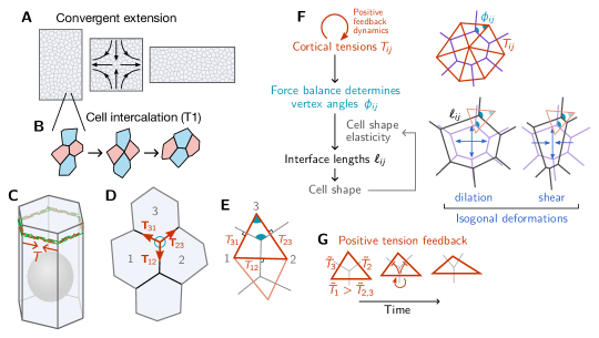
Figure 1: Tissue mechanics dominated by cortical tension. A Convergent extension of epithelial tissue by cell intercalations (T1 processes, B). C A single cell from a columnar epithelium with the actomyosin cortex at the adherens junction belt generating tension $T$ along cell-cell interfaces. Gray sphere represents the nucleus. D In force balance, the tensile forces $\mathbf{T}_{ij}$ at each vertex must sum to zero, thus linking the tensions to the angles at which the interfaces meet. E Force balance implies that the tensile force vectors at each vertex form a triangle. Triangles at neighboring vertices share an edge and thus form a triangulation that tiles the plane. The angles in the tension triangulation are complimentary to the angles in the tissue. F Outline of our tissue model with mechanics dominated by actively regulated cortical tensions. Tension dynamics in adiabatic force balance are formulated as a geometric model of the tension triangulation which determines the angles at vertices. The remaining isogonal (angle-preserving) degrees of freedom are governed by cell-shape elastic energy, which accounts for (passive) non-cortical elasticity and penalizes dilation and shearing. G We propose tension dynamics governed by positive tension feedback where the longest edge in a tension triangle grows at the expense of its neighbors.

Positive feedback and adiabatic dynamics

On the timescale of morphogenetic flow, tensions change due to the recruitment and release of molecular motors, driving the remodeling of the force balance geometry encoded in the tension triangulation. To complete the model, we need to specify the dynamics that governs the tensions on this slow timescale. Based on previous experiments [22] and models [23, 10], we propose a positive feedback mechanism where tension leads to further recruitment of myosin and thus further increase in tension. This self-amplifying accumulation of myosin on individual interfaces is limited by the competition for a limited pool of myosin within each cell. To mimic this local competition for myosin in a computationally simple way, we constrain tension dynamics to conserve the perimeter of each tension triangle, i.e. the sum of tensions at each vertex $(ijk)$. For an individual triangle with tensions $\tilde{T}_{1},\tilde{T}_{2},\tilde{T}_{3}$, we consider the dynamics

$$\tau_{\mathrm{T}}\partial_{t}\tilde{T}_{\alpha}=\tilde{T}_{\alpha}^{n}-\frac{1}{3}\sum_{\beta=1}^{3}\tilde{T}_{\beta}^{n},\quad\text{with}\quad\alpha=\{1,2,3\}$$ (5)

Note that this feedback mechanism has a “winner-takes-all” character, where the longest edge in the tension triangle always outgrows the other two, as illustrated in Fig 1G. This is only one of of many possible models: below we will shall also investigate a positive tension feedback that saturates and leads to qualitatively different tissue dynamics.

Force balance requires that that all tension triangles fit together to form a flat triangulation [13]. The triangulation is parameterized by a set of 2D tension vertex positions $\mathbf{t}_{i}$, so that the tension on edge $(ij)$ is given by $T_{ij}=||\mathbf{t}_{i}-\mathbf{t}_{j}||$. In each iteration of the simulation, the tension vertices $\mathbf{t}_{i}$ are determined by fitting the balanced tensions $T_{ij}$ to the intrinsic tensions $\tilde{T}_{ij}$ using a least squares method. In addition, the intrinsic tensions $\tilde{T}_{ij}$ relax to the balanced tensions $T_{ij}$ with a rate $\tau_{\mathrm{balance}}^{-1}$ (see SI Sec. IV for details). This “balancing” of the tension triangulation effectively accounts for small pressure differentials and additional feedback mechanisms (such as strain rate feedback [13]) which maintain the tension network in a state compatible with force balance. The rate at which these mechanisms act is controlled by the timescale $\tau_{\mathrm{balance}}$ which we assume to be much smaller than the timescale $\tau_{\mathrm{T}}$ on which tension evolve due to positive feedback.

The above dynamics is autonomous in tension space until an edge in the cell tessellation reaches length zero. At this point, a cell neighbor exchange (T1 transition) occurs, corresponding to an edge flip in the tension triangulation. After this topological modification, the tension dynamics continues autonomously again until the next T1 event. To determine the active tension (i.e. myosin level) on the new interface formed during the cell neighbor exchange, we assume continuity of myosin concentration at vertices as described in the companion paper [17] and in SI Sec. IV. The active tension is not sufficient to balance the total tension on the new interface, such that passive elements of the cortex (e.g. crosslinkers) are transiently loaded. The resulting passive tension relaxes due to remodeling with timescale $\tau_{\mathrm{p}}$ (see SI Sec. IV for details). This relaxation causes the elongation of the new interface as it transiently counteracts positive tension feedback and thereby prevents the new interface from immediately re-collapsing after a T1.

This concludes the description of the computational model. A brief overview over the parameters an their effects, several of which will be discussed in detail below, is given in SI Table 1 and Fig. S7.

Results

Cell packing order facilitates self-organized convergent–extension flow

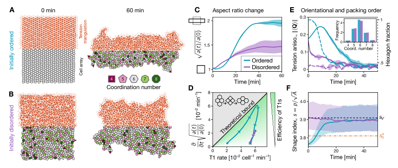
Figure 2: Extent of tissue flow depends on initial cell-scale order and tension anisotropy. A, B Simulation snapshots of tissue patches with free boundaries starting from an (irregular) hexagonal cell array (A) and a disordered cell array (B) generated from a random Voronoi tessellation. The net deformation is significantly smaller in the latter case. In both cases the final configuration is disordered. Each snapshot shows the top half of the tension triangulation and the bottom half of the corresponding cell array. Note the the initial initial tension triangulation is stretched along the $x$ direction and compressed along the $y$ direction as a result of the prescribed initial tension anisotropy. C Convergent extension is slower and ceases at a smaller net deformation for a disordered initial condition (cyan line) compared to the initially ordered case (purple line). Shaded bands indicate standard deviation over $N=3$ simulation runs with $N_{\mathrm{cells}}\approx 10^{3}$ cells each. D Plotting the rate of tissue convergent extension against the T1 rate provides a measure for the efficiency of T1 transitions. For the initially ordered tissue, the efficiency of T1s is starts out near the theoretical optimum but drops to zero as the tissue becomes disordered. For the disordered initial condition, T1s are inefficient from the beginning. The theoretical bound (for cells retaining isotropic shape) is a factor of $\sqrt{3}$ elongation for 2 T1s per cell as illustrated in the inset cartoon. E Decreasing hexagon fraction (solid lines) and global tension anisotropy (dashed lines) indicate the decay of order in the cell arrays. Notably, in the initially ordered cell array, tension anisotropy transiently increases due to positive tension feedback (solid purple line). At late times both simulations converge to zero global tension anisotropy and identical coordination number statistics (inset). F As order is lost, the cell-shape index $s$ converges to that of a random Voronoi tessellation $s_{\mathrm{V}}$ (dashed black line). Note that the critical shape index for the rigidity transition in the “classical” vertex model [24], $s_{0}^{*}\approx 3.81$ (dot-dashed orange line), does not feature in our results. Lines show the median, shaded bands indicates quartiles.

In the companion paper [17], we have shown that positive tension feedback can drive an active T1 transition in a cell quartet where the inner interface is initially under slightly higher tension than its neighbors. The simulations in Ref. [17] were performed in a quartet of identical cells, representing a perfectly regular lattice of cells. However, any real tissue will exhibit some degree of irregularity. Investigating the effect of this disorder is key to understand convergent extension on the tissue scale. To this end, we perform simulations of irregular cell arrays. All parameters are set to the same values as in the companion paper, where the time scale $\tau_{T}$ was calibrated to fit the tension and interface length dynamics of active T1s during Drosophila gastrulation. We start with simulations of a freely suspended patch of tissue to investigate the role of initial tension anisotropy and order in the cell packing. Further below, we will present simulations that combine active with passive tissue regions, mimicking the Drosophila germ band and the adjacent amnioserosa tissue.

Starting with a slightly perturbed hexagonal cell packing, the tissue patch undergoes convergent extension elongating the tissue perpendicular to the initial orientation of global tension anisotropy (Fig. 2A). The tissue flow is driven by self-organized cell rearrangements (active T1 transitions) whose rate rapidly increases, reaching a maximum, and then decreases to a lower, but non-zero, value (Fig. 2D). Large-scale tissue deformation stalls after approximately 2-fold convergent extension (as measured by the square root of the aspect ratio $a=\mathrm{width}/\mathrm{height}$, Fig. 2C) while cells continue rearranging. This suggests that T1s at this stage are no longer coherently oriented and therefore do not contribute to net tissue deformation. Indeed, the efficiency of T1s at driving convergent extension drops after the T1 rate has peaked (Fig. 2D).

As cells rearrange, the tissue becomes increasingly disordered, as indicated by the loss of global tension anisotropy and the decreasing fraction of cells with six neighbors, $p_{6}$ (Fig. 2E). We define the tension anisotropy tensor $Q=\tfrac{2}{3}\sum_{\alpha=1}^{3}\mathbf{T}_{\alpha}\otimes\mathbf{T}_{\alpha}$ directly from the tension geometry ($Q$ can be thought of as the metric tensor of the of the tension triangulation). Averaging the deviatoric part $\tilde{Q}=Q-\frac{1}{2}\mathrm{Tr}\,Q$ over the cell array, we obtain a measure of global tension anisotropy $||\langle\sqrt{2}\tilde{Q}\rangle||\in[0,1]$.

To test the role of initial order in the cell packing, we initialize the simulation from a random Voronoi tessellation, which results in slower convergent–extension flow and arrest of flow at a smaller amount of total tissue-scale deformation (Fig. 2B, C and Movie 2). Notably, tension anisotropy rapidly vanishes without the transient increase observed in the simulation starting with a more ordered cell packing (Fig. 2E). While the early dynamics depends sensitively on the initial condition, we find rapid convergence toward a common disordered steady state.

A common measure for the degree of order in a polygonal tiling is the cell shape index ($s=P/\sqrt{A}$, with cell perimeter $P$ and area $A$), shown in Fig. 2F. This shape index is high when cell shapes are elongated or irregular and approaches the minimal value $s\approx 3.72$ for a regular hexagon. The shape index has a particular relevance in vertex models employing an area-perimeter based elastic energy [7, 24]. In these models, the target shape index is a control parameter that drives a solid to fluid transition [24]: a high target shape index ($s_{0}>s_{0}^{*}\approx 3.81$) is associated with tissue fluidity since it allows for cell rearrangements, while a low cell target shape index gives rise to a solid state. In both cases, the observed shape index is controlled by the target shape index. In contrast, in our simulations with actively driven T1s, disorder, and thus a high observed shape index, is the consequence of cell rearrangements, rather than their cause. Notably, we find more tissue flow when the observed shape index is initially low (Fig. 2F). The question of the solid vs fluid character of tissue will be addressed in more detail in the last part of the results section and in the discussion.

To systematically investigate the role of tension anisotropy and cell packing order on self-organized convergent extension, we generate tension triangulations from random hard disk packings at different packing fractions $\rho$ [25, 26]. Specifically, we sample the positions of the tension vertices $\mathbf{t}_{i}$ from a hard disk process, and then construct the corresponding Delaunay triangulation. At low packing fraction, the hard disc process generates highly irregular triangulations with broadly distributed coordination numbers (see Fig. 2B). In contrast, at sufficiently high packing fraction $\rho\gtrsim 0.72$, the disks adopt a crystalline hexagonal packing such that $p_{6}\approx 1$. The plot at the bottom of Figure 3A shows how the degree of order continuously varies with $\rho$ between these two extremes. To tune the initial tension anisotropy, the triangulation is sheared with magnitude $s$ (displacing vertices by $\mathbf{t}_{i}\mapsto\mathrm{diag}(\sqrt{1+s},1/\sqrt{1+s})\,\mathbf{t}_{i}$).

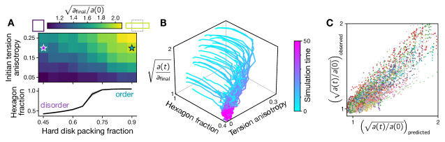
Figure 3: Hexagon fraction and tension anisotropy predict tissue flow. A The total amount of convergent-extension (overall tissue aspect ratio change $a_{\mathrm{final}}/a(0)$) increases as a function of cell packing order (controlled by hard disk packing fraction $\rho$ used to generate the Voronoi seed points) and initial tension anisotropy (controlled by a strain $s$ applied to the tension triangulation). The hard disk packing fraction $\rho$ controls the fraction of hexagonal cells (bottom). The purple and green stars indicate the initial condition parameters used for Fig. 2A and B. B Hexagon fraction, $p_{6}$, and tension anisotropy $||\langle\sqrt{2}\tilde{Q}\rangle||$ decrease as cells rearrange and eventually converge to a fixed point where anisotropy vanishes and the hexagon fraction matches a random Voronoi tessellation ($\sim 0.4$). At this point, convergent-extension flow, as measured by the remaining change in tissue aspect ratio $a_{\mathrm{final}}/a(t)$, stalls (cf. Fig. 2C, E). The trajectories approximately collapse onto a plane, suggesting that a linear relationship can predict the convergent-extension in terms of $p_{6}$ and $||\langle\sqrt{2}\tilde{Q}\rangle||$; see Eq. (6). C Correlation between predicted and observed change in aspect ratio. Data points are from simulations with initial conditions, spanning the entire parameter diagram in (A), showing that the prediction works across many different initial conditions. Points with the same color indicate different time point from the same simulation.

The heatmap in Fig. 3A (top) shows the dependence of convergent extension on the initial configuration controlled by $\rho$ and $s$. The the total extent of convergent extension, quantified by the net change in aspect ratio $\sqrt{a_{\mathrm{final}}/a_{\mathrm{initial}}}$ increases continuously with both the initial order and the magnitude of tension anisotropy. As we have seen above, both these quantities decrease as cells rearrange (cf. Fig. 2E). In fact, when plotting the remaining extent of convergent extension $\sqrt{a_{\mathrm{final}}/a(t)}$ against $p_{6}(t)$ and $||\langle\sqrt{2}\tilde{Q}(t)\rangle||$, we find trajectories that approximately lie in a common plane and converge to a fixed point at vanishing anisotropy $||\langle\sqrt{2}\tilde{Q}\rangle||\approx 0$ and $p_{6}\approx 0.4$ (Fig. 3B). Based on these results, we hypothesize an empirical law for feedback-driven convergent extension, based on the instantaneous hexagon fraction and tension anisotropy:

$$\sqrt{\frac{a_{\mathrm{final}}}{a(t)}}\approx c_{Q}||\langle\sqrt{2}\tilde{Q}(t)\rangle||+c_{6}p_{6}(t)$$ (6)

With the coefficients determined by a linear fit, Eq. (6) predicts the remaining extent of convergent extension with less than 10% mean absolute error (Fig. 3C). The empirical relation Eq. (6) is specific to the particular choice of microscopic tension dynamics employed in the simulations. A more systematic investigation of such empirical laws linking microscopic ($p_{6},||\langle\sqrt{2}\tilde{Q}(t)\rangle||$) and macroscopic ($a(t)$) quantities goes beyond the scope of this work but is an exciting avenue for future research.

Above, we have focused on degree of order in the topology (i.e. coordination numbers) of the triangulation, quantified by $p_{6}$ and controlled by the packing fraction of the hard disk seeding process. A more mild form disorder is due to random displacements of the triangulation vertices while keeping the topology fixed. The topological constraint dictates that the vertex displacements must be relatively small, and we find that they have a correspondingly small effect on the convergence-extension flow (see Fig. S7).

The model introduced above implements a specific form of positive tension feedback, Eq. (5), in such a way that total tension is conserved locally. We find qualitatively similar results for tension dynamics with different local conservation laws. Notably, positive feedback conserving areas of tension triangle instead of their perimeters produces slightly more convergent extension and exhibits an even stronger dependence of tissue flow on the initial degree of order (see SI Sec. II.1). How tissue dynamics depends on the parameters $\tau_{\mathrm{balance}},\mu,\lambda,n$ is summarized in SI Table 1 and Fig. S7. We will return to the effect of specific parameters throughout the following sections.

Taken together, our model reproduces several salient features of germ-band extension in the Drosophila embryo. We find that convergent extension driven by positive tension feedback is self-limiting and naturally explains the transition from the fast to the slow phase of germ-band extension [17]. It also reproduces that the slowdown of convergent extension is concomitant with an increase in cell-scale disorder, approaching a maximally disordered state [27, 17]. Our model suggests that the transient fast phase of flow is facilitated by an initial hexagonal packing of the cells. In the Drosophila embryo, this packing results from physical interactions of the spindle apparatuses during the syncytial cell division cycles that precede cellularization [28, 29]. Quantification of hexagonal order in the experimental data are show in Fig. S1. We predict that disrupting the initial cell packing will cause GBE to become slower. The experimental data analysis in Ref. [17] also demonstrates the presence of large-scale tension anisotropy of the order of $20\%$ before the onset of convergent extension, which in the model is required to orient tissue flow. More broadly, our results suggest that convergence extension via positive tension feedback may generally be self-limiting, as also observed in a recent model [10].

Order in local tension configurations

So far, we have focused on the role of initial topological order in the cell packing. In the Drosophila germ band, we additionally observed a more subtle form of geometric order—a particular pattern of alternating high and low tensions [17]—that precedes the onset of cell rearrangements. This cell-scale tension pattern is not apparent initially but arises dynamically in conjunction with an increase in overall tension anisotropy which suggests that this tension pattern arises from the positive tension feedback. As we show in the following, systematically quantifying the local configurations of cortical tensions provides a method to constrain physical models of cell rearrangements in epithelia.

Local tension configuration parameter.

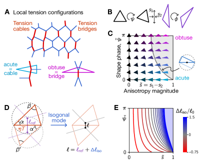
Figure 4: Triangle shape space characterises the local tension motifs that underlie cell rearrangements. A We distinguish two tension patterns, “cables” and “bridges”, by their elementary motifs of tension configuration at individual vertices. These configurations can be quantified in terms of the tension triangle shapes which we use to define a local tension configuration (LTC) parameter. B Shape decomposition of a triangle into a sequence of three transformations acting on an equilateral reference triangle. The angle $\psi$ and the shear factors $s_{1,2}$ determine the intrinsic shape of the triangle while the angle $\phi$ determines its orientation in space. C The intrinsic shape of triangles can be quantified by a complex order parameter $\tilde{s}\,e^{i\tilde{\psi}}$, where the LTC magnitude $\tilde{s}$ is proportional to the triangle’s anisotropy and the LTC phase $\tilde{\psi}$ distinguishes obtuse and acute triangles. The gray line indicates the Delaunay condition for a pair of identical triangles. Along this line, the circumcenters of the two triangles coincide, corresponding to a fourfold vertex in the Voronoi tessellation. This line therefore defines a threshold for T1 events in the case of vanishing isogonal strain. D Circumcircle construction of the Voronoi edge length (purple) from a pair of adjacent (tension) triangles (red). Circumcircles are indicated by gray dashed lines. The actual physical length $\ell$ is the sum of the Voronoi reference length $\ell_{\mathrm{ref}}$, and a contribution from isogonal strain $\Delta\ell_{\mathrm{iso}}$. In the illustration, $\Delta\ell_{\mathrm{iso}}/\ell_{0}$ is negative. E T1 threshold as a function of the isogonal strain $\Delta\ell_{\mathrm{iso}}/\ell_{0}$. Positive isogonal strain shifts the threshold to higher tension anisotropy.

The elementary motifs of a cell-scale tension pattern are the tension configurations at individual vertices. In force balance, the tension vectors at each vertex form a triangle. This allows one to characterize the tension configuration based on the shape of the tension triangle: acute triangles correspond to tension cables (adjacent high tension interfaces) while obtuse triangles correspond to an isolated high tension interface which we refer to as a tension “bridge”. The latter configuration is the elementary motif of an alternating pattern of high and low tensions as illustrated in Fig. 4A.

To quantify the relative abundance of these motifs, we define a local tension configuration (LTC) parameter that measures how anisotropic and how acute vs obtuse the tension triangle is. Given the three tension vectors $\mathbf{T}_{\alpha},\alpha=1,2,3$ that form the tension triangle, we first use the force-balance condition $\sum_{\alpha}\mathbf{T}_{\alpha}=0$ to define the reduced barycentric vectors, combined into a 2$\times$2 matrix

$$\mathfrak{T}=\begin{pmatrix}\bm{\tau}_{1}\\ \bm{\tau}_{2}\end{pmatrix}=\frac{1}{\sqrt{2}\,\mathcal{N}}\begin{pmatrix}T_{1}^{x}-T_{2}^{x}&T_{1}^{y}-T_{2}^{y}\\ \sqrt{3}\,T_{3}^{x}&\sqrt{3}\,T_{3}^{y}\end{pmatrix}.$$ (7)

where the normalization factor $\mathcal{N}$ ensures $||\mathfrak{T}||^{2}=\mathrm{Tr}[\mathfrak{T}\mathfrak{T}^{T}]=1$. This normalization fixes the arbitrary overall tension scale. Note that $\mathfrak{T}$ is not a symmetric matrix and that its indices belong to different spaces: the first labels the barycentric component and the second the Cartesian coordinate. We now carry out a singular value decomposition (SVD):

$$\mathfrak{T}=R(\psi)\cdot\begin{pmatrix}\sqrt{s_{1}}&0\\ 0&\sqrt{s_{2}}\end{pmatrix}\cdot R^{T}(\phi),$$ (8)

where $R(\alpha)$ is the rotation matrix with angle $\alpha$, singular values $s_{1}>s_{2}>0$ by convention, and $s_{1}+s_{2}=1$ because we have normalized the tension vectors. We now introduce the complex order parameter

$$\tilde{s}\,e^{i\tilde{\psi}}:=(s_{1}-s_{2})\;e^{i|3\psi\;\text{mod}_{-\pi}\;2\pi|},$$ (9)

which provides a complete description of the triangle’s intrinsic shape. (In the exponent, $a\;\text{mod}_{x}\;b=(a-x\bmod b)+x$ is the modulo function with offset $x$). Applied to tension triangles, this defines an LTC order parameter that informs about the configuration of tensions at a vertex.

The magnitude $\tilde{s}=s_{2}-s_{1}=||\sqrt{2}\tilde{Q}||\in[0,1]$ measures the triangle’s anisotropy (note that $Q=\mathfrak{T}^{T}\mathfrak{T}$) and the reduced “LTC phase” $\tilde{\psi}$ measures the triangle’s degree of acuteness vs obtuseness. Its definition is such that the redundancy in $\psi$ due to permutations of the triangle edge labels $1,2,3$ in Eq. (7) is removed. We note that the sign of $3\psi\;\text{mod}_{-\pi}\;2\pi$ indicates the chirality of the triangle’s shape, which might be useful to detect chiral symmetry breaking on the cellular scale, e.g. in the Drosophila hindgut [31].

Geometrically, the SVD of $\mathfrak{T}$ can be understood as a sequence of transformations that map an equilateral reference triangle (with one edge parallel to the $x$-axis) to the target triangle (Fig. 4B). The reference triangle is first rotated by an angle $\psi$, then stretched along the $x$- and $y$-axis with factors $s_{1}$ and $s_{2}$, and finally rotated again by an angle $-\phi$ (the minus sign results from the convention in defining SVD). $\phi$ therefore determines the triangle’s axis of anisotropy while $\psi$ determines the orientation of the shear axis to one of the edges of the original equilateral triangle. For $\psi=0$, the shear is orthogonal to a triangle side, yielding an isoceles obtuse triangle. Increasing $\psi$ makes the resulting triangle more acute, until maximal acuteness is reached at $\psi=\pi/3$.

Generalized Delaunay condition (T1 threshold).

Before we use the LTC parameter to quantify the tension space dynamics from simulations and experiments, we define a condition in the LTC space for when a T1 transitions will hapen. This T1 threshold puts a constraint on the local tension configurations that we expect to observe. Moreover, it will allow us to quantify how tension dynamics causes active T1s by driving the local tension configurations towards the T1 threshold.

Let us for a moment neglect the isogonal modes. From the tension triangulation we construct the corresponding Voronoi tessellation whose vertices are the circumcircle centers of the triangles as illustrated in Fig. 4D. The edges of the Voronoi tessellation are orthogonal to those of the triangulation, which implies that it obeys the force balance constraints, and can be used as a reference for the family of cell arrays compatible with the tension triangulation. The length of a Voronoi edge corresponding to a pair of adjacent triangles is given by

$$\ell_{\mathrm{ref}}=\frac{\sqrt{3}\,\ell_{0}T}{2}(\cot{\beta}+\cot{\beta^{\prime}}),$$ (10)

where $T$ length of the shared triangle edge interface and $\ell_{0}$ fixes the length scale such that $\ell_{0}$ is the edge length of a regular hexagonal cell, corresponding to equilateral tension triangles with $T=1$. $\ell_{\mathrm{ref}}$ changes sign at $\beta+\beta^{\prime}=\pi$, which gives the “Delaunay condition” $\beta+\beta^{\prime}<\pi$. In the absence of isogonal strain, a cell neighbor exchange (corresponding to an edge flip in the triangulation) occurs at this threshold. In Fig. 4C, the gray line indicates this threshold for a pair of identical triangles (i.e. $\beta=\beta^{\prime}=\pi/2$). Notably, the threshold is at a much smaller anisotropy magnitude $\tilde{s}$ for tension cables (small $\tilde{\psi}$) than for bridges (large $\tilde{\psi}$), implying that tension cables are less efficient at driving intercalations than tension bridges.

In passing, we note that the Delaunay condition can be used to perform simulations of a simplified model that neglects the isogonal modes and operates entirely in tension space. Simulations of this Tension-Driven Voronoi model, run orders of magnitude faster than the full model since minimizing the passive elastic energy to determine the isogonal degrees of freedom is the computationally most expensive step (see also SI Sec. II.4). In the tension-driven Voronoi model, the physical configuration is constructed from the tension triangulation Delaunay–Voronoi duality, i.e. $\ell=\ell_{\mathrm{ref}}$. Neighbor exchanges are then governed by the standard Delaunay condition similarly to the self-propelled Voronoi model which has been introduced as a simplified version of the classical vertex model [32, 33]. The fundamental difference between the tension-driven Voroni model and the self-propelled Voronoi model is that the dynamics is driven by cortical tensions in the former while driven by self-propulsion forces acting on a substrate in the latter.

How does the Delaunay condition generalize in the presence of isogonal strain? The length of the central interface, $\ell$, can be decomposed into two contributions

$$\ell=\ell_{\text{ref}}+\Delta\ell_{\text{iso}},$$ (11)

where the isogonal contribution $\Delta\ell_{\text{iso}}$ accounts for isogonal modes while the (Voronoi) reference length is given by Eq. (10). Note that $\Delta\ell_{\text{iso}}$ not an edge-autonomous quantity but depends on the isogonal mode (parametrized by the isogonal function) in the four cells surrounding the interface. In practice, $\Delta\ell_{\text{iso}}$ can be estimated from the average isogonal strain tensor in a local tissue patch [17]. Now an interface collapses if the physical length reaches zero: $\ell_{\text{ref}}+\Delta\ell_{\text{iso}}=0$. This generalizes the Delaunay condition.

To find the resulting T1 threshold in the LTC space, we need to express the tension $T$ on the cell quartet’s inner interface in terms of the angles $\alpha,\alpha^{\prime},\beta,\beta^{\prime}$. Reasoning that on average the two tension triangles in a quartet will be similar, we consider the simplified case $\alpha=\alpha^{\prime},\beta=\beta^{\prime}$. Normalizing by the average tension we find $T=3\sin(\beta)/(\sin\alpha+\sin\beta+\sin(\alpha+\beta))$. Since the problem is now reduced to the shape of one triangle, the T1 condition $\ell_{\mathrm{ref}}(\alpha,\beta)+\ell_{\mathrm{iso}}=0$ defines a threshold line in the LTC space. Figure 4E shows the T1 threshold as a function of the isogonal strain $\ell_{\mathrm{iso}}/\ell_{0}$. The critical tension anisotropy drops to zero as $\ell_{\mathrm{iso}}/\ell_{0}$ approaches $-1$, the critical isogonal strain for purely passive T1s which takes place for isotropic tension (i.e. equilateral tension triangles). Vice versa, positive isogonal strain shifts the T1 threshold to higher magnitude of tension anisotropy. In principle, the above geometric reasoning can be generalized to an arbitrary tension “kite” composed of two different tension triangles. However, the shape space of such kites is four dimensional (since there are four independent angles $\alpha,\alpha^{\prime},\beta,\beta^{\prime}$) which precludes the intuitive visualization that the single-triangle LTC space provides.

Winner-takes-all feedback drives formation of tension bridges.

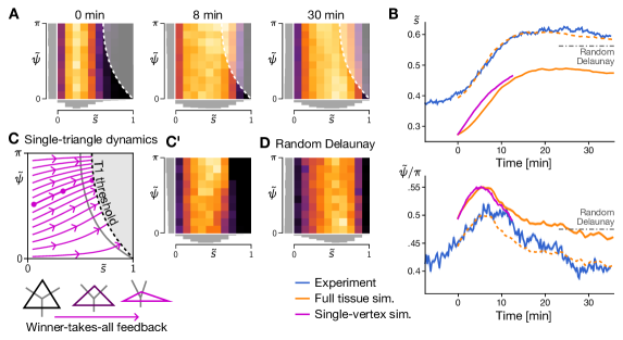
Figure 5: Dynamics LTC order in simulations and the Drosophila germ band. A Heat maps showing the distribution of local tension configurations in a simulation with imposed isogonal strain matching the experimental observations. Data aggregated from $N=6$ simulation runs of $\sim 10^{3}$ cells each. B Driven by winner-takes-all feedback, the magnitude of tension anisotropy magnitude $\tilde{s}$ (top) and the tension bridge fraction (measured by the LTC phase $\tilde{\psi}$l; bottom) increase. The bridge fraction decreases as the tissue becomes disordered due to cell rearrangements. Solid lines show the median of the LTC distributions where the phase $\tilde{\psi}$ is weighted with the magnitude $\tilde{s}$. The width of bands showing the standard error is comparable to the line width. Shifting the median from simulations by a constant offset (see dashed orange lines) yields a quantitative match to the experimental data. C Shape dynamics of a single tension triangle driven by winner-takes-all feedback rapidly drives the tensions towards the T1 threshold with a slight bias towards tension bridges. C’ LTC distribution predicted by single-triangle simulation reproduces the LTC distribution at the onset of cell rearrangements in full tissue simulations (cf. distribution at 8 min in A). D A random Delaunay triangulation seeded from hard disks with a packing fraction $\rho=0.2$ reproduces the late-time distribution in simulations.

With the LTC order parameter and the T1 threshold in hand, we can now quantify the dynamics of tensions in the simulations (see Fig. 5A) and experiments (see companion paper Ref. [17] and Fig. S2). Because isogonal strain shifts the T1 threshold, it will have a significant effect on the LTC order parameter distribution. We therefore performed simulations where we impose the isogonal strain observed in the Drosophila germ band [17]. The germ band is stretched by the invagination of the adjacent mesoderm tissue causing isogonal strain along the axis of tension anisotropy (dorsal–ventral). This shifts the T1 threshold towards stronger tension anisotropy $\tilde{s}$ (cf. Fig. 4E).

At the beginning of the simulation, the local tension anisotropy $\tilde{s}$ is small and there is no bias towards cables or bridges. Positive tension feedback amplifies local anisotropy and thus drives the tension configurations towards the T1 threshold (Fig. 5A). At the onset of T1s, we observe an increased fraction of tension bridges, in agreement with the experimental observations (8 min in Fig. 5A). At late times, where the tissue becomes highly disordered, the distribution in LTC space shifts more towards tension cables (30 min). As we will see below, this late time distribution is reproduced by a random Delaunay triangulation. Time traces of the median anisotropy $\tilde{s}$ and (weighted) median LTC phase $\tilde{\psi}$ show qualitative agreement with data from the Drosophila germ band [17], see Fig. 5B. In fact, a quantitative agreement can be achieved by shifting the median anisotropy and LTC phase by constant offsets, as indicated by the dashed lines in Fig. 5B. These offsets may be a consequence of noise in the experimental data, which we support in Fig. S7 with simulations that incorporate Langevin noise in the tension dynamics.

To understand how tension bridges emerge transiently, consider the shape dynamics of a single, isolated tension triangle governed by winner-takes-all feedback Eq. (5). Starting from a configuration with nearly equal tensions, i.e. a nearly equilateral tension triangle, winner-takes-all feedback causes the highest tension (longest edge in the triangle) to grow at the expense of the other two. The triangle is thus driven towards an increasingly obtuse shape, as illustrated in Fig. 5C. Visualizing this dynamics as a flow in LTC space, shows that it drives the tension configurations towards the T1 threshold and thereby causes the cell rearrangements. The single-triangle simulation successfully predicts early dynamics of the LTC distribution until the onset of cell rearrangements (see Fig. 5B, C’). While positive tension feedback explains the emergence of tension bridges at the single-vertex level, it is not enough to produce an alternating pattern of tensions across cells. This pattern requires that the elementary tension configuration motifs (bridges) fit together coherently, i.e. their tension anisotropy is aligned across cells. This requires that the coordination number of a majority of cells is 6, i.e. that most cells are hexagons. This explains why hexagonal packing order is required to drive coherent T1s that underlie rapid convergent extension.

For a highly ordered initial packing, i.e. a nearly hexagonal lattice of cells, the lattice orientation relative to the axis of mean tension anisotropy determines the initial fraction of tension bridges. It is maximal when one side of the hexagonal cells is parallel to the orientation of tension anisotropy and minimal when one side is perpendicular (see Fig. S6). In simulations we find that this initial bias only weakly affects the initial rate of tissue extension and has no significant effect at later times.

In the simulation discussed above we imposed isogonal strain to account for the transient stretching of the germ band by the invaginating mesoderm. In simulations without imposed isogonal strain, the bridge fraction does not transiently increase (see Fig. S7). This is because the T1 threshold is at a significantly lower anisotropy for tension bridges than for tension cables and this difference is more pronounced for vanishing isogonal strain, causing tension bridges to be rapidly eliminated by T1s (see gray line in Fig. 5C). We therefore predict that T1s will happen at a lower tension anisotropy (and lower tension-bridge fraction) in a tissue with no isogonal strain, e.g. in a twist mutant embryo where mesoderm invagination is abolished.

Loss of order in local tension configurations.

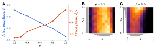
Figure S3: LTC distribution for the hard-disk Delaunay family of random triangulation. A  Median LTC parameter magnitude and phase vs hard disk packing fraction. B, C LTC histograms for two different packing fractions shows significant differences in the LTC distribution for different $\rho$. Note that topological statistics such as coordination numbers are much less sensitive to $\rho$. LTC distributions computed from meshes with $4000$ cells.

Above, we have seen that the cell array becomes disordered as cells rearrange. The coordination number statistics and average shape index approach a random Voronoi tessellation (cf. Fig. 2E, F). This suggests that we can characterize the the corresponding tension triangulations as random Delaunay triangulations. Their statistics of such a triangulation depend on the underlying stochastic point process. We use the same hard disk sampling method as above, controlled by the packing fraction $\rho$ to generate a family of Delaunay triangulations. The triangle shape statistics (characterized by the LTC parameter) found at late times both in simulations and in the Drosophila germ band are reasonably well reproduced by a random Delaunay triangulation seeded from a hard disks with $\rho\approx 0.2$ (Fig. 5D, D’ and Fig. S3). This observed “randomization” in tension space suggests that the triangle edge flips can be statistically understood as a random “mixing”. Notably, the late-time distribution exhibits a bias towards tension cables. The loss of tension bridges causes active T1s to become incoherent and incompatible between adjacent cells, contributing to a slowdown of tissue extension found in tissue scale simulations and in the germ band [17].

Taken together, we find that the time course of LTC distribution agrees between the model and the experimental data. Next, we show how changing various aspects of the model affects the LTC distribution, highlighting that the LTC parameter can be used to distinguish different tension dynamics based on statistical signatures of cell-scale observations.

Saturating tension feedback leads to tension cable formation and reduced convergence extension.

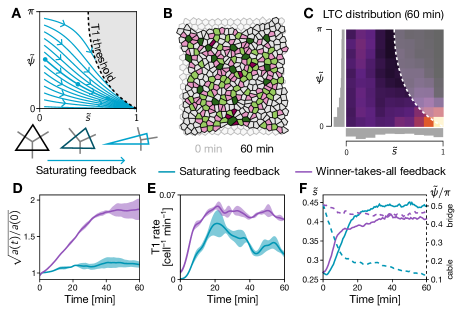
Figure 6: Saturating tension feedback causes tension cable formation and, hence, fails to drive convergent extension. A Local tension configurations are driven towards tension cables due to saturation of positive feedback. Compared to winner-takes-all feedback, this resulting tension dynamics is significantly less efficient at the local configuration towards the T1 threshold (cf. Fig. 5C). B In a tissue simulation, saturating feedback generates only little convergent extension (quantification in D). The initial configuration is shown semi-transparent in the background. Cell color indicates coordination number (cf. Fig. 2A) C The late-time LTC distribution shows a strong cable bias and differs significantly from the random Delaunay distribution emerging in simulations with winner-takes-all feedback (cf. Fig. 5D. D–F Time series quantifications showing that saturating feedback (teal), compared to winner-takes-all feedback (purple), yields very little aspect ratio change (D), a significantly reduced T1 rate (E) and a strongly increased fraction of tension cables (F). Note that in contrast to Fig. 5, the simulations were performed without an imposed isogonal strain such that no significant formation of tension bridges is observed for winner-takes-all feedback.

So far, we used a “winner-takes-all” local tension feedback mechanism, Eq. (5), which drives the formation of tension bridges as illustrated in Fig. 5C. In contrast, when positive feedback rapidly saturates, adjacent high tension interfaces no longer compete, thus leading to the formation of tension cables (Fig. 6A; see SI Sec. II.3 for details). The trajectories in LTC space obtained from single-triangle simulations show that saturating feedback is less efficient at driving the local tension configuration towards the T1 threshold. Indeed, tissue scale simulations with such feedback produce very little convergent extension (see Fig. 6B, D and Movie 3). The rate of T1 transitions is significantly reduced (Fig. 6E), and in contrast to “winner-takes-all” feedback, a significant portion of T1 transitions (approximately 20%) is reversible, i.e. the newly formed edge rapidly re–collapses (see SI). Reversible T1s, which have been observed in certain mutant genotypes [34], can therefore emerge due to altered local tension dynamics. Furthermore, the LTC distribution develops a significant bias towards tension cables (Fig. 6C, F). More generally, this suggests that flow in LTC parameter space, obtained from single-triangle simulations, predicts the efficiency of a given tension-feedback laws at driving T1s.

Tension-triangulation model reproduces Drosophila axis elongation in a simplified geometry

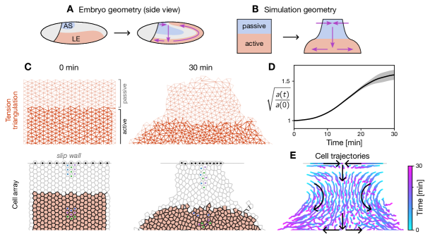
Figure 7: Combining active and passive tissue regions. A, B The ellipsoidal geometry of the Drosophila embryo (A) is mimicked by a simplified simulation geometry corresponding to an unrolled cylinder (B), whose azimuthal axis corresponds to the dorso-ventral (vertical) axis of the embryo. The different behaviour of the dorsal amnioserosa (AS) and the lateral ectoderm (LE) tissue is represented by the passive and active region in the simulation domain respectively. C Positive feedback in the active region amplifies an initial DV anisotropy of tension and thus drives extension along the AP axis. Since the embryos circumference is fixed (implemented via a slip wall at the dorsal boundary), the passive region is stretched along the DV axis. Only half of the simulation domain is shown, corresponding to one lateral side of the left-right symmetric embryo. Three-by-three patches of cells are highlighted to show cell rearrangements (cf. Movie 3). D Tissue deformation, as measured by the change in aspect ratio of the active region, $a(t)/a(0)$, stalls after an elongation (and perpendicular contraction) by a factor $\sim 1.6$. Shading indicates standard deviation over $N=3$ simulation runs of $N_{\mathrm{cells}}\approx 750$ cells. E Trajectories of cell centroids showing the tissue scale flow, resembling the characteristic flow of Drosophila germ-band extension [2].

So far we have considered a patch of active cells with free boundary conditions. However, the epithelium of the early Drosphila embryo forms a closed surface that is approximately an elongated ellipsoid. Therefore, deformation of one tissue region has to be compensated by an opposite deformation of another region. For example, on the Drosphila embryo, the dorsal amnioserosa is passively stretched along the dorso-ventral (DV) axis and compressed along the anterior-posterior (AP) axis to compensate the convergence extension of the germ band. In the following, we investigate the interplay of active and passive tissue deformations.

To mimic the cylindrical geometry of the embryo’s trunk (Fig. 7A) we simulated a rectangular tissue patch with “slip walls” at the top and bottom boundary (Fig. 7B). Along the slip walls, cell centroids, marked by black disks, are restricted to move along the wall. These boundary conditions fix the DV extent of the tissue, corresponding to the fixed circumference of the embryo. We divide the tissue into active and passive regions to account for the different mechanical properties of the lateral ectoderm and the dorsal tissue which becomes the amnioserosa [2, 17]. (The simulation domain is mirror symmetric with respect to the $x$-axis, corresponding to the left-right symmetry of the embryo.) Cortical tensions are governed by positive feedback in the active region and by tension homeostasis in the passive region. Further, passive cells (subscript $p$) are taken to be soft $\mu_{p}=0.2\mu_{a},\;\lambda_{p}=0.2\lambda_{a}$ compared to active cells [35]. In addition, we allow interface angles in the passive region to slightly deviate from those imposed by the tension triangulation, reflecting the fact that the overall scale of cortical tensions is lower in the passive tissue [2]. We initialize the simulation with a slightly perturbed hexagonal packing of cells (motivated by the experimental observations, see Fig. S1) and the experimentally observed tension anisotropy aligned along the DV axis [17].

Starting from this initial condition, the simulation reproduces salient features of the tissue-scale dynamics in the embryo (see Fig. 7C and Movie 3). In the active region (“lateral ectoderm”) active cell rearrangements drive tissue extension along the AP axis and contraction along the DV axis. The passive region (“amnioserosa”) is stretched along the DV axis, accommodating the fixed circumference of the embryo. Notably, this stretching leads to T1s in the passive region as is visible from the highlighted cells in Fig. 7C. On the tissue level, the coupling of active and passive regions gives rise to the tissue flow pattern characteristic of Drosophila germ-band elongation [2] as shown in Fig. 7E.

Tissue extension by active T1s requires large-scale mechanical patterning and cell shape elasticity

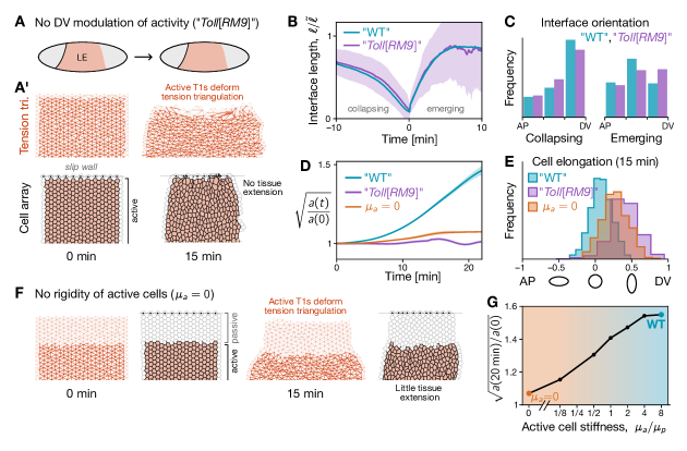
Figure 8: Tissue flow requires cell rigidity and large-scale genetic patterning. A Cartoon of an an embryo without dorso-ventral mechanical patterning, such as a Toll[RM9] mutant where cells all around the circumference adopt a lateral ectoderm (LE) fate. A’ Simulation of a tissue patch without a passive region. While active T1s deform the tension triangulation (top), the cell array (bottom) is blocked from elongating by the fixed DV “circumference” (implemented via slip walls). Instead, cell rearrangements are compensated by isogonal cell elongation (quantified in E), leading to a build-up of elastic energy. B The length dynamics of collapsing and emerging interfaces do not significantly depend on whether the tissue as a whole deforms (WT) or is blocked from undergoing convergent extension (no DV modulation). Purple band shows one standard deviation. Time 0 is the moment of interface collapse. C Orientation of collapsing and emerging interfaces showing that only the orientation of the latter is qualitatively affected by tissue-scale modulation of activity. The orientation of emerging interfaces is slightly biased along the DV direction in the absence of a passive tissue, while it is biased in AP direction in the WT case. D Convergent extension is strongly suppressed in absence of DV modulation of activity (“No DV”) and when active cells have vanishing shear modulus ($\mu_{a}=0$; see F and G). $a(t)$ measures the aspect ratio of the active tissue region. E Histograms of cell shape elongation measured by relative difference, $(S_{\text{DV,DV}}-S_{\text{AP,AP}})/(S_{\text{DV,DV}}+S_{\text{AP,AP}})$, of the AP-AP and DV-DV components of the shape tensor $S$. In the WT case (cf. Fig. 7), cells remain nearly isotropic while they become significantly oriented along the DV axis when DV modulation of activity or rigidity of active cells are abolished. F When the active cells have no shear rigidity ($\mu_{a}=0$), cell rearrangements are compensated by isogonal cell elongation (quantified in E) without incurring an elastic energy build-up. Thus, almost no tissue scale convergent-extension takes place. G Net amount of convergent extension as a function of the shear modulus of active cells shows that active cells need to be stiffer than the surrounding passive tissue for active T1s to drive efficient convergent extension.

The total tissue extension found in the simulations that combine active and passive tissue regions is smaller than the extension of active tissue patches with free boundaries (compare Fig. 7D and Fig. 2C). This suggests that the passive tissue resists deformation. Indeed, cells in the active region are slightly elongated along the DV axis, indicating that the passive tissue pulls on them. In the following, we further investigate the role of the spatial modulation of the cells’ mechanical properties along the DV axis. Figure 8A’ shows a simulation without DV modulation where all cells are active. Positive tension feedback drives active T1s everywhere, as is manifest in the deformation of the tension triangulation (Fig. 8A’, right). However, because of the slip-wall boundary conditions, the tissue cannot contract along the DV axis so that T1s do not result in convergence extension (see Movie 4; quantification in Fig. 8D). Instead, cell rearrangements are compensated by isogonal deformations resulting in elongated cell shapes (as quantified in Fig. 8E). We predict that this scenario will be realized in Toll[RM9] mutant embryos where all cells around the embryo’s circumference adopt a ventro-lateral fate [27], as illustrated in the cartoon in Fig. 8A.

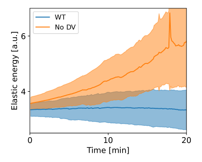
Figure S9: Elastic energy in germ-band simulations tissue-scale simulations (Fig. 7). Note that in “WT” simulations, the elastic energy does not increase over time. If no passive tissue exists to compensate the extension of the germ band, cell elongate and elastic energy builds up.

The stretching of cells leads to a buildup of elastic energy (see Fig. S9). Eventually the increasing frustration leads to convergence issues in the numerical simulation for $t\gtrsim 20\;\mathrm{min}$. In Toll[RM9] mutant embryos, some of this elastic energy is released by the formation of folds (buckling) [27] which our 2D simulations cannot capture. A partial compensation of cell rearrangements by cell shape changes might be observed in the germ band of mutants where the soft amnioserosa is abolished (e.g. in dpp[hin46] mutants).

An interesting observation from the above simulations is that the length dynamics of collapsing and emerging interfaces is not significantly affected by the lack of tissue-scale mechanical patterning (Fig. 8B), even though there is no tissue extension. Interface elongation in the absence of tissue elongation has previously been observed in experiments where germ band extension has been blocked by cauterization near the posterior pole [8, 36]. We mimic the experiments of Ref. [8] by adding slip walls to the anterior and posterior boundary of the simulated tissue (Fig. S8) to block tissue extension. In this scenario, we also observe that newly formed interfaces extend, but with a slightly different dynamics than in WT. In further agreement with experimental observations, we find that the orientation of extending interfaces is no longer biased along the AP axis when tissue extension is blocked (see Fig. 8C). Since interface extension in our model is a purely passive process, we conclude that no active mechanisms – such as medial myosin pulses [8] – are necessary for the elongation of new interfaces. Instead, interface elongation results from the fundamental temporal asymmetry of the intercalation process, i.e. the low level of active tension on the new interface (see companion paper [17]).

Rather than abolishing the DV modulation of activity, one can also change the passive elastic properties of the cells. Recall that in the model, the resistance of cells against deformations is described by the cell-shape elastic energy, Eq. (3) parameterized by the Lamé coefficients $\lambda$ (resistance to area changes) and $\mu$ (resistance to shear deformation). Fig. 8F shows a simulation where the shear modulus $\mu_{a}$ of active cells is set to zero, so that the cells do not resist (area-preserving) elongation. Active T1s can therefore be fully compensated by cell elongation through isogonal deformations without incurring an elastic energy. As a result, there is no net tissue deformation (see Movie 4). In other words, cell-shape rigidity is required to maintain rotund cell shapes (i.e. resist isogonal shear deformations) and thus translate active T1s into net tissue deformation. The tissue deformation by isogonal modes is determined by a a balance of external forces and internal resistance of cells the shape changes. Here, the external forces acting on the active tissue result from the passive tissue’s resistance to deformation, which is in turn set by shear modulus $\mu_{\mathrm{p}}$. The ratio of the shear moduli in the active vs the passive region, $\mu_{\mathrm{a}}/\mu_{\mathrm{p}}$, determines how much the active region deforms (see Fig. 8G). Only when the cells in the active tissue are more rigid than those in the passive region ($\mu_{\mathrm{a}}/\mu_{\mathrm{p}}>1$), is it energetically favorable to isogonally deform the passive region rather than the active region. This predicts that GBE can be impaired by stiffening the dorsal tissue (amnioserosa).

Discussion

We formulated a cell-scale model for epithelial tissue dynamics based on the assumptions of adiabatic force balance in the regime of dominant cortical tensions. Experimental evidence [37, 22, 17] suggests that the cortical cytoskeleton which generates this tension behaves more like a muscle, where the tension level is set by active regulation, rather than a spring, where tension is a function of length. Subscribing to these assumptions has two important consequences: First, feedback loops are required to achieve and stabilize a force-balanced configuration [13]. This is in contrast to a network of springs where the relation between length and tension (the constitutive relationship) ensures that force balance is reached by minimization of the elastic energy. Second, force balance of cortical tensions does not fully constrain the tissue as is allows for isogonal (angle-preserving) deformations which change the lengths of interfaces without changing the angles at which they meet in vertices [13]. These isogonal degrees of freedom of the cortical network are governed by non-cortical mechanical stresses, arising e.g. from passive cell elasticity, representing cell-internal structures such as the nucleus [20], microtubules, and intermediate filaments [21]. We find that this internal rigidity is essential to transduce cell intercalations into tissue-scale deformation. In the absence of cell resistance against deformation, intercalations are compensated by cell shape changes. Our findings suggest that epithelial tissue flows not like a fluid (where the shear modulus vanishes) but rather as a plastically deforming solid, whose remodeling is driven internally while resisting external forces. Epithelial tissue can thus be regarded as an active solid.

Our model formulates a theory of active elasticity where the dominant (cortical) stresses are not governed by constitutive relationships. It builds explicitly on the geometric relation (duality) between tension space and real space afforded by the force balance condition. Stabilizing feedback mechanisms that maintain adiabatic force balance are implicit in our model as we constrain the tension dynamics to the space of force-balanced configurations (flat tension triangulations). Tension dynamics is formulated as geometric dynamics of the tension triangulation driven by local positive feedback. This feedback amplifies a weak initial tension anisotropy and thus drives cell shape dynamics that result in cell intercalations (T1 processes). Force balance provides the non-local coupling that allows for coordination of forces and cellular behaviors across the tissue. On the tissue scale, self-organized active T1s are oriented by global tension anisotropy and thus drive convergent–extension flow. As T1s drastically remodel tension geometry, they gradually degrade the orientational cue provided by initial tension anisotropy. Thus, tissue flow arrests after a finite extent of convergent extension that depends on the initial degree of order in the cellular packing and the magnitude of initial tension anisotropy. This central finding suggests that cell geometry is a repository of morphogenetic information that may encode the final tissue shape.

Mechanically self-organized tissue dynamics provide an elegant explanation of Drosophila germ band elongation and its arrests after about two-fold elongation. Importantly, geometrically formulated tension dynamics can be directly compared with experimental data on the cell scale [17]. To this end, we have introduced the LTC order parameter for the local configuration of tensions. Comparing the LTC time courses between experiments and simulations, we find excellent agreement, suggesting that our model reproduces the dynamics of germ band extension also on the cell scale. Specifically, our order parameter distinguishes two motifs of local tension configurations “tension cables” where multiple high tension interfaces meet in a vertex and “tension bridges”: high tension interfaces surrounded by low tension interfaces. Tension bridges are the elementary motif of the alternating pattern of tensions that choreographs active T1s across the tissue.

The dynamics in tension configuration space depends on the nature of the positive tension feedback. Winner-takes-all feedback efficiently drives the local tension configuration toward the T1-threshold via the formation of tension bridges. By contrast, when feedback saturates at too low relative tension, it causes formation of tension cables, which have previously been suggested as a driver for convergent extension. However, our simulations and analysis of local tension configurations show that tension cables are inefficient at driving convergent extension, as adjacent interfaces “compete” to contract. Indeed, arrest of convergent extension due to the formation of tension cables is also observed in a recent computational study [10]. Contraction of tension cables leads to formation of “rosettes” where five or more cells meet in a single vertex. While it has been suggested that rosettes are important for epithelial convergent extension [37, 38], recent whole-embryo analysis of Drosophila gastrulation [17, 16] shows that rosettes contribute significantly less to tissue extension than T1s and appear in conjunction with disorder which arrests tissue flow. Our simulations corroborate these empirical findings. Moreover, tension cables are often found to form at boundaries between distinct tissues and at segment boundaries where they prevent mixing between the adjacent tissues, i.e. prevent cell rearrangements [39, 40, 41, 42]. In contrast to tension cables, which clearly stand out in microscopy images (e.g. of fluorescently labelled myosin), tension bridges are hard to spot as they rapidly contract. This might be a reason why the role of tension bridges has not been appreciated before. The tension configuration parameter introduced here facilitates a statistical analysis across many cells and allows one to distinguish different local tension dynamics (e.g. winner-takes-all vs saturating feedback).

Our scenario for GBE is based on local self-organization driven by mechanical feedback. Self-organized T1s are facilitated by the initial order in the cell packing and are oriented by an initial global tension anisotropy but do not require cell-scale genetic instructions [27, 43]. We expect that this tension anisotropy, whose presence we confirmed experimentally in Ref. [17], is due in part to the anisotropic static “hoop” tension resulting from the internal turgor pressure in the embryo, and to the dynamic effects of ventral furrow formation [14]. To create global tissue flow, local self-organization must be modulated by large-scale pre-patterning of cell behaviors. In the early Drosophila embryo, this is manifested in the dorso-ventral patterning system that specifies the tissues with different mechanical properties and modulates mechanical feedback loops [14]. Classical work shows that the direction of GBE can indeed be reversed by flipping the orientation of DV patterning [44]. In simulations on a cylindrical geometry without droso-ventral patterning, mimicking a Toll[RM9] mutant, active T1s occur in the absence of tissue flow. Instead, the cell rearrangements are compensated by cell shape deformations. Notably, these simulations also show that T1 resolution does not require isotropic contractions of the cells’ apical area by “medial” myosin pulses [8]. Taken together, our model provides unified picture for Drosophila GBE that bridges the cell and tissue scales. The integration of bottom-up self-organization and top down genetic control emerges as a common theme in development [45].

Our model predicts that disrupting the hexagonal packing of nuclei prior to cellularization will cause slower GBE. Interesting candidates to test this prediction are “nuclear fallout” mutants where some nucelei leave the blastoderm surface and thus introduce defects in the cellular packing [46]. Another option might be the transient and partial disruption of microtuble organization with small molecule inhibitors [47]. We expect that these experiments can be used to challenge and subsequently refine the model.

An important challenge for future work is to identify the (molecular) mechanisms that stabilize the force-balanced configuration on short timescales while driving controlled remodeling on long timescales. In our model, maintenance of force balance was achieved via the “flattening” of the tension triangulation which subsumes the complex regulatory feedback loops operating in the cortical cytoskeleton. The underlying mechanics of the interplay of actin fibers, myosin motors, passive crosslinkers (such as spectrins [48]) and mechanical feedback mediators (such as $\alpha$-catenin [49]) remain poorly understood. We hope that the insights from the geometrical model and the quantification of local tension configurations [17] will help develop more fine-grained models that explicitly account for these details.

Finally, a general open problem is coarse-graining of discrete tissue models to a continuum theory. The geometry of the tension triangulation and isogonal modes may provide a fruitful new perspective on this problem. Such future efforts will also help make contact between adiabatic remodeling of tensions in force balance and existing continuum models of tissue dynamics that are based on viscoelasticity, where active stress are balanced by viscous dissipation and friction [1, 2, 50].

Supplementary Material

I Analysis of experimental data

I.1 Experimental data source

Whole embryo cell segmentation and tracking data was obtained from the repository DOI:10.6084/m9.figshare.18551420.v3 deposited with Ref. [16]. We analyzed the dataset with ID number 1620 since it had the highest time resolution ($15\text{\,}\mathrm{s}$) and covered the longest time period ($50\text{\,}\mathrm{min}$), starting ca. $7\text{\,}\mathrm{min}$ before the onset of ventral furrow invagination.

I.2 Hexagonal packing and hexatic order

We quantify order of the cell arrangement in the tissue by two measures: (i) the fraction of six-sided cells, that one might loosely call “hexagonal packing order” and (ii) the hexatic order parameter measuring bond-orientational order. Hexagonal packing order is a topological quantity – it depends only on the neighborhood relations between cells but not on their exact shape. In contrast, hexatic order (defined below) is a geometric measure, that is sensitive to the cell shapes. Initially, the majority of cells have six neighbors (Fig. S1A, 0 min), and the density of topological defects, manifested as non-hexagonal cells, is relatively low. During VF invagination, the number of defects increases only slightly (25 min) since there are only very few intercalations [17]. During GBE, the number of defects increases significantly as a consequence of T1s. Towards the end of GBE, the distribution of cell-coordination number approaches that of a random Voronoi tessellation seeded with a Ginibre random point process (see Fig. S1B and B’).

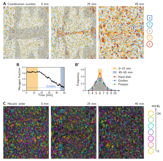
Figure S1: Coordination number and hexatic order of cells. A Initially (0 min), the majority of cells are hexagonal (light gray). During GBE (25–50 min), topological defects proliferate, resulting in increasing numbers of non-hexagonal cells. Semitransparent gray overlay marks cells that invaginate. B and B’ Fraction of hexagonal cells as a function of time (B) and histogram of cell-coordination number (B’) in the lateral ectoderm. The histograms show pooled data from the time periods 0–15 min and 45–50 min highlighted in B. Lines indicate the coordination number distributions for Voronoi tessellations generated from three different random point processes: hard disk (packing fraction 0.54 near the theoretical maximum for sequential placement [51]), Ginibre [52], and Poisson. C Hexatic order is low, and shows no long-range correlation. It further decreases as GBE progresses. Hue and brightness code for the phase ($\mathrm{arg}\,\psi_{6}$) and magnitude ($|\psi_{6}|$) of the hexatic order parameter, respectively.

Hexatic order.

The hexatic order parameter (also called “bond orientational order parameter” [53]) for a cell with $n$ vertices is defined as

$$\psi_{6}=\frac{1}{n}\sum_{k=1}^{n}\exp(6i\theta_{k}),$$ (12)

where $\theta_{k}$ is the angle between the DV axis and the vector pointing from the cell’s centroid to vertex $k$. For a cell with regular hexagonal shape the magnitude of $\psi_{6}$ reaches its maximum $|\psi_{6}|=1$. The phase $\mathrm{arg}\,\psi_{6}$ indicates the orientation of the hexagon. In contrast to the coordination number, which is a purely topological measure, the hexatic order parameter depends on the cell shape. We find that the hexatic order parameter to be low in magnitude and exhibit no long-range correlations as is apparent from Fig. S1C. Effectively, the presence of non-hexagonal cells act as obstructions to long range correlations of geometric order. We quantify the range of correlations in hexatic order by coarse graining over patches of cells with different radii (measured in the by the neighborhood degree). Before the onset of GBE, the coarse grained order parameter decays as a power law of the patch radius law with an exponent that close to $-0.75$, a value found also for MDCK cells and in simulations using multiphase-field models [54]. (We find the same result using the distance-weighted hexatic order parameter introduced in Ref. [54].) At the end of GBE, the decay exponent is smaller than $-1$, indicating a complete lack of correlations in hexatic order between neighboring cells. This is expected from the high number of non-hexagonal cells at this stage (Fig. S1B, 50 min).

I.3 Local and regional tension inference

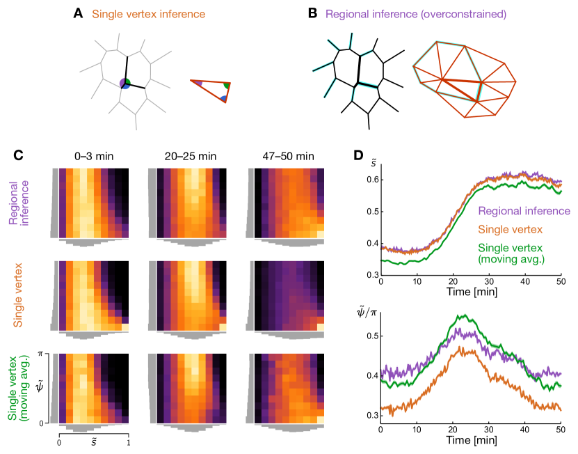
Figure S2: Comparison of local vs regional tension inference. A Local tension inference at a single vertex through complementarity of angles at a single vertex (left) and in the corresponding tension triangle (right). The relative tensions (edge lengths of the tension triangle) are found via the law of sines. B Regional tension inference for a patch of three cells. The interfaces (and corresponding tensions) shared between them are highlighted by bold lines. The triangulation property of the tensions yields one additional constraint for each cell because for each cell there is a loop in the tension triangulation which has to close. One such loop is highlighted. These additional constraints make the regional inference more robust. C Comparison of the LTC distributions for regional and local tension inference in the Drosophila germ band. Distributions are from data collected over the indicated time intervals. Germ band elongation starts at ca. 25 min. The last row shows single-vertex inference based on vertex positions smoothed using a moving average (1.25 min interval). D Mean anisotropy magnitude (top) and LTC phase (bottom) for the three inference variants. Note the systematically lower LTC phase, i.e. lower fraction of tension bridges, found using single-vertex inference.

To quantify the local tension configurations in experimental data from the Drosophila germ band, we performed tension inference based on segmented cell outlines. In the companion paper [17], tension inference was done locally, directly relating the angles at each vertex to the relative cortical tension via the law of sines (see Fig. S2A). While this method is conceptually and computationally simple, it is sensitive to observational and dynamical noise in the angles. A more robust approach is to perform tension inference in an extended region, which makes the inference problem overconstrained [13]. In particular, there is one additional constraint per cell because the tension triangles for each cell have to fit together in force balance as illustrated in Fig. S2B. The overconstrained inference returns tensions for the closest force-balanced configuration compatible with the observed angles and thus removes small deviations from tensional force balance due to pressure differentials, short-time fluctuations, and observational noise. (An alternative method to remove observational noise is to apply a moving average on the vertex positions before inferring tensions.) Since in our model cortical tensions are always in exact tensional force balance, we use this overconstrained inference to compare to simulations. Specifically, we use tension inference on all interfaces of the three cells which meet at a given vertex to determine the local tension configuration parameter at that vertex. Figure S2C shows the LTC distributions obtained from local and regional inference. The LTC distributions are qualitatively very similar but they differ quantitatively. In particular, the LTC phase $\tilde{\psi}$ has the same qualitative trend with a transient increase before the onset of T1s but is systematically lower for regional inference.

II Additional simulation results

In this section we report additional results from the tissue scale simulations and/or explain implementation details.

II.1 Influence of isogonal stretching on the LTC distribution

Here, we consider the influence of the reference cell shape $S_{0}$ which determines the isogonal potential via the elastic energy. As discussed in the main text, isogonally stretching or compressing cells along the axis of tension anisotropy can delay or accelerate T1s by moving the T1-threshold in LTC space. As reported in the main text, if we implement isogonal stretching by choosing an anisotropic $S_{0}$, i.e. $S_{0}=3\ell_{0}\;\mathrm{diag}(1-t,1+t),\;t\in[0,1]$, we find that that a higher bridge bias emerges at the early phase of convergent extension (Fig.5). We chose an anisotropic reference shape $t=1/3$ to model the isogonal stretching caused by the ventral furrow before onset of GBE. In the experimental data, this isogonal stretch decays; analogously, we linearly ramp the reference shape anisotropy down so that $t=0$ at 50 minutes simulation time. We note that our modelling of isogonal stretching is limited, since it is encoded in a model parameter ($S_{0}$) instead of being created dynamically, for example by external forces applied to the boundary. Time traces of the LTC parameter in the absence of isogonal stretching are show in Fig. S7) below.

II.2 Alternative forms of positive tension feedback

We now turn to discussing two variants of the triangle-intrinsic tension dynamics. In the main text, we discussed two types of positive feedback, saturating and winner-takes-all. In both cases, the overall scale of tensions was determined by keeping the triangle perimeter $P=\sum_{\alpha\in I_{ijk}}\tilde{T}_{\alpha}$ constant. This corresponds to a fixed amount of total active tension that is only redistributed across edges. We can also consider a model where the triangle area remains fixed. This can be implemented using the gradient $(J_{A})_{ij}=\partial_{\tilde{T}_{ij}}A_{I_{ijk}}$ of the triangle area:

$$\partial_{t}\tilde{T}_{ij} ={\tau_{\mathrm{T}}}^{-1}\left(\tilde{T}_{ij}^{n}-\frac{1}{||\mathbf{J}_{A}||}\sum_{\alpha\in I_{ijk}}(\partial_{\tilde{T}_{\alpha}}A_{I_{ijk}}\tilde{T}_{\alpha}^{n})\right)$$ (13)

The overall dynamics of this model is very similar to Eq. 5 considered in the main text. However, the tension feedback is “more aggressive” since now the total tension (triangle perimeter) increases as the tension triangle becomes more anisotropic. This mirrors a situation where in addition to the anisotropy also the total myosin levels increase during GBE [55]. Therefore, one observes slightly larger amounts of convergent extension for identical initial conditions.

Next, we considered adding small amounts of i.i.d. Gaussian noise to the cortical tension dynamics, i.e. a stochastic, Langevin tension evolution

$$\tau_{\mathrm{T}}\partial_{t}\tilde{T}_{ij}=\tilde{T}_{ij}^{n}-\frac{1}{3}\sum_{\alpha\in I_{ijk}}\tilde{T}_{\alpha}^{n}+\eta_{ij},$$ (14)

$$\text{with}\;\eta_{ij}\sim_{\text{i.i.d.}}\text{Normal}(0,\sigma^{2})\;\text{and}\;\langle\eta_{ij}(t)\eta_{kl}(t^{\prime})\rangle=\sigma^{2}\delta(t-t^{\prime})\delta_{ij,kl}$$ (15)

To integrate Eq. 14, we use the explicit Euler-Maruyama scheme. We find that the convergent extension phenomenology is robust to low to moderate levels of noise (i.e. $\sigma<T_{ij}^{n}$). However, higher $\sigma$ leads to a final LTC distribution with somewhat more anisotropic triangles, indicating larger disorder, and reduces the amount of total convergent extension.

Meshes from a Langevin simulation and from a simulation with an area-based myosin pool mechanism are shown in Fig. S5. A quantitative analysis is shown in Fig. S7.

II.3 Saturating tension feedback

Here, we present the details for the simulations of saturating tension feedback in main text Fig. 5. We consider bistable tension dynamics of the form

$$\tau_{T}\frac{d}{dt}\dot{T}=-(T-T_{-})(T-T_{c})(T-T_{+})$$ (16)

where $T_{-}<T_{c}<T_{+}$ are the low, unstable, and high tension fixed point, respectively. We set $T_{-}=0,\;T_{c}=1$ matching the fixed points of the main feedback model Eq. (5) we consider in this manuscript. The simulations with saturating feedback correspond to $T_{+}=1.2$, the control simulations are $T_{+}=3.33$. Note that we adjusted the time step and all other rate parameters of the simulation so that $\dot{T}$ is similar across different choices of $T_{+}$.

II.3.1 Irreversible and reversible T1 transitions

We note that in the case of saturating tension feedback, a relevant fraction of T1s (approx. 20%) are reversible, i.e. the newly formed junction re-collapses, which occurs in less than 1% of cases for non-saturating feedback. Only irreversible T1s are counted in Fig. 6E. Because saturating feedback only very rarely produces reversible T1s, all quantifications other than Fig. 6 show the total T1 count without any filtering.

Reversible T1s are defined as follows. Consider an edge $ij$ between cells $i$ and $j$, the central edge in a quartet of cells $ikjl$ (in clockwise order). The collapse of edge $ij$ creates an edge $kl$. This T1 is considered reversible if $kl$ collapses in turn to give rise to a connection $ij$ again, i.e. $kl$ re–collapses before any of the outer edges $il$, $lj$, $ik$, or $ki$, of the quartet have collapsed. In this case, the local quartet topology returns to its original state. We also filter out nested sequences of multiple reversible T1s, but such events are extremely rare.

II.4 Tension-driven Voronoi model

As mentioned in the main text, the only way the real-space vertices $\mathbf{r}_{ijk}$ feed back into the tension dynamics is by determining when a T1 transition, and hence a topological modification of the translation, occurs. Instead of obtaining the vertex positions from angle-constrained minimization of an elastic energy, one can construct them directly from the tension triangulation using the Delaunay–Voronoi duality (vertices of the Voronoi tessellation, $\mathbf{r}_{ijk}$, are the circumcenters of triangles $\mathbf{t}_{i}\>\mathbf{t}_{j}\>\mathbf{t}_{k}$). The resulting tessellation obeys cortical force balance. The Voronoi cell shapes are good approximation to those obtained by minimization of the cell shape energy for an isotropic target cell shape $S_{0}$. In particular, in the Voronoi tessellation a T1 at an edge $ij$ occurs when the sum of the opposing triangulation angles $\phi_{ijk}+\phi_{ijl}>\pi$. This condition is simple to check numerically, whereas the elastic energy minimization is by far the numerically most costly and complicated step in our simulations. The tension-driven Voronoi model therefore defines a computationally efficient model for tension-driven tissue dynamics. For instance, during the construction of the tension dynamics model presented in this paper, we made frequent use of the tension-driven Voronoi model for preliminary numerical experiments. Note that by definition, it is not possible to incorporate isogonal strain in this model, and hence neither passive tissue patches nor fixed boundary conditions can be implemented. Further, in particular for disordered and anisotropic tension triangles, the Voronoi prescription creates cell shapes that differ from those obtained by energy minimization.

Figure S4 demonstrates that for simulations with free boundary conditions, as performed in main text Fig. 2, the tension-driven Voronoi model behave very similar to full elastic energy minimization. A mesh from a tension-driven Voronoi simulation is shown in Fig. S5.

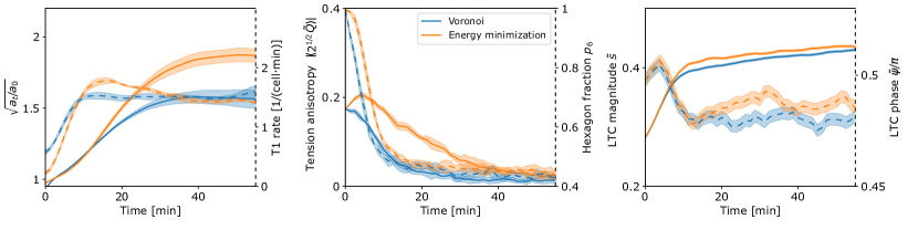
Figure S4: Comparison of the tension-driven Voronoi model where the cell shapes are determined via Voronoi–Delaunay duality from the tension triangulation (blue) vs simulations of the full model where cell shapes are obtained by minimizing the cell shape energy under the angle constraints imposed by the tension triangulation (orange). Simulations were initialized with an “ordered” tension triangulation (generated from hard disks at high packing fraction $\rho=0.9$) and initial tension anisotropy magnitude $s=0.2$. The three panels follow the same convention as Fig. S6B–D.

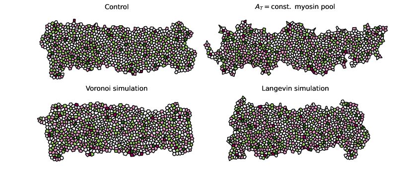
Figure S5: Final tissue shapes (40 min simulation time) for the alternative tissue dynamics models discussed in the SI. Simulations were initialized with an “ordered” tension triangulation and initial anisotropy $s=0.2$. Cells are colored by coordination number (same color code as in Fig. 2A.

II.5 Effect of hexatic order orientation

When carrying out simulations in which the tissue is initially ordered, the initial tension triangulation corresponds to a (rectangular) patch of a triangular lattice. We can choose two possible orientations of the lattice plane with respect to the tension anisotropy – one creating initially mainly tension cables, one mainly bridges. This corresponds to the orientation of the hexatic order $\Psi_{6}$ w.r.t. the axis of tension anisotropy, and we refer to these orientations as “bridge” and “cable” initial conditions. We find that the qualitative behavior of the model is independent of this choice, and positive tension feedback is capable of creating coherently ordered T1s even if future collapsing edges are not singled out in the initial condition. To underline this point, Fig. 2 uses “cable” initial conditions. For the determination of LTC distribution dynamics in main text Fig. 5, we pool simulations from cable and bridge initial conditions. When showing snapshots from a simulation, the “parallel” initial condition most easily creates the recognizable pattern of alternating high and low tensions reported in the companion paper.

A quantitative comparison is shown in Fig. S6. We see that an initial bridge bias leads to higher bridge fraction later on, and somewhat larger amounts of convergent extension.

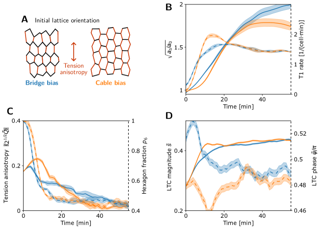
Figure S6: Dependence of tissue dynamics on initial tension bridge vs tension cable bias. A The orientation of a hexagonal array of cells relative to the axis of tension anisotropy determines whether the anisotropic tensions manifest primarily as tension bridges (left) or tension cables (right). B–D Quantification of simulations initialized with hexagonal cell arrays with bridge bias (blue curves) and cable bias (orange curves). B Change of tissue aspect ratio (solid lines, left axis) and T1 rate (dashed lines, right axis) show that convergent extension is faster and more efficient (fewer T1s are required for the same shape change) for an initial bridge bias. Shaded bands indicate standard deviation. C Magnitude of mean tension anisotropy (solid lines, left axis) and hexagon fraction (dashed lines, right axis). Shaded bands indicate standard deviation. D Mean local tension anisotropy magnitude (solid lines, left axis) and median LTC phase (dashed lines, right axis) showing the initial bridge/cable bias and eventual convergence of the LTC phase. Shaded bands indicate standard error. Initial tension anisotropy magnitude $s=0.2$.

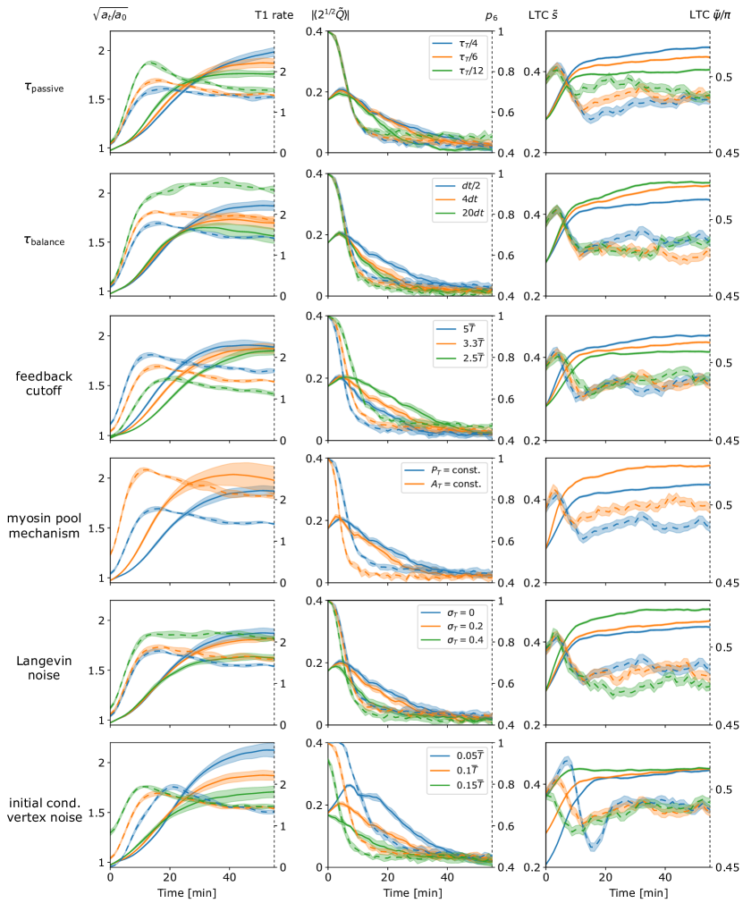
Figure S7: Dependence of model behavior on parameters. Each row of plots shows the dependence on one parameter or modelling choice. The three columns follow the same convention as Fig. S6B–D. The passive relaxation time $\tau_{p}$, the balancing time $\tau_{\mathrm{balance}}$, the feedback cutoff, and the initial condition vertex noise are explained in more detail SI Sec. IV.

II.6 Interface extension is independent of tissue extension

As argued in the main text, interface extension after active T1s is not driven by external forces (e.g. due to tissue elongation) but locally by cortical tensions. Active T1s are fundamentally asymmetric in time: the collapsing interface has high myosin levels, and the newly formed interface has very low levels. Since these low levels are insufficient to balance the tensions of the surrounding interfaces, the new interface extends.

Our simulations support the notion that interface extension does not depend on tissue extension, even though our simulations contain no additional active mechanisms to elongate new interfaces. In the main text, we showed simulations of a tissue geometry without a soft, passive region to compensate the convergence of the active tissue (analogous to a Toll[RM9] mutant). Because of incompressibility, the active tissue also does not extend. Nevertheless, new interfaces elongate at rates very similar to control simulations (Fig. 8). We now support this conclusion with an additional simulation. Mimicking experiments where tissue extension is blocked by a cauterization fence [8], we block tissue extension by adding slip walls along the AP boundaries of the tissue patch (Fig. S8A). For numerical reasons, we add a small passive zone in front of these additional boundaries, and enforce the slip-wall condition with a softer penalty than for the dorsal slip walls. This is done to avoid direct conflicts between the boundary conditions and the angle constraints from the triangulation. In these simulations, the active tissue does not extend, and cells deform to compensate T1s (Fig. S8A). In a control simulations (Fig. 8), by 15 minutes, the tissue has elongated by 30% by the time shown. However, new interfaces still successfully extend (Fig. S8B), like in the Toll[RM9] simulations shown in Fig. 8. The overall speed of intercalations is slightly reduced because of the additional slip walls. Note that occasionally, we observe rupture of the simulated tissue from the simulation boundary because of the internal forces generated by T1 transitions. Similar rupture events are seen in experiment.

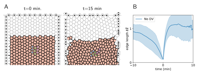
Figure S8: Interfaces extend even if tissue extension is blocked. A Snapshots from a simulation where tissue extension is blocked by slip walls along the AP boundaries of the tissue patch. This mimics experiments where the germ band is blocked from extending via cauterization of the ventral tissue close to the posterior pole, or mutations in the posterior midgut [8]. B Even though net tissue deformation is blocked, the interface length during active T1s is qualitatively similar to simulations of freely deforming tissues (cf. “WT” in Fig. 8B).

III Isogonal shear and tissue shear modulus

As discussed in the main text, and shown in Fig. 8 our simulations show that a non-zero cell-level shear modulus is required for extension via active T1s. Here, we analyze the relation of cell-level and tissue-level shear modulus. Crucially, because of the dominance of cortical tensions, a tissue patch in our model will respond to externally applied forces via an isogonal deformation. We first show that an isogonal deformation can create tissue-scale pure shear (on the level of cell centroid displacement – the transformation of cell vertices is necessarily non-affine to preserve angles). Then we show that these pure shear modes correspond to the response of the tissue to external force by computing the Hessian of our cell elastic energy in the subspace spanned by isogonal deformations, and measure the shear modulus.

III.1 Quadratic isogonal mode profile creates pure shear

To show that isogonal modes can create pure shear, not just dilation/contraction of cells, we make use of the isogonal mode parametrization introduced in Ref. [13]. It assigns an isogonal “potential” $\Theta_{i}$ to each cell, and calculates the cell displacements from the $\Theta_{i}$ and the edge tension vectors. In the following, we will show that a constant gradient in the isogonal potential generates a uniform translation in real space. By integration, this implies that a quadratic spatial profile of the isogonal potential creates a pure shear.

Let us identify the real space edge unit vectors by the two adjacent cells $\mathbf{e}_{ij}=-\mathbf{e}_{ji}$ and denote the corresponding tensions as $T_{ij}$. Then the tension vectors $\hat{\mathbf{T}}_{ij}=T_{ij}\hat{\mathbf{e}}_{ij}$ form a triangulation, where $\hat{\mathbf{a}}$ denotes the normal vector to $\mathbf{a}$, i.e. $\hat{\mathbf{a}}.\mathbf{a}=0$ and $||\hat{\mathbf{a}}||=||\mathbf{a}||$.

The isogonal displacement $\mathbf{u}_{ijk}$ of the real space vertices $\mathbf{r}_{ijk}$ (identified by the three adjacent cells) is given by

$$\mathbf{r}_{ijk}\to\mathbf{r}_{ijk}+\mathbf{u}_{ijk}=\mathbf{r}_{ijk}+\frac{1}{S_{ijk}}\big{[}\Theta_{i}\mathbf{T}_{jk}+\text{(cyc.)}\big{]}$$ (17)

where $S_{ijk}=\hat{\mathbf{T}}_{ij}.\mathbf{T}_{ik}$ is the area of the tension triangle $(ijk)$.

First, observe that the uniform isogonal mode $\Theta_{i}={}$const. has no effect on the vertex positions because

$$\mathbf{T}_{jk}+\mathbf{T}_{ki}+\mathbf{T}_{jk}=0\quad\text{(force balance).}$$ (18)

Now we aim to show that a constant gradient in $\Theta_{i}$ drives a uniform displacement of the $\mathbf{r}_{ijk}$. Specifically, by uniform gradient we mean $\Theta_{i}=\mathbf{t}_{i}.\mathbf{a}$, i.e. a linear gradient in the tension space ($\mathbf{t}_{i}$ is the position of the tension triangulation vertex corresponding to cell $i$, such that $\hat{\mathbf{T}}_{ij}=\mathbf{t}_{j}-\mathbf{t}_{i}$). To show that the displacement in real space is uniform, it is enough to show that two adjacent vertices are displaced identically. By induction, this implies that all displacements are identical. It is therefore sufficient to consider a quartet of cells ($i=1{--}4$), corresponding to a “kite” in tension space (note that $\hat{\mathbf{a}}.\mathbf{b}$ is identical to the wedge product $\mathbf{a}\wedge\mathbf{b}$.)

Because a constant can be arbitrarily added to all $\Theta_{i}$, we can set $\Theta_{1}=0$ and thus have $\Theta_{i}=\hat{\mathbf{T}}_{ij}.\mathbf{a}$ for $i=2,3,4$. The displacements now read

$$\mathbf{u}_{123} =\frac{1}{S_{123}}\big{(}\hat{\mathbf{T}}_{12}.\mathbf{a}\;\mathbf{T}_{31}+\hat{\mathbf{T}}_{13}.\mathbf{a}\;\mathbf{T}_{12}\big{)}$$ (19)

$$\mathbf{u}_{134} =\frac{1}{S_{134}}\big{(}\hat{\mathbf{T}}_{13}.\mathbf{a}\;\mathbf{T}_{41}+\hat{\mathbf{T}}_{14}.\mathbf{a}\;\mathbf{T}_{13}\big{)}$$ (20)

To show that these displacements are identical, we project them onto two conveniently chosen, linearly independent vectors, namely $\hat{\mathbf{T}}_{12}$ and $\hat{\mathbf{T}}_{13}$. For the latter we find

$$\hat{\mathbf{T}}_{13}.\mathbf{u}_{123} =\frac{1}{S_{123}}\hat{\mathbf{T}}_{13}.\mathbf{a}\;\hat{\mathbf{T}}_{13}.\mathbf{T}_{12}=-\hat{\mathbf{T}}_{13}.\mathbf{a},$$ (21)

$$\hat{\mathbf{T}}_{13}.\mathbf{u}_{134} =\frac{1}{S_{134}}-\hat{\mathbf{T}}_{13}.\mathbf{a}\;\hat{\mathbf{T}}_{13}.\mathbf{T}_{14}=-\hat{\mathbf{T}}_{13}.\mathbf{a},$$ (22)

where we used that $\hat{\mathbf{T}}_{ij}.\mathbf{T}_{ij}=0$ and applied the definition of $S_{ijk}$.

Projecting (19) and (20) onto $\hat{\mathbf{T}}_{12}$ gives

$$\hat{\mathbf{T}}_{12}.\mathbf{u}_{123} =\frac{1}{S_{123}}\hat{\mathbf{T}}_{12}.\mathbf{a}\;\hat{\mathbf{T}}_{12}.\mathbf{T}_{31}=-\hat{\mathbf{T}}_{12}.\mathbf{a}$$ (23)

$$\hat{\mathbf{T}}_{12}.\mathbf{u}_{134} =\frac{1}{S_{134}}\big{(}\hat{\mathbf{T}}_{13}.\mathbf{a}\;\hat{\mathbf{T}}_{12}.\mathbf{T}_{41}+\hat{\mathbf{T}}_{14}.\mathbf{a}\;\hat{\mathbf{T}}_{12}.\mathbf{T}_{13}\big{)}$$ (24)

To show equality of these two right-hand sides, we use that given $\hat{\mathbf{T}}_{13}.\mathbf{a}$ and $\hat{\mathbf{T}}_{14}.\mathbf{a}$ we can find $\mathbf{a}$ and substitute the result into $\hat{\mathbf{T}}_{12}.\mathbf{a}$. We start by “expanding the identity”

$$\begin{pmatrix}\text{---}\hat{\mathbf{T}}_{13}\text{---}\\ \text{---}\hat{\mathbf{T}}_{14}\text{---}\end{pmatrix}\mathbf{a}=\begin{pmatrix}\hat{\mathbf{T}}_{13}.\mathbf{a}\\ \hat{\mathbf{T}}_{14}.\mathbf{a}\end{pmatrix}\quad\Rightarrow\quad\mathbf{a}=\begin{pmatrix}\text{---}\hat{\mathbf{T}}_{13}\text{---}\\ \text{---}\hat{\mathbf{T}}_{14}\text{---}\end{pmatrix}^{-1}\begin{pmatrix}\hat{\mathbf{T}}_{13}.\mathbf{a}\\ \hat{\mathbf{T}}_{14}.\mathbf{a}\end{pmatrix}$$ (25)

Explicitly writing out the inverse matrix then gives

$$\mathbf{a}=\frac{1}{\hat{\mathbf{T}}_{13}.\mathbf{T}_{14}}\begin{pmatrix}|&|\\ \mathbf{T}_{14}&-\mathbf{T}_{13}\\ |&|\end{pmatrix}\begin{pmatrix}\hat{\mathbf{T}}_{13}.\mathbf{a}\\ \hat{\mathbf{T}}_{14}.\mathbf{a}\end{pmatrix}$$ (26)

With this, we find the relation

$$\hat{\mathbf{T}}_{12}.\mathbf{a}=-\frac{1}{S_{134}}\big{(}\hat{\mathbf{T}}_{12}.\mathbf{T}_{41}\;\hat{\mathbf{T}}_{13}.\mathbf{a}+\hat{\mathbf{T}}_{12}.\mathbf{T}_{13}\;\hat{\mathbf{T}}_{14}.\mathbf{a}\big{)}$$ (27)

where we used $\mathbf{T}_{ij}=-\mathbf{T}_{jk}$ to flip the indices on $\mathbf{T}_{14}$. Comparing to (23) and (24) now shows the identity of their RHSs.

Taken together, we have shown that

$$\hat{\mathbf{T}}_{12}.\mathbf{u}_{123}=\hat{\mathbf{T}}_{12}.\mathbf{u}_{134}\quad\text{and}\quad\hat{\mathbf{T}}_{13}.\mathbf{u}_{123}=\hat{\mathbf{T}}_{13}.\mathbf{u}_{134},$$ (28)

Because $\hat{\mathbf{T}}_{12}$ and $\hat{\mathbf{T}}_{13}$ are linearly independent, it follows that $\mathbf{u}_{123}=\mathbf{u}_{134}$. QED.

We just showed that a constant gradient in $\Theta_{i}$ corresponds to a uniform displacement of the real space vertices $\mathbf{r}_{ijk}$. We can therefore think of $\Theta(\mathbf{t})$ as a “potential” for the isogonal displacement field: $\mathbf{u}\approx\nabla_{\mathbf{t}}\Theta$, where the approximation is valid for slowly varying gradients and exact for constant gradients. The gradient $\nabla_{\mathbf{t}}$ is taken in tension space because the function $\Theta(\mathbf{t}_{i})=\Theta_{i}$ is defined on the vertices of the tension triangulation $\mathbf{t}_{i}$.

A pure shear aligned with the coordinate axes is given by a displacement field $\mathbf{u}(\mathbf{r})=\varepsilon\;\mathrm{diag}\,(1,-1).\mathbf{r}$ and is therefore generated (approximately) by a quadratic isogonal potential $\Theta_{i}=\varepsilon\;\mathbf{t}_{i}^{\mathrm{T}}.\mathrm{diag}\,(-1,1).\mathbf{t}=\varepsilon\,[(t_{i}^{1})^{2}-(t_{i}^{2})^{2}]$.

III.2 Isogonal Hessian and tissue-scale shear modulus

Above we have shown that isogonal modes can create a pure shear (on the level of cell centroids). We now show that the tissue will respond to external forces by such an isogonal shear. To do this, we assume that the tissue is initially at the elastic energy minimum under the constraints of a given tension tension triangulation. In this case, we can approximate the energy $E$ by a quadratic function of displacement by computing the Hessian. Since the tissue has to deform under the angle constraints defined by the triangulation, only isogonal displacements are allowed, and we will project the the Hessian onto the space of isogonal modes. The lowest eigenvectors of the isogonal Hessian will then correspond to the modes excited by external forcing.

The isogonal unit vectors convert the isogonal potentials into real-space displacement of vertices: the isogonal potential $\Theta_{j}$ at cell $j$ contributes a term $\Theta_{j}\mathbf{I}_{j}^{jkl}$ to the displacement of vertex $\mathbf{r}_{jkl}$ adjacent to $j$. The $\mathbf{I}_{j}^{jkl}$ are defined above in Eq. (17). The isogonal Hessian reads:

$$\mathcal{H}_{il}=\sum_{(jk),(mn)}\>\mathbf{I}_{i}^{ijk}\frac{\partial^{2}E(\{\mathbf{r}_{abc}\})}{\partial\mathbf{r}_{ijk}\partial\mathbf{r}_{lmn}}\mathbf{I}_{l}^{lmn}$$ (29)

With the same code used for the tissue-scale simulations, we can numerically construct and diagonalize $\mathcal{H}_{il}$. There are 3 trivial 0-modes which correspond to two real-space translations and a globally constant isogonal parameter, which creates no cell displacement. This is in accordance with the results from above and the fact that the $E$ only depends on differences in vertex positions. We find that the two lowest non-trivial modes are pure shear modes (quadratically varying isogonal potential $\Theta_{i}$). They are shown for an example lattice in Fig. S10A. Finding pure shear modes is not unexpected since they minimize the variation in vertex displacement across the tissue, and the energy function $E$ is convex (quadratic).

External forces, e.g. external shear, will excite the lowest eigenmodes of the Hessian. The energy cost is determined by the Hessian eigenvalues, which therefore define the shear modulus. In the example shown in Fig. S10A the eigenvalues of the shear modes are 2 orders of magnitude smaller than the next eigenvalues. The highest eigenvalues correspond to isogonal deformations localized to a single quartet. The shear modulus can then be read of by the change in energy by a perturbation along the lowest eigenvectors. The curvature of this parabola (determined by the eigenvalue and a conversion factor which translates isogonal parameters into real-space shear) is the tissue-scale shear modulus. We can then investigate how the tissue-scale shear modulus depends on the cell-level shear modulus in the elastic energy. As expected, we find that the two are proportional (Fig. S10B), showing that the tissue as a whole is solid, in the sense of a non-vanishing shear modulus.

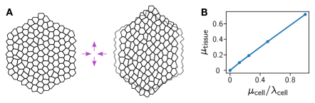
Figure S10: Cell-level shear modulus determines tissue level shear modulus. A Large-scale tissue shear are the lowest energy isogonal modes. Reference configuration (minimum energy for a given tension triangulation, left) and deformed configuration (right, outline shows reference configuration), deformed according to the isogonal Hessian eigenvector of one of the two lowest eigenvalues in an example tissue patch. B Tissue level shear modulus is proportional to cell level shear modulus. Tissue level isogonal shear modulus vs cell-level shear modulus for the tissue patch shown in A.

IV Model details and simulation methods

In the following, we explain the simulations presented in the paper and provide the modeling and implementation details. These comprise the mean-field calculation of the dynamics of the distribution of vertex angles, the symmetric lattice of a single intercalating quartet (shown in the companion paper [17]), and the tissue-scale simulation of a disordered epithelial tissue comprising both active and passive regions. All code used to create and analyse the simulations is available on GitHub https://github.com/nikolas-claussen/CE_simulation_public.

IV.1 Positive feedback tension dynamics and single-vertex simulation

We begin by describing the intrinsic tension dynamics of a single tension triangle. This is the basis for the singe-triangle simulation in Fig. 5, where we show the dynamics of the distribution of vertex angles predicted by a positive tension feedback model. Under this model, the edge tensions $\tilde{T}_{\alpha}$, $\alpha=1{-}3$, at a vertex evolve according to:

$$\tau_{\mathrm{T}}\dot{\tilde{T}}_{\alpha}=T_{\alpha}^{n}-\frac{1}{3}\sum_{\beta}\tilde{T}_{\beta}^{n}$$

where $n>1$ and $\tau_{\mathrm{T}}$ is a time scale converting simulation time into minutes. Note that we fix the overall tension scale by the constraint that the triangle perimeter $P=\sum_{\alpha}\tilde{T}_{\alpha}$ is fixed (corresponding to a finite total myosin pool). This simplified the analysis of saturating positive feedback below, and is consistent with the single-quartet simulations in the companion paper. Fixing the triangle area $A$ instead does not significantly affect the results for the single triangle simulations. The feedback exponent was taken as $n=4$ as in Ref. [17]. Different values give very similar results, so no systematic optimization was performed. We note that since the tension constraint $P=\mathrm{const.}$ or $A=\mathrm{const.}$ only affects the overall triangle size, and the trajectories in LTC space (but not their speed) are independent of it.

We integrated the tension dynamics using a 4th order Runge-Kutta method as implemented in the SciPy software package [56], using as initial conditions the vertex angles in the experimental data at time $t=5\>\text{min}$ (the vertex angles from the data were temporally smoothed with a window of $2\>\text{min}$ to reduce noise). From our simulation, we computed the LTC parameter to compare the marginals with the experimental data.

Dynamics in the LTC space.

To find the trajectories in the LTC space, we integrated Eq. (5). A change of variables from side length to the LTC space yields the flow shown in Fig. 5A. To model the effect of intercalations, which remove highly obtuse tension triangles from the distribution, we stopped integration once the maximum relative tension increased over $T_{\mathrm{rel}}=1.56$, the median of the relative tension at the moment of a T1 pbserved the tissue-scale simulations with isogonal stretching (as well as in the experimental data). These “collapse” triangles were removed from the simulation ensemble.

Fit of the tension timescale to experimental data.

To determine the tension timescale $\tau_{T}$, we compute the dynamics of the relative tension (the ratio of the edge tension to that of the adjacent edges) for all edges that undergo a T1 transition and align them temporally based on the time the T1 process occurs. This leads an average $T_{\mathrm{rel}}(t)$ that can be compared to the time traces from the experimental data reported in the companion paper[17] to fit $\tau_{T}$. Because the tension dynamics in the tissue-scale simulations is affected by tension balancing (see below), while the single-triangle and single-quartet simulations are not, we fit $\tau_{T}$ separately for the two classes of simulations. Note that we fit the tension timescale to a microscopic process, the T1 transition, and the resulting time course for macroscopic observables (tissue extension, LTC distribution) matches the experimental data without additional adjustment.

IV.2 Tension dynamics post intercalation: Myosin handover and passive tension

In the single-triangle simulations, we only consider dynamics up to the moment of intercalation. At this point, the tension triangulation is modified topologically: the edge corresponding to the collapsed interfaces is replaced by one corresponding to the new interface (triangulation “flip”). To complete our model, we must specify the initial conditions of this new edge.

As explained in the companion paper, we propose a myosin handover mechanism to explain the extension of the new interface post intercalation. A interface with cortical tension $T$ is comprised of the adherens-junctional actomyosin cortex of the two adjacent cells, which are coupled mechanically via adherens junctions. Under force balance, the total tension $T$ has to be constant along the cortex, but the individual tensions on either side can be non-uniform, as the resulting traction forces are exchanged via adherens junctions. In the following, we assume as a first order approximation that the level of active tension (i.e. myosin concentration) varies linearly along an interface (similar calculations have been performed in Ref. [57] to calculate interfacial shear stress). This allows us to geometrically obtain the myosin concentration at the individual cortices that will form the two juxtaposed sides of the new interface (see companion paper).

Consider a vertex, where interfaces $i=0,1,2$ (with tensions $T_{0},T_{1},T_{2}$) meet, and let $0$ be the interface about to collapse. For an illustration, see Ref. [17], Fig. 4). The three cells that meet at the vertex will be referred to by $(01),(12),(21)$ (where e.g. $(01)$ is the cell abutting interfaces $0$ and $1$). Let $m_{01},m_{12},m_{21}$ be the motor molecule concentrations (in units of tension) at the vertex in the junctional cortices of the three cells. Then, the tensions are related to the motor molecule concentrations as:

$$T_{0}=m_{21}+m_{01},\quad T_{1}=m_{01}+m_{12},\quad T_{2}=m_{12}+m_{21}.$$

This uses the assumption of myosin continuity at vertices, and the fact that the tension on an interface is the sum of the tensions of the two cortices that make it up. The motor molecule concentration on the cortex belonging to the new interfaces, post collapse, will be equal to $m_{12}$. Solving for this in terms of the tensions:

$$m_{12}=\frac{T_{1}+T_{2}-T_{0}}{2}$$

The new interface consists of two cortices, coming from the two vertices of the collapsed interface. Let the tensions at the two triangles be $T_{0},T_{1},T_{2}$ and $T_{0},T_{1}^{\prime},T_{2}^{\prime}$. Let $T_{a}$ be the active tension on the new interface immediately after the T1. It is the equal to

$$T_{a} =\frac{(T_{1}+T_{2}-T_{0})+(T_{1}^{\prime}+T_{2}^{\prime}-T_{0})}{2}$$ (30)

Note however that the total tension $T_{n}$ on the new interface is not necessary equal to $T_{a}$. The total tension is defined geometrically from the angles at the new interface (or, equivalently, the tension triangulation vertices). Indeed, generally, $T_{n}>T_{a}$, i.e. the active tension on the new interface is not enough to balance the tension due to the adjacent edges. As explained in the companion paper, we introduce a passive tension $T_{p}$ on the new edge which balances this deficit

$$T_{p}=T_{n}-T_{a}=T_{n}-(m_{12}+m_{12}^{\prime})$$

For example, if a perfectly symmetric quartet collapses when the vertex angle facing the collapsing edge is $90^{\circ}$, $T_{1}=T_{2}=T_{1}^{\prime}=T_{2}^{\prime}=1$ and $T_{0}=T_{n}=\sqrt{2}$. Therefore, $T_{a,n}=2-\sqrt{2}\approx 0.6$ and $T_{p,n}=\sqrt{2}-(2-\sqrt{2})\approx 0.8$. Note that by the triangle inequality, for any convex quadrilateral with perimeter $P$ and diagonals $D_{1},D_{2}$, one has $P/2\leq D_{1}+D_{2}\leq P$. Applying this to the quadrilateral formed by the two tension triangles at the collapsing interface, we get $T_{a,n}\geq 0$ and $T_{p,n}\geq 0$: the handover formula always results in positive active and passive tensions. Further, the “handover” mechanism robustly generates irreversible T1s: if a interface were to collapse back after a T1, the newly formed interface would inherit high myosin levels and therefore be likely to collapse again.

The passive tension subsequently relaxes visco-elastically with rate $\tau_{p}^{-1}$: $\dot{T_{p}}=-\tau_{p}^{-1}T_{p}$. Combining this with the feedback equation, the evolution of the total tension is

$$\dot{\tilde{T}}=\tau_{T}^{-1}\left(T^{n}-\frac{1}{3}\sum_{\beta}\tilde{T}_{\beta}^{n}\right)-\tau_{p}^{-1}T_{p}$$ (31)

where we assumed that the positive feedback only operates on the active tension. The relaxation time scale was chosen at $\tau_{p}=\tau_{T}/4$, which fits the observed decay of tension post T1. If the tension relaxation rate $\tau_{p}^{-1}$ is too low, then positive tension feedback leads to a reversal of active T1s, and the T1 gets stuck at the 4-fold vertex configuration.

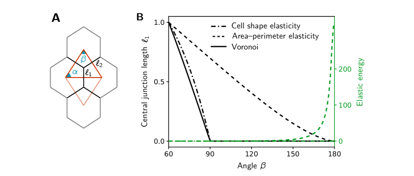
Figure S11: Absence of energy barrier to intercalations A Length of the central interface in a quartet for a prescribed isosceles tension triangle parametrized by the angle $\beta$ (the isosceles property implies $\alpha=(\pi-\beta)/2$). B The solid line shows the interface length in the Voronoi tessellation $\ell_{\mathrm{ref}}$ (cf. Eq. (10)). The interface length obtained by minimizing elastic energy Eq. (3) with isotropic target shape (dot-dashed line) closely follows the Voronoi length and vanishes at the same critical angle. By contrast, minimizing the “area–perimeter” energy of the vertex-model $E_{\mathrm{cell}}\sim(A-A_{0})^{2}+(P-P_{0})^{2}$ gives a interface length (dashed black line) that vanishes only for $\beta\to\pi$ and the energy diverges in this limit (dashed green line).

IV.3 Cell shape elasticity

As explained in the main text, in our model, tension dynamics translate into tissue dynamics via force balance which we implement by minimizing the energy function Eq. (1). Here, we explain our choice of the term representing cell-shape elasticity, $E_{C}$. We use an elastic energy based on the the cell shape tensor

$$S_{\mathcal{C}}=\sum_{i}\frac{\mathbf{e}_{i}\otimes\mathbf{e}_{i}}{|\mathbf{e}_{i}|}$$

where $i$ runs over the edges of the cell $\mathcal{C}$, and $\mathbf{e}_{i}$ is the vector pointing from one vertex of the interface to the other. Note that in this shape tensor, each edge contributes linearly in length to the cell shape. This means that artificially subdividing an edge has no effect on the cell shape tensor. This makes sense if we assume that the elasticity we aim to model using $S$ resides in the cell interior (incompressibility, microtubules, intermediate filaments, nucleus). The shape tensor can also be defined using vectors from the cell centroid to its vertices (in the lattice, the two definitions are equivalent). An alternative definition of the elastic energy using $\tilde{S}_{\mathcal{C}}=\sum_{i}\mathbf{e}_{i}\otimes\mathbf{e}_{i}$ instead gives broadly similar results (although interface collapse happens more abruptly, because of the higher order non-linearity).

We assign a reference shape $S_{0}$ and define the cell elastic energy via

$$E_{\mathcal{C}}=\lambda[\mathrm{Tr}(S_{\mathcal{C}}-S_{0})]^{2}+\mu\mathrm{Tr}[(S_{\mathcal{C}}-S_{0})^{2}]$$ (32)

with bulk modulus $\lambda$ and shear modulus $\mu$. The reference shape $S_{0}$ controls the isogonal mode. An isotropic $S_{0}\propto\mathrm{Id}$ favours equilateral hexagons. We used a shear/bulk ration of $\mu/\lambda=1$ for all “active” cells in the simulations. Because of the separation of scales between cortical tensions and elastic energy baked into the model, the absolute values of $\lambda,\mu$ are irrelevant.

Strikingly, when the cell array is a symmetric lattice (single-quartet simulations shown in the companion paper), the “shape strain” $S_{\mathcal{C}}-S_{0}$ can always be set to 0 by choice of the edge lengths, and the energy $E_{\mathcal{C}}=0$ throughout. This can already be seen from a degree-of-freedom count (three $\ell_{i}$ for the three independent components of $S_{\mathcal{C}}-S_{0}$). The elastic energy therefore acts only on the isogonal modes (i.e. $\partial_{\phi_{i}}E_{\mathcal{C}}|_{\ell_{i}=\mathrm{minimizers}}=0$) and there is no energy barrier for intercalations. Consequently, there is no need for noise to drive intercalations in our model. By contrast, for the widely-used area-perimeter elastic energy $E=(A-A_{0})^{2}+(P-P_{0})^{2}$ (where $A,P$ are the cell area and perimeter, and $A_{0},P_{0}$ their target values) [24], there exists an energy barrier, and the inner interface $\ell_{0}$ only collapses when $\phi_{0}=\pi$. This is shown in Fig. S11B. Note that the area-perimeter energy is a special case because of the geometric incompatibility of area and perimeter constraints. Combining area elasticity with shear elasticity based on the shape tensor, $E=(A-A_{0})^{2}+\mu\mathrm{Tr}[(S_{\mathcal{C}}-S_{0})^{2}]$, (or perimeter elasticity with cell shape bulk elasticity) leads to similar results as Eq. (3). Note also that because of the degree-of-freedom count, the system is under-specified if the shear modulus is 0, foreshadowing the fact that without shear modulus, no convergence-extension takes place.

IV.4 Tissue scale simulation

Using the components of the single-quartet simulation, we now describe a simulation of an arbitrary, disordered tissue patch. The key assumption are again adiabatic force balance and cortical tension dominance: the tissue geometry is found by solving for force balance, by first finding the angles from the cortical tensions and then the isogonal mode by minimizing cell elastic energy. The key quantity is the tension triangulation whose dynamics determines the tissue dynamics.

Conceptually, there is one main novel element: since the tension triangulation is now disordered and comprises many heterogeneous tension triangles, an additional mechanism is required to ensure the tension triangles fit together to a global triangulation. Further, the higher computational load requires different numerical methods.

Data structure.

We model a piece of epithelial tissue by a polygonal tiling of the plane, polygons corresponding to cells. Two cells are neighbors if they are share an edge (this implies that the cell adjacency graph is a triangulation).

Following the idea of the dual tension triangulation introduced in the main text, a polygonal tiling is represented by a triangular mesh, in which cells are represented by vertices, cell edges by triangulation edges, and cell vertices by triangulation faces. Vertices, edges, and faces have the following attributes which are used for time evolution:

• Vertices: dual coordinates, the $x,y$ coordinates of the vertex in the tension triangulation which will be denoted $\mathbf{t}_{i}$, and the reference shape $g_{0}$ for the shape-tensor elastic energy.

• Edges: the active and passive tensions on an edge.

• Faces: primal coordinates, the $x,y$ coordinates of the vertex in the cell tessellation corresponding to the face, denoted $\mathbf{r}_{ijk}$.

Given the dual coordinates of two adjacent vertices $\mathbf{t}_{i},\mathbf{t}_{j}$, the tension on the edge connecting cells $i,j$ is $T_{ij}=|\mathbf{t}_{i}-\mathbf{t}_{j}|$. The dual coordinates encode a configuration of balanced cortical tensions. Note that the primal (cell) and dual (tension) coordinates live in different spaces, and the overall scale of the tension coordinates is irrelevant.

The mesh is implemented in object oriented python, using a half-edge mesh data structure [58]. A half-edge mesh consists of vertices, faces, and, for each edge, two oriented half-edges. A half-edges stores a reference to the next half-edge on the counter-clockwise oriented face it belongs to, and a reference to its twin, the half-edge with opposite orientation on the adjacent face. This structure defines an orientation for every triangular face and makes mesh traversal (e.g. get all vertices of a cell) and mesh modification (e.g. intercalations) very convenient.

Overview.

Due to the assumption of adiabatic force balance, the tissue geometry is determined by the instantaneous tensions. The dynamics is therefore determined by the change in the tension triangulation (due to positive feedback). In detail, the time evolution in our simulation is done in three steps:

1. Local Euler step: For each triangular face, update the active tensions according to positive tension feedback, and the passive tensions and the rest shape according to viscous relaxation.

2. Triangulation flattening: Optimize the dual vertex positions so that the lengths of each half-edge is as close as possible to its internally stored tension. This ensures global tension balance.

3. Cell shape optimization: Optimize the primal vertex positions to minimize the shape-tensor based elastic energy, while constraining the angles by the dual triangulation.

4. Topological modifications: Check if any primal edge has collapsed and carry out intercalations if necessary, re-initializing the active and passive tensions on the new edge.

The next sections describe them in detail. The most complicated and time-consuming of them is the cell shape optimization. Overall, a simulation of convergent extension of $\sim 1000$ cells takes approx. 15 minutes on a current-generation laptop.

Triangulation dynamics.

For each mesh half-edge, we store the total intrinsic and passive tensions $\tilde{T}_{aij},T_{p,ij}$. We collect the total and passive tensions from all half-edges $ij$ belonging to a triangular face $I_{ijk}=\{(ij),(jk),(ki)\}$ and carry out an explicit Euler step with step size $\sim 10^{-3}$ according to the following dynamics:

$$\tau_{T}\partial_{t}\tilde{T}_{ij} =\tilde{T}_{ij}^{n}-k_{\text{cutoff}}\tilde{T}_{ij}^{n+1}-\frac{1}{3}\sum_{\alpha\in I_{ijk}}(\tilde{T}_{\alpha}^{n}-k_{\text{cutoff}}\tilde{T}_{\alpha}^{n+1})-\frac{\tau_{T}}{\tau_{p}}T_{p,ij}$$ (33)

$$\tau_{p}\partial_{t}T_{p,ij} =-T_{p,ij}$$ (34)

The cutoff parameter $k_{\text{cutoff}}$ stops runaway positive feedback at values $T>1/k_{\text{cutoff}}$. It is not strictly necessary since runaway feedback is cut short by intercalations, but helpful for long-time simulations, were rarely, run-away tension cable configurations can occur which can blow up numerically. We chose $1/k_{\text{cutoff}}=5\bar{T}$ where $\bar{T}$ is the overall tension scale, so that it has almost no effect in normal tension configurations. We chose the feedback parameter $n=4$ and the relaxation rate $\tau_{p}=\tau_{T}/4$, the same used in the single-quartet and single-triangle simulations.

So far, the time evolution of tensions is purely autonomous (i.e. each tension triangle is independent from all others) and completely analogous to the single-quartet simulation. In the single-quartet simulation, all tension triangles are equal by symmetry and periodicity, and thus tile the plane as a triangulation by construction. In general, this is no longer guaranteed. Even if one starts with a flat tension triangulation, the autonomous time evolution Eq. (34) will result in a set of tension triangles that cannot fit together to a flat triangulation. The triangulation will develop curvature [12], i.e. “crumple” out of plane. This means that we have to add an additional ingredient to enforce triangulation planarity.

In principle, the constraints enforcing planarity (one constraint per triangulation vertex) can be worked out explicitly [13]. In practice, we enforce this projection as follows. The set of all balanced tension triangulations is parameterized by the dual vertex positions $\mathbf{t}_{i}$. We therefore seek the balanced tension configuration that approximates the intrinsic tensions as closely as possible by minimizing the following elastic energy:

$$E_{\text{tri}}=\frac{1}{2N_{\text{edges}}}\sum_{ij}(||\mathbf{t}_{i}-\mathbf{t}_{j}||-\tilde{T}_{ij})^{2}+\frac{1}{2N_{\text{triangles}}}\sum_{ijk}\mathrm{Pen}(A_{ijk},A_{0})$$ (35)

Since the simulation is based on half-edges, the per-edge intrinsic tension $\tilde{T}_{ij}$ is the average of the tensions of the two half-edges (which can be though of as the two cellular cortices coupled in a cell-cell interface).

The second term, $\mathrm{Pen}(A,A_{0})$ is a penalty term on the triangle areas $A$ (calculated from the vertex positions $\mathbf{t}_{i}$). It fixes the overall tension scale (which is arbitrary due to force balance) and ensures the triangulation is well behaved numerically. It contains two terms:

$$\mathrm{Pen}(A,A_{0})=\gamma_{\text{tri}}\left(100\cdot(\max\{0,\frac{A_{0}}{4}-A\})^{2}+\frac{1}{2}(A-A_{0})^{2}\right)$$ (36)

Here, $A_{0}$ is an arbitrary reference area fixing the overall tension scale. Because the triangular mesh is oriented, the area $A_{ijk}$ is signed, with negative signs corresponding to un-physical “flipped” configurations. These, and degenerate triangles, are penalized by the first term. The second term is a soft potential fixing the overall tension scale and preventing isotropic growth. The penalty strength $\gamma$ was chosen at $10^{-3}$, so that the area penalty represents a small correction to the length-term.

In the simulation, we first carry out an explicit Euler step for the intrinsic tensions, and then “flatten the triangulation”, i.e. find the dual vertex positions by minimizing Eq. (35). This determines the extrinsic tensions $T_{ij}=||\mathbf{t}_{i}-\mathbf{t}_{j}||$. Finally, we relax the intrinsic tensions to force balance with rate $\tau_{\mathrm{balance}}$,

$$\frac{d\tilde{T}_{ij}}{dt}=-\tau_{\mathrm{balance}}^{-1}(\tilde{T}_{ij}-T_{ij})$$ (37)

In order to ensure numerical stability even for large $\tau_{T}$, we use the exact solution of Eq. (37) numerically, instead of carrying out an explicit Euler step.

The triangulation-flattening prescription can be thought of as modelling, indirectly, known feedback loops which lead to a convergence to balanced tension, most importantly, strain-rate feedback [13], which has been demonstrated experimentally [14]. The rate $\tau_{\mathrm{balance}}^{-1}$ determines the speed of these feedback loops.

Directly modelling of this effect requires going beyond the separation between tension- and real-space-dynamics that is the basis of our model here and is therefore beyond the scope of this paper. Further, the triangulation-flattening prescription is the most parsimonious generalization of the local tension feedback dynamics employed in the single-quartet simulation to a disordered tissue patch.

The complete tension dynamics that is implemented in the simulation therefore comprises three terms in addition to the dynamics shown in the main text Eq. (5): (1) Numerical cutoff of positive feedback at very high tensions (2) Passive tension dynamics post T1 (3) Relaxation of tensions to force equilibrium:

$$\partial_{t}\tilde{T}_{ij}= \tau_{\mathrm{T}}^{-1}\left(\tilde{T}_{ij}^{n}-k_{\text{cutoff}}\tilde{T}_{ij}^{n+1}-\frac{1}{3}\sum_{\alpha\in I_{ijk}}(\tilde{T}_{\alpha}^{n}-k_{\text{cutoff}}\tilde{T}_{\alpha}^{n+1})\right)$$ (38)

$$-\tau_{p}^{-1}T_{p,ij}-\tau_{\mathrm{balance}}^{-1}(\tilde{T}_{ij}-T_{ij})$$ (39)

We find that our simulations are robust to different choices of the tension dynamics parameters $\tau_{p},\tau_{\mathrm{balance}},k_{\mathrm{cutoff}}$, as demonstrated in Fig. S7. We can, for instance, decrease the balancing time by $40\times$ without affecting the qualitative behavior.

Cell shape dynamics.

Above, we have described the dynamics of the tension triangulation. After an Euler step to update the tensions has been taken, we calculate the real space cell tessellation (i.e. the positions of the cell vertices) by minimizing the cell-shape elastic energy while constraining the angles by the tension triangulation. In the case of a single quartet of identical cells, we could explicitly parameterize the cell shape by interface lengths and angles, and optimize only with respect to the former. In the disordered case, it is more convenient to enforce the angle constraint via a (strong) energy penalty. It would also possible to instead directly optimize the per-cell isogonal potentials $\Theta_{i}$ with respect to the Voronoi reference, obviating the need for a penalty.

The elastic energy to minimize therefore has two terms – the cell elastic energy Eq. (3) calculated from cell shape tensor $S_{\mathcal{C}}$ Eq. (IV.3) and reference shape $S_{0}$, and the angle penalty, which corresponds to the cortical tension energy term:

$$E=\frac{1}{2N_{\text{edges}}}\sum_{ij}T_{ij}(1-\hat{n}_{ij}\cdot\hat{\mathbf{r}}_{ij})+\frac{\epsilon}{N_{\text{cells}}}\sum_{i}E_{\mathcal{C},i}$$ (40)

Here, $\hat{n}_{ij}$ is the the unit normal of the tension edge, and $\hat{\mathbf{r}}_{ij}$ the unit tangent vector of the primal edge. The small parameter $\epsilon$ (we use $\epsilon\sim 10^{-3}\lambda^{-1}$) represents the fact that the cell shape energy is assumed to be much weaker than the cortical tensions. If desired, one can replace or modify the cell shape elastic energy $E_{\mathcal{C}}$ in Eq. (40) by another energy, e.g. the common area-perimeter elasticity.

In Eq. (40), we use a different term than the standard $\sum_{ij}T_{ij}\ell_{ij}$ to represent the cortical tensions. The reason for this is numerical: Eq. (40) is well-behaved for short edges, does not require a pressure-term to prevent collapse of the cell array, and ensures only “valid”, self-intersection-free mesh configurations are energy minima. It is however equivalent to the standard form $\sum_{ij}T_{ij}\ell_{ij}$ near force balance (i.e. the energy minima): both terms enforce the angle constraints implied by the tensions $T_{ij}$ in force balance. The angle penalty enforces that the angle between the dual tension edge and the real-space edge is $90^{\circ}$ by using the unit normal $\hat{n}_{ij}$ of the tension edge, and the unit tangent vector $\hat{\mathbf{r}}_{ij}$ of the primal edge. We can also rewrite this as follows:

$$T_{ij}(1-\hat{n}_{ij}\cdot\hat{\mathbf{r}}_{ij})=\frac{T_{ij}}{2}||\hat{\mathbf{r}}_{ij}-\hat{n}_{ij}||^{2}=\frac{1}{2}||\mathbf{T}_{ij}-R(\tfrac{\pi}{2})\mathbf{t}_{ij}||^{2}$$ (41)

where $\mathbf{T}_{ij}$ is the real-space tension vector, $R(\tfrac{\pi}{2})$ a $90^{\circ}$ rotation matrix, and $\mathbf{t}_{ij}=\mathbf{t}_{i}-\mathbf{t}_{j}$ the dual tension vector, defined by the tension vertices.

To understand the particular form $\hat{n}_{ij}\cdot\hat{\mathbf{r}}_{ij}$, recall that every triangulation edge $\mathbf{t}_{i},\mathbf{t}_{j}$ is represented twice, as two oriented half-edges belonging to the two faces which meet at the edge. Using this orientation, for a half-edge edge $i\rightarrow j$, we can compute the dual outward facing unit normal $\hat{n}_{ij}$. We then compare $\hat{n}_{ij}$ to the primal edge unit vector $\hat{\mathbf{r}}_{ij}=\hat{\mathbf{r}}_{(ij)(ji)}$ from the primal vertex of the triangle $(ij)$ belonging to $i\rightarrow j$ to that of the apposing triangle $(ji)$. The angle penalty ensures firstly, that the primal edges are orthogonal to the correspondingly dual edge, implementing the tension constraint on angles. Secondly, it automatically penalizes “invalid” vertex positions, e.g. “bowties” in which a primal vertex of one cell lies within the neighboring cell. Such situations correspond to $\hat{\mathbf{r}}_{(ij)(ji)}$ anti-parallel to $\hat{n}_{ij}$, which is why we chose a slightly elaborate form for the angle penalty.

After carrying out a local Euler step and updating the dual vertex positions by “triangulation flattening”, we find the primal vertex positions by minimizing the elastic energy Eq. (40).

Topological modifications.

After each time-step we check whether any edge has collapsed. We call an edge collapsed if its length is $<10\%$ of the overall length scale (mean edge length at simulation start). If this occurs, we carry out an intercalation (flip the corresponding edge in the triangulation) and set the active and passive tensions on the new edge as described above.

Edges that underwent a T1 transition in the last 20 simulation time steps (corresponding to 2.5 minutes) are excluded from edge collapse so as to prevent the immediate re–collapse of newly formed junctions. Instead of this hard-coded criterion, one could also calculate the strain rate of junctions of short length and exclude extending junctions, as shown by the time traces of junction length in Fig. 8B.

Automatic differentiation and numerical optimization.

The simulation requires solving two optimization problems, one for the triangulation Eq. (35) and one for the real-space shape Eq. (40). To solve an optimization problem efficiently, it is crucial to know the gradient of the objective function. We use the python library JAX [59] to automatically differentiate our energy functions, allowing easy, rapid and bug-free calculation of the Jacobians. We further use JAX’s just-in-time functionality to accelerate our python code. Gradient-based optimization requires the objective function to be at least once differentiable. To ensure this, we mollify functions as required; for example, the Euclidean norm $\sqrt{x^{2}+y^{2}}\rightarrow\sqrt{x^{2}+y^{2}+\epsilon^{2}},\>\epsilon\sim 10^{-3}$ to ensure differentiability when computing the lengths of very short edges.

With these tools, the energies can be efficiently minimized using scipy’s conjugate-gradient optimizer. With a relative tolerance of $10^{-5}$, a shape optimization step for $\sim 1000$ cells takes $\sim 10\text{s}$ on a laptop. Using the half-edge data structure described above, and JAX-based automatic differentiation, we can also easily construct the isogonal Hessian $\mathcal{H}_{ij}$ analyzed in Fig. S10.

Creation of initial conditions.

Finally, we need to specify the simulation the initial conditions. Note that because the cell vertex positions are computed from the tension triangulation, in our initial condition we specify only the tension triangulation.

We consider two types of initial conditions, using either a regular lattice or a random point process to choose the tension vertices. In the former case, we chose rectangular patches of a regular triangular lattice, with i.i.d. Gaussian noise added to the vertex positions. The amplitude of the noise was chosen so that $\mathrm{std}(T_{ij})=0.15\>\mathrm{mean}(T_{ij})$. The influence of the Gaussian noise standard deviation is shown in Fig. S7. A triangular lattice corresponds to a hexagonal lattice of cells. Indeed, locally, the Drosophila embryo at the onset of GBE looks like it is composed out of (noisy) hexagonal lattice patches, as shown in Fig. S1. This lattice is subjected to a small initial strain to create an a initial tension anisotropy, as described in the main text.

To investigate the effect of disorder, we also create initial conditions using a hard disk process. This randomly samples 2d-points (the eventual vertices in tension space) under the constraint that no two points are closer than $2r$ where $r$ is the “hard disk” radius. Instead of $r$, we use the normalized hard disk packing fraction $\rho\in[0,1]$, which is maximal for a hexagonal lattice. At $\rho\sim 0.72$, the hard disk process undergoes a phase transition that destroys the lattice order. The limit $\rho=0$ corresponds to a Poisson point process. To sample from a hard disk point process, we use the event-chain Monte Carlo algorithm of Ref. [25], with code based on that provided with Ref. [26]. Note that with other algorithms such as sequential deposition or standard Monte Carlo it is either impossible or prohibitively slow to sample at arbitrary values of $\rho$.

To create a tension triangulation, we then compute the Delaunay triangulation of this point set (we further refine the initial condition by removing the edge of this tension triangulation, where the Delaunay algorithm can create very long tension edges). This triangulation is stretched uniformly to set up the initial anisotropy of tension. Cell numbers and initial aspect ratios were also chosen identically in the simulations that make up the phase diagram of Fig. 3.

Boundary conditions, tissue patterning, and isogonal stretching.

For the first half of the work, Figs. 2-5, we use a tissue made of identical cells with free boundary conditions. We now specify the boundary conditions, and the division of the tissue into active and passive patches of the simulations for Figs 7-8.

We use appropriate boundary conditions to mimic the geometry of the Drosophila lateral ectoderm. We consider a initially rectangular tissue patch with height $>$ width. The top/bottom edges correspond to the dorsal pole, the middle to the ventral region, and the left/right sides to the anterior/posterior edges of the lateral ectoderm. To simulate the cylindrical geometry of the Drosophila trunk, the top/bottom boundary are given slip-wall boundary conditions, i.e. the cells on the boundary are pinned along the $y$-axis and free to move along the $x$-axis. The left/right boundaries are free. Boundary conditions are numerically implemented by a confining potential which penalizes deviation of the $x$ or $y$ coordinate of the cell centroids designated to be boundary cells from the location of the slip wall. This allows for flexible implementation of various boundaries and geometries. We can also chose different boundary conditions. We can also add slip walls on the left/right boundaries to model the experiments carried out in Ref. [8], where GBE was blocked by cauterization of the ventral tissue close to the posterior pole.

Next, we designate active and passive regions in the tissue. In the active region, tensions evolve in time according to excitable tension feedback Eq. (34). In the passive regions, tensions are governed by homeostasis (see below), and cells are softer. To simulate a wild type embryo, we chose the size of the passive patch to be approximately 40% of the embryo circumference (the exact value does not have an important influence). To mimic an embryo without modulation of activity along the DV axis (e.g. a TollRM9 mutant), all cells along the embryo were taken to be active. The cells at the very tissue boundary are always passive for reasons of numerical stability. Otherwise edges on the boundary could undergo a T1, which leads to an invalid state.

We can take model a situation where the cells in simulated tissue are initially stretched isogonally. This can be encoded by stretching the tissue using the slip wall boundary conditions; instead, we set the cell reference shape $S_{0}$ to an anisotropic matrix, as discussed above in the SI. For the simulations of the Fig. 7 and 7, we set the initial stretching to 0.

Dynamics of tensions and cell shapes in passive cells.

To model the cells in passive tissue regions in our simulations, we must prescribe their tension dynamics and their cell elasticity. Regarding the tension dynamics, we assume that it is governed by tension homeostasis. This means that the intrinsic tensions $\tilde{T}_{ij}$ in the passive region behave as:

$$\frac{d\tilde{T}_{ij}}{dt}=-\tau_{h}^{-1}(\tilde{T}_{ij}-\tilde{T}_{ij,0})$$ (42)

where $\tau_{h}$ is the homeostasis timescale, and $\tilde{T}_{ij,0}$ is the tension on the edge at the beginning of the simulation. For newly generated edges after a passive T1, we generate a random reference value $\tilde{T}_{ij,0}\approx 1$. One can also set $\tilde{T}_{ij,0}\equiv 1$ for all passive cells, in which case the passive tissue relaxes to a hexagonal lattice. The speed of homeostasis $\tau_{h}$ has no strong influence on the simulations, but must be large enough so that tensions relax after a passive T1 process, before a second passive T1 process takes place. In our simulations, we always set $\tau_{h}=\tau_{p}$, the speed of passive tension relaxation in the active tissue.

Regarding cell shape dynamics, we model the passive tissue as very soft. In particular, we assume that their shear modulus is very low: $\mu_{p}=0.2\mu_{a},\;\lambda_{p}=0.2\lambda_{a}$ where the subscripts _a and _b refer to active and passive cells, respectively. Further, we use a lower value of the angle-constraint penalty $1/\epsilon$ than in the active region: $1/\epsilon_{p}=1/(200\epsilon_{a})=5$. This accounts for the fact that in the passive region, the elastic moduli are much lower (so $1/\epsilon_{p}$ must be decreased to keep the ratio constant), as well as for the fact that in the passive region, we expect weaker tension. Tension is still the dominant force and the cell array angles match the angles prescribed by the triangulation to within $\sim 2^{\circ}$. However, we find that small deviations from the triangulation are important to facilitate passive T1s.

Simulation statistics and computing resources

For each measurement show in the figures of this paper, by default, we pooled or averaged 3 simulation runs with identical parameters, but different random seeds for the creation of the initial tension triangulation. The phase diagram Fig. 3A shows the average of 6 simulation runs each. The trajectories in Fig. 7 as well as the interface length and orientation statistics in Fig. 8 were computed from a single simulation.

By default, simulated meshes had $N_{\mathrm{cells}}\approx 10^{3}$ cells (the exact number could vary slightly due to randomness in the hard disk point process). Simulations of saturating feedback in Fig. 5 had $N_{\mathrm{cells}}\approx 350$ cells, and simulations in Figs. 7-8 had $N_{\mathrm{cells}}\approx 750$ cells. Simulation edges were always excluded from analysis. For the single–triangle simulation in Fig. 5, we simulated $4\times 10^{3}$ individual triangles from the initial condition of the full numerical simulations. When showing time traces, we smoothed the T1-rate and aspect ratio time series with a Gaussian kernel of width $10dt$ where $dt=\tau_{T}/200$ is the simulation time step. Numerical parameters were adjusted so that elastic energy minimization and triangulation flattening converged for all simulations and all time points.

Simulations were carried out on a Supermicro workstation with 64 Intel Xeon Gold 6326 cores and 256GB of RAM. However, individual simulations (rather than parameter scans and phase diagrams) can be run without problem on a consumer grade laptop.

Overview of model parameters and their effects.

As a summary, Table 1 gives a list of all the parameters of the tissue-scale model displayed in this work, as well as their default values. Fig. S7 shows analyses of simulations where several of the parameters are varied, confirming that the qualitative behavior of the model is largely independent of the exact parameter values.

Model parameters	symbol	default value	effect
Tension time scale	$\tau_{T}$	$25\;\mathrm{min}$	Fitted to experimental T1 tension dynamics.
Feedback exponent	$n$	$4$	Must be $>0$ to produce flow. Weak effect on TCE.
Tension balancing	$\tau_{\mathrm{balance}}$	$\tau_{T}/200$	Must be $\ll\tau_{T}$. Higher values lead to a higher rate of disoriented T1s.
Passive tension relaxation	$\tau_{p}$	$\tau_{T}/6$	No strong effect. Must be sufficiently small $<\tau_{T}/2$ to create irreversible T1s.
Elasticity coefficient ratio	$\mu/\lambda$	$1$	No strong effect. Must be $>0$
Passive region shear moduli	$\mu_{\text{p}}/\mu_{a},\>\lambda_{p}/\lambda_{a}$	$0.2,\>0.2$	$\mu_{a}/\mu_{p}>1$ or passive tissue resistance lowers TCE.
Initial condition parameters
Initial anisotropy	$||\langle\sqrt{2}\tilde{Q}\rangle||$	$0.2$	Higher values increase TCE.
Tension vertex hard disk packing fraction	$\rho$	$0.45-0.9$	Higher values increase TCE.
Gaussian noise in initial tensions (standard deviation)		$0.1\>\overline{T}$	Weak effect on TCE, as long as noise is sufficiently weak to not affect triangulation topology.
Cell reference shape	$S_{0}$	$3\ell_{0}\>\mathbb{I}$	Anisotropic $S_{0}$ increases bridge bias by shifting T1 threshold.
Number of cells	$N_{\mathrm{cells}}$	$\approx 10^{3}$	Number can vary due to random sampling. “Germ band” simulations had $N_{\mathrm{cells}}=750$.
Numerical parameters
Tension feedback cutoff	$k_{\mathrm{cutoff}}$	$0.3\overline{T}$
Triangulation area penalty	$\gamma_{\text{tri}}$	$0.01$
Angle constraint penalty	$1/\epsilon$	$10^{3}$	In the passive region, we use $1/\epsilon=5$.
Boundary condition penalty		$5\times 10^{3}$
Time step	$dt$	$0.5\times 10^{-2}\>\tau_{T}$
Edge length to trigger collapse		$0.1\>\ell_{0}$

Table 1: Parameters of tissue scale simulation. A value in the second-to-last column indicates a “default” value which was used in all simulations except otherwise indicated. $\overline{T}$ is the overall tension scale (average edge tension at initial condition), and $\ell_{0}$ the overall length scale (average edge length at initial condition). We use the abbreviation “TCE” for total convergent extension, i.e. the amount of convergent extension as tissue flow saturates.

V Movie captions

Movie 1: Simulation of convergent extension for ordered and disordered initial cell arrays.

Simulation of tissue scale model of convergent extension with ordered (left) and disordered (right) initial conditions, corresponding to Fig. 2. The number of cells and the initial tension anisotropy, as well as all other parameters, are the same for both simulations. The simulations were carried out with free boundary conditions. Top row shows the cell arrays, colored by cell coordination number (hexagons=white), bottom row the underlying tension triangulation. If the initial cell array is disordered, both the tissue and the tension triangulation extend only very little.

Movie 2: Simulations comparing saturating and winner-takes-all tension feedback.

Comparison of saturating (left) and winner-takes-all (right) tension feedback Fig. 5. Both simulations were initialized identical initial conditions (an ordered cell array with 20% tension anisotropy). All other parameters are the same for both simulations. Top row shows the cell arrays, colored by cell coordination number (hexagons=white), bottom row the underlying tension triangulation. Saturating feedback leads to little large scale shape change and creates tension cables.

Movie 3: Simulation of convergent extension in embryo-like geometry.

Simulation of tissue scale model of convergent extension in an embryo-like geometry, corresponding to Fig. 7. The embryo is modeled by a rectangular tissue patch with slip walls on the top and bottom edge, mimicking the embryo’s cylindrical geometry. The active and passive tissue regions, indicated by color and shading of the edges (color/solid=active), correspond to the germ band and the amnioserosa, respectively. Left: Cell tessellation with black dots indicating the cells along the slip wall (restricted to move along horizontally along the “AP axis”). Right: underlying tension triangulation. The tension triangulation is initialized with the experimentally observed initial tension anisotropy which breaks rotational symmetry and aligns the tissue extension along the “AP axis”. Colored dots follow a selected subset cells to highlight rearrangements.

Movie 4: Simulation of convergent extension without cell rigidity and without DV modulation of activity.

Simulation of tissue scale model of convergent extension in an embryo-like geometry for a control and two “mutant” configurations, corresponding Fig. 8. Left: “Control”, as in Movie 3. Middle: Active tissue with vanishing shear modulus $\mu_{a}=0$. Right: No DV modulation, i.e. no soft, passive region. All other parameters are identical. Top shows cell array, bottom underlying tension triangulation. Active and passive tissue regions are indicated by color and shading of the edges (color/solid=active). In all three conditions, active T1s drive elongation of the tension triangulation, while the convergent extension of the cell array only occurs for the “control” condition.