Regularized Reduced Order Lippmann-Schwinger-Lanczos Method for Inverse Scattering Problems in the Frequency Domain
Abstract
Inverse scattering has a broad applicability in quantum mechanics, remote sensing, geophysical, and medical imaging. This paper presents a robust direct reduced order model (ROM) method for solving inverse scattering problems based on an efficient approximation of the resolvent operator regularizing the Lippmann-Schwinger-Lanczos (LSL) algorithm. We show that the efficiency of the method relies upon the weak dependence of the orthogonalized basis on the unknown potential in the Schrödinger equation by demonstrating that the Lanczos orthogonalization is equivalent to performing Gram-Schmidt on the ROM time snapshots. We then develop the LSL algorithm in the frequency domain with two levels of regularization. We show that the same procedure can be extended beyond the Schrödinger formulation to the Helmholtz equation, e.g., to imaging the conductivity using diffusive electromagnetic fields in conductive media with localized positive conductivity perturbations. Numerical experiments for Helmholtz and Schrödinger problems show that the proposed bi-level regularization scheme significantly improves the performance of the LSL algorithm, allowing for good reconstructions with noisy data and large data sets.
1 Introduction
The inverse scattering problem formulated for the Helmholtz and Schrödinger operators arises in various fields, including quantum mechanics, remote sensing, geophysical, and medical imaging. The goal of imaging is to find the potential or properties of the medium in the domain using near-field measured data. There are different approaches to the inverse problem, starting with an original method based on the solution of a set of integral equations developed in celebrated works of Gelfand & Levitan, Marchenko, and Krein. In different formulations appropriate for particular applications, the existence and uniqueness of the solution of inverse scattering problems, as well as computational approaches, were discussed in many now classical works. Efficient numerical methods for inverse scattering have been developed in application to acoustic imaging, electromagnetic sensing, and seismic exploration; among them are iterative methods for full-wave inversion based on the adjoint or backpropagation method, techniques based on Born and Rytov approximations, layer stripping methods, asymptotic methods specifically developed for small volume inhomogeneities, as well as Kirchhoff migration and solving the Lippmann-Schwinger (LS) integral equation, see for instance [44, 11, 23, 38, 12, 49, 13, 2, 21, 20, 47, 40, 25, 1] and references therein. Formulated as the identification of the parameters of a layered medium, inverse scattering is related to cascade realizations of the transfer functions for digital filters or the minimal realization problem, actively discussed in electrical engineering and control theory literature [35, 19, 45]. Following the terminology used in that field, we refer to the inverse problems as single-input single-output (SISO) and multiple-input multiple-output (MIMO), depending on the problem setting.
The present work develops a robust direct reduced-order model method for solving inverse scattering problems for the Schrödinger and Helmholtz equations based on a Lippmann-Schwinger-Lanczos (LSL) algorithm in the frequency domain with two levels of regularization. This is the third paper in a series on the reduced order model (ROM) Lippmann-Schwinger-Lanczos (LSL) algorithm [29],[30]. Here, we advance the algorithm foundation, develop a robust regularization scheme, and extend the area of applicability of the method. Presented numerical experiments demonstrate that the regularized LSL method results in accurate reconstructions with noisy data and large data sets.
Our approach is based on the approximation of a resolvent operator and constructing a Reduced Order Model (ROM) that allows effectively substitute solving a large-scale inverse problem with a problem of much smaller size. Such a reduction of the size of the numerical problem has irrefutable advantages in saving computational time and required storage memory. ROMs are generally constructed by projecting the solution of a large-scale problem into an appropriate subspace [4, 50, 37, 8]; this can be achieved by different methods such as Krylov subspaces, proper orthogonal decomposition, truncated SVD, etc. Here, we use a truncated Lanczos representation. Lanczos method is intrinsically related to Krylov subspace methods efficiently used in the iterative algorithms [32, 36, 52, 42, 43]; the truncation results in a reduced order solution spanned by the dominant eigenfunctions of the operator [9, 51, 22, 6]. There is extensive literature discussing these approaches for particular applications; see [5, 3, 9, 37] and references therein.
Our contribution is three-fold. First, we investigate the weak dependence of the Lanczos orthogonalized frequency domain snapshots on perturbations of the potential by viewing the ROM as a spectral projection of the time-domain problem; the well-known interpolatory-projection dualism [7]. This allows us to invoke the reflection cancellation properties of the time-domain snapshots [28] to explain the weak dependence in the frequency domain.
Next, we consider LSL regularization. Generally, the multidimensional inverse scattering problem is ill-posed and requires regularization to develop a stable numerical algorithm. This ill-posedness is aggravated if the scattering data is obtained in the diffusive regime, as in, for example, diffuse optical tomography or control source electromagnetic exploration. In the LSL method, this ill-posedness creates two sources of instability. One is the conventional instability of the Lippmann-Schwinger (LS) integral equation, which, as a linear Fredholm integral equation, can be resolved by SVD truncation or other regularization techniques developed for linear problems [48, 10, 41, 39, 46, 24]. We use a truncation of the spectral decomposition in the current work to deal with this type of instability. Among various regularization methods suggested for the solution of linear and non-linear ill-posed inverse problems, truncation of a spectral decomposition allows for a significant reduction in the size of the computational problem, which is paramount for large-scale problems.
The other stability problem is the ill-conditioning of the projection subspace. The developed method constructs the data-driven ROM and Gramian directly from the data (that is why they are called data-driven); the ill-conditioning may lead to the ROM’s sensitivity to data errors and may cause nonphysical indefiniteness of the mass and stiffness matrices. In turn, this leads to the loss of the Hamiltonian property of the underlying reduced order dynamical system. To circumvent this problem, a ROM regularization via data-driven Gramian truncation was introduced in [17, 15] for inverse scattering problem in the time domain. In those works, the data-driven ROM constructed in the time domain was applied respectively to the so-called data-to-born transform (removing multiple echoes directly from the data) and to preconditioned full wave inversion. In both cases, regularization was performed via SVD truncation of the data-driven approximate Gramian to the level of the measurement error. In the current paper, we extend this approach to the frequency domain LSL formulation. An advantage of LSL is that it allows for the two levels of truncation. Thanks to this, we can relax the truncation level of the Gramian, benefiting the inversion quality. We should also mention that the approximate data-driven Gramian truncation developed here can be viewed as a particular case of the recently emerged data-driven balanced truncation method [34], although, for LSL, its implementation requires some specifics.
Finally, we extend the LSL approach from the Schrödinger problem to the
Helmholtz variable coefficient formulation. Such an extension allows us to broaden the application of LSL, for example, to low-frequency quasi-stationary electromagnetic problems with variable conductivity. We can qualitatively (and in some cases quantitatively) map conductivity perturbations, provided they do not significantly affect the high-frequency asymptotics of the host models, as in the case of localized positive perturbations. Extensions to a more general class of Helmholtz problems could be possible with additional iterations; see [18] for the Lippmann-Schwinger formulation in the time-domain, however adding iterations would eliminate the great advantage of the direct inversion method.
The paper is organized as follows. We describe the LSL method for a SISO problem in Section 2 and summarize the steps of the LSL algorithm in Section 3. In Section 4, we discuss the connection between the frequency domain LSL and time domain snapshots of the solution; in particular, we show that Lanczos orthogonalization corresponds to Gram-Schmidt on the corresponding sequential time snapshots. The regularized Lippmann-Schwinger-Lanczos method is presented in Section 5. Extensions to the multidimensional MIMO problem and to the Helmholtz equation modeling electromagnetic diffusion are described in Section 6 and in Section 7, respectively. Results of numerical experiments are shown in Section 8.
2 The LSL method for SISO problems
We give a review of the method and some necessary results from [29]. We start with considering the single input single output (SISO) inverse problem in one dimension. The forward problem in the frequency domain is described by the Schrödinger equation with a potential for a scalar function
| (1) |
where and . The source is assumed to be a compactly supported real distribution localized near the origin, for example, with small , or a slightly smoothed approximation. Note that when is a delta function at the origin, this corresponds to an inhomogeneous Neumann boundary condition. We can write the solution formally using the resolvent
and where the inverse is understood to correspond to imposing homogeneous Neumann boundary conditions.
We note that depends on , but we will denote it explicitly only when necessary for clarity. It is known that for nonnegative , the above resolvent is well defined for that is not on the negative real axis. The SISO transfer function is defined as
| (2) |
The notation is used throughout the paper to denote the continuous inner product
where in the one dimensional case. The data are the values of the function and its derivative given for specific , :
| (3) |
The SISO inverse problem requires to determine in (1) from the data (3). Such a formulation can be obtained, for example, using Zolotarev-optimal [26] and data-driven -optimal ROMs [7] for a diffusion problem with in place of in (1). It is known that such approximations give the most accurate solutions to the inverse problem [31], although their data-driven construction presents significant computational challenges, especially for MIMO problems. Moreover, their stability for noisy data is not well-studied. We also note that the following discussion can be extended for complex data points outside of the spectrum of (see [29] for a more thorough treatment of the case of complex data points).
The Lippmann-Schwinger (LS) integral equation is fundamental to many inverse scattering algorithms. If denotes the data (2) for the PDE with the unknown potential , and is the background transfer function corresponding to the PDE with a known (here we assume ), then the Lippmann-Schwinger equation for the unknown coefficient can be written as
| (4) |
where is the internal PDE solution corresponding to the unknown coefficient , and is the background internal PDE solution. It is assumed that can be computed by solving the PDE with known background parameters, while is unknown because it depends on the unknown . This dependence makes equation (4) nonlinear, which is one of the main difficulties of applying the LS approach to inverse problems. A conventional method [23] is the so-called distorted Born iteration, i.e., to use the background solution in place of on the first iteration and successively update by using the approximation to obtained in the previous iteration as the background medium. This procedure can be quite computationally expensive and is very sensitive to the initial guess.
To circumvent these problems, the Lippmann-Schwinger-Lanczos method was introduced in [29, 30]. The LSL method uses the data-driven internal solution in place of :
| (5) |
Solution can be computed directly from the data without knowing ; then (5) becomes linear with respect to . This precomputing is based on embedding properties of the data-driven reduced order models (ROMs) developed in [28]. The LSL approximate of the internal solution is computed via Lanczos orthogonalization, hence the name.
Let be solutions to (1) corresponding to for . We consider the projection given by the matrix *** Basis can be viewed as a matrix with infinite columns or equivalently as a row-vector of continuous functions, in either case, we use the inner product defined earlier.
The Galerkin system ([33]) projecting the problem (1) into the subspace spanned by the functions ,
| (6) |
determines the data-driven Reduced Order Model (ROM). Here in (6) are symmetric, positive definite stiffness and mass matrices, respectively, given by
The right-hand side in (6) is a column vector with components
The Galerkin solution for the system (6) is determined by the vector-valued function of , , where corresponds to a column vector of coefficients with respect to the basis of exact solutions. For any , the solution to (1) can be approximated by its Galerkin projection
A key component of the data-driven ROM approach is that even though the solutions are unknown, the matrices and can be obtained from the data.
3 The data driven LSL algorithm
In the data driven algorithm, the mass and stiffness matrices and are computed directly ([33, 7, 16]) from the data as:
| (7) |
and
| (8) |
Indeed, multiplying by equation (1) written for and integrating by parts, and then switching and , we obtain
| (9) |
Subtracting the second equation from the first one and dividing by we obtain the elements of the matrix in (7). Similarly, one obtains formulas for the elements of the stiffness matrix (8) by multiplying equations in (9) by and before doing the subtraction step. The LSL algorithm corresponds to executing the steps below.
-
1.
Data generated ROM. The first step of the data driven algorithm is to compute the mass and stiffness matrices and ([33, 7, 16]) from the data using formulas (7), (8) and the right-hand side vector in (6). The ROM transfer function corresponding to the Galerkin system is
It can be shown that due to the data matching conditions, this projected into the Galerkin subspace ROM transfer function matches the data exactly.
Proposition 1.
-
2.
Lanczos orthogonalization. The next step is to change the basis by orthogonalizing matrix using the Lanczos algorithm. More precisely, we run steps of the -symmetric Lanczos algorithm applied to matrix and initial vector . This yields tridiagonal matrix and -orthonormal Lanczos vectors , such that
(10) where
and
The new basis is orthonormal in and is given by the row vector of continuous functions
The Galerkin solutions and transfer function can be written in this new basis as
(11) (12) where is the first coordinate column vector in .
-
3.
Internal solutions. The orthogonalized ROM is used to produce internal solutions. As the true potential and the basis consisting of exact solutions are not known, we replace the unknown orthogonalized internal solutions with orthogonalized background solutions corresponding to background . Here is the row vector of background solutions
to (1) corresponding to and the same spectral points . A ROM for the background problem is computed in the same way, and is computed using Lanczos orthogonalization. The approximation
(13) is the crucial step - it is used in (11) to compute an approximation to the unknown internal solution
(14) -
4.
Lippmann-Schwinger. In the Lippmann-Schwinger formulation, one needs to solve the nonlinear inverse problem. However, the data driven approach allows us to reformulate it as a linear problem. From (2) and its background counterpart, we obtain the Lippmann-Schwinger equation
(15) for . Here is the transfer function corresponding to the background problem
(16) For real we have the following equations
(17) and
(18) for . The internal solutions and their derivatives with respect to are unknown and depend on unknown , which makes the LS problem (15) nonlinear. To reduce it to a linear problem we replace in (17),(18) with its approximation computed using (14) [29]. The new system for is
(19) where
and
are -dimensional vectors of functions on . Recall that is computed by (14) directly from the data without knowing ; thus, the nonlinear system (15) becomes linear. We refer to (19) as a Lippmann-Schwinger-Lanczos system.
4 Connection between frequency domain LSL and time snapshots
Consider the time domain wave problem corresponding to from equation (1)
with the same boundary condition as equation (1) and initial conditions
Given regular enough and a localized initial pulse, , we have that
where is a smooth function and satisfies the causality principle, that is, for , and if and only if . Consider time snapshots for , for consistent with the effective width of . Let us perform Gram-Schmidt orthogonalization on these snapshots in sequential order. This is the foundation of all data-driven inversion algorithms in the time domain: due to causality, the orthogonalized time snapshots are approximately [28], the same as those from the background medium. Therefore, the orthogonalized time snapshots depend only weakly on , and likewise on . Although the snapshots are unknown, the transformation that orthogonalizes them is obtained from the data generated Gramian.
In the frequency domain, the snapshots are not causal, so sequential Gram-Schmidt orthogonalization will not lead to weak dependence on . In [16], weak dependence on was extended to the frequency domain by instead using Lanczos orthogonalization. To see why this works, consider the approximation of the time snapshots in the Galerkin framework as
where the time dependent coefficients satisfy
| (20) |
which is a time-domain (the wave) variant of equation (6). Thus, snapshots of its solution,
similar to the full time domain discussed earlier. Their orthogonalization creates a basis of approximate delta functions, however, their peaks, , are not equidistantly spaced. This is because the approximation properties of the basis deteriorate away from the origin. It was observed in [16] that each peak is located within -th dual volume of the corresponding optimal finite-difference grid. We note that it was also observed and proven for a model case in [14] that the corresponding optimal grids are only weakly dependent on the medium.
Since the solution to (20) is a cosine, satisfies exactly the second order finite-difference scheme
| (21) |
where . Thus, by construction, each is from the Krylov subspace and for each ,
Hence, when we do the Lanczos algorithm as described in Step 2, we are performing exactly the sequential Gram-Schmidt orthogonalization of the ROM projected time snapshots.
5 The regularized Lippmann-Schwinger-Lanczos method
Data-driven formulas for mass and stiffness matrices (7,8) are only valid up to the error in the data. For ill-conditioned snapshot spaces, the small singular values of and may not be estimated well by the eigenvalues of and . Furthermore, and may even become indefinite, which would lead to losing the Hermitian property of the matrix pencil , fundamental to ROM imaging methods. To avoid the resulting instability, we regularize the problem by truncating the spectral decomposition of the Gramian matrix and projecting the problem into the subspace spanned by the dominant eigenvectors. Truncated SVD is an efficient regularization method that allows constructing a reduced order model using only eigenvectors corresponding to the dominant eigenvalues as the basis of the projection subspace. The Gramian truncation was used for inverse scattering in the time domain [17] and for balanced truncation of data-driven ROMs in the frequency domain [34]. The regularized algorithm is presented in section 22.
5.1 ROM regularization via Gramian truncation
Let be a matrix of the dominant eigenvectors of the mass matrix :
| (22) |
with , for , being the eigenvectors of corresponding to its positive eigenvalues , that are greater than a threshold , . The parameter is related to the level of noise in the data and determines the size of the ROM by the number of the basis vectors.
We will use the subspace spanned by these eigenvectors for constructing the reduced order model by projecting the problem into this subspace. Let
| (23) |
| (24) |
Then, the Galerkin system (6) determining the truncated ROM can be written as
| (25) |
The Galerkin solution for the truncated problem can be expressed as
| (26) |
Due to the truncation, does not exactly match the data. We observe computationally that this misfit does not exceed the order of the measurement error, however, a more detailed error analysis is needed.
Since is the diagonal matrix of positive eigenvalues of , this truncation guarantees the Hermitian property of the matrix pencil and allows to use the -Hermitian Lanczos algorithm with positive-definite . This algorithm is isomorphic to the standard real symmetric Lanczos method with matrix and results in the computation of the internal solution without the Lanczos algorithm breaking down.
5.2 Regularization of the background model
In principle, there is less need to regularize the ROM for the background model since it can be computed exactly from the simulated data, and all the eigenvalues of the corresponding mass matrix must be positive definite up to the precision of the computation. However, for the LSL approach, we need it to be consistent with the data-generated ROM. Hence we need to project it on the same as above (22) to obtain and where
| (27) |
| (28) |
Then, performing steps of the -Hermitian Lanczos algorithm corresponding to matrix and initial vector , we compute the orthogonalized snapshot basis for the background
5.3 Internal solutions for the truncated problem
As we discussed in subsection 4, the orthogonalized snapshot columns are weakly dependent on . That is,
from which we have that
Assuming that the projector has good approximation properties on , i.e, , this implies that
| (29) |
This approximation is obtained directly from the data and used to construct the internal solutions.
5.4 Inversion using Lippmann-Schwinger
We consider the Lippmann - Schwinger formulation in order to solve the inverse problem by using the internal snapshots described above. Recall that
| (30) |
where and are the perturbed (unknown) and background solutions, respectively. With help of (29) we transform equation (30) into
| (31) |
where
can be directly computed from the data without knowing , thus transforming the nonlinear system (30) into the linear system (31). We can write the system equation (31) in operator form as
| (32) |
where
and
is an -dimensional vector valued function on .
Remark 2.
In the original LSL method, both and their derivatives were used to construct the ROM and solve equation (32). In the regularized formulation, the derivatives are used for the ROM construction; however, their addition as data in equation (32) is not necessary as this does not improve the quality of the solution. This simplifies the regularized LSL formulation, further reducing the size of the problem. Indeed, instead of a system of size that is necessary to solve using the data driven LSL method, the presented regularized approach only requires solving a linear system of size .
6 Regularized LSL for multidimensional MIMO problems
We consider a partial differential equation in the domain for a scalar function
| (33) |
for where
is the normal to the boundary of , and the sources are localized and supported near or at an accessible part of the boundary . As in the SISO case, for simplicity, we assume that is real, extension to the complex case is straightforward [29].
Define the vector of source functions
and corresponding solutions
which are understood as semi-infinite matrices or vectors of continuous source and solution functions, respectively, , corresponding to a particular spectral value , and . Then the multiple-input multiple-output (MIMO) transfer function is a matrix-valued function of
| (34) |
where represents the continuous matrix-valued inner product,
We consider the inverse problem with data given by real symmetric matrices, i.e., for real the data are
6.1 Construction of the MIMO data-driven ROM
The Galerkin projected system for the MIMO data-driven Reduced Order Model is given by the block analog of (6)
| (35) |
Here are Hermitian positive definite matrices, , and is a matrix-valued function of , corresponding to coefficients of the solutions with respect to the basis of exact solutions. Stiffness and mass matrices consist of blocks and of size given by
| (36) |
They can be computed directly from the data by the block versions of (7), (8). Similar to the SISO case, the Galerkin projected system (35) results in the reduced order model and the ROM transfer function
which matches the data exactly. The truncation leads to truncated ROM
| (37) |
where
| (38) |
are the MIMO analogues of (23) and (25), and is the dimension of the reduced problem, .
6.2 Data-generated internal solutions for the MIMO case
The data-generated solutions for the MIMO case are constructed following similar steps as in the SISO case but performed block-wise. The localization properties for this case were investigated in [27]. It can be performed via steps of the -Hermitian block-Lanczos algorithm with matrix
and initial block vector .
Remark 3.
The orthogonalization in the block-Lanczos algorithm is not unique; the blocks can be constructed in different ways. Here we use the version with a polar decomposition within the blocks [27].
6.3 MIMO inverse problem
From the MIMO variant of (2), we obtain the block Lippmann-Schwinger equation
| (41) |
where the subscript corresponds to background solutions with . Similar to the SISO case, precomputing via the data-driven equation (40) results in the linear system for :
| (42) |
We note that the regularization allows us to use more spectral points and considerably reduce the size of the linear system in (41) at this step of LSL by not using the derivative data. Although the derivative data was necessary to construct the ROM, adding it at this step does not improve the quality of reconstructions.
7 Extension to Helmholtz problem
Helmholtz equation governs steady-state oscillations of the fields in homogeneous or non-homogeneous media; these oscillations could be electromagnetic, mechanical, or acoustic and arise in ultrasound, acoustics, electromagnetics, seismology, and other applications. As a model, consider the 2D Helmholtz problem
| (43) |
where the sources for are localized distributions supported near or at an accessible part of .
Equation (43) can be viewed as a quasistatic diffusive Maxwell equation or Laplace-transformed diffusion equation for the low-frequency electric field in a conducting medium; the data may correspond to optimal or another optimal approximation of the time-domain problem, e.g., [31, 26]. In this case, (43) is sometimes called diffusion approximation, represents the electric field polarized normally to the plane , and is the product of constant magnetic permeability and spatially varying conductivity. Equation (43) can also be viewed as Laplace transformed wave equation (with being the square of the Laplace frequency), then is a variable index of refraction or the inverse square of the variable wave speed. The latter analogy will be useful in the explanation of the numerical results.
The MIMO regularized LSL algorithm for this problem follows similar steps as for the Schrodinger LSL problem (33), with two important distinctions:
-
1.
The mass and stiffness matrices are computed by the same formulas (7) and (8) directly from the data; the algorithm does not change here. However, constructing variational Galerkin approximation, we see that the unknown coefficient appears in instead of (compare with (36)):
(44) At the Lanczos orthogonalization step, the M-symmetric Lanczos algorithm is applied to matrix and initial vector to produce tridiagonal matrix and -orthonormal Lanczos vectors . However, in the Helmholtz case, the basis functions need to be orthogonalized with respect to the inner product with unknown weight , see (44), different from the background inner product, where we assume . Hence, we expect to see some errors that result in larger errors in the data generated internal solutions.
-
2.
In the case of the Helmholtz problem, the Lippmann-Schwinger equation is slightly different from the LS equation for the Schrödinger equation (42); to be consistent with the Helmholtz model, the data-driven Lippmann - Schwinger-Lanczos equation should be changed to:
(45) with present in front of the integral. In the next section, we demonstrate reconstruction examples for the Helmholtz equation using the regularized LSL algorithm.
8 Numerical Results
In this section, we demonstrate the use of the Regularized Lippmann-Schwinger-Lanczos method (denoted Reg-LSL) for coefficient reconstruction. We show that the improved stability of the Regularized Lippmann-Schwinger-Lanczos method allows us to use larger data sets and reconstruct the unknown potential in the presence of noise. We also compare its performance for both the Schrodinger and Helmholtz problems.
8.1 Reconstructions in one dimension
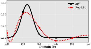
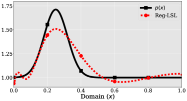
We first apply Reg-LSL to the SISO problem for both the Schrodinger and Helmholtz problems (the Helmholtz equation with positive modeling diffusive electromagnetic problem). We compare the bases after Lanczos orthogonalization to those from the background, the corresponding internal solutions, and the reconstructions of the perturbation. Both problems are discretized on the interval with a background perturbation of for the Schrodinger problem and in the Helmholtz problem. The internal perturbation follows a Gaussian distribution scaled by a constant factor , centered at and with standard deviation . The Dirichlet data is collected at a single point source located at the origin for in the Schrodinger case and in the Helmholtz case. The synthetic data is computed by solving the forward problem using a centered finite difference scheme with step size . The regularization is enforced in both problems by truncating the singular values of the mass matrix for -. For the linear inverse problem in equation (31), we use the Moore-Penrose pseudo inverse with a truncation level of - for both the Schrödinger and Helmholtz problems.
 |
 |
| a) Schrödinger Problem | b) Helmholtz Problem |
Figure 1 illustrates the perturbation and reconstructed solutions for the a) Schrödinger problem and the b) Helmholtz problem. In both problems, we observe excellent reconstructions of the perturbation with few oscillations near the source. The Helmholtz reconstruction is more accurate outside of the support of the perturbation, at which point it begins to deviate due to the difference in conductivity, or equivalently, in the wave speed, affecting the slowness metric.
 |
 |
| a) Schrödinger Problem | b) Helmholtz Problem |
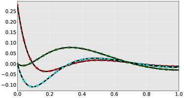
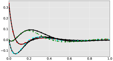
The Lanczos orthogonalized basis functions for the SISO problems are shown in Figure 2. We observe that the basis functions for the perturbed Schrodinger problem are almost exactly the same as those for the background problem; however, the basis functions for the Helmholtz equation deviate from the background basis in the area of the perturbation, again, due to the difference in the travel time metric.
 |
 |
| a) Schrödinger Problem | b) Helmholtz Problem |
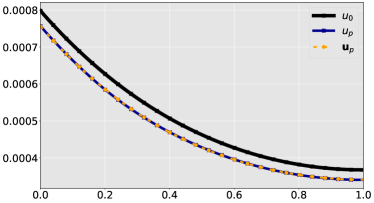
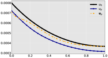
Figure 3 shows the reconstruction of the internal solutions from data using the orthogonalized basis functions. The data generated solution for the Schrödinger problem shown in Figure 3a, is nearly exact. In Figure 3b, the internal solution deviates from the true one at the perturbation. Travel time is not affected in the interval between the source and perturbation, which is why we have an exact reconstruction of the internal solution there. Similarly, a good accuracy of the reconstructions is achieved in the multidimensional setting (see below) with localized conductive perturbations (corresponding to lower wave speed) since they do not affect travel time outside of the perturbation. Low conductivity (high wave-speed) perturbations, however, may work as waveguides, affecting the metrics globally. For this reason, direct LSL would not be applicable for such problems, for which one has to implement iterations [18]
8.2 Reconstructions for the MIMO problem
In this section, we compare reconstructions for the MIMO Schrödinger and Helmholtz problems using Born, LSL, and Reg-LSL. The MIMO problems presented in this work were solved using centered finite difference schemes with symmetrized Laplacian on the domain using a grid step . The Dirichlet data is collected at eight boundary source locations (two at each boundary) at evenly spaced intervals.
8.2.1 Schrödinger Equation
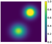
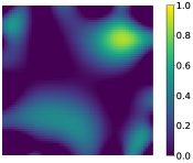
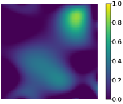
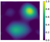
The Schrödinger problem has a background and a perturbation consisting of two Gaussian distributions. The first perturbation is centered at with deviation , and the second is centered at with . For Reg-LSL, the level of regularization is - for the Grammian truncation and - for the LS equation. For Born, the regularization level is -, while the regularization level is - for LSL. The data consists of the frequency set .
 |
 |
 |
 |
| (a) True | (b) Born | (c) LSL | (d) Regularized LSL |
Figure 4 shows the reconstructions of the perturbations using each of the algorithms. We observe that since this is a large number of frequencies for LSL, the standard LSL algorithm has reduced reconstruction quality. Additionally, since this is a moderate contrast problem, the Born reconstruction has significant artifacts. By contrast, Reg-LSL has the lowest level of artifacts and has the highest fidelity to the true perturbation.
8.2.2 Helmholtz problem
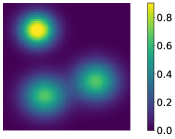
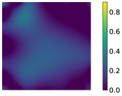
For the quasi-stationary inverse conductivity problem modeled by the Helmholtz equation, we use the background , with a perturbation consisting of three Gaussian distributions. The first distribution is centered at with standard deviation , the second is centered at with standard deviation , and the third is centered at with standard deviation . For Reg-LSL, the Gramian truncation level is -, and the level of regularization for its LS equation is . The regularization levels for inverse Born and standard LSL are - and -, respectively.
 |
 |
 |
 |
| (a) True | (b) Born | (c) LSL | (d) Regularized LSL |
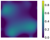
Figure 5 shows the reconstructions of the perturbation in using each of the algorithms. The Born reconstruction has the lowest quality, followed by the standard LSL reconstruction. By contrast, Reg-LSL achieves the best reconstruction of the true perturbation.
8.3 Effects of regularization
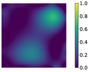
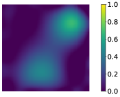
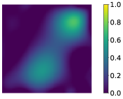
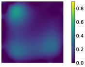
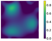
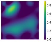
In this section, we analyze the effects of the regularization level on the quality of the reconstructions. Using the same MIMO problem configurations, we consider various thresholds for the regularization of the mass matrix. For both the Schrödinger and Helmholtz problems, we used mass matrix regularization thresholds of -,-,-, and -. For each of these thresholds, the levels of truncation for the linear part of the Schrödinger are -, -, -, - respectively. The levels of truncation for the linear inverse of the Helmholtz problem are -,-,-, and -, respectively.
 |
 |
 |
 |
| (a) - | (b) - | (c) - | (d) - |
Figure 6 compares the increased level of regularization for the Schrödinger problem. We observe that artifacts begin to appear for high and low thresholds. However, the quality is consistent for each of the regularization thresholds.
 |
 |
 |
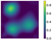 |
| (a) - | (b) - | (c) - | (d) - |
Figure 7 compares the increased level of regularization for the Helmholtz problem. For high regularization thresholds, the resolution is quite low. As the threshold decreases, the accuracy of the reconstruction increases, and the resolution improves.
8.4 Sensitivity Analysis
In this section, we add noise to the data and analyze the sensitivity of the reconstruction to the noise. The perturbation and selection of frequencies are the same as above. The level of truncation for the mass matrix is fixed to - for both Schrödinger and Helmholtz problems. The truncation for the linear inverse problem with and noise was chosen to be -, - and - for the Schrödinger problem and a fixed - for the Helmholtz problem. The noise is sampled from the uniform distribution with a range of and centered at . The percentage of noise is the percent scaling of added to each component of the data.
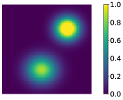 |
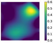 |
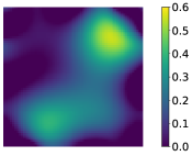 |
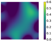 |
| (a) True | (b) 1% Noise | (c) 2% Noise | (d) 5% Noise |
Figure 8 compares the reconstruction of the perturbation as the noise level is increased in the MIMO Schrödinger problem. We observe that as the level of noise increases, there are significant artifacts in the image of the perturbation. However, the Reg-LSL algorithm is able to reconstruct the perturbation well until noise is added.
 |
 |
 |
 |
| (a) True | (b) 1% Noise | (c) 2% Noise | (d) 5% Noise |
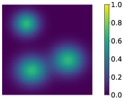
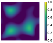
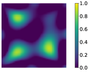
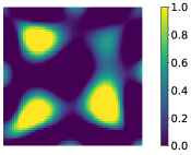
Figure 9 illustrates the reconstructed perturbation using Reg-LSL when noise is added to the data in the MIMO Helmholtz problem.
9 Conclusion
In this work, we introduced a double regularization procedure for the Lippmann-Schwinger-Lanczos method in the frequency domain. This includes a data driven truncation of the mass matrix along with the regularization of the linear integral equation. This allows us to improve reconstructions with larger data sets and handle noisy data. We confirmed this with several numerical experiments.
We also showed here that the Lanczos orthogonalization of the data driven ROM to orthogonalize the frequency domain solutions corresponds precisely to sequential Gram-Schmidt on the corresponding ROM time snapshots. This explains the weak dependence of the orthogonalized snapshots on the medium perturbations for the Schrodinger problem and suggests that the LSL method may work directly for more general formulations. We analyzed several cases of localized conductivity perturbations (corresponding to lower wave speed) in our numerical experiments and showed that while the data-generated internal solutions deviate from the true solutions, the direct reconstructions can still be of high quality.
10 Acknowledgement
The authors gratefully acknowledge support from the Division of Mathematical Sciences at the US National Science Foundation (NSF) through grants DMS-2008441, DMS-2111117, and DMS-2110773, and from the Air Force Office of Scientific Research (AFOSR) through grants FA955020-1-0079 and FA9550-23-1-0220.
References
- [1] H. Ammari, J. Garnier, V. Jugnon, and H. Kang. Direct reconstruction methods in ultrasound imaging of small anomalies. Mathematical Modeling in Biomedical Imaging II: Optical, Ultrasound, and Opto-Acoustic Tomographies, pages 31–55, 2012.
- [2] H. Ammari, S. Moskow, and M. S. Vogelius. Boundary integral formulae for the reconstruction of electric and electromagnetic inhomogeneities of small volume. ESAIM: Control, Optimisation and Calculus of Variations, 9:49–66, 2003.
- [3] A. C. Antoulas. Approximation of large-scale dynamical systems. SIAM, 2005.
- [4] A. C. Antoulas, D. C. Sorensen, and S. Gugercin. A survey of model reduction methods for large-scale systems. Contemporary Mathematics, 280:193–219, 2001.
- [5] Z. Bai. Krylov subspace techniques for reduced-order modeling of large-scale dynamical systems. Applied Numerical Mathematics, 43(1):9 – 44, 2002. 19th Dundee Biennial Conference on Numerical Analysis.
- [6] J. Baker, E. Cherkaev, A. Narayan, and B. Wang. Learning proper orthogonal decomposition of complex dynamics using heavy-ball Neural ODEs. Journal of Scientific Computing, 95(2):54, 2023.
- [7] C. A. Beattie, Z. Drmač, and S. Gugercin. Quadrature-based IRKA for optimal H2 model reduction. IFAC-PapersOnLine, 48(1):5 – 6, 2015. 8th Vienna International Conference on Mathematical Modelling.
- [8] P. Benner, S. Gugercin, and K. Willcox. A survey of projection-based model reduction methods for parametric dynamical systems. SIAM Review, 57(4):483–531, 2015.
- [9] P. Benner, E. Sachs, and S. Volkwein. Model order reduction for PDE constrained optimization. In G. Leugering, editor, Trends in PDE Constrained Optimization, pages 303–326. Springer, 2014.
- [10] H. Bertete-Aguirre, E. Cherkaev, and M. Oristaglio. Non-smooth gravity problem with total variation penalization functional. Geophysical Journal International, 149(2):499–507, 2002.
- [11] G. Beylkin and R. Burridge. Linearized inverse scattering problems in acoustics and elasticity. Wave motion, 12(1):15–52, 1990.
- [12] B. Biondi. 3D seismic imaging. Society of Exploration Geophysicists, 2006.
- [13] N. Bleistein, J. K. Cohen, and J. Stockwell. Mathematics of multidimensional seismic imaging, migration, and inversion, volume 13. Springer, 2001.
- [14] L. Borcea, V. Druskin, and L. Knizhnerman. On the continuum limit of a discrete inverse spectral problem on optimal finite difference grids. Communications on pure and applied mathematics, 58(9):1231–1279, 2005.
- [15] L. Borcea, V. Druskin, A. Mamonov, M. Zaslavsky, and J. Zimmerling. Reduced order model approach to inverse scattering. SIAM Journal on Imaging Sciences, 13(2):685–723, 2020.
- [16] L. Borcea, V. Druskin, A. V. Mamonov, S. Moskow, and M. Zaslavsky. Reduced order models for spectral domain inversion: embedding into the continuous problem and generation of internal data. Inverse Problems, 36(5), 2020.
- [17] L. Borcea, V. Druskin, A. V. Mamonov, and M. Zaslavsky. Robust nonlinear processing of active array data in inverse scattering via truncated reduced order models. Journal of Computational Physics, 381:1–26, 2019.
- [18] L. Borcea, J. Garnier, A. V. Mamonov, and J. Zimmerling. Waveform inversion with a data driven estimate of the internal wave. SIAM Journal on Imaging Sciences, 16(1):280–312, 2023.
- [19] A. Bruckstein, T. Citron, and T. Kailath. Inverse scattering and minimal partial realizations. International Journal of Control, 48(4):1537–1550, 1988.
- [20] F. Cakoni and H. Haddar. Transmission eigenvalues in inverse scattering theory. Inverse Problems and Applications, Inside Out, 2012.
- [21] M. Cheney and B. Borden. Fundamentals of radar imaging, volume 79. SIAM, 2009.
- [22] E. Cherkaev and A. C. Tripp. Inverse conductivity problem for inaccurate measurements. Inverse Problems, 12(6):869, 1996.
- [23] W. C. Chew and Y.-M. Wang. Reconstruction of two-dimensional permittivity distribution using the distorted Born iterative method. IEEE transactions on medical imaging, 9(2):218–225, 1990.
- [24] J. M. Chung, M. E. Kilmer, and D. P. O’Leary. A framework for regularization via operator approximation. SIAM Journal on Scientific Computing, 37(2):B332–B359, 2015.
- [25] D. Colton and R. Kress. Inverse acoustic and electromagnetic scattering theory, volume 93. Springer Science & Business Media, 2013.
- [26] V. Druskin, L. Knizhnerman, and M. Zaslavsky. Solution of large scale evolutionary problems using rational Krylov subspaces with optimized shifts. SIAM Journal on Scientific Computing, 31(5):3760–3780, 2009.
- [27] V. Druskin, A. Mamonov, and M. Zaslavsky. A nonlinear method for imaging with acoustic waves via reduced order model backprojection. SIAM Journal on Imaging Sciences, 11(1):164–196, 2018.
- [28] V. Druskin, A. V. Mamonov, A. E. Thaler, and M. Zaslavsky. Direct, nonlinear inversion algorithm for hyperbolic problems via projection-based model reduction. SIAM Journal on Imaging Sciences, 9(2):684–747, 2016.
- [29] V. Druskin, S. Moskow, and M. Zaslavsky. Lippmann–Schwinger–Lanczos algorithm for inverse scattering problems. Inverse Problems, 37(7):075003, 2021.
- [30] V. Druskin, S. Moskow, and M. Zaslavsky. On extension of the data driven ROM inverse scattering framework to partially nonreciprocal arrays. Inverse Problems, 38(8):084002, 2022.
- [31] V. Druskin, V. Simoncini, and M. Zaslavsky. Solution of the time-domain inverse resistivity problem in the model reduction framework Part i. One-dimensional problem with SISO data. SIAM Journal on Scientific Computing, 35(3):A1621–A1640, 2013.
- [32] P. Feldmann and R. W. Freund. Efficient linear circuit analysis by Padé approximation via the Lanczos process. IEEE Transactions on Computer-Aided Design of Integrated Circuits and Systems, 14(5):639–649, 1995.
- [33] C. Fletcher. Computational Galerkin Methods. Springer, 1984.
- [34] I. V. Gosea, S. Gugercin, and C. Beattie. Data-driven balancing of linear dynamical systems. SIAM Journal on Scientific Computing, 44(1):A554–A582, 2022.
- [35] W. B. Gragg and A. Lindquist. On the partial realization problem. Linear Algebra and its Applications, 50:277–319, 1983.
- [36] E. J. Grimme. Krylov projection methods for model reduction. University of Illinois at Urbana-Champaign, 1997.
- [37] S. Güttel. Rational Krylov approximation of matrix functions: Numerical methods and optimal pole selection. GAMM-Mitteilungen, 36(1):8–31, 2013.
- [38] T. M. Habashy, R. W. Groom, and B. R. Spies. Beyond the Born and Rytov approximations: A nonlinear approach to electromagnetic scattering. Journal of Geophysical Research: Solid Earth, 98(B2):1759–1775, 1993.
- [39] P. C. Hansen. Discrete inverse problems: insight and algorithms. SIAM, 2010.
- [40] K. Kilgore, S. Moskow, and J. C. Schotland. Inverse Born series for diffuse waves. In H. Ammari and H. Kang, editors, Imaging Microstructures: Mathematical and Computational Challenges., Comtemporary Mathematics. American Mathematical Society, 2009.
- [41] M. E. Kilmer, P. C. Hansen, and M. I. Espanol. A projection-based approach to general-form Tikhonov regularization. SIAM Journal on Scientific Computing, 29(1):315–330, 2007.
- [42] M. Kordy, E. Cherkaev, and P. Wannamaker. Adaptive model order reduction for the Jacobian calculation in inverse multi-frequency problem for Maxwell’s equations. Applied Numerical Mathematics, 109:1–18, 2016.
- [43] M. Kordy, E. Cherkaev, and P. Wannamaker. Null space correction and adaptive model order reduction in multi-frequency Maxwell’s problem. Advances in Computational Mathematics, 43:171–193, 2017.
- [44] A. I. Nachman and M. J. Ablowitz. A multidimensional inverse-scattering method. Studies in applied mathematics, 71(3):243–250, 1984.
- [45] B. N. Parlett. Reduction to tridiagonal form and minimal realizations. SIAM Journal on Matrix Analysis and Applications, 13(2):567–593, 1992.
- [46] L. Reichel, F. Sgallari, and Q. Ye. Tikhonov regularization based on generalized Krylov subspace methods. Applied Numerical Mathematics, 62(9):1215–1228, 2012.
- [47] W. W. Symes. Reverse time migration with optimal checkpointing. Geophysics, 72(5):SM213–SM221, 2007.
- [48] C. R. Vogel. Computational methods for inverse problems. SIAM, 2002.
- [49] M. S. Vogelius and D. Volkov. Asymptotic formulas for perturbations in the electromagnetic fields due to the presence of inhomogeneities of small diameter. ESAIM: Mathematical Modelling and Numerical Analysis, 34(4):723–748, 2000.
- [50] K. Willcox and J. Peraire. Balanced model reduction via the proper orthogonal decomposition. AIAA journal, 40(11):2323–2330, 2002.
- [51] J. Zimmerling, V. Druskin, M. Zaslavsky, and R. Remis. Model order reduction of electromagnetic wavefields in open domains. Geophysics, 83(2):1–38, 2017.
- [52] J. Zimmerling, L. Wei, P. Urbach, and R. Remis. A Lanczos model-order reduction technique to efficiently simulate electromagnetic wave propagation in dispersive media. Journal of Computational Physics, 315:348–362, 2016.