Cross Entropy in Deep Learning of Classifiers Is Unnecessary
- ISBE Error is All You Need

Abstract

In deep learning classifiers, the cost function usually takes the form of a combination of SoftMax and CrossEntropy functions. The SoftMax unit transforms the scores predicted by the model network into assessments of the degree (probabilities) of an object’s membership to a given class. On the other hand, CrossEntropy measures the divergence of this prediction from the distribution of target scores. This work introduces the ISBE functionality, justifying the thesis about the redundancy of cross entropy computation in deep learning of classifiers. Not only can we omit the calculation of entropy, but also, during back-propagation, there is no need to direct the error to the normalization unit for its backward transformation. Instead, the error is sent directly to the model’s network. Using examples of perceptron and convolutional networks as classifiers of images from the MNIST collection, it is observed for ISBE that results are not degraded with SoftMax only, but also with other activation functions such as Sigmoid, Tanh, or their hard variants HardSigmoid and HardTanh. Moreover, up to three percent of time is saved within the total time of forward and backward stages. The article is addressed mainly to programmers and students interested in deep model learning. For example, it illustrates in code snippets possible ways to implement ISBE units, but also formally proves that the softmax trick only applies to the class of softmax functions with relocations.

1 Introduction

A deep model is a kind of mental shortcut ([1]), broadly understood as a model created in deep learning of a certain artificial neural network $\mathcal{N}$, designed for a given application. What, then, is an artificial neural network ([2]), its deep learning ([3, 4]), and what applications ([5]) are we interested in?

From a programmer’s perspective, an artificial neural network is a type of data processing algorithm ([6]), in which subsequent steps are carried out by configurable computational units, and the order of processing steps is determined by a directed graph of connections without loops.

At the training stage, each group of input data $X$, i.e., each group of training examples, first undergoes the inference (forward) phase on the current model, i.e., processing through the network $\mathcal{N}$ at its current parameters $W$. As a result, network outputs $Y\leftarrow\mathcal{F}_{\mathcal{N}}(X;W)$ are produced ([7]).

$$\begin{array}[]{l}\displaystyle\overbrace{\xrightarrow{X;\,W}\boxed{\mathcal{F}_{\mathcal{N}}}\xrightarrow{Y\leftarrow\mathcal{F}_{\mathcal{N}}(X;W)}}^{\text{INFERENCE}}\quad\equiv\quad\overbrace{\boxed{\quad\cdots\quad\xrightarrow{X_{u};\,W_{u}}\boxed{\mathcal{F}_{\mathcal{U}}}\xrightarrow{Y_{u}\leftarrow\mathcal{F}_{\mathcal{U}}(X_{u};W_{u})}\quad\cdots\quad}}^{\text{INFERENCE}}\end{array}$$

After the inference phase comes the model update phase, where the current model is modified (improved) according to the selected optimization procedure ([8]). The model update phase begins with calculating the loss (cost) value $Z\leftarrow\mathcal{L}(Y,Y^{\circ})$ defined by the chosen loss function $\mathcal{L}$ as well as the inference outcome $Y$ and the target result $Y^{\circ}$.

$$\begin{array}[]{l}\overbrace{\displaystyle\xrightarrow{X;\,W}\boxed{\mathcal{F}_{\mathcal{N}}}\xrightarrow{Y\leftarrow\mathcal{F}_{\mathcal{N}}(X;W)}}^{\text{INFERENCE}}\quad\cdots\quad\overbrace{\xrightarrow{Y,Y^{\circ}}\boxed{\mathcal{L}}\xrightarrow{Z\leftarrow\mathcal{L}(Y,Y^{\circ})}}^{\text{model update - start}}\end{array}$$

The loss $Z$ depends (indirectly through $Y$) on all parameters $W$, and what conditions the next step of the update phase is the determination of sensitivity $\overline{W}$ of the loss function $\mathcal{L}$ to their changes. The mathematical model of sensitivity is the gradient $\overline{W}\doteq\frac{\partial{\mathcal{L}}}{\partial{W}}$. Knowing this gradient, the optimizer will make the actual modification of $W$ in a direction that also takes into account the values of gradients obtained for previous training batches.

Calculating the gradient with respect to parameters actually assigned to different computational units required the development of an efficient algorithm for its propagation in the opposite direction to inference ([9, 10]).

Just as in the inference phase, each unit $\mathcal{U}$ has its formula $Y_{u}\leftarrow\mathcal{F}_{\mathcal{U}}(X_{u},W_{u})$ for processing data from input $X_{u}$ to output $Y_{u}$ with parameters $W_{u}$, so in the backward gradient propagation phase, it must have a formula $\overline{X}_{u},\overline{W}_{u}\leftarrow\overline{\mathcal{F}}_{\mathcal{U}}(\overline{Y}_{u})$ for transforming the gradients assigned to its outputs $\overline{Y}_{u}$ into gradients assigned to its inputs $\overline{X}_{u}$ and its parameters $\overline{W}_{u}$.

$$\begin{array}[]{c}\overbrace{\xleftarrow{\overline{X};\,\overline{W}\leftarrow\overline{\mathcal{F}}_{\mathcal{N}}(\overline{Y};X,Y,W)}\boxed{\overline{\mathcal{F}}_{\mathcal{N}}}\xleftarrow{\overline{Y}}}^{\text{BACKPROPAGATION}}\quad\cdots\quad\overbrace{\xleftarrow{\overline{Y}\leftarrow\overline{\mathcal{L}}(\overline{Z};Y,Z)}\boxed{\overline{\mathcal{L}}}\xleftarrow{\mathbf{1}=\frac{\partial{Z}}{\partial{Z}}}}^{\text{loss function gradient\,}\frac{\partial{L}}{\partial{Y}}}\\[10.0pt] \overbrace{\boxed{\quad\cdots\quad\xleftarrow{\overline{X}_{u};\,\overline{W}_{u}\leftarrow\overline{\mathcal{F}}_{\mathcal{U}}(\overline{Y}_{u};X_{u},Y_{u},W_{u})}\boxed{\overline{\mathcal{F}}_{\mathcal{U}}}\xleftarrow{\overline{Y}_{u}}\quad\cdots\quad}}^{\text{GRADIENT BACKPROPAGATION}}\end{array}$$

Based on such local rules of gradient backpropagation and the created computation graph, the backpropagation algorithm can determine the gradients of the cost function with respect to each parameter in the network. The computation graph is created during the inference phase and is essentially a stack of links between the arguments and results of calculations performed in successive units ([10, 11]).

Deep learning is precisely a concert of these inference and update phases in the form of gradient propagation, calculated for randomly created groups of training examples. These phases, intertwined, operate on multidimensional deep tensors (arrays) of data, processed with respect to network inputs and on deep tensors of gradient data, processed with respect to losses, determined for the output data of the trained network.

Here, by a deep tensor, we mean a multidimensional data array that has many feature maps, i.e., its size along the feature axis is relatively large, e.g., 500, which means 500 scalar feature maps. We then say that at this point in the network, our data has a deep representation in a 500-dimensional space.

As for the applications we are interested in this work, the answer is those that have at least one requirement for classification ([12]). An example could be crop detection from satellite images ([13]), building segmentation in aerial photos [14], but also text translation ([15]). Classification is also related to voice command recognition ([16]), speaker recognition ([17]), segmentation of the audio track according to speakers ([18]), recognition of speaker emotions with visual support ([19]), but also classification of objects of interest along with their localization in the image ([20]).

It may be risky to say that after 2015, in all the aforementioned deep learning classifiers, the cost function takes the form of a composition of the $SoftMax$ function ([21]) and the $CrossEntropy$ function, i.e., cross-entropy ([22]). The SoftMax unit normalizes the scores predicted by the classifier model for the input object, into softmax scores that sum up to one, which can be treated as an estimation of the conditional probability distribution of classes. Meanwhile, cross-entropy measures the divergence (i.e., divergence) of this estimation from the target probability distribution (class scores). In practice, the target score may be taken from a training set prepared manually by a so-called teacher ([23]) or may be calculated automatically by another model component, e.g., in the knowledge distillation technique ([24]).

For $K$ classes and $n_{b}$ training examples, the $SoftMax$ function is defined for the raw score matrix $X\in\mathbb{R}^{n_{b}\times K}$ as:

$$\left[Y\leftarrow SoftMax(X)\right]\quad\longrightarrow\quad\left[Y_{bi}\leftarrow\frac{e^{X_{bi}}}{\displaystyle\sum_{j\in[K]}e^{X_{bj}}},\,b\in[n_{b}],\,i\in[K]\right]\,,$$

where the notation $[K]$ denotes any $K$-element set of indices - in this case, they are class labels.

The $CrossEntropy$ function on the matrix $Y,Y^{\circ}\in\mathbb{R}^{n_{b}\times K}$ is defined by the formula:

$$\left[Z\leftarrow CrossEntropy(Y,Y^{\circ})\right]\longrightarrow\left[Z_{b}\leftarrow\displaystyle-\sum_{j\in[K]}Y^{\circ}_{bj}\ln Y_{bj},\,b\in[n_{b}],\,z\in\mathbb{R}^{n_{b}}\right]$$

(1) $$\overbrace{\begin{array}[]{l}\overbrace{\xrightarrow{\text{classified object}}\boxed{\mathcal{F}_{\mathcal{N}}}\xrightarrow{\text{raw scores\,}X}}^{\text{SCORES INFERENCE}}\\[5.0pt] \overbrace{\xrightarrow{\text{raw scores\,}X}\boxed{\text{\tt SoftMax}}\xrightarrow{\text{soft scores\,}Y,\,Y^{\circ}}\boxed{\text{\tt CrossEntropy}}\xrightarrow{\text{losses\,}Z}}^{\text{LOSS ESTIMATION\,}\mathcal{L}}\end{array}}^{\text{Classifier loss function: Separated Implementation}}$$

When classifiers began using a separated implementation of the combination of the normalization unit SoftMax and the unit CrossEntropy, it quickly became evident in practice that its implementation had problems with scores close to zero, both in the inference phase and in the backward propagation of its gradient. Only the integration of CrossEntropy with normalization SoftMax eliminated these inconveniences. The integrated approach has the following form:

$$\overbrace{\begin{array}[]{l}\overbrace{\xrightarrow{\text{classified object}}\boxed{\mathcal{F}_{\mathcal{N}}}\xrightarrow{\text{raw scores\,}X}}^{\text{INFERENCE}}\\[7.0pt] \overbrace{\xrightarrow{\text{raw scores\,}X,\text{soft scores\,}Y^{\circ}}\boxed{\text{\tt CrossEntropy\ $\circ$\ SoftMax}}\xrightarrow{\text{losses\,}Z}}^{\text{LOSS ESTIMATION\,}\mathcal{L}}\end{array}}^{\text{Classifier loss function - Integrated Implementation}}$$

The integrated functionality of these two features has the following redundant mathematical notation:

$$\begin{array}[]{l}Z\leftarrow\left[CrossEntropy\,\circ\,SoftMax\right](X,Y^{\circ})\longrightarrow\\[5.0pt] Z_{b}\leftarrow\displaystyle-\sum_{j\in[K]}Y^{\circ}_{bj}\ln\frac{e^{X_{bj}}}{\displaystyle\sum_{i\in[K]}e^{X_{bi}}},\,b\in[n_{b}]\end{array}$$

This redundancy in notation was helpful in deriving the equation for the gradient backpropagation for the integrated loss function $CrossEntropy\,\circ\,SoftMax$ ([25]).

The structure of this paper is as follows:

1. In the second section titled ISBE Functionality, the conditions that a normalization unit must meet for its combination with a cross-entropy unit to have a gradient at the input equal to the difference in soft scores: $\overline{X}=Y-Y^{\circ}$ are analyzed. Then the definition of ISBE functionality is introduced, which in the inference phase (I) normalizes the raw score to a soft score (S), and in the backward propagation phase (B) returns an error (E), equal to the difference in soft scores. It is also justified why in the case of the $SoftMax$ normalization function, the ISBE unit has, from the perspective of the learning process, the functionality of the integrated unit CrossEntropy $\circ$ SoftMax.

2. In the third section, using the example of the problem of recognizing handwritten digits and the standard MNIST(60K) image collection ([26]), numerous experiments show that in addition to the obvious savings in computational resources, in the case of five activations serving as normalization functions, the classifier’s effectiveness is not lower than that of the combination of the normalization unit Softmax and the unit Cross Entropy. This ISBE property was verified for the activation units Softmax, Sigmoid, Hardsigmoid, and Tanh and Hardtanh.

3. The last fourth section contains conclusions.

4. Appendix A, titled Cross-Entropy and Softmax Trick Properties, contains the formulation and proof of the theorem on the properties of the softmax trick.

2 ISBE Functionality

The ISBE functionality is a proposed simplification of the cost function, combining the SoftMax normalization function with the cross-entropy function, hereafter abbreviated as CE_all. Its role is to punish those calculated probability distributions that significantly differ from the distributions of scores proposed by the teacher.

To understand this idea, let’s extend the inference diagram for CE_all with the backward propagation part for the gradient. We consider this diagram in its separated version, omitting earlier descriptions for the diagram (1):

(2) $$\begin{array}[]{l}\overbrace{\xrightarrow{X}\boxed{\text{\tt SoftMax}}\xrightarrow{Y,\,Y^{\circ}}\boxed{\text{\tt CrossEntropy}}\xrightarrow{Z}}^{\text{LOSS INFERENCE\,}\mathcal{L}}\\[10.0pt] \overbrace{\xleftarrow{\overline{X}\xleftarrow{Theorem\,\ref{th:strick}}Y-Y^{\circ}}\boxed{\overline{\text{\tt SoftMax}}}\xleftarrow{\overline{Y};\,Y,\,Y^{\circ}}\boxed{\overline{\text{\tt CrossEntropy}}}\xleftarrow{\overline{Z}=\mathbf{1}}}^{\text{BACKPROPAGATION}}\end{array}$$

The meaning of variables $X,Y,Y^{\circ},Z$ and $\overline{Z},\overline{Y},\overline{X}$ appearing in the above diagram (2):
$\begin{array}[]{ll}X&\text{raw score at the input of the normalization function preceding cross-entropy CE},X\in\mathbb{R}^{K},\\ Y&\text{normalization result, so-called soft score\,,}Y\in(0,1)^{K},\\ Y^{\circ}&\text{target soft score, assigned to the classified example\,,}\\ Z&\text{output of cross-entropy CE\,,}Z\in\mathbb{R},\\ \overline{Z}&\text{formal gradient at the input of the backward propagation algorithm,\,}\overline{Z}=1,\\ \overline{Y}&\text{gradient of cross-entropy CE with respect to Y:\,}\overline{Y}=\frac{\partial{Z}}{\partial{Y}}=-\frac{Y^{\circ}}{Y},\\[3.0pt] \overline{X}&\text{gradient of cross-entropy CE with respect to X:\,}\overline{X}\xleftarrow{Theorem\,\ref{th:strick}}(Y-Y^{\circ})\,.\end{array}$

The key formula here is $\overline{X}\leftarrow(Y-Y^{\circ})$. Its validity comes from the mentioned theorem and the formula (6) associated with the softmax trick property.

The equation (5) on the form of the Jacobian of the normalization unit is both a sufficient and necessary condition for its combination with the cross-entropy unit to ensure the equality (6). Moreover, this condition implies that an activation function with a Jacobian of the softmax type is a SoftMax function with optional relocation.

Theorem 1 leads us to a seemingly pessimistic conclusion: it is not possible to seek further improvements by changing the activation and at the same time expect the softmax trick property to hold. Thus, the question arises: what will happen if, along with changing the activation unit, we change the cross-entropy unit to another, or even omit it entirely?

In the ISBE approach, the aforementioned simplification of the CE_all cost function involves precisely omitting the cross-entropy operation in the inference stage and practically omitting all backward operations for this cost function. So what remains? The answer is also an opportunity to decode the acronym ISBE again:

1. In the inference phase (I), we normalize the raw score $X$ to $Y=SoftMax(X)$, characterized as a soft score (S).

2. In the backward propagation phase (B), we return an error (E) equal to the difference between the calculated soft score and the target score, i.e., $\overline{X}\doteq Y-Y^{\circ}$.

Why can we do this and still consider that in the case of the SoftMax activation function, the value of the gradient transmitted to the network is identical: $\overline{X}_{CE_{all}}=\overline{X}_{ISBE}\doteq Y-Y^{\circ}$?

The answer comes directly from the property $\overline{X}_{CE_{all}}=Y-Y^{\circ}$, formulated in equation (6), which was defined in the theorem 1 as the softmax trick property.

We thus have on the left the following diagram of data and gradient backpropagation through such a unit. On the right we have its generalization to a ScoreNormalization unit instead of SoftMax unit.

$$\left.\begin{array}[]{l}\overbrace{\xrightarrow{X}\boxed{\text{\tt SoftMax}}\xrightarrow{Y,\,Y^{\circ}}}^{\text{ISBE INFERENCE}}\\[7.0pt] \overbrace{\xleftarrow{\overline{X}\leftarrow Y-Y^{\circ}}\boxed{{\text{\tt Subtract}}}\xleftarrow{Y,\,Y^{\circ}}}^{\text{$\overline{ISBE}$\, BACKPROPAGATION}}\end{array}\right\}\xrightarrow{\text{generalize}}\left\{\begin{array}[]{l}\overbrace{\xrightarrow{X}\boxed{\text{\tt Score\,Normalization}}\xrightarrow{Y,\,Y^{\circ}}}^{\text{ISBE INFERENCE}}\\[7.0pt] \overbrace{\xleftarrow{\overline{X}\leftarrow Y-Y^{\circ}}\boxed{{\text{\tt Subtract}}}\xleftarrow{Y,\,Y^{\circ}}}^{\text{$\overline{ISBE}$\, BACKPROPAGATION}}\end{array}\right.$$

Which activation functions should we reach for in order to test them in the ISBE technique?

1. The SoftMax activation function should be the first candidate for comparison, as it theoretically guarantees behavior comparable to the system containing cross-entropy.

2. Activations should be monotonic, so that the largest value of the raw score remains the largest score in the soft score sequence.

3. Soft scores should be within a limited range, e.g., $[0,1]$ as in the case of SoftMax and Sigmoid, or $[-1,+1]$ as for Tanh.

4. The activation function should not map two close scores to distant scores. For example, normalizing a vector of scores by projecting onto a unit sphere in the $p$-th Minkowski norm meets all above conditions, however, it is not stable around zero. Normalization $\frac{x}{\|x\|_{p}}$ maps, for example, two points $\epsilon,-\epsilon$ distant by $2\cdot\|\epsilon\|_{p}$ to points distant exactly by $2$, thus changing their distance $\frac{1}{\|\epsilon\|_{p}}$ times, e.g., a million times, when $\|\epsilon\|_{p}=10^{-6}$. This operation is known in Pytorch library as normalize function.

The experiments conducted confirm the validity of the above recommendations. The Pytorch library functions softmax, sigmoid, tanh, hardsigmoid, hardtanh meet the above three conditions and provide effective classification at a level of effectiveness higher than $99.5\%$, comparable to CrossEntropy $\circ$ SoftMax. In contrast, the function normalize gave results over $10\%$ worse - on the same MNIST(60K) collection and with the same architectures.

What connects these good normalization functions $F:\mathbb{R}^{K}\rightarrow\mathbb{R}^{K}$, of which two are not even fully differentiable? Certainly, it is the Lipschitz condition occurring in a certain neighborhood of zero ([27]):

$$x\in\mathbb{R}^{K},\ \|x\|_{p}\leq\epsilon\longrightarrow\|F(x)\|_{p}\leq c\|x\|_{p}\,,\quad\text{where $c$ is a certain constant\,.}$$

Note that the Lipschitz condition meets the expectations of the fourth requirement on the above list of recommendations for ISBE. Moreover, we do not expect here that the constant $c$ be less than one, i.e., that the function $F$ has a narrowing character.

We need also a recommendation for teachers preparing class labels, which we represent as vectors blurred around the base vectors of axes $I_{K}=[e_{1},\dots,e_{K}],\ e_{i}[j]\doteq\delta_{ij}$:

1. example blurring value $\mu$, e.g., $\mu=10^{-6}$:

   $$\tilde{e}_{i}[j]\leftarrow(1-\mu)\delta_{ij}+\frac{\mu}{K-1}(1-\delta_{ij})$$

2. when the range of activation values is other than the interval $[0,1]$, we adjust the vector $\tilde{e}_{i}$ to the new range, e.g., for tanh the range is the interval $(-1,+1)$ and then the adjustment has the form:

   $$\tilde{e}_{i}\leftarrow 2\cdot\tilde{e}_{i}-1,\ i=1,\dots,K$$

Finally, let’s take a look at the code for the main loop of the program implemented on the Pytorch platform.

1. This is what the code looks like when loss_function is chosen as nn.CrossEntropyLoss:

   for (labels,images) in tgen:
       outputs = net(images)
       loss = loss_function(outputs, labels)
       optimizer.zero_grad()
       loss.backward()
       optimizer.step()
   

2. Now we introduce the ISBE option for SoftMax activation:

   for (labels,images) in tgen:
       outputs = net(images)
       if no_cross_entropy:
           soft_error = softmax(outputs) - labels
           optimizer.zero_grad()
           outputs.backward(soft_error)
       else:
           loss = loss_function(outputs, labels)
           optimizer.zero_grad()
           loss.backward()
       optimizer.step()
   

3. If we want to test more options, the loop code will extend a bit:

   for (labels,images) in tgen:
       outputs = net(images)
       if no_cross_entropy:
           if soft_option=="softmax":
               soft_error = softmax(outputs) - labels
           if soft_option=="tanh":
               soft_error = tanh(outputs) - (2.*labels-1.)
           elif soft_option=="hardtanh":
               soft_error = hardtanh(outputs) - (2.*labels-1.)
           elif # ...
                # next options
           optimizer.zero_grad()
           outputs.backward(soft_error)
       else:
           loss = loss_function(outputs, labels)
           optimizer.zero_grad()
           loss.backward()
       optimizer.step()
   

4. If we prefer to have a visually shorter loop, then by introducing the variable soft_function and extending the class DataProvider with matching target labels for a given soft option, we finally get a compact form:

   for (labels,images) in tgen:
       outputs = net(images)
       if no_cross_entropy:
           soft_error = soft_function(outputs) - labels
           optimizer.zero_grad()
           outputs.backward(soft_error)
       else:
           loss = loss_function(outputs, labels)
           optimizer.zero_grad()
           loss.backward()
       optimizer.step()
   

Of course, the above code snippets are only intended to illustrate how easy it is to add the functionality of ISBE to an existing application.

3 Experiments

What do we want to learn from the planned experiments? We already know from theory that in the case of the SoftMax activation, we cannot worsen the parameters of the classifier using cross-entropy, both in terms of success rate and learning time.

Therefore, we first want to verify whether theory aligns with practice, but also to check for which normalization functions the ISBE unit does not degrade the model’s effectiveness compared to CE_all.

The learning time $t_{ISBE}$ should be shorter than $t_{CE}$, but to be independent of the specific implementation, we will compare the percentage of the backpropagation time in the total time of inference and backpropagation:

(3) $$\tau\doteq\frac{\text{backpropagation time}}{\text{inference time}+\text{backpropagation time}}\cdot 100\%$$

We evaluate the efficiency of the ISBE idea on the standard MNIST(60K) image collection and the problem of their classification.

From many quality metrics, we choose the success rate (also called accuracy), defined as the percentage of correctly classified elements from the test collection MNIST(10K)

(4) $$\alpha=\frac{\text{number of correct classifications}}{\text{size of the test collection}}\cdot 100\%$$

We want to know how this value changes when we choose different architectures, different activations in the ISBE technique, but also different options for aggregating cross-entropy over the elements of the training batch. Thus, we have the following degrees of freedom in our experiments:

1. Two architecture options

   • Architecture $\mathcal{N}_{0}$ consists of two convolutions $\kern-4.0pt\begin{array}[]{r}\kern 0.0pt\raisebox{0.0pt}{$\mbox{\tiny$$}$}\\ \kern 0.0pt\raisebox{0.0pt}{$\mbox{\tiny$$}$}\end{array}\kern-12.0pt\begin{array}[]{c}\mbox{\huge$\mathbb{C}$}\\[-18.0pt] \kern 8.0pt\raisebox{0.0pt}{$\mbox{\tiny$$}$}\end{array}\kern-8.0pt\begin{array}[]{l}\kern-2.5pt\raisebox{0.0pt}{$\mbox{\tiny$$}$}\\ \kern-2.5pt\raisebox{0.0pt}{$\mbox{\tiny$$}$}\end{array}$ and two linear units $\kern-6.0pt\begin{array}[]{r}\kern 0.0pt\raisebox{0.0pt}{$\mbox{\tiny$$}$}\\ \kern 0.0pt\raisebox{0.0pt}{$\mbox{\tiny$$}$}\end{array}\kern-14.0pt\begin{array}[]{c}\mbox{\huge$\mathbb{F}$}\\[-17.0pt] \kern 16.0pt\raisebox{0.0pt}{$\mbox{\tiny$$}$}\end{array}\kern-17.0pt\begin{array}[]{l}\kern 5.0pt\raisebox{1.0pt}{$\mbox{\tiny$$}$}\\ \kern 2.0pt\raisebox{-1.0pt}{$\mbox{\tiny$$}$}\end{array}$, of which the last one is a projection from the space of deep feature vectors of dimension $512$ to the space of raw scores for each of the $K=10$ classes:

     $$\xrightarrow{\text{\small image}}\kern-4.0pt\begin{array}[]{r}\kern 0.0pt\raisebox{0.0pt}{$\mbox{\tiny$$}$}\\ \kern 0.0pt\raisebox{0.0pt}{$\mbox{\tiny$$}$}\end{array}\kern-15.0pt\begin{array}[]{c}\mbox{\huge$\mathcal{I}$}\\[-17.0pt] \kern 12.0pt\raisebox{0.0pt}{$\mbox{\tiny$$}$}\end{array}\kern-14.0pt\begin{array}[]{l}\kern 5.0pt\raisebox{1.0pt}{$\mbox{\tiny$1$}$}\\ \kern 2.0pt\raisebox{-1.0pt}{$\mbox{\tiny$\kern-2.0pt28_{yx}$}$}\end{array}\kern-4.0pt\begin{array}[]{r}\kern 0.0pt\raisebox{0.0pt}{$\mbox{\tiny$$}$}\\ \kern 0.0pt\raisebox{0.0pt}{$\mbox{\tiny$$}$}\end{array}\kern-12.0pt\begin{array}[]{c}\mbox{\huge$\mathbb{C}$}\\[-18.0pt] \kern 8.0pt\raisebox{0.0pt}{$\mbox{\tiny$$}$}\end{array}\kern-8.0pt\begin{array}[]{l}\kern-2.5pt\raisebox{0.0pt}{$\mbox{\tiny$32$}$}\\ \kern-2.5pt\raisebox{0.0pt}{$\mbox{\tiny$3^{k}2^{s}$}$}\end{array}\kern-4.0pt\begin{array}[]{r}\kern 0.0pt\raisebox{0.0pt}{$\mbox{\tiny$$}$}\\ \kern 0.0pt\raisebox{0.0pt}{$\mbox{\tiny$$}$}\end{array}\kern-12.0pt\begin{array}[]{c}\mbox{\huge$\mathbb{C}$}\\[-18.0pt] \kern 8.0pt\raisebox{0.0pt}{$\mbox{\tiny$$}$}\end{array}\kern-8.0pt\begin{array}[]{l}\kern-2.5pt\raisebox{0.0pt}{$\mbox{\tiny$64$}$}\\ \kern-2.5pt\raisebox{0.0pt}{$\mbox{\tiny$3^{k}2^{s}$}$}\end{array}\kern-2.0pt\begin{array}[]{r}\kern 0.0pt\raisebox{0.0pt}{$\mbox{\tiny$$}$}\\ \kern 0.0pt\raisebox{0.0pt}{$\mbox{\tiny$$}$}\end{array}\kern-15.0pt\begin{array}[]{c}\mbox{\huge$\mathbb{D}$}\\[-17.0pt] \kern 2.0pt\raisebox{0.0pt}{$\mbox{\tiny$$}$}\end{array}\kern-18.0pt\begin{array}[]{l}\kern 0.0pt\raisebox{0.0pt}{$\mbox{\tiny$$}$}\\ \kern 5.0pt\raisebox{-1.0pt}{$\mbox{\tiny$20$}$}\end{array}\kern-6.0pt\begin{array}[]{r}\kern 0.0pt\raisebox{0.0pt}{$\mbox{\tiny$$}$}\\ \kern 0.0pt\raisebox{0.0pt}{$\mbox{\tiny$$}$}\end{array}\kern-14.0pt\begin{array}[]{c}\mbox{\huge$\mathbb{F}$}\\[-17.0pt] \kern 16.0pt\raisebox{0.0pt}{$\mbox{\tiny$$}$}\end{array}\kern-17.0pt\begin{array}[]{l}\kern 5.0pt\raisebox{1.0pt}{$\mbox{\tiny$512$}$}\\ \kern 2.0pt\raisebox{-1.0pt}{$\mbox{\tiny$$}$}\end{array}\kern-6.0pt\begin{array}[]{r}\kern 0.0pt\raisebox{0.0pt}{$\mbox{\tiny$$}$}\\ \kern 0.0pt\raisebox{0.0pt}{$\mbox{\tiny$$}$}\end{array}\kern-14.0pt\begin{array}[]{c}\mbox{\huge$\mathbb{F}$}\\[-17.0pt] \kern 16.0pt\raisebox{0.0pt}{$\mbox{\tiny$$}$}\end{array}\kern-17.0pt\begin{array}[]{l}\kern 5.0pt\raisebox{1.0pt}{$\mbox{\tiny$10$}$}\\ \kern 2.0pt\raisebox{-1.0pt}{$\mbox{\tiny$$}$}\end{array}\xrightarrow{\text{\small class\ scores}}$$

     as by STNN notation ([28]), for instance
     $\left\{\begin{array}[]{cl}\kern-4.0pt\begin{array}[]{r}\kern 0.0pt\raisebox{0.0pt}{$\mbox{\tiny$$}$}\\ \kern 0.0pt\raisebox{0.0pt}{$\mbox{\tiny$$}$}\end{array}\kern-12.0pt\begin{array}[]{c}\mbox{\huge$\mathbb{C}$}\\[-18.0pt] \kern 8.0pt\raisebox{0.0pt}{$\mbox{\tiny$$}$}\end{array}\kern-8.0pt\begin{array}[]{l}\kern-2.5pt\raisebox{0.0pt}{$\mbox{\tiny$32$}$}\\ \kern-2.5pt\raisebox{0.0pt}{$\mbox{\tiny$3^{k}2^{s}$}$}\end{array}&\text{means 32 convolutions with 3x3 masks, sampled with a stride of 2},\\ \kern-2.0pt\begin{array}[]{r}\kern 0.0pt\raisebox{0.0pt}{$\mbox{\tiny$$}$}\\ \kern 0.0pt\raisebox{0.0pt}{$\mbox{\tiny$$}$}\end{array}\kern-15.0pt\begin{array}[]{c}\mbox{\huge$\mathbb{D}$}\\[-17.0pt] \kern 2.0pt\raisebox{0.0pt}{$\mbox{\tiny$$}$}\end{array}\kern-18.0pt\begin{array}[]{l}\kern 0.0pt\raisebox{0.0pt}{$\mbox{\tiny$$}$}\\ \kern 5.0pt\raisebox{-1.0pt}{$\mbox{\tiny$20$}$}\end{array}&\text{DropOut - a unit zeroing 20\% of tensor elements},\\ \kern-6.0pt\begin{array}[]{r}\kern 0.0pt\raisebox{0.0pt}{$\mbox{\tiny$$}$}\\ \kern 0.0pt\raisebox{0.0pt}{$\mbox{\tiny$$}$}\end{array}\kern-14.0pt\begin{array}[]{c}\mbox{\huge$\mathbb{F}$}\\[-17.0pt] \kern 16.0pt\raisebox{0.0pt}{$\mbox{\tiny$$}$}\end{array}\kern-17.0pt\begin{array}[]{l}\kern 5.0pt\raisebox{1.0pt}{$\mbox{\tiny$512$}$}\\ \kern 2.0pt\raisebox{-1.0pt}{$\mbox{\tiny$$}$}\end{array}&\text{a linear unit with a matrix $A\in\mathbb{R}^{?\times 512}$},\\ &\text{here $?=64$ - it is derived from the shape of}\\ &\text{the tensor produced by the previous unit\,.}\end{array}\right.$

   • Architecture $\mathcal{N}_{1}$ consists of two blocks, each with 3 convolutions - it is a purely convolutional network, except for the final projection:

     $$\begin{array}[]{l}\xrightarrow{\text{\small image}}\kern-4.0pt\begin{array}[]{r}\kern 0.0pt\raisebox{0.0pt}{$\mbox{\tiny$$}$}\\ \kern 0.0pt\raisebox{0.0pt}{$\mbox{\tiny$$}$}\end{array}\kern-15.0pt\begin{array}[]{c}\mbox{\huge$\mathcal{I}$}\\[-17.0pt] \kern 12.0pt\raisebox{0.0pt}{$\mbox{\tiny$$}$}\end{array}\kern-14.0pt\begin{array}[]{l}\kern 5.0pt\raisebox{1.0pt}{$\mbox{\tiny$1$}$}\\ \kern 2.0pt\raisebox{-1.0pt}{$\mbox{\tiny$\kern-2.0pt28_{yx}$}$}\end{array}\ \kern-4.0pt\begin{array}[]{r}\kern 0.0pt\raisebox{0.0pt}{$\mbox{\tiny$$}$}\\ \kern 0.0pt\raisebox{0.0pt}{$\mbox{\tiny$$}$}\end{array}\kern-12.0pt\begin{array}[]{c}\mbox{\huge$\mathbb{C}$}\\[-18.0pt] \kern 8.0pt\raisebox{0.0pt}{$\mbox{\tiny$$}$}\end{array}\kern-8.0pt\begin{array}[]{l}\kern-2.5pt\raisebox{0.0pt}{$\mbox{\tiny$32$}$}\\ \kern-2.5pt\raisebox{0.0pt}{$\mbox{\tiny$3^{k}$}$}\end{array}\kern-4.0pt\begin{array}[]{r}\kern 0.0pt\raisebox{0.0pt}{$\mbox{\tiny$$}$}\\ \kern 0.0pt\raisebox{0.0pt}{$\mbox{\tiny$$}$}\end{array}\kern-12.0pt\begin{array}[]{c}\mbox{\huge$\mathbb{C}$}\\[-18.0pt] \kern 8.0pt\raisebox{0.0pt}{$\mbox{\tiny$$}$}\end{array}\kern-8.0pt\begin{array}[]{l}\kern-2.5pt\raisebox{0.0pt}{$\mbox{\tiny$32$}$}\\ \kern-2.5pt\raisebox{0.0pt}{$\mbox{\tiny$3^{k}$}$}\end{array}\kern-4.0pt\begin{array}[]{r}\kern 0.0pt\raisebox{0.0pt}{$\mbox{\tiny$$}$}\\ \kern 0.0pt\raisebox{0.0pt}{$\mbox{\tiny$p$}$}\end{array}\kern-12.0pt\begin{array}[]{c}\mbox{\huge$\mathbb{C}$}\\[-18.0pt] \kern 8.0pt\raisebox{0.0pt}{$\mbox{\tiny$$}$}\end{array}\kern-8.0pt\begin{array}[]{l}\kern-2.5pt\raisebox{0.0pt}{$\mbox{\tiny$32$}$}\\ \kern-2.5pt\raisebox{0.0pt}{$\mbox{\tiny$5^{k}2^{s}$}$}\end{array}\ \kern-2.0pt\begin{array}[]{r}\kern 0.0pt\raisebox{0.0pt}{$\mbox{\tiny$$}$}\\ \kern 0.0pt\raisebox{0.0pt}{$\mbox{\tiny$$}$}\end{array}\kern-15.0pt\begin{array}[]{c}\mbox{\huge$\mathbb{D}$}\\[-17.0pt] \kern 2.0pt\raisebox{0.0pt}{$\mbox{\tiny$$}$}\end{array}\kern-18.0pt\begin{array}[]{l}\kern 0.0pt\raisebox{0.0pt}{$\mbox{\tiny$$}$}\\ \kern 5.0pt\raisebox{-1.0pt}{$\mbox{\tiny$40$}$}\end{array}\kern-4.0pt\begin{array}[]{r}\kern 0.0pt\raisebox{0.0pt}{$\mbox{\tiny$$}$}\\ \kern 0.0pt\raisebox{0.0pt}{$\mbox{\tiny$$}$}\end{array}\kern-12.0pt\begin{array}[]{c}\mbox{\huge$\mathbb{C}$}\\[-18.0pt] \kern 8.0pt\raisebox{0.0pt}{$\mbox{\tiny$$}$}\end{array}\kern-8.0pt\begin{array}[]{l}\kern-2.5pt\raisebox{0.0pt}{$\mbox{\tiny$64$}$}\\ \kern-2.5pt\raisebox{0.0pt}{$\mbox{\tiny$3^{k}$}$}\end{array}\kern-4.0pt\begin{array}[]{r}\kern 0.0pt\raisebox{0.0pt}{$\mbox{\tiny$$}$}\\ \kern 0.0pt\raisebox{0.0pt}{$\mbox{\tiny$$}$}\end{array}\kern-12.0pt\begin{array}[]{c}\mbox{\huge$\mathbb{C}$}\\[-18.0pt] \kern 8.0pt\raisebox{0.0pt}{$\mbox{\tiny$$}$}\end{array}\kern-8.0pt\begin{array}[]{l}\kern-2.5pt\raisebox{0.0pt}{$\mbox{\tiny$64$}$}\\ \kern-2.5pt\raisebox{0.0pt}{$\mbox{\tiny$3^{k}$}$}\end{array}\kern-4.0pt\begin{array}[]{r}\kern 0.0pt\raisebox{0.0pt}{$\mbox{\tiny$$}$}\\ \kern 0.0pt\raisebox{0.0pt}{$\mbox{\tiny$p$}$}\end{array}\kern-12.0pt\begin{array}[]{c}\mbox{\huge$\mathbb{C}$}\\[-18.0pt] \kern 8.0pt\raisebox{0.0pt}{$\mbox{\tiny$$}$}\end{array}\kern-8.0pt\begin{array}[]{l}\kern-2.5pt\raisebox{0.0pt}{$\mbox{\tiny$64$}$}\\ \kern-2.5pt\raisebox{0.0pt}{$\mbox{\tiny$5^{k}2^{s}$}$}\end{array}\ \kern-2.0pt\begin{array}[]{r}\kern 0.0pt\raisebox{0.0pt}{$\mbox{\tiny$$}$}\\ \kern 0.0pt\raisebox{0.0pt}{$\mbox{\tiny$$}$}\end{array}\kern-15.0pt\begin{array}[]{c}\mbox{\huge$\mathbb{D}$}\\[-17.0pt] \kern 2.0pt\raisebox{0.0pt}{$\mbox{\tiny$$}$}\end{array}\kern-18.0pt\begin{array}[]{l}\kern 0.0pt\raisebox{0.0pt}{$\mbox{\tiny$$}$}\\ \kern 5.0pt\raisebox{-1.0pt}{$\mbox{\tiny$40$}$}\end{array}\kern-4.0pt\begin{array}[]{r}\kern 0.0pt\raisebox{0.0pt}{$\mbox{\tiny$$}$}\\ \kern 0.0pt\raisebox{0.0pt}{$\mbox{\tiny$$}$}\end{array}\kern-12.0pt\begin{array}[]{c}\mbox{\huge$\mathbb{C}$}\\[-18.0pt] \kern 8.0pt\raisebox{0.0pt}{$\mbox{\tiny$$}$}\end{array}\kern-8.0pt\begin{array}[]{l}\kern-2.5pt\raisebox{0.0pt}{$\mbox{\tiny$128$}$}\\ \kern-2.5pt\raisebox{0.0pt}{$\mbox{\tiny$4^{k}$}$}\end{array}\kern-6.0pt\begin{array}[]{r}\kern 0.0pt\raisebox{0.0pt}{$\mbox{\tiny$$}$}\\ \kern 0.0pt\raisebox{0.0pt}{$\mbox{\tiny$$}$}\end{array}\kern-14.0pt\begin{array}[]{c}\mbox{\huge$\mathbb{F}$}\\[-17.0pt] \kern 16.0pt\raisebox{0.0pt}{$\mbox{\tiny$$}$}\end{array}\kern-17.0pt\begin{array}[]{l}\kern 5.0pt\raisebox{1.0pt}{$\mbox{\tiny$10$}$}\\ \kern 2.0pt\raisebox{-1.0pt}{$\mbox{\tiny$$}$}\end{array}\xrightarrow{\text{\small class\ scores}}\\ \end{array}$$

     Note that the last convolution in each block has a p requirement for padding, i.e., filling the domain of the image with additional lines and rows so that the image resolution does not change.

2. Three options for reducing the vector of losses in the CrossEntropyLoss unit: none, mean, sum.

3. Five options for activation functions used in the ISBE technique:

   • SoftMax: $\displaystyle y_{i}\leftarrow\frac{e^{x_{i}}}{\displaystyle\sum_{j\in[K]}e^{x_{j}}},\quad i\in[K],$

   • Tanh: $\displaystyle y_{i}\leftarrow\frac{e^{x_{i}}-e^{-x_{i}}}{e^{x_{i}}+e^{-x_{i}}},\quad i\in[K],$

   • HardTanh: $\displaystyle y_{i}\leftarrow\left\{\begin{array}[]{cl}-1&\text{if }x_{i}\leq-1\\ x_{i}&\text{if }-1<x_{i}<+1\\ +1&\text{if }+1\leq x_{i}\end{array}\right\},\quad i\in[K],$

   • Sigmoid: $\displaystyle y_{i}\leftarrow\frac{1}{1+e^{-x_{i}}},\ i\in[K],$

   • HardSigmoid: $\displaystyle y_{i}\leftarrow\left\{\begin{array}[]{cl}0&\text{gdy }x_{i}\leq-2\\ \frac{x_{i}+2}{4}&\text{gdy }-2<x_{i}<+2\\ +1&\text{gdy }+2\leq x_{i}\end{array}\right\}=\frac{HardTanh(x_{i}/2)+1}{2},\quad i\in[K].$

The results of the experiments, on the one hand, confirm our assumption that the conceptual Occam’s razor, i.e., the omission of the cross-entropy unit, results in time savings $\tau$, and on the other hand, the results are surprisingly positive with an improvement in the metric of success rate $\alpha$ in the case of hard activation functions $HardTanh$ and $HardSigmoid$. It was observed that only the option of reduction by none behaves exactly according to theory, i.e., the success rate is identical to the model using $SoftMax$ normalization. Options mean and sum for the model with entropy are slightly better than the model with softmax.

The consistency of models in this case means that the number of images incorrectly classified out of 10 thousand is the same. In the experiments, it was not checked whether it concerns the same images. A slight improvement, in this case, meant that there were less than a few or a dozen errors, and the efficiency of the model above $99.6\%$ meant at most $40$ errors per $10$ thousand of test images.

3.1 Comparison of time complexity

We compare time complexity according to the metric given by the formula (3).

Table 1: Comparison of the metric $\tau$, i.e., the percentage share of backpropagation time in the total time with inference. The share $\tau_{CE}$ of cross-entropy with three types of reduction is compared with five functions of soft normalization. The analysis was performed for architectures $\mathcal{N}_{0}$ and $\mathcal{N}_{1}$.

net mean none sum hsigmoid htanh sigmoid softmax tanh $\mathcal{N}_{0}$ 60.61% 59.56% 59.98% 58.31% 58.21% 57.38% 57.45% 59.07% $\mathcal{N}_{1}$ 54.89% 53.92% 53.98% 52.68% 52.33% 51.75% 51.95% 52.11% $\mathcal{N}_{1}^{r}$ 54.45% 53.92% 54.00% 52.78% 52.30% 51.67% 51.73% 52.11%

Table 2: Metric $\Delta\tau\doteq\tau_{ISBE}-\tau_{CE}$, i.e., the decrease in the percentage share of backpropagation time in the total time with inference. The analysis was performed for architectures $\mathcal{N}_{0}$ and $\mathcal{N}_{1}$.

net CE loss hsigmoid htanh sigmoid softmax tanh $\mathcal{N}_{0}$ mean -2.30% -2.40% -3.23% -3.16% -1.54% $\mathcal{N}_{0}$ none -1.25% -1.35% -2.18% -2.11% -0.50% $\mathcal{N}_{0}$ sum -1.67% -1.77% -2.60% -2.53% -0.92% $\mathcal{N}_{1}$ mean -2.21% -2.56% -3.14% -2.94% -2.79% $\mathcal{N}_{1}$ none -1.24% -1.59% -2.17% -1.97% -1.82% $\mathcal{N}_{1}$ sum -1.30% -1.65% -2.23% -2.03% -1.87%

In the context of time, the table 1 clearly shows that the total time share of backpropagation, obviously depending on the complexity of the architecture, affects the time savings of the ISBE technique compared to CrossEntropyLoss - table 2. The absence of pluses in this table, i.e., the fact that all solutions based on ISBE are relatively faster in the learning phase, is an undeniable fact.

The greatest decrease in the share of backpropagation, over $3\%$, occurs for the $Sigmoid$ and $SoftMax$ activations. The smallest decrease in architecture $\mathcal{N}_{0}$ is noted for the soft (soft) normalization function $Tanh$ and its hard version $HardTanh$. This decrease refers to cross-entropy without reduction, which is an aggregation of losses calculated for all training examples in a given group, into one numerical value.

Inspired by the theorem 1 , which states that the relocation of the $SoftMax$ function preserves the softmax trick property, we also add data to the table 1 for the network $\mathcal{N}_{1}^{r}$. This network differs from the $\mathcal{N}_{1}$ network only in that the normalization unit has a trained relocation parameter. In practice, we accomplish training with relocation for normalization by training with the relocation of the linear unit immediately preceding it. This is done by setting its parameter: bias=True.

As we can see, the general conclusion about the advantage of the ISBE technique in terms of time reducing for the model with the relocation of the normalization function, is the same.

3.2 Comparison of classifier accuracy

Comparison of classifier accuracy and differences in this metric are contained in tables 3 and 4. The accuracy is computed according the formula (4).

The number of pluses on the side of ISBE clearly exceeds the number of minuses. The justification for this phenomenon requires separate research. Some light will be shed on this aspect by the analysis of learning curves - the variance in the final phase of learning is clearly lower. The learning process is more stable.

Table 3: In the table, the success rate of three classifiers based on cross-entropy with different aggregation options is compared with the success rate determined for five options of soft score normalization functions. The analysis was performed for architectures $\mathcal{N}_{0}$ and $\mathcal{N}_{1}$.

net mean none sum hsigmoid htanh sigmoid softmax tanh $\mathcal{N}_{0}$ 99.45% 99.41% 99.47% 99.50% 99.50% 99.56% 99.41% 99.45% $\mathcal{N}_{1}$ 99.61% 99.58% 99.59% 99.64% 99.66% 99.64% 99.62% 99.63% $\mathcal{N}_{1}^{r}$ 99.55% 99.64% 99.64% 99.61% 99.66% 99.69% 99.63% 99.57%

Table 4: Change in success rate between models with cross-entropy and models with soft score normalization function. The analysis was performed for architectures $\mathcal{N}_{0}$ and $\mathcal{N}_{1}$.

net CE loss hsigmoid htanh sigmoid softmax tanh $\mathcal{N}_{0}$ mean 0.05% 0.05% 0.11% -0.04% 0.00% $\mathcal{N}_{0}$ none 0.09% 0.09% 0.15% 0.00% 0.00% $\mathcal{N}_{0}$ sum 0.13% 0.03% 0.09% -0.06% -0.02% $\mathcal{N}_{1}$ mean 0.03% 0.05% 0.03% 0.01% 0.02% $\mathcal{N}_{1}$ none 0.06% 0.08% 0.06% 0.04% 0.05% $\mathcal{N}_{1}$ sum 0.05% 0.07% 0.05% 0.03% 0.04%

In the table 4, we observe that, with the exception of the function $SoftMax$, which on several images of digits performed worse than the model with cross-entropy, the soft activations have an efficiency slightly or significantly better. However, we are talking about levels of tenths or hundredths of a percent here. The largest difference noted for the option softmax was $15$ hundredths of a percent, meaning $15$ more images correctly classified. Such differences are within the margin of statistical error.

The use of relocation for the normalization functionof does not provide a clear conclusion - for some models there is a slight improvement, for others a slight deterioration. It is true that the ISBE unit with sigmoid activation achieved the best efficiency of $99.69\%$, but this is only a matter of a few images.

Within the limits of statistical error, we can say that the ISBE technique gives the same results in recognizing MNIST classes. Its advantages are:

• of decrease time in the total time,

• simplification of architecture, and therefore plaing the philosophical role of Occam’s razor.

3.3 Visual analysis

Further analysis of the results will be based on the visual comparison of learning curves.

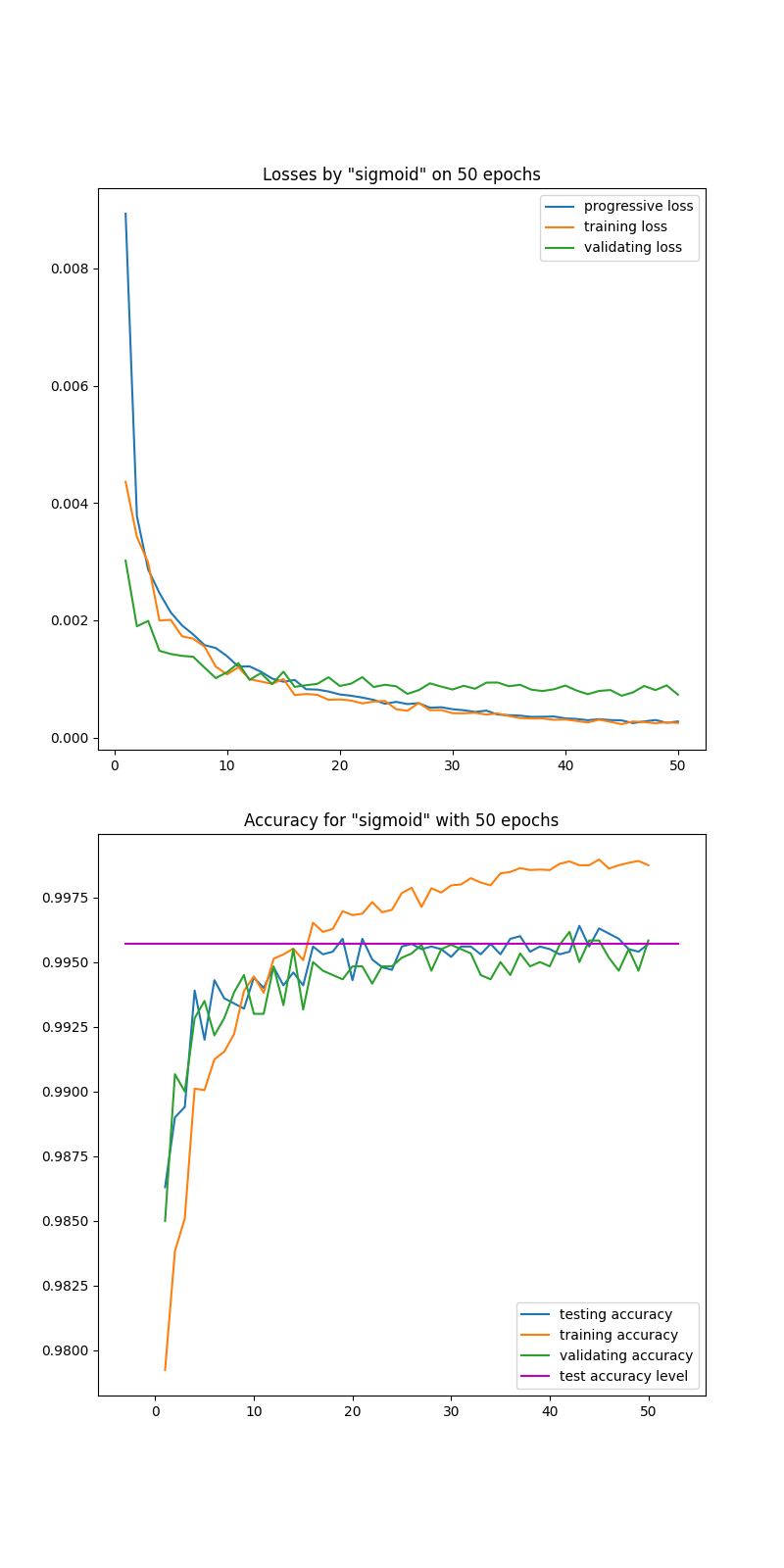
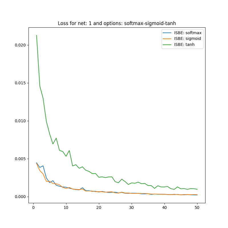
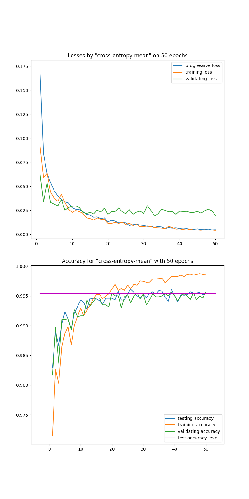
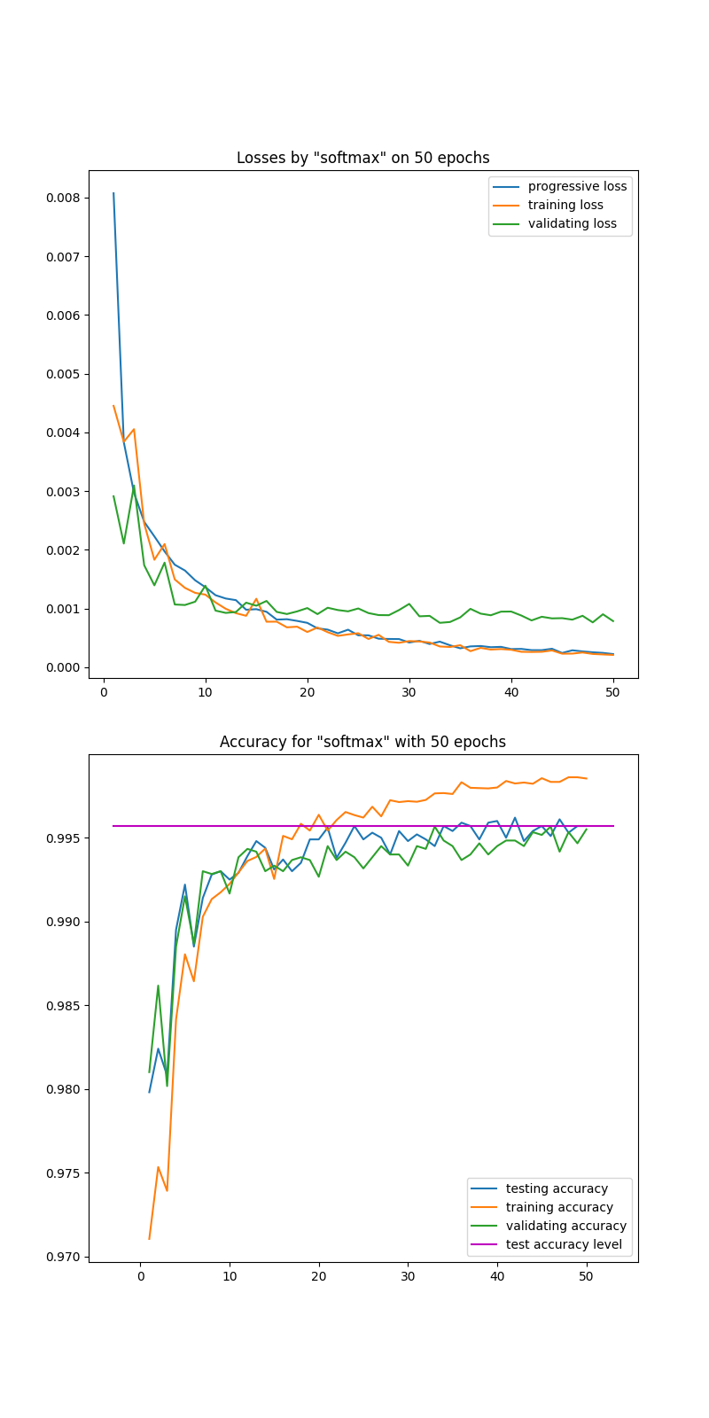
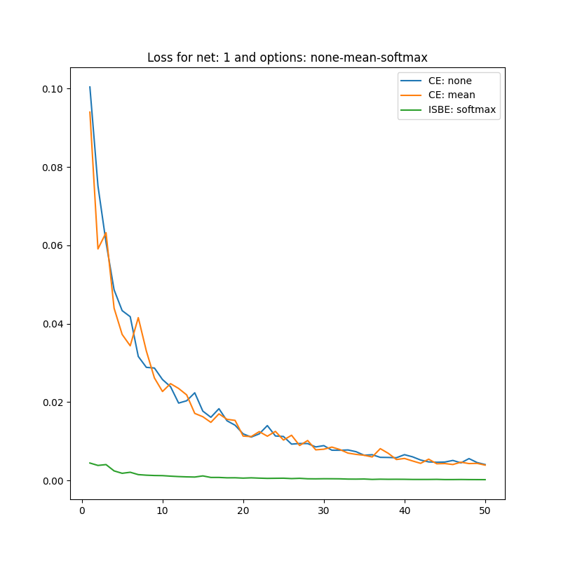
First, let’s see on three models cross-entropy-mean, softmax, sigmoid their loss and efficiency curves obtained on training data MNIST(54K) and on data intended solely for model validation MNIST(6K) . These two loss curves are calculated after each epoch. We supplement them with a loss curve calculated progressively after each batch of training data (see figure 1).

Let us note the correct course of the train loss curve with respect to progressive loss curve - both curves are close. The correct course is also for validation loss curve - the validation curve from about epoch 30 is below the training curve maintaining a significant distance. This is a sign that the model is not overfitted. This effect was achieved only after applying a moderate input image augmentation procedure.

Correct behavior of learning curves was recorded both for the modesl with entropy and for models with the ISBE unit. This also applies to classifier performance curves.

Figure 1: Learning curves on training and validation data for the $\mathcal{N}_{1}$ network and three models: cross-entropy-mean, softmax, sigmoid. The horizontal reference line represents the accuracy on test data computed after the last epoch.

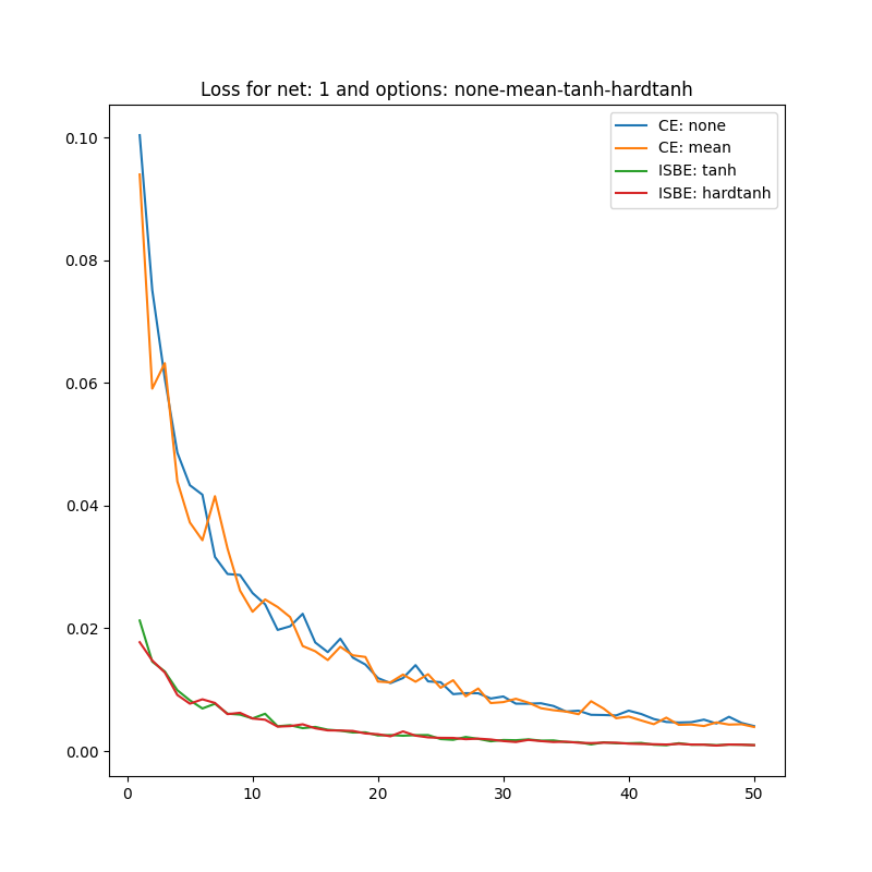
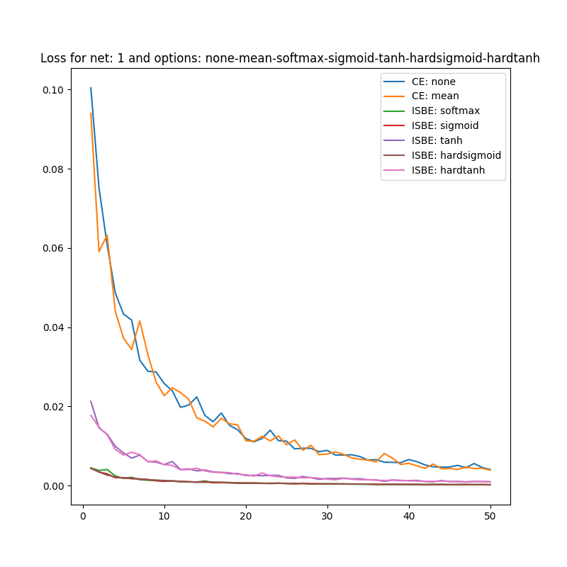
1. Curves of loss functions can appear together as long as the type of function is identical, which entails a similar range of variability for loss function values. One might wonder what measure of loss to adopt in the case of ISBE, since this technique, in fact, does not calculate loss values. We opt for a natural choice of mean square error for errors in soft scores:

   $$\mathcal{L}_{ISBE}=MSE(Y,Y^{\circ})\doteq\frac{1}{n_{b}}\cdot\|Y-Y^{\circ}\|^{2}_{2}$$

   For such defined measures, it turns out that only the option of reduction by summing has a different range of variability, and therefore it is not on the figure 2.

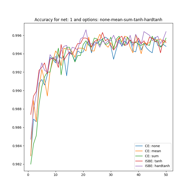
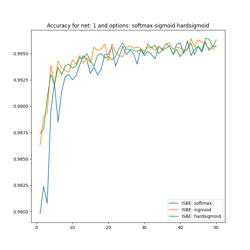
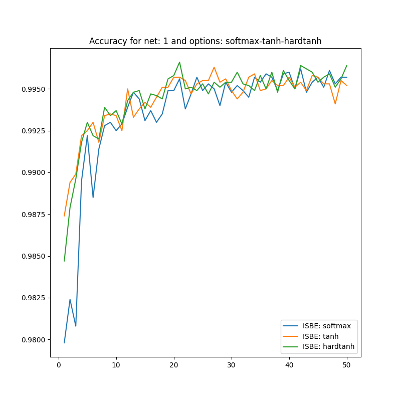
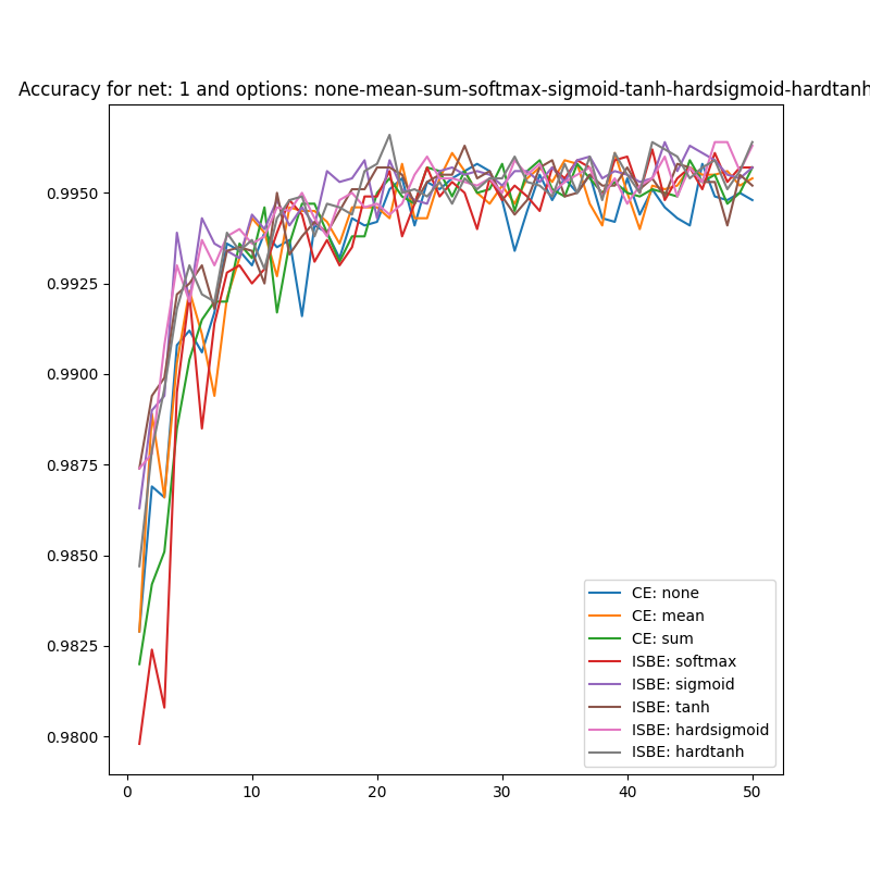
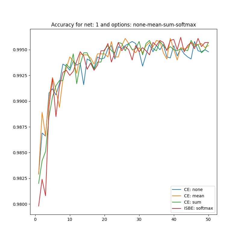
2. In the case of classifier accuracy, a common percentage scale does not exclude placing all eight curves for each considered architecture. However, due to the low transparency of such a figure, it is also worth juxtaposing different groups of curves of the dependency $\alpha(e)$. The accuracy $\alpha$ of the classifier MNIST(60K) is calculated on the test set MNIST(10K).

Sets of curves, which we visualize separately for architectures $\mathcal{N}_{0}$, $\mathcal{N}_{1}$ are:

• all options for loss functions (3) and soft score functions (5),

• CE none, CE mean, CE sum versus softmax,

• CE none, CE mean, CE sum versus tanh, hardtanh,

• softmax versus sigmoid, hardsigmoid,

• softmax versus tanh, hardtanh,

• softmax versus sigmoid, tanh.

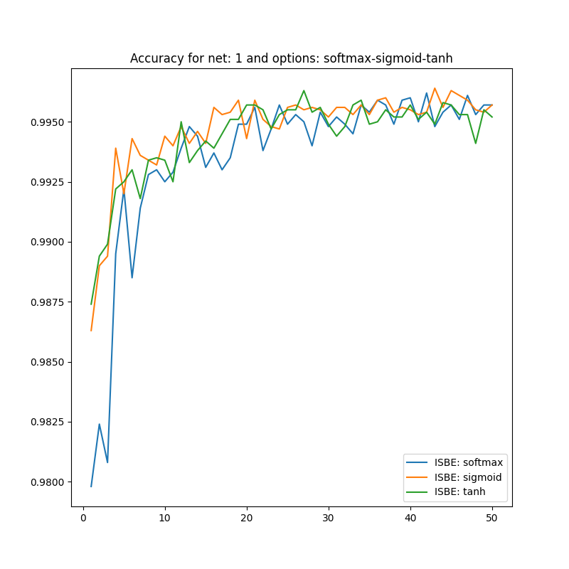
Due to space constraints, we show learning curves and classifier effectiveness graphs only for architecture $\mathcal{N}_{1}$ in figures 2, 3.

In figure 2 we can clearly observe four clusters of models:

• CrossEntropyLoss based with reduction option sum (as out of common range it was not shown),

• CrossEntropyLoss based with reduction options none, and mean,

• ISBE based with normalizations to range $[0,1]$ including functions
  $SoftMax,$ $Sigmoid,$ and $HardSigmoid$,

• ISBE based with normalizations to range $[-1,1]$ including functions $Tanh,$ and $HardTanh$.

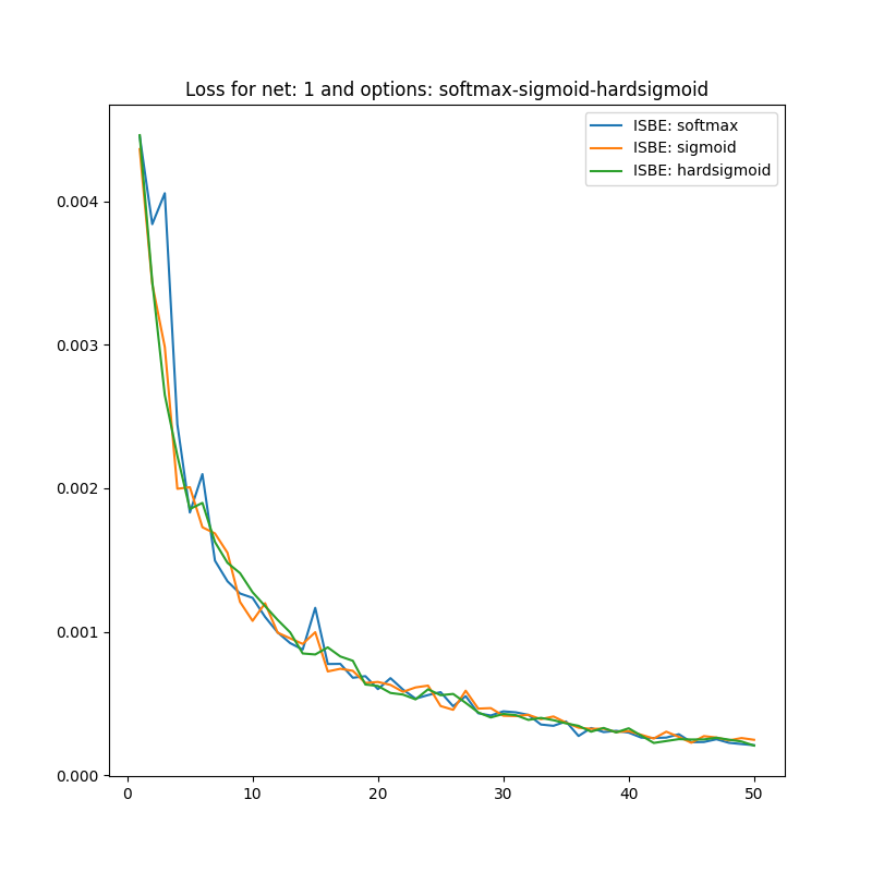
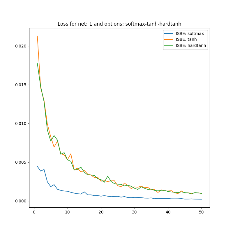
Within a cluster, the loss curves behave very similarly. Interestingly, the loss curves in ISBE-based clusters tend to the same value greater than zero. In contrast, cross-entropy-based curves also tend to the same limit. However it is clearly greater than ISBE one.

Figure 2: Loss charts of learning in comparisons of CE versus ISBE options. In the first row: (1) all options for loss functions and soft score functions; (2) CE none, CE mean versus softmax; (3): CE none, CE mean versus tanh, hardtanh. In the second row: (1) softmax versus sigmoid, hardsigmoid; (2) softmax versus tanh, hardtanh; (3) softmax versus sigmoid, tanh.

Now, we will pay more attention to test learning curves. We generate test learning curves on the full set of test data MNIST(10K). After each epoch, one point is scored towards the test learning curve. We will show these curves in several comparative contexts.

Figure 3: Accuracy charts of learning in comparisons of CE versus ISBE options. In the first row: (1) all options for loss functions and soft score functions; (2) CE none, CE mean versus softmax; (3): CE none, CE mean versus tanh, hardtanh. In the second row: (1) softmax versus sigmoid, hardsigmoid; (2) softmax versus tanh, hardtanh; (3) softmax versus sigmoid, tanh.

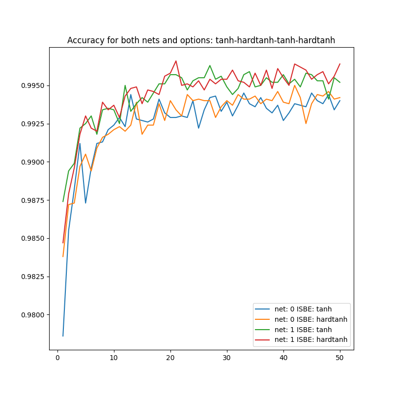
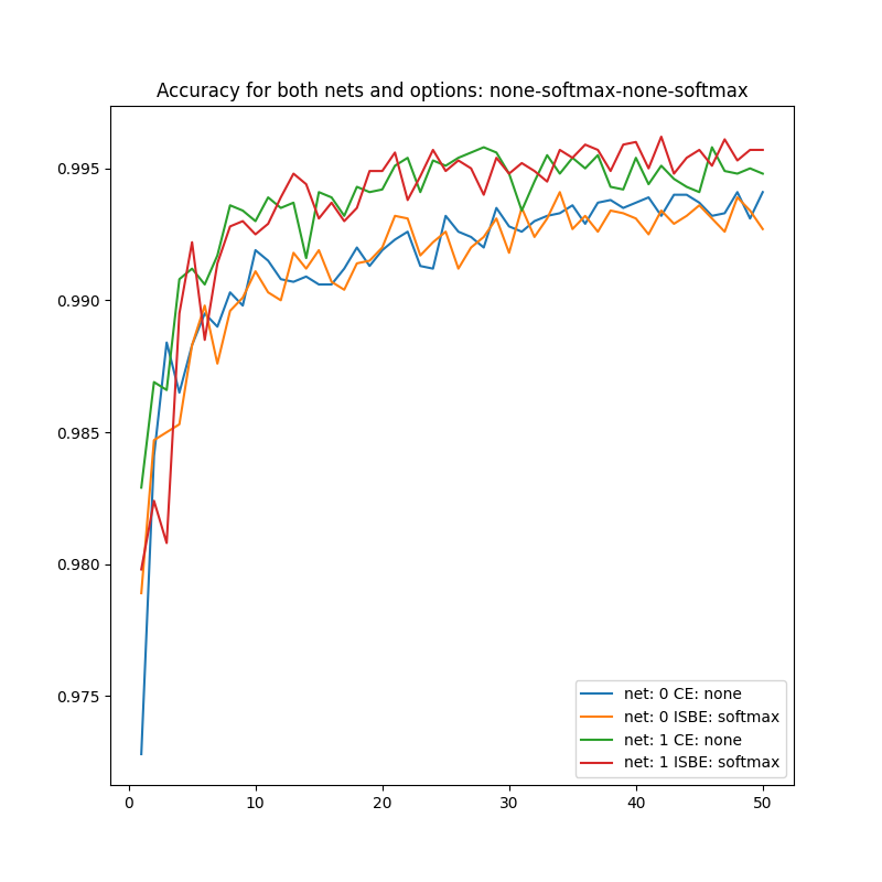
In the case of classifier accuracy curves (see figure 3), the variances in the clusters described above are smaller than in the union of clusters. Close to the final epochs, all curves tend to be chaotic within the range of $(99.4,99.7)$.

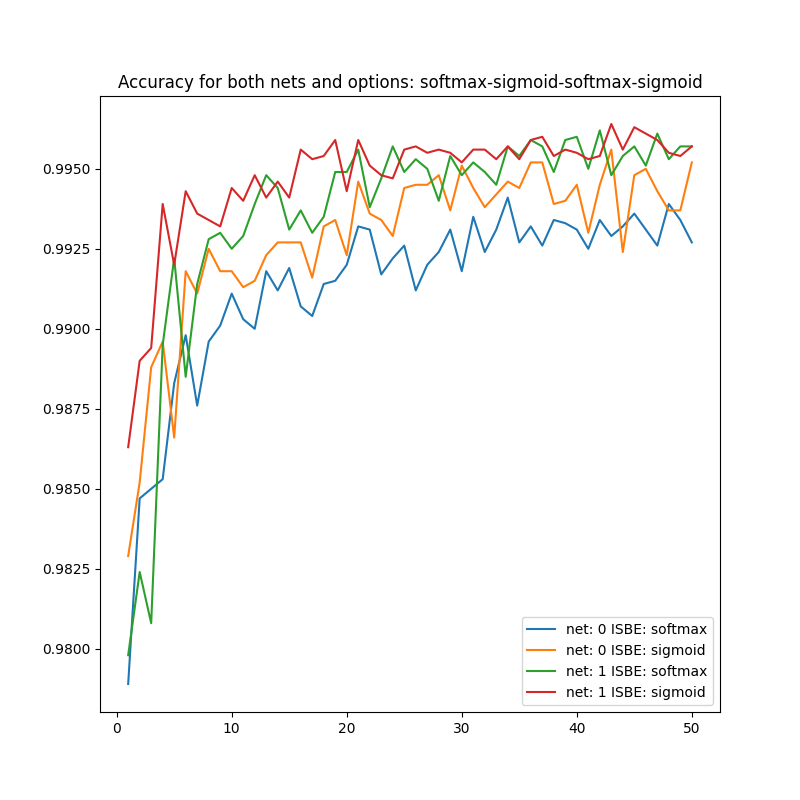
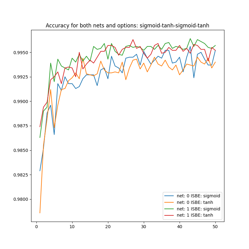
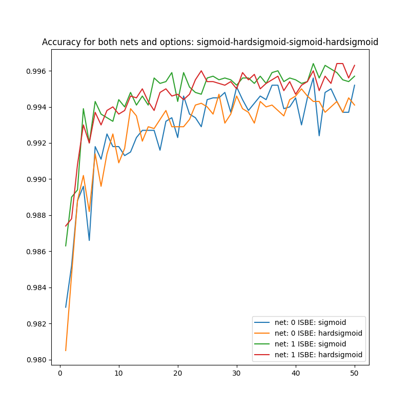
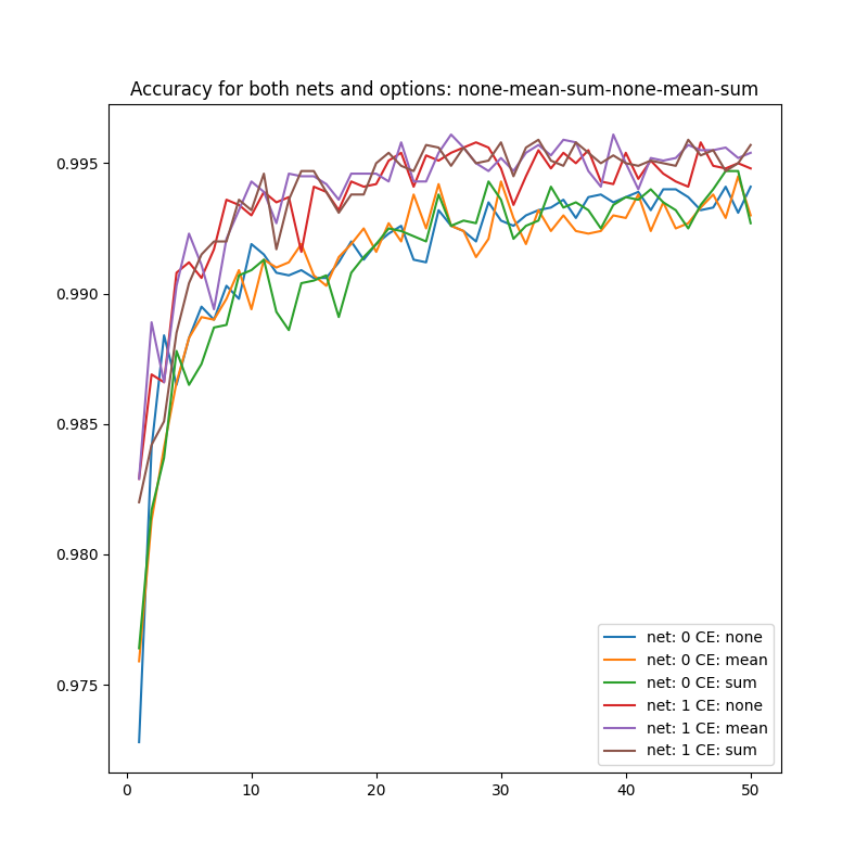
Visualizing the effectiveness of classifiers for different architectures of different complexities, although more obvious, also has research value (see figure 4):

• CE none, CE mean, CE sum from $\mathcal{N}_{0}$ versus CE none, CE mean, CE sum from $\mathcal{N}_{1}$,

• CE none, softmax from $\mathcal{N}_{0}$ versus CE none, softmax from $\mathcal{N}_{1}$,

• softmax, sigmoid from $\mathcal{N}_{0}$ versus softmax, sigmoid from $\mathcal{N}_{1}$,

• sigmoid, tanh from $\mathcal{N}_{0}$ versus sigmoid, tanh from $\mathcal{N}_{1}$,

• sigmoid, hardsigmoid from $\mathcal{N}_{0}$ versus sigmoid, hardsigmoid from $\mathcal{N}_{1}$,

• tanh, hardtanh from $\mathcal{N}_{0}$ versus tanh, hardtanh from $\mathcal{N}_{1}$.

The figure 4 shows the better performance of $\mathcal{N}_{1}$ than $\mathcal{N}_{0}$. Moreover, we can observe slightly more stable behaviour for ISBN-based curves than for cross-entropy-based.

Figure 4: Accuracy charts of learning in comparisons of CE versus ISBE options and architecture $\mathcal{N}_{0}$ versus $\mathcal{N}_{1}$. In the first row: (1) CE none, CE mean, CE sum; (2) CE none, softmax; (3): softmax, sigmoid. In the second row: (1) sigmoid, tanh; (2) sigmoid, hardsigmoid ; (3) tanh, hardtanh.

4 Conclusions

Cross-entropy CE as a loss function owes much to normalization performed by the SoftMax activation function. In the backward gradient backpropagation phase, only this activation, through perfect linearization, can prevent the explosion or suppression of the gradient originating from CE. What we call the softmax trick, as a mathematical phenomenon is explained by the theory presented in Appendix A. There is a proof that such linearization can only be realized by a function $F:\mathbb{R}^{K}\rightarrow\mathbb{R}^{K}$ with a Jacobian identical to that of the SoftMax function. In turn, such a Jacobian can only be by relocated versions of the SoftMax function.

For another research there are left practical aspects of more general theorem 2 implying that dilated and relocated versions of SoftMax, are the only ones having the property of dilated softmax trick.

Should we, therefore, celebrate this unique relationship between activation and cost function? In this work, I have shown that it is rather beneficial to use the final effect of the action of this pair, namely the linear value equal to $Y-Y^{\circ}$, which can be calculated without their participation. This is exactly what the ISBE unit does - it calculates the soft score vector in the forward step to return in backward step its error from the target score.

To determine the normalized score, the ISBE unit can use not only the SoftMax function, as it is not necessary to meet the unity condition, i.e., to ensure a probability distribution as scores of the trained classifier. At least four other activation functions Sigmoid, Tanh and their hard versions HardSigmoid and HardTanh perform no worse. The choice of these final activations was rather a matter of chance, so researchers face further questions. How to normalize raw scores and how to appropriately represent (encode) class labels in relation to this normalization, so as not to degrade the classifier’s results? What properties should such normalization functions have? Experiments suggest that meeting the Lipschitz condition in the vicinity of zero may be one of these properties.

The theoretical considerations presented prove that the ISBE unit in the process of deep model learning correctly simulates the behavior of the CrossEntropy unit preceded by the SoftMax normalization.

The experiments showed that the ISBE unit saves the time time of forward and backward stage up to $3\%$, and the effectiveness of the classifier model remains unchanged within the margin of statistical error.

On the other hand, the examples of code fragments showed that the programmer’s time spent on introducing the ISBE technique to his/her program instead of CrossEntropyLoss is negligible.

Appendix A Cross-Entropy and Softmax Trick Properties

The discrete cross-entropy function $CE$ of a target discrete probability distribution $y^{\circ}\in[0,1]^{K},\ \sum_{i}y^{\circ}_{i}=1$, relative to the distribution calculated by the classifier $y\in(0,1)^{K},\ \sum_{i}y_{i}=1$, is defined by the formula $CE(y^{\circ},y)\doteq-\sum_{i}y^{\circ}_{i}\ln y_{i}$.

The gradient of $CE$ with respect to $y$ is $\nabla_{y}CE(y^{\circ},y)=-y^{\circ}\div y,$ where the operation $w=u\div v$ denotes division by components of vectors $u,v$, i.e., $w_{i}\doteq u_{i}/v_{i}$, $i\in[K]$. The notation $[K]$ refers to a sequence of $K$ indices, such as $(1,\dots,K)$ or $(0,1,\dots,K-1)$.

In the special case when the vector $y\in(0,1)^{K}$ is calculated based on the vector $x\in\mathbb{R}^{K}$ according to the formula $y_{i}=SoftMax(x)_{i}=e^{x_{i}}/\sum_{k}e^{x_{k}}$, the gradient of $CE$ with respect to $x$ has a particularly simple resultant formula. Its simplicity was the reason for the term softmax trick:

$$y=SoftMax(x)\longrightarrow\nabla_{x}CE(y^{\circ},y(x))\overset{\text{\it softmax trick}}{=}y-y^{\circ}$$

Some authors ([29]) also use the term softmax trick for that part of the proof showing that the derivative of the natural logarithm of the sum of functions $e^{x_{i}}$ equals to the $SoftMax$ function:

$$\begin{array}[]{l}\displaystyle y_{i}\doteq\frac{e^{x_{i}}}{\sum_{k}e^{x_{k}}}\longrightarrow\displaystyle\frac{\partial{\left[\ln(\sum_{k}e^{x_{k}})\right]}}{\partial{x_{i}}}=y_{i}\longrightarrow\\[10.0pt] \begin{array}[]{rcl}\displaystyle\frac{\partial{CE(y^{\circ},y(x))}}{\partial{x_{i}}}&=&\displaystyle\frac{\partial{\left[\sum_{j}y^{\circ}_{j}\ln(\sum_{k}e^{x_{k}})-\sum_{j}y^{\circ}_{j}\ln e^{x_{j}}\right]}}{\partial{x_{i}}}\\ &=&y_{i}\overbrace{\sum_{j}y^{\circ}_{j}}^{=1}-y^{\circ}_{i}=y_{i}-y^{\circ}_{i}\quad\Box\end{array}\end{array}$$

In matrix notation ([30]), the property of softmax trick has a longer proof, as we first need to calculate the Jacobian of the $SoftMax$ function ([31]), which is $\frac{\partial{y}}{\partial{x}}=\mathtt{diag}\left[y\right]-y{y}^{\intercal}$. Then

$$\begin{array}[]{rcl}\displaystyle\frac{\partial{[CE(y^{\circ},y(x))]}}{\partial{x}}&=&\displaystyle\frac{\partial{y}}{\partial{x}}\cdot\nabla_{y}CE(y^{\circ},y)=\left(\mathtt{diag}\left[y\right]-y{y}^{\intercal}\right)\left(-y^{\circ}\div y\right)\\[8.0pt] &=&\displaystyle y\underbrace{{(y\div y)}^{\intercal}y^{\circ}}_{{\mathbf{1}}^{\intercal}_{K}y^{\circ}=1}-\underbrace{\mathtt{diag}\left[y\div y\right]}_{I_{K}}y^{\circ}=y-y^{\circ}\end{array}$$

An interesting question arises: Is it only the $SoftMax$ function that has such a property? It seems possible, as for any differentiable function $F:\mathbb{R}^{n}\rightarrow\mathbb{R}^{n}$ the starting point is similar:

$$\frac{\partial{\left[CE(y^{\circ},\underbrace{F(x)}_{y})\right]}}{\partial{x}}=\frac{\partial{F(x)}}{\partial{x}}\overbrace{\frac{\partial{[CE(y^{\circ},y)]}}{\partial{y}}}^{-y^{\circ}\div y}=\frac{\partial{F(x)}}{\partial{x}}(-y^{\circ}\div y)$$

The following theorem fully characterizes functions that have the softmax trick property.

Theorem 1 (on the properties of softmax trick).

For a differentiable function $F:\mathbb{R}^{K}\rightarrow\mathbb{R}^{K}$, the following three properties are equivalent:

1. $F$ is a SoftMax function with relocation, if there exists a reference point $c\in\mathbb{R}^{K}$, such that for every $x\in\mathbb{R}^{K}$:

   $$y=F(x)=SoftMax(x-c)\,,$$

2. $F$ has a softmax-type Jacobian, if for every $x\in\mathbb{R}^{K}$:

   (5) $$Jacobian(F)(x)\doteq\frac{\partial{F(x)}}{\partial{x}}=\mathtt{diag}\left[y\right]-y{y}^{\intercal}\,,\text{ where }y=F(x)\,,$$

3. $F$ possesses the softmax trick property, if for every $y^{\circ}\in[0,1]^{K},x\in(0,1)^{K}$:

   (6) $$\frac{\partial{F(x)}}{\partial{x}}(-y^{\circ}\div y)=y-y^{\circ}\,,\text{ where }y=F(x)\,.$$

Proof of Theorem 1.

We prove the implications in the following order: $(2)\longrightarrow(3),\ (3)\longrightarrow(2)$,  $(1)\longrightarrow(2),\ (2)\longrightarrow(1)\,.$

• Proof of implication $(2)\longrightarrow(3)$:

  If the Jacobian $\frac{\partial{F(x)}}{\partial{x}}$ of the function $F$ is of the softmax type, then for $y=F(x)$:

  $$\frac{\partial{y}}{\partial{x}}=\left(\mathtt{diag}\left[y\right]-y{y}^{\intercal}\right)\left(-y^{\circ}\div y\right)=y\underbrace{{(y\div y)}^{\intercal}y^{\circ}}_{{\mathbf{1}}^{\intercal}_{K}y^{\circ}=1}-\underbrace{\mathtt{diag}\left[y\div y\right]}_{I_{K}}y^{\circ}=y-y^{\circ}\quad\Box$$

• Proof of implication $(3)\longrightarrow(2)$: Denote the axis unit vector $j$ by $e_{j}\in\mathbb{R}^{K}$. Then $(e_{j})_{i}=\delta_{ij}$. Substitute into property (6) the target score vector $y^{\circ}\doteq e_{j}$. Then

  $$y_{i}-(e_{j})_{i}={\left(\frac{\partial{F(x)}}{\partial{x_{i}}}\right)}^{\intercal}(-e_{j}\div y)=\sum_{k\in[K]}\frac{\partial{y_{k}}}{\partial{x_{i}}}\cdot\left(\frac{-\delta_{kj}}{y_{k}}\right)=\frac{\partial{y_{j}}}{\partial{x_{i}}}\cdot\left(\frac{-1}{y_{j}}\right)$$

  Therefore $\frac{\partial{y_{j}}}{\partial{x_{i}}}=((e_{j})_{i}-y_{i})y_{j}\overset{(e_{j})_{i}=\delta_{ij}}{=}(\delta_{ij}-y_{i})y_{j}$. Thus, $\frac{\partial{y}}{\partial{x}}=\mathtt{diag}\left[y\right]-y{y}^{\intercal}\,.$ $\Box$

• Proof of implication $(1)\longrightarrow(2)$:

  If $\displaystyle y_{j}\doteq\frac{e^{x_{j}-c_{j}}}{\sum_{k\in[K]}e^{x_{k}-c_{k}}}$, then
  $\displaystyle\frac{\partial{y_{j}}}{\partial{x_{i}}}=\left\{\begin{array}[]{l}\displaystyle\frac{-e^{x_{j}-c_{j}}\cdot e^{x_{i}-c_{i}}}{\left(\sum_{k\in[K]}e^{x_{k}-c_{k}}\right)^{2}}=-y_{i}\cdot y_{j},\ \text{when }i\neq j\\[20.0pt] \displaystyle\frac{e^{x_{i}-c_{i}}\cdot\left(\sum_{k\in[K]}e^{x_{k}-c_{k}}\right)-e^{x_{i}-c_{i}}\cdot e^{x_{i}-c_{i}}}{\left(\sum_{k\in[K]}e^{x_{k}-c_{k}}\right)^{2}}\\[20.0pt] =y_{i}-y_{i}^{2}=(1-y_{i})\cdot y_{i},\ \text{when }i=j\end{array}\right.$

  The general formula is $\displaystyle\frac{\partial{y_{j}}}{\partial{x_{i}}}=(\delta_{ij}-y_{i})y_{j}\,.$ Therefore:

  $$\left(\frac{\partial{y}}{\partial{x}}\right)_{ij}\doteq\frac{\partial{y_{j}}}{\partial{x_{i}}}=\delta_{ij}y_{j}-y_{i}y_{j}=\left(\mathtt{diag}\left[y\right]\right)_{ij}-\left(y{y}^{\intercal}\right)_{ij}\,.$$

  Hence, $\frac{\partial{y}}{\partial{x}}=\mathtt{diag}\left[y\right]-y{y}^{\intercal}\quad\Box$

• Proof of implication $(2)\longrightarrow(1)$:
  If $\frac{\partial{y_{i}}}{\partial{x_{i}}}=(1-y_{i})\cdot y_{i}$, then the diagonal of the Jacobian matrix gives us differential equations ([32]), from which we can determine the general form of the function $y_{i}(x)$, $i\in[K]:$

  $$\begin{array}[]{l}\displaystyle\frac{\partial y_{i}}{(1-y_{i})\cdot y_{i}}=\partial x_{i}\longrightarrow\int\left(\displaystyle\frac{1}{y_{i}}+\frac{1}{1-y_{i}}\right)\partial y_{i}=\int\partial x_{i}\\[15.0pt] \displaystyle\longrightarrow\ln\frac{y_{i}}{1-y_{i}}=x_{i}+C(k\neq i)\longrightarrow\displaystyle y_{i}=\displaystyle\frac{e^{x_{i}}}{\underbrace{e^{x_{i}}+e^{-C(k\neq i)}}_{z_{i}}}\\[10.0pt] \longrightarrow\displaystyle y_{i}=\frac{e^{x_{i}}}{z_{i}},\text{ where }z_{i}=z_{i}(x_{1},\dots,x_{K})>0\\[10.0pt] \longrightarrow\ln{z_{i}}=x_{i}-\ln y_{i}\end{array}$$

  Now we calculate the partial derivatives $\frac{\partial{\ln z_{j}}}{\partial{x_{i}}}$. If $i\neq j$, then

  $$\frac{\partial{[\ln z_{j}]}}{\partial{x_{i}}}=\frac{\partial{[x_{j}-\ln y_{j}]}}{\partial{x_{i}}}=-\frac{1}{y_{j}}\overbrace{\frac{\partial{y_{j}}}{\partial{x_{i}}}}^{-y_{j}y_{i}}=y_{i}$$

  For $i=j$, the result is the same:

  $$\frac{\partial{[\ln z_{i}]}}{\partial{x_{i}}}=\frac{\partial{[x_{i}-\ln y_{i}]}}{\partial{x_{i}}}=1-\frac{1}{y_{i}}\overbrace{\frac{\partial{y_{i}}}{\partial{x_{i}}}}^{(1-y_{i})y_{i}}=1-\frac{(1-y_{i})y_{i}}{y_{i}}=y_{i}$$

  Therefore, for a fixed $i$, e.g., for $j=1$, we have $K$ equalities: $\frac{\partial{[\ln z_{1}]}}{\partial{x_{i}}}=\frac{\partial{[\ln z_{j}]}}{\partial{x_{i}}}=y_{i}$ for any $j,i\in[K]$. This means that vector fields for each pair of functions $\ln z_{1}$ and $\ln z_{j}$ are identical.

  Integrating these fields yields the same functions up to a constant $c_{j}$: $\ln z_{j}=\ln z_{1}+c_{j},$ $j\in[K]$. Consequently, $z_{j}=z_{1}\cdot e^{c_{j}}$, $j\in[K]$, and therefore $y_{j}=\displaystyle\frac{e^{x_{j}}}{z_{1}e^{c_{j}}}=\frac{e^{x_{j}-c_{j}}}{z_{1}}$. From the unity condition, we can now determine the value of $z_{1}$:

  $$1=\sum_{k\in[K]}y_{k}=\sum_{k\in[K]}\frac{e^{x_{k}-c_{k}}}{z_{1}}\longrightarrow z_{1}=\sum_{k\in[K]}e^{x_{k}-c_{k}}\longrightarrow y_{j}=\displaystyle\frac{e^{x_{j}-c_{j}}}{\displaystyle\sum_{k\in[K]}e^{x_{k}-c_{k}}}\,.$$

∎

The theorem 1 can be generalized to dilated version of the SoftMax function. It is reformulated in the form of theorem 2. The proof of the generalized theorem can be easily generalized, too.

Theorem 2 (on the properties of dilated softmax trick).

For a differentiable function $F:\mathbb{R}^{K}\rightarrow\mathbb{R}^{K}$, the following three properties are equivalent:

1. $F$ is a SoftMax function with dilation and relocation, if there exists a reference point $c\in\mathbb{R}^{K}$, and dilation vector $d\in\mathbb{R}^{K}$, $\forall i,d_{i}\neq 0$ such that for every $x\in\mathbb{R}^{K}$:

   $$y=F(x)=SoftMax(d\odot x-c)\,,$$

2. $F$ has a dilated softmax-type Jacobian, if there exists a dilation vector $d\in\mathbb{R}^{K}$ such that for every $x\in\mathbb{R}^{K}$:

   $$Jacobian(F)(x)\doteq\frac{\partial{F(x)}}{\partial{x}}=d\odot\left(\mathtt{diag}\left[y\right]-y{y}^{\intercal}\right)\,,\text{ where }y=F(x)\,,$$

3. $F$ possesses the dilated softmax trick property, if there exists a dilation vector $d\in\mathbb{R}^{K}$ such that for every $y^{\circ}\in[0,1]^{K},x\in(0,1)^{K}$:

   $$\frac{\partial{F(x)}}{\partial{x}}(-y^{\circ}\div y)=d\odot(y-y^{\circ})\,,\text{ where }y=F(x)\,.$$

References

• [1] Schmidhuber J. Annotated History of Modern AI and Deep Learning. arXiv:2212.11279, 2022.
• [2] Rosenblatt F. The Perceptron: A Probabilistic Model For Information Storage And Organization in the Brain. Psychological Review. 65 (6): 386–408, 1958.
• [3] Amari S.I. A theory of adaptive pattern classifier. IEEE Trans, EC-16, 279-307, 1967.
• [4] Golden R.M. Mathematical Methods for Neural Network Analysis and Design. The MIT Press, 1996.
• [5] Fergus P., Chalmers C. Applied Deep Learning - Tools, Techniques, and Implementation. Springer Cham, Springer Nature Switzerland, 2022.
• [6] Hinton G. How to Represent Part-Whole Hierarchies in a Neural Network. Neural Computation 35 (3): 413–452, 2023.
• [7] MacKay D.J.C. Information Theory, Inference, and Learning Algorithms. Cambridge University Press, 2003.
• [8] Kingma D.P., Ba J. Adam: A Method for Stochastic Optimization. arXiv:1412.6980, 2014.
• [9] Werbos P. J. Applications of advances in: nonlinear sensitivity analysis. in: Drenick R., Kozin: F. (eds): System Modeling and Optimization: Proc. IFIP, Springer, 1982.
• [10] Rumelhart D.E., Hinton G.E., Williams R.J. Learning Representations by Back-propagating Errors. in: Neurocomputing: Foundations of Research, MIT Press, 1988.
• [11] Paszke A., et al. Automatic differentiation in: PyTorch. 31st Conference on Neural Information Processing Systems NIPS, 2017.
• [12] Lecun Y., Bottou L., Bengio Y. , Haffner P. Gradient-based learning applied to document recognition. in: Proceedings of the IEEE, vol. 86, no. 11, pp. 2278-2324, 1998.
• [13] Sahin: H.M., Miftahushudur T., Grieve B., Yin: H.. Segmentation of weeds and crops using multispectral imaging and CRF-enhanced U-Net. Computers and Electronics in: Agriculture, Volume 211, 2023.
• [14] Yan G., Jing H., Li H., Guo H., He S. Enhancing Building Segmentation in: Remote Sensing Images: Advanced Multi-Scale Boundary Refinement with MBR-HRNet. Remote Sensing, 2023.
• [15] Min: B., et alt. Recent Advances in: Natural Language Processing via Large Pre-Trained Language Models: A Survey. ArXiv:2111.01243, 2021.
• [16] Majumdar S., Ginsburg B. MatchboxNet: 1D Time-Channel Separable Convolutional Neural Network Architecture for Speech Commands Recognition. ArXiv:2004.08531v2, 2020.
• [17] Chung J.S., Nagrani A., Zisserman, A. VoxCeleb2: Deep Speaker Recognition. INTERSPEECH, 2018.
• [18] Han J., et alt. DiaCorrect: Error Correction Back-end For Speaker Diarization. arXiv:2309.08377, 2023.
• [19] Chang X., Skarbek W. Multi-Modal Residual Perceptron Network for Audio–Video Emotion Recognition. Sensors 21(16), 2021.
• [20] Reis D., et alt. Real-Time Flying Object Detection with YOLOv8. ArXiv:2305.09972, 2023.
• [21] Bridle J.S. Probabilistic Interpretation of Feedforward Classification Network Outputs, with Relationships to Statistical Pattern Recognition. in: Soulié, F.F., Hérault, J. (eds) Neurocomputing. NATO ASI Series, vol 68. Springer, Berlin, Heidelberg: Springer. pp. 227–236, 1990.
• [22] Bishop C.M. Pattern Recognition and Machine Learning. Springer, 2006.
• [23] Mohri M., Rostazadeh A., Talwalkar A. Foundations of Machine Learning. The MIT Press, 2012.
• [24] Cho J.H., Hariharan B. On the Efficacy of Knowledge Distillation. ArXiv: 1910.01348, 2019.
• [25] Anonymous Blogger. (accessed on 11.11.2023). Softmax classification with cross-entropy. link: https://peterroelants.github.io/posts/cross-entropy-softmax/
• [26] LeCun Y., et alt. (accessed on 11.11.2023). THE MNIST DATABASE of handwritten digits. link: http://yann.lecun.com/exdb/mnist/, 1998
• [27] Gao B., Lacra P. On the Properties of the Softmax Function with Application in: Game Theory and Reinforcement Learning arXiv:1704.00805, 2018.
• [28] Skarbek W. Symbolic Tensor Neural Networks for Digital Media – from Tensor Processing via BNF Graph Rules to CREAMS Applications. Fundamenta Informaticae, vol. 168, no. 2-4, pp. 89-184, 2019.
• [29] Bendersky E. (accessed on 11.11.2023). The Softmax function and its derivative. link: https://eli.thegreenplace.net/2016/the-softmax-function-and-its-derivative/
• [30] Golub G.H., Van Loan C.F. Matrix Computations. Johns Hopkins University Press, 3rd edition, 1996.
• [31] Liu S. et alt. Matrix differential calculus with applications in: the multivariate linear model and its diagnostics. Journal of Multivariate Analysis, 188, 2022.
• [32] Riley K.F., Hobson M.P., Bence S.J. Mathematical methods for physics and engineering. Cambridge University Press, 2010.