Abstract

Physical and functional constraints on biological networks lead to complex topological patterns across multiple scales in their organization. A particular type of higher-order network feature that has received considerable interest is network motifs, defined as statistically regular subgraphs. These may implement fundamental logical and computational circuits and are referred as “building blocks of complex networks”. Their well-defined structures and small sizes also enables the testing of their functions in synthetic and natural biological experiments. The statistical inference of network motifs is however fraught with difficulties, from defining and sampling the right null model to accounting for the large number of possible motifs and their potential correlations in statistical testing. Here we develop a framework for motif mining based on lossless network compression using subgraph contractions. The minimum description length principle allows us to select the most significant set of motifs as well as other prominent network features in terms of their combined compression of the network. The approach inherently accounts for multiple testing and correlations between subgraphs and does not rely on a priori specification of an appropriate null model. This provides an alternative definition of motif significance which guarantees more robust statistical inference. Our approach overcomes the common problems in classic testing-based motif analysis. We apply our methodology to perform comparative connectomics by evaluating the compressibility and the circuit motifs of a range of synaptic-resolution neural connectomes.

Author summary

Networks provide a useful abstraction to study complex systems by focusing on the interplay of the units composing a system rather than on their individual function. Network theory has proven particularly powerful for unraveling how the structure of connections in biological networks influence the way they may process and relay information in a variety of systems ranging from the microscopic scale of biochemical processes in cells to the macroscopic scales of social and ecological networks. Of particular interest are small stereotyped circuits in such networks, termed motifs, which may correspond to building blocks implementing fundamental operations, e.g., logic gates or filters. We here present a new tool that finds sets of motifs in networks based on an information-theoretic measure of how much they allow to compress the network. This approach allows us to evaluate the collective significance of sets of motifs, as opposed to only individual motifs, and it does not require us to know the right null model to compare against beforehand, rather it infers it from the data. We apply our methodology to compare the neural wiring diagrams, termed “connectomes”, of the tadpole larva Ciona intestinalis and the ragworm Platynereis dumerelii, the nematode Caenorhabditis elegans and the fruitfly Drosophila melanogaster at different developmental stages.

Introduction

Network theory has highlighted remarkable topological features of many biological and social networks [1, 2, 3]. Some of the main ones are the small world property [4, 5, 6, 7], which refers to a simultaneous high local clustering of connections and short global distances between nodes; scale-free features, most notably witnessed by a broad distribution of node degrees [8, 9, 10, 11]; mesoscopic, and in particular modular, structuring [12, 13, 14]; and higher-order topological features [15], such as a statistical overrepresentation of certain types of subgraphs, termed network motifs [16, 17, 18].

We here focus on network motifs. They were first introduced to study local structures in social networks [19, 20, 21]. In biological networks, they are hypothesized to capture functional subunits (e.g., logic gates or filters) and have been extensively studied in systems ranging from transcription and protein networks to brain and ecological networks [16, 22, 17, 23, 24, 18, 2]. In contrast to most other remarkable features of biological networks, the well-defined structure and small size of network motifs mean that their function may be probed experimentally, both in natural [25, 26] and in synthetic experiments [25].

The prevailing approach to network motif inference involves counting or estimating the frequency of each subgraph type, termed a graphlet [27], and comparing it to its frequency in random networks generated by a null model [16, 28]. Subgraphs that appear significantly more frequently in the empirical network than in the random networks are deemed motifs. While this procedure has offered valuable insights, it also suffers from several fundamental technical complications which can make it statistically unreliable. First, motifs are inferred based either on a $Z$-test or on direct estimation of $p$ values from sampling of random networks. The former approach assumes Gaussian statistics under the null, which is often not a good approximation [29]. In the latter approach, it is only possible to evaluate $p$-values that are larger than $1/M$ where $M$ is the number of random networks analyzed. This is computationally expensive and precludes the evaluation of low $p$ values, which in turn makes it practically impossible to correct for multiple testing using standard approaches, such as the Bonferroni correction, which effectively decreases the significance threshold by a factor of the order of the number of tests. Second, the appropriate null model is often not known [30, 31, 32] or it may be computationally unfeasible to sample it [33, 31, 32]. However, results may crucially depend on the choice of null model, [30, 31], potentially leading to the inference of spurious motifs. Third, the frequencies of different graphlets are not guaranteed to be independent, so one should account for these correlations when performing statistical testing [29]. Moreover, one should also account for these correlations in the null model to avoid inferring spurious motifs [16, 34].

A principled manner to account for both multiple testing and correlations between graphlets is to build generative network models. Exponential random graph models (ERGMs) in principle provide such a family of generative models [35, 36]. However, in practice, they are hard to fit due to near-degeneracy [37, 36], so to ensure convergence of model fits one must in general resort to highly constrained motif choices only [34, 38, 39].

Information theory tells us that the presence of statistical regularities in a network makes it compressible [40]. Inspired by this fact, we here propose a methodology based on lossless compression [41] as a measure of significance and which implicitly defines a generative model through the correspondence between universal codes and probability distributions [40, 42]. We demonstrate how this approach allows to address the shortcomings of testing-based motif inference. First, it naturally lets us account for multiple testing and correlations between different motifs. Furthermore, since our approach is not based on random graph sampling, we can furthermore evaluate and compare even highly significant motifs. Finally, through the minimum description length (MDL) principle [42, 43], we can select not only the most significant motif configuration, but also other significant node- and link-level features such as node degrees and link reciprocity. This means that we do not need to define the null model beforehand as in testing-based approaches since we can instead infer the best fitting base description a posteriori.

We apply our methodology to discover microcircuit motifs in synapse resolution neuron wiring diagrams, the connectomes, of small animals which have recently become available thanks to advances in electron microscopy techniques and image segmentation [44, 45, 46, 47]. We compare the compressibility induced by motif sets and other network features found in different brain regions of different animals and at different developmental stages. We namely analyze the complete connectome of Caenorhabditis  elegans at different developmental stages, and the connectomes of different brain regions of both larval and adult Drosophila melanogaster, in addition to the complete connectomes of Platynereis dumerelii and larval Ciona intestinalis. We find that all the connectomes are compressible, implying significant non-random structure. We find that the compressibility varies between connectomes, with larger connectomes generally being more compressible. We infer motif sets in the majority of the connectomes, but we do not find significant evidence for motifs in the smallest connectomes. The typical motifs, which are found with high frequency in the different connectomes, tend to be dense subgraphs. We compare several topological measures of the motif sets, which show high similarity between connectomes, although with some significant differences.

Materials and methods

Graphlets and motifs

Network motif analysis is concerned with the discovery of statistically significant classes of subgraphs in empirically recorded graphs. We here restrict ourselves to directed unweighted graphs, but the concepts apply similarly to undirected networks and may even be extended to weighted [48, 49], time-evolving, and multilayer graphs [50, 51, 52, 53], and to hypergraphs [54, 55]. As is usual in motif analysis, we restrict ourselves to weakly connected subgraphs [16, 25]. This ensures that the subgraph may represent a functional subunit where all nodes can participate in information processing.

Let $G=(\mathcal{N},\mathcal{E})$ denote the directed graph we want to analyze. For simplicity in comparing different representations of $G$, we consider $G$ to be node-labeled. Thus, the nodes $\mathcal{N}=(1,2,\ldots,N)$ constitute an ordered set. The set of edges, $\mathcal{E}\subseteq\mathcal{N}\times\mathcal{N}$ indicates how the nodes are connected; by convention, a link $(i,j)\in\mathcal{E}$ indicates that $i$ connects to $j$. Note that since $G$ is directed, the presence of $(i,j)\in\mathcal{E}$ does not imply the existence of $(j,i)\in\mathcal{E}$.

An induced subgraph $g=({\nu},{\epsilon})$ of $G$ is the graph formed by a given subset ${\nu}\in\mathcal{N}$ of the nodes of $G$ and all the edges ${\epsilon}=\{(i,j):i,j\in{\nu}\land(i,j)\in\mathcal{E}\}$ connecting these nodes in $G$.

An undirected graph $G_{\rm un}$ is called connected if there exists a path between all pairs of nodes in $G_{\rm un}$. A directed graph $G$ is weakly connected if the undirected graph obtained by replacing all the directed edges in $G$ by undirected ones is connected.

Two graphs $g=({\nu},{\epsilon})$ and $g^{\prime}=({\nu}^{\prime},{\epsilon}^{\prime})$ are isomorphic if there exists a permutation $\sigma$ of the node indices of $g^{\prime}$ such that the edges in the graphs perfectly overlap, i.e., such that $(i,j)\in{\epsilon}$ if and only if $(\sigma(i),\sigma(j))\in{\epsilon}^{\prime}$. A graphlet, denoted by $\alpha$, is an isomorphism class of weakly connected, induced subgraphs [27], i.e., the set $\alpha=\{g:g\cong g_{\alpha}\}$ of all graphs that are isomorphic to a given graph, $g_{\alpha}$.

Finally, a motif is a graphlet that is statistically significant. Traditionally, a significant graphlet is defined as one whose number of occurrences in $G$ is significantly higher than in random graphs generated by a given null model [16]. Instead, we propose a method that selects a set of graphlets, $\Gamma=\{\alpha\}$, based on how well it allows to compress $G$. This allows to treat motif mining as a model selection problem through the MDL principle.

Subgraph census

The first part of a motif inference procedure is to perform a subgraph census, consisting in counting the occurrences of the graphlets of interest in $G$. Subgraph census is computationally hard and many methods have been developed to tackle it [56].

For graphs with a small number of nodes, i.e., hundreds of nodes, we implemented the parallelized FaSe algorithm [57] to perform the subgraph census, while for larger graphs, i.e., comprising a thousand nodes or more, we rely on its stochastic version, Rand-FaSe [58]. The algorithms use Wernicke’s ESU method (or Rand-ESU for large graphs) [59] for counting subgraph occurrences in $G$ and employ a trie data structure, termed g-trie [60], to store the graphlets and their occurrences in order to minimize the number of computationally costly subgraph isomorphism checks.

Since our algorithm relies on contracting individual subgraphs we also need to store the location of each subgraph in $G$. Due to the large number of subgraphs, the space required to store this information may exceed working memory for larger graphs or graphlets. Our most computationally challenging case (the right mushroom body of the adult Drosophila connectome), for example requires storing 1.3 TB of data. We write heavy textfiles of subgraph lists, one per graphlet, on the computer node static memory. Subgraphs can be retrieved through a random-access iterator through a collection of textfile pointers; hence the working memory gain is at least of the order of the subgraph size. When the pointer collection is still too large to be fully stored dynamically, an option allows reading subgraph lists by chunks of a controlled size (see Supplementary Note S1).

All scripts were run on the HPC cluster of the Pasteur Institute and can be found at https://gitlab.pasteur.fr/sincobe/brain-motifs.

Compression, model selection, and hypothesis testing

The massive number of possible graphlet combinations and the correlations between graphlet counts within a network make classic hypothesis-testing-based approaches for motif mining ill-suited for discovering motif sets. Additionally, classical methods define motif significance by comparison with a random graph null model, and the results may depend on the choice of null model [30, 31] (see “Numerical validation” in the results below). In the context of motif mining, the choice of null model can lead to ambiguities [30, 31, 32], thus rendering the analysis unreliable.

To address these problems, we cast motif mining as a model selection problem. We wish to select as motifs the multiset of graphlets, $\mathcal{S}^{*}=[\alpha^{*}]$ that, together with a tractable dyadic graph model, provides the best model for $G$. The minimum description length principle [42] states that, within an inductive inference framework with finite data, the best model is the one that leads to the highest compression, or minimum codelength, of the data. It relies on an equivalence between codelengths and probabilities [40] and formalizes the well-known Occam’s razor, or principle of parsimony. It is similar to Bayesian model selection and can be seen as a generalization of it [43].

To each dataset, model and parameter value, we associate a code, i.e., a label that identifies one representation. The code should be lossless, which means full reconstruction of the data from the compressed representation is possible [42, 40].

In practice, we are not interested in finding an actual code, but only in calculating the codelength of a universal code, e.g., the Shannon-Fano code [40], corresponding to our model.

Suppose we know the generative probability distribution, $P_{\theta}$, of $G$. Then, we can encode $G$ using an optimal code whose length is equal to the negative log-likelihood [42],

$$L_{\theta}(G)=-\log P_{\theta}(G),$$ (1)

where $\log$ denotes the base-2 logarithm, and we have ignored $O(1)$ contributions due to the codewords being integer-valued and not continuous [42]. When the correct model and its parameters are unknown beforehand, we must encode both the model and the graph. We consider two-part codes, and, more generally, multi-part codes (see below). In a two-part code, we first encode the model and its parameters, using $L(\theta)$ bits, and then encode the data, $G$, conditioned on this model, using $-\log P_{\theta}(G)$ bits. This results in a total codelength of

$$L(G,\theta)=-\log P_{\theta}(G)+L(\theta).$$ (2)

With multi-part codes, we encode a hierarchical model following the same schema, where we first encode the model, then encode latent variables conditioned on the model, and then encode the data conditioned on the latent variables and model.

Fig 1: Graphlet-based graph compression. (A) Reduced representation of a graph $G$ obtained by contracting subgraphs into colored supernodes representing the subgraphs. (In this example, two different graphlets, colored in blue and green, are selected) The cost for encoding the reduced representation can be split into two parts: (i) encoding the multigraph $H$ obtained by contracting subgraphs in $G$, $L(H,\phi)$ (See “Base codes” section), and (ii) encoding which nodes in $H$ are supernodes and their color, designating which graphlet they represent, $L(\mathcal{V}|H,\mathcal{S})$ [Eq. (7)]. (B) Hierarchy of dyadic graph models [61] used as base codes. Each node in the diagram represents a model. An edge between two nodes indicates that the upper model is less random than the lower . The models are: the Erdős-Rényi model $P_{{(N,E)}}$ (cyan); the directed configuration model $P_{{(\mathbf{k}^{+},\mathbf{k}^{-})}}$ (orange); the reciprocal Erdős-Rényi model $P_{{(N,E_{m},E_{d})}}$ (pink); and the reciprocal configuration model $P_{{(\bm{\kappa}^{m},\bm{\kappa}^{+},\bm{\kappa}^{-})}}$ (yellow). (C–E) Encoding the additional information necessary for lossless reconstruction of $G$ from $H$, $L(G|H,\mathcal{V},\mathcal{S},\Gamma)$ [Eq. (8)], incurs a cost that is equal to the sum of three terms for each supernode, corresponding to encoding the labels of the nodes inside the graphlet, the graphlet’s orientation (C), and how the graphlet’s nodes are wired to other nodes in $H$ (D,E). (C) Encoding the orientation of a graphlet is equivalent to specifying its automorphism class. For the graphlet shown in the example there are 3 possible distinguishable orientations, leading to a codelength of $\log 3$. (D) Encoding the connections between a simple node and a supernode involves designating to which nodes in the graphlet the in- and out-going edges to the supernode are connected. In this eample, there are $\binom{4}{2}$ possible wiring configurations for both the in- and out-going edges, leading to a wiring cost of $\log 36$ (see Eq. (9)) (E) Encoding the wiring configuration of the edges from a supernode $i$ to another supernode $j$ involves designating the edges from the group of nodes of supernode $i$ to the group of nodes in $j$ in the bipartite graph composed of the two groups. There are $\binom{20}{1}$ such configurations, leading to a rewiring cost of $\log 20$ bits.

When performing model selection, we consider a predefined set of models, $\mathcal{M}=\{P_{\theta}:\theta\in\Theta\}$, and we look to find the one that best models $G$. Following the MDL principle we select the parametrization $\theta^{*}\in\Theta$ that minimizes the description length,

$$\theta^{*}=\operatorname{argmin}_{\theta\in\Theta}L(G,\theta).$$ (3)

Note that the second term in Eq. (2), $L(\theta)$ grows as the model complexity increases. Thus one must strike a balance between model likelihood and complexity when minimizing the description length, inherently penalizing overfitting.

While we focus on model selection, we also provide the absolute compression of the best model as an indicator of statistical significance. The link between compression and statistical significance is based on the no-hypercompression inequality [42], which states that the probability that a given model, different from the true model for a dataset, compresses the data more than the true model is exponentially small in the codelength difference. Formally, given a dataset $G$ (e.g., a graph) drawn from the distribution $P_{0}$ and another model $P_{\theta}$, then

$$P_{0}\left[-\log P_{0}(G)+\log P_{\theta}(G)\geq K\right]\leq 2^{-K}.$$ (4)

By identifying $P_{0}$ with a null model and $P_{\theta}$ with an alternative model, the no-hypercompression inequality thus provides an upper bound on the $p$-value, i.e., $p\leq 2^{-K}$. Note, however, that the above relation is only approximate for composite null models as we consider here [43, 62].

Graph compression based on subgraph contractions

We consider graph compression by iteratively performing subgraph contractions on a set of possible graphlets at the same time, extending the Bloem and de Rooij [41] approach which focused on one graphlet.

The model describes $G$ by a reduced graph $H$, with $N(H)<N(G)$, in which a subset of nodes are marked as supernodes, denoted $\mathcal{V}$ in the following, each formed by contracting a subgraph of $G$ into a single node (Fig. 1A).

We let $\Gamma$ designate a predefined set of graphlets, which is the set of all graphlets we are interested in. In the following, we will generally consider all graphlets from three to five nodes, but any predefined set of graphlets, or even a single graphlet, may be used. We define $\mathcal{S}=[\alpha]$ as a multiset of graphlets, corresponding to the subgraphs in $G$ that we contracted to obtain $H$. We define $\mathcal{A}=\{\alpha\}$ as the set containing the unique elements of $\mathcal{S}$ and let $m_{\alpha}=|[\beta\in\mathcal{S}:\beta=\alpha]|$ be the number of repetitions of $\alpha$ in $\mathcal{S}$. We finally let $P_{\phi}$ designate a dyadic random graph model, which is used to encode $H$.

The full set of parameters and latent variables of our model is $\theta=\{H,\phi,\mathcal{S},\mathcal{V},\Gamma\}$, and its codelength can be decomposed into 4 terms,

$$L(G,\theta)=L(\Gamma,\mathcal{S})+L(H,\phi)+L(\mathcal{V}|H,\mathcal{S})+L(G|H,\mathcal{V},\mathcal{S},\Gamma)$$ (5)

where (i) $L(\Gamma,\mathcal{S})$ is the codelength for encoding the motif set; (ii) $L(H,\phi)$ is the codelength needed to encode the reduced multigraph $H$ using a base code corresponding to $P_{\phi}$; (iii)$L(\mathcal{V}|H,\mathcal{S})$ accounts for encoding which nodes of $H$ are supernodes and to which graphlets (colors) they correspond (Fig. 1A); (iv) $L(G|H,\mathcal{V},\mathcal{S},\Gamma)$ corresponds to the information needed to reconstruct $G$ from $H$ (node identities, orientation of each graphlet, and how the nodes of each graphlet are wired to the rest of the graph, see Fig. 1B–D). We detail each of the four terms in turn.

The first term in Eq. (5), $L(\Gamma,\mathcal{S})$ is given by

$$L(\Gamma,\mathcal{S})=\sum_{\alpha\in\mathcal{A}}\log|\Gamma|+L_{\mathbb{N}}(|\Gamma|)+\sum_{\alpha\in\mathcal{A}}\log m_{\max}+L_{\mathbb{N}}(m_{\max}),$$ (6)

where $m_{\max}=\max_{\alpha\in\mathcal{A}}m_{\alpha}$ is the maximal number of repetitions of any of the graphlets in $\mathcal{A}$, and $L_{\mathbb{N}}(n)=\log[n(n+1)]$ is the codelength needed to encode an a priori unbounded integer [42]. The first term in Eq. (6) is the codelength needed to encode the identity of each inferred motif. There are $|\Gamma|$ possible graphlets which require $\log|\Gamma|$ bits per motif. The second term is the cost of encoding the number $|\Gamma|$. The third term is the cost of encoding the number of times each of the motifs appears, requiring $\log m_{\max}$ bits per motif, and the fourth term is the cost of encoding $m_{\max}$. is the codelength needed to encode an a priori unbounded integer [42]. The first term in Eq. (6) is the codelength needed to encode the identity of each inferred motif. Since there are $|\Gamma|$ possible graphlets, this requires $\log|\Gamma|$ bits per motif.

The second term in Eq. (5), $L(H,\phi)$, depends on the base model used to encode $H$. We consider several possible models and detail their codelength in the “Base codes” section below.

The third term of Eq. (5) is equal to

$$L(\mathcal{V}|H,\mathcal{S})=\log\binom{N(H)}{|\mathcal{S}|}+\log\frac{|\mathcal{S}|!}{\prod_{\alpha}m_{\alpha}!},$$ (7)

where the first part corresponds to the cost of labeling $|\mathcal{S}|$ of the nodes of $H$ as supernodes (equal to the logarithm of the number of ways to distribute the labels), and the second part corresponds to the labeling (coloring) of the supernodes to show which graphlet they each correspond to (equal to the logarithm of the number of distinguishable ways to order $\mathcal{S}$).

The fourth and last term in Eq. (5) is given by

$$L(G|H,\mathcal{V},\mathcal{S},\Gamma)=\log\frac{N(G)!}{N(H)!}+\sum_{\alpha}m_{\alpha}\log\frac{n_{\alpha}!}{|\text{Aut}(\alpha)|}+\sum_{i_{s}\in\mathcal{V}}\ell_{\textrm{rew}}(i_{s},H).$$ (8)

Here, the first term is the cost of recovering the original node labeling of $G$ from $H$. The second term encodes the orientation of each graphlet to recover the subgraphs found in $G$ (Fig. 1C)—for a given graphlet $\alpha$ (consisting of $n_{\alpha}$ nodes) there are $n_{\alpha}!/|\mathrm{Aut}(\alpha)|$ distinguishable orientations, where $|\mathrm{Aut}(\alpha)|$ denotes the size of the automorphism group of $\alpha$. The third term is the rewiring cost which accounts for encoding how edges involving a supernode are connected to the nodes of the corresponding graphlet. Denoting by $n_{s}$ the number of nodes included in the subgraph $s$ the supernode $i_{s}$ replaces, the rewiring cost for one supernode is given by

$$\ell_{\textrm{rew}}(i_{s},H)=\sum_{j\in\mathcal{N}(H)\backslash\mathcal{V}}\log\binom{n_{s}}{A_{i_{s}j}}\binom{n_{s}}{A_{ji_{s}}}+\sum_{j_{s^{\prime}}\in\mathcal{V}}\log\binom{n_{s}n_{{s^{\prime}}}}{A_{i_{s}j_{s^{\prime}}}},$$ (9)

where the first term is the cost for designating which of the possible wiring configurations involving the nodes inside a supernode and adjacent regular nodes corresponds to the configuration found in $G$ (Fig. 1D), and the second term is the cost of encoding the wiring configurations for edges from the nodes of the given supernode to the nodes of its adjacent supernodes (Fig. 1E).

Base codes

As based codes for encoding the reduced graph $H$, we consider four different paradigmatic random graph models which are widely employed as null models for motif inference, namely the Erdős-Rényi model, the configuration model [16, 22, 23, 17, 25, 2, 21, 3], and their reciprocal versions. These models correspond to maximally random networks or to constraining either one of or both the number of reciprocated edges and the distribution of node degrees. Both these features have been found both to be significantly non-random in biological networks and to influence their function [8, 9, 10, 11, 28, 26, 47, 63, 64, 65]. Since each model corresponds to constraining either zero, one, or both of the features, they respect a hierarchy in terms of their complexity (ie.e, a partial order) as shown in Fig. 1B.

To encode $H$, we use two-part codes of the form $L(H,\phi)=-\log P_{\phi}(H)+L(\phi)$ (Eq. (2)), where $L(\phi)$ encodes the parameters of a dyadic random graph model and $P_{\phi}(H)$ is a uniform probability distribution over a multigraph ensemble conditioned on the value of $\phi$. (While $G$ is a simple graph, the subgraph contractions may generate multiple edges between the same nodes in the reduced graph $H$, so the reduced graph $H$ is generally a multigraph.) The models correspond to maximum entropy microcanonical graph ensembles [61, 66, 67], i.e., uniform distributions over graphs with certain structural properties $\phi(H)$, e.g., the node degrees, set to match exactly a given value, $\phi(H)=\phi^{*}$. The microcanonical distribution is given by

$$P_{\phi}(H)=\begin{cases}\frac{1}{\Omega_{\phi}}&\mathrm{for}\ \phi(H)=\phi^{*},\\ 0&\mathrm{elsewise.}\end{cases}$$ (10)

where the normalizing constant $\Omega_{\phi}=|\{H:\phi(H)=\phi^{*}\}|$ is known as the microcanonical partition function. The codelength $-\log P_{\phi}(H)$ for encoding $H$ using the model $P_{\phi}$ can be identified with the microcanonical entropy,

$$-\log P_{\phi}(H)=\log\Omega_{\phi}\equiv S_{\phi},$$ (11)

leading to a total codelength for encoding the model and reduced graph of

$$L(H,\phi)=S_{\phi(H)}+L(\phi(H)).$$ (12)

The main limitation to the types of graph models we can use to encode $H$ is that our algorithm relies on the ability to quickly calculate the model’s entropy since it needs to be evaluated for each possible contraction in each step of the greedy optimization procedure (see “Optimization algorithm” below). We thus here consider only base models that admit a closed form expression for the entropy.

Microcanonical models are defined by the features of a graph that they keep fixed [61]. We consider four different base models: the Erdős-Rényi model which fixes the number of nodes and edges, $\phi={(N,E)}$; the configuration model which fixes the in- and out-degrees (the number of incoming and outgoing edges) of each node, $\phi={(\mathbf{k}^{+},\mathbf{k}^{-})}$; the reciprocal Erdős-Rényi model which fixes the number of nodes, the number of non-reciprocated (directed) edges, and the number of reciprocal (bidirectional) edges, $\phi={(N,E_{m},E_{d})}$; and finally the reciprocal configuration model which fixes each node’s in-, out-, and reciprocated degrees, $\phi={(\bm{\kappa}^{m},\bm{\kappa}^{+},\bm{\kappa}^{-})}$. The different base models respect a partial order in terms of how random they are, i.e., how large their entropy is (Fig. 1B) [61]. We stress that the most constrained (smallest entropy) model does not necessarily provide the shortest description of a given graph $H$ due to its model complexity, $L(\phi(H))$, being higher.

Erdős-Rényi model

The microcanonical Erdős-Rényi (ER) model generates random graphs with a fixed number of nodes, $N$, and edges, $E$. The microcanonical probability distribution over the space of directed loop-free multigraphs is given by [68]

$$P_{(N,E)}(H)=\frac{E!}{\prod_{i}\prod_{j\neq i}A_{ij}!}\,[N(N-1)]^{-E},$$ (13)

where $A_{ij}=|\{(i^{\prime},j^{\prime})\in\mathcal{E}(H):(i^{\prime},j^{\prime})=(i,j)\}|$ are the entries of the adjacency matrix of $H$, equal to the number of edges from $i$ to $j$ in $H$. The second factor in Eq. (13) is the number of ways to place each edge between the $N(N-1)$ pairs of nodes, and the first factor accounts for the indistinguishability of the ordering of the multiedges. This leads to an entropy (and thus a conditional codelength for $H$ given $\phi={(N,E)}$) of

$$S_{{(N,E)}}(H)=E\log[N(N-1)]-\log E!+\sum_{i}\sum_{j\neq i}\log A_{ij}!.$$ (14)

The parametric complexity of the ER model is given by the codelength needed to describe its two parameters. Since the number of nodes, $N$, and edges, $E$, are a priori unbounded, we encode them using the code for a natural number. This leads to a codelength for describing ${(N,E)}$ of

$$L{(N,E)}=\log[N(N+1)]+\log[E(E+1)].$$ (15)

Configuration model

The configuration model (CM) generates random networks with fixed in- and out-degrees of each node, i.e., the sequences $\mathbf{k}^{+}=(k^{+}_{i})$ and $\mathbf{k}^{-}=(k^{-}_{i})$. The in-degree corresponds to the number of edges pointing towards the node, $k_{i}^{-}=\sum_{j}A_{ji}$, whereas the out-degree, is the number of edges originating at the node, $k_{i}^{+}=\sum_{j}A_{ij}$. The entropy of the configuration model is given by [28]

$$S_{{(\mathbf{k}^{+},\mathbf{k}^{-})}}(H)=\log E!-\sum_{i}\left(\log k^{+}_{i}!+\log k^{-}_{i}!-\sum_{j\neq i}A_{ij}!\right).$$ (16)

Contrary to the Erdős-Rényi model, the configuration model is a microscopic description in the sense that it introduces two parameters per node and thus a total of $2N$ parameters (as compared to 2 parameters of the ER model). Thus, while its entropy is always smaller than that of the ER model, its parametric complexity is larger.

We consider two possible ways to encode the degree sequences $\mathbf{k}^{+}$ and $\mathbf{k}^{-}$. The simplest and most direct approach to encode a sequence $\mathbf{k}$ is to consider each element individually as a priori uniformly distributed in the interval of integers between $\delta=\min\{k_{i}\in\mathbf{k}\}$ and $\Delta=\max\{k_{i}\in\mathbf{k}\}$. This leads to a codelength of

$$L_{U}(\mathbf{k})=N\log(\Delta-\delta+1)+L_{\mathbb{N}}(\delta)+L_{\mathbb{N}}(\Delta).$$ (17)

Assuming that the degrees are generated according to the same unknown probability distribution, it is typically more efficient to use a so called plug-in code [42, 41], which describes them as sampled from a Dirichlet-multinomial distribution over the integers between $\delta$ and $\Delta$. To each possible value $\delta\leq\mu\leq\Delta$ that a degree may take, we calculate the frequency $r_{\mu}$ of the value $\mu$ in $\mathbf{k}$. We then have

$$P_{\bm{\lambda}}(\mathbf{k})=\frac{\Gamma(\Lambda)}{\Gamma(N+\Lambda)}\prod_{\delta\leq\mu\leq\Delta}\frac{\Gamma(r_{\mu}+\lambda_{\mu})}{\Gamma(\lambda_{\mu})},$$ (18)

where $\lambda_{\mu}$ are prior parameters and $\Lambda=\sum_{\mu}\lambda_{\mu}$. When all $\lambda_{\mu}=\lambda=1$, the above prior has the form of a uniform probability distribution, while the case $\lambda_{\mu}=\frac{1}{2}$ corresponds to the Jeffreys prior [42]. The plug-in codelength is thus given by

$$L_{\lambda}(\mathbf{k})=-\log P_{\lambda}(\mathbf{k})+L_{\mathbb{N}}(\delta)+L_{\mathbb{N}}(\Delta).$$ (19)

In the implementation of our algorithm, we select the encoding of the degree sequences among $L_{U}(\mathbf{k})$, $L_{\lambda=1}(\mathbf{k})$ and $L_{\lambda=1/2}(\mathbf{k})$ that results in the minimal codelength. Encoding this choice takes $\log 3$ bits. Thus, including also the encoding of the number of nodes, $N$, the total parametric codelength of the configuration model is

$$L{(\mathbf{k}^{+},\mathbf{k}^{-})} = \log 3+\log[N(N+1)]+L_{\lambda}(\mathbf{k}^{+})+L_{\lambda}(\mathbf{k}^{-}).$$ (20)

Reciprocal models

Reciprocated (or mutual) edges are an important feature of many biological networks [26, 47, 63, 64, 65]. Reciprocal edges confer to a network a partially symmetric structure. If they represent an important fraction of the total number of edges, this regularity can be used to significantly compress the network.

To account for reciprocal edges in a simple manner, we consider them as a different edge type that are placed independently of directed edges. Thus, we model a multigraph $H$ as the overlay of independent symmetric and asymmetric multigraphs, $H^{\mathrm{sym}}$ and $H^{\mathrm{asym}}$, respectively, where $H^{\mathrm{sym}}$ is an undirected multigraph and $H^{\mathrm{asym}}$ is a directed multigraph. The adjacency matrix of $H$ is given by $\mathbf{A}(H)=\mathbf{A}(H^{\mathrm{sym}})+\mathbf{A}(H^{\mathrm{asym}})$, and a reciprocal model’s likelihood is equal to the product of the likelihoods of the symmetric and asymmetric parts, leading to a codelength of

$$L(H,\phi)=L(H^{\mathrm{sym}},\phi^{\mathrm{sym}})+L(H^{\mathrm{asym}},\phi^{\mathrm{asym}}),$$ (21)

where $\phi=(\phi^{\mathrm{sym}},\phi^{\mathrm{asym}})$ and $\phi^{\mathrm{sym}}$ and $\phi^{\mathrm{asym}}$ are the parameters of the models used to encode the symmetric and asymmetric edges of $H$, respectively.

In practice, we set for each pair $(i,j)\in\mathcal{N}(H)\times\mathcal{N}(H)$ the entries of the symmetric and asymmetric adjacency matrices to be

$$A_{ij}^{\mathrm{asym}} =\max(A_{ij}-A_{ji},0)=\frac{1}{2}(A_{ij}-A_{ji}+|A_{ij}-A_{ji}|)$$ (22)

$$A_{ij}^{\mathrm{sym}} =\min(A_{ij},A_{ji})\ \ \ \ \ \ =\frac{1}{2}(A_{ij}+A_{ji}-|A_{ij}-A_{ji}|)$$ (23)

This maximizes the number of edges in the symmetric representation, which minimizes the codelength since the entropy of an undirected model is lower than its directed counterpart and since each reciprocal edge encoded in $H^{\mathrm{sym}}$ corresponds to two directed edges.

Reciprocal Erdős-Rényi model

The reciprocal version of the Erdős-Rényi model (RER) has 3 parameters, ${(N,E_{m},E_{d})}$, where $E_{m}$ is the number of reciprocal (mutual) edges and $E_{d}$ is the number of directed edges, and we have $E=2E_{m}+E_{d}$. The model’s codelength is

$$L(H,{(N,E_{m},E_{d})})=S_{(N,E_{d})}(H^{\mathrm{asym}})+S_{(N,E_{m})}(H^{\mathrm{sym}})+L{(N,E_{m},E_{d})},$$ (24)

where the entropy of the directed graph model, $S_{(N,E_{d})}(H^{\mathrm{asym}})$, is given by Eq. (14) with $E$ replaced by $E_{d}$, the entropy of the symmetric part is given by [68]

$$S_{(N,E_{m})}(H^{\mathrm{sym}})=E_{m}\log[N(N-1)/2]-\log E_{m}!+\sum_{i}\sum_{i<j}\log A_{ij}^{\mathrm{sym}}!,$$ (25)

and the model’s parametric complexity is equal to

$$L{(N,E_{m},E_{d})}=\log[N(N+1)]+\log[E_{d}(E_{d}+1)]+\log[E_{m}(E_{m}+1)].$$ (26)

Reciprocal configuration model

Similarly to the ER model, we extend the configuration model to a reciprocal version (RCM) by introducing a third degree sequence, describing each node’s mutual degree, defined as the number of reciprocal edges it partakes in. The model is thus defined by the set of parameters ${(\bm{\kappa}^{m},\bm{\kappa}^{+},\bm{\kappa}^{-})}$ where $\kappa^{m}_{i}=\sum_{j}A_{ij}(H^{\mathrm{sym}})$ is the mutual degree of node $i$, $\kappa^{+}_{i}=\sum_{j}A_{ij}(H^{\mathrm{asym}})$ is the out-degree of the directed edges it partakes in, and $\kappa^{-}_{i}=\sum_{j}A_{ji}(H^{\mathrm{asym}})$ is is the in-degree of the directed edges it partakes in.

The codelength of the reciprocal configuration model is equal to

$$L(H,{(\bm{\kappa}^{m},\bm{\kappa}^{+},\bm{\kappa}^{-})})=S_{(\bm{\kappa}^{+},\bm{\kappa}^{-})}(H^{\mathrm{asym}})+S_{\bm{\kappa}^{m}}(H^{\mathrm{sym}})+L{(\bm{\kappa}^{m},\bm{\kappa}^{+},\bm{\kappa}^{-})},$$ (27)

where the entropy of the asymmetric graph is given by Eq. (16) with ${(\mathbf{k}^{+},\mathbf{k}^{-})}$ replaced by $(\bm{\kappa}^{+},\bm{\kappa}^{-})$, the entropy of the symmetric graph is given by [28]

$$S_{\bm{\kappa}^{m}}(H^{\mathrm{sym}})=\log(2E_{m})!-\log(2E_{m})!!-\sum_{i}\left(\log\kappa^{m}_{i}!-\sum_{j\neq i}A_{ij}^{\mathrm{sym}}!\right),$$ (28)

and the parametric part of the codelength is equal to

$$L{(\bm{\kappa}^{m},\bm{\kappa}^{+},\bm{\kappa}^{-})} = \log 3+\log[N(N+1)]+L_{\lambda}(\bm{\kappa}^{+})+L_{\lambda}(\bm{\kappa}^{-})+L_{\lambda}(\bm{\kappa}^{m}).$$ (29)

Optimization algorithm

To infer a motif set, we apply a greedy iterative procedure that contracts the most compressing subgraph in each iteration. Since the number of $n$-node subgraphs grows super-exponentially in $n$, it is not convenient to consider all subgraphs in $G$ in each iteration. Thus, we developed a stochastic algorithm that randomly samples a mini-batch of subgraphs in each iteration and contracts the one that compresses the most among these (Fig. 2). We give in Algorithms 1–4 pseudocode for its implementation and describe below each of the main steps involved.

Fig 2: Greedy optimization algorithm. (A) Illustration of a single step of the greedy stochastic algorithm. The potential compression that would be obtained by contracting each of the subgraphs in the minibatch is calculated, and the subgraph contraction resulting in the highest compression is selected (highlighted in blue). (B) Example of motif set inferred in the connectome of the right hemisphere of the mushroom bodies (MB right) of the Drosophila larva. (C) Evolution of the codelength during a single algorithm run. The algorithm is continued until no more subgraphs can be contracted. The representation $\hat{\theta}=\theta_{t}$ with the shortest codelength is selected; here, after the 31st iteration (indicated by a vertical black dashed line). The horizontal orange dashed line indicates the codelength of the corresponding simple graph model without motifs (see Null models). (D) The algorithm is run multiple times for each model and the most compressing model $\theta^{*}$ is selected. Histograms represent the codelengths of models with motifs after each run of the greedy algorithm; colors correspond to the different base models (blue: ER model, orange: configuration model, pink: reciprocal ER model, yellow: reciprocal configuration model, see Fig. 1B); vertical dashed lines represent the codelengths of models without motifs, and the black dashed line indicates the codelength of the best model (shortest codelength) among all models (here the configuration model with motifs).

Algorithm 1 Greedy motif inference

1:Graph $G$, graphlet set $\Gamma$, base model $P_{\phi}$, subgraph minibatch size $B$

2:$t\leftarrow 0$

3:$H_{0}\leftarrow G$

4:$\mathcal{S}_{0},\mathcal{V}_{0}\leftarrow\emptyset,\emptyset$

5:$\theta_{0}\leftarrow(H_{0},\phi,S_{0},\mathcal{V}_{0},\Gamma)$

6:$\Theta_{0}\leftarrow\{\theta\}$

7:$\mathcal{C}\leftarrow\textsc{SubgraphCensus}(G,\Gamma)$

8:while $\mathcal{C}$ is not $\emptyset$ do

9:     $t\leftarrow t+1$

10:     $\mathcal{C},\mathcal{B}_{t}\leftarrow\textsc{SubgraphBatches}(B,\Gamma,\mathcal{C})$

11:     $\alpha,s_{\alpha}\leftarrow\textsc{MostCompressingSubgraph}(G,\mathcal{B}_{t},\theta_{t-1})$

12:     $H_{t},\mathcal{S}_{t},\mathcal{V}_{t}\leftarrow\textsc{SubgraphContraction}(H_{t-1},\mathcal{V}_{t-1},\mathcal{S}_{t-1},\alpha,s_{\alpha})$

13:     $\theta_{t}\leftarrow(H_{t},\phi,\mathcal{S}_{t},\mathcal{V}_{t},\Gamma)$

14:     $\Theta_{t}\leftarrow\Theta_{t-1}\cup\{\theta_{t}\}$

15:end while

16:$\operatorname{argmin}_{\theta\in\Theta_{t}}\{L(G,\theta)\}$

Algorithm 2 Sample subgraph batches

1:function SubgraphBatches($B,\Gamma,\mathcal{C}$)

2:     $\mathcal{B}\leftarrow\emptyset$

3:     for $\alpha\in\Gamma$ do

4:         $\mathcal{B}_{\alpha}\leftarrow\emptyset$

5:         while $|\mathcal{B}_{\alpha}|<B$ and $|S_{\alpha}|>0$ do

6:              $s_{\alpha}\leftarrow\textsc{SampleGraphletInstance}(\mathcal{C}_{\alpha})$

7:              if NonOverlappingSubgraph($H,s_{\alpha}$) then  

8:                  $\mathcal{B}_{\alpha}\leftarrow\mathcal{B}_{\alpha}\cup\{s_{\alpha}\}$

9:              else $\mathcal{C}_{\alpha}\leftarrow\mathcal{C}_{\alpha}\backslash\{s_{\alpha}\}$

10:              end if

11:         end while

12:         $\mathcal{B}\leftarrow\mathcal{B}\cup\mathcal{B}_{\alpha}$

13:         $\mathcal{C}_{\alpha}\leftarrow\mathcal{C}_{\alpha}\backslash\mathcal{B}_{\alpha}$

14:     end for

15:     return $\mathcal{C},\mathcal{B}$

16:end function

1:function SampleGraphletInstance($\mathcal{C}_{\alpha}$)

2:     return $s_{\alpha}$, a subgraph sampled uniformly from $\mathcal{C}_{\alpha}$

3:end function

1:function NonOverlappingSubgraph($H,s_{\alpha}$)

2:     $b\leftarrow\bm{\mathrm{True}}$

3:     for $i\in s_{\alpha}$ do

4:         if $i\notin V(H)$ then

5:              $b\leftarrow b\wedge\bm{\mathrm{False}}$ $\triangleright$ Deleted node labels correspond to already contracted subgraphs

6:         end if

7:     end for

8:     return $b$

9:end function

Algorithm 3 Find most compressing subgraph.

1:function MostCompressingSubgraph($G$,$\mathcal{B},\theta$)

2:     $s^{*}\leftarrow\mathrm{argmax}_{s\in\mathcal{B}}\{\Delta L(G,\theta,s)\}$ $\triangleright$ cf. Supplementary Note S2.

3:     Let $\alpha\in\Gamma$ be the graphlet such that $g_{\alpha}\cong s^{*}$.

4:     return $\alpha,s^{*}$

5:end function

Algorithm 4 Subgraph contraction

1:function SubgraphContraction($H,\mathcal{V},\mathcal{S},\alpha,s_{\alpha}$)

2:     for $(i,j)\in\mathcal{E}(s_{\alpha})$ do

3:         $A_{ij}(H)\leftarrow 0$

4:     end for

5:     $V(H)\leftarrow V(H)\backslash s_{\alpha}$

6:     Let $i_{\alpha}$ be the label of a new supernode

7:     $V(H)\leftarrow V(H)\cup\{i_{\alpha}\}$

8:     $\mathcal{V}\leftarrow\mathcal{V}\cup\{i_{\alpha}\}$

9:     $\mathcal{S}\leftarrow\mathcal{S}\cup\{\alpha\}$

10:     for $l\in\partial s_{\alpha}$ do

11:         $A_{i_{\alpha}l}(H)\leftarrow 0$

12:         for $i\in V(s_{\alpha})$ do

13:              $A_{i_{\alpha}l}(H)\leftarrow A_{i_{\alpha}l}(H)+A_{il}(H)$

14:         end for

15:     end for

16:     return $H,\mathcal{V},\mathcal{S}$

17:end function

Subgraph census.

(SUBGRAPHCENSUS in Algorithm 1). We first perform a complete, or approximate, subgraph census by listing all, or a random subsample of, subgraphs of the different subgraph isomorphism classes (graphlets) $\alpha\in\Gamma$ (see the “Subgraph census” section above). This provides a set of lists of the occurrences in $G$ of each graphlet, $\mathcal{C}=\{\mathcal{C}_{\alpha}:\alpha\in\Gamma\}$ with $\mathcal{C}_{\alpha}=\{g\in G:g\simeq\alpha\}$. We here consider $\Gamma$ to be all graphlets of three, four, and five nodes, but any predefined set of graphlets may be specified.

Once the subgraph census has been performed, we apply the stochastic greedy optimization by iterating the following steps.

Subgraph sampling

(SUBGRAPHBATHCHES, Algorithm 2). In each step, the algorithm samples a minibatch of subgraphs, $\mathcal{B}_{t}$, consisting of $B$ subgraphs per graphlet selected uniformly from $\mathcal{C}$. The SUBGRAPHBATHCHES function also discards subgraphs in $\mathcal{C}$ that overlap with already contracted subgraphs since contracting these would lead to nested motifs whose biological significance differs from the simple motifs where each node corresponds to a single unit (e.g., a neuron). Furthermore, this constraint guarantees a faster algorithmic convergence by progressively excluding many subgraphs candidates. The number of subgraphs per graphlet, $B$, is a hyperparameter of the algorithm. We tested different values $B$ in the range $10-100$, which produced similar results (see Supplementary Fig. S1). The check of overlap is performed by a boolean sub-function NonOverlappingSubgraph (see Algorithm 2). This function asserts whether a node of a subgraph $s$ is already part of a supernode of $H_{t-1}$.

Finding the most compressing subgraph.

(MOSTCOMPRESSINGSUBGRAPH, Algorithm 3). We calculate for each subgraph $s\in\mathcal{B}_{t}$ how much it would allow to further compress $G$ compared to the representation of the previous iteration, i.e., the codelength difference $\Delta L(G,\theta_{t},s)=L(G,\theta_{t})-L(G,\theta_{t}+\delta\theta_{t}(s))$, where $\delta\theta_{t}(s)$ represents the parametric update of the planted motif model after contraction of $s$ (see Supplementary Note S2 for expressions of codelength differences). The subgraph $s^{*}$ for which $\Delta L$ is minimal is selected for contraction.

Subgraph contraction.

(SUBGRAPHCONTRACTION, Algorithm 4). The reduced graph $H_{t}$ is obtained by contraction of the subgraph $s^{*}\equiv s_{\alpha}$ (isomorphic to the graphlet $\alpha$) in $H_{t-1}$. The subgraph contraction consists of deleting in $H_{t-1}$ the regular nodes and simple edges corresponding to $s_{\alpha}$, and replacing it with a supernode $i_{\alpha}$ that connects to the union of the neighborhoods of the nodes of $s_{\alpha}$, denoted $\partial s_{\alpha}$, through multiedges. Nodes of $s_{\alpha}$ that share neighbors will result in the formation of parallel edges, affecting the adjacency matrix according to $A_{i_{\alpha}j}=\sum_{i\in s_{\alpha}}A_{ij}$.

Stopping condition and selection of most compressed representation.

At each iteration $t$, the algorithm generates a compressed version of $G$, parametrized by $\theta_{t}$. We run the algorithm until no more subgraphs can be contracted, i.e., until there are no more subgraphs that are isomorphic to a graphlet in $\Gamma$ and do not involve a supernode in $H_{t}$. We then select the representation that achieves the minimum codelength among them (Fig. 2B),

$$\theta^{\prime}=\operatorname{argmin}\{L(G,\theta_{t})\}.$$ (30)

Repeated inferences for each base code.

Since different base models lead to different inferred motif sets (see Supplementary Fig. S2), we run the optimization algorithm independently for each base model, and since the algorithm is stochastic, we run it 100 times per connectome and base model to gauge its variability and check that the inference is reasonable (Fig. 2D). We select the model $\theta^{*}$ with the shortest codelength among all these (Fig. 2C) and its corresponding motif set, if the best model is one with motifs,

$$\theta^{*}=\operatorname{argmin}\{L(G,\theta^{\prime})\}.$$ (31)

Null models

To assess the significance of motif sets found using our method, we compare the full model’s codelength to the codelength needed for encoding $G$ using the corresponding dyadic base code that does not include motifs.

$G$ being a simple graph, it is more efficient to encode it using a code for simple graphs (i.e., graphs with no overlapping edges) than the multigraph codes given in the Base codes section above. We give expressions for the entropy of dyadic simple graph codes corresponding to the four base codes. These expressions replace the entropy in the calculations of a model’s codelength, while its parametric complexity is the same as for the multigraph codes of the Base codes section. Using these more efficient codes for models without motifs ensures that our motif inference is conservative and does not find spurious motifs in random networks (see the Numerical validation section below).

Erdős-Rényi model

The entropy of the simple, directed Erdős-Rényi model is found by counting the number of ways to place $E$ edges amongst $N(N-1)$ pairs of nodes without overlap. This leads to

$$S_{{(N,E)}}(G)=\log\binom{N(N-1)}{E}=\log\frac{[N(N-1)]!}{[N(N-1)-E]!E!}.$$ (32)

Configuration model

There are no exact closed-form expressions for the microcanonical entropy of the configuration model for simple graphs. We thus use the approximation developed in [69], which provides a good approximation for sparse graphs,

$$S_{{(\mathbf{k}^{+},\mathbf{k}^{-})}}(G)\approx\log\frac{E!}{\prod_{i}k_{i}^{+}!k_{i}^{-}!}-\frac{1}{2\ln 2}\frac{\langle{k^{+}_{i}}^{2}\rangle\langle{k^{-}_{i}}^{2}\rangle}{\langle k^{+}_{i}\rangle\langle k^{-}_{i}\rangle}.$$ (33)

Reciprocal Erdős-Rényi model

Contrary to the case of multigraphs, the placement of directed and reciprocal edges is not entirely independent for simple graphs since we do not allow the edges to overlap. However, we can model the placement of one type of edges (say reciprocal edges) as being entirely random and the second type (e.g., directed) as being placed randomly between the pairs of nodes not already covered by the first type. This leads to a number of possible configurations of

$$\Omega_{{(N,E_{m},E_{d})}}=\binom{N(N-1)/2}{E_{m}}\binom{N(N-1)/2-E_{m}}{E_{d}}\,2^{E_{d}},$$ (34)

where the first factor is the number of ways to place the reciprocal edges, the second factor is the number of ways to place the directed edges amongst the remaining node pairs without accounting for their direction, and the third factor is the number of ways to orient the directed edges.

Simplifying and taking the logarithm yields the following expression for the entropy of the reciprocal ER model,

$$S_{{(N,E_{m},E_{d})}}(G)=\log\frac{[N(N-1)/2]!}{[N(N-1)/2-E_{m}-E_{d}]!E_{m}!E_{d}!}+E_{d}.$$ (35)

Reciprocal configuration model

To derive an approximation for the entropy for the reciprocal configuration model for simple graphs, we follow the same approach as in [69] but with the three-degree sequences ${(\bm{\kappa}^{m},\bm{\kappa}^{+},\bm{\kappa}^{-})}$ constrained instead of only two (see Supplementary Note S3 for a detailed derivation). This leads to a microcanonical entropy of

$$S_{{(\bm{\kappa}^{m},\bm{\kappa}^{+},\bm{\kappa}^{-})}}(G) \approx\log\frac{(2E_{m})!!}{\prod_{i}\kappa^{m}_{i}!}+\log\frac{E_{d}!}{\prod_{i}\kappa^{+}_{i}!\kappa^{-}_{i}!}$$ (36)

$$-\frac{1}{2\ln 2}\left(\frac{1}{2}\frac{\left\langle\left(\kappa^{m}_{i}\right)^{2}\right\rangle^{2}}{\left\langle\kappa^{m}_{i}\right\rangle^{2}}+\frac{\left\langle\kappa^{+}_{i}\right\rangle^{2}\left\langle\kappa^{-}_{i}\right\rangle^{2}}{\left\langle\kappa^{+}_{i}\right\rangle\left\langle\kappa^{-}_{i}\right\rangle}+\frac{\left\langle\kappa^{+}_{i}\kappa^{-}_{i}\right\rangle^{2}}{\left\langle\kappa^{+}_{i}\right\rangle\left\langle\kappa^{-}_{i}\right\rangle}+\frac{\left\langle\kappa^{m}_{i}\kappa^{+}_{i}\right\rangle\left\langle\kappa^{m}_{i}\kappa^{-}_{i}\right\rangle}{\left\langle\kappa^{m}_{i}\right\rangle\left\langle\kappa_{i}^{+}\right\rangle}\right).$$

Numerical datasets

Randomized networks

To quantify the propensity of our approach and hypothesis testing-based methods to infer spurious motifs (i.e., false positives), we apply them to random networks without motifs. To generate random networks corresponding to the different null models, we apply the same Markov-chain edge swapping procedures [28] used for hypothesis-testing based motif inference (see more details in Supplementary Note S4).

Erdős-Rényi model.

To sample Erdős-Rényi graphs based on a given network $G$, we switch in each iteration a random edge $(i,j)\in\mathcal{E}(G)$ with a random non-edge $(k,l)\in\mathcal{E}(\bar{G})$, where $\bar{G}$ is the complement graph of $G$, i.e., $A_{ij}(\bar{G})=1-A_{ij}(G)$ [32]. The procedure conserves $N$ and $E$, but otherwise generates maximally random networks.

Reciprocal Erdős-Rényi model.

The shuffling procedure is very similar as the one described above, except that we enforce the preservation of the mutual and single edge numbers, by explicitly distinguishing two types of edge switching, selected randomly at every step, one that switches single edges, the other that switches mutual edges. For each swap, the nature of the switching is sampled: the edge switch is directed or undirected with probability one-half. Unconnected node pairs are sampled rather than non-edges because we must ensure that a directed edge switch will not lead to the creation of new mutual edge.

Configuration model.

The Maslov-Sneppen algorithm uniformly samples, through edge-swappings, random graphs that share a fixed degree sequence. Let $(i,j)$ and $(k,l)$ be two edges of $G$, then the edge-swap is defined by the transformations $(i,j)\longrightarrow(i,l)$ and $(k,l)\longrightarrow(k,j)$. If the edge swap leads to a loop, i.e., $i=l$ or $k=j$, then the swap is rejected [32].

Reciprocal configuration model.

The generative procedure is similar as the one above, following the example of the reciprocal Erdős-Rényi graph case. Mutual and single edge swaps are distinct and randomly selected at each algorithmic step. With probability one-half, the nature of the edge swap is sampled: the swap can be either directed or undirected. If the edge swap is directed, the reciprocal connection of the newly formed edge must be empty, otherwise, the swap is rejected [22].

Planted motif model

To test the ability of our method to detect motifs that genuinely are present in a network (i.e., true positives), we generated random networks according to a planted motif model, given by the generative model corresponding to our compression algorithm. In practice, it generates networks with placed motifs by the following steps

1. We generate a random template multigraph $H$, according to the ER multigraph;

2. we designate randomly a predetermined number of the nodes as supernodes (see “Base codes” above);

3. we expand the supernodes by replacing them with the motif of choice, placing them in a random orientation, and wiring the edges to the supernode at random between the nodes of the graphlet;

4. we project the resulting multigraph to a simple graph by replacing any multi edges by simple edges.

Empirical datasets

We apply our method to infer microcircuit motifs in synapse-resolution neural connectomes of different small animals recently obtained from serial electron microscopy (SEM) imaging (see Table 1 for a description of the datasets).

Table 1: Connectome datasets. For each connectome, we list its number of non-isolated nodes, $N$, its number of directed edges, $E$, its density, $\rho=E/[N(N-1)]$, the features of the best (i.e., the most compesssing) model for the connectome, its compressibility $\Delta L^{*}$, the difference in codelengths between the best models with and without motifs, $\Delta L_{\textrm{motifs}}$, and the reference to the original publication of the dataset. The absolute compressibility $\Delta L^{*}$ measures the number of bits the best model compresses by compared to a simple Erdős-Rényi model (Eq. (37)). The difference in compression with and without motifs, $\Delta L_{\textrm{motifs}}$, quantifies the significance of the inferred motif sets as the number of bits gained by the best motif-based based encoding compared to the best model without motifs. For datasets where no motifs are found, this column is marked as “N/A”.

Species	Connectome	$N$	$E$	$\rho$	Best model	$\Delta L^{*}$	$\Delta L_{\textrm{motifs}}$	Ref.
C. elegans	Head Ganglia—Hour 0	187	856	0.025	RCM	354	N/A	[46]
C. elegans	Head Ganglia—Hour 5	194	1108	0.030	RCM	494	N/A	[46]
C. elegans	Head Ganglia—Hour 8	198	1104	0.028	RCM	626	N/A	[46]
C. elegans	Head Ganglia—Hour 15	204	1342	0.032	RCM	722	N/A	[46]
C. elegans	Head Ganglia—Hour 23	211	1801	0.041	RCM	957	N/A	[46]
C. elegans	Head Ganglia—Hour 27	216	1737	0.037	RCM	939	N/A	[46]
C. elegans	Head Ganglia—Hour 50	222	2476	0.050	RCM	1428	N/A	[46]
C. elegans	Head Ganglia—Hour 50	219	2488	0.052	RCM	1562	N/A	[46]
C. elegans	Hermaphrodite—nervous system	309	2955	0.031	RCM+Motifs	2167	286	[70]
C. elegans	Hermaphrodite—whole animal	454	4841	0.024	CM+Motifs	7605	2661	[71]
C. elegans	Male—whole animal	575	5246	0.016	CM+Motifs	8979	2759	[71]
Drosophila	Larva—left AL	96	2142	0.235	RCM	1550	N/A	[72]
Drosophila	Larva—right AL	96	2218	0.244	RCM	1527	N/A	[72]
Drosophila	Larva—left & right ALs	174	4229	0.140	RCM+Motifs	4117	105	[72]
Drosophila	Larva—left MB	191	6449	0.167	CM+Motifs	8050	1369	[73]
Drosophila	Larva—right MB	198	6499	0.178	CM+Motifs	8191	1529	[73]
Drosophila	Larva—left & right MBs	387	16956	0.114	RCM+Motifs	23764	5348	[73]
Drosophila	Larva—motor neurons	426	3795	0.021	CM	4762	N/A	[74]
Drosophila	Larva—whole brain	2952	110140	0.013	RCM+Motifs	149521	28793	[47]
Drosophila	Adult—right AL	761	36901	0.064	RCM+Motifs	76007	61	[75]
Drosophila	Adult—right LH	3008	100914	0.011	RCM+Motifs	109473	583	[75]
Drosophila	Adult—right MB	4513	247863	0.012	RCM+Motifs	429773	13657	[75]
C. intestinalis	Larva—whole brain	222	3085	0.063	RCM+Motifs	15733	325	[76]
P. dumerelii	Larva—whole brain	2728	11433	0.002	RCM+Motifs	149522	28793	[77]

Results

Numerical validation

To test the validity and performance of our motif inference procedure, we apply it to numerically generated networks with a known absence or presence of higher-order structure in the form of motifs.

Null networks

We first test the stringency of our inference method and compare it to classic, hypothesis-testing approaches. To do this we test whether they infer spurious motifs in random networks generated by the four dyadic random graph models (See “Randomized networks” in the Methods). Since these random networks do not involve any higher-order constraints, a trustworthy inference procedure should find no, or at least very few, significant motifs.

Frequentist, hypothesis-testing approaches to motif inference consist of checking whether each graphlet is significantly over-represented with respect to a predefined null model (we detail the procedure in Supplementary Note S4). This approach is highly sensitive to the choice of null model and infers spurious motifs if the chosen null model does not correspond to the true generative model (Fig. 3A–D). Nevertheless, when the chosen null model is the true generative model, almost no spurious motifs are found using the approach (Fig. 3A–D). However, since there is no general protocol for the choice of null model in the frequentist approach, this sensitivity to null model choice is a major concern in practice.

Fig 3: Performance of compression-based motif inference in numerically generated networks. (A–D) Number of spurious motifs inferred using our compression-based method with MDL-based model selection (MDL) and using hypothesis testing with four different null models in random networks generated from the same four null models: (A) the Erdős-Rényi model (ER); (B) the configuration model (CM); (C) the reciprocal ER model (RER); and (D) the reciprocal configuration model (RCM). The x-axis labels indicate which method was used for motifs inference: our method (MDL) or classic hypothesis-testing with each of the four null models as reference. To make the hypothesis-testing as conservative as possible, we applied a Bonferroni correction, which multiplies the raw $p$-values by $|\Gamma|\approx 10\,000$, and we set the uncorrected significance threshold to $0.01$. The random networks in (A–D) are all generated by fixing the values of each null model’s parameters to those of the Drosophila larva right MB connectome (e.g., $N=185$ and $E=6549$ for the ER model). (E–H) Ability of our method to correctly identify graphlets placed as motifs. We show results for two selected 5-node graphlets: an hourglass (top row) and a clique (bottom row). The clique is the densest graphlet and is totally symmetric (the number of orientations, i.e., the number of non-automorphic node permutations, is equal to one). The hourglass has intermediary density, $\rho_{\alpha}=2/5$, and symmetry, with 60 non-automorphic orientations, within a possible range of 1 to $5!=120$. The generated networks in (E–H) contain $N=300$ nodes and an edge density of either $\rho=E/N(N-1)=0.05$ or $\rho=0.1$. Per $\rho$ value, each point is an average over five independently generated graphs. (E,F) The discovery rate is the estimated probability that the planted motif belongs to the inferred motif set, i.e., $\langle 1-\delta(m_{\alpha},0)\rangle$. (G,H) The inferred insertion number is the average number of repetition of the actual planted motif in the motif set, i.e., $\langle m_{\alpha}\rangle$.

By casting motif inference as a model selection problem, our approach allows us to select the most appropriate model for a network amongst a range of models, including a selection of null models. In our test, our approach consistently selects the true generative model for the networks, i.e., one of the four null models, and thus does not infer any spurious motifs (Fig. 3A–D).

Planted motifs

To evaluate the efficiency of our method in finding true motifs in a network we apply it to synthetic networks with planted motifs (see “Planted motif model” in the Methods).

We show in Fig. 3E–H the ability of our algorithm to identify a motif (Fig. 3E,G) and its frequency (Fig. 3F,H) in numerically generated networks as a function of the number of times the motif is repeated in the network. (We show in Supplementary Figs. S3–S6 a more in-depth analysis including additional motifs, different network sizes, and a range of different network densities.) The performance of the algorithm is affected by both the frequency of the planted motif (Fig. 3E–H) and its topology, with denser motifs generally being easier to identify since they allow to compress more (Fig. 3E–H, see also Supplementary Figs. S3–S6). The size of the network does not have a significant effect on our ability to detect motifs in it, but its edge density does have an important effect (compare Supplementary Figs. S3 and S4 to Supplementary Figs. S5 and S6). The latter is expected since motifs whose density differs significantly from the network’s average density are easier to identify than motifs with a similar density. This is similar to classic hypothesis-testing approaches based on graphlet frequencies where dense motifs tend to be highly unlikely under the null model. However, we stress that our method does not rely on the same definition of significance (compression instead of overrepresentation), so the motifs that are easiest to infer are not necessarily the same with the different approaches.

Neural connectomes

We apply our method to infer circuit motifs in structural connectomes and characterize the regularity of the connectivity of synapse-resolution brain networks of different species at different developmental stages (see Table 1). We consider boolean connectivity matrices that represent neural wiring as a binary, directed network where each node represents a neuron and an edge represents synaptic connections from one neuron to another.

We measure the compressibility of a connectome $G$ as the difference in codelength between its encoding using a simple Erdős-Rényi model (i.e., encoding the edges individually) and its encoding using the best model (i.e., the one with the shortest codelength),

$$\Delta L^{*}=L(G,{(N,E)})-L(G,\theta^{*}).$$ (37)

As Fig. 4 and Table 1 show, all the empirical connectomes are compressible, confirming their non-random structure (see Supplementary Fig. S7 for a comparison of all the models considered). Significant higher-order structures in the form of motifs are found in all the whole-CNS and whole-nervous-system connectomes studied here (Fig. 4A) as well as many connectomes of individual brain regions (Fig. 4B,C). Besides motifs, we find significant non-random degree distributions of the nodes in all connectomes (Fig. 4). This is consistent with node degrees being a salient feature of many biological networks, including neuronal networks [2]. Reciprocal connections are also a significant feature of almost all connectomes studied, in alignment with empirical observations in vivo experiments [47, 78, 64, 79, 63], where modulation of neural activity is often implemented through recurrent patterns. Note that reciprocal connections are often considered a two-node motif. We chose to encode it as a dyadic feature of the base model since this is more efficient and allows for a higher compression, but it is entirely possible to encode them as graphlets by allowing also two-node graphlets as supernodes in the reduced graph (instead of restricting to 3–5 node graphlets as we did here).

For several smaller regional connectomes, we do not find statistical evidence for higher-order motifs (Fig. 4C,D), indicating the absence of significant higher-order circuit patterns (i.e., involving more than two neurons) in these connectomes. (Note that network size did not have a significant effect on motif detectability in our numerical experiments above, see Supplementary Figs. S3–S6, so the absence of motifs in these connectomes are likely due to their structural particularities rather than simply their smaller size.) In particular, we do not find evidence for motifs in the C. elegans head ganglia (brain) connectomes at any developmental stage (Fig. 4D). Note, however that we do detect significant edge and node features (as encoded by the reciprocal configuration model), highlighting the non-random distribution of neuron connectivity and the importance of feedback connections in these connectomes. Furthermore, we do find higher-order motifs in the more complete C. elegans connectomes that also include sensory and motor neurons (Fig. 4A), following what was found earlier using hypothesis-testing based motif mining [16, 71].

Fig 4: Compressibility of neural connectomes. Compressibility (measured in number of bits per edge in the network) $\Delta L^{*}/E$ of different connectomes as compared to encoding the edges independently using the Erdős-Rényi simple graph model (see Eq. (37)). Two types of models are shown for the datasets: the best simple network encoding and the best motif-based encoding when this compresses more than the simple encoding. Asterisks point out connectomes where a motif set inference led to a compressed representation compared to the reference simple network models. (A) Whole-CNS and whole-animal connectomes. (B) Connectomes of three different regions of adult Drosophila right hemibrain. Note that while the relative increase in compressibility of these connectomes obtained using motifs is relatively small, the motifs are highly significant due to the large size of these connectomes (Table 1). (C) Connectomes of different brain regions of first instar Drosophila larva. (D) Connectomes of C. elegans head ganglia at different developmental stages, from 0 hours to 50 (adult). While no higher-order motifs are found, the compressibility increases with maturation (and thus the size) of the connectome.

To study the structural properties of the inferred motif sets, we computed different average network measures of the motifs of each connectome (see definitions in Supplementary Note S5). The density of inferred motifs is much higher than the average density of the connectome (Fig. 5A). While the density of motifs is high for all connectomes, it does vary significantly between them in a manner that is seemingly uncorrelated with the average connectome density. The motifs’ high density means that half of their node pairs or more are connected on average, which would lead to high numbers of reciprocal connections even if the motifs were wired at random. We indeed observe a high reciprocity of connections in the inferred motifs, and that this reciprocity is in large part explained by their high average density (Fig. 5B), though we observe significant variability and differences from this random baseline. The average number of cycles in the motifs is on the other hand in general completely explained by the motifs’ high density (Fig. 5C). To probe the higher-order structure of the inferred motifs we measure their symmetry as measured by the graph polynomial root (GPR) [80]. As Fig 5D shows, the motifs are on average more symmetric than random graphlets of the same density even if the individual differences are often not significant. Thus, of the four aggregate topological features we investigated, the elevated density is the most salient feature of the motif sets. This does not exclude the existence of salient (higher-order) structural particularities of the motifs beyond their high density, only that such features are not captured well by these simple aggregate measures.

Fig 5: Topological properties of motif sets. Network measures averaged over the inferred graphlet multiset, $\mathcal{S}$, i.e., for a network measure $\varphi$, one point corresponds to the quantity $\mu_{\varphi}(\mathcal{S})=\sum_{\alpha\in\mathcal{S}}\frac{\varphi(\alpha)}{\sum_{\alpha}m_{\alpha}}$. The density (A), reciprocity (B) and number of cycles (C) and are standard properties of directed networks. Their definition can be found in the networkx documentation [81]. The graph polynomial root (D) measures the structural symmetry of the motifs [80]. Details can be found in Supplementary Note S5. (A–D) Red squares indicate averages over the connectomes’ inferred motif sets. Blue squares are reference values, computed from average over randomized graphlets with conserved density. To be more explicit about the fixed-density references, per motif set, for each graphlet, we generate a collection of a hundred randomized configurations sharing the same density. We compute the average of $\varphi$ over the collection, denoted by $\overline{\varphi}$, such that all graphlets of the same density have a common reference value. To sum up, red squares represent $\mu_{\varphi}(S)$ and blue squares $\mu_{\overline{\varphi}}(S)$. The black dots of panel (A) show the connectomes’ global densities.

Even though the inferred motif sets are highly diverse, we observe that several motifs are found in a large fraction of the connectomes (Fig. 6A). The same motifs also tend to be among the most frequent motifs, i.e., the ones making up the largest fraction of the inferred motif sets on average (Fig. 6B). These tend to be highly dense graphlets, with the two most frequent motifs being the three and five node cliques, which are each found in roughly half of the connectomes and are also the most frequent motifs in the motif sets on average. The ten most frequently found motifs (Fig. 6A) and the most repeated motifs (Fig. 6B) do not perfectly overlap, though six of the ten motifs are the same between the two lists.

Fig 6: Connectomes share common motifs. Most frequently appearing motifs in the motif sets inferred for all connectomes. (A) Most frequently found motifs: fraction of connectomes in which each motif is found, $p_{\alpha}=\frac{1}{|\mathcal{G}|}\sum_{G\in\mathcal{G}}(1-\delta_{m_{\alpha}(G),0})$. (B) Most repeated motifs: average graphlet concentration $c_{\alpha}=\frac{1}{|\mathcal{G}|}\sum_{G\in\mathcal{G}}\frac{m_{\alpha}(G)}{\sum_{\alpha}m_{\alpha}(G)}$.

Conclusions

We have developed a methodology to infer sets of network motifs and evaluate their collective significance based on lossless compression. Our approach defines an implicit generative model and lets us cast motif inference as a model selection problem. Our approach overcomes several common limitations of traditional hypothesis-testing-based approaches, which have difficulties dealing with multiple testing, correlations between motif counts, the necessity to evaluate low $p$-values, and the often ill-defined problem of choosing the proper null model to compare against.

Our compression-based methodology accounts for multiple testing and correlations between motifs, and it does not rely on approximations of the null distribution of a test statistic as hypothesis testing does. Note that such approximations are generally necessary for hypothesis-testing approaches to be computationally feasible. For example, there are about 10 000 possible five-node motifs, so to control for false positives using the Bonferroni correction, raw $p$-values must be multiplied by 10 000. Thus one needs to be able to reliably estimate raw $p$ values smaller than $5\cdot 10^{-6}$ to evaluate significance at a nominal level of 0.05. To obtain an exact test, we must generate of the order of a million random networks and perform a subgraph census of each, a typically unfeasible computational task. Furthermore, constrained null models are hard to sample uniformly [32], and even in models that are simple enough for the MCMC procedure to be ergodic, correlations may persist for a long time inducing an additional risk of spurious results [33, 31].

Our method furthermore allows us to infer not only significant motif sets but also compare and rank the significance of different motifs and sets of motifs and other network features such as node degrees and reciprocity of edges. It thus overcomes the need for choosing the null model a priori, which leads to spurious motifs if this choice is not appropriate as we showed above.

Our method is conceptually close to the subgraph covers proposed in [82] which models a graph with motifs as the projection of overlapping subgraphs onto a simple graph and relies on information theoretic principles to select an optimum cover. That approach modeled the space of subgraph covers as a microcanonical ensemble instead of the observed graph directly. This makes it harder to fix node- and edge-level features such as degrees and reciprocity since these are functions of the cover’s latent variables. The inverse problem of inferring subgraph covers fixing such constraints remains an open problem [83]. We instead based our methodology on subgraph contractions as proposed in [41], whose approach we extended to allow for collective inference of motif sets and selection of base model features. In particular, we let the number of distinct graphlets be free in our method, instead of being limited to one; to deal with the problem of selecting between thousands of graphlets, we developed a stochastic greedy algorithm that selects the most compressing subgraph at each step; we simplified the model for the reduced graph by using multigraph codes, avoiding multiple prequential plug-in codes to account for parallel edges and providing exact codelengths; and we developed two new base models to account for reciprocal edges.

We emphasize that the method we extended [41] and ours are not the first ones to rely on the MDL principle for network pattern mining (see e.g., the survey in [84]). The SUBDUE [85] and VoG [86] algorithms in particular are precursors of our work, though their focus was on graph summarization rather than motif mining. The SUBDUE algorithm [85] deterministically (but not optimally) extracts the graphlet that best compresses a fixed encoding of the adjacency matrix and edge list when a sample of isomorphic (and quasi-isomophic) subgraphs are contracted. The VoG algorithm [86] uses a set of graphlet types, e.g., cliques or stars, and looks for the set of subgraphs (belonging exactly or approximately to these graphlet types) that best compresses a fixed encoding of the adjacency matrix; the latter being distinct from the one used in SUBDUE. These algorithms differ conceptually from ours in focusing not on motif mining but on more specific regularities for the problem of graph summarization. Their advantage is mainly computational as their implementations scale better with the input graph size. While being computationally more expensive, our approach does not impose or reduce a graphlet dictionary and the representation of the reduced graph is not constrained by a specific functional form.

We applied our approach to uncover and characterize motifs and other structural regularities in synapse-resolution neural connectomes of several species of small animals. We find that the connectomes contain significant structural regularities in terms of a high number of feedback connections (high reciprocity), non-random degrees, and higher-order circuit motifs. In some smaller connectomes we do not find significant evidence for higher order motifs. This is in particular the case for connectomes of the head ganglia of C. Elegans, both at maturity and during its development. We still find significant reciprocity and non-random degrees in these connectomes though, confirming the fundamental importance of these measures in biological connectomes. A high reciprocity in particular translates to a large number of feedback connections in the animals’ neural networks, a feature whose biological importance has frequently been observed [26, 47, 63, 64, 65].

The functional importance of higher-order motifs is less well known, but dense subgraphs are known to have an impact on information propagation in a network [87] and several circuit motifs have been proposed to carry out fundamental computations (e.g., feedforward and feedback regulation [16, 25, 3], cortical computations [88, 89, 90], predictive coding [91], and decision making [26]). With the advent of synaptic resolution connectomes, the stage is now set for testing these hypotheses and comparing the structural characteristics of different networks with robust statistical tools such the method we introduced here. While we demonstrated our methodology’s ability to detect the most significant circuit patterns in a network among all possible graphlets, it may directly be applied to test for the presence of pre-specified motifs such as the ones cited above by simply changing the graphlet set to include only those circuits.

The mere presence of statistically regular features does not reveal their potential function, nor their origin [92]. These questions must be explored through computational modeling and, ultimately, biological experiments [24, 25, 26, 93]. In this aspect our methodology offers an additional advantage over frequency-based methods since it infers not only motifs but also their localization in the network, making it possible to better inform physical models of circuit dynamics and to test their function directly in vivo experiments.

The compressibility of all the neural connectomes investigated here can be seen as a manifestation of the the genomic bottleneck principle [94], which states that the information stored in an animal’s genome about the wiring of its neural connectome must be compressed or the quantity of information needed to store it would exceed the genome’s capacity. Note however that the codelengths needed to describe the connectomes we infer are necessarily lower bounds on the actual codelengths needed to encode the neural wiring blueprints. First, our model is a crude approximation to reality, and a more realistic (and thus more compressing) model would incorporate the physical constraints on neural wiring such as its embedding in 3D space, steric constraint, and the fact that the nervous systems is the product of morphogenesis. Second, our code is lossless, which means we perfectly encode the placement of each link in the connectome, while the wiring of neural connections may partially be the product of randomness. Thus a lossy encoding would be a more appropriate measure of a connectome’s compressibility [95] but it introduces the difficulty of defining the appropriate distortion measure. Third, subgraph census quickly becomes computationally unfeasible for larger motifs, which generally limits the size of motifs we can consider to less than ten nodes. Allowing for overlapping contractions could be a way to infer larger motifs as combinations of smaller ones (similar to [96]).

We proposed four different base models for our methodology, which allows select and constrain the important edge- and node-level features of reciprocity and degrees in our model. It is straightforward to incorporate additional base models as long as their microcanonical entropy can be evaluated efficiently. We in particularly envisage two important extensions to the base models. First, block structure, which may be incorporated as a stochastic block model [97], is ubiquitous in biological and other empirical networks and has been shown to have an important impact on signal propagation in the network [98]. Second, the network’s embedding in physical space, as modelled using geometric graph or other latent space models [99, 100], is also highly important for a network’s structure. It should in particular be important for neuronal networks due to considerations such as wiring cost [90], signal latency [90], and steric constraints [90].

Supplementary material

Supplementary Fig. S1: Dependence of the optimimum model on the batch size. Mean codelength of the inferred model ($\pm$ SD) for different minibatch sizes. The inference is performed on the Drosophila larva right MB and run 100 times independently for each $B$ value.

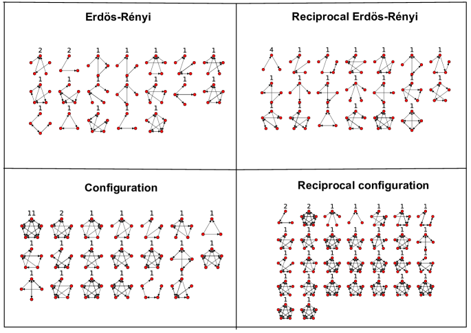
Supplementary Fig. S2: Different motif sets obtained with the four base models. Inferred motif sets of the best model for the right hemisphere of the Drosophila larva MBs connectome. In this specific application, over all inferences across base models, the configuration model captures the lowest codelength. We observe a particularly clear distinction in the main types of motifs between Erdős-Rényi-like and configuration like models.

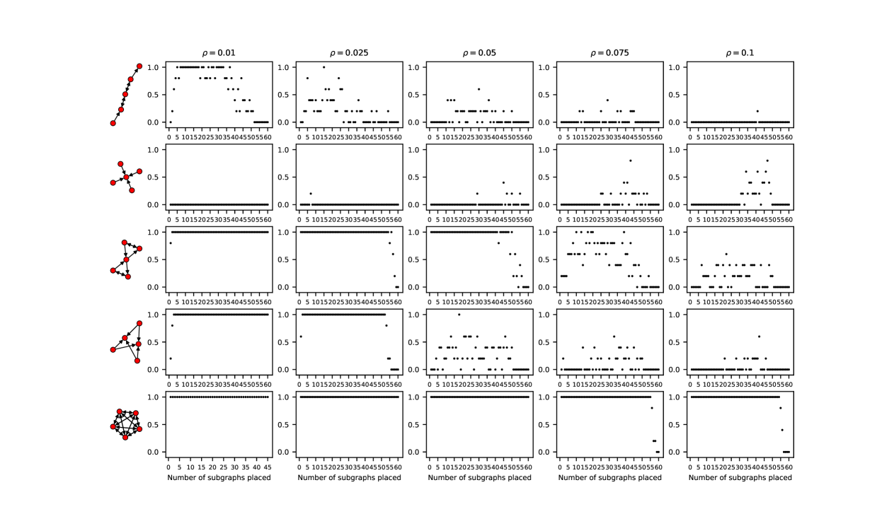
Supplementary Fig. S3: Probability of correctly identifying the motif in the planted motif model. Probability of the inferred motif set containing at least one repetition of the true planted motif as a function of the number of times the motif is planted for five different planted motifs and for different network densities. The generated networks contain $N=300$ nodes and the edge density ranges from $\rho=0.01$ (leftmost) to $\rho=0.1$ (rightmost). Each point is an average over five independently generated graphs.

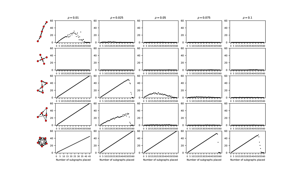
Supplementary Fig. S4: Number of occurrences of the planted motif in the inferred motif set. Denoting by $\alpha$ the planted motif, its number of insertions in the generated graphs, $m_{\alpha}^{*}$ is plotted on the x-axis, and this inferred number, averaged over five independent graphs, is read on the y-axis, $\langle m_{\alpha}^{*}\rangle$. The maximum value of inserted motifs is $\min\left(N/n_{\alpha},E/e_{\alpha}\right)$ ; hence the varying x-axis sizes for $\rho=0.01$. The generated networks contain $N=300$ nodes and the edge density ranges from $\rho=0.01$ (leftmost) to $\rho=0.1$ (rightmost).

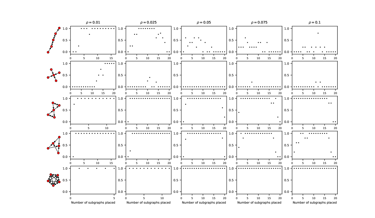
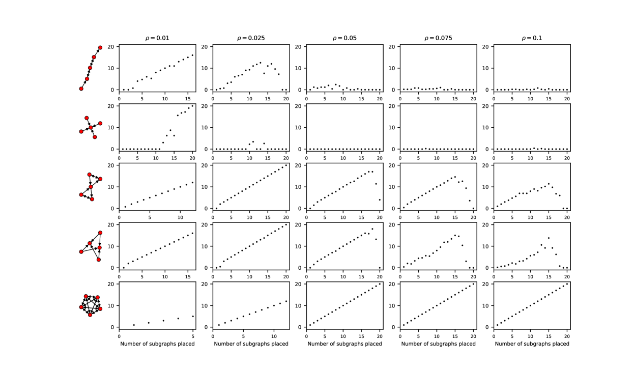
Supplementary Fig. S5: Probability of correctly identifying the motif in the planted motif model. Probability of the inferred motif set containing at least one repetition of the true planted motif as function of the number of times the motif is planted for five different planted motifs and for different network densities. The maximum value of inserted motifs is $\min\left(N/n_{\alpha},E/e_{\alpha}\right)$. The generated networks contain $N=100$ nodes and the edge density ranges from $\rho=0.01$ (leftmost) to $\rho=0.1$ (rightmost).

Supplementary Fig. S6: Number of occurrences of the planted motif in the inferred motif set. Denoting by $\alpha$ the planted motif, its number of insertions in the generated graphs, $m_{\alpha}^{*}$ is plotted on the x-axis, and this inferred number, averaged over five independent graphs, is read on the y-axis, $\langle m_{\alpha}\rangle$. The maximum value of inserted motifs is $\min\left(N/n_{\alpha},E/e_{\alpha}\right)$ ; hence the varying x-axis sizes for $\rho=0.01$. The generated networks contain $N=100$ nodes and the edge density ranges from $\rho=0.01$ (leftmost) to $\rho=0.1$ (rightmost).

Supplementary Fig. S7: Compression of the connectomes obtained with the different base models, with and without motifs. Difference in codelength between the simple Erdős-Rényi (ER) model and each of the other seven models (RER: reciprocal ER model, CM: configuration model, RCM: reciprocal configuration model, ER+Motifs: ER base model with motifs, RER+Motifs: reciprocal ER base with motifs, CM+Motifs: configuration model with motifs, RCM+Motifs: reciprocal configuration model with motifs).

Supplementary Fig. S8: Differences between motifs inferred in an empirical connectome when using different null models. (A) Number of apparent motifs inferred in Drosophila larva right mushroom body connectome when using each of the four null models. Note that even though the reciprocal models are strictly more constrained than their directed counterparts, more motifs are found with these null models than the less constrained ones. (B) Overlap (Jaccard index) between the inferred graphlets using the different null models. (C) Per null model, fraction of uniquely found motifs compared to another null model. Formally, denoting by $\mathcal{M}_{i}$, the motif set wrt. the null model on the $i$-th row, and $\mathcal{M}_{j}$, the motif set wrt. the null model on the $j$-th column, matrix entries are computed as $|\mathcal{M}_{i}\backslash\mathcal{M}_{j}|/|\mathcal{M}_{i}|$. A low ratio indicates that $\mathcal{M}_{j}$ contains most of $\mathcal{M}_{i}$, while a hight ratio expresses strong dissimilarities between the two emerged motif sets.

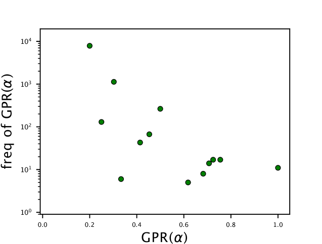
Supplementary Fig. S9: Distribution of graph polynomial root (GPR) values of all 5-node graphlets. The minimum value of the GPR, for five-node graphlets, is 1/5. It would be 0 in an infinite maximally asymmetric graph, e.g., one where the automorphism group is a singleton. A GPR of 1, i.e., its maximum value for any graph size, represent maximally symmetric graphs, e.g., cliques. Symmetry of motif sets in Fig. 5 must be read knowing that the GPR is bounded between 0.2 and 1.

Supplementary Note S1 Subgraph census

Writing graphlet occurrences.

Subgraph-census is a computationally hard task since it involves repeatedly solving the subgraph isomorphism problem. Since our algorithm uses not only the number of occurrences of each graphlet but also their placement in the original graph, we need to not only determine the subgraph isomorphism class sizes but list all weakly connected subgraphs from three to five nodes. There are about 10 000 distinct five-node graphlets, a distribution that can be easily stored on any modern laptop. However, the exhaustive lists of all graphlet occurrences can be drastically large, depending on the size and density of the network at hand. In the case of the brain regions of the adult Drosophila melanogaster, the magnitude of such connectomes is of the order of a thousand neurons, which, for their specific density, leads to at least several billions five-node subgraphs. In this case it is not possible to dynamically store all subgraph occurrences. Instead, we progressively write them to disk directly using textfile pointers thanks to the ifstream object of the C++ standard library (https://cplusplus.com/reference/fstream/ifstream/). Each text file corresponds to a graphlet, containing isomorphic subgraphs divided on each line, with grouped node labels stored in CSV format.

Reading graphlet occurrences.

Uniformly sampling subgraphs is part of our greedy algorithm. Randomizing the collected subgraph lists followed by sequential reading of their elements would be the most direct and simple approach to do this. Since it is not possible to store every induced subgraph in memory, we store the pointer positions of every line (i.e., every subgraph memory address) in a vector. These vector elements are thus shuffled, then read sequentially to perform a uniform sampling of the subgraphs. The memory gain, per graphlet textfile, is of the order of the textfile size times the graphlet size. In large connectomes, this memory gain is however not enough and it is not possible to store all subgraph pointers in memory. For this case, we implemented a procedure that divides the reading and shuffling of a graphlet textfile in chunks of a fixed size. If the number of subgraphs in a graphlet textfile (i.e., its number of lines) is lower than the chunk size, then the sampling is performed as described above. When the graphlet textfile is larger than the chunk size, the subgraph sampling is not uniform. Indeed, the initial node labeling of the input graph, together with the order of the subgraph mining imposed by Wernicke’s algorithm, requires having access to all the listed subgraphs for a sampling to be exactly uniform. The larger the chunk reading size is, the less biased the sampling will be. For all the adult Drosophila melanogaster connectomes, we fixed the chunk size to a million subgraphs, so that the maximum number of stored subgraph pointers in RAM per graphlet is a million. When all the subgraphs of the current chunk of the full graphlet textfile are forbidden by the non-overlapping supernode constraint (cf. Algorithm 2), another chunk is read.

Supplementary Note S2 Subgraph contraction costs

We give in this note closed-form expressions for the putative difference in codelength which would be obtained by contracting a given subgraph in the reduced graph $H_{t}=(\mathcal{N}_{t},\mathcal{E}_{t})$. These are the expressions we use in practice in our greedy algorithm to select the most compressing subgraph at each iteration. The codelength difference for a subgraph contraction depends on the base model used to encode $H_{t}$, so we give below expressions for each of the four base models. We will for notational convenience drop the subscripts pertaining to the iteration $t$ and thus simply refer to $H=(\mathcal{N},\mathcal{E})$ in the remainder of this section.

Common quantities

In all steps, all base models share a cost difference related to the transformation of a group of a entries in the adjacency matrix $\mathbf{A}=\mathbf{A}(H)$ from $[A_{ij}]$ to $[A_{ij}^{\prime}]$ caused by the contraction of a given subgraph $s=({\nu},{\epsilon})\in H$. This difference is given by

$$\ell_{\mathbf{A}}(s) \ =\sum_{i\in{\nu}}\log\left[\frac{k^{+}_{i}(s)!}{\prod_{j\in{\partial s}}A_{ij}!}\times\frac{k^{-}_{i}(s)!}{\prod_{j\in{\partial s}}A_{ji}!}\right],$$ (38)

where the subgraph’s neighborhood ${\partial s}$ is the set of nodes in $H$ that are connected to a node of $s$, and

$$k^{+}_{i}(s) \ =\sum_{j\in{\partial s}}A_{ij},$$ (39)

$$k^{-}_{i}(s) \ =\sum_{j\in{\partial s}}A_{ji}.$$ (40)

Such that the subgraph in- or out-degree is:

$$k^{\pm}(s)=\sum_{i\in\nu}k_{i}^{\pm}(s)$$ (42)

In the following, we will denote by $n=|\nu|$ the subgraph size and by $e=|\epsilon|$ the number of edges $s$ holds. We furthermore denote by $e_{d}=\frac{1}{2}\sum_{i,j\in\nu}|A_{ij}-A_{ji}|$ the number of directed (asymmetric) edges and by $e_{m}=\frac{1}{2}(e-e_{d})$ the number of mutual edges of $s$. The size of $H$ is written $N$, the number of edges $E$, its number of mutual edges $E_{m}$ and its number of (asymmetric) directed edges $E_{d}$.

Base model complexity cost

In our inference of the planted motif model, the entropy of the base model (i.e., its negative log-likelihood), $S_{\phi}$, is not the only term that is affected when contracting a subgraph. The base model parameters $\phi(H)$ also change, which may change the codelength needed to encode them, and must thus also be taken into account in the putative codelength difference. This constitutes a fundamental difference from classical likelihood maximization which protects against overfitting.

Positive integer

We let $a$ denote a positive integer. It could represent a number of edges or nodes, the maximum degree, etc. As was described in the “Compression, model selection, and hypothesis testing” section, $a$ can be encoded using $L_{\mathbb{N}}(a)=\log[a(a+1)]$ bits. Thus, if the contraction of a subgraph $s$ induces the variation $a\longrightarrow a+\Delta a(s)$, then the associated codelength difference is

$$\Delta L_{\mathbb{N}}(a,s)=L_{\mathbb{N}}(a)-L_{\mathbb{N}}(a+\Delta a(s))=\log\frac{a(a+1)}{[a+\Delta a(s)][a+\Delta a(s)+1]}.$$ (43)

For instance, for the ER model, a subgraph contraction changes the base model’s parameters as $\Delta E(s)=-e$ and $\Delta N(s)=1-n$, leading to a change in codelength of

$$\Delta L_{\mathbb{N}}(E,s)=\log\frac{E(E+1)}{[E-e][E-e+1]}$$ (44)

for describing $E$ and of

$$\Delta L_{\mathbb{N}}(N,s)=\log\frac{N(N+1)}{[N-n+1][N-n+2]}$$ (45)

for describing $N$.

Sequences of positive integers

Let $\textbf{a}=(a_{i})$ be a sequence of $N$ positive integers. For our purpose,05 a represents a sequence of node degrees (i.e., the in,- out-, or mutual degrees of $H$).

The sequence $\mathbf{a}$ is described either by a uniform code or a plug-in code (Eqs.  (17),(18) ) that both depend on the range of values distributed in $\mathbf{a}$. We let the maximum value of the sequence be denoted $Q\equiv\max\mathbf{a}$ ($\Delta$ in the main text), and the mininum value $q\equiv\min\mathbf{a}$ ($\delta$ in the main text). For each distinct value $\mu$ in $\mathbf{a}$, we let $r_{\mu}\equiv\sum_{i=1}^{N}\delta(a_{i},\mu)$ denote its frequency.

Let $a(s)\equiv a_{i_{s}}$ be the new sequence element added to $\mathbf{a}$, after $s$ is contracted into a supernode, which is labeled $i_{s}$. It is given by

$$a(s)=\sum_{i\in\nu}a_{i}-a_{0}(s),$$ (46)

where $a_{0}(s)$ is related to the deleted internal edges of $s$ or the concatenation of subgraph neighborhoods into multiedges. Let us review how supernode degrees are computed in the configuration model and its reciprocal conterpart to show that the above expression holds for the present study.

In the case of the configuration model, the evaluation of the out-degree of a new supernode is

$$k^{+}(s) =\sum_{i\in\nu}\sum_{j\in\partial s}A_{ij}$$ (47)

$$=\sum_{i\in\nu}\left(\sum_{j}A_{ij}-\sum_{j\in s}A_{ij}\right)$$ (48)

$$=\sum_{i\in\nu}k_{i}^{+}-e,$$ (49)

such that one identifies $k_{0}(s)=e$. For the in-degree sequence, the expression holds by the change of notation $+\longrightarrow-$.

For the reciprocal configuration model, three degree sequences are involved. Starting with the directed out-degree,

$$\kappa^{+}(s) =\sum_{j\in\partial s}\max\left(\sum_{i\in\nu}(A_{ij}-A_{ji}),0\right)$$ (50)

$$=\frac{1}{2}\sum_{i\in\nu}\sum_{j\in\partial s}(A_{ij}-A_{ji})+\frac{1}{2}\sum_{j\in\partial s}\left|\sum_{i\in\nu}(A_{ij}-A_{ji})\right|$$ (51)

$$=\sum_{i\in\nu}\kappa^{+}_{i}-\kappa_{0}(s),$$ (52)

with

$$\kappa_{0}(s) =e_{d}+\frac{1}{2}\sum_{j\in\partial s}\left(\sum_{i\in\nu}|A_{ij}-A_{ji}|-\left|\sum_{i\in\nu}(A_{ij}-A_{ji})\right|\right).$$ (53)

The directed in-degree is identical after the change of notation $+\longrightarrow-$. The mutual degree of a supernode is simply given by its relationship to the configuration model’s in- (or out-) degree and to the mutual degree,

$$\kappa^{m}(s) =k^{+}(s)-\kappa^{+}(s)=k^{-}(s)-\kappa^{-}(s)$$ (54)

$$=\sum_{i\in s}(k_{i}^{+}-\kappa_{i}^{+})-[k_{0}(s)-\kappa_{0}(s)]$$ (55)

$$=\sum_{i\in s}\kappa^{m}_{i}-\kappa_{0}^{m}(s)$$ (56)

The supernode degree and node degrees of the subgraph’s nodes are not the only sequence elements modified by the subgraph contraction. Properties of the subgraph’s neighborhood are also likely to evolve if degree sequences are correlated, which is the case of the reciprocal configuration model. After the contraction of $s$, we will denote by $\Delta a_{j}(s)$, the variation of the element $a_{j}\longrightarrow a_{j}+\Delta a_{j}(s)$, associated to a network property of node $j\in\partial s$. Variations of the directed in- and out-degrees are equal:

$$\Delta\kappa^{+}_{j}(s) =\max\left(\sum_{i\in\nu}(A_{ji}-A_{ij}),0\right)-\sum_{i\in\nu}\max(A_{ji}-A_{ij},0)$$

$$=\frac{1}{2}\left|\sum_{i\in\nu}(A_{ji}-A_{ij})\right|-\frac{1}{2}\sum_{i\in\nu}|A_{ji}-A_{ij}|$$

$$=\Delta\kappa_{j}^{-}(s)\equiv\Delta\kappa_{j}(s)$$ (57)

The case of the mutual degree is deduced by the conservation of the in- and out-degree of the subgraph’s neighbors:

$$\Delta k_{j}^{+}(s) =\Delta k_{j}^{-}(s)=0$$ (58)

$$\Leftrightarrow\Delta\kappa_{j}^{m}(s) =-\Delta\kappa_{j}(s)$$ (59)

One can write how the distribution $\{r_{\mu}\}$ transforms into $\{r_{\mu}+\Delta r_{\mu}(s)\}$.

$$\Delta r_{\mu}(s)=\delta(a(s),\mu)-\sum_{i\in s}\delta(a_{i},\mu)+\sum_{j\in\partial s}[\delta(a_{j}+\Delta a_{j}(s),\mu)-\delta(a_{j},\mu)]$$ (60)

Updates of $Q\longrightarrow Q+\Delta Q(s)$ and $q\longrightarrow q+\Delta q(s)$ are naturally determined by the evolution of the sequence $\mathbf{a}\longrightarrow\mathbf{a}+\Delta\mathbf{a}(s)$, and by how the distribution $\{r_{\mu}\}$ of its elements is shifted by the contraction of $s$, $\{\Delta r_{\mu}(s)\}$. Consider first the case of the upate of the maximum. A first scenario could be an augmentation of the maximum, $\Delta Q(s)>0$, by either the new supernode or an increase of a subgraphs’s neighbor degree, i.e., $\Delta a_{j}(s)>0$. Let $Q^{\prime}(s)$ be the maximum between a supernode degree and one of the updated subgraph’s neighbors degrees:

$$Q^{\prime}(s)=\max\left(a(s),\max_{j\in\partial s}\{a_{j}+\Delta a_{j}(s)\}\right)$$ (61)

A second scenario, when $Q^{\prime}(s)<Q$, is the possible extinction of the maximum, i.e., $\Delta r_{Q}(s)=-r_{Q}$. Introducing the quantity $\Delta Q^{\prime}(s)=\max(Q^{\prime}(s)-Q,0)$, the difference in maxima is expressed as

$$\Delta Q(s) =\Delta Q^{\prime}(s)+\delta(\Delta Q^{\prime}(s),0)\delta(\Delta r_{Q}(s),-r_{Q})\sum_{\mu=0}^{Q-1}(\mu-Q)\mathfrak{g}_{\mu}^{Q}(s)$$ (62)

where $\mathfrak{g}_{\mu}^{Q}(s)$ in an indicator function that returns 1 when $\mu$ is the highest value below $Q$ in $\mathbf{a}$ after the update, and 0 otherwise. It can be formally written as:

$$\mathfrak{g}_{\mu}^{Q}(s)=\left[1-\delta(\Delta r_{\mu}(s),-r_{\mu})\right]\prod_{\mu^{\prime}=\mu+1}^{Q-1}\delta(\Delta r_{\mu^{\prime}}(s),-r_{\mu^{\prime}})$$ (63)

The first term on the RHS of Eq.62 corresponds to the case where the maximum of the sequence is increased by the insertion of a supernode or the restructuring of the subgraph’s neighborhood. The second term is the alternative scenario where the maximum is decreased and must be searched within $\mathbf{a}$.

The variation in minima $\Delta q(s)$ is naturally similar to Eq.62. Let $q^{\prime}(s)$ be the minimum between a supernode degree and one the updated subgraph’s neighbor degrees:

$$q^{\prime}(s)=\min\left(a(s),\min_{j\in\partial s}\{a_{j}+\Delta a_{j}(s)\}\right)$$ (64)

Introducing $\Delta q^{\prime}(s)=-\min(q-q^{\prime}(s),0)$, the difference in minima is expressed as

$$\Delta q(s)=\Delta q^{\prime}(s)+\delta(\Delta q^{\prime}(s),0)\delta(\Delta r_{q}(s),-r_{q})\sum_{\mu=q+1}^{Q+\Delta Q(s)}(\mu-q)\mathfrak{g}_{\mu}^{q}(s)$$ (65)

where $\mathfrak{g}_{\mu}^{q}(s)$ in an indicator function that returns 1 when $\mu$ is the lowest value greater than $q$ in $\mathbf{a}$ after the update, and 0 otherwise. It can be formally written as:

$$\mathfrak{g}_{\mu}^{q}(s)=\left[1-\delta(\Delta r_{\mu}(s),-r_{\mu})\right]\prod_{\mu^{\prime}=q+2}^{\mu}\delta(\Delta r_{\mu^{\prime}}(s),-r_{\mu^{\prime}})$$ (66)

The first term on the RHS of Eq.65 corresponds to the case where the minimum of the sequence is decreased by the insertion of a supernode or the restructuring of the subgraph’s neighborhood. The second term is the alternative scenario where the minimum is increased and must be searched within $\mathbf{a}$.

All necessary quantities involved in putative codelength differences of integer sequences have been determined. Let us now give their exact expressions.

Uniform code

A uniform encoding of $\mathbf{a}$ corresponds to $N$ products of a uniform probability distribution over $q$ to $Q$,

$$L_{U}(\mathbf{a})=N\log(Q-q+1)+L_{\mathbb{N}}(Q)+L_{\mathbb{N}}(q).$$ (67)

The codelength difference is

$$\Delta L_{U}(\mathbf{a},s) =-N\log\left(1+\frac{\Delta Q(s)-\Delta q(s)}{Q-q+1}\right)+(n-1)\log(Q-q+1)$$ (68)

$$+\Delta L_{\mathbb{N}}(Q,s)+\Delta L_{\mathbb{N}}(q,s).$$

Plug-in code

The plug-in code is a function of $\{r_{\mu}\}$ and a hyperparameter $\lambda$, that constrains the shape of the prior. Two different values for $\lambda$ were considered in the main text, $\lambda=1/2$ (Jeffreys prior) and $\lambda=1$ (uniform prior). The plug-in code of a sequence is characterized by three entities: $N$, $\{r_{\mu}\}_{q\leq\mu\leq Q}$, and $\Lambda\equiv\Lambda(Q,q)=(Q-q+1)\lambda$:

$$L_{\lambda}(\mathbf{a})=\log\frac{\Gamma(N+\Lambda)}{\Gamma(\Lambda)}+(Q-q+1)\log\Gamma(\lambda)-\sum_{q\leq\mu\leq Q}\log\Gamma(r_{\mu}+\lambda).$$ (69)

Let $\Delta\Lambda(Q,q,s)$ the variation following the contraction of $s$, $\Lambda(Q,q)\longrightarrow\Lambda(Q,q)+\Delta\Lambda(Q,q,s)$. The latter is determined by how the maximum and minimum of $Q$ and $q$ are closer or more distant after the subgraph contraction. One can independently treat the case where $Q$ or $q$ changes. Thus, we adopt the following decomposition,

$$\Delta\Lambda(Q,q,s) =\Delta\Lambda(Q,s)+\Delta\Lambda(q,s)$$ (70)

$$=[\Delta Q(s)-\Delta q(s)]\lambda$$ (71)

The update of the plug-in code after a subgraph contraction is divided into multiple cases, depending on how the contraction of a subgraph $s$ affects $N$, $\{r_{\mu}\}_{q\leq\mu\leq Q}$, and $\Lambda(Q,q)$. All in all, the plug-in codelength difference is

$$\Delta L_{\lambda}(\mathbf{a},s) =\log\frac{\Gamma(N+\Lambda)}{\Gamma(N-n+1+\Lambda+\Delta\Lambda(Q,q,s))}+\log\frac{\Gamma(\Lambda+\Delta\Lambda(Q,q,s))}{\Gamma(\Lambda)}$$ (72)

$$+\sum_{\mu=\mu_{\textrm{min}}}^{\mu_{\textrm{max}}}\log\frac{\Gamma(r_{\mu}+\Delta r_{\mu}(s)+\lambda)}{\Gamma(r_{\mu}+\lambda)}+\Delta L_{\mathbb{N}}(N,s)+\Delta L_{\mathbb{N}}(Q,s)+\Delta L_{\mathbb{N}}(q,s),$$

where $\mu_{\textrm{min}}=\min(q,q+\Delta q(s))$ and $\mu_{\textrm{max}}=\max(Q,Q+\Delta Q(s))$.

Erdős-Rényi model

For the ER model, $(N,E)$ will change to $(N-n+1,E-e)$ after the contraction of $s$. The putative codelength difference is then given by

$$\Delta L_{{(N,E)}}(H,s) =e\log[(N-n)(N-n+1)]+E\log\frac{N(N-1)}{(N-n)(N-n+1)}$$ (73)

$$\quad-\log\frac{E!}{(E-e)!}-\ell_{\mathbf{A}}(s).$$

Reciprocal Erdős-Rényi model

For the reciprocal ER model, the variation of the number of mutual edges and directed edges do not only depend on $e_{d}$ and $e_{m}$ because the formation of multiedges (as stacked single edges) changes the number of mutual edges $E_{m}$ and the number directed edges $E_{d}$ in $H$. First, let us write those variations. The variation of the number of mutual edges $\Delta E_{m}(s)$ and of the number of directed edges $\Delta E_{d}(s)$ are given by

$$\Delta E_{m}(s) =-e_{m}+\sum_{j\in\partial s}\left[\min\left(\sum_{i\in\nu}A_{ij},\sum_{i\in\nu}A_{ji}\right)-\sum_{i\in\nu}\min(A_{ij},A_{ji})\right]$$ (74)

$$=-e_{m}+\frac{1}{2}\sum_{j\in\partial s}\left(\sum_{i\in\nu}|A_{ij}-A_{ji}|-\left|\sum_{i\in\nu}(A_{ij}-A_{ji})\right|\right),$$ (75)

and

$$\Delta E_{d}(s)= -e-2\Delta E_{m}(s)$$ (76)

$$= -e_{d}-\sum_{j\in\partial s}\left(\sum_{i\in\nu}|A_{ij}-A_{ji}|-\left|\sum_{i\in\nu}(A_{ij}-A_{ji})\right|\right).$$ (77)

The codelength has two part, one for the directed edges and another for the mutual edges. For the directed edges, one can adapt Eq.73, and replace $e$ by $\Delta E_{d}(s)$:

$$\Delta L_{(N,E_{d})}(H^{\mathrm{asym}},s) =-\Delta E_{d}(s)\log\left[(N-n)(N-n+1)\right]+E_{d}\log\frac{N(N-1)}{(N-n)(N-n+1)}$$

$$\quad-\log\frac{E_{d}!}{(E_{d}+\Delta E_{d}(s))!}-\ell_{\mathbf{A}^{\mathrm{asym}}}(s).$$ (78)

For the mutual part, the putative codelength difference is:

$$\Delta L_{(N,E_{m})}(H^{\mathrm{sym}},s) =-\Delta E_{m}(s)\log\left[\frac{(N-n)(N-n+1)}{2}\right]+E_{m}\log\frac{N(N-1)}{(N-n)(N-n+1)}$$

$$\quad-\log\frac{E_{m}!}{(E_{m}+\Delta E_{m}(s))!}-\ell_{\mathbf{A}^{\mathrm{sym}}}(s).$$ (79)

where $\ell_{\mathbf{A}^{\mathrm{sym}}}(s)$ is the undirected version of Eq.38, where only one of two terms inside the $\log$ needs to be kept.

Finally, the codelength difference can be written as

$$\Delta L_{{(N,E_{m},E_{d})}}(H,s)=\Delta L_{(N,E_{d})}(H^{\mathrm{asym}},s)+\Delta L_{(N,E_{m})}(H^{\mathrm{sym}},s)$$ (80)

Configuration model

The codelength difference when contracting a subgraph $s$ for the configuration model is

$$\Delta L_{H,{(\mathbf{k}^{+},\mathbf{k}^{-})}}(s) =\log\frac{E!}{(E-e)!}+\log\left[\frac{k^{+}(s)!}{\prod_{i\in{\nu}}k^{+}_{i}!}\times\frac{k^{-}(s)!}{\prod_{i\in{\nu}}k^{-}_{i}!}\right]-\ell_{\mathbf{A}}(s),$$ (81)

where $k^{+}_{i}=k^{+}_{i}(H)$, and $k^{-}_{i}=k^{-}_{i}(H)$ as above, and

$$k^{\pm}(s) \ =\sum_{i\in{\nu}}k^{\pm}_{i}(s)=\sum_{i\in{\nu}}k^{\pm}_{i}-e.$$ (82)

Reciprocal configuration model

Finally, the codelength difference for the reciprocal configuration model is equal to

$$\Delta L_{{(\bm{\kappa}^{m},\bm{\kappa}^{+},\bm{\kappa}^{-})}}(H,s) =\log\frac{E_{d}!}{[E_{d}+\Delta E_{d}]!}+\log\frac{(2E_{m}-1)!!}{[2(E_{m}+\Delta E_{m})-1]!!}$$

$$\quad+\log\left[\frac{\kappa^{+}(s)!}{\prod_{i\in{\nu}}\kappa_{i}^{+}!}\times\frac{\kappa^{-}(s)!}{\prod_{i\in{\nu}}\kappa_{i}^{-}!}\times\ \frac{\kappa^{m}(s)!}{\prod_{i\in{\nu}}\kappa^{m}_{i}!}\right]$$

$$\quad+\sum_{j\in\partial s}\log\left[\frac{(\kappa^{+}_{j}+\Delta\kappa_{j}(s))!}{\kappa_{j}^{+}!}\times\frac{(\kappa^{-}_{j}+\Delta\kappa_{j}(s))!}{\kappa_{j}^{-}!}\times\ \frac{(\kappa^{m}_{j}-\Delta\kappa_{j}(s))!}{\kappa^{m}_{j}!}\right]$$

$$\quad-\ell_{\mathbf{A}^{\text{asym}}}(s)-\ell_{\mathbf{A}^{\text{sym}}}(s).$$ (83)

where

$$\kappa^{\pm}(s) =\sum_{i\in\nu}\kappa_{i}^{\pm}(s)=\sum_{i\in\nu}\kappa^{\pm}_{i}+\frac{1}{2}\Delta E_{d}(s)-\frac{e_{d}}{2}$$ (84)

$$\kappa^{m}(s) =\sum_{i\in\nu}\kappa_{i}^{m}(s)=\sum_{i\in\nu}\kappa_{i}^{m}+\Delta E_{m}(s)$$ (85)

are respectively the directed and mutual degrees of the future supernode. The $\{\Delta\kappa_{j}(s)\}_{j\in\partial s}$ are respectively variations of the directed degrees of the subgraph neighborhood due to its contraction (cf. Eq.57 for their expressions).

Supplementary Note S2.1 Planted motif model

Based on the previous subsections, we can give the complete putative codelength difference when contracting a subgraph. As a reminder, the codelength of our model is

$$L(G,\theta)=L(\Gamma,\mathcal{S})+L(H,\phi)+L(\mathcal{V}|H,\mathcal{S})+L(G|H,\mathcal{V},\mathcal{S},\Gamma),$$ (86)

where $\theta=\{H,\phi,\mathcal{S},\mathcal{V},\Gamma\}$. $H$ is the reduced colored multigraph, $\Gamma$ is the set of all discovered graphlets, $\mathcal{S}$ is the graphlet multiset (a proxy for a set of subgraphs), $\mathcal{V}$ are $H$’s node labels identifying supernodes, and $\phi$ are the parameters of the dyadic base model. Let us give the subgraph-contraction-induced cost for all terms of the above equation.

The update of the encoding cost of the graphlet set and multiset, $L(\Gamma,\mathcal{S})$ (cf. Eq.(6)), is seen as an extension of $\mathcal{S}$ by $\alpha$, the label of the graphlet to which $s$ is isomorphic. We choose to encode $\mathcal{S}$ as an ordered multiset of elements, that are independently sampled from $\Gamma$ and their respective frequency in $\mathcal{S}$ is encoded by a uniform distribution over the range one to $m_{\textrm{max}}$. The minimum value of $m_{\textrm{max}}$ is one. Two exclusive scenarios may occur for a non-zero update cost. Either an occurrence of the most represented graphlet in $\mathcal{S}$ is again selected and leads to an incremental increase of $m_{\textrm{max}}$, or $s$ is isomorphic to a different $\alpha\notin\mathcal{S}$. Denoting by $\mathcal{A}$ the unique set of elements of $\mathcal{S}$,

$$\Delta L(\Gamma,\mathcal{S},s)=-\delta(m_{\alpha},m_{\text{max}})\left[|\mathcal{A}|\log\left(1+\frac{1}{m_{\textrm{max}}}\right)+\log\left(1+\frac{2}{m_{\textrm{max}}}\right)\right]-\delta(m_{\alpha},0)\left(\log|\Gamma|+\log m_{\text{max}}\right)$$ (87)

The update of the encoding of the supernode labels, $L(\mathcal{V}|H,\mathcal{S})$ (cf. Eq.7), is, again, affected by the graph size, the growth of the supernode number and the incremental increase of a graphlet occurrence. Denoting by $M\equiv\sum_{\alpha^{\prime}}m_{\alpha^{\prime}}=|\mathcal{S}|$ the number of supernodes,

$$\Delta L(\mathcal{V},s|H,\mathcal{S})=\log\left(\frac{m_{\alpha}+1}{M+1}\right)+\log\binom{N}{M}-\log\binom{N-n+1}{M+1}$$ (88)

The update of reconstruction cost from $H$ to $G$ depends on the reduced graph size, the associated graphlet orientation number and the subgraph’s neighborhood:

$$\Delta L(G,s|H,\mathcal{V},\mathcal{S},\Gamma) =\log\frac{(N-n+1)!}{N!}+\frac{n_{\alpha}!}{|\mathrm{Aut}(\alpha)|}$$ (89)

$$+\sum_{j\in\mathcal{N}(H)\backslash\mathcal{V}}\log\binom{n}{\sum_{i\in\nu}A_{ij}}\binom{n}{\sum_{i\in\nu s}A_{ji}}+\sum_{j_{s^{\prime}}\in\mathcal{V}}\log\binom{nn_{j_{s}^{\prime}}}{\sum_{i\in\nu}A_{ij_{s^{\prime}}}}\binom{nn_{j_{s}^{\prime}}}{\sum_{i\in\nu}A_{j_{s^{\prime}}i}},$$

where $n_{j_{s}^{\prime}}$ is the subgraph size relative to the supernode $j_{s^{\prime}}\in\mathcal{V}$, replacing the subgraph $s^{\prime}$. The two sums represent the encoding of the nodes’ neighbours within $s$, i.e., how to distribute the multiedge among the nodes that would be deleted. The first sum correponds to regular node neighbors, while the second sum corresponds to supernode neighbors.

Finally, the complete putative codelength difference is:

$$\Delta L(G,\theta,s)=\Delta L_{\phi}(H,s)+\Delta L(\phi,s)+\Delta L(G,s|H,\mathcal{V},\mathcal{S},\Gamma)+\Delta L(\mathcal{V},s|H,\mathcal{S})+\Delta L(\Gamma,\mathcal{S},s)$$ (90)

Supplementary Note S3 Entropy of simple the reciprocal configuration model

To derive the entropy of the reciprocal configuration model for simple graphs, we follow the approach developed in [69]. Compared to the directed configuration model, the reciprocal version has the mutual degree sequence, i.e., the number of mutual stubs (corresponding to reciprocal edges) per node, as an additional set of parameters. We let $\mathbf{u}$ denote a vector of size $N$ filled with ones, and we define the microcanonical partition function as a sum over a product of Dirac delta functions which define the constrained parameter values of the model,

$$\Omega{(\bm{\kappa}^{m},\bm{\kappa}^{+},\bm{\kappa}^{-})}=\sum_{\mathbf{A}}\delta\left(\bm{\kappa}^{m}-v_{D}\left(\mathbf{AA}^{T}\right)\right)\delta\left(\bm{\kappa}^{+}-\mathbf{Au}+v_{D}\left(\mathbf{AA}^{T}\right)\right)\delta\left(\bm{\kappa}^{-}-\mathbf{A}^{T}\mathbf{u}+v_{D}\left(\mathbf{AA}^{T}\right)\right),$$ (91)

where $v_{D}$ is a function that maps the diagonal elements of a $N\times N$ matrix to a $N$-dimensional vector. The Dirac delta functions can be expanded in terms of Fourier integrals to obtain:

$$\Omega{(\bm{\kappa}^{m},\bm{\kappa}^{+},\bm{\kappa}^{-})} =\int\frac{\text{d}\bm{\lambda}^{+}\text{d}\bm{\lambda}^{-}\text{d}\bm{\mu}}{(2\pi)^{3N}}\ e^{{\bm{\lambda}^{+}}^{T}\bm{\kappa}^{+}+{\bm{\lambda}^{-}}^{T}\bm{\kappa}^{-}+\bm{\mu}^{T}\bm{\kappa}^{m}}\sum_{\mathbf{A}}e^{-{\bm{\lambda}^{+}}^{T}\mathbf{Au}-{\bm{\lambda}^{-}}^{T}\mathbf{A}^{T}\mathbf{u}-{\bm{\mu}}^{T}\mathrm{diag}\left(\mathbf{AA}^{T}\right)},$$ (92)

where $\bm{\lambda}^{+},\bm{\lambda}^{-},\bm{\mu}$ are identified as vectors of Lagrange multipliers.

Compared to the classical configuration model, symmetric pairs of elements of the adjacency matrix are not independent and need to be considered simultaneously, such that

$$\sum_{\mathbf{A}}e^{-{\bm{\lambda}^{+}}^{T}\mathbf{Au}-{\bm{\lambda}^{-}}^{T}\mathbf{A}^{T}\mathbf{u}-{\bm{\mu}}^{T}\mathrm{diag}\left(\mathbf{AA}^{T}\right)} =\sum_{\{A_{ij},A_{ji}\}=\{\{0,0\},\{1,1\},\{0,1\},\{1,0\}\}}e^{-\sum_{ij}(\mu_{i}-\lambda_{i}^{+}-\lambda_{i}^{-})A_{ij}A_{ji}}e^{-\sum_{ij}(\lambda_{i}^{+}+\lambda_{j}^{-})A_{ij}}$$

$$=\prod_{i<j}\left(1+e^{-\mu_{i}-\mu_{j}}+e^{-\lambda_{i}^{+}-\lambda_{j}^{-}}+e^{-\lambda_{i}^{-}-\lambda_{j}^{+}}\right).$$ (93)

For the sake of readability, we set $s_{ij}\equiv e^{-\mu_{i}-\mu_{j}}+e^{-\lambda_{i}^{+}-\lambda_{j}^{-}}+e^{-\lambda_{j}^{+}-\lambda_{i}^{-}}$. To estimate $\Omega{(\bm{\kappa}^{m},\bm{\kappa}^{+},\bm{\kappa}^{-})}$, we apply a Laplace approximation to its Fourier integral form, and we thus we seek the maximisation of the following quantity

$$NQ(\bm{\mu},\bm{\lambda}^{+},\bm{\lambda}^{-}|\bm{\kappa}^{m},\bm{\kappa}^{+},\bm{\kappa}^{-})={\bm{\mu}}^{T}\bm{\kappa}^{m}+{\bm{\lambda}^{+}}^{T}\bm{\kappa}^{+}+{\bm{\lambda}^{-}}^{T}\bm{\kappa}^{-}+\sum_{i<j}\ln(1+s_{ij}).$$ (94)

The saddle point equations to be solved are thus

$$\frac{\partial Q}{\partial\mu_{i}}=0 \Leftrightarrow\kappa^{m}_{i}=e^{-\mu_{i}}\sum_{j\neq i}\frac{e^{-\mu_{j}}}{1+s_{ij}},$$ (95)

$$\frac{\partial Q}{\partial\lambda_{i}^{+}}=0 \Leftrightarrow\kappa^{+}_{i}=e^{-\lambda_{i}^{+}}\sum_{j\neq i}\frac{e^{-\lambda_{j}^{-}}}{1+s_{ij}},$$ (96)

$$\frac{\partial Q}{\partial\lambda_{i}^{-}}=0 \Leftrightarrow\kappa^{-}_{i}=e^{-\lambda_{i}^{-}}\sum_{j\neq i}\frac{e^{-\lambda_{j}^{+}}}{1+s_{ij}}.$$ (97)

Here, we are only interested in the sparse graph approximation. The computation of the Hessian would be compulsory in a rigorous calculation. However, when actually evaluated, it only leads to sums of log terms in the degree sequences elements, which are negligible compared to the sums of log factorial terms in the degree sequence elements (when the graph is of finite size). This is the same observation that is found in [69], while never explicitly justified there. For our results to be consistent with the standard form of other simple network entropy expressions, we also choose to neglect the contribution of the Hessian to the sparse graph approximation of the microcanonical partition function.

At large $N$, it is reasonable to assume $s_{ij}=o(1)$ for the right hand terms of the saddle point equations to be finite. This leads to the simplified equations

$$\kappa^{m}_{i} =K_{m}e^{-\mu_{i}}, K_{m}=\sum_{j}e^{-\mu_{j}}$$ (98)

$$\kappa^{+}_{i} =K_{-}e^{-\lambda^{+}_{i}}, K_{-}=\sum_{j}e^{-\lambda_{j}^{-}}$$ (99)

$$\kappa^{-}_{i} =K_{+}e^{-\lambda^{-}_{i}}, K_{+}=\sum_{j}e^{-\lambda_{j}^{+}}$$ (100)

The constants $K_{m},K_{+},K_{-}$ are determined by global structural constraints, which are the number of asymmetrically connected (or directed) pairs of nodes and the number of mutual edges:

$$2E_{m} =\sum_{i}\kappa^{m}_{i}=K_{m}^{2}\Leftrightarrow K_{m}=\sqrt{2E_{m}},$$ (101)

$$E_{d} =\sum_{i}\kappa^{+}_{i}=K_{+}K_{-}\Leftrightarrow K_{+}=K_{-}=\sqrt{E_{d}}.$$ (102)

All is now set for a second-order estimation of the microcanonical partition function in $s_{ij}$. We have

$$\bm{\mu}^{T}\bm{\kappa}^{m} =-\sum_{i}\kappa^{m}_{i}\ln\kappa^{m}_{i}+E_{m}\ln(2E_{m})\approx\ln\frac{(2E_{m})!!}{\prod_{i}\kappa^{m}_{i}!}-E_{m},$$ (103)

$${\bm{\lambda}^{+}}^{T}\bm{\kappa}^{+}+{\bm{\lambda}^{-}}^{T}\bm{\kappa}^{-} =-\sum_{i}\kappa^{+}_{i}\ln\kappa^{+}_{i}-\sum_{i}\kappa^{-}_{i}\ln\kappa^{-}_{i}+E_{d}\ln E_{d}\approx\ln\frac{E_{d}!}{\prod_{i}\kappa^{+}_{i}!\kappa^{-}_{i}!}-E_{d},,$$ (104)

$$s_{ij} =\frac{\kappa^{m}_{i}\kappa^{m}_{j}}{2E_{m}}+\frac{\kappa^{+}_{i}\kappa^{-}_{j}+\kappa^{-}_{i}\kappa^{+}_{j}}{E_{d}},$$ (105)

and

$$\frac{1}{2}\sum_{ij}\left(s_{ij}-\frac{s_{ij}^{2}}{2}\right) =E_{m}+E_{d}-\frac{1}{2}\underbrace{\left(\frac{1}{2}\frac{\langle{\kappa^{m}_{i}}^{2}\rangle^{2}}{\langle\kappa^{m}_{i}\rangle^{2}}+\frac{\langle{\kappa^{+}_{i}}^{2}\rangle\langle{\kappa^{-}_{i}}^{2}\rangle}{\langle\kappa^{+}_{i}\rangle\langle\kappa^{-}_{i}\rangle}+\frac{\langle\kappa^{+}_{i}\kappa^{-}_{i}\rangle^{2}}{\langle\kappa^{+}_{i}\rangle\langle\kappa^{-}_{i}\rangle}+\frac{\langle\kappa^{m}_{i}\kappa^{+}_{i}\rangle\langle\kappa^{m}_{i}\kappa^{-}_{i}\rangle}{\langle\kappa^{m}_{i}\rangle\langle\kappa^{+}_{i}\rangle}\right)}_{\Psi{(\bm{\kappa}^{m},\bm{\kappa}^{+},\bm{\kappa}^{-})}}.$$ (106)

Putting it all together we obtain

$$L_{(\bm{\kappa}^{m},\bm{\kappa}^{+},\bm{\kappa}^{-})}(G)=\log\frac{(2E_{m})!!}{\prod_{i}\kappa^{m}_{i}!}+\log\frac{E_{d}!}{\prod_{i}\kappa^{+}_{i}!\kappa^{-}_{i}!}-\frac{1}{2\ln 2}\Psi{(\bm{\kappa}^{m},\bm{\kappa}^{+},\bm{\kappa}^{-})}.$$ (107)

Similarly to the sparse approximation of entropy of the simple graph configuration model [69], we see that the entropy for the simple graph reciprocal configuration model amounts to the multigraph codelength from which is subtracted a functional cut-off that depends on the statistics of the degree sequences.

Supplementary Note S4 Motif mining based on hypothesis testing

Given a graphlet $\alpha$, hypothesis-based motif inference qualifies $\alpha$ as a network motif in an empirical network $G$ if its frequency $f_{\alpha}(G)$ in $G$ is significantly greater than in an ensemble of random networks $\mathcal{G}_{\theta}$ sampled from a null model $P_{\theta}$.

For uniformly sampling simple random networks, we use the shuffling algorithms described in Randomized networks in the Methods section. When the edge swapping procedures are ergodic and unbiased, they are guaranteed to uniformly sample the corresponding ensembles of random networks after a large enough number of swaps [28]. However, the mixing time, i.e., the number of swaps needed for the generated networks to be practically independent, is not known in general [28]. To ensure that correlations between randomized networks are not likely to influence results (and thus favor hypothesis-testing based methods as much as possible), we perform $100E$ successful edge swaps to generate each random network. This does not guarantee an absence of correlations, but we note that the number of swaps is larger than what is typically prescribed in the literature (for reference 0.2E edge-swaps were used to generate each random network in [16], 3E in [101] and 6E in [60]).

We utilize the typical normality assumption of the graphlet frequencies under the null and employ as test statistic the $Z$-score given by

$$Z_{\alpha,\theta}(G) =\frac{f_{\alpha}(G)-\mu_{\alpha,\theta}}{{\sigma}_{\alpha,\theta}},$$ (108)

where

$$\mu_{\alpha,\theta} =\frac{1}{|\mathcal{G}_{\theta}|}\sum_{G^{\prime}\in\mathcal{G}_{\theta}}f_{\alpha}(G^{\prime})$$ (109)

and

$${\sigma}^{2}_{\alpha,\theta} =\frac{1}{|\mathcal{G}_{\theta}|-1}\sum_{G^{\prime}\in\mathcal{G}_{\theta}}\left[f_{\alpha}^{2}(G^{\prime})-{\mu}^{2}_{\alpha,\theta}\right].$$ (110)

In all experiments, the size of $\mathcal{G}_{\theta}$ is set to 100 and the significance threshold (nominal alpha-level) is fixed at 0.01. To correct for multiple testing (one test for each graphlet), we employ a Bonferroni correction, which multiplies the raw $p$-values obtained directly from the $Z$-scores by $|\Gamma|\approx 10^{4}$. As displayed in Fig. 3A–D, depending on the choice of the null, a considerable number of motifs can be falsely detected. A similar effect can also be seen in empirical data, where the number of motifs found varies enormously with the choice of null model (Supplementary Fig. S8), even though we corrected for multiple testing with the maximally conservative Bonferroni correction. Supplementary Fig. S8 also demonstrates that the motifs found vary significantly depending on the null, and that the smallest number of motifs is not necessarily found under the most restricted null hypothesis.

Supplementary Note S5 Measures of graphlet topology

The density $\rho$ measures the ratio fraction of node pairs in a simple graph $G=(N,E)$ that are connected by an edge [81],

$$\rho=\frac{E}{N(N-1)}.$$ (111)

A simple graph is said to be sparse if its density is close to zero, and dense if its density is close to one.

The reciprocity $r$ measures the fraction of edges in a graph $G$ that are reciprocated [81],

$$r=\frac{1}{E}\sum_{ij}A_{ij}A_{ji},$$ (112)

where $A_{ij}\in\{0,1\}$ are the entries of the adjacency matrix for $G$.

The number of cycles of a simple graph $G$ is the number of closed paths in $G$ where no node appears twice [81].

The graph polynomial root GPR is a measure of the symmetry of a graph. It is related to the so-called orbit-polynomial [80] $\Pi_{G}(z)$ and allows a ranking of graphs based on the distribution of their orbit sizes. Let $c_{o_{l}}$ be the number of orbits of size $o_{l}$, where $l\in\{1,2,\ldots,L\}$ and $L$ is the number of different orbit sizes. The graph polynomial is then defined as

$$\Pi_{G}(z)=\sum_{l=1}^{L}c_{o_{l}}z^{o_{l}}.$$ (113)

The GPR, denoted $z^{*}$, is the unique solution of the following equation

$$\Pi_{G}(z^{*})=1,$$ (114)

which can be solved numerically. Orbit sizes are determined using McKay’s nauty algorithm [102]. A strong degree of symmetry is affiliated with a high GPR, while an asymmetric structure corresponds to a low GPR. Supplementary Figure S9 shows the values of the GPR of all 9 364 three- to five-node graphlets.

References

- 1. Newman ME. The structure and function of complex networks. SIAM review. 2003;45(2):167–256.
- 2. Fornito A, Zalesky A, Bullmore E. Fundamentals of brain network analysis. Academic Press; 2016.
- 3. Alon U. An introduction to systems biology: design principles of biological circuits. CRC press; 2019.
- 4. Watts DJ, Strogatz SH. Collective dynamics of ‘small-world’networks. nature. 1998;393(6684):440–442.
- 5. Newman M. Networks. Oxford university press; 2018.
- 6. Sporns O, Zwi JD. The small world of the cerebral cortex. Neuroinformatics. 2004;2:145–162.
- 7. Bassett DS, Bullmore ET. Small-world brain networks revisited. The Neuroscientist. 2017;23(5):499–516.
- 8. Barabási AL, Albert R. Emergence of scaling in random networks. science. 1999;286(5439):509–512.
- 9. Cohen R, Erez K, Ben-Avraham D, Havlin S. Resilience of the internet to random breakdowns. Physical review letters. 2000;85(21):4626.
- 10. Pastor-Satorras R, Vespignani A. Epidemic spreading in scale-free networks. Physical review letters. 2001;86(14):3200.
- 11. Seyed-Allaei H, Bianconi G, Marsili M. Scale-free networks with an exponent less than two. Physical Review E. 2006;73(4):046113.
- 12. Newman ME. Modularity and community structure in networks. Proceedings of the national academy of sciences. 2006;103(23):8577–8582.
- 13. Ravasz E. Detecting hierarchical modularity in biological networks. Computational Systems Biology. 2009; p. 145–160.
- 14. Cimini G, Squartini T, Saracco F, Garlaschelli D, Gabrielli A, Caldarelli G. The statistical physics of real-world networks. Nature Reviews Physics. 2019;1(1):58–71.
- 15. Battiston F, Cencetti G, Iacopini I, Latora V, Lucas M, Patania A, et al. Networks beyond pairwise interactions: Structure and dynamics. Physics Reports. 2020;874:1–92. doi:10.1016/j.physrep.2020.05.004.
- 16. Milo R, Shen-Orr S, Itzkovitz S, Kashtan N, Chklovskii D, Alon U. Network Motifs: Simple Building Blocks of Complex Networks. Science. 2002;298(5594):824–827. doi:10.1126/science.298.5594.824.
- 17. Sporns O, Kötter R. Motifs in Brain Networks. PLOS Biology. 2004;2(11):e369. doi:10.1371/journal.pbio.0020369.
- 18. Tran NTL, Mohan S, Xu Z, Huang CH. Current innovations and future challenges of network motif detection. Briefings in Bioinformatics. 2015;16(3):497–525. doi:10.1093/bib/bbu021.
- 19. Holland PW, Leinhardt S. A Method for Detecting Structure in Sociometric Data. In: Leinhardt S, editor. Social Networks. Academic Press; 1977. p. 411–432.
- 20. Holland PW, Leinhardt S. Local Structure in Social Networks. Sociological Methodology. 1976;7:1–45. doi:10.2307/270703.
- 21. Stone L, Simberloff D, Artzy-Randrup Y. Network motifs and their origins. PLOS Computational Biology. 2019;15(4):e1006749. doi:10.1371/journal.pcbi.1006749.
- 22. Milo R, Itzkovitz S, Kashtan N, Levitt R, Shen-Orr S, Ayzenshtat I, et al. Superfamilies of Evolved and Designed Networks. Science. 2004;303(5663):1538–1542. doi:10.1126/science.1089167.
- 23. Yeger-Lotem E, Sattath S, Kashtan N, Itzkovitz S, Milo R, Pinter RY, et al. Network motifs in integrated cellular networks of transcription–regulation and protein–protein interaction. Proceedings of the National Academy of Sciences. 2004;101(16):5934–5939. doi:10.1073/pnas.0306752101.
- 24. Bascompte J, Melián CJ. Simple Trophic Modules for Complex Food Webs. Ecology. 2005;86(11):2868–2873.
- 25. Alon U. Network motifs: theory and experimental approaches. Nature Reviews Genetics. 2007;8(6):450–461.
- 26. Jovanic T, Schneider-Mizell CM, Shao M, Masson JB, Denisov G, Fetter RD, et al. Competitive Disinhibition Mediates Behavioral Choice and Sequences in Drosophila. Cell. 2016;167(3):858–870.e19. doi:10.1016/j.cell.2016.09.009.
- 27. Pržulj N. Biological network comparison using graphlet degree distribution. Bioinformatics. 2007;23(2):e177–e183. doi:10.1093/bioinformatics/btl301.
- 28. Fosdick BK, Larremore DB, Nishimura J, Ugander J. Configuring Random Graph Models with Fixed Degree Sequences. SIAM Rev. 2018;60(2):315–355. doi:10.1137/16M1087175.
- 29. Fodor J, Brand M, Stones RJ, Buckle AM. Intrinsic limitations in mainstream methods of identifying network motifs in biology. BMC Bioinformatics. 2020;21(1):165. doi:10.1186/s12859-020-3441-x.
- 30. Artzy-Randrup Y, Fleishman SJ, Ben-Tal N, Stone L. Comment on ”Network Motifs: Simple Building Blocks of Complex Networks” and ”Superfamilies of Evolved and Designed Networks”. Science. 2004;305(5687):1107–1107. doi:10.1126/science.1099334.
- 31. Beber ME, Fretter C, Jain S, Sonnenschein N, Müller-Hannemann M, Hütt MT. Artefacts in statistical analyses of network motifs: general framework and application to metabolic networks. Journal of The Royal Society Interface. 2012;9(77):3426–3435. doi:10.1098/rsif.2012.0490.
- 32. Orsini C, Dankulov MM, Colomer-de Simón P, Jamakovic A, Mahadevan P, Vahdat A, et al. Quantifying randomness in real networks. Nat Commun. 2015;6(1):1–10. doi:10.1038/ncomms9627.
- 33. Ginoza R, Mugler A. Network motifs come in sets: Correlations in the randomization process. Phys Rev E. 2010;82(1):011921. doi:10.1103/PhysRevE.82.011921.
- 34. Stivala A, Lomi A. Testing biological network motif significance with exponential random graph models. Appl Netw Sci. 2021;6(1):1–27. doi:10.1007/s41109-021-00434-y.
- 35. Robins G, Pattison P, Kalish Y, Lusher D. An introduction to exponential random graph (p*) models for social networks. Social Networks. 2007;29(2):173–191. doi:10.1016/j.socnet.2006.08.002.
- 36. Lusher D, Koskinen J, Robins G. Exponential random graph models for social networks: Theory, methods, and applications. Cambridge University Press; 2013.
- 37. Schweinberger M. Instability, Sensitivity, and Degeneracy of Discrete Exponential Families. Journal of the American Statistical Association. 2011;106(496):1361–1370. doi:10.1198/jasa.2011.tm10747.
- 38. Snijders TA, Pattison PE, Robins GL, Handcock MS. New specifications for exponential random graph models. Sociological methodology. 2006;36(1):99–153.
- 39. Schweinberger M, Handcock MS. Local dependence in random graph models: characterization, properties and statistical inference. Journal of the Royal Statistical Society: Series B (Statistical Methodology). 2015;77(3):647–676. doi:10.1111/rssb.12081.
- 40. Cover TM, Thomas JA. Elements of Information Theory. John Wiley & Sons; 2012.
- 41. Bloem P, de Rooij S. Large-scale network motif analysis using compression. Data Min Knowl Disc. 2020;34(5):1421–1453. doi:10.1007/s10618-020-00691-y.
- 42. Grünwald PD. The Minimum Description Length Principle. Penguin Book; 2007.
- 43. Grünwald P, Roos T. Minimum description length revisited. International Journal of Mathematics for Industry. 2020;doi:10.1142/S2661335219300018.
- 44. Saalfeld S, Cardona A, Hartenstein V, Tomančák P. CATMAID: collaborative annotation toolkit for massive amounts of image data. Bioinformatics. 2009;25(15):1984–1986.
- 45. Ohyama T, Schneider-Mizell CM, Fetter RD, Aleman JV, Franconville R, Rivera-Alba M, et al. A multilevel multimodal circuit enhances action selection in Drosophila. Nature. 2015;520(7549):633–639. doi:10.1038/nature14297.
- 46. Witvliet D, Mulcahy B, Mitchell JK, Meirovitch Y, Berger DR, Wu Y, et al. Connectomes across development reveal principles of brain maturation. Nature. 2021;596(7871):257–261. doi:10.1038/s41586-021-03778-8.
- 47. Winding M, Pedigo BD, Barnes CL, Patsolic HG, Park Y, Kazimiers T, et al. The connectome of an insect brain. Science. 2023;379(6636):eadd9330.
- 48. Onnela JP, Saramäki J, Kertész J, Kaski K. Intensity and coherence of motifs in weighted complex networks. Phys Rev E. 2005;71(6):065103. doi:10.1103/PhysRevE.71.065103.
- 49. Picciolo F, Ruzzenenti F, Holme P, Mastrandrea R. Weighted network motifs as random walk patterns. New J Phys. 2022;24(5):053056. doi:10.1088/1367-2630/ac6f75.
- 50. Kovanen L, Karsai M, Kaski K, Kertész J, Saramäki J. Temporal motifs in time-dependent networks. J Stat Mech. 2011;2011(11):P11005. doi:10.1088/1742-5468/2011/11/P11005.
- 51. Paranjape A, Benson AR, Leskovec J. Motifs in Temporal Networks. In: Proceedings of the Tenth ACM International Conference on Web Search and Data Mining. WSDM ’17. New York, NY, USA: Association for Computing Machinery; 2017. p. 601–610.
- 52. Battiston F, Nicosia V, Chavez M, Latora V. Multilayer motif analysis of brain networks. Chaos: An Interdisciplinary Journal of Nonlinear Science. 2017;27(4).
- 53. Sallmen S, Nurmi T, Kivelä M. Graphlets in multilayer networks. Journal of Complex Networks. 2022;10(2):cnac005.
- 54. Lee G, Ko J, Shin K. Hypergraph motifs: Concepts, algorithms, and discoveries. arXiv preprint arXiv:200301853. 2020;.
- 55. Lotito QF, Musciotto F, Montresor A, Battiston F. Higher-order motif analysis in hypergraphs. Communications Physics. 2022;5(1):79.
- 56. Ribeiro P, Paredes P, Silva MEP, Aparicio D, Silva F. A Survey on Subgraph Counting: Concepts, Algorithms and Applications to Network Motifs and Graphlets. arXiv:191013011 [cs]. 2019;.
- 57. Paredes P, Ribeiro P. Towards a faster network-centric subgraph census. In: Proceedings of the 2013 IEEE/ACM International Conference on Advances in Social Networks Analysis and Mining. ASONAM ’13. Niagara, Ontario, Canada: Association for Computing Machinery; 2013. p. 264–271.
- 58. Paredes P, Ribeiro P. Rand-FaSE: fast approximate subgraph census. Soc Netw Anal Min. 2015;5(1):17. doi:10.1007/s13278-015-0256-2.
- 59. Wernicke S. A Faster Algorithm for Detecting Network Motifs. In: Casadio R, Myers G, editors. Algorithms in Bioinformatics. Lecture Notes in Computer Science. Berlin, Heidelberg: Springer; 2005. p. 165–177.
- 60. Ribeiro P, Silva F. g-tries: an efficient data structure for discovering network motifs. In: Proceedings of the 2010 ACM Symposium on Applied Computing. SAC ’10. Sierre, Switzerland: Association for Computing Machinery; 2010. p. 1559–1566.
- 61. Gauvin L, Génois M, Karsai M, Kivelä M, Takaguchi T, Valdano E, et al. Randomized Reference Models for Temporal Networks. SIAM Rev. 2022;64(4):763–830. doi:10.1137/19M1242252.
- 62. Grünwald P, de Heide R, Koolen W. Safe Testing; 2021. Available from: http://arxiv.org/abs/1906.07801.
- 63. Gilbert CD, Li W. Top-down influences on visual processing. Nature Reviews Neuroscience. 2013;14(5):350–363.
- 64. Bahl A, Engert F. Neural circuits for evidence accumulation and decision making in larval zebrafish. Nature neuroscience. 2020;23(1):94–102.
- 65. Jarrell TA, Wang Y, Bloniarz AE, Brittin CA, Xu M, Thomson JN, et al. The connectome of a decision-making neural network. science. 2012;337(6093):437–444.
- 66. Jaynes ET. Information Theory and Statistical Mechanics. Phys Rev. 1957;106(4):620–630. doi:10.1103/PhysRev.106.620.
- 67. Pressé S, Ghosh K, Lee J, Dill KA. Principles of maximum entropy and maximum caliber in statistical physics. Rev Mod Phys. 2013;85(3):1115–1141. doi:10.1103/RevModPhys.85.1115.
- 68. Peixoto TP. Nonparametric Bayesian inference of the microcanonical stochastic block model. Phys Rev E. 2017;95(1):012317. doi:10.1103/PhysRevE.95.012317.
- 69. Bianconi G. Entropy of network ensembles. Phys Rev E. 2009;79(3):036114. doi:10.1103/PhysRevE.79.036114.
- 70. White JG, Southgate E, Thomson JN, Brenner S. The structure of the nervous system of the nematode Caenorhabditis elegans. Philosophical Transactions of the Royal Society of London B, Biological Sciences. 1986;314(1165):1–340. doi:10.1098/rstb.1986.0056.
- 71. Cook SJ, Jarrell TA, Brittin CA, Wang Y, Bloniarz AE, Yakovlev MA, et al. Whole-animal connectomes of both Caenorhabditis elegans sexes. Nature. 2019;571(7763):63–71. doi:10.1038/s41586-019-1352-7.
- 72. Berck ME, Khandelwal A, Claus L, Hernandez-Nunez L, Si G, Tabone CJ, et al. The wiring diagram of a glomerular olfactory system. Elife. 2016;5:e14859.
- 73. Eichler K, Li F, Litwin-Kumar A, Park Y, Andrade I, Schneider-Mizell CM, et al. The complete connectome of a learning and memory centre in an insect brain. Nature. 2017;548(7666):175–182.
- 74. Zarin AA, Mark B, Cardona A, Litwin-Kumar A, Doe CQ. A Drosophila larval premotor/motor neuron connectome generating two behaviors via distinct spatio-temporal muscle activity. BioRxiv. 2019; p. 617977.
- 75. Scheffer LK, Xu CS, Januszewski M, Lu Z, Takemura Sy, Hayworth KJ, et al. A connectome and analysis of the adult Drosophila central brain. Elife. 2020;9:e57443.
- 76. Ryan K, Lu Z, Meinertzhagen IA. The CNS connectome of a tadpole larva of Ciona intestinalis (L.) highlights sidedness in the brain of a chordate sibling. Elife. 2016;5:e16962.
- 77. Verasztó C, Jasek S, Gühmann M, Shahidi R, Ueda N, Beard JD, et al. Whole-animal connectome and cell-type complement of the three-segmented Platynereis dumerilii larva. BioRxiv. 2020; p. 2020–08.
- 78. Cervantes-Sandoval I, Phan A, Chakraborty M, Davis RL. Reciprocal synapses between mushroom body and dopamine neurons form a positive feedback loop required for learning. Elife. 2017;6:e23789.
- 79. Singer W. Recurrent dynamics in the cerebral cortex: Integration of sensory evidence with stored knowledge. Proceedings of the National Academy of Sciences. 2021;118(33):e2101043118.
- 80. Dehmer M, Chen Z, Emmert-Streib F, Mowshowitz A, Varmuza K, Feng L, et al. The orbit-polynomial: a novel measure of symmetry in networks. IEEE access. 2020;8:36100–36112.
- 81. Hagberg A, Conway D. Networkx: Network analysis with python. URL: https://networkx github io. 2020;.
- 82. Wegner AE. Subgraph covers: an information-theoretic approach to motif analysis in networks. Physical Review X. 2014;4(4):041026.
- 83. Wegner AE, Olhede S. Atomic subgraphs and the statistical mechanics of networks. Physical Review E. 2021;103(4):042311.
- 84. Liu Y, Safavi T, Dighe A, Koutra D. Graph summarization methods and applications: A survey. ACM computing surveys (CSUR). 2018;51(3):1–34.
- 85. Holder LB, Cook DJ, Djoko S, et al. Substucture Discovery in the SUBDUE System. In: KDD workshop. Citeseer; 1994. p. 169–180.
- 86. Koutra D, Kang U, Vreeken J, Faloutsos C. Vog: Summarizing and understanding large graphs. In: Proceedings of the 2014 SIAM international conference on data mining. SIAM; 2014. p. 91–99.
- 87. Pastor-Satorras R, Castellano C, Van Mieghem P, Vespignani A. Epidemic processes in complex networks. Reviews of modern physics. 2015;87(3):925.
- 88. Douglas RJ, Martin KAC, Whitteridge D. A Canonical Microcircuit for Neocortex. Neural Computation. 1989;1(4):480–488. doi:10.1162/neco.1989.1.4.480.
- 89. Harris KD, Shepherd GMG. The neocortical circuit: themes and variations. Nat Neurosci. 2015;18(2):170–181. doi:10.1038/nn.3917.
- 90. Sterling P, Laughlin S. Principles of neural design. MIT press; 2015.
- 91. Bastos AM, Usrey WM, Adams RA, Mangun GR, Fries P, Friston KJ. Canonical Microcircuits for Predictive Coding. Neuron. 2012;76(4):695–711. doi:10.1016/j.neuron.2012.10.038.
- 92. Mazurie A, Bottani S, Vergassola M. An evolutionary and functional assessment of regulatory network motifs. Genome Biology. 2005;6(4):R35. doi:10.1186/gb-2005-6-4-r35.
- 93. Jovanic T, Winding M, Cardona A, Truman JW, Gershow M, Zlatic M. Neural Substrates of Drosophila Larval Anemotaxis. Current Biology. 2019;29(4):554–566.
- 94. Zador AM. A critique of pure learning and what artificial neural networks can learn from animal brains. Nat Commun. 2019;10(1):1–7. doi:10.1038/s41467-019-11786-6.
- 95. Koulakov A, Shuvaev S, Lachi D, Zador A. Encoding innate ability through a genomic bottleneck. BiorXiv. 2021; p. 2021–03.
- 96. Elhesha R, Kahveci T. Identification of large disjoint motifs in biological networks. BMC Bioinformatics. 2016;17(1):408. doi:10.1186/s12859-016-1271-7.
- 97. Peixoto TP. Nonparametric Bayesian inference of the microcanonical stochastic block model. Physical Review E. 2017;95(1):012317.
- 98. Hens C, Harush U, Haber S, Cohen R, Barzel B. Spatiotemporal signal propagation in complex networks. Nature Physics. 2019;15(4):403–412.
- 99. Boguna M, Bonamassa I, De Domenico M, Havlin S, Krioukov D, Serrano MÁ. Network geometry. Nature Reviews Physics. 2021;3(2):114–135.
- 100. Bianconi G. 5. Information theory of spatial network ensembles. Handbook on Entropy, Complexity and Spatial Dynamics: A Rebirth of Theory? 2021; p. 61.
- 101. Wernicke S, Rasche F. FANMOD: a tool for fast network motif detection. Bioinformatics. 2006;22(9):1152–1153. doi:10.1093/bioinformatics/btl038.
- 102. McKay BD, Piperno A. Practical graph isomorphism, II. Journal of symbolic computation. 2014;60:94–112.