Near-resonant nuclear spin detection with high-frequency mechanical resonators

Abstract

Mechanical resonators operating in the high-frequency regime have become a versatile platform for fundamental and applied quantum research. Their exceptional properties, such as low mass and high quality factor, make them also very appealing for force sensing experiments. In this Letter, we propose a method for detecting and ultimately controlling nuclear spins by directly coupling them to high-frequency resonators via a magnetic field gradient. Dynamical backaction between the sensor and an ensemble of nuclear spins produces a shift in the sensor’s resonance frequency, which can be measured to probe the spin ensemble. Based on analytical as well as numerical results, we predict that the method will allow nanoscale magnetic resonance imaging with a range of realistic devices. At the same time, this interaction paves the way for new manipulation techniques, similar to those employed in cavity optomechanics, enriching both the sensor’s and the spin ensemble’s features.

Magnetic resonance force microscopy (MRFM) is a method to achieve nanoscale magnetic resonance imaging (MRI) [1, 2]. It relies on a mechanical sensor interacting via a magnetic field gradient with an ensemble of nuclear spins. The interaction creates signatures in the resonator oscillation that can be used to detect nuclear spins with high spatial resolution. Previous milestones include the imaging of virus particles with $5-$10\text{\,}\mathrm{nm}$$ resolution [3], Fourier-transform nanoscale MRI [4], nuclear spin detection with a one-dimensional resolution below $1\text{\,}\mathrm{nm}$ [5], and magnetic resonance diffraction with subangstrom precision [6]. In all of these experiments, the excellent force sensitivity of the mechanical resonator is a key factor. The MRFM community is thus constantly searching for improved force sensors to reach new regimes of spin-mechanics interaction.

Over the last decade, new classes of mechanical resonators made from strained materials showed promise as force sensors [7]. Today, these resonators come in a large variety of designs, including trampolines [8, 9], membranes [9, 11, 12], strings [12, 14, 15], polygons [16], hierarchical structures [17, 18], and spider webs [19]. Some of these resonators are massive enough to be seen by the naked eye, but their low dissipation nevertheless makes them excellent sensors, potentially on par with carbon nanotubes [20] and nanowires [21, 4]. Using these strained resonators for nuclear spin detection requires novel scanning force geometries [22] and transduction protocols [23]. At the same time, new experimental opportunities become feasible, thanks to the ability of high-$Q$ mechanical systems to strongly interact with a wide array of quantum systems, such as nuclear spins, artificial atoms, and photonic resonators [10, 25].

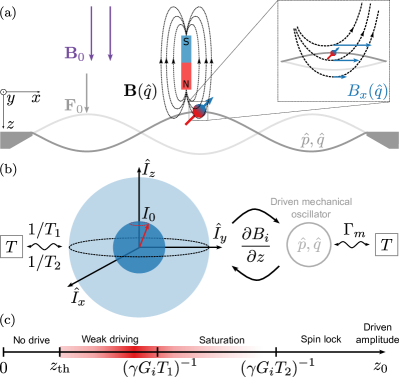
Figure 1: (a) Proposed experiment: A spin ensemble is placed on a mechanical resonator moving within an inhomogeneous magnetic field generated by a nanoscale magnet. By driving the resonator, the spins experience an oscillating magnetic field $\textbf{B}(\hat{q})$ with a component $B_{x}$ (inset). The spins act back on the resonator, producing a force that can be detected as a shift in the resonator frequency. (b) We model the system as a spin ensemble (equilibrium polarization $I_{\parallel}=I_{0}$) interacting with a harmonic oscillator. Both spin ensemble and resonator are coupled to independent baths at temperature $T$, causing spin dephasing and decay with rates $1/T_{2}$ and $1/T_{1}$, respectively, and resonator damping at a rate $\Gamma_{m}$. (c) Illustration of the typical spin regimes according to driven mechanical amplitudes $z_{0}$. Here $z_{\mathrm{th}}$ denotes the thermal motional amplitude. The regime addressed in this work is highlighted in red.

In this work, we propose a protocol for nuclear spin detection based on the near-resonant interaction between a mechanical resonator and an ensemble of nuclear spins. In contrast to earlier ideas [26, 27], our method is most efficient when the resonator is detuned from the spin Larmor frequency. The coupling then causes a shift of the mechanical resonance frequency which can be measured to quantify the spin states. Importantly, in contrast to the driven amplitude predicted in Ref. [26], the response time to the frequency shift is not limited by the ringdown time. Our proposal suits the typical frequency range of strained resonators ($1-$50\text{\,}\mathrm{MHz}$$), but can also be applied to other state-of-the-art systems, such as graphene or carbon nanotube resonators ($\gtrsim$100\text{\,}\mathrm{MHz}$$). Our approach offers a radically simplified experimental apparatus, as it circumvents the need for spin inversion pulses and the related hardware. We also show that for realistic parameters, our method can attain single nuclear spin sensitivity, which would be a major milestone on the way towards spin-based quantum devices. Finally, it opens up a new field of spin manipulation via mechanical driving, drawing parallels to techniques used in cavity optomechanics [10, 28, 29, 30].

We consider a nuclear spin ensemble placed on a mechanical resonator, see Fig. 1(a). The ensemble comprises $N$ spins that interact with a normal mode of the resonator. The composite system can be described with the Zeeman-like Hamiltonian

$$\mathcal{H}=-\hbar\gamma\hat{\textbf{I}}\cdot\textbf{B}+\mathcal{H}_{m},$$ (1)

where $\hbar$ is the reduced Planck constant, $\gamma$ the nuclear spin’s gyromagnetic ratio, and B the magnetic field at the spins’ location. The spin ensemble operator has the three components $\hat{I}_{i}=\sum_{k=1}^{N}\hat{\sigma}_{i,k}/2$ with the spin-$\frac{1}{2}$ Pauli matrices $\hat{\sigma}_{i,k}$ for spin $k=\{1,\cdots,N\}$, and $i\in[x,y,z]$. We describe a single vibrational mode as a driven harmonic oscillator displacing along the $z$ axis governed by the Hamiltonian

$$\mathcal{H}_{m}=\frac{\hat{p}^{2}}{2m}+\frac{1}{2}m\omega_{\mathrm{0}}^{2}\hat{q}^{2}-F_{0}\hat{q}\cos(\omega_{\mathrm{d}}t),$$ (2)

where $\hat{q}$ is the $z$-position operator of the resonator at the position of the spin ensemble, $\hat{p}$ is the corresponding momentum operator, $m$ is the effective mass, $\omega_{\mathrm{0}}$ is the resonance frequency, and $\omega_{\mathrm{d}}$ and $F_{0}$ are the frequency and strength of an applied force, respectively. If B is inhomogeneous, the spins experience a position-dependent field $\textbf{B}(\hat{q})$ as the mechanical resonator vibrates. To lowest order, we approximate this field as $\textbf{B}(\hat{q})\approx\textbf{B}_{0}+\textbf{G}\hat{q}$ with a constant component $\textbf{B}_{0}=\textbf{B}(\hat{q}=0)$ and relevant field gradients $G_{i}=\partial B_{i}/\partial z$. The coherent spin-resonator dynamics therefore obey the Hamiltonian

$$\mathcal{H}\approx-\hbar\omega_{\mathrm{L}}\hat{I}_{z}-\hbar\gamma\hat{q}\textbf{G}\cdot\hat{\textbf{I}}+\mathcal{H}_{m},$$ (3)

with the Larmor precession frequency $\omega_{\mathrm{L}}=\gamma|B_{0}|$.

Any real system, in equilibrium with a thermal bath, experiences mechanical damping (rate $\Gamma_{\mathrm{m}}$), spin decay (longitudinal relaxation time $T_{1}$), and spin decoherence (transverse relaxation time $T_{2}$). We thus succinctly represent our system dynamics using the Heisenberg picture’s dissipative equations of motion (EOM). Driving the resonator to an oscillation amplitude $z_{0}$ well above its zero-point fluctuation amplitude $z_{\mathrm{zpf}}=\sqrt{\hbar/(2m\omega_{0})}$, we treat the mechanical resonator classically in the mean-field approximation. This allows us to approximate the averaged operators as the products of their respective averages, e.g. replacing $\braket{\hat{q}\hat{I}_{i}}$ by $\braket{\hat{q}}\braket{\hat{I}_{i}}$. These averages then evolve via time-dependent Bloch equations [31]

$$\ddot{q} =-\omega_{\mathrm{0}}^{2}q-\Gamma_{\mathrm{m}}\dot{q}+\frac{F_{0}}{m}\cos(\omega_{\mathrm{d}}t)+\frac{\hbar\gamma}{m}\textbf{G}\cdot\textbf{I},$$ (4)

$$\dot{I}_{x,y} =-\frac{1}{T_{2}}I_{x,y}\pm(\omega_{\mathrm{L}}+\gamma qG_{z})I_{y,x}\mp\gamma qG_{y,x}I_{z},$$ (5)

$$\dot{I}_{z} =\frac{1}{T_{1}}\left(I_{0}-I_{z}\right)-\gamma q\left(G_{x}I_{y}-G_{y}I_{x}\right),$$ (6)

where we dropped the $\left<...\right>$ and the hat notation. Here, $I_{0}$ denotes the Boltzmann polarization. In the limit $k_{B}T\gg\hbar\omega_{\mathrm{L}}$, it simplifies to $I_{0}\approx N\hbar\omega_{\mathrm{L}}/(4k_{B}T)$ [32]. The thermomechanical fluctuations do not impact the average resonator’s position $q$, leaving Eq. (4) explicitly independent of temperature $T$. Note that in our simplified model, the spins’ decay (decoherence) time $T_{1}$ ($T_{2}$) is independent of temperature and magnetic field.

To simplify the treatment, we restrict ourselves to the regime where (i) the spins’ force on the resonator is weak compared to the driving force, $|\delta F|\ll F_{0}$, and (ii) the spin-resonator coupling, parameterized by a Rabi frequency $\Omega_{R}=\gamma G_{i}z_{0}$, is weaker than dissipation, meaning $\Omega_{R}\ll 1/T_{2},1/T_{1}$, see Fig. 1(c). In order to fulfill (ii), we select $z_{0}$ to be small and on the order of the thermal motion $z_{\mathrm{th}}$ [31]. The conditions (i) and (ii) imply that we remain in the weak coupling limit, where the oscillation inside the field gradient G excites a precessing spin polarization orthogonal to $\textbf{B}_{0}$ (i.e., $I_{x,y}\neq 0$), but does not lock the spins to the resonator frequency $\omega_{0}$. The backaction of the spins can be treated as a perturbation of the driven resonator oscillation at frequency $\omega_{\mathrm{d}}$. Note that, in the absence of spin locking, spin-spin interactions will lead to short $T_{2}$ times on the order of $100\text{\,}\mathrm{\SIUnitSymbolMicro s}$ for dense spin ensembles [15].

The spin components $I_{x,y}$ exert a linear force back onto the resonator that we calculate via the Harmonic Balance method [3, 5] as detailed in [31]. The force involves a static component $\delta F_{0}=\hbar\gamma I_{0}G_{z}/m$ that shifts the mechanical equilibrium, and two oscillating components, in-phase and quadrature. This dynamical backaction loop causes a frequency shift $\delta\omega$ (corresponding to a phase shift in the driven response) and a linewidth change $\delta\Gamma_{\mathrm{m}}$ [31]:

$$\delta\omega =-g^{2}\left(\frac{\omega_{+}}{\omega_{+}^{2}+1/T_{2}^{2}}+\frac{\omega_{-}}{\omega_{-}^{2}+1/T_{2}^{2}}\right),$$ (7)

$$\delta\Gamma_{\mathrm{m}} =-g^{2}\left(\frac{1/T_{2}}{\omega_{+}^{2}+1/T_{2}^{2}}-\frac{1/T_{2}}{\omega_{-}^{2}+1/T_{2}^{2}}\right),$$ (8)

where $\omega_{\pm}=\omega_{\mathrm{L}}\pm\omega_{\mathrm{d}}$ and $g^{2}=\hbar\gamma^{2}I_{0}\left(G_{x}^{2}+G_{y}^{2}\right)/(4m\omega_{\mathrm{d}})$.

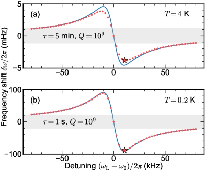
Figure 2: Frequency shift $\delta\omega$ of a string resonator [12] calculated as a function of the detuning between the Larmor frequency $\omega_{\mathrm{L}}$ and the mechanical frequency $\omega_{\mathrm{0}}$. Analytical and numerical results are shown for temperatures of (a) $4\text{\,}\mathrm{K}$ and (b) $0.2\text{\,}\mathrm{K}$. Blue lines correspond to Eq. (7), while red dots are calculated with an explicit Runge-Kutta method of order 8 [17]. A maximal frequency shift in each case is shown by a red star. The shaded area represents the thermal frequency noise standard deviation for an integration time $\tau$ [37, 38]. Common simulated parameters are $\omega_{\mathrm{d}}=\omega_{\mathrm{0}}=2\pi\times$5.5\text{\,}\mathrm{MHz}$$, $G_{x}=G_{y}=$2\text{\,}\mathrm{M}\mathrm{T}\mathrm{/}\mathrm{m}$$, $G_{z}=$1\text{\,}\mathrm{M}\mathrm{T}\mathrm{/}\mathrm{m}$$, $m=$2\text{\,}\mathrm{pg}$$ and $N=10^{6}$. See Table 1 for all device details.

The results in Eq. (7) and in Fig. 2 demonstrate that the equilibrium spin population $I_{0}$ alters the resonator properties through dynamical back-action: the force produced by the oscillating in-plane components $I_{x}$ and $I_{y}$ is delayed with respect to the drive. The force is most pronounced when spins interact with the resonator faster than the resonator’s reaction time ($\Gamma_{m}\ll 1/T_{2},1/T_{1}$). This spin-mediated delayed force creates a closed feedback loop that modifies the resonator’s stiffness (frequency) and enhances or suppresses damping, depending on when the force peaks in relation to position or velocity. Importantly, the strongest spin-mechanics interaction occurs at a detuning $\omega_{\mathrm{L}}\neq\omega_{\mathrm{0}}$ that depends on $1/T_{2}$ and $\omega_{\mathrm{L}}$, see Eq. (7). This is different from the early MRFM proposal that considered resonant coupling forces where $\omega_{\mathrm{L}}=\omega_{\mathrm{0}}$ [26], and from spin noise measurements in MRI [39, 40]. Instead, the effect we rely on resembles dynamical back-action in e.g. cavity optomechanics [41, 10].

For our spin sensing protocol, measuring the frequency shift $\delta\omega$ is advantageous over measuring the linewidth broadening $\delta\Gamma_{\mathrm{m}}$, as the frequency response rate is not intrinsically limited by the ringdown time [42]. In Fig. 2, we show the analytical $\delta\omega$ for a string resonator as a blue line, see “SiN string” entry in Table 1 for details [12]. We consider a sample of $N=10^{6}$ nuclear ¹H spins (gyromagnetic ratio $\gamma=2\pi\times$42.58\text{\,}\mathrm{M}\mathrm{Hz}\mathrm{/}\mathrm{T}$$). The gradient of the magnetic field is calculated from a magnetic tip simulation [31], and we use $T_{2}=$100\text{\,}\mathrm{\SIUnitSymbolMicro s}$$ [15]. In this configuration, simulations indicate a maximum frequency shift of approximately $|\delta\omega_{\text{max}}|/2\pi=$5\text{\,}\mathrm{m}\mathrm{H}\mathrm{z}$$ at a detuning of $(\omega_{\mathrm{L}}-\omega_{0})/2\pi\approx$10\text{\,}\mathrm{k}\mathrm{H}\mathrm{z}$$ at $T=$4\text{\,}\mathrm{K}$$. The analytical frequency shift increases twenty-fold to $|\delta\omega_{\text{max}}|/2\pi\approx$100\text{\,}\mathrm{m}\mathrm{H}\mathrm{z}$$ when the temperature is lowered to $T=$0.2\text{\,}\mathrm{K}$$ because of the higher Boltzmann polarization. To substantiate our analytical result in Eq. (7), we perform a numerical simulation of Eqs. (4)-(6). The simulation closely aligns with the expected results but overestimates the value of $|\delta\omega_{\text{max}}|$ at $4\text{\,}\mathrm{K}$, as seen in Fig. 2(a). The excellent agreement at a lower temperature in Fig. 2(b) suggests that deviations arise from the strain on the assumption $\Omega_{R}\ll 1/T_{2},1/T_{1}$ for fixed spin lifetime $T_{1}$, as $\Omega_{R}\propto z_{0}$ increases with thermal motion [31].

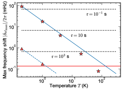
Figure 3: Absolute maximal frequency shift $|\delta\omega_{\mathrm{max}}|$ vs temperature for the string resonator reported in Table 1 (red stars) [12]. Predictions for $10^{4}$ spins are shown as red triangles. The standard deviation of the thermal frequency noise is displayed for different integration times $\tau$ as black dashed lines, setting the minimum threshold for frequency estimation. The blue lines show the analytical frequency shift for $10^{6}$ spins (solid) and $10^{4}$ spins (dashed). The red line indicates the signal that would arise from a single spin. The required averaging time to resolve it is $\tau\sim 2.5\times 10^{4}$ s.

Table 1: Reference resonator parameters. Parameters are estimated or extrapolated from indicated references. Common parameters are $N=10^{6}$ spins, $T_{2}=$100\text{\,}\mathrm{\SIUnitSymbolMicro s}$$, $T_{1}=$50\text{\,}\mathrm{ms}$$ and resonant driving of the resonator $\omega_{\mathrm{d}}=\omega_{\mathrm{0}}$.

Parameters	Symbol	SiN membrane [9]	SiN string [12]	graphene sheet [13]
Effective mass (kg)	$m$	$5\times 10^{-12}$	$2\times 10^{-15}$	$10^{-17}$
Mechanical frequency (MHz)	$\omega_{0}/2\pi$	$1.4$	$5.5$	$46$
Spring constant (N/m)	$k$	387	2.4	0.8
Quality factor (low temperature)	$Q/10^{6}$	$1000$	$1000$	$0.2$
Gradients (MT/m)	$G_{x,y}$, $G_{z}$	$2$, $1$	$2$, $1$	$2$, $1$
Driven amplitude (pm)	$z_{0}$	10	1	2
Thermal motion (pm)	$z_{\mathrm{th}}$	0.08	1	1.8
Rabi frequency (Hz)	$\Omega_{R}/2\pi$	$850$	$85$	$170$
Temperature (K)	$T$	0.2	0.2	0.2
Maximum shift (mHz)	$|\delta\omega_{\mathrm{max}}|/2\pi$	$\mathbf{0.022}$	$\mathbf{90}$	$\mathbf{15500}$

To assess the performance of our spin detection scheme, we calculate numerical frequency shifts for various device geometries (Table 1), showcasing the versatility of the method. The frequency shift notably increases with a decrease in the resonator’s mass, for example graphene sheet resonators are expected to achieve significant frequency shifts exceeding $|\delta\omega_{\text{max}}|/2\pi=$15.5\text{\,}\mathrm{k}\mathrm{H}\mathrm{z}$$. Note that the $1/\omega_{\mathrm{d}}$ dependence of $g^{2}$ in Eqs. (7) and (8) is compensated by $I_{0}\propto\omega_{\mathrm{L}}$.

We systematically collect in Fig. 3 the maximum frequency shift as a function of temperature for string resonators, and compare it with the expected thermal frequency noise [12]. We find that the protocol should allow the detection of $10^{6}$ nuclear spins (¹H) at $4\text{\,}\mathrm{K}$ within less than a minute of averaging under ideal conditions. At moderate dilution refrigeration temperatures of $0.2\text{\,}\mathrm{K}$, the same measurement should be feasible within less than $100\text{\,}\mathrm{ms}$. We should consider two limitations under realistic conditions: first, technical frequency noise stemming from e.g. temperature drifts will increase the frequency fluctuations. Second, inhomogeneous spectral broadening (a distribution in $\omega_{\mathrm{L}}$) of a spin ensemble can reduce the signal, which we discuss in the supplemental material [31].

The theory results summarized in Fig. 3 demonstrate the advances that are feasible in force-detected nanoscale MRI when considering only Boltzmann (thermal) polarization. This polarization is very small for the relevant temperatures and Larmor frequencies; for instance, at $4\text{\,}\mathrm{K}$ and $\omega_{\mathrm{L}}/2\pi=$5.5\text{\,}\mathrm{MHz}$$ (corresponding to $|B_{0}|=$130\text{\,}\mathrm{mT}$$), the effective mean ensemble polarization of a sample containing $10^{6}$ ¹H spins is equivalent to that of 33 fully polarized ¹H spins [31]. While the detection of a single electron spin with a silicon cantilever required an averaging time of roughly $4.7\text{\times}{10}^{4}\text{\,}\mathrm{s}$ in 2004 [44], our method offers the sensitivity for detecting a single nuclear spin (with a roughly $1500$ times lower magnetic moment) in $2.5\text{\times}{10}^{4}\text{\,}\mathrm{s}$. A horizontal red line in Fig. 3 is the corresponding frequency shift for the string device considered here.

The sensitivity of MRI at the nanoscale can be boosted by targeting the statistical spin polarization [16], whose standard deviation surpasses the mean polarization for small ensembles [46]. From simple considerations, we indeed expect that spin-mediated resonator backaction can be extended to the statistical regime. There, instead of a static frequency shift as in Eq. (7), fluctuating nuclear polarization will generate a fluctuating resonator frequency that can be accurately monitored using a phase-locked loop. However, a full model for this regime, based on higher momenta analysis of spin and resonator quantum statistical distributions, [47], is left for future work.

Our method uses a single drive (e.g. via electrical or optomechanical coupling) acting directly on the resonator to detect nuclear spins. It thereby significantly reduces the experimental overhead compared to typical MRFM experiments, which require a microstrip close by the resonator [48] to generate periodic spin flipping through radio-frequency pulses [3]. Dynamic nuclear polarization (DNP) can in principle be implemented to further increase the signal-to-noise ratio [49, 50], potentially allowing the detection of a single nuclear spin within minutes of averaging time. Near-resonant spin-mechanics coupling even opens the possibility of coherently manipulating nuclear spins through mechanical driving [51]. For instance, mechanical vibrations can be harnessed to tilt the ensemble spin polarization fully into the $x$-$y$ plane, resulting in a large increase in the measured signal. Moreover, an intriguing possibility arises when swapping the roles of the resonator and the spin ensemble for spin cooling through backaction [52], akin to cavity cooling in the reversed dissipation regime in cavity optomechanics [53, 54]. Our simplified study paves the way for delving into the intricacies of local spin dissipation and decoherence [55] and dipole-dipole interactions [56] in particular experimental configurations. It also lays the groundwork for exploring further opportunities of parametric driving [23] and multimode resonators [57, 58, 59]. With these capabilities, nanoscale MRI will become a versatile platform for nuclear spin quantum sensing and control on the atomic scale.

Supplemental Material: Near-resonant nuclear spin detection with high-frequency mechanical resonators

S1 Analytical approach

S1.1 Master equation formalism

We offer further details on the analytical solution for the spin-mechanical model introduced in the main text. The model features a driven mechanical resonator moving along $z$, influencing an ensemble of $N$ spins. The spins interact also with a spatially-dependent magnetic field. The combined dynamics is described by the Hamiltonian

$$\mathcal{H}=\frac{\hat{p}^{2}}{2m}+\frac{1}{2}m\omega_{\mathrm{0}}^{2}\hat{q}^{2}-F_{0}\hat{q}\cos(\omega_{\mathrm{d}}t)-\hbar\omega_{\mathrm{L}}\hat{I}_{z}-\hbar\gamma\hat{q}\left(G_{x}\hat{I}_{x}+G_{y}\hat{I}_{y}+G_{z}\hat{I}_{z}\right),$$ (S1)

where $\hbar$ is the reduced Planck constant, $\omega_{\mathrm{0}}$ ($\omega_{\mathrm{L}}$) is the mechanical (Larmor) resonance frequency, $\omega_{\mathrm{d}}$ is the driving frequency, $G_{i}$ is the magnetic gradient along $i\in[x,y,z]$, $\gamma$ is the gyromagnetic ratio of a nuclear spin, and $F_{0}$ is the driving force. Here $\hat{q}$ and $\hat{p}$ stand for the position and momentum operators for the resonator. The spins are described by the collective spin operators $\hat{I}_{i}=\sum_{k=1}^{N}\hat{\sigma}_{i,k}/2$, where $\hat{\sigma}_{i,k}$ are the Pauli matrices describing a spin-$\frac{1}{2}$.

We extract the dissipative equations of motion (EOM) using the Heisenberg picture. We account for mechanical damping ($\Gamma_{\mathrm{m}}$) as well as spin decay ($T_{1}$) and decoherence ($T_{2}$). In order to get physically measurable quantities, we take the mean value of the derived EOM, these are given by:

$$\left<\ddot{\hat{q}}\right> =-\omega_{\mathrm{0}}^{2}\left<\hat{q}\right>-\Gamma_{\mathrm{m}}\left<\dot{q}\right>+\frac{F_{0}}{m}\cos(\omega_{\mathrm{d}}t)+\frac{\hbar\gamma}{m}\left(G_{x}\left<\hat{I}_{x}\right>+G_{y}\left<\hat{I}_{y}\right>+G_{z}\left<\hat{I}_{z}\right>\right),$$ (S2)

$$\left<\dot{\hat{I}}_{x,y}\right> =-\frac{1}{T_{2}}\left<\hat{I}_{x,y}\right>\pm\omega_{\mathrm{L}}\left<\hat{I}_{y,x}\right>\pm\gamma G_{z}\left<\hat{q}\hat{I}_{y,x}\right>\mp\gamma G_{y,x}\left<\hat{q}\hat{I}_{z}\right>,$$ (S3)

$$\left<\dot{\hat{I}}_{z}\right> =\frac{1}{T_{1}}\left(I_{0}-\left<\hat{I}_{z}\right>\right)-\gamma G_{x}\left<\hat{q}\hat{I}_{y}\right>+\gamma G_{y}\left<\hat{q}\hat{I}_{x}\right>,$$ (S4)

where we identify the renormalized mechanical frequency as $\omega_{\mathrm{0}}\mapsto\sqrt{\omega_{0}^{2}+\Gamma_{m}^{2}/4}$. Here $I_{0}$ stands for the Boltzmann (thermal) equilibrium polarization [1]

$$I_{0}=-N\left[(2I+1)\coth\left((2I+1)\hbar\omega_{\mathrm{L}}/(2k_{B}T)\right)-\coth(\hbar\omega_{\mathrm{L}}/(2k_{B}T))\right]/2,$$ (S5)

with $N$ the number of spins in the considered ensemble and $I=\frac{1}{2}$ the spin number.

The resonator motion is driven well above its zero-point fluctuation, we can therfore apply the mean-field approximation and study the semiclassical limit. This entails separating the cross-correlated mean values, i.e. $\left<\hat{q}\hat{I}_{i}\right>=\left<\hat{q}\right>\left<\hat{I}_{i}\right>$. We furthermore drop the braket and hat notation, e.g. $\left<\hat{I}_{x}\right>\equiv I_{x}$, leading to the EOM presented in the main text Eqs. (4)-(6), namely,

$$\ddot{q} =-\omega_{\mathrm{0}}^{2}q-\Gamma_{\mathrm{m}}\dot{q}+\frac{F_{0}}{m}\cos(\omega_{\mathrm{d}}t)+\frac{\hbar\gamma}{m}\textbf{G}\cdot\textbf{I},$$ (S6)

$$\dot{I}_{x,y} =-\frac{1}{T_{2}}I_{x,y}\pm(\omega_{\mathrm{L}}+\gamma qG_{z})I_{y,x}\mp\gamma qG_{y,x}I_{z},$$ (S7)

$$\dot{I}_{z} =\frac{1}{T_{1}}\left(I_{0}-I_{z}\right)-\gamma q\left(G_{x}I_{y}-G_{y}I_{x}\right),$$ (S8)

with vectors $\textbf{G}=(G_{x},G_{y},G_{z})$ and $\textbf{I}=(I_{x},I_{y},I_{z})$.

S1.2 Slow-flow equations of motion

We further analyze here the solution to the main text Eqs. (4)-(6). We assume that the resonator dynamic is dominated by the external force. Thus, the coupling to the spins act as a small correction. We can then write the mechanical motion as $q(t)=q^{(0)}(t)+\delta q(t)$, where $q^{(0)}(t)=u_{q}^{(0)}\cos(\omega_{\mathrm{d}}t)+v_{q}^{(0)}\sin(\omega_{\mathrm{d}}t)$ with

$$u_{q}^{(0)}= \frac{F_{0}}{m\left[\left(\omega_{\mathrm{0}}^{2}-\omega_{\mathrm{d}}^{2}\right)^{2}+\omega_{\mathrm{d}}^{2}\Gamma_{\mathrm{m}}^{2}\right]}\left(\omega_{\mathrm{0}}^{2}-\omega_{\mathrm{d}}^{2}\right),$$ (S9)

$$v_{q}^{(0)}= \frac{F_{0}}{m\left[\left(\omega_{\mathrm{0}}^{2}-\omega_{\mathrm{d}}^{2}\right)^{2}+\omega_{\mathrm{d}}^{2}\Gamma_{\mathrm{m}}^{2}\right]}\omega_{\mathrm{d}}\Gamma_{m}.$$ (S10)

The part accounting for the spins then obeys

$$\ddot{\delta q}=-\omega_{0}^{2}\delta q-\Gamma_{m}\dot{\delta q}+\frac{\hbar\gamma}{m}\textbf{G}\cdot\textbf{I}.$$ (S11)

We express the solution for $\delta q(t)$ in terms of an ansatz

$$\delta q(t)=\delta a_{q}(t)+\delta u_{q}(t)\cos(\omega_{\mathrm{d}}t)+\delta v_{q}(t)\sin(\omega_{\mathrm{d}}t),$$ (S12)

where $\delta a_{q}(t)$, $\delta u_{q}(t)$ and $\delta v_{q}(t)$ are real time-dependent amplitudes to be found. Employing this form of the solution is particularly beneficial when examining perturbations associated with the behavior of a driven harmonic oscillator. The dynamics of the spins in response to the mechanical motion can be calculated employing a similar ansatz

$$I_{i}(t)=a_{i}(t)+u_{i}(t)\cos(\omega_{\mathrm{d}}t)+v_{i}(t)\sin(\omega_{\mathrm{d}}t),$$ (S13)

with amplitudes $a_{i}(t),u_{i}(t),v_{i}(t)$. Given Eq. (S13), the spins exert a time-dependent force on the resonator given by

$$\delta F(t)=\hbar\gamma\textbf{G}\cdot\textbf{I}(t)=\hbar\gamma\left[\mathbf{G}\cdot\mathbf{a}(t)+\mathbf{G}\cdot\mathbf{u}(t)\cos(\omega_{d}t)+\mathbf{G}\cdot\mathbf{v}(t)\sin(\omega_{d}t)\right],$$ (S14)

where we used vector notation for $a_{x,y,z}(t),u_{x,y,z}(t),v_{x,y,z}(t)$.

At this stage, we have not yet introduced any constraints or approximations in the ansatz amplitudes. However, the calculation of the corrections $\delta a_{q},\delta u_{q},\delta v_{q}$ is greatly facilitated by assuming the weak impact of the spin-dependent force on the resonator. Namely, we assume $\langle\langle|\hbar\gamma\textbf{G}\cdot\textbf{I}|\rangle\rangle_{T_{d}}\ll F_{0}$, where $\langle\langle...\rangle\rangle_{T_{d}}$ denotes the average over a drive period $T_{\mathrm{d}}=2\pi/\omega_{\mathrm{d}}$. In this setting, we can assume the amplitudes $\delta a_{q}(t),\delta u_{q}(t),\delta v_{q}(t)$ with respect to $T_{\mathrm{d}}$, accounting for the transient evolution of the amplitude and phase of the resonator towards the steady state [2].

In the steady state, resonator and spin precession amplitudes settle to constant values, i.e. $\delta\dot{a}_{q}=\delta\dot{u}_{q}=\delta\dot{v}_{q}=0$ and $\dot{a}_{i}=\dot{u}_{i}=\dot{v}_{i}=0$. In our ansatz $q(t)$ thus acts as a harmonic magnetic field with frequency $\omega_{\mathrm{d}}$, acting on the spins. In particular, the spin prompts a spin precession component at frequency $\omega_{\mathrm{d}}$, according to Eq. (S13). Note the ansatz does not presuppose the synchronization or “locking” of the spin dynamics with the external field. We seek if such a steady state can exist. To this end, we insert the ansatz for $q(t)$ and $I_{i}(t)$ in the mean-field equations of motion and equate the harmonic amplitudes at both sides of the equations with the same time dependence, a procedure dubbed the “harmonic balance” [3]. This approach also neglects super-harmonic generation (e.g. terms $\cos(2\omega_{\mathrm{d}}t)$, $\sin(2\omega_{\mathrm{d}}t)$) that arises from the mechanical motion driving the spins, which requires extending the harmonic ansatz for $q(t),I_{i}(t)$ to higher frequencies. Note that harmonic balance relies on the slowly-flowing nature of the amplitudes $a_{i},u_{i},v_{i}$ [2].

Linear response theory

The introduction of the ansatz results in nonlinear couplings between the harmonic amplitudes of the mechanical resonator and the spins. The system’s steady states are defined by the roots of these coupled polynomials. While we could solve these equations numerically using advanced algebraic methods, as detailed in reference [4] and implemented in the package [5], we opt for deriving an analytical solution within a linearized framework. Here we find the mechanical dynamics of the resonator in the weakly fluctuating regime $\langle\langle|\delta q|\rangle\rangle_{T_{d}}\ll\langle\langle|q^{(0)}|\rangle\rangle_{T_{d}}$. The smallness of $\delta q$ allows us to neglect the nonlinear coupling between the fluctuations $\delta u_{q}(t),\delta v_{q}(t)$ and the spin amplitudes $a_{i}(t),u_{i}(t),v_{i}(t)$. Under this linearization, the spin dynamics directly follows from the solutions of the first-order differential equations that do not contain $\delta a_{q}(t),\delta u_{q}(t),\delta v_{q}(t)$, namely

$$\dot{a}_{x,y}+1/T_{2}a_{x,y}\mp\omega_{\mathrm{L}}a_{y,x} =0,$$ (S15a)

$$\dot{u}_{x,y}+1/T_{2}u_{x,y}\mp\omega_{\mathrm{L}}u_{y,x}+\omega_{\mathrm{d}}v_{x,y}-\gamma u_{q}^{(0)}(G_{z,x}a_{y,z}-G_{y,z}a_{z,x}) =0,$$ (S15b)

$$\dot{v}_{x,y}+1/T_{2}v_{x,y}\mp\omega_{\mathrm{L}}v_{y,x}-\omega_{\mathrm{d}}u_{x,y}-\gamma v_{q}^{(0)}(G_{z,x}a_{y,z}-G_{y,z}a_{z,x}) =0,$$ (S15c)

$$\dot{a}_{z}+\frac{1}{T_{1}}a_{z}-I_{0}\frac{1}{T_{1}} =0,$$ (S15d)

$$\dot{u}_{z}+\frac{1}{T_{1}}u_{z}+\omega_{\mathrm{d}}v_{z}-\gamma u_{q}^{(0)}(G_{y}a_{x}-G_{x}a_{y}) =0,$$ (S15e)

$$\dot{v}_{z}+\frac{1}{T_{1}}v_{z}-\omega_{\mathrm{d}}u_{z}-\gamma v_{q}^{(0)}(G_{y}a_{x}-G_{x}a_{y}) =0.$$ (S15f)

The resonator features a high quality factor ($\Gamma_{m}\ll 1/T_{2},\frac{1}{T_{1}}$) which, together with the weak spin-resonator coupling ($\gamma G_{i}z_{0}\ll 1/T_{2},\frac{1}{T_{1}}$) lead to spins quickly reaching steady state compared to the slower resonator timescale. This condition permits the application of approximation methods, like adiabatic elimination of the spins [6], in order to approximate the time evolution of the resonator towards its steady state. Our focus is nevertheless on the global steady state behavior, where all amplitudes in the problem are fixed. Solving Eqs. (S15) when $\dot{a}_{i}=\dot{u}_{i}=\dot{v}_{i}=0$ to find the steady state amplitudes $\textbf{a}|_{t\rightarrow\infty},\textbf{u}|_{t\rightarrow\infty},\textbf{v}|_{t\rightarrow\infty}$ leads to a steady state force

$$\delta F|_{t\rightarrow\infty}\approx\hbar\gamma\left[\mathbf{G}\cdot\mathbf{a}|_{t\rightarrow\infty}+\mathbf{G}\cdot\mathbf{u}_{t\rightarrow\infty}\cos(\omega_{d}t)+\mathbf{G}\cdot\mathbf{v}_{t\rightarrow\infty}\sin(\omega_{d}t)\right].$$ (S16)

Such force (S16) will not be in phase with the external resonator’s driving (its quadratures will not be aligned with the drive), namely $u_{q}^{(0)}$, $v_{q}^{(0)}$. To facilitate the expressions, we choose a phase/time origin for the driven resonator (i.e. we perform a gauge fixing), such that $v_{q}^{(0)}=0$ and $u_{q}^{(0)}=F_{0}/(m\sqrt{\left(\omega_{\mathrm{0}}^{2}-\omega_{\mathrm{d}}^{2}\right)^{2}+\omega_{\mathrm{d}}^{2}\Gamma_{\mathrm{m}}^{2}})$. In this gauge, we can identify $\delta F|_{t\rightarrow\infty}\approx\delta F_{0}-\delta\Gamma_{\mathrm{m}}\dot{q}-\delta\Omega^{2}q$, where $\delta F_{0}=\hbar\gamma I_{0}G_{z}/m$ and

$$\delta\Gamma_{\mathrm{m}} =\frac{\hbar\gamma^{2}I_{0}\left(G_{x}^{2}+G_{y}^{2}\right)}{m}\frac{\omega_{\mathrm{L}}T_{2}^{-1}}{\left(T_{2}^{-2}+\omega_{\mathrm{d}}^{2}\right)^{2}+2\left(T_{2}^{-1}-\omega_{\mathrm{d}}\right)\left(T_{2}^{-1}+\omega_{\mathrm{d}}\right)\omega_{\mathrm{L}}^{2}+\omega_{\mathrm{L}}^{4}},$$ (S17)

$$\delta\Omega^{2} =-\frac{\hbar\gamma^{2}I_{0}\left(G_{x}^{2}+G_{y}^{2}\right)}{m}\frac{\omega_{\mathrm{L}}\left(T_{2}^{-2}-\omega_{\mathrm{d}}^{2}+\omega_{\mathrm{L}}^{2}\right)}{\left(T_{2}^{-2}+\omega_{\mathrm{d}}^{2}\right)^{2}+2\left(T_{2}^{-1}-\omega_{\mathrm{d}}\right)\left(T_{2}^{-1}+\omega_{\mathrm{d}}\right)\omega_{\mathrm{L}}^{2}+\omega_{\mathrm{L}}^{4}}.$$ (S18)

We can now reconstruct the mechanical evolution in the steady state from the effective equation of motion. Under resonant driving $\omega_{\mathrm{d}}=\omega_{\mathrm{0}}$,

$$\ddot{q}+\left(\Gamma_{\mathrm{m}}+\delta\Gamma_{\mathrm{m}}\right)\dot{q}+\left(\omega_{\mathrm{0}}+\delta\omega\right)^{2}q|_{t\rightarrow\infty}=F_{0}\cos(\omega_{\mathrm{d}}t)+\delta F_{0},$$ (S19)

with $\delta\omega=\frac{1}{2}\frac{\delta\Omega^{2}}{\omega_{\mathrm{d}}}$. We can rewrite $\delta\Gamma_{\mathrm{m}}$ and $\delta\omega$ in a more convenient way leading to main text Eqs. (7) and (8)

$$\delta\omega=-g^{2}\left(\frac{\omega_{\mathrm{L}}+\omega_{\mathrm{d}}}{1/T_{2}^{2}+\left(\omega_{\mathrm{L}}+\omega_{\mathrm{d}}\right)^{2}}+\frac{\omega_{\mathrm{L}}-\omega_{\mathrm{d}}}{1/T_{2}^{2}+\left(\omega_{\mathrm{L}}-\omega_{\mathrm{d}}\right)^{2}}\right),$$ (S20)

$$\delta\Gamma_{\mathrm{m}}=-g^{2}\left(\frac{T_{2}^{-1}}{1/T_{2}+\left(\omega_{\mathrm{L}}+\omega_{\mathrm{d}}\right)^{2}}-\frac{T_{2}^{-1}}{1/T_{2}^{2}+\left(\omega_{\mathrm{L}}-\omega_{\mathrm{d}}\right)^{2}}\right),$$ (S21)

where we introduced $g^{2}=\hbar\gamma^{2}I_{0}\left(G_{x}^{2}+G_{y}^{2}\right)/(4m\omega_{\mathrm{d}})$.

Beyond linear response

For certain parameter regimes, the nonlinearities in Eqs. (S6)-(S8) can lead to complex behavior in the stationary limit $t\rightarrow\infty$, including self-sustained motion, multi-stability, and limit cycles [7, 8]. In particular, the analogy with optomechanics is expected to break down when the Rabi frequency is comparable to the spin dissipation: $\gamma G_{i}z_{0}\sim 1/T_{2},\frac{1}{T_{1}}$. In that case, the spins’ equilibration is not fast enough before they act back on the resonator, and spin-resonator timescales cannot be adiabatically separated. Effectively, the resonator motion then triggers spin-induced nonlinear effects, such as a periodic time modulation of the Larmor frequency due to the $G_{z}$ gradient (see main text Eqs. (4)-(6)), with frequency $\omega_{\mathrm{d}}$. The resonator’s response would then pick up higher frequency components not described by Eq. (S13). While under the linearized theory, the steady state value is time independent and equal to $I_{z}=I_{0}$, we observe the generation of higher order harmonics in the spectrum of $I_{z}$ [Fig. S1]. Note that in our simulations, we do not focus on the regime where higher excitation makes the spin-conservation constraint ($d(\sum_{i}I_{i}^{2})/dt=0$) relevant, which would lead to additional ‘many-wave mixing’.

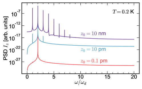
Figure S1: Power spectral density (PSD) of the steady state of a simulated SiN membrane resonator with zero frequency component removed [9] for different driving amplitudes $z_{0}$, $m=$5\text{\times}{10}^{-12}\text{\,}\mathrm{kg}$$, $\omega_{\mathrm{0}}/2\pi=$1.4\text{\,}\mathrm{MHz}$$, $G_{x}=G_{y}=$2\text{\,}\mathrm{M}\mathrm{T}\mathrm{/}\mathrm{m}$$, $G_{z}=$1\text{\,}\mathrm{M}\mathrm{T}\mathrm{/}\mathrm{m}$$, $N=10^{6}$ spins, $T_{2}=$100\text{\,}\mathrm{\SIUnitSymbolMicro s}$$, $T_{1}=$50\text{\,}\mathrm{ms}$$ and resonant driving of the resonator $\omega_{\mathrm{d}}=\omega_{\mathrm{0}}$.

A comprehensive examination of nonlinearities in our detection protocol is beyond the scope of this manuscript; however, we offer a brief overview of the necessary approach below. The impact of weak nonlinearities can be expressed by still expanding the solution for $x(t)$ with an ansatz of the form

$$x(t)=a_{q}(t)+u_{q}(t)\cos(\omega_{\mathrm{d}}t)+v_{q}(t)\sin(\omega_{\mathrm{d}}t),$$ (S22)

which includes both the displacement by the driving field and small fluctuations, while keeping the same ansatz for the spins in Eq. (S13). We will account now for the nonlinear corrections to this resonant behavior. The equations of motion for the ansatz amplitudes without linearization read

$$\omega_{0}^{2}a_{q}+\tilde{G}_{x}a_{x}+\tilde{G}_{y}a_{y}+\tilde{G}_{z}a_{z}+\Gamma_{m}\dot{a}_{q}=0,$$ (S23)

$$\omega_{0}^{2}u_{q}-\omega_{\mathrm{d}}^{2}u_{q}+\Gamma_{m}\omega_{\mathrm{d}}v_{q}+2\omega_{\mathrm{d}}\dot{v}_{q}-F_{0}+\tilde{G}_{x}u_{x}+\tilde{G}_{y}u_{y}+\tilde{G}_{z}u_{z}+\Gamma_{m}\dot{u}_{q}=0,$$ (S24)

$$\omega_{0}^{2}v_{q}-\omega_{\mathrm{d}}^{2}v_{q}-2\omega_{\mathrm{d}}\dot{u}_{q}-\Gamma_{m}\omega_{\mathrm{d}}u_{q}\tilde{G}_{x}v_{x}+\tilde{G}_{y}v_{y}+\tilde{G}_{z}v_{z}+\Gamma_{m}\dot{v}_{q}=0,$$ (S25)

$$\frac{1}{T_{2}}a_{x}+\omega_{\mathrm{L}}a_{y}+\tilde{G}_{z}a_{q}a_{y}-\tilde{G}_{y}a_{q}a_{z}-\frac{\tilde{G_{y}}}{2}u_{q}u_{z}+\frac{\tilde{G_{z}}}{2}u_{q}u_{y}+\frac{\tilde{G_{z}}}{2}v_{q}v_{y}-\frac{\tilde{G_{y}}}{2}v_{q}v_{z}+\dot{a}_{x}=0,$$ (S26)

$$\frac{1}{T_{2}}u_{x}+\omega_{\mathrm{L}}u_{y}+\omega_{\mathrm{d}}v_{x}+\tilde{G}_{z}a_{q}u_{y}+\tilde{G}_{z}a_{y}u_{q}-\tilde{G}_{y}a_{q}u_{z}-\tilde{G}_{y}a_{z}u_{q}+\dot{u}_{x}=0,$$ (S27)

$$\frac{1}{T_{2}}v_{x}+\omega_{\mathrm{L}}v_{y}-\omega_{\mathrm{d}}u_{x}+\tilde{G}_{z}a_{q}v_{y}+\tilde{G}_{z}a_{y}v_{q}-\tilde{G}_{y}a_{z}v_{q}-\tilde{G}_{y}a_{q}v_{z}+\dot{v}_{x}=0,$$ (S28)

$$\frac{1}{T_{2}}a_{y}-\omega_{\mathrm{L}}a_{x}+\tilde{G}_{x}a_{q}a_{z}-\tilde{G}_{z}a_{q}a_{x}-\frac{\tilde{G_{z}}}{2}u_{q}u_{x}+\frac{\tilde{G_{x}}}{2}u_{q}u_{z}+\frac{\tilde{G_{x}}}{2}v_{q}v_{z}-\frac{\tilde{G_{z}}}{2}v_{q}v_{x}+\dot{a}_{y}=0,$$ (S29)

$$\frac{1}{T_{2}}u_{y}+\omega_{\mathrm{d}}v_{y}-\omega_{\mathrm{L}}u_{x}+\tilde{G}_{x}a_{q}u_{z}+\tilde{G}_{x}a_{z}u_{q}-\tilde{G}_{z}a_{q}u_{x}-\tilde{G}_{z}a_{x}u_{q}+\dot{u}_{y}=0,$$ (S30)

$$\frac{1}{T_{2}}v_{y}-\omega_{\mathrm{d}}u_{y}+\tilde{G}_{x}a_{z}v_{q}-\omega_{\mathrm{L}}v_{x}+\tilde{G}_{x}a_{q}v_{z}-\tilde{G}_{z}a_{x}v_{q}-\tilde{G}_{z}a_{q}v_{x}+\dot{v}_{y}=0,$$ (S31)

$$\frac{1}{T_{1}}a_{z}-I_{0}\frac{1}{T_{1}}+\tilde{G}_{y}a_{q}a_{x}-\tilde{G}_{x}a_{q}a_{y}+\frac{\tilde{G_{y}}}{2}u_{q}u_{x}-\frac{\tilde{G_{x}}}{2}u_{q}u_{y}-\frac{\tilde{G_{x}}}{2}v_{q}v_{y}+\frac{\tilde{G_{y}}}{2}v_{q}v_{x}+\dot{a}_{z}=0,$$ (S32)

$$\frac{1}{T_{1}}u_{z}+\omega_{\mathrm{d}}v_{z}+\tilde{G}_{y}a_{q}u_{x}+\tilde{G}_{y}a_{x}u_{q}-\tilde{G}_{x}a_{y}u_{q}-\tilde{G}_{x}a_{q}u_{y}+\dot{u}_{z}=0,$$ (S33)

$$\frac{1}{T_{1}}v_{z}-\omega_{\mathrm{d}}u_{z}+\tilde{G}_{y}a_{q}v_{x}+\tilde{G}_{y}a_{x}v_{q}-\tilde{G}_{x}a_{q}v_{y}-\tilde{G}_{x}a_{y}v_{q}+\dot{v}_{z}=0.$$ (S34)

where $\tilde{G}_{i}=\gamma G_{i}$ is shorthand. The resonator’s susceptibility can then by found by (i) finding the steady states of these equations, i.e. finding the roots of a system of coupled polynomials arising from $\dot{a}_{i}=\dot{u}_{i}=\dot{v}_{i}=\dot{a}_{q}=\dot{u}_{q}=\dot{v}_{q}=0$, and (ii) performing linear fluctuation analysis around these solutions. These two steps can be facilitated by the use of the HarmonicBalance.jl package [5].

Finally, the frequency spectrum in Fig. S1 reveals that as the driving strength increases, the lowest order nonlinear effect is the generation of a second harmonic at a frequency $2\omega_{\mathrm{d}}$. Similar equations to Eqs. (S23) can be similarly obtained for the amplitudes of an extended ansatz that includes also the higher harmonic generated at $2\omega_{\mathrm{d}}$.

S1.3 Linewidth change

In Fig. S2, we show the linewidth change predicted by the analytical model for the three resonators considered in this work. This change produces an effective reduction of the resonator’s quality factor, resulting in “cold damping”, as conventionally used in cavity optomechanics [10]. The influence of cold damping on a cantilever in an MRFM experiment, albeit in a nonresonant setting, was studied previously [11].

(a)

(b)

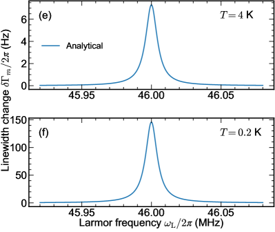
(c)

Figure S2: Linewidth change for (a)-(b) a SiN membrane resonator [9], (c)-(d) a SiN string resonator [12] and (e)-(f) a graphene sheet resonator [13], note the difference in the vertical scale unit.

S2 Relaxation and spectral broadening

S2.1 Relaxation rates

The spin lifetime $T_{1}$ of nuclear spins resulting from energy relaxation can vary strongly in typical nuclear magnetic resonance (NMR) experiments, ranging from microseconds to days. Our experimental situation is untypical, as we will probe nanoscale samples at low temperatures and low magnetic fields. We do not need a very specific value for $T_{1}$, as our analytical results hold as long as $T_{1}\ll 1/\Gamma_{\mathrm{m}}$. To avoid speculation about the dependency of $T_{1}$ on field strength and temperatures below $70\text{\,}\mathrm{K}$, we use the same value of $T_{1}=$50\text{\,}\mathrm{ms}$$ for all our simulations. If needed for specific experimental situation, we envisage reducing $T_{1}$ by introducing paramagnetic agents, such as free radicals or metal ions [14].

S2.2 Decoherence due to spin-spin coupling

In typical NMR experiments, interactions between neighboring nuclear spins can often be neglected when the Rabi frequency $\Omega_{R}$ exceeds the spin-spin coupling strength $J$. In that scenario, the range of Larmor frequencies that are affected by the spin lock is dominated by the spectral “power broadening” equal to $\Omega_{R}$. By contrast, in the experiments we describe, the condition $\Omega_{R}\geq J$ is typically not fulfilled, and we are limited by the condition $\Omega_{R}\ll\frac{1}{T_{2}},\frac{1}{T_{1}}$. As we cannot ignore spin-spin interaction in the weak-driving regime, $J$ is explicitly implemented in the simulations through the spin decoherence time $T_{2}=$100\text{\,}\mathrm{\SIUnitSymbolMicro s}$$ [15].

S2.3 Inhomogeneous broadening

In our paper, we primarily consider the interaction between a mechanical resonator and an ensemble of spins with identical Larmor frequencies. This was done to present the fundamental concept as clearly as possible. However, any real sample is extended in space, and therefore contains spins at various positions within the magnetic field gradient. When all these spins in a sample are excited at the same time, their variation in Larmor frequencies leads to a so-called “inhomogeneous broadening” $1/T_{2}^{*}$ and a corresponding dephasing time $T_{2}^{*}$. For $T_{2}^{*}<T_{2}$, the inhomogeneous broadening dominates over spin-spin interactions and increases the effective spectral with of the ensemble. In our sample, the driving fields are necessarily weak to fulfill the condition $\Omega_{R}=\gamma G_{i}z_{0}\ll 1/T_{2},1/T_{1}$. Only the spins within the narrow range $\omega_{\mathrm{L}}=\omega_{0}\pm\Omega_{R}$ are directly excited, yielding an inhomogeneous broadening of $1/T_{2}^{*}=\Omega_{R}$. Through spin-spin interactions, all the spins within $\omega_{\mathrm{L}}=\omega_{0}\pm 1/T_{2}$ are indirectly excited. As $\Omega_{R}\ll 1/T_{2}$, the broadening of the spin ensembles is limited by $1/T_{2}$, not $1/T_{2}^{*}$. We therefore do not need to be concerned about the effects of inhomogeneous broadening.

S2.4 Signal contributions with different signs

The spectral width of the spins that are excited in our scheme depends on $1/T_{2}$. In principle, this has the consequence that the resonator interacts with spins covering a significant part of the frequencies shown in Fig. 2, which can lead to a mutual cancellation of positive and negative frequency shifts. In the following, we discuss how this problem can be avoided.

• Differential measurements: the contributions from different parts of the sample can cancel each other when they generate frequency shifts with equal strength and opposite signs. However, as the nanomagnetic probe is scanned over the sample, spins at different locations enter the strong field gradient at different scan positions. For instance, at a certain position, mainly spins contributing positive frequency shifts may be located within the strong gradient, causing a strong positive frequency shift. The outcome of a full scan then corresponds to a differential spin signal, where the frequency shift of the resonator does not indicate the number of spins at one particular Larmor frequency, but rather the relative weight between ‘positive’ and ‘negative’ spins. Knowing the field distribution of the nanomagnetic probe (which can be calibrated with well-known samples), the spatial distribution of spins can be reconstructed by integrating over the differential signal.

• Statistical polarization: in MRFM, we typically probe the statistical polarization of a spin ensemble, not the Boltzmann polarization [16]. In this case, only the number of spins (weighted by the square of the local gradient) is important to evaluate the measured signal, not the sign of their individual contributions. For instance, let us assume the simple case of two equal spin sub-ensembles with different Larmor frequencies that contribute with equally strong but opposite frequency shifts in Fig. 2. Assuming the spins fluctuate thermally (and ignoring any remaining Boltzmann polarization), the two ensembles will spend an equal amount of time in a symmetric configuration as in the antisymmetric one. In the antisymmetric configuration, the sub-ensembles will contribute to the frequency shifts with the same sign. The total resonator frequency variance resulting from the combined effect of the two ensembles in the long-time limit is therefore overall increased, not reduced.

• Single spin: One exciting aspect of the method we propose is the quantum limit of probing a single spin. In this situation, the problem arising from variations in the Larmor frequency naturally vanishes, leaving only a well-defined Larmor frequency generating a single frequency shift.

S3 Exact numerical simulations

To verify our theoretical predictions, we numerically simulate our mean-field EOM given by Eqs. (S6)-(S8). We solve the EOM using an explicit Runge-Kutta method of order 8, which is well-suited for handling the large separation of timescales in the problem [17].

S3.1 Results for different devices

We focus on three device families: silicon nitride (SiN) membranes, SiN strings, and graphene sheets. These devices span across a large range of frequencies and across several orders of magnitude of mass. We simulate a hypothetical sample containing $N=10^{6}$ ¹H nuclear spins, corresponding to a sample size of $\approx($20\text{\,}\mathrm{nm}$)^{3}$ [18]. To estimate the magnetic field gradients, we numerically simulate a cobalt nanorod of length $1\text{\,}\mathrm{\SIUnitSymbolMicro m}$ and radius $50\text{\,}\mathrm{nm}$ that is pre-magnetized to $1\text{\,}\mathrm{T}$, inspired by Ref. [19]. The magnetic simulation results are presented in Sect. S3.2. The driving strength, proportional to $z_{0}$, can be easily tuned in the experiment. We choose it in the following such that $\Omega_{R}\ll\frac{1}{T_{2}},\frac{1}{T_{1}}$. Due to the low $T_{2}=$100\text{\,}\mathrm{\SIUnitSymbolMicro s}$$ value, this condition might be hard to fulfill for high temperatures as the driving amplitude $z_{0}$ is lower bound by the resonator’s thermal motion. Membrane and string resonators can have quality factor around $Q=\omega_{\mathrm{0}}/\Gamma_{\mathrm{m}}=10^{8}$ at room temperature and increase up to $10^{9}$ for low temperature $T\leq 4$ K. To fulfill the condition $\Gamma_{\mathrm{m}}\ll 1/T_{2},\frac{1}{T_{1}}$ with these $Q$ factors, $T_{1}$ should be at most in the minute range. However, in order to reduce the number of timesteps required in the simulation, we use a reduced $T_{1}$ time as well as a reduced quality factor $Q$ for the resonator within the regime $\Gamma_{\mathrm{m}}\ll 1/T_{2},\frac{1}{T_{1}}$. Throughout the simulations, we used $T_{1}=$50\text{\,}\mathrm{ms}$$.

Figure S3 shows the analytical (blue lines) and the numerical (red dots) results for a SiN membrane resonator [9]. Figure S3(a) and (b) show the results for the case with driving amplitude close to the thermal motion of the membrane at the given temperature ($T=$4\text{\,}\mathrm{K}$$ for (a) and $T=$0.2\text{\,}\mathrm{K}$$ for (b)). In these cases, the numerical data follows very closely the analytical model as the condition $\Omega_{R}\ll 1/T_{2},\frac{1}{T_{1}}$ is strongly fulfilled. However, the integration time to resolve the frequency shift above the frequency noise is extremely long. On the opposite, Figure S3(c) and (d) show the same case but with increased driving amplitude ($z_{0}=$10\text{\,}\mathrm{pm}$$ for both cases). In this case, $\Omega_{R}$ is still smaller than $1/T_{2}$ but not anymore smaller than $\frac{1}{T_{1}}$ (in our simulations $T_{1}=$50\text{\,}\mathrm{ms}$$). We see that the numerical frequency shift is now smaller than the analytical one, nevertheless, the integration time to resolve the frequency shift is now strongly reduced to feasible values.

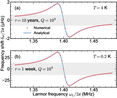
(a)

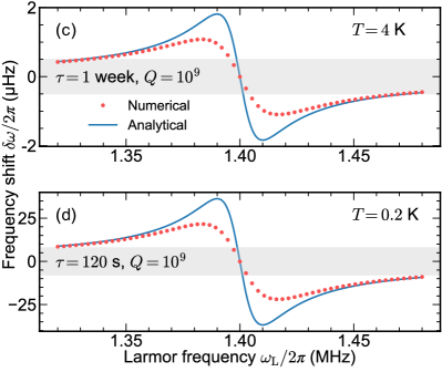
(b)

Figure S3: Exact numerical simulations of a SiN membrane resonator [9], $m=$5\text{\times}{10}^{-12}\text{\,}\mathrm{kg}$$, $\omega_{\mathrm{0}}/2\pi=$1.4\text{\,}\mathrm{MHz}$$. The same resonator is simulated for different temperatures and different driving strengths. For (a) and (b), the drive is chosen at the thermal motion amplitude whereas for (c) and (d) it is chosen to be 2 orders of magnitude above the former. Note the strong decrease in thermal frequency noise in (c) and (d) at the expense of a reduced frequency shift. The drive amplitudes are $z_{0}=$0.4\text{\,}\mathrm{pm}$$ for (a), $z_{0}=$0.08\text{\,}\mathrm{pm}$$ for (b) and $z_{0}=$10\text{\,}\mathrm{pm}$$ for (c) and (d). Common simulated parameters are $G_{x}=G_{y}=$2\text{\,}\mathrm{M}\mathrm{T}\mathrm{/}\mathrm{m}$$, $G_{z}=$1\text{\,}\mathrm{M}\mathrm{T}\mathrm{/}\mathrm{m}$$, $N=10^{6}$ spins, $T_{2}=$100\text{\,}\mathrm{\SIUnitSymbolMicro s}$$, $T_{1}=$50\text{\,}\mathrm{ms}$$ and resonant driving of the resonator $\omega_{\mathrm{d}}=\omega_{\mathrm{0}}$.

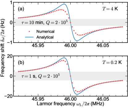
Figure S4: Exact numerical simulations of a graphene sheet resonator [13], $m=10^{-17}$ kg, $\omega_{\mathrm{0}}/2\pi=$46\text{\,}\mathrm{MHz}$$, $z_{0}=$10\text{\,}\mathrm{pm}$$ in the (a) $T=$4\text{\,}\mathrm{K}$$ case and $z_{0}=$2\text{\,}\mathrm{pm}$$ in the (b) $T=$0.2\text{\,}\mathrm{K}$$ case. Common simulated parameters are $G_{x}=G_{y}=$2\text{\,}\mathrm{M}\mathrm{T}\mathrm{/}\mathrm{m}$$, $G_{z}=$1\text{\,}\mathrm{M}\mathrm{T}\mathrm{/}\mathrm{m}$$, $N=10^{6}$ spins, $T_{2}=$100\text{\,}\mathrm{\SIUnitSymbolMicro s}$$, $T_{1}=$50\text{\,}\mathrm{ms}$$ and resonant driving of the resonator $\omega_{\mathrm{d}}=\omega_{\mathrm{0}}$.

From Eq. (S7) we see that the spin dynamics should feature an additional effect that is not described by the analytical model: the jittering of the rotation frequency along the polarization axis ($I_{z}$ in our case) due to the modulation of the Larmor frequency from the $G_{z}$ gradient. The jittering is caused by the second term on the r.h.s. of the equation, which contains a magnetic gradient-dependent contribution. As the oscillator is driven, it is possible to leverage this frequency jittering. For the case of the string resonator presented in the main text, the Larmor frequency is $\omega_{\mathrm{L}}/2\pi=$5.5\text{\,}\mathrm{MHz}$$, the greatest driving strength (at $T=$77\text{\,}\mathrm{K}$$) is $z_{0}=$20\text{\,}\mathrm{pm}$$, and the gradient along $z$ is $G_{z}=$1\text{\,}\mathrm{M}\mathrm{T}\mathrm{/}\mathrm{m}$$ MT/m. The maximum amplitude of the frequency modulation (recall that $q$ oscillates) is $\gamma G_{z}z_{0}/2\pi\sim$1\text{\,}\mathrm{kHz}$$, amounting to $\sim$0.02\text{\,}\mathrm{\char 37\relax}$$ of the precession frequency, so the effect is very limited for this resonator. For the membrane resonator, the greatest driving is $10\text{\,}\mathrm{pm}$, giving a frequency jittering of $\sim$500\text{\,}\mathrm{Hz}$$, amounting here to $\sim$0.04\text{\,}\mathrm{\char 37\relax}$$ of the precession frequency. For the third resonator, the graphene sheet, the effect is even smaller due to the higher Larmor frequency: in this case, the jittering is smaller than $0.001\text{\,}\mathrm{\char 37\relax}$ of the precession frequency. We conclude that this effect can be ignored for the resonators we are considering.

S3.2 Magnetic tip simulations

To extract a meaningful value for the magnetic field gradients $G_{i}$, we perform a numerical simulation of the magnetic field of a cobalt nanomagnet. The nanomagnet resembles a cylinder of length $L=$1\text{\,}\mathrm{\SIUnitSymbolMicro m}$$ and radius $R=$50\text{\,}\mathrm{nm}$$. We are directly inspired by the nanomagnet presented in Ref. [19]. We assume that the nanomagnet is pre-magnetized to $1\text{\,}\mathrm{T}$ and we apply an external magnetic field. The latter is used to tune the region where the Larmor frequency matches the mechanical resonator’s frequency; we want it to be as close as possible to the nanomagnet in order to harvest the highest magnetic field gradients. Hence, the external magnetic field can be in the opposite direction of the nanomagnet $z$-magnetic field depending on the device investigated, as the required magnetic field for frequency matching can be smaller than the nanomagnet-generated magnetic field. The nanomagnet magnetization should remain roughly constant due to the shape anisotropy, which turns our Co cylinder effectively into a hard magnet [19].

Figure S5(a) shows the absolute value of the magnetic field in the vicinity of the nanomagnet (black rectangle) for the case of a SiN string with $\omega_{0}/2\pi=$5.5\text{\,}\mathrm{MHz}$$. In this case, we apply an external magnetic field of $0.2\text{\,}\mathrm{T}$ in the opposite direction of the nanomagnet $z$-magnetic field. The region where the Larmor frequency of the spins would be resonant with the resonator mechanical frequency ($\omega_{\mathrm{L}}=\omega_{\mathrm{0}}$) is showed as a black line. We can then extract the magnetic field gradients in the $x$ and $z$ directions of the spin reference frame. These gradients are displayed on Fig. S5(b) and S5(c). In the optimal case, the sample would be in a region where $G_{x}$ is maximal and $G_{z}$ minimal. In addition, the sample must be small enough so that it does not overlap the right and left lobes otherwise the effect of the $G_{x}$ gradient would cancel out due to the sign inversion of the latter.

From this simulation, we extract the value of the gradients used in the main text, namely $G_{x}=G_{y}=$2\text{\,}\mathrm{M}\mathrm{T}\mathrm{/}\mathrm{m}$$ ($G_{x}=G_{y}$ by symmetry) and $G_{z}=$1\text{\,}\mathrm{M}\mathrm{T}\mathrm{/}\mathrm{m}$$.

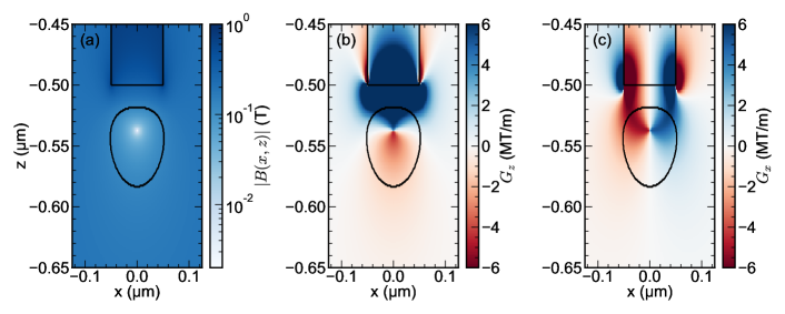
Figure S5: Numerical simulation of a cobalt nanomagnet (black rectangle) pre-magnetized at 1 T subjected to an external magnetic field of $0.2\text{\,}\mathrm{T}$ in the $z$-direction (bottom to top). (a) Absolute value of the magnetic field. The black line shows where the magnetic field is resonant with the mechanical resonator: $\gamma B_{0}=\omega_{\mathrm{L}}=\omega_{\mathrm{0}}=2\pi\times$5.5\text{\,}\mathrm{MHz}$$. The magnetic field gradients are calculated from (a) and result in a $G_{z}$ (b) and a $G_{x}$ (c) component. Note that $G_{x}$ and $G_{z}$ are the magnetic field gradients in the $x$ and $z$ directions of the spin reference frame (and not the nanomagnet reference frame).

S3.3 Boltzmann vs statistical polarization

To justify the interest in looking at the statistical polarization of the spins instead of the Boltzmann polarization, we can easily plot the different values for a range of temperature and number of spins in the sample. The Boltzmann polarization is given by Eq. (S5) whereas the statistical polarization is given by $I_{0}=\frac{1}{2}\sqrt{N}$ [16]. The comparison is shown in Fig. S6 for the string resonator. The black dashed line shows the case of $10^{6}$ spins used in the main text. It is clear that for samples containing fewer spins the statistical polarization would allow a much stronger signal than the Boltzmann polarization in the same conditions.

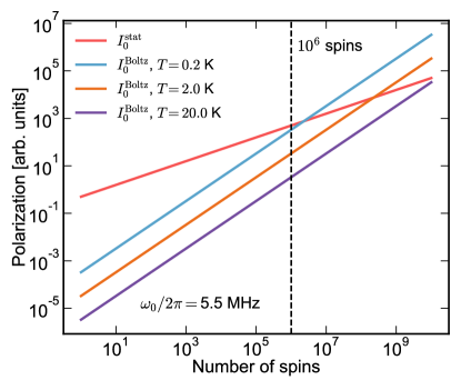
Figure S6: Boltzmann polarization compared to the statistical polarization for different numbers of spins in the sample and different temperatures for the string resonator case. The black dashed line represents a sample of $10^{6}$ spins like the one mainly used throughout the main text.

References

- Sidles [1991] J. A. Sidles, Noninductive detection of single-proton magnetic resonance, Applied Physics Letters 58, 2854 (1991).
- Poggio and Degen [2010] M. Poggio and C. L. Degen, Force-detected nuclear magnetic resonance: recent advances and future challenges, Nanotechnology 21, 342001 (2010).
- Degen et al. [2009] C. L. Degen, M. Poggio, H. J. Mamin, C. T. Rettner, and D. Rugar, Nanoscale magnetic resonance imaging, Proceedings of the National Academy of Sciences 106, 1313 (2009).
- Nichol et al. [2013] J. M. Nichol, T. R. Naibert, E. R. Hemesath, L. J. Lauhon, and R. Budakian, Nanoscale fourier-transform magnetic resonance imaging, Physical Review X 3, 031016 (2013).
- Grob et al. [2019] U. Grob, M. D. Krass, M. Héritier, R. Pachlatko, J. Rhensius, J. Košata, B. A. Moores, H. Takahashi, A. Eichler, and C. L. Degen, Magnetic resonance force microscopy with a one-dimensional resolution of 0.9 nanometers, Nano Letters 19, 7935 (2019).
- Haas et al. [2022] H. Haas, S. Tabatabaei, W. Rose, P. Sahafi, M. Piscitelli, A. Jordan, P. Priyadarsi, N. Singh, B. Yager, P. J. Poole, D. Dalacu, and R. Budakian, Nuclear magnetic resonance diffraction with subangstrom precision, Proceedings of the National Academy of Sciences 119, e2209213119 (2022).
- Eichler [2022] A. Eichler, Ultra-high-q nanomechanical resonators for force sensing, Materials for Quantum Technology 2, 043001 (2022).
- Reinhardt et al. [2016] C. Reinhardt, T. Müller, A. Bourassa, and J. C. Sankey, Ultralow-noise sin trampoline resonators for sensing and optomechanics, Physical Review X 6, 021001 (2016).
- Norte et al. [2016] R. Norte, J. Moura, and S. Gröblacher, Mechanical resonators for quantum optomechanics experiments at room temperature, Physical Review Letters 116, 147202 (2016).
- Tsaturyan et al. [2017] Y. Tsaturyan, A. Barg, E. S. Polzik, and A. Schliesser, Ultracoherent nanomechanical resonators via soft clamping and dissipation dilution, Nature Nanotechnology 12, 776 (2017).
- Rossi et al. [2018] M. Rossi, D. Mason, J. Chen, Y. Tsaturyan, and A. Schliesser, Measurement-based quantum control of mechanical motion, Nature 563, 53 (2018).
- Reetz et al. [2019] C. Reetz, R. Fischer, G. Assumpção, D. McNally, P. Burns, J. Sankey, and C. Regal, Analysis of membrane phononic crystals with wide band gaps and low-mass defects, Physical Review Applied 12, 044027 (2019).
- Ghadimi et al. [2018] A. H. Ghadimi, S. A. Fedorov, N. J. Engelsen, M. J. Bereyhi, R. Schilling, D. J. Wilson, and T. J. Kippenberg, Elastic strain engineering for ultralow mechanical dissipation, Science 360, 764 (2018).
- Beccari et al. [2022] A. Beccari, D. A. Visani, S. A. Fedorov, M. J. Bereyhi, V. Boureau, N. J. Engelsen, and T. J. Kippenberg, Strained crystalline nanomechanical resonators with quality factors above 10 billion, Nature Physics 18, 436 (2022).
- Gisler et al. [2022] T. Gisler, M. Helal, D. Sabonis, U. Grob, M. Héritier, C. L. Degen, A. H. Ghadimi, and A. Eichler, Soft-clamped silicon nitride string resonators at millikelvin temperatures, Physical Review Letters 129, 104301 (2022).
- Bereyhi et al. [2022a] M. J. Bereyhi, A. Arabmoheghi, A. Beccari, S. A. Fedorov, G. Huang, T. J. Kippenberg, and N. J. Engelsen, Perimeter modes of nanomechanical resonators exhibit quality factors exceeding at room temperature, Physical Review X 12, 021036 (2022a).
- Fedorov et al. [2020] S. Fedorov, A. Beccari, N. Engelsen, and T. Kippenberg, Fractal-like mechanical resonators with a soft-clamped fundamental mode, Physical Review Letters 124, 025502 (2020).
- Bereyhi et al. [2022b] M. J. Bereyhi, A. Beccari, R. Groth, S. A. Fedorov, A. Arabmoheghi, T. J. Kippenberg, and N. J. Engelsen, Hierarchical tensile structures with ultralow mechanical dissipation, Nature Communications 13, 3097 (2022b).
- Shin et al. [2021] D. Shin, A. Cupertino, M. H. J. de Jong, P. G. Steeneken, M. A. Bessa, and R. A. Norte, Spiderweb nanomechanical resonators via bayesian optimization: Inspired by nature and guided by machine learning, Advanced Materials 34, 2270019 (2021).
- Moser et al. [2013] J. Moser, J. Güttinger, A. Eichler, M. J. Esplandiu, D. E. Liu, M. I. Dykman, and A. Bachtold, Ultrasensitive force detection with a nanotube mechanical resonator, Nature Nanotechnology 8, 493 (2013).
- Rossi et al. [2016] N. Rossi, F. R. Braakman, D. Cadeddu, D. Vasyukov, G. Tütüncüoglu, A. Fontcuberta i Morral, and M. Poggio, Vectorial scanning force microscopy using a nanowire sensor, Nature Nanotechnology 12, 150 (2016).
- Hälg et al. [2021] D. Hälg, T. Gisler, Y. Tsaturyan, L. Catalini, U. Grob, M.-D. Krass, M. Héritier, H. Mattiat, A.-K. Thamm, R. Schirhagl, E. C. Langman, A. Schliesser, C. L. Degen, and A. Eichler, Membrane-based scanning force microscopy, Physical Review Applied 15, l021001 (2021).
- Košata et al. [2020] J. Košata, O. Zilberberg, C. L. Degen, R. Chitra, and A. Eichler, Spin detection via parametric frequency conversion in a membrane resonator, Physical Review Applied 14, 014042 (2020).
- Aspelmeyer et al. [2014] M. Aspelmeyer, T. J. Kippenberg, and F. Marquardt, Cavity optomechanics, Reviews of Modern Physics 86, 1391 (2014).
- Bachtold et al. [2022] A. Bachtold, J. Moser, and M. I. Dykman, Mesoscopic physics of nanomechanical systems, Rev. Mod. Phys. 94, 045005 (2022).
- Sidles [1992] J. A. Sidles, Folded stern-gerlach experiment as a means for detecting nuclear magnetic resonance in individual nuclei, Physical Review Letters 68, 1124 (1992).
- Berman and Tsifrinovich [2022] G. P. Berman and V. I. Tsifrinovich, Magnetic resonance force microscopy with matching frequencies of cantilever and spin, Journal of Applied Physics 131, 044301 (2022).
- Lee et al. [2016] K. W. Lee, D. Lee, P. Ovartchaiyapong, J. Minguzzi, J. R. Maze, and A. C. Bleszynski Jayich, Strain coupling of a mechanical resonator to a single quantum emitter in diamond, Physical Review Applied 6, 034005 (2016).
- Teissier et al. [2017] J. Teissier, A. Barfuss, and P. Maletinsky, Hybrid continuous dynamical decoupling: a photon-phonon doubly dressed spin, Journal of Optics 19, 044003 (2017).
- MacQuarrie et al. [2013] E. R. MacQuarrie, T. A. Gosavi, N. R. Jungwirth, S. A. Bhave, and G. D. Fuchs, Mechanical spin control of nitrogen-vacancy centers in diamond, Physical Review Letters 111, 227602 (2013).
- [31] See supplemental material at [url will be inserted by publisher] for further details on the analytical approach and additional simulation case studies.
- Niinikoski [2020] T. O. Niinikoski, The Physics of Polarized Targets (Cambridge University Press, 2020).
- Bloch [1946] F. Bloch, Nuclear induction, Physical Review 70, 460 (1946).
- Krack and Gross [2019] M. Krack and J. Gross, Harmonic Balance for Nonlinear Vibration Problems (Springer International Publishing, 2019).
- Košata et al. [2022] J. Košata, J. del Pino, T. L. Heugel, and O. Zilberberg, Harmonicbalance.jl: A julia suite for nonlinear dynamics using harmonic balance, SciPost Physics Codebases , 6 (2022).
- Hairer et al. [1993] E. Hairer, G. Wanner, and S. P. Nørsett, Solving Ordinary Differential Equations I (Springer Berlin Heidelberg, 1993).
- Allan et al. [1972] D. W. Allan, J. E. Gray, and H. E. Machlan, The national bureau of standards atomic time scales: Generation, dissemination, stability, and accuracy, IEEE Transactions on Instrumentation and Measurement 21, 388 (1972).
- Walls and Allan [1986] F. Walls and D. Allan, Measurements of frequency stability, Proceedings of the IEEE 74, 162 (1986).
- McCoy and Ernst [1989] M. McCoy and R. Ernst, Nuclear spin noise at room temperature, Chemical Physics Letters 159, 587 (1989).
- Guéron and Leroy [1989] M. Guéron and J. Leroy, Nmr of water protons. the detection of their nuclear-spin noise, and a simple determination of absolute probe sensitivity based on radiation damping, Journal of Magnetic Resonance (1969) 85, 209 (1989).
- Braginsky and Manukin [1967] V. B. Braginsky and A. Manukin, Ponderomotive effects of electromagnetic radiation, Journal of Experimental and Theoretical Physics (1967).
- Albrecht et al. [1991] T. R. Albrecht, P. Grütter, D. Horne, and D. Rugar, Frequency modulation detection using high-q cantilevers for enhanced force microscope sensitivity, Journal of Applied Physics 69, 668 (1991).
- Weber et al. [2016] P. Weber, J. Güttinger, A. Noury, J. Vergara-Cruz, and A. Bachtold, Force sensitivity of multilayer graphene optomechanical devices, Nature Communications 7, 12496 (2016).
- Rugar et al. [2004] D. Rugar, R. Budakian, H. J. Mamin, and B. W. Chui, Single spin detection by magnetic resonance force microscopy, Nature 430, 329 (2004).
- Degen et al. [2007] C. L. Degen, M. Poggio, H. J. Mamin, and D. Rugar, Role of spin noise in the detection of nanoscale ensembles of nuclear spins, Physical Review Letters 99, 250601 (2007).
- Herzog et al. [2014] B. E. Herzog, D. Cadeddu, F. Xue, P. Peddibhotla, and M. Poggio, Boundary between the thermal and statistical polarization regimes in a nuclear spin ensemble, Applied Physics Letters 105, 043112 (2014).
- Kubo [1962] R. Kubo, Generalized cumulant expansion method, Journal of the Physical Society of Japan 17, 1100 (1962).
- Poggio et al. [2007] M. Poggio, C. L. Degen, C. T. Rettner, H. J. Mamin, and D. Rugar, Nuclear magnetic resonance force microscopy with a microwire rf source, Applied Physics Letters 90, 263111 (2007).
- Carver and Slichter [1953] T. R. Carver and C. P. Slichter, Polarization of nuclear spins in metals, Physical Review 92, 212 (1953).
- Carver and Slichter [1956] T. R. Carver and C. P. Slichter, Experimental verification of the overhauser nuclear polarization effect, Physical Review 102, 975 (1956).
- Hunger et al. [2011] D. Hunger, S. Camerer, M. Korppi, A. Jöckel, T. Hänsch, and P. Treutlein, Coupling ultracold atoms to mechanical oscillators, Comptes Rendus Physique 12, 871 (2011).
- Butler and Weitekamp [2011] M. C. Butler and D. P. Weitekamp, Polarization of nuclear spins by a cold nanoscale resonator, Physical Review A 84, 063407 (2011).
- Nunnenkamp et al. [2014] A. Nunnenkamp, V. Sudhir, A. Feofanov, A. Roulet, and T. Kippenberg, Quantum-limited amplification and parametric instability in the reversed dissipation regime of cavity optomechanics, Physical Review Letters 113, 023604 (2014).
- Ohta et al. [2021] R. Ohta, L. Herpin, V. Bastidas, T. Tawara, H. Yamaguchi, and H. Okamoto, Rare-earth-mediated optomechanical system in the reversed dissipation regime, Physical Review Letters 126, 047404 (2021).
- Kirton and Keeling [2017] P. Kirton and J. Keeling, Suppressing and restoring the dicke superradiance transition by dephasing and decay, Physical Review Letters 118, 123602 (2017).
- Dalla Torre et al. [2016] E. G. Dalla Torre, Y. Shchadilova, E. Y. Wilner, M. D. Lukin, and E. Demler, Dicke phase transition without total spin conservation, Physical Review A 94, 061802 (2016).
- Dobrindt and Kippenberg [2010] J. M. Dobrindt and T. J. Kippenberg, Theoretical analysis of mechanical displacement measurement using a multiple cavity mode transducer, Physical Review Letters 104, 033901 (2010).
- Burgwal et al. [2020] R. Burgwal, J. d. Pino, and E. Verhagen, Comparing nonlinear optomechanical coupling in membrane-in-the-middle and single-cavity systems, New Journal of Physics 22, 113006 (2020).
- Burgwal and Verhagen [2023] R. Burgwal and E. Verhagen, Enhanced nonlinear optomechanics in a coupled-mode photonic crystal device, Nature Communications 14, 1526 (2023).

References

- Niinikoski [2020] T. O. Niinikoski, The Physics of Polarized Targets (Cambridge University Press, 2020).
- Rand [2005] R. H. Rand, Lecture Notes on Nonlinear Vibrations, http://audiophile.tam.cornell.edu/randdocs/nlvibe52.pdf (2005).
- Krack and Gross [2019] M. Krack and J. Gross, Harmonic Balance for Nonlinear Vibration Problems (Springer International Publishing, 2019).
- Breiding and Timme [2018] P. Breiding and S. Timme, Homotopycontinuation.jl: A package for homotopy continuation in julia, in Lecture Notes in Computer Science, Vol. 10931 LNCS (Springer International Publishing, 2018) pp. 458–465.
- Košata et al. [2022] J. Košata, J. del Pino, T. L. Heugel, and O. Zilberberg, Harmonicbalance.jl: A julia suite for nonlinear dynamics using harmonic balance, SciPost Physics Codebases , 6 (2022).
- Lugiato et al. [1984] L. A. Lugiato, P. Mandel, and L. M. Narducci, Adiabatic elimination in nonlinear dynamical systems, Physical Review A 29, 1438 (1984).
- Bhaseen et al. [2012] M. J. Bhaseen, J. Mayoh, B. D. Simons, and J. Keeling, Dynamics of nonequilibrium dicke models, Physical Review A 85, 013817 (2012).
- Chitra and Zilberberg [2015] R. Chitra and O. Zilberberg, Dynamical many-body phases of the parametrically driven, dissipative dicke model, Physical Review A 92, 023815 (2015).
- Tsaturyan et al. [2017] Y. Tsaturyan, A. Barg, E. S. Polzik, and A. Schliesser, Ultracoherent nanomechanical resonators via soft clamping and dissipation dilution, Nature Nanotechnology 12, 776 (2017).
- Aspelmeyer et al. [2014] M. Aspelmeyer, T. J. Kippenberg, and F. Marquardt, Cavity optomechanics, Reviews of Modern Physics 86, 1391 (2014).
- Greenberg et al. [2009] Y. S. Greenberg, E. Il’ichev, and F. Nori, Cooling a magnetic resonance force microscope via the dynamical back action of nuclear spins, Physical Review B 80, 214423 (2009).
- Ghadimi et al. [2018] A. H. Ghadimi, S. A. Fedorov, N. J. Engelsen, M. J. Bereyhi, R. Schilling, D. J. Wilson, and T. J. Kippenberg, Elastic strain engineering for ultralow mechanical dissipation, Science 360, 764 (2018).
- Weber et al. [2016] P. Weber, J. Güttinger, A. Noury, J. Vergara-Cruz, and A. Bachtold, Force sensitivity of multilayer graphene optomechanical devices, Nature Communications 7, 12496 (2016).
- Kocman et al. [2019] V. Kocman, G. M. Di Mauro, G. Veglia, and A. Ramamoorthy, Use of paramagnetic systems to speed-up nmr data acquisition and for structural and dynamic studies, Solid State Nuclear Magnetic Resonance 102, 36 (2019).
- Bloch [1946] F. Bloch, Nuclear induction, Physical Review 70, 460 (1946).
- Degen et al. [2007] C. L. Degen, M. Poggio, H. J. Mamin, and D. Rugar, Role of spin noise in the detection of nanoscale ensembles of nuclear spins, Physical Review Letters 99, 250601 (2007).
- Hairer et al. [1993] E. Hairer, G. Wanner, and S. P. Nørsett, Solving Ordinary Differential Equations I (Springer Berlin Heidelberg, 1993).
- Krass, Marc-Dominik [2022] Krass, Marc-Dominik, 3D Magnetic Resonance Force Microscopy, Ph.D. thesis, ETH Zurich (2022).
- Longenecker et al. [2012] J. G. Longenecker, H. J. Mamin, A. W. Senko, L. Chen, C. T. Rettner, D. Rugar, and J. A. Marohn, High-gradient nanomagnets on cantilevers for sensitive detection of nuclear magnetic resonance, ACS Nano 6, 9637 (2012).