Derivation of the generalized Zurek’s bound from a detailed fluctuation theorem

Abstract

The minimal heat that must be released to the reservoir when a single input $x$ is mapped to a single output $y$ is considered. It was previously argued by Zurek in an informal style that the minimal heat should be $K(x|y)$. Recently, Kolchinsky has rigorously proved a generalized Zurek’s bound in the Hamiltonian "two-point measurement" scheme, which implies a trade-off between heat, noise and protocol complexity in a computation from $x$ to $y$. Here we propose another proof of the generalized Zurek’s bound from a detailed fluctuation theorem, showing that the generalized Zurek’s bound holds in any system that satisfies a DFT. Several applications of the bound are also discussed.

I Introduction

It is noticed that there is a fundamental relationship between thermodynamics and information since the birth of Maxwell’s demonbennettDemonsEnginesSecond1987a . Today, when talking about this relationship, people often refer to Landauer’s principle, which says that when some amount of information of the system is erased, a corresponding amount of heat must be released to the reservoirbennettThermodynamicsComputationReview1982 :

$$\frac{\beta}{\ln{2}}\langle Q\rangle\geq S(p_{X})-S(p_{Y}),$$ (1)

where $p_{X}$ is the input ensemble, $p_{Y}$ is the output ensemble, $S(p)=-\sum_{i}p_{i}\log p_{i}$ is the Shannon entropy in bits, $\beta$ is the inverse temperature of the heat reservoir, and $\langle Q\rangle$ is the average amount of heat released to the heat reservoir during the process. For the simplicity of notations, hereafter we set $\frac{\beta}{\ln{2}}\equiv 1$. Thus Landauer’s principle can be written as:

$$\langle Q\rangle\geq S(p_{X})-S(p_{Y}).$$ (2)

It should be noted that what Landauer’s principle considers is not a map from a single input $x$ to a single output $y$, but a map from an input ensemble $p_{X}$ to an output ensemble $p_{Y}$. It is thus natural to ask whether there exists a lower bound of cost of mapping a single input $x$ to a single output $y$.

As the first attempt in answering the question, ZurekzurekAlgorithmicRandomnessPhysical1989 proposed that the minimal cost was given by the Kolmogorov relative complexity $K(x|y)$. In spite of its simplicity, this bound is incomplete, because we can argue by intuition that this minimal cost must depend on the specific protocol $\mathcal{P}$ that accomplishes the mapping: for example, one can easily imagine a protocol that deterministically maps a particular binary sequence of 1GB zeros-and-ones into 1GB zeros without any heat release. Therefore, the proper question should be:

Given a protocol $\mathcal{P}$ which accomplishes a (stochastic) mapping on a state space $\mathcal{X}$, is there a minimal amount of heat that must be released to the reservoir when a single input $x\in\mathcal{X}$ is mapped to a single output $y\in\mathcal{X}$?

As an answer to the above question, KolchinskykolchinskyGeneralizedZurekBound2023 has recently derived a so-called "generalized Zurek’s bound", that is:

$$Q(x\to y)\overset{+}{\geq}K(x|y,\mathcal{P})-\log\frac{1}{P(y|x)},$$ (3)

where $\mathcal{P}$ is the protocol, $Q(x\to y)$ is average heat released to the reservoir during a mapping from $x$ to $y$, and $P(y|x)$ is the probability of receiving $y$ as the output when $x$ is the input of the protocol $\mathcal{P}$(Fig.1). We write a $+$ or $\times$ sign on top of an (in)equality sign to mean that the (in)equality holds to a constant additive or multiplicative term. In Appendix A we show that this constant term is actually negligible in practice. Kolchinsky’s derivation of (3) is rigorous, and is based on the Hamiltonian "two-point measurement" scheme.

In this paper, we further generalize Kolchinsky’s result to any system that satisfies a detailed fluctuation theorem(DFT), as the "two-point measurement" scheme satisfies DFT while not all quantum processes featured with DFT can be represented in the "two-point measurement" schememicadeiQuantumFluctuationTheorems2020 . We first lay out some notations and techniques of algorithmic information theory(AIT) and stochastic thermodynamics that are used in this paper. After that, we derive the bound (3) with the assumption that the system satisfies DFT. At last, we discuss two applications of the bound.

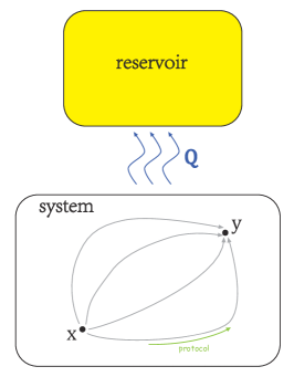
Figure 1: A system coupled with a heat reservoir evolves from state $x$ to state $y$ under a driving protocol. The system may travel through different trajectories in different attempts. Each trajectroy is endowed with a specific amount of heat released to the reservoir. $Q$ is the average amount of heat release over all trajectories from $x$ to $y$.

II Preliminaries

II.1 Algorithmic information theory

We briefly sketch the notations and results of algorithmic information theory(AIT) that are used in this paper. For a more complete introduction, readers can refer to liKolmogorovComplexityIts1990 , caludeInformationRandomnessAlgorithmic2002 and grunwaldShannonInformationKolmogorov2004 .

AIT is a theory on the "complexity" of objects (sequences, numbers, functions, etc.). By the term "complexity" of an object $x$, or $K(x)$ as is the usual notation, we mean the minimal resource required to "describe" $x$, which is often pinned down as (the length of) the shortest program $p$, when set as input for a (prefix-free) universal Turing machine $U$, generates $x$ as the output, that is:

$$K(x)\equiv\min\{l(p):U(p)=x\}.$$ (4)

As can be seen from above, $K(x)$ is dependent on the artificially chosen universal Turing machine $U$. However, this subjectivity can be saved by noticing that there exists an interpreter program $int(U,U^{\prime})$ between any two universal Turing machines $U$ and $U^{\prime}$, thus any program on $U^{\prime}$ can be run on $U$ by adding $int(U,U^{\prime})$ before the program. To be specific:

$$K_{U}(x)-K_{U^{\prime}}(x)\leq l(int(U,U^{\prime})),$$ (5)

and vice versa, so that

$$K_{U}(x)\overset{+}{=}K_{U^{\prime}}(x),$$ (6)

and there’s nothing lost in writing $K(x)$ instead of $K_{U}(x)$.

The Kolmogorov relative complexity $K(x|y)$ is similarly defined as (the length of) the shortest program $p$, when set as input for a (prefix-free) universal Turing machine $U$ coupled with a parameter tape writing $y$, which can be checked any time during the computation, generates $x$ as the output. To be specific:

$$K(x|y)\equiv\min\{l(p):U(p,y)=x\}.$$ (7)

The following statements of Kolmogorov complexity hold:

1. For every $x$, $y$ and $z$,

   $$K(x|z)\overset{+}{\leq}K(x,y|z)\overset{+}{\leq}K(x|y,z)+K(y|z).$$ (8)

2. Given a set $A$ with $|A|$ elements, for most $x\in A$, $K(x|A)\overset{+}{=}\log|A|$.

3. For every (computable) probability measure $P(x)$ (that is, $\sum_{x}p(x)=1$), $S_{sh}(P)\overset{+}{=}\sum_{x}P(x)K(x|P)$, where $S_{sh}(P)$ is the Shannon entropy of $P$.

4. For every (computable) relative probability semimeasure $P(x|y)$ (that is, $\sum_{x}P(x|y)\leq 1$ for every $y$), the coding theorem implies the inequality that

   $$K(x|y,P)\overset{+}{\leq}\log\frac{1}{P(x|y)}.$$ (9)

II.2 Stochastic thermodynamics

Stochastic thermodynamics is an emergent field that uses stochastic equations to study mesoscopic, nonequilibrium systems. Here we summary the notations and definitions used in this paper. More succinct introductions can be found in seifertStochasticThermodynamicsPrinciples2018 and shiraishiIntroductionStochasticThermodynamics2023 .

We consider a system with state space $\mathcal{X}$ coupled to a heat reservoir at reverse temperature $\beta$. There may be manipulations and/or drivings acting on the system. We assume the system undergoes a time-inhomogeneous Markov chain, and the jump rate from state $x$ to state $x^{\prime}$ at time $t$ is $k_{x^{\prime}x}(\lambda(t))$, where $\lambda(t)$ is the manipulation protocol acting on the system. As time passes from $t_{0}$ to $t_{n+1}$, the system may experience $n$ times of jumps from $x_{i}$ to $x_{i+1}$ at time $t_{i}(i=1,2,\cdots,n)$ and travel a trajectory $x(t)$:

$$x(t)=x_{i}\quad\mbox{for}\quad t_{i}\leq t\leq t_{i+1}.$$ (10)

Since the stochasticity of the system comes from its coupling with the heat reservoir, every time a jump occurs, there is heat released from the system to the reservoir. As is customary shiraishiIntroductionStochasticThermodynamics2023 , the heat released to the reservoir during a jump from $x$ to $x^{\prime}$ is assigned to be:

$$q_{x^{\prime}x}\equiv\log\frac{k_{x^{\prime}x}}{k_{xx^{\prime}}},$$ (11)

and the total heat released during a trajectory $x(t)$ is:

$$q(\bm{x})=\sum_{i=1}^{n}\log\frac{k_{x_{i}x_{i-1}}(t_{i})}{k_{x_{i-1}x_{i}}(t_{i})},$$ (12)

On the other hand, the probability density $P_{\bm{x}}(\bm{\lambda})$ for a trajectory $\bm{x}$ to occur with the forward protocol $\bm{\lambda}$ can be expressed as:

$$P_{\bm{x}}(\bm{\lambda})=p_{x_{0}}(t_{0})P_{\bm{x}|x_{0}}(\bm{\lambda}),$$ (13)

where $p_{x_{0}}(t_{0})$ is the probability of the system being in state $x_{0}$ at the beginning of the trajectory, and $P_{\bm{x}|x_{0}}(\bm{\lambda})$ is the relative probability density, which is given by:

$$P_{\bm{x}|x_{0}}(\bm{\lambda})=\prod_{i=1}^{n}k_{x_{i}x_{i-1}}(t_{i})2^{-\sum_{i=1}^{n}\int_{t_{i-1}}^{t_{i}}e_{x_{i-1}}(t)\differential t},$$ (14)

where $e_{x}\equiv\sum_{x^{\prime}\neq x}k_{x^{\prime}x}$ is the escape rate of state $x$.

We now consider the time-reverse process, or backward process, where both the trajectory and the protocol evolves in reverse order in time. The concept of backward process is critical in the derivation of various fluctuation theorems. We define $\tilde{t}\equiv t_{n+1}-(t-t_{0})$, $\tilde{x}(t)\equiv x(\tilde{t})$, $\tilde{\lambda}(t)\equiv\lambda(\tilde{t})$, and refer to $P_{\tilde{\bm{x}}|x_{n}}(\tilde{\bm{\lambda}})$ as the relative probability density of the backward trajectory.

Surprisingly, the ratio of $P_{\bm{x}|x_{0}}(\bm{\lambda})$ with $P_{\tilde{\bm{x}}|x_{n}}(\tilde{\bm{\lambda}})$ can be represented by the heat $q(\bm{x})$ released during the forward process $\bm{x}$ as in equation (12):

$$\frac{P_{\bm{x}|x_{0}}(\bm{\lambda})}{P_{\tilde{\bm{x}}|x_{n}}(\tilde{\bm{\lambda}})}=2^{q(\bm{x})}.$$ (15)

The above equation is the so-called detailed fluctuation theorem(DFT).

III Derivation of the bound

In this section, we shall derive the generalized Zurek’s bound, with the assumption that the system satisfies DFT.

First, let’s rewrite inequality (3) which we are going to prove:

$$K(x|y,\mathcal{P})\overset{+}{\leq}\log\frac{1}{P(y|x)}+Q(x\to y),$$ (16)

where $P(y|x)$ and $Q(x\to y)$ can be further expressed as:

$$P(y|x)=\sum_{\bm{x}:x_{f}=y}P_{\bm{x}|x}(\bm{\lambda}),$$ (17)

$$Q(x\to y)=\frac{1}{P(y|x)}\sum_{\bm{x}:x_{f}=y}P_{\bm{x}|x}(\bm{\lambda})q(\bm{x}),$$ (18)

where $x_{f}$ is the final state of the trajectory $\bm{x}$.

Since $P(\cdot|\cdot)$ and $Q(\cdot\to\cdot)$ can be computed from $\mathcal{P}$, to prove inequality (16), we only have to prove that the right-hand-side can be written as a negative logarithm of a semimeasure of $x$ given $y$ (the coding theorem), that is:

$$\sum_{x}2^{-(\log\frac{1}{P(y|x)}+Q(x\to y))}=\sum_{x}P(y|x)2^{-Q(x\to y)}\\ \leq\sum_{x}P(y|x)\frac{1}{P(y|x)}\sum_{\bm{x}:x_{f}=y}P_{\bm{x}|x}(\bm{\lambda})2^{-q(\bm{x})}\\ =\sum_{x}\sum_{\bm{x}:x_{f}=y}P_{\bm{x}|x}(\bm{\lambda})2^{-q(\bm{x})}=\sum_{x}\sum_{\bm{x}:x_{f}=y}P_{\bm{x}|x}(\bm{\lambda})\frac{P_{\tilde{\bm{x}}|y}(\tilde{\bm{\lambda}})}{P_{\bm{x}|x}(\bm{\lambda})}\\ =\sum_{x}\sum_{\tilde{\bm{x}}:\tilde{x_{f}}=x}P_{\tilde{\bm{x}}|y}(\tilde{\bm{\lambda}})=1,$$ (19)

where the first inequality comes from equation (18) and Jensen’s inequality and the third equality comes from the assumption of detailed fluctuation (15). Thus inequality (16) is proved.

Considering the inequality $K(x|y,\mathcal{P})\overset{+}{\leq}K(x|y)-K(\mathcal{P})$ as deduced from (8), we can write a weaker bound as:

$$Q(x\to y)+\log\frac{1}{P(y|x)}+K(\mathcal{P})\overset{+}{\geq}K(x|y).$$ (20)

As noted by KolchinskykolchinskyGeneralizedZurekBound2023 , the above inequality tells a trade-off between heat, noise and protocol complexity that has to be paid for the erased information in a computation from $x$ to $y$.

IV Applications

In this section, we discuss two applications of the generalized Zurek’s bound we just proved.

IV.1 Cost of erasure of an input sequence

Imagine $x$ is a binary sequence of length $n$ ($n$ may be large) and we want to set all the digits of $x$ to zero (to erase the sequence). If $x$ is a very random sequence, then $K(x|\mathcal{P})\approx n$. Since $K(0^{n}|\mathcal{P})\approx\log n\ll n$, the minimal heat release we have to pay for the erasure is approximately $n-\log\frac{1}{P(0^{n}|x)}$, so that if we hope to perform the erasure in a relatively high success rate, we have to pay for a cost proportional to the length of the sequence to be erased, which is consistent with the prediction given by Landauer’s principle.

However, if $x$ consists some kind of internal regularity, even if are unaware of that regularity and keep $\mathcal{P}$ unchanged, $K(x|\mathcal{P})$ can still be much smaller and less heat may be released in the erasure. For example, if all the bits on odd positions in $x$ are $1$, that is, $x$ is of the form $x_{0}1x_{2}1\cdots x_{n-2}1$, then $K(x|\mathcal{P})\approx n/2$, so that the minimal heat release to perform an erasure is reduced to a half in virtue of this regularity, which is a result cannot be concluded form Landauer’s principle.

IV.2 Condition for heat functions of nondeterministic Turing machines

In this part, we generalize previous results on the thermodynamic properties of Turing machineskolchinskyThermodynamicCostsTuring2020 to nondeterministic Turing machines.

A physical Turing machine is a protocol $\mathcal{P}$ that mimics the input-output relation $P:\mathcal{X}\to\mathcal{X}$ of a mathematical Turing machine. $\mathcal{P}$ is called a realization of $P$. A Turing machine is called (non)deterministic if $P$ is (non)deterministic.

Here (as in kolchinskyThermodynamicCostsTuring2020 ), we consider only the thermodynamic properties of physical Turing machines. Suppose a physical Turing machine $\mathcal{P}$ is coupled with a heat reservoir. When $\mathcal{P}$ is given an input $x$, an average amount of heat $Q(x)$ is released to the reservoir, that is:

$$Q(x)\equiv\sum_{y}P(y|x)Q(x\to y).$$ (21)

$Q(x)$ is called the heat function of $\mathcal{P}$.

It is proved in kolchinskyThermodynamicCostsTuring2020 that, when $P$ is deterministic, the heat function $Q(x)$ is realizable iff for every $y\in\mathcal{X}$, there is:

$$\sum_{x:P(x)=y}2^{-Q(x)}\leq 1.$$ (22)

Considering the form of the sum after the first equality in formula (19), we can easily generalize inequality (22) to any nondeterministic function $P$, and the heat function $Q(x\to y)$ is realizable iff for every $y\in\mathcal{X}$, there is:

$$\sum_{x}P(y|x)2^{-Q(x\to y)}\leq 1.$$ (23)

A dominating realization of $P$ is a realization $\mathcal{P}_{dom}$ whose heat function $Q_{dom}(x)$ is less than the heat function $Q(x)$ of any other realization of $P$ up to a constant additive term which may depend on $Q(\cdot)$. It is shown in kolchinskyThermodynamicCostsTuring2020 that for any realization of any deterministic $P$, the heat function $Q(x)$ obeys:

$$Q(x)\overset{+}{\geq}K(x|P(x))-K(Q,P).$$ (24)

Thus we can assign $Q_{dom}(x)=K(x|P(x))$ as the dominating heat function of $P$.

We can easily generalize inequality (24) to any nondeterministic function $P$, since inequality (24) is actually a deterministic restriction of the generalized Zurek’s bound (3). After rearrangement and note that $\mathcal{P}=(P,Q)$, we have:

$$Q(x\to y)\overset{+}{\geq}K(x|y,Q,P)-\log\frac{1}{P(y|x)}\\ \overset{+}{\geq}K(x|y)-\log\frac{1}{P(y|x)}-K(Q,P),$$ (25)

and the dominating heat function can be assigned as $Q_{dom}(x\to y)=K(x|y)-\log\frac{1}{P(y|x)}.$

V Future work

In this paper, we have studied the applications of Kolmogorov complexity in stochastic thermodynamics, especially the relationship between Kolmogorov complexity and fluctuation theorems. In Appendix B we will introduce an algorithmic definition of stochastic entropy that satisfies the integral fluctuation theorem.

So far, there are still many interesting problems at the intersection of AIT and thermodynamics but cannot be solved in our paradigm. For example, consider a process that realizes a computation of a very hard problem $f$ (such as 3SAT problem) but not erase the input, that is: $P(x)=(x,f(x))$ for a relatively high success rate. Since $f$ is very hard to compute), it is reasonable that this process should cost a lot(time, energy, etc.), but according to bound (3), $K(x,f(x)|x)\approx 0$ so no lower bound of the cost of this process can be acquired.

To solve the above problem, it may be helpful to consider resource-bounded Kolmogorov complexity, or to restrict our consideration to protocols that can be constructed from a limited set of subprograms (such as in wolpertStochasticThermodynamicsComputation2019 and wolpertThermodynamicsComputingCircuits2020 ). It would yield insightful results by applying the concepts and techniques of the well-established domain of computational complexity theory into the emergent field of stochastic thermodynamics.

APPENDIX A THE CONSTANT TERM IN THE GENERALIZED ZUREK’S BOUND

Many (in)equalities in this paper feature a constant additive term. In this appendix, we show that the constant term can actually be omitted in practical applications.

All the constant terms essentially come from the artificial choice of a universal Turing machine, as the length of the interpreter in inequality (5). To be more specific, it is reasonable to assume that $l(int(U,U^{\prime}))\approx K_{U}(U^{\prime})$. We also suppose that $U^{\prime}$ is a universal Turing machine with $s$ states and $a$ symbols. Since there are in total $2^{s^{2}a^{2}}$ (nondeterministic) Turing machines with $s$ states and $a$ symbols, we may further assume $K_{U}(U^{\prime})\approx\log(2^{s^{2}a^{2}})=s^{2}a^{2}$. According to woodsComplexitySmallUniversal2009 , the smallest universal Turing machines can make $s^{2}a^{2}\approx 10^{2}$bits. Convert bits to Joule per Kelvin:

$$10^{2}\operatorname{bits}=10^{-21}\operatorname{JK^{-1}},$$

which is a negligible amount in comparison to practically interesting thermodynamic quantities.

APPENDIX B AN ALGORITHMIC DEFINITION OF STOCHASTIC ENTROPY

In this appendix, we introduce an algorithmic definition of stochastic entropy following gacsBoltzmannEntropyRandomness1994 and ebtekarAlgorithmicSecondLaw2023 , and derive an integral fluctuation theorem (IFT) of it.

Consider a time-inhomogenuous Markovian system with (meso)state space $\mathcal{X}$. It is a common practice to assign a stochastic entropy (the total entropy of the composite system of the system and the reservoir) to every single state $x\in\mathcal{X}$ seifertStochasticThermodynamicsPrinciples2018 :

$$s_{sto}(x)\equiv-\log p_{x}(t)-f_{x}(t),$$ (26)

where $p_{x}(t)$ is the probability of the system being in state $x$ at time $t$, and $f_{x}(t)$ is the free energy of state $x$. Because $p_{x}(t)$ depends on the prepared state distribution $p_{x}(0)$, the stochastic entropy of the system depends not only on the state $x$ but also on the prepared state distribution at time $t=0$, which is not a favorable property since we prefer the entropy of the system to be a pure state function.

As in gacsBoltzmannEntropyRandomness1994 and ebtekarAlgorithmicSecondLaw2023 , we can define an entropy function of the system to depend only on $x$. To be concrete, we define the algorithmic entropy as:

$$s_{alg}(x)\equiv K(x|\mathcal{P})-f_{x}(t).$$ (27)

Since $p_{x}(t)$ can be computed from $\mathcal{P}$, the coding theorem implies that $K(x|\mathcal{P})\overset{+}{\leq}-\log p_{x}(t)$, so that $s_{alg}(x)\overset{+}{\leq}s_{sto}(x)$.

We justify the above definition by demonstrating that $s_{alg}(x)$ can restore to Boltzmann and Gibbs entropy in different senses. If $x$ is restricted in a set $A$ with $|A|$ elements, then $K(x|A)\approx\log|A|$ which is the Boltzmann entropy. For every probability distribution $P(x)$, $S_{sh}(P)\overset{+}{=}\sum_{x}P(x)K(x|P)$, which means that Gibbs entropy is the ensemble average of the algorithmic entropy for any ensemble.

What’s more, in the following we derive the integral fluctuation theorem for $s_{alg}(x)$, thus proving the second law of the algorithmic entropy. ebtekarAlgorithmicSecondLaw2023 has derived the integral fluctuation theorem for a single jump, and here we generalize the previous result to any trajectory.

The integral fluctuation theorem states that for every prepared state distribution $p_{x}(0)$, there is:

$$\langle 2^{-\Delta s_{alg}(\bm{x})}\rangle_{\bm{x}}\overset{\times}{\leq}1,$$ (28)

where $\Delta s_{alg}(\bm{x})$ is the algorithmic entropy production during the trajectory $\bm{x}$, and $\langle\cdot\rangle_{\bm{x}}$ means averaging over trajectories.

From definition (27), $\Delta s_{alg}(\bm{x})$ can be expressed as:

$$\Delta s_{alg}(\bm{x})=q(\bm{x})+K(x_{f}|\mathcal{P})-K(x_{0}|\mathcal{P})$$ (29)

Thus we have:

$$\langle 2^{-\Delta s_{alg}(\bm{x})}\rangle_{\bm{x}}=\sum_{\bm{x}}P_{\bm{x}}(\bm{\lambda})2^{-q(\bm{x})-K(x_{f}|\mathcal{P})+K(x_{0}|\mathcal{P})}\\ =\sum_{\bm{x}}p_{x_{0}}(0)P_{\bm{x}|x_{0}}(\bm{\lambda})\frac{P_{\tilde{\bm{x}}|x_{f}}(\tilde{\bm{\lambda}})}{P_{\bm{x}|x_{0}}(\bm{\lambda})}2^{-K(x_{f}|\mathcal{P})+K(x_{0}|\mathcal{P})}\\ =\sum_{\bm{x}}p_{x_{0}}(0)P_{\tilde{\bm{x}}|x_{f}}(\tilde{\bm{\lambda}})2^{-K(x_{f}|\mathcal{P})+K(x_{0}|\mathcal{P})}\\ \overset{\times}{\leq}\sum_{\bm{x}}p_{x_{0}}(0)P_{\tilde{\bm{x}}|x_{f}}(\tilde{\bm{\lambda}})2^{K(x_{0}|x_{f},\mathcal{P})}\\ \overset{\times}{\leq}\sum_{\bm{x}}p_{x_{0}}(0)P_{\tilde{\bm{x}}|x_{f}}(\tilde{\bm{\lambda}})\frac{1}{\tilde{P}(x_{0}|x_{f},\mathcal{P})}=1,$$ (30)

where the second equality comes from (15), the first inequality comes from (8), and the second inequality comes from the coding theorem.

As shown in Appendix A, the constant multiplicative factor in (28) is negligible, thus by Jensen’s inequality we arrive at the second law of the algorithmic entropy:

$$\Delta S_{alg}\equiv\langle\Delta s_{alg}\rangle_{\bm{x}}\geq 0.$$ (31)

References

- (1) C. H. Bennett, “Demons, engines and the second law,” Sci Am, vol. 257, no. 5, pp. 108–116, Nov. 1987.
- (2) ——, “The thermodynamics of computation—a review,” Int J Theor Phys, vol. 21, no. 12, pp. 905–940, Dec. 1982.
- (3) W. H. Zurek, “Algorithmic randomness and physical entropy,” Phys. Rev. A, vol. 40, no. 8, pp. 4731–4751, Oct. 1989.
- (4) A. Kolchinsky, “Generalized zurek’s bound on the cost of an individual classical or quantum computation,” Phys. Rev. E, vol. 108, no. 3, p. 034101, Sep. 2023.
- (5) K. Micadei, G. T. Landi, and E. Lutz, “Quantum fluctuation theorems beyond two-point measurements,” Phys. Rev. Lett., vol. 124, no. 9, p. 090602, Mar. 2020.
- (6) M. Li and P. M. Vitányi, “Kolmogorov complexity and its applications,” in Algorithms and Complexity. Elsevier, 1990, pp. 187–254.
- (7) C. Calude, Information and Randomness: An Algorithmic Perspective, 2nd ed., ser. Texts in Theoretical Computer Science. Berlin ; New York: Springer, 2002.
- (8) P. Grunwald and P. Vitanyi, “Shannon information and kolmogorov complexity,” Oct. 2004.
- (9) U. Seifert, “Stochastic thermodynamics: From principles to the cost of precision,” Physica A: Statistical Mechanics and its Applications, vol. 504, pp. 176–191, Aug. 2018.
- (10) N. Shiraishi, An Introduction to Stochastic Thermodynamics: From Basic to Advanced, ser. Fundamental Theories of Physics. Singapore: Springer Nature Singapore, 2023, vol. 212.
- (11) A. Kolchinsky and D. H. Wolpert, “Thermodynamic costs of turing machines,” Phys. Rev. Research, vol. 2, no. 3, p. 033312, Aug. 2020.
- (12) D. H. Wolpert, “Stochastic thermodynamics of computation,” J. Phys. A: Math. Theor., vol. 52, no. 19, p. 193001, May 2019.
- (13) D. H. Wolpert and A. Kolchinsky, “Thermodynamics of computing with circuits,” New J. Phys., vol. 22, no. 6, p. 063047, Jun. 2020.
- (14) D. Woods and T. Neary, “The complexity of small universal turing machines: A survey,” Theoretical Computer Science, vol. 410, no. 4-5, pp. 443–450, Feb. 2009.
- (15) P. Gacs, “The boltzmann entropy and randomness tests,” in Proceedings Workshop on Physics and Computation. PhysComp ’94. Dallas, TX, USA: IEEE Comput. Soc. Press, 1994, pp. 209–216.
- (16) A. Ebtekar, “The algorithmic second law of thermodynamics,” Sep. 2023.