Using Multiple Outcomes to Improve the Synthetic Control Method

Abstract

When there are multiple outcome series of interest, Synthetic Control analyses typically proceed by estimating separate weights for each outcome. In this paper, we instead propose estimating a common set of weights across outcomes, by balancing either a vector of all outcomes or an index or average of them. Under a low-rank factor model, we show that these approaches lead to lower bias bounds than separate weights, and that averaging leads to further gains when the number of outcomes grows. We illustrate this via simulation and in a re-analysis of the impact of the Flint water crisis on educational outcomes.

Key words: panel data, synthetic control method, linear factor model

JEL classification codes: C13, C21, C23.

1 Introduction

The synthetic control method (SCM) estimates a treated unit’s counterfactual untreated outcome via a weighted average of observed outcomes for untreated units, with weights chosen to match the treated unit’s pre-treatment outcomes as closely as possible (Abadie et al., 2010). In many applications, researchers are interested in multiple outcome series at once, such as both reading and math scores in educational applications (e.g., Trejo et al., 2021), or both low-wage employment and earnings when studying minimum wage changes (e.g., Jardim et al., 2022). Other recent empirical examples include Billmeier and Nannicini (2013); Kleven et al. (2013); Bohn et al. (2014); Pinotti (2015); Acemoglu et al. (2016); Dustmann et al. (2017); Cunningham and Shah (2018); Kasy and Lehner (2022). There is limited practical guidance for using SCM in this common setting, however, and researchers generally default to estimating separate weights for each outcome.

Like other single-outcome SCM analyses, this separate SCM approach can run into two main challenges. At one extreme, poor pre-treatment fit, which is more likely with longer series, can lead to bias (Ferman and Pinto, 2021; Ben-Michael et al., 2021). At the other extreme, perfect or near-perfect pre-treatment fit, which is more likely with shorter series, can lead to finding SCM weights that overfit to idiosyncratic errors — rather than finding weights that balance latent factors (Abadie et al., 2010).

In this paper, we show that estimating a single set of weights common to multiple outcome series can help address these challenges. We consider two approaches. First, following several recent empirical studies, we find a single set of concatenated weights: SCM weights that minimize the imbalance in the concatenated pre-treatment series for all outcomes. Second, we find a single set of average weights: SCM weights that minimize the imbalance in a linear combination of pre-treatment outcomes; as the leading case, we focus on imbalance in the average standardized pre-treatment outcome series.

Under the assumption that the $K$ different outcome series share a similar factor structure, we derive finite-sample bounds on the bias for these two approaches, as well as bounds when finding separate SCM weights for each outcome series. We show that both the concatenated and averaging approaches reduce the potential bias due to overfitting to noise by a factor of $\frac{1}{\sqrt{K}}$ relative to the analysis that considers each outcome separately. We also show that the averaging approach further reduces the potential bias due to poor pre-treatment fit by a factor of $\frac{1}{\sqrt{K}}$ relative to both the separate and concatenated approaches. In particular, averaging reduces the amount of the noise, which both improves pre-treatment fit and reduces bias due to overfitting to noise.

We inspect other facets of the distribution of the bias for each of the three approaches via a Monte Carlo study. We then use our results to conduct a re-analysis of Trejo et al. (2021), who study the impact of the Flint water crisis on student outcomes in Flint, Michigan.

Overall, for a wide variety of SCM analyses with multiple outcomes, we recommend averaging across outcomes, after appropriate standardization, as a reasonable default procedure that effectively leverages the multiple outcomes for bias reduction.

Related literature.

Despite the many empirical examples of SCM with multiple outcomes, there is relatively limited methodological guidance for this setting. Robbins et al. (2017) consider this problem in the context of SCM with high-dimensional, granular data and consider different aggregation approaches. Amjad et al. (2019) introduce the Multi-Dimensional Robust Synthetic Control (mRSC) method, which fits a linear regression using a de-noised matrix of all outcomes concatenated together.

The closest paper to ours is independent work from Tian et al. (2023), who explore a similar setting and also develop a bias bound. Their theoretical results, however, hinge on finding perfect pre-treatment fit for all outcome series simultaneously, which can be especially challenging to achieve with many outcomes. Moreover, the authors only consider weights based on concatenated outcomes. By contrast, our bias bounds are valid even with imperfect pre-treatment fit, and our analysis shows how averaging can reduce finite sample error relative to concatenated weights.

Finally, we build on an expansive literature on the Synthetic Control Method for single outcomes; see Abadie (2021) for a recent review. In particular, several recent papers propose modifications to SCM to mitigate bias both due to imperfect pre-treatment fit (e.g., Ferman and Pinto, 2021; Ben-Michael et al., 2021) and bias due to overfitting to noise (e.g., Kellogg et al., 2021). We complement these papers by highlighting how researchers can also incorporate multiple outcomes to mitigate both sources of bias.

Plan for paper.

Section 2 sets up the problem. Section 3 discusses the underlying identifying assumptions for SCM and the extension to multiple outcomes. Section 4 then explores how to leverage multiple outcomes for estimation, including a brief discussion of inference. Sections 5 and 6 present a simulation study and re-analysis of Trejo et al. (2021), respectively. Section 7 concludes. The appendix includes proofs, additional derivations, and further technical discussion.

2 Preliminaries

2.1 Setup and notation

We consider an aggregate panel data setting of $N$ units and $T$ time periods. For each unit $i=1,\dots,N$ and at each time period $t=1,\dots,T$, we observe $K$ outcomes $Y_{itk}$ where $k=1,\dots,K$. We denote the exposure to a binary treatment by $W_{i}\in\{0,1\}$. We restrict our attention to the case where a single unit receives treatment, and follow the convention that this is the first one, $W_{1}=1$. The remaining $N_{0}\equiv N-1$ units are possible controls, often referred to as “donor units.” To simplify notation, we limit to one post-treatment observation, $T=T_{0}+1$, though our results are easily extended to larger $T$.

We follow the potential outcomes framework (Neyman, 1990 [1923]) and denote the potential outcome under treatment $w$ with $Y_{itk}(w)$. Implicit in our notation is the assumption that there is no interference between units. Under this setup, we can write the observed outcomes as $Y_{itk}=(1-W_{i})Y_{itk}(0)+W_{i}\mathbbm{1}\{t\leq T_{0}\}Y_{itk}(0)+W_{i}\mathbbm{1}\{t>T_{0}\}Y_{itk}(1)$. The treatment effects of interest are the effects on the $K$ outcomes for the treated unit in the post-treatment period, $\tau_{k}=Y_{1Tk}(1)-Y_{1Tk}(0)$. We collect the treatment effects into a vector $\bm{\tau}=(\tau_{1},\ldots,\tau_{K})\in\mathbb{R}^{K}$. Since we directly observe $Y_{1Tk}(1)=Y_{1Tk}$ for the treated unit, we focus on imputing the missing counterfactual outcome under control, $Y_{1TK}(0)$.

To ensure that the multiple outcomes have similar variance, we standardize each outcome series using its pre-treatment standard deviation. The resulting average across standardized outcomes is therefore akin to a precision-weighted average, which, as we will show below, reduces noise and bias relative to classical SCM. To aid in interpretation, we also change the sign of each outcome to follow the convention that positive has the same semantic meaning for all outcomes (e.g., higher test scores are more desirable).

Throughout, we will focus on de-meaned or intercept-shifted weighting estimators (Doudchenko and Imbens, 2017; Ferman and Pinto, 2021). We denote $\bar{Y}_{i\cdot k}\equiv\frac{1}{T_{0}}\sum_{t=1}^{T_{0}}Y_{itk}$ as the pre-treatment average for the $k$^th outcome for unit $i$, and $\dot{Y}_{itk}=Y_{itk}-\bar{Y}_{i\cdot k}$ as the corresponding de-meaned outcome. We consider estimators of the form:

$$\widehat{Y}_{1Tk}(0)\equiv\bar{Y}_{1\cdot k}+\sum_{i=2}^{N}\gamma_{i}\dot{Y}_{iTk},$$ (1)

where $\gamma\in\mathbb{R}^{N-1}$ is a set of weights. Our paper centers on how to choose the weights $\gamma$.

2.2 Review: SCM with a single outcome series

Our setup encompasses the classic synthetic control method applied separately to each series (Abadie and Gardeazabal, 2003; Abadie et al., 2010, 2015), adapted to have an intercept, as in Doudchenko and Imbens (2017) and Ferman and Pinto (2021). This is a de-meaned weighting estimator with weights chosen to optimize the pre-treatment fit for a single de-meaned outcome $k$:

$$q_{k}^{sep}(\gamma) = \sqrt{\frac{1}{T_{0}}\sum_{t=1}^{T_{0}}\left(\dot{Y}_{1tk}-\sum_{W_{i}=0}\gamma_{i}\dot{Y}_{itk}\right)^{2}}$$

The weights that minimize this objective are the synthetic control weights:

$$\hat{\gamma}^{sep}_{k} = \underset{{\gamma\in\Delta^{N_{0}}}}{\text{argmin}\;\;}q_{k}^{sep}(\gamma)^{2}.$$

We refer to these as separate weights, because we use a distinct set of weights to separately estimate the effect for each outcome. Typically, the weights $\gamma$ are constrained to the simplex $\Delta^{N_{0}}=\{\gamma\in\mathbb{R}^{N_{0}}\mid\gamma_{i}\geq 0,\sum_{i=2}^{N}\gamma_{i}=1\}$ as above. This ensures that the weights will be sparse and non-negative. However, other constraints are possible, allowing for negative but bounded weights. If there are multiple constrained minimizers, we could further add a regularization term to the objective; see e.g., Doudchenko and Imbens (2017).

The quality of the de-meaned SCM estimator is determined by whether $\widehat{Y}_{1Tk}(0)$ is a good estimate for $Y_{1Tk}(0)$. A familiar condition for this to be the case is that the SCM weights achieve a low (root mean squared) placebo treatment effect, i.e., $q_{k}^{sep}(\hat{\gamma}^{sep}_{k})$ is close to zero. Under some restrictions on the idiosyncratic errors and for a single treated unit and single outcome, Abadie et al. (2010) show that if $q_{k}^{sep}(\hat{\gamma}_{k}^{sep})$ = 0 then the bias in the (non-demeaned) SCM estimator will tend to zero as $T_{0}\rightarrow\infty$. In shorter panels, however, the SCM estimator can be subject to bias from overfitting to idiosyncratic errors even if the fit is excellent. The goal of our paper is to understand how to leverage multiple outcomes when constructing the synthetic control to reduce bias from this and other sources.

3 Leveraging Multiple Outcomes for SCM: Identification

In this section we outline the assumptions on the data generating process that will allow us to share information across multiple outcomes. We describe necessary and sufficient conditions for there to exist a single set of weights that achieves zero bias across all outcomes simultaneously, and give intuition and examples in terms of linear factor models.

Throughout, we make the following structural assumption on the potential outcomes under control, similar to Athey et al. (2021).

Assumption 1.

The outcome under control is generated as

$$Y_{itk}(0)=\alpha_{ik}+\beta_{tk}+L_{itk}+\varepsilon_{itk}$$

where the deterministic model component includes unit and time fixed effects $\alpha_{ik}$ and $\beta_{tk}$, with $\sum_{t=1}^{T}\beta_{tk}=0$ for all $k$. After incorporating the additive two-way fixed effects, the model component retains a term $L_{itk}$ with $\sum_{i=1}^{N}L_{itk}=0$ for all $t,k$ and $\sum_{t=1}^{T}L_{itk}=0$ for all $i,k$. The idiosyncratic errors $\varepsilon_{itk}$ are mean zero, independent of the treatment status $W_{it}$, and independent across units and outcomes.

This setup allows the model component to include $\alpha_{ik}$, a unit fixed effect specific to outcome $k$. We explicitly account for the presence of these fixed effects by de-meaning across pre-treatment periods within each unit’s outcome series.

3.1 Existence of common weights shared across outcomes

To begin, we first characterize the bias of a de-meaned weighting estimator under Assumption 1. For a set of weights $\gamma$ that is independent of the idiosyncratic errors in period $T$, $\widehat{Y}_{1Tk}(0)$ has bias:

$$\mathbb{E}_{\varepsilon_{T}}\left[Y_{1Tk}(0)-\widehat{Y}_{1Tk}(0)\right]=\beta_{Tk}\left(1-\sum_{i=2}^{N}\gamma_{i}\right)+L_{1Tk}-\sum_{i=2}^{N}\gamma_{i}L_{iTk},$$ (2)

where $Y_{1Tk}(0)$ is the $k$^th control potential outcome for the treated unit at time $T$. Here the expectation is taken over the idiosyncratic errors in period $T$.

From this we see that weights $\gamma$ will lead to an unbiased estimator for time $t$ and outcome $k$ if (i) the weights sum to one and (ii) the weighted average of the latent $L_{itk}$ for the donor units equals $L_{1tk}$ for the treated unit. Weights that satisfy these conditions for all time period/outcome pairs would yield an unbiased estimator for every $Y_{1tk}(0)$ simultaneously. We refer to such weights as oracle weights $\gamma^{\ast}$, since they remove the bias due to the presence of the unobserved model components $L_{itk}$.

Definition 1 (Oracle Weights).

The oracle weights $\gamma^{\ast}$ solve the following system of $(TK)+1$ equations

$$\left(\begin{array}[]{cc}L&\mathbf{1}_{N}\end{array}\right)^{\prime}\left(\begin{array}[]{c}-1\\ \gamma^{\ast}\end{array}\right)=\mathbf{0}_{TK},$$ (3)

where the first row of $L\in\mathbb{R}^{N\times(TK)}$ contains $L_{itk}$ for the treated unit and the remaining rows correspond to control units.

We show in Section 4 that if such oracle weights exist, we can pool information across outcomes by finding a single set of synthetic control weights that are common to all $K$ outcomes. Such weights will exist if and only if the underlying matrix of model components $L$ is low rank. We formalize this in the following assumption and proposition.

Assumption 2a (Low-rank $L$).

The $N\times(TK)$ matrix of model components has reduced rank, that is,

$$rank(L)<N-1.$$

Proposition 1 (Low-rank is sufficient and necessary).

The unconstrained oracle weights $\gamma^{\ast}$ exist iff Assumption 2a holds.

3.2 Interpretation for linear factor models

Proposition 1 shows that determining whether oracle weights exist is equivalent to determining whether the model component matrix $L$ is low rank. We now discuss when this assumption is plausible and how it relates to the more familiar low rank assumptions used in the panel data literature.

To further interpret these restrictions, it is useful to express the model components $L$ in terms of a linear factor model. Under Assumption 2a, for $r=rank(L)$ the deterministic model component can be written as a linear factor model,

$$L_{itk}=\bm{\phi}_{i}\cdot\bm{\mu}_{tk},$$ (4)

where $\bm{\mu}_{tk}\in\mathbb{R}^{r}$ are latent time- and outcome-specific factors and each unit has a vector of time- and outcome-invariant factor loadings $\bm{\phi}_{i}\in\mathbb{R}^{r}$. Proposition 1 guarantees that oracle weights exist and solve

$$\bm{\phi}_{1}=\Phi_{0}^{\operatorname{tr}}\gamma^{\ast}$$

where the matrix $\Phi_{0}\in\mathbb{R}^{(N-1)\times r}$ collects the factor loadings $\phi_{i}$ for control unit $i=2,\dots,N.$

To interpret this factor structure, note that a special case that satisfies Assumption 2a is where the model component $L_{itk}$ can be decomposed into a common component that is shared across outcomes and an idiosyncratic, outcome-specific component:

$$L_{itk}=\sum_{f=1}^{r_{0}}\phi_{cf}\mu_{tkf}+\sum_{f=r_{0}+1}^{r_{k}}\phi_{kf}\mu_{ktf},$$ (5)

where all $\phi_{cf}$ and $\phi_{kf}$ are orthogonal to each other. Let $r_{0}$ denote the dimension of the factor loadings that are shared across the outcomes. Then we can calculate $rank(L)=r_{0}+\sum_{k=1}^{K}(r_{k}-r_{0})$, where there are $r_{0}$ common factor loadings and $(r_{k}-r_{0})$ idiosyncratic factor loadings for outcome $k$. The factor loadings can be seen as latent feature vectors associated with each unit, which may vary with the outcomes of interest. The low-rank Assumption 2a then states that $r_{0}+\sum_{k=1}^{K}(r_{k}-r_{0})<N-1$. This can happen when either the number of outcomes $K$ is relatively small or $r_{0}$ is large compared to $r_{k}$ so that there is a high degree of shared information across outcomes.

Example 1 (Repeated measurements of the same outcome).

An extreme case is where $Y_{it1},\ldots Y_{itK}$ are $K$ repeated measurements of the same outcome. In this case $\mu_{tk}=\mu_{t}$ for $k=1,\dots,K$, there are no idiosyncratic terms, and the rank of $L$ is $r_{0}$.

Example 2 (Multiple test scores).

Even with different outcomes, in many empirical settings, such as standardized test scores, there are only a few factors that explain most of the variation across outcomes, so $\sum_{k=1}^{K}(r_{k}-r_{0})$ is small and the low-rank assumption is plausible. For example, across seven test scores collected by Duflo et al. (2011), “average verbal” and “average math” explain 72% of the total variation.

Even if oracle weights that balance model components across all $K$ outcomes exist, estimating weights can be challenging without further restrictions. For example, there may be infinitely many solutions to Equation (3). We therefore introduce the following regularity condition that a set of oracle weights with a bounded norm exists.

Assumption 2b.

Assume $rank(L)<N-1$ and assume there is a known $C$ such that some oracle weights exist in a set $\mathcal{C}$ where $\|x\|_{1}\leq C$ for all $x\in\mathcal{C}$. Denote $\gamma^{\ast}$ as a solution to Equation (3) in $\mathcal{C}$.

Below, we will estimate synthetic control weights that are constrained to be in $\mathcal{C}$; Assumption 2b ensures that this set contains at least some oracle weights, allowing us to compare the synthetic control and oracle weights. This assumption further ensures that these oracle weights are not too extreme, as measured by the sum of their absolute values. While we keep the constraint set $\mathcal{C}$ general in our formal development, in practice—and in our empirical analysis below—this constraint set is often taken to be the simplex $\mathcal{C}=\Delta^{N-1}$, where $C=1$. This adds the stronger assumption that there exist oracle weights that are non-negative, and so the model component for the treated unit $L_{1\cdot}\in\mathbb{R}^{TK}$ is contained in the convex hull of the model components for the donor units, $\text{conv}\{L_{2\cdot},\ldots,L_{N\cdot}\}$.

4 Leveraging Multiple Outcomes for SCM: Estimation

We now turn to estimation. When common oracle weights across outcomes exist, they can yield unbiased estimates across all $K$ outcomes simultaneously. In that case, we seek to estimate a single set of weights across all $K$ outcomes that is approximately unbiased. In this section we consider two ways to do so: (i) finding one set of weights that balances all standardized outcomes, and (ii) finding one set of weights that balances the average across the standardized outcomes. We then establish bias bounds for both methods and separate SCM. Our findings indicate that under some conditions, both methods reduce bias due to overfitting compared to separate SCM and the averaging approach further reduces bias due to poor pre-treatment fit.

4.1 Measures of imbalance

In principle, we would like to find oracle weights that can recover $L_{1Tk}$ from a weighted average of $L_{2Tk},\ldots,L_{NTk}$ for all $k$. Since the underlying model components are unobserved, however, we must instead use observed outcomes $Y$ to construct feasible balance measures. In Section 2.2 above, we reviewed that the outcome $k$-specific imbalance measure $q^{sep}_{k}(\gamma)$ is the relevant criterion for separate SCM for each outcome series in the classic synthetic control literature (Abadie and Gardeazabal, 2003; Abadie et al., 2010, 2015).

Motivated by the common factor structure, we now consider two alternative balance measures that use information from multiple outcome series. First, we consider the concatenated objective, which simply concatenates the different outcome series together. This is the pre-treatment fit achieved across all standardized outcomes and pre-treatment time periods simultaneously:

$$q^{cat}(\gamma)\equiv\sqrt{\frac{1}{T_{0}}\frac{1}{K}\sum_{k=1}^{K}\sum_{t=1}^{T_{0}}\left(\dot{Y}_{1tk}-\sum_{W_{i}=0}\gamma_{i}\dot{Y}_{itk}\right)^{2}},$$

with corresponding weights

$$\hat{\gamma}^{cat}\equiv\underset{\gamma\in\mathcal{C}}{\text{argmin}\;\;}q^{cat}(\gamma)^{2}.$$

We refer to the set of weights that minimize this objective as the concatenated weights.

An alternative choice is the averaged objective, the pre-treatment fit for the average of the standardized outcomes:

$$q^{avg}(\gamma)\equiv\sqrt{\frac{1}{T_{0}}\sum_{t=1}^{T_{0}}\left(\frac{1}{K}\sum_{k=1}^{K}\dot{Y}_{1tk}-\sum_{W_{i}=0}\gamma_{i}\dot{Y}_{itk}\right)^{2}},$$

with corresponding weights

$$\hat{\gamma}^{avg}\equiv\underset{\gamma\in\mathcal{C}}{\text{argmin}\;\;}q^{avg}(\gamma)^{2}.$$

We refer to the set of weights that minimize this objective as the average weights.

Note that, for any realization of the data, the pre-treatment fit will be better for the averaged objective than for the concatenated objective, $q^{avg}(\hat{\gamma}^{avg})\leq q^{cat}(\hat{\gamma}^{cat})$. This finite-sample improvement in the fit also translates to a smaller upper bound on the bias, as we discuss next.

4.2 Estimation error

We first decompose the estimation error into the error due to bias and the error due to noise, then further decompose and bound the bias in Section 4.3. For any estimated weights $\hat{\gamma}$, the estimation error is

$$\tau_{k}-\hat{\tau}_{k}(\hat{\gamma}) =\dot{Y}_{1Tk}(0)-\sum_{i=2}^{N}\hat{\gamma}_{i}\dot{Y}_{itk}$$

$$=\underbrace{L_{1Tk}-\sum_{i=2}^{N}\hat{\gamma}_{i}L_{iTk}}_{\text{bias = imbalance + overfitting}}\;\;+\;\;\underbrace{\dot{\varepsilon}_{1Tk}-\sum_{i=2}^{N}\hat{\gamma}_{i}\dot{\varepsilon}_{iTk}}_{\text{noise}}.$$

The second term in the decomposition is due to post-treatment idiosyncratic errors and is common across the different approaches for choosing weights. In Appendix B.3 we show that this term has mean zero and can be controlled if the weights are not extreme.

Our main focus will be the first term, the bias due to inadequately balancing model components. Specifically, we can decompose this into two terms using the linear factor model in (4):

$$L_{1Tk}-\sum_{W_{i}=0}\hat{\gamma}_{i}L_{iTk} =\sum_{t=1}^{T_{0}}\sum_{j=1}^{K}{\omega}_{tj}\left(\dot{Y}_{1tj}-\sum_{W_{i}=0}\hat{\gamma}_{i}\dot{Y}_{itj}\right)\ \ (R_{0})$$ (6)

$$-\sum_{t=1}^{T_{0}}\sum_{j=1}^{K}{\omega}_{tk}\left(\dot{\varepsilon}_{1tj}-\sum_{W_{i}=0}\hat{\gamma}_{i}\dot{\varepsilon}_{itj}\right)\ \ (R_{1})$$ (7)

where the time and outcome specific terms $\omega_{tj}$ are transformations of the factor values that depend on the specific estimator.

The first term, $R_{0}$, is bias due to imperfect pre-treatment fit in the pre-treatment outcomes, $\dot{Y}_{itj}$. The second term, $R_{1}$, is bias due to overfitting to noise, also known as the approximation error. This arises because the optimization problems minimize imbalance in observed pre-treatment outcomes — noisy realizations of latent factors — rather than minimizing imbalance in the latent factors themselves.

4.3 Main result: Bias bounds

4.3.1 Additional assumptions

To derive finite sample bias bounds, we place structure on the idiosyncratic errors, assuming they are independent across time and do not have heavy tails.

Assumption 3.

The idiosyncratic errors $\varepsilon_{itk}$ are sub-Gaussian random variables with scale parameter $\sigma$.

Note that this assumption encompasses the setting where the idiosyncratic errors have a larger variance for certain outcomes; in this case the common scale parameter $\sigma$ is the maximum of the outcome-specific scale parameters. In practice, however, we assume that the variances of idiosyncratic errors across outcomes are equal after standardization. As a result, the simple average is also the precision-weighted average.

Finally, we assume an adequate signal to noise ratio for each outcome separately, for all outcomes jointly, and for the average across outcomes. Previous literature introduces similar assumptions to avoid issues of weak identification (Abadie et al., 2010). This additional assumption precludes settings where averaging removes substantial variation in the latent model components over time. Consider, for example, a setting where the model components for different outcomes vary over time in exactly opposite directions. Here averaging would cancel out any signal from their latent model components, and, as a result, our theoretical guarantees for the average weights would no longer hold. However, we can generally rule out these edge cases by economic reasoning or visual inspection of the co-movement across outcomes.

Assumption 4.

Denote $\bm{\mu}_{tk}\in\mathbb{R}^{r}$ as the time-outcome factors from Equation (4) and assume that they are bounded above by $M$. Furthermore, denoting $\sigma_{\text{min}}(A)$ as the smallest singular value of a matrix $A$, assume that (i) $\sigma_{min}\left(\frac{1}{T_{0}}\sum_{t}\mu_{tk}\mu_{tk}^{\prime}\right)\geq\underline{\xi}^{sep}>0$ for all outcomes $k=1,\dots,K$; (ii) $\sigma_{min}\left(\frac{1}{T_{0}K}\sum_{tk}\mu_{tk}\mu_{tk}^{\prime}\right)\geq\underline{\xi}^{cat}>0$; and (iii) $\sigma_{min}\left(\frac{1}{T_{0}}\sum_{t}\left(\bar{\mu}_{t}\right)\left(\bar{\mu}_{t}\right)^{\prime}\right)\geq\underline{\xi}^{avg}>0$ where $\bar{\mu}_{t}=\frac{1}{K}\sum_{k=1}^{K}\mu_{tk}$.

4.3.2 Bias bounds

With this setup, we now formally state the high-probability bounds on the bias terms in Equations (6) and (7) for the three weighting approaches. These bounds hold with high probability over the noise in all time periods and all outcomes, $\varepsilon_{itk}$. We can compare these high-probability for fixed $N$ as the number of time periods $T$ and/or the number of outcomes $K$ grow.

Theorem 1.

Suppose Assumptions 1, 2b,  3 and  4 hold. Recall that by construction, the estimated weights satisfy $\|\hat{\gamma}\|_{1}\leq C$ and Assumption 2b implies $\|\gamma^{\ast}\|_{1}\leq C$. Let $\tilde{\sigma}=(1+1/\sqrt{T_{0}})\sigma$. For any $\delta>0$, the absolute bias for estimating the treatment effect $\left|L_{1Tk}(0)-\sum_{W_{i}=0}\hat{\gamma}_{i}L_{iTk}\right|$ satisfies the bound

1. if analyzing $\hat{\gamma}_{k}^{sep}$,

   $$\leq\frac{r_{k}M^{2}}{\underline{\xi}^{sep}}\left(4(1+C)\sigma+2\delta+\frac{1}{\sqrt{T_{0}}}\left(2C\sqrt{\log 2N_{0}}+(1+C)\delta\right)\tilde{\sigma}\right),$$

   with probability at least $1-8\exp\left(-\frac{\delta^{2}}{2}\right)-4\exp\left(-\frac{T_{0}\delta^{2}}{2\sigma^{2}(1+C^{2})}\right)$.

2. if analyzing $\hat{\gamma}^{cat}$,

   $$\leq\frac{rM^{2}}{\underline{\xi}^{cat}}\left(4(1+C)\tilde{\sigma}+2\delta+\frac{1}{\sqrt{T_{0}K}}\left(2C\sqrt{\log 2N_{0}}+(1+C)\delta\right)\tilde{\sigma}\right),$$

   with probability at least $1-8\exp\left(-\frac{\delta^{2}}{2}\right)-4\exp\left(-\frac{T_{0}K\delta^{2}}{2\sigma^{2}(1+C^{2})}\right)$.

3. if analyzing $\hat{\gamma}^{avg}$,

   $$\leq\frac{rM^{2}}{\underline{\xi}^{avg}}\left(\frac{1}{\sqrt{K}}4(1+C)\sigma+2\delta+\frac{1}{\sqrt{T_{0}K}}\left(2C\sqrt{\log 2N_{0}}+(1+C)\delta\right)\tilde{\sigma}\right),$$

   with probability at least $1-8\exp\left(-\frac{\delta^{2}}{2}\right)-4\exp\left(-\frac{T_{0}K\delta^{2}}{2\sigma^{2}(1+C^{2})}\right).$

The proof for Theorem 1 relies on bounding the discrepancy in the objectives between estimated and oracle weights. In Lemma 4 in the Appendix, we also derive finite-sample error bounds for the oracle weights themselves and show a similar ordering for the bounds on average, concatenated, and separate objectives. Table 1 gives a high-level overview of these results and shows the leading terms in the bounds, removing terms that do not change with $K$ and $T_{0}$. We discuss implications of our results next.

	Bias due to imperfect fit	Bias due to overfitting
$\hat{\gamma}^{sep}$	$O(1)$	$O\left(\frac{1}{\sqrt{T_{0}}}\right)$
$\hat{\gamma}^{cat}$	$O(1)$	$O\left(\frac{1}{\sqrt{T_{0}K}}\right)$
$\hat{\gamma}^{avg}$	$O\left(\frac{1}{\sqrt{K}}\right)$	$O\left(\frac{1}{\sqrt{T_{0}K}}\right)$

Table 1: Leading terms in high probability bounds on the bias due to imperfect fit and overfitting in Theorem 1, with $N$ fixed.

4.4 Discussion: Bias decomposition

Our analysis differs from the existing literature in two key ways. First, the results for (non-de-meaned) synthetic controls with a single outcome from Abadie et al. (2010) are based on an upper bound on $R_{1}$ while assuming $R_{0}=0$. Instead we show explicit finite sample upper bounds for $R_{0}$ and generalize these bounds to incorporate multiple outcomes. Second, we quantify the impact of demeaning with a finite number of pre-treatment time periods $T_{0}$; this contributes to additional bias (often known as “Nickell bias” due to Nickell, 1981) but vanishes as $T_{0}$ grows large. These finite-sample bounds extend existing asymptotic results from Ferman and Pinto (2021).

For both the separate weights $\hat{\gamma}_{k}^{sep}$ and the concatenated weights $\hat{\gamma}^{cat}$, imperfect pre-treatment fit—on outcome $k$ alone for the separate weights, and on all outcomes for the concatenated weights—contributes to bias, regardless of the number of pre-treatment periods or outcomes. This result is consistent with Ferman and Pinto (2021) who show that as $T_{0}\rightarrow\infty$, the separate objective function $q_{k}^{sep}(\gamma)$ does not converge to the objective minimized by the oracle weights, and therefore remains biased. In contrast, the bias due to pre-treatment fit for the average weights will decrease with the number of outcomes $K$. This is because averaging across outcomes reduces the level of noise in the objective. With many outcomes, the average will be a good proxy for the underlying model components that themselves can be exactly balanced by the oracle weights. Averaging therefore allows us to get close to an oracle solution, with low bias due to pre-treatment fit. This result is also consistent with Ferman and Pinto (2021) since the variance of the noise decreases to zero as both $K$ and $T_{0}\to\infty$ grow. Note, however, that the bounds are scaled by the rank $r$ of the underlying model matrix when pooling information across outcomes; so if the outcomes share few common factors and have many idiosyncratic ones, there may be more error in the estimator relative to separately fitting the weights.

The second component of the bias is the contribution of overfitting to noise. Mirroring prior results (e.g., Abadie et al., 2010), we find that the threat of overfitting to noise with separate synthetic control weights will decrease as the number of pre-treatment periods $T_{0}$ increases — but remains unchanged as $K$ increases. In contrast, the bias from overfitting to noise for both the concatenated and the averaged weights will decrease as the product $T_{0}K$ increases, albeit for different reasons. For the concatenated weights, the extra outcomes essentially function as additional time periods. Each time period-outcome pair gives another noisy projection of the underlying latent factors, and finding a single good synthetic control for all of these together limits the threat of overfitting to any particular one. For averaged weights, averaging across outcomes directly reduces the noise of the objective, as we discuss above. The $T_{0}$ averaged outcomes will therefore have a standard deviation that is smaller by $\approx\frac{1}{\sqrt{K}}$ than the original outcome series, leading to less noise and less potential for overfitting.

Finally, for all three estimators the component due to overfitting to noise in Theorem 1 includes an additional term that scales like $O(1/T_{0})$ as $T_{0}$ increases, and so is not a leading term. This is an example of Nickell (1981) bias and arises due to de-meaning by the estimated, rather than true, unit fixed effects.

4.5 Inference

There is a large and growing literature on inference for the synthetic control method and variants. Here we adapt the conformal inference approach of Chernozhukov et al. (2021) to the setting of multiple outcomes. To do so, we focus on a sharp null hypothesis about the effects on the $K$ different outcomes simultaneously, $H_{0}:\bm{\tau}=\bm{\tau}_{0}$, with $\bm{\tau}\in\mathbb{R}^{K}$. For example, if $\bm{\tau}_{0}=\mathbb{0}_{K}$ we are interested in testing whether the treatment effect is zero for all outcomes.

The conformal inference approach proceeds as follows:

1. Enforce the null hypothesis by creating adjusted post-treatment outcomes for the treated unit $\tilde{Y}_{1Tk}=Y_{1Tk}-\tau_{0k}$.

2. Augment the original data set to include the post-treatment time period $T$, with the adjusted outcomes $\tilde{Y}_{1Tk}$; use the concatenated or averaged objective function to obtain weights $\hat{\gamma}(\bm{\tau}_{0})$

3. Compute the adjusted residual $\hat{u}_{tk}=Y_{1tk}-\sum_{W_{i}=0}\hat{\gamma}_{i}(\bm{\tau}_{0})Y_{itk}$ and $\hat{u}_{Tk}=\tilde{Y}_{1Tk}-\sum_{W_{i}=0}\hat{\gamma}_{i}(\bm{\tau}_{0})Y_{iTk}$ and form the test statistic:

   $$S_{q}(\hat{u}_{t})=\left(\frac{1}{\sqrt{K}}\sum_{k=1}^{K}|\hat{u}_{tk}|^{q}\right)^{1/q}$$ (8)

   where the choice of the norm $q$ maps to power against different alternatives. For instance, if the treatment has a large effect for only few outcomes, choosing $q=\infty$ yields high power. On the other hand, if the treatment effect has similar magnitude across all outcomes, then setting $q=1$ or $q=2$ yields good power. In practice, we set $q=1$.

4. Compute a $p$-value by assessing whether the test statistic associated with the post-treatment period “conforms” with the distribution of the test statistic associated with pre-treatment periods:

   $$\hat{p}(\bm{\tau}_{0})=\frac{1}{T}\sum_{t=1}^{T_{0}}\bm{1}\left\{S_{q}(\hat{u}_{T})\leq S_{q}(\hat{u}_{t})\right\}+\frac{1}{T}.$$ (9)

Chernozhukov et al. (2021) show that in an asymptotic setting with $T$ (and $N$) growing, this conformal inference procedure will be valid for estimation methods that are consistent. In particular, they show that the test (9) has approximately correct size; the difference between actual size and nominal size vanishes as $T_{0}\rightarrow\infty$. In Appendix A we discuss technical sufficient conditions for consistency, closely following Chernozhukov et al. (2019) and departing from the finite-sample analysis that is our main focus here.

To construct the confidence set for the treatment effect of different outcomes, we collect the values of $\bm{\tau}_{0}$ for which test (9) does not reject. We can then project the confidence set onto each outcome to form a conservative confidence interval.

Finally, an alternative approach is to focus on testing the average effect across the $K$ outcomes, $\frac{1}{K}\sum_{k=1}^{K}\tau_{k}$, with outcomes appropriately scaled so that positive and negative effects have the similar semantic meanings across outcomes. This setting returns to the scalar setting considered by Chernozhukov et al. (2021), where the estimates are based on the average weights $\hat{\gamma}^{avg}$, and so for inference on the average we can follow their procedure exactly.

5 Simulations

We now conduct a Monte Carlo study to further inspect the behavior of separate, concatenated, and average weights. In particular, Theorem 1 gives upper bounds on the bias term, describing the worst-case behavior of the estimators with high probability. Here we instead use simulation to inspect other features of the distribution of the bias, especially the average bias.

To focus on key ideas, we consider a simple model of the $k$^th outcome under control,

$$Y_{itk}(0)=\phi_{i}\mu_{t}+\varepsilon_{itk},$$

where $\phi_{i}$ is a scalar and $\varepsilon_{itk}\sim\mathcal{N}(0,1)$. Here multiple outcomes are in fact repeated measurements of the same underlying model component that consists of a single latent factor. We consider four settings for the number of pre-treatment time periods $T_{0}$ and outcomes $K$: (i) $T_{0}=10,K=4$; (ii) $T_{0}=10,K=10$; (iii) $T_{0}=40,K=4$; (iv) $T_{0}=40,K=10$.

We set the factor values $\mu_{t}$ to be evenly spaced over the interval $[0.5,1]$ for $t=1,\dots,T_{0}+1$, reflecting an upward time trend; the factor loadings $\phi_{i}$ are evenly spaced over the interval $[1,5]$ for $i=1,\dots,50$. Similar to Ferman (2021), we set the treated unit to be the unit with the second largest factor loading. This accomplishes two goals. First, it injects selection of the treated unit based on the factor loadings, so that a simple difference in means would be biased. Second, it guarantees the existence of oracle weights that solve $\phi_{1}-\sum_{W_{i}=0}\gamma_{i}^{\ast}\phi_{i}=0$. Note that since the time trend has a heterogenous effect across the units, the difference-in-differences estimator is also biased.

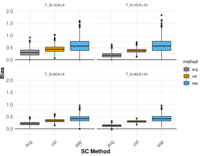
Figure 1: Box plots of bias using separate SCM, concatenated SCM, and averaged SCM over 1000 simulations.

Figure 1 compares the distribution of the bias for estimating the treatment effect on the first outcome under different weighting estimators:

$$\mathbb{E}\left[\hat{\tau}_{1}-\tau_{1}\right]=L_{1T1}-\sum_{W_{i}=0}\hat{\gamma}_{i}L_{iT1}.$$

Consistent with Theorem 1, Figure 1 illustrates that, relative to separate weights, the concatenated and average weights reduce bias in settings with multiple outcomes. We also see that, as expected, the average weights have smaller average bias than the concatenated weights.

To further inspect this, Appendix Figure E.1 contrasts the imbalance for each type of weight with the corresponding objective functions. First, the concatenated weights have slightly greater imbalance than the separate weights, highlighting the difficulty in achieving good pre-treatment fit on all outcomes simultaneously relative to good pre-treatment fit for a single outcome alone. However, the average bias for the concatenated weights is still smaller than for the separate weights, showing that the reduction in overfitting by concatenating more than outweighs the slight reduction in pre-treatment fit. Second, the average weights have much better pre-treatment fit than either alternative, with the fit improving as $K$ increases. As Figure 1 shows, this leads to further bias reduction, consistent with Theorem 1 and the intuition from Table 1.

6 Application: Flint Water Crisis Study

We now revisit the Trejo et al. (2021) study of the impact of the 2014 Flint water crisis on student outcomes. On April 25, 2014, Flint’s residents began receiving drinking water from the Flint River, where the water was both corrosive and improperly treated, causing lead from the pipes to leach into the tap water. Roughly 100,000 citizens of Flint were exposed to this polluted water for at least a year and a half — and likely much longer in some cases. Nearly a decade later, there are still widespread concerns about the impact of this crisis, especially on children, who are particularly susceptible to adverse effects from lead.

To assess this impact, Trejo et al. (2021) conduct several different analyses both across school districts and within Flint. We focus here on their cross-district SCM analysis, based on a district-level panel data set for Flint and 54 possible comparison districts in Michigan, viewing the April 2014 change in drinking water as the “treatment.” The authors focus on four key educational outcomes: math achievement, reading achievement, special needs status, and daily attendance; all are aggregated to the annual level from 2007 to 2019.

Trejo et al. (2021) argue that these four outcomes are indicative of (aggregate) student psycho-social outcomes at the district level, and, consistent with our results in Theorem 1, fit a common set of (de-meaned) SCM weights based on concatenating these outcome series. Here we return to that choice and also consider both separate and average SCM weights.

First, we assess whether the observed data are consistent with the low-rank factor model discussed in Section 3.1. To do so, we examine the $N\times T_{0}K$ matrix of (de-meaned and standardized) pre-treatment outcomes, where $N=54$, $T_{0}=8$, and $K=4$. In Appendix Figure E.2, we show that the top 10 singular values capture over 80% of the total variation, which is consistent with a low-rank model component and the existence of corresponding oracle weights.

Figure 2 shows the SCM gap plots — i.e. the differences between the observed outcomes for Flint and the counterfactual outcomes imputed by the synthetic control — for these three sets of weights. The separate SCM weights (long dashed line) achieve close to perfect fit in the pretreatment period, suggesting potential bias due to overfitting to noise, as we discuss in Section 4.4. By contrast, the concatenated and average SCM weights (dashed and solid, respectively) do not lead to near-perfect pre-treatment fit, though the fit is still reasonably good. Figure 3 shows the gap plot for the average of the (standardized) outcomes for both averaged and concatenated SCM; as we expect, we see that the concatenated weights achieve poorer fit for this index of outcomes than the average weights, substantially so at the beginning and end of the pre-treatment period.

Both averaged and concatenated weights estimate a deterioration of math test scores following the Flint water crisis, with little change in reading test scores and student attendance. Both sets of weights also find an increase in the proportion of students with special needs, though the magnitude is smaller for the averaged weights. Thus, the results largely replicate those in Trejo et al. (2021), although the estimates from average weights have slightly smaller magnitudes.

Finally, we use the conformal inference procedure discussed in Section 4.5 to assess uncertainty, with the caveat that the number of pre-treatment periods is only slightly larger than the number of post-treatment periods in this application. We first test the null hypothesis of no effect on any outcomes in each time period, using average SCM weights and i.i.d. permutations; this yields $p$-values of roughly $p\approx 0.1$ for each time period (for 2015-2019, these are 0.113, 0.098, 0.116, 0.098, and 0.108). We then test the joint null hypothesis of no effect on any outcomes in any time period via a conformal inference procedure using all post-treatment time periods; here we find strong evidence against the null of no effect whatsoever, with $p=0.007$.

In the appendix, we also consider analyzing the impact on special needs separately from the other three outcomes, consistent with the robustness checks in Trejo et al. (2021). In particular, the proportion of students with special needs may be less correlated with the other outcomes, and so may share fewer common factors, loosening the bound from Section 4.3. Appendix Figure E.3 shows that results are broadly similar when we restrict to math, reading, and attendance alone. The results are also broadly similar if we consider the proportion of students without special needs as an outcome in place of the original definition.

Figure 2: Point estimates for the effect of the Flint water crisis using SCM, concatenate SCM, and average SCM. Using i.i.d. permutations, the conformal $p$-values for the joint null hypothesis of no effect on any outcome for the 5 post treatment year 2015-2019 are: 0.113, 0.098, 0.116, 0.098, and 0.108. Note that the separate SCM estimates have essentially perfect pre-treatment fit for all four outcomes.

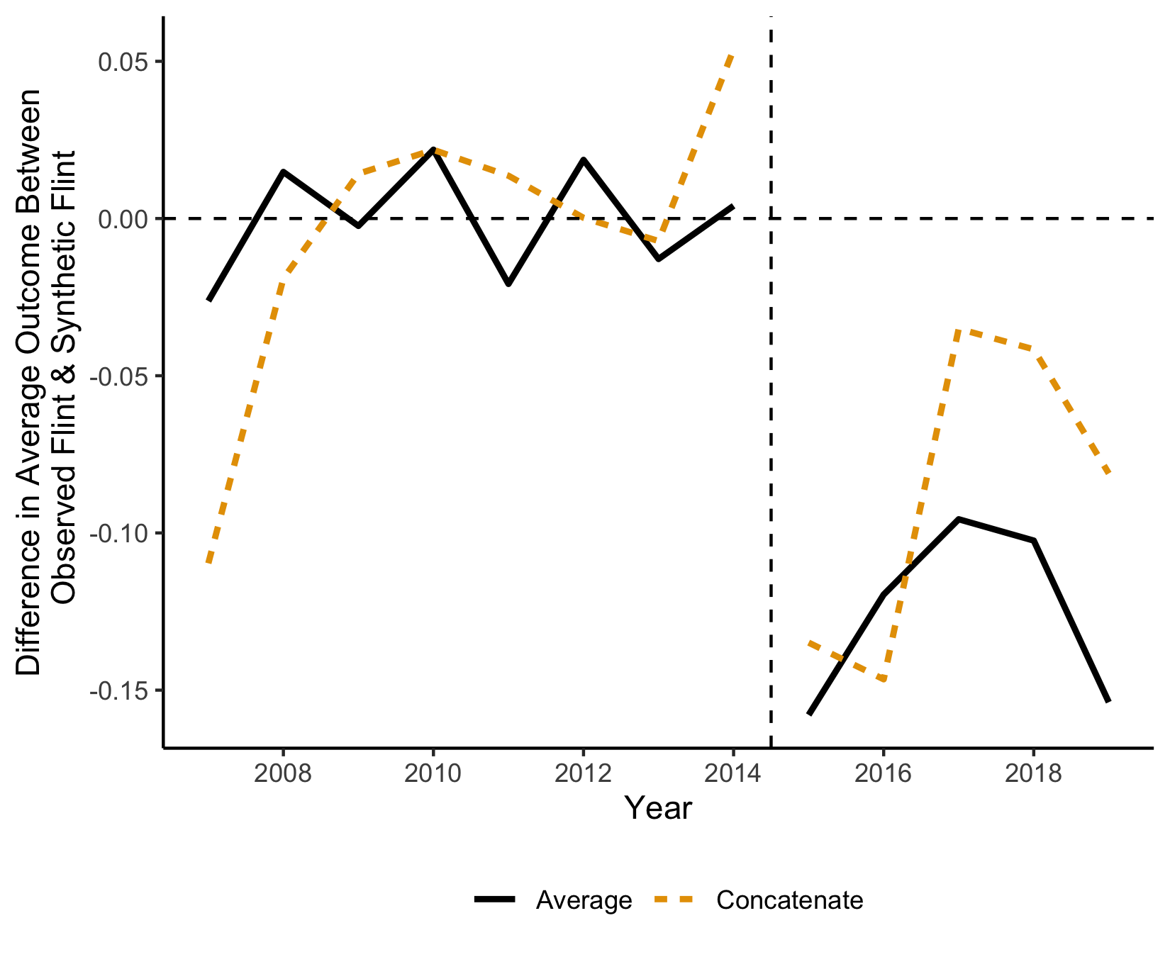
Figure 3: Fit for the average of the outcomes (standardized by the pre-treatment standard deviation of the series) using average SCM and concatenate SCM.

7 Conclusion

SCM is a popular approach for estimating policy impacts at the aggregate level, such as school district or state. This approach, however, can be susceptible to bias due to poor pre-treatment fit or to overfitting to idyosyncratic errors. By incorporating multiple outcome series into the SCM framework, this paper proposes approaches that address these challenges, provided that the multiple outcomes share a similar factor structure.

There are several directions for future work. The most immediate is to give guidance for SCM with multiple outcomes when the common factor structure might not in fact hold. One possibility is to consider weights that “partially pool” between separate SCM weights and common weights in the spirit of Ben-Michael et al. (2022), which could enable guarantees under mis-specification. More broadly, we could consider approaches that average or borrow strength across multiple model types, including from hierarchical Bayesian models (see, for example, Ben-Michael et al., 2023), from tensor completion following Agarwal et al. (2023) or from an instrumental variable approach following Shi et al. (2021) and Fry (2023).

Finally, leveraging multiple outcomes alone might not be enough to mitigate SCM bias. Following Ben-Michael et al. (2021) and Arkhangelsky et al. (2021), we could consider augmenting common SCM weights with either a common outcome model or separate models for each outcome series.

Appendix A Technical details regarding inference

In this section we provide additional technical details for the approximate validity of the conformal inference procedure proposed by Chernozhukov et al. (2021) with averaged weights. To do so, we will consider an asymptotic setting with both $N$ and $T$ growing, and make a variation of the structural Assumption 1 and Assumption 2b that constrained oracle weights exist.

Assumption 5.

The de-meaned potential outcome under control for the treated unit’s $k$th outcome at time $t$ is

$$\dot{Y}_{itk}(0)=\sum_{W_{i}=0}\gamma_{i}^{\ast}\dot{Y}_{itk}+u_{tk},$$

for some set of oracle weights $\gamma^{\ast}\in\mathcal{C}$, where for a given $k$ the noise terms $u_{1k},\ldots,u_{Tk}$ are stationary, strongly mixing, with a bounded sum of mixing coefficients bounded, and satisfy $\mathbb{E}[u_{tk}Y_{itk}]=0$ for all $W_{i}=0$.

As in the previous assumptions, Assumption 5 also assumes the existence of oracle weights $\gamma^{\ast}$ shared across all outcomes, though they are defined slightly differently. Directly applying Theorem 1 in Chernozhukov et al. (2021), the conformal inference procedure in Section 4.5 using a set of weights $\hat{\gamma}$, will be asymptotically valid if $\sum_{W_{i}=0}\hat{\gamma}_{i}\dot{Y}_{itk}$ is a consistent estimator for $\sum_{W_{i}=0}\gamma^{\ast}_{i}\dot{Y}_{itk}$, when we include the post-treatment period $T$ when estimating the weights.

Next, we list sufficient assumptions for this type of consistency using the average weights $\hat{\gamma}^{\text{avg}}$, consistency with the concatenated weights $\hat{\gamma}^{\text{cat}}$ can be established in an analogous matter. In these assumptions, we define $\bar{u}_{t}=\frac{1}{K}\sum_{k=1}^{K}u_{tk}$ and $\dot{\bar{Y}}_{it\cdot}=\frac{1}{K}\sum_{k=1}^{K}\dot{Y}_{itk}$.

Assumption 6.

1. There exist constants $c_{1},c_{2}>0$ such that $\mathbb{E}[\left(\dot{\bar{Y}}_{it\cdot}\bar{u}_{t}\right)^{2}\geq c_{1}$ and $\mathbb{E}[\left|\bar{Y}_{it\cdot}\bar{u}_{t}\right|^{3}]\leq c_{2}$ for any $i$ such that $W_{i}=0$ and $t=1,\ldots,T$.

2. For each $i$ such that $W_{i}=0$, the sequence $\{\dot{\bar{Y}}_{it\cdot}\bar{u}_{t}\}$ is $\beta$-mixing and the $\beta$-mixing coefficient satisfies $\beta(t)\leq a_{1}\exp\left(-a_{2}t^{\tau}\right)$, where $a_{1},a_{2},\tau>0$.

3. There exists a constant $c_{3}>0$ such that $\max_{i:W_{i}=0}\sum_{t=1}^{T}\dot{\bar{Y}}_{it\cdot}^{2}\bar{u}_{t}^{2}\leq c_{3}T$ with probability $1-o(1)$.

4. $\log N=o\left(T^{\frac{4\tau}{3\tau+4}}\right)$

5. There exists a sequence $\ell_{T}>0$ such that $\frac{\ell_{T}M[\log(\min\{T,N-1\})]^{\frac{1+\tau}{2\tau}}}{\sqrt{T}}\to 0$,

   $$\left(\sum_{W_{i}=0}\dot{Y}_{iTk}\delta_{i}\right)^{2}\leq\ell_{T}\frac{1}{T}\sum_{t=1}^{T}\left(\sum_{W_{i}=0}\dot{\bar{Y}}_{it\cdot}\delta_{i}\right)^{2},$$

   and

   $$\frac{1}{T}\sum_{t=1}^{T}\left(\dot{Y}_{itk}\delta_{i}\right)^{2}\leq\ell_{T}\frac{1}{T}\sum_{t=1}^{T}\left(\dot{\bar{Y}}_{it\cdot}\delta_{i}\right)^{2}$$

   for all $\gamma^{\ast}+\delta\in\mathcal{C}$, all $k=1,\ldots,K$ with probability $1-o(1)$.

Assumption 6 follows the technical assumptions in the proof of Lemma 1 in Chernozhukov et al. (2021) with two modifications. First, we place assumptions on the noise values averaged across outcomes, $\bar{u}_{1},\ldots\bar{u}_{T}$ rather than the outcome-specific noise values because we are working with the averaged estimator. Second, Assumption 6(v) modifies Assumption (6) in the proof of Lemma 1 in Chernozhukov et al. (2021) to link consistent prediction of the average of the de-meaned outcomes to consistent prediction for any individual outcome. This assumption is related to Assumption 2b. If there is a common factor structure across outcomes, then we have the link

$$\sum_{W_{i}=0}\dot{Y}_{itk}\delta_{i} =\mu_{tk}\cdot\sum_{W_{i}=0}\phi_{i}\delta_{i}+\sum_{W_{i}=0}\dot{\varepsilon}_{itk}\delta_{i}$$

$$=\mu_{Tk}\cdot\left(\sum_{t}\left(\bar{\mu}_{t}\right)\left(\bar{\mu}_{t}\right)^{\prime}\right)^{-1}\bar{\mu}_{t}\sum_{W_{i}=0}\dot{\bar{Y}}{it\cdot}\delta_{i}+\mu_{Tk}\cdot\left(\sum_{t}\left(\bar{\mu}_{t}\right)\left(\bar{\mu}_{t}\right)^{\prime}\right)^{-1}\bar{\mu}_{t}\sum_{W_{i}=0}\dot{\bar{\varepsilon}}_{it\cdot}\delta_{i}+\sum_{W_{i}=0}\dot{\varepsilon}_{itk}\delta_{i}.$$

So, if common oracle weights exist, Assumption 6(v) amounts to an assumption on the noise terms.

Under these assumptions, we have a direct analog to Lemma 1 in Chernozhukov et al. (2021) that is a direct consequence. We state it here for completeness.

Lemma 1.

Let $\hat{\gamma}^{\text{avg}}$ solve $\min_{\gamma\in\mathcal{C}}q^{\text{avg}}(\gamma)^{2}$, including the post treatment outcome $T$. Under Assumptions 5 and 6, $\hat{\gamma}^{\text{avg}}$ satisfies the consistency properties required for Theorem 1 in Chernozhukov et al. (2021), namely,

$$\frac{1}{T}\sum_{t=1}^{T}\left(\dot{Y}_{itk}\left(\hat{\gamma}_{i}-\gamma_{i}^{\ast}\right)\right)^{2}=o_{p}(1)$$

and

$$\dot{Y}_{iTk}\left(\hat{\gamma}_{i}-\gamma_{i}^{\ast}\right)=o_{p}(1).$$

Proof of Lemma 1.

First, we can directly apply the claim from the proof of Lemma 1 and Lemma H.8 in Chernozhukov et al. (2021) to state that there exists a constant $M>0$ such that

$$\frac{1}{T}\sum_{t=1}^{T}\left(\dot{\bar{Y}}_{it\cdot}(\hat{\gamma}_{i}^{\text{avg}}-\gamma^{\ast}_{i})\right)^{2}\leq\frac{M[\log(\min\{T,N-1\})]^{\frac{1+\tau}{2\tau}}}{\sqrt{T}}$$

with probability $1-o(1)$. Now from Assumption 6(v), $\frac{\ell_{T}M[\log(\min\{T,N-1\})]^{\frac{1+\tau}{2\tau}}}{\sqrt{T}}=o(1)$, which completes the proof. ∎

Appendix B Auxillary lemmas and proofs

B.1 Error bounds for the oracle imbalance

The bias due to imbalance in observed demeaned outcomes depends crucially on the measure of imbalance we choose to minimize. We upper bound the imbalance using the estimated weights with the imbalance when using oracle weights, which we refer to as oracle imbalance. For example, we argue the oracle imbalance for the objective function of the SCM satisfies a form of concentration inequality:

$$q^{sep}(\gamma^{\ast}) = \sqrt{\frac{1}{T_{0}}\sum_{t=1}^{T_{0}}\left(\dot{\varepsilon}_{1tj}-\sum_{W_{i}=0}\gamma^{\ast}_{i}\dot{\varepsilon}_{itj}\right)^{2}}$$

At first glance, the imbalance is the L2 norm of the vector of demeaned errors. The challenge is that the demeaned errors $\dot{\varepsilon}_{itj}$ are correlated over time due to demeaning.

We prove a general upper bound on the oracle imbalance in Lemma 2 that allow us to decompose the imbalance into the L2 norm of errors and the L2 norm of the average of errors. Lemma 3 presents the intermediate concentration inequality for the L2 norm of errors. Finally, building on Lemma 2 and 3, Lemma 4 inspects the numerical properties for the pre-treatment fits achievable by the oracle weights. Unless otherwise noted, all results hold under Assumptions 1, 2b, 3.

Lemma 2 (L2 norm of demeaned errors).

Under the oracle weights, we have the following upper bounds for the oracle imbalance

$$q^{cat}(\gamma^{\ast}) \leq \sqrt{2\cdot\frac{1}{T_{0}}\frac{1}{K}\sum_{k=1}^{K}\sum_{t=1}^{T_{0}}\left(\varepsilon_{1tk}-\sum_{W_{i}=0}\gamma^{\ast}_{i}\varepsilon_{itk}\right)^{2}}+\sqrt{\frac{2}{K}\sum_{k=1}^{K}\left(\bar{\varepsilon}_{1\cdot k}-\sum_{W_{i}=0}\gamma^{\ast}_{i}\bar{\varepsilon}_{i\cdot k}\right)^{2}}$$

$$q^{avg}(\gamma^{\ast}) \leq \sqrt{\frac{2}{T_{0}}\sum_{t=1}^{T_{0}}\left(\frac{1}{K}\sum_{k=1}^{K}\varepsilon_{1tk}-\sum_{W_{i}=0}\gamma^{\ast}_{i}\varepsilon_{itk}\right)^{2}}+\sqrt{2\left(\frac{1}{K}\sum_{k=1}^{K}\bar{\varepsilon}_{1\cdot k}-\sum_{W_{i}=0}\gamma^{\ast}_{i}\bar{\varepsilon}_{i\cdot k}\right)^{2}}$$

$$q^{sep}(\gamma^{\ast}) \leq \sqrt{\frac{2}{T_{0}}\sum_{t=1}^{T_{0}}\left({\varepsilon}_{1tj}-\sum_{W_{i}=0}\gamma^{\ast}_{i}{\varepsilon}_{itj}\right)^{2}}+\sqrt{2\left(\bar{\varepsilon}_{1\cdot j}-\sum_{W_{i}=0}\gamma^{\ast}_{i}\bar{\varepsilon}_{i\cdot j}\right)^{2}}.$$

Proof of Lemma 2.

Note the following algebraic inequality

$$\left(\dot{\varepsilon}_{1tj}-\sum_{W_{i}=0}\gamma^{\ast}_{i}\dot{\varepsilon}_{itj}\right)^{2} = \left(\varepsilon_{1tj}-\sum_{W_{i}=0}\gamma^{\ast}_{i}\varepsilon_{itj}-\left(\bar{\varepsilon}_{1\cdot j}-\sum_{W_{i}=0}\gamma^{\ast}_{i}\bar{\varepsilon}_{i\cdot j}\right)\right)^{2}$$

$$\leq 2\left(\varepsilon_{1tj}-\sum_{W_{i}=0}\gamma^{\ast}_{i}\varepsilon_{itj}\right)^{2}+2\left(\bar{\varepsilon}_{1\cdot j}-\sum_{W_{i}=0}\gamma^{\ast}_{i}\bar{\varepsilon}_{i\cdot j}\right)^{2}.$$

For brevity, we only prove the upper bound for $q^{sep}(\gamma^{\ast})$ as the other two upper bounds can be shown similarly.

$$q^{sep}(\gamma^{\ast}) \leq \sqrt{\frac{2}{T_{0}}\sum_{t=1}^{T_{0}}\left({\varepsilon}_{1tj}-\sum_{W_{i}=0}\gamma^{\ast}_{i}{\varepsilon}_{itj}\right)^{2}+2\left(\bar{\varepsilon}_{1\cdot j}-\sum_{W_{i}=0}\gamma^{\ast}_{i}\bar{\varepsilon}_{i\cdot j}\right)^{2}}$$

$$\leq \sqrt{\frac{2}{T_{0}}\sum_{t=1}^{T_{0}}\left({\varepsilon}_{1tj}-\sum_{W_{i}=0}\gamma^{\ast}_{i}{\varepsilon}_{itj}\right)^{2}}+\sqrt{2\left(\bar{\varepsilon}_{1\cdot j}-\sum_{W_{i}=0}\gamma^{\ast}_{i}\bar{\varepsilon}_{i\cdot j}\right)^{2}}.$$

∎

Lemma 3 (L2 norm of errors).

Suppose Assumptions 1, 2b and 3 hold. For any $\delta>0$, we have the following bounds for the imbalance achieved by the oracle weights $\gamma^{\ast}$

$$\sqrt{\frac{1}{T_{0}}\frac{1}{K}\sum_{k=1}^{K}\sum_{t=1}^{T_{0}}\left(\varepsilon_{1tk}-\sum_{W_{i}=0}\gamma^{\ast}_{i}\varepsilon_{itk}\right)^{2}} \leq 4\sigma\sqrt{1+\left\|\gamma^{\ast}\right\|_{2}^{2}}+\delta$$ (10)

$$\sqrt{\frac{1}{T_{0}}\sum_{t=1}^{T_{0}}\left(\frac{1}{K}\sum_{k=1}^{K}\varepsilon_{1tk}-\sum_{W_{i}=0}\gamma^{\ast}_{i}\varepsilon_{itk}\right)^{2}} \leq\frac{4\sigma\sqrt{1+\left\|\gamma^{\ast}\right\|_{2}^{2}}}{\sqrt{K}}+\delta$$ (11)

with probability at least $1-2\exp\left(-\frac{T_{0}K\delta^{2}}{2\sigma^{2}(1+\left\|\gamma^{\ast}\right\|_{2}^{2})}\right)$.

Similarly, with probability at least $1-2\exp\left(-\frac{T_{0}\delta^{2}}{2\sigma^{2}(1+\left\|\gamma^{\ast}\right\|_{2}^{2})}\right)$, we have the following bounds for the separate imbalance achieved by the oracle weights $\gamma^{\ast}$

$$\sqrt{\frac{1}{T_{0}}\sum_{t=1}^{T_{0}}\left(\varepsilon_{1tj}-\sum_{W_{i}=0}\gamma^{\ast}_{i}\varepsilon_{itj}\right)^{2}} \leq 4\sigma\sqrt{1+\left\|\gamma^{\ast}\right\|_{2}^{2}}+\delta$$ (12)

Proof of Lemma 3.

For the bound in (10), note that $\varepsilon_{1tk}-\sum_{W_{i}=0}\gamma_{i}^{\ast}\varepsilon_{1ik}$ is independent across $t$ and $k$, and sub-Gaussian with scale parameter $\sigma\sqrt{1+\left\|\gamma^{\ast}\right\|_{2}^{2}}$. Via a discretization argument from Wainwright (2019)[Ch.5], we can bound the LHS of  (10), a scaled $L^{2}$ norm of a $(T_{0}K)\times 1$ sub-Gaussian vector. With probability at least $1-2\exp\left(-\frac{\delta^{2}}{2\sigma^{2}(1+\left\|\gamma^{\ast}\right\|_{2}^{2})}\right)$, we have

$$\sqrt{\frac{1}{T_{0}}\frac{1}{K}\sum_{k=1}^{K}\sum_{t=1}^{T_{0}}\left(\varepsilon_{1tk}-\sum_{W_{i}=0}\gamma^{\ast}_{i}\varepsilon_{itk}\right)^{2}} \leq\frac{1}{\sqrt{T_{0}K}}\left(2\sigma\sqrt{1+\left\|\gamma^{\ast}\right\|_{2}^{2}}\sqrt{\log 2+T_{0}K\log 5}+\delta\right)$$

$$\leq 4\sigma\sqrt{1+\left\|\gamma^{\ast}\right\|_{2}^{2}}+\frac{1}{\sqrt{T_{0}K}}\delta$$

where we use the inequality $\log 2+N\log 5\leq 4N$ for positive $N$.

For the bound in (11), note that each $\bar{\varepsilon}_{1t}-\sum_{W_{i}=0}\gamma_{i}^{\ast}\bar{\varepsilon}_{1i}$ is independent across $t$, and sub-Gaussian with scale parameter $\sigma/\sqrt{K}\sqrt{1+\left\|\gamma^{\ast}\right\|_{2}^{2}}$. we can similarly bound the LHS of  (11), a scaled $L^{2}$ norm of a $(T_{0})\times 1$ sub-Gaussian vector. With probability at least $1-2\exp\left(-\frac{K\delta^{2}}{2\sigma^{2}(1+\left\|\gamma^{\ast}\right\|_{2}^{2})}\right)$,

$$\sqrt{\frac{1}{T_{0}}\sum_{t=1}^{T_{0}}\left(\frac{1}{K}\sum_{k=1}^{K}\varepsilon_{1tk}-\sum_{W_{i}=0}\gamma^{\ast}_{i}\varepsilon_{itk}\right)^{2}} \leq\frac{1}{\sqrt{T_{0}}}\left(2\frac{\sigma\sqrt{1+\left\|\gamma^{\ast}\right\|_{2}^{2}}}{\sqrt{K}}\sqrt{\log 2+T_{0}\log 5}+\delta\right)$$

$$\leq\frac{4\sigma\sqrt{1+\left\|\gamma^{\ast}\right\|_{2}^{2}}}{\sqrt{K}}+\frac{1}{\sqrt{T_{0}}}\delta$$

Setting $\delta=\delta\sqrt{T_{0}K}$ for the tail bound of  (10), and $\delta=\delta\sqrt{T_{0}}$ for the tail bound of  (11), we have the claimed result.

Finally for (12), we have a scaled $L^{2}$ norm of a $(T_{0})\times 1$ sub-Gaussian vector, each with a scale parameter $\sigma\sqrt{1+\left\|\gamma^{\ast}\right\|_{2}^{2}}$. Following a similar argument as above, we have with probability at least $1-2\exp\left(-\frac{\delta^{2}}{2\sigma^{2}(1+\left\|\gamma^{\ast}\right\|_{2}^{2})}\right)$, we have

$$\sqrt{\frac{1}{T_{0}}\sum_{t=1}^{T_{0}}\left(\varepsilon_{1tj}-\sum_{W_{i}=0}\gamma^{\ast}_{i}\varepsilon_{itj}\right)^{2}} \leq\frac{1}{\sqrt{T_{0}}}\left(2\sigma\sqrt{1+\left\|\gamma^{\ast}\right\|_{2}^{2}}\sqrt{\log 2+T_{0}\log 5}+\delta\right)$$

$$\leq 4\sigma\sqrt{1+\left\|\gamma^{\ast}\right\|_{2}^{2}}+\frac{1}{\sqrt{T_{0}}}\delta$$

Setting $\delta=\delta\sqrt{T_{0}}$ for the tail bound of  (12), we have the claimed result.

∎

Lemma 4 (Oracle imbalance).

Suppose Assumptions 1, 2b and 3 hold. For any $\delta>0$, we have the following bounds for the imbalance achieved by the oracle weights $\gamma^{\ast}$:

1. if analyzing the separate imbalance

   $$q^{sep}_{k}(\gamma^{\ast}) \leq 4\sigma\sqrt{1+\left\|\gamma^{\ast}\right\|_{2}^{2}}+2\delta$$ (13)

   with probability at least $1-4\exp\left(-\frac{T_{0}\delta^{2}}{2\sigma^{2}(1+\left\|\gamma^{\ast}\right\|_{2}^{2})}\right)$.

2. if analyzing the concatenated imbalance

   $$q^{cat}(\gamma^{\ast}) \leq 4\sigma\sqrt{1+\left\|\gamma^{\ast}\right\|_{2}^{2}}+2\delta+\frac{4\sigma\sqrt{1+\left\|\gamma^{\ast}\right\|_{2}^{2}}}{\sqrt{T_{0}}}$$ (14)

   with probability at least $1-4\exp\left(-\frac{T_{0}K\delta^{2}}{2\sigma^{2}(1+\left\|\gamma^{\ast}\right\|_{2}^{2})}\right)$.

3. if analyzing the average imbalance

   $$q^{avg}(\gamma^{\ast}) \leq\frac{4\sigma\sqrt{1+\left\|\gamma^{\ast}\right\|_{2}^{2}}}{\sqrt{K}}+2\delta$$ (15)

   with probability at least $1-4\exp\left(-\frac{T_{0}K\delta^{2}}{2\sigma^{2}(1+\left\|\gamma^{\ast}\right\|_{2}^{2})}\right)$.

Proof of Lemma 4.

First we apply Lemma 2 to derive a general upper bound.

For $q^{sep}_{k}(\gamma^{\ast})$, note that each $\bar{\varepsilon}_{1\cdot k}-\sum_{W_{i}=0}\gamma_{i}^{\ast}\bar{\varepsilon}_{i\cdot k}$ is independent across $k$, and sub-Gaussian with scale parameter $\frac{\sigma}{\sqrt{T_{0}}}\sqrt{1+\left\|\gamma^{\ast}\right\|_{2}^{2}}$. Setting $\delta=\delta/\left(\frac{\sigma}{\sqrt{T_{0}}}\sqrt{1+\left\|\gamma^{\ast}\right\|_{2}^{2}}\right)$ in Lemma 6, we have that $\left|\bar{\varepsilon}_{1\cdot k}-\sum_{W_{i}=0}\gamma^{\ast}_{i}\bar{\varepsilon}_{i\cdot k}\right|$ is upper bounded by $\delta$ with probability at least $1-2\exp\left(-\frac{\delta^{2}T_{0}}{2\sigma^{2}(1+\left\|\gamma^{*}\right\|^{2}_{2})}\right)$. Applying the union bound, together with the bound in (12) of Lemma 3, we have the claimed bound in (13).

For $q^{cat}(\gamma^{cat})$, note that each $\bar{\varepsilon}_{1\cdot k}-\sum_{W_{i}=0}\gamma_{i}^{\ast}\bar{\varepsilon}_{i\cdot k}$ is independent across $k$, and sub-Gaussian with scale parameter $\frac{\sigma}{\sqrt{T_{0}}}\sqrt{1+\left\|\gamma^{\ast}\right\|_{2}^{2}}$. Using similar argument for the bound in  (12) of Lemma 3, we can bound the following scaled $L^{2}$ norm of a $K\times 1$ sub-Gaussian vector with probability at least $1-2\exp\left(-\frac{T_{0}K\delta^{2}}{2\sigma^{2}(1+\left\|\gamma^{\ast}\right\|_{2}^{2})}\right)$,

$$\sqrt{\frac{1}{K}\sum_{k=1}^{K}\left(\bar{\varepsilon}_{1\cdot k}-\sum_{W_{i}=0}\gamma^{\ast}_{i}\bar{\varepsilon}_{i\cdot k}\right)^{2}} \leq\frac{4\sigma\sqrt{1+\left\|\gamma^{\ast}\right\|_{2}^{2}}}{\sqrt{T_{0}}}+\delta$$

Applying the union bound, together with the bound in  (10), we have the claimed bound in (14).

For $q^{avg}(\gamma^{\ast})$, note that ${\frac{1}{K}\sum_{k=1}^{K}\bar{\varepsilon}}_{1\cdot k}-\sum_{W_{i}=0}\gamma^{\ast}_{i}\bar{\varepsilon}_{i\cdot k}$ is sub-Gaussian with scale parameter $\frac{\sigma}{\sqrt{KT_{0}}}\sqrt{1+\left\|\gamma^{\ast}\right\|_{2}^{2}}$. Setting $\delta=\delta/\left(\frac{\sigma}{\sqrt{KT_{0}}}\sqrt{1+\left\|\gamma^{\ast}\right\|_{2}^{2}}\right)$ in Lemma 6, we have that $\left|{\frac{1}{K}\sum_{k=1}^{K}\bar{\varepsilon}}_{1\cdot k}-\sum_{W_{i}=0}\gamma^{\ast}_{i}\bar{\varepsilon}_{i\cdot k}\right|$ is upper bounded by $\delta$ with probability at least $1-2\exp\left(-\frac{\delta^{2}KT_{0}}{2\sigma^{2}(1+\left\|\gamma^{*}\right\|^{2}_{2})}\right)$. Applying the union bound, together with the bound in  (11) of Lemma 3, we have the claimed bound in (15).

∎

B.2 Error bounds for the approximation errors

Lemma 5 (Lemma A.4. of Ben-Michael et al. (2021)).

If $\xi_{i}$ are mean-zero sub-Gaussian random variables with scale parameter $\bar{\omega}$, then for weights $\hat{\gamma}$ and any $\delta>0$, with probability at least $1-4\exp\left(-\frac{\delta^{2}}{2}\right)$, we have

$$\left|\xi_{1}-\sum_{W_{i}=0}\hat{\gamma}_{i}\xi_{i}\right|\leq\delta\bar{\omega}+2\left\|\hat{\gamma}\right\|_{1}\bar{\omega}\left(\sqrt{\log 2N_{0}}+\frac{\delta}{2}\right)=\bar{\omega}\left(2\left\|\hat{\gamma}\right\|_{1}\sqrt{\log 2N_{0}}+\delta(1+\left\|\hat{\gamma}\right\|_{1})\right).$$

B.3 Error bounds for the post-treatment noise

Lemma 6.

For weights independent of $\varepsilon_{iTj}$, under Assumption 1 and 3, for any $\delta>0$ with probability at least $1-2\exp\left(-\frac{\delta^{2}}{2}\right)$, we have

$$\left|\varepsilon_{1Tj}-\sum_{W_{i}=0}\hat{\gamma}_{i}\varepsilon_{iTj}\right|\leq\delta\sigma(1+\left\|\hat{\gamma}\right\|_{2}).$$

Proof of Lemma 6.

Since the weights are independent of $\varepsilon_{iTj}$, by sub-Gaussianity and independence of $\varepsilon_{iTj}$, we see that $\varepsilon_{1Tj}-\sum_{W_{i}=0}\hat{\gamma}_{i}\varepsilon_{iTj}$ is sub-Gaussian with scale parameter $\sigma\sqrt{1+\left\|\hat{\gamma}\right\|_{2}^{2}}\leq\sigma(1+\left\|\hat{\gamma}\right\|_{2})$. Applying the Hoeffding’s inequality, we obtained the claimed bound. ∎

Lemma 7.

For weights $\hat{\gamma}$ and any $\delta>0$, with probability at least $1-6\exp\left(-\frac{\delta^{2}}{2}\right)$, we have

$$\left|\dot{\varepsilon}_{1Tj}-\sum_{W_{i}=0}\hat{\gamma}_{i}\dot{\varepsilon}_{iTj}\right| \leq\delta\sigma(1+\left\|\hat{\gamma}\right\|_{2})+\delta\frac{\sigma}{\sqrt{T_{0}}}+2\left\|\hat{\gamma}\right\|_{1}\frac{\sigma}{\sqrt{T_{0}}}\left(\sqrt{\log 2N_{0}}+\frac{\delta}{2}\right)$$

$$\leq(1+C)\delta\sigma\left(1+\frac{1}{\sqrt{T_{0}}}\right)+\frac{\sigma}{\sqrt{T_{0}}}\left(2C\sqrt{\log 2N_{0}}\right)$$

Proof of Lemma 7.

For the post-treatment noise, we have

$$\left|\dot{\varepsilon}_{1Tj}-\sum_{W_{i}=0}\hat{\gamma}_{i}\dot{\varepsilon}_{iTj}\right| =\left|\varepsilon_{1Tj}-\sum_{W_{i}=0}\hat{\gamma}_{i}\varepsilon_{iTj}+\sum_{W_{i}=0}\hat{\gamma}_{i}\bar{\varepsilon}_{i\cdot j}-\bar{\varepsilon}_{1\cdot j}\right|$$

$$\leq\left|\varepsilon_{1Tj}-\sum_{W_{i}=0}\hat{\gamma}_{i}\varepsilon_{iTj}\right|+\left|\sum_{W_{i}=0}\hat{\gamma}_{i}\bar{\varepsilon}_{i\cdot j}-\bar{\varepsilon}_{1\cdot j}\right|$$

Lemma 6 applies to the first term. However, for the second term, we note that $\bar{\varepsilon}_{i\cdot j}$ and $\hat{\gamma}_{i}$ are correlated, and Lemma 5 applies with a scale parameter of $\sigma/\sqrt{T_{0}}$. Applying a union bound to the two terms, and note that $\left\|\hat{\gamma}\right\|_{2}\leq\left\|\hat{\gamma}\right\|_{1}=C$ by construction, we obtained the claimed bound. ∎

Appendix C Proofs

Proof for Proposition 1.

For the system of linear equations (3) to have a solution, the sufficient and necessary condition is the matrix $\left(\begin{array}[]{cc}L&\mathbf{1}_{N}\end{array}\right)$ has reduced rank to be less than $N$. Furthermore, since all time effects are removed from $L$, the columns of $L$ are linearly independent with the one vector $\mathbf{1}_{N}$. Therefore, a sufficient and necessary condition is for the rank of $L$ to be less than $N-1$. ∎

Proof of Theorem 1 .

The proof follows from Theorem 2,  3 and  4, separately proved below.

C.1 Error bounds for separate weights

Theorem 2.

Suppose Assumptions 1, 2b, 3 and  4 hold. Then for any $\delta>0$, we have the following bound

$$\left|L_{1Tj}(0)-\sum_{W_{i}=0}\hat{\gamma}^{sep}_{i}L_{iTj}\right|$$

$$\leq\frac{rM^{2}}{\underline{\xi}^{sep}}\left((4\sigma(1+C)+2\delta)+\frac{\sigma\cdot(1+1/\sqrt{T_{0}})}{\sqrt{T_{0}}}\left(2C\sqrt{\log 2N_{0}}+(1+C)\delta\right)\right)$$

with probability at least $1-8\exp\left(-\frac{\delta^{2}}{2}\right)-4\exp\left(-\frac{T_{0}\delta^{2}}{2\sigma^{2}(1+C^{2})}\right)$.

Proof of Theorem 2.

As discussed in the main text, denote the projected factor value by $\omega_{tj}=\mu_{Tj}\cdot\left(\sum_{t}\mu_{tj}\mu^{\prime}_{tj}\right)^{-1}\mu_{tj}$, we can decompose the bias into the following two terms:

$$\dot{L}_{1Tj}(0)-\sum_{W_{i}=0}\hat{\gamma}^{sep}_{i}\dot{L}_{iTj}=\sum_{t=1}^{T_{0}}\omega_{tj}(\dot{Y}_{1tj}-\sum_{W_{i}=0}\hat{\gamma}^{sep}_{i}\dot{Y}_{itj})-\sum_{t=1}^{T_{0}}\omega_{tj}(\dot{\varepsilon}_{1tj}-\sum_{W_{i}=0}\hat{\gamma}^{sep}_{i}\dot{\varepsilon}_{itj})$$

Next we derive the upper bound for the absolute value of each term.By Assumption 4, for all $t$ we have $(\omega_{tj})^{2}\leq\left(\frac{r_{j}M^{2}}{\underline{\xi}^{sep}T_{0}}\right)^{2}$. Next we derive the upper bound for the absolute value of each term.

To bound the bias due to imbalance, we apply the Cauchy-Schwarz inequality:

$$(R_{0}^{sep})= \sum_{t=1}^{T_{0}}\omega_{tj}(\dot{Y}_{1tj}-\sum_{W_{i}=0}\hat{\gamma}^{sep}_{i}\dot{Y}_{itj})\leq\sqrt{\sum_{t=1}^{T_{0}}\omega_{tj}^{2}}\sqrt{\sum_{t=1}^{T_{0}}(\dot{Y}_{1tj}-\sum_{W_{i}=0}\hat{\gamma}^{sep}_{i}\dot{Y}_{itj})^{2}}$$

$$= \sqrt{T_{0}}\sqrt{\sum_{t=1}^{T_{0}}\omega_{tj}^{2}}\sqrt{\frac{1}{T_{0}}\sum_{t=1}^{T_{0}}(\dot{Y}_{1tj}-\sum_{W_{i}=0}\hat{\gamma}^{sep}_{i}\dot{Y}_{itj})^{2}}$$

$$\leq \sqrt{T_{0}}\sqrt{T_{0}\cdot\left(\frac{r_{j}M^{2}}{\underline{\xi}^{sep}T_{0}}\right)^{2}}q^{sep}(\hat{\gamma}^{sep})=(\underline{\xi})^{-1}r_{j}M^{2}q^{sep}(\hat{\gamma}^{sep})\leq(\underline{\xi}^{sep})^{-1}r_{j}M^{2}q^{sep}(\gamma^{\ast}).$$

Lemma 4 derives a high-probability upper bound for $q^{sep}(\gamma^{\ast})$, which gives an upper bound for $|R_{0}^{sep}|$.

For $|R_{1}^{sep}|$, set $\xi_{i}=\sum_{t=1}^{T_{0}}\omega_{tj}\varepsilon_{itj}$ and $\bar{\xi}_{i}=\bar{\varepsilon}_{i\cdot j}\sum_{t=1}^{T_{0}}\omega_{tj}$. We therefore have the upper bound

$$|R_{1}^{sep}|=\left|\xi_{1}-\sum_{W_{i}=0}\hat{\gamma}_{i}\xi_{j}-\bar{\xi}_{1}+\sum_{W_{i}=0}\hat{\gamma}_{i}\bar{\xi}_{j}\right|\leq\left|\xi_{1}-\sum_{W_{i}=0}\hat{\gamma}_{i}\xi_{j}\right|+\left|\bar{\xi}_{1}-\sum_{W_{i}=0}\hat{\gamma}_{i}\bar{\xi}_{j}\right|$$

Furthermore, the weighted sum $\xi_{i}$ is sub-Gaussian with a scale parameter $\frac{\sigma}{\sqrt{T_{0}}}\frac{r_{j}M^{2}}{\underline{\xi}^{sep}}$, and $\bar{\xi}_{i}$ is sub-Gaussian with a scale parameter $\frac{\sigma}{T_{0}}\frac{r_{j}M^{2}}{\underline{\xi}^{sep}}$. We apply Lemma 5 to both terms with the union bound.

Combining the probabilities with the union bound gives the result with probability at least $1-8\exp\left(-\frac{\delta^{2}}{2}\right)-4\exp\left(-\frac{T_{0}\delta^{2}}{2\sigma^{2}(1+\left\|\gamma^{\ast}\right\|_{2}^{2})}\right)$, the bias is upper bounded by

$$\frac{r_{j}M^{2}}{\underline{\xi}^{sep}}\left(4\sigma\sqrt{1+\left\|\gamma^{\ast}\right\|_{2}^{2}}+2\delta+\frac{\sigma\cdot(1+1/\sqrt{T_{0}})}{\sqrt{T_{0}}}\left(2\left\|\hat{\gamma}^{sep}\right\|_{1}\sqrt{\log 2N_{0}}+\delta(1+\left\|\hat{\gamma}^{sep}\right\|_{1})\right)\right).$$

We then note that $\left\|\hat{\gamma}^{sep}\right\|_{1}=C$ by construction and Assumption 2b implies that $\sqrt{1+\left\|\gamma^{\ast}\right\|_{2}^{2}}\leq 1+\left\|\gamma^{\ast}\right\|_{2}\leq 1+C$ and $1+\left\|\gamma^{\ast}\right\|_{2}^{2}\leq 1+C^{2}$. ∎

C.2 Error bounds for concatenated weights

Theorem 3.

Suppose Assumptions 1, 2b, and 3 and  4. Then for any $\delta>0$, we have the following bound

$$\left|L_{1Tj}(0)-\sum_{W_{i}=0}\hat{\gamma}^{cat}_{i}L_{iTj}\right|$$

$$\leq\frac{rM^{2}}{\underline{\xi}^{cat}}\left((4\sigma(1+1/\sqrt{T_{0}})(1+C)+2\delta)+\frac{\sigma\cdot(1+1/\sqrt{T_{0}})}{\sqrt{T_{0}K}}\left(2C\sqrt{\log 2N_{0}}+(1+C)\delta\right)\right)$$

with probability at least $1-8\exp\left(-\frac{\delta^{2}}{2}\right)-4\exp\left(-\frac{T_{0}K\delta^{2}}{2\sigma^{2}(1+C^{2})}\right)$.

Proof of Theorem 3.

As discussed in the main text, denote the projected factor value to be $\omega_{tk}=\mu_{Tj}\cdot\left(\sum_{tk}\mu_{tk}\mu_{tk}^{\prime}\right)^{-1}\mu_{tk}$, we can decompose the bias into the following two terms $R_{0}^{cat}$ and $R_{1}^{cat}$:

$$L_{1Tj}(0)-\sum_{W_{i}=0}\hat{\gamma}^{cat}_{i}L_{iTj}=\sum_{k=1}^{K}\sum_{t=1}^{T_{0}}\omega_{tk}(Y_{1tk}-\sum_{W_{i}=0}\hat{\gamma}^{cat}_{i}Y_{itk})-\sum_{k=1}^{K}\sum_{t=1}^{T_{0}}\omega_{tk}(\varepsilon_{1tk}-\sum_{W_{i}=0}\hat{\gamma}^{cat}_{i}\varepsilon_{itk})$$

Next we derive the upper bound for the absolute value of each term. By Assumption 4, for all $t$ we have $\left(\omega_{tk}\right)^{2}\leq\left(\frac{rM^{2}}{\underline{\xi}^{cat}T_{0}K}\right)^{2}.$ To bound the absolute value of the first term, we apply the Cauchy-Schwarz inequality:

$$(R_{0}^{cat})= \sum_{k=1}^{K}\sum_{t=1}^{T_{0}}\omega_{tk}(Y_{1tk}-\sum_{W_{i}=0}\hat{\gamma}^{cat}_{i}Y_{itk})\leq\sqrt{\sum_{k=1}^{K}\sum_{t=1}^{T_{0}}\left(\omega_{tk}\right)^{2}}\sqrt{\sum_{k=1}^{K}\sum_{t=1}^{T_{0}}(Y_{1tk}-\sum_{W_{i}=0}\hat{\gamma}^{cat}_{i}Y_{itk})^{2}}$$

$$= \sqrt{T_{0}K}\sqrt{\sum_{k=1}^{K}\sum_{t=1}^{T_{0}}\left(\omega_{tk}\right)^{2}}\sqrt{\frac{1}{T_{0}K}\sum_{k=1}^{K}\sum_{t=1}^{T_{0}}(Y_{1tk}-\sum_{W_{i}=0}\hat{\gamma}^{cat}_{i}Y_{itk})^{2}}$$

$$\leq \sqrt{T_{0}K}\sqrt{T_{0}K\cdot\left(\frac{rM^{2}}{\underline{\xi}^{cat}T_{0}K}\right)^{2}}q^{cat}(\hat{\gamma}^{cat})=(\underline{\xi})^{-1}rM^{2}q^{cat}(\hat{\gamma}^{cat})\leq(\underline{\xi}^{cat})^{-1}rM^{2}q^{cat}(\gamma^{\ast}).$$

Lemma 4 derives a high-probability upper bound for $q^{cat}(\gamma^{\ast})$, which gives an upper bound for $|R_{0}^{cat}|$.

For $|R_{1}^{cat}|=\left|\xi_{1}-\sum_{W_{i}=0}\hat{\gamma}_{i}\xi_{j}-\bar{\xi}_{1}+\sum_{W_{i}=0}\hat{\gamma}_{i}\bar{\xi}_{j}\right|$, set $\xi_{i}=\sum_{k=1}^{K}\sum_{t=1}^{T_{0}}\omega_{tk}\varepsilon_{itk}$ and $\bar{\xi}_{i}=\sum_{k=1}^{K}\bar{\varepsilon}_{i\cdot k}\sum_{t=1}^{T_{0}}\omega_{tk}$. We therefore have the upper bound

$$|R_{1}^{cat}|\leq\left|\xi_{1}-\sum_{W_{i}=0}\hat{\gamma}_{i}\xi_{j}\right|+\left|\bar{\xi}_{1}-\sum_{W_{i}=0}\hat{\gamma}_{i}\bar{\xi}_{j}\right|.$$

Furthermore, the weighted sum $\xi_{i}$ is sub-Gaussian with a scale parameter $\frac{\sigma}{\sqrt{T_{0}K}}\frac{rM^{2}}{\underline{\xi}^{cat}}$ and the weighted sum $\bar{\xi}_{i}$ is sub-Gaussian with a scale parameter $\frac{\sigma}{T_{0}\sqrt{K}}\frac{rM^{2}}{\underline{\xi}^{cat}}$. We apply Lemma 5 to both terms and then a union bound.

Combining these probabilities with the union bound gives the result that with probability at least $1-8\exp\left(-\frac{\delta^{2}}{2}\right)-4\exp\left(-\frac{T_{0}K\delta^{2}}{2\sigma^{2}(1+\left\|\gamma^{\ast}\right\|_{2}^{2})}\right)$, the bias is upper bounded by

$$\frac{rM^{2}}{\underline{\xi}^{cat}}\left(4\sigma\sqrt{1+\left\|\gamma^{\ast}\right\|_{2}^{2}}+2\delta+\frac{4\sigma\sqrt{1+\left\|\gamma^{\ast}\right\|_{2}^{2}}}{\sqrt{T_{0}}}+\frac{\sigma\cdot(1+1/\sqrt{T_{0}})}{\sqrt{T_{0}K}}\left(2\left\|\hat{\gamma}^{cat}\right\|_{1}\sqrt{\log 2N_{0}}+(1+\left\|\hat{\gamma}^{cat}\right\|_{1})\delta\right)\right).$$

We then note that $\left\|\hat{\gamma}^{cat}\right\|_{1}=C$ by construction and Assumption 2b implies that $\sqrt{1+\left\|\gamma^{\ast}\right\|_{2}^{2}}\leq 1+\left\|\gamma^{\ast}\right\|_{2}\leq 1+C$ and $1+\left\|\gamma^{\ast}\right\|_{2}^{2}\leq 1+C^{2}$. ∎

C.3 Error bounds for average weights

Denote the average outcome $\bar{Y}_{it}=\frac{1}{K}\sum_{k=1}^{K}Y_{itk}$ and similarly $\bar{\mu}_{t}=\frac{1}{K}\sum_{k=1}^{K}\mu_{tk}$.

Theorem 4.

Suppose Assumptions 1, 2b,  3 and 4 hold. Then for any $\delta>0$, we have the following bound

$$\left|L_{1Tj}(0)-\sum_{W_{i}=0}\hat{\gamma}^{avg}_{i}L_{iTj}\right|$$

$$\leq\frac{rM^{2}}{\underline{\xi}^{avg}}\left((\frac{4\sigma}{\sqrt{K}}(1+C)+2\delta)+\frac{\sigma\cdot(1+1/\sqrt{T_{0}})}{\sqrt{T_{0}K}}\left(2C\sqrt{\log 2N_{0}}+(1+C)\delta\right)\right)$$

with probability at least $1-8\exp\left(-\frac{\delta^{2}}{2}\right)-4\exp\left(-\frac{T_{0}K\delta^{2}}{2\sigma^{2}(1+C^{2})}\right).$

Proof of Theorem 4.

As discussed in the main text, denote the projected average factor value to be $\omega_{tj}=\mu_{Tj}\cdot\left(\sum_{t}\left(\bar{\mu}_{t}\right)\left(\bar{\mu}_{t}\right)^{\prime}\right)^{-1}\bar{\mu}_{t}$ we can decompose the bias into the following two terms $R_{0}^{avg}$ and $R_{1}^{avg}$:

$$L_{1Tj}(0)-\sum_{W_{i}=0}\hat{\gamma}^{avg}_{i}L_{iTj}=\sum_{t=1}^{T_{0}}\omega_{tj}(\bar{Y}_{1t}-\sum_{W_{i}=0}\hat{\gamma}^{avg}_{i}\bar{Y}_{it})-\sum_{t=1}^{T_{0}}\omega_{tj}(\bar{\varepsilon}_{1t}-\sum_{W_{i}=0}\hat{\gamma}^{avg}_{i}\bar{\varepsilon}_{it})$$

Next we derive the upper bound for the absolute value of each term. By Assumption 4, for all $t$ we have $\omega_{tj}\leq\left(\frac{rM^{2}}{\underline{\xi}^{avg}T_{0}}\right)^{2}$.

To bound the bias due to imbalance, we apply the Cauchy-Schwarz inequality:

$$(R_{0}^{avg})= \sum_{t=1}^{T_{0}}\omega_{tj}(\bar{Y}_{1t}-\sum_{W_{i}=0}\hat{\gamma}_{i}\bar{Y}_{it})\leq\sqrt{\sum_{t=1}^{T_{0}}\left(\omega_{tj}\right)^{2}}\sqrt{\sum_{t=1}^{T_{0}}(\bar{Y}_{1t}-\sum_{W_{i}=0}\hat{\gamma}_{i}\bar{Y}_{it})^{2}}$$

$$\leq \sqrt{T_{0}}\sqrt{\sum_{t=1}^{T_{0}}\left(\omega_{tj}\right)^{2}}\sqrt{\frac{1}{T_{0}}\sum_{t=1}^{T_{0}}(\bar{Y}_{1t}-\sum_{W_{i}=0}\hat{\gamma}_{i}\bar{Y}_{it})^{2}}$$

$$\leq \sqrt{T_{0}}\sqrt{T_{0}\left(\frac{rM^{2}}{\underline{\xi}^{avg}T_{0}}\right)^{2}}q^{avg}(\hat{\gamma})=(\underline{\xi})^{-1}rM^{2}q^{avg}(\hat{\gamma}^{avg})\leq(\underline{\xi}^{avg})^{-1}rM^{2}q^{avg}(\gamma^{\ast})$$

Lemma 4 derives a high-probability upper bound for $q^{avg}(\gamma^{\ast})$, which gives an upper bound for $|R_{0}^{avg}|$.

For $|R_{1}^{avg}|$, set $\xi_{i}=\sum_{t=1}^{T_{0}}\omega_{tj}\bar{\varepsilon}_{it}$ and $\bar{\xi}_{i}=\bar{\varepsilon}_{i\cdot\cdot}\sum_{t=1}^{T_{0}}\omega_{tj}$. We therefore have the upper bound

$$|R_{1}^{avg}|=\left|\xi_{1}-\sum_{W_{i}=0}\hat{\gamma}_{i}\xi_{j}-\bar{\xi}_{1}+\sum_{W_{i}=0}\hat{\gamma}_{i}\bar{\xi}_{j}\right|\leq\left|\xi_{1}-\sum_{W_{i}=0}\hat{\gamma}_{i}\xi_{j}\right|+\left|\bar{\xi}_{1}-\sum_{W_{i}=0}\hat{\gamma}_{i}\bar{\xi}_{j}\right|.$$

Since $\bar{\varepsilon}_{it}$ is the average of $K$ independent sub-Gaussian random variables, it is also sub-Gaussian with scale parameter $\sigma/\sqrt{K}$. Furthermore, the weighted sum $\xi_{i}$ is also sub-Gaussian with a scale parameter $\frac{\sigma}{\sqrt{T_{0}K}}\frac{rM^{2}}{\underline{\xi}^{avg}}$. Similarly, the weighted sum $\bar{\xi}_{i}$ is also sub-Gaussian with a scale parameter $\frac{\sigma}{T_{0}\sqrt{K}}\frac{rM^{2}}{\underline{\xi}^{avg}}$. we apply Lemma 5 to both terms and then the union bound.

Combining the probabilities with the union bound gives the result that with probability at least $1-8\exp\left(-\frac{\delta^{2}}{2}\right)-4\exp\left(-\frac{T_{0}K\delta^{2}}{2\sigma^{2}(1+\left\|\gamma^{\ast}\right\|_{2}^{2})}\right)$, the bias is upper bounded by

$$\frac{rM^{2}}{\underline{\xi}^{avg}}\left((\frac{4\sigma}{\sqrt{K}}\sqrt{1+\left\|\gamma^{\ast}\right\|_{2}^{2}}+2\delta)+\frac{\sigma\cdot(1+1/\sqrt{T_{0}})}{\sqrt{T_{0}K}}\left(2\left\|\hat{\gamma}^{avg}\right\|_{1}\sqrt{\log 2N_{0}}+(1+\left\|\hat{\gamma}^{avg}\right\|_{1})\delta\right)\right).$$

We then note that $\left\|\hat{\gamma}^{avg}\right\|_{1}=1$ by construction and Assumption 2b implies that $\sqrt{1+\left\|\gamma^{\ast}\right\|_{2}^{2}}\leq 1+\left\|\gamma^{\ast}\right\|_{2}\leq 1+C$ and $1+\left\|\gamma^{\ast}\right\|_{2}^{2}\leq 1+C^{2}$.

∎

Appendix D Bias bounds for weighting estimators without de-meaning

We first state the alternative assumption for the outcome under control without unit fixed effects. Then we For the save of brevity, we omit the proof for Theorem 5 as it is largely similar to that for Theorem 1.

Assumption 7.

The outcome under control is generated as

$$Y_{itk}(0)=\beta_{tk}+L_{itk}+\varepsilon_{itk}$$

where the deterministic model component includes time fixed effects $\beta_{tk}$, with $\sum_{t=1}^{T}\beta_{tk}=0$ for all $k$, as well as a non-additively separable term $L_{itk}$ with $\sum_{i=1}^{N}L_{itk}=0$ for all $t,k$ and $\sum_{t=1}^{T}L_{itk}=0$ for all $i,k$. The idiosyncratic errors $\varepsilon_{itk}$ are mean zero, independent of the treatment status $W_{it}$, and independent across units and outcomes.

Theorem 5.

Suppose Assumptions 2b,  3,  4 and  7 hold. For any $\delta>0$, the absolute bias for estimating the treatment effect $\left|L_{1Tj}(0)-\sum_{W_{i}=0}\hat{\gamma}_{i}L_{iTj}\right|$ satisfies the bound

• if analyzing $\hat{\gamma}_{i}^{sep}$,

  $$\leq\frac{r_{j}M^{2}}{\underline{\xi}^{sep}}\left(4\sigma(1+C)+\delta+\frac{\sigma}{\sqrt{T_{0}}}\left(2C\sqrt{\log 2N_{0}}+2(1+C)\delta\right)\right),$$

  with probability at least $1-4\exp\left(-\frac{\delta^{2}}{2}\right)-2\exp\left(-\frac{T_{0}\delta^{2}}{2\sigma^{2}(1+C^{2})}\right)$.

• if analyzing $\hat{\gamma}_{i}^{cat}$

  $$\leq\frac{rM^{2}}{\underline{\xi}^{cat}}\left(4\sigma(1+C)+\delta+\frac{\sigma}{\sqrt{T_{0}K}}\left(2C\sqrt{\log 2N_{0}}+2(1+C)\delta\right)\right),$$

  with probability at least $1-4\exp\left(-\frac{\delta^{2}}{2}\right)-2\exp\left(-\frac{T_{0}K\delta^{2}}{2\sigma^{2}(1+C^{2})}\right)$.

• if analyzing $\hat{\gamma}_{i}^{avg}$

  $$\leq\frac{rM^{2}}{\underline{\xi}^{avg}}\left((\frac{4\sigma}{\sqrt{K}}(1+C)+\delta)+\frac{\sigma}{\sqrt{T_{0}K}}\left(2C\sqrt{\log 2N_{0}}+2(1+C)\delta\right)\right),$$

  with probability at least $1-4\exp\left(-\frac{\delta^{2}}{2}\right)-2\exp\left(-\frac{T_{0}K\delta^{2}}{2\sigma^{2}(1+C^{2})}\right).$

Appendix E Additional figures

Figure E.1: Box plots of imbalance using separate SCM, concatenated SCM, and average SCM over 1000 simulations

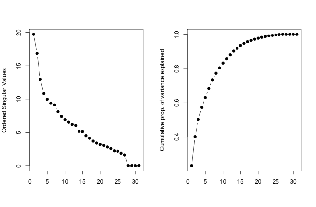
Figure E.2: The Singular Value spectrum for all outcomes

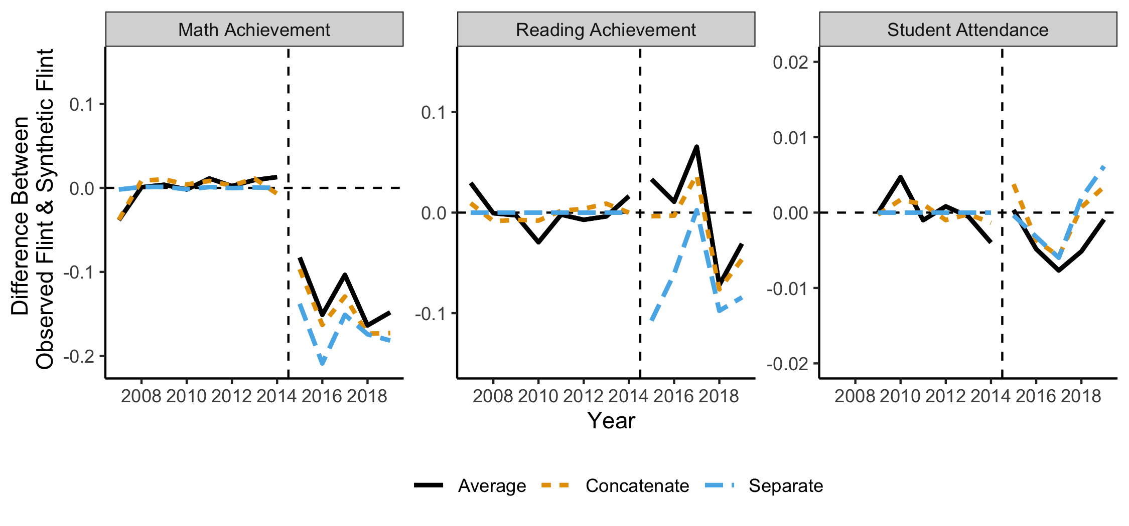
Figure E.3: Point estimates for the effect of the Flint water crisis using SCM, concatenate SCM, and average SCM, without including special needs. Each outcome is standardized using the series pre-treatment standard deviation.

References

• (1)
• Abadie (2021) Abadie, Alberto, “Using Synthetic Controls: Feasibility, Data Requirements, and Methodological Aspects,” Journal of Economic Literature, June 2021, 59 (2), 391–425.
• Abadie et al. (2010)   , Alexis Diamond, and Jens Hainmueller, “Synthetic Control Methods for Comparative Case Studies: Estimating the Effect of California’s Tobacco Control Program,” Journal of the American Statistical Association, 2010, 105 (490), 493–505.
• Abadie et al. (2015)   ,   , and   , “Comparative Politics and the Synthetic Control Method,” American Journal of Political Science, 2015, 59 (2), 495–510.
• Abadie and Gardeazabal (2003)    and Javier Gardeazabal, “The Economic Costs of Conflict: A Case Study of the Basque Country,” The American Economic Review, 2003, 93 (1), 113–132.
• Acemoglu et al. (2016) Acemoglu, Daron, Simon Johnson, Amir Kermani, James Kwak, and Todd Mitton, “The value of connections in turbulent times: Evidence from the United States,” Journal of Financial Economics, August 2016, 121 (2), 368–391.
• Agarwal et al. (2023) Agarwal, Anish, Devavrat Shah, and Dennis Shen, “Synthetic A/B Testing using Synthetic Interventions,” 2023.
• Amjad et al. (2019) Amjad, Muhammad, Vishal Misra, Devavrat Shah, and Dennis Shen, “mRSC: Multi-dimensional Robust Synthetic Control,” Proceedings of the ACM on Measurement and Analysis of Computing Systems, June 2019, 3 (2), 37:1–37:27.
• Arkhangelsky et al. (2021) Arkhangelsky, Dmitry, Susan Athey, David A. Hirshberg, Guido W. Imbens, and Stefan Wager, “Synthetic Difference-in-Differences,” American Economic Review, December 2021, 111 (12), 4088–4118.
• Athey et al. (2021) Athey, Susan, Mohsen Bayati, Nikolay Doudchenko, Guido Imbens, and Khashayar Khosravi, “Matrix Completion Methods for Causal Panel Data Models,” Journal of the American Statistical Association, 2021, 116 (536), 1716–1730.
• Ben-Michael et al. (2021) Ben-Michael, Eli, Avi Feller, and Jesse Rothstein, “The Augmented Synthetic Control Method,” Journal of the American Statistical Association, 2021, 116 (536), 1789–1803.
• Ben-Michael et al. (2022)   ,   , and   , “Synthetic controls with staggered adoption,” Journal of the Royal Statistical Society. Series B: Statistical Methodology, 2022, 84 (2), 351–381.
• Ben-Michael et al. (2023)   , David Arbour, Avi Feller, Alexander Franks, and Steven Raphael, “Estimating the effects of a California gun control program with multitask Gaussian processes,” The Annals of Applied Statistics, 2023, 17 (2), 985–1016.
• Billmeier and Nannicini (2013) Billmeier, Andreas and Tommaso Nannicini, “Assessing Economic Liberalization Episodes: A Synthetic Control Approach,” The Review of Economics and Statistics, 2013, 95 (3), 983–1001. Publisher: The MIT Press.
• Bohn et al. (2014) Bohn, Sarah, Magnus Lofstrom, and Steven Raphael, “Did the 2007 Legal Arizona Workers Act Reduce the State’s Unauthorized Immigrant Population?,” The Review of Economics and Statistics, May 2014, 96 (2), 258–269.
• Chernozhukov et al. (2019) Chernozhukov, Victor, Kaspar Wuthrich, and Yinchu Zhu, “An Exact and Robust Conformal Inference Method for Counterfactual and Synthetic Controls,” arXiv preprint arXiv:1712.09089, 2019.