Boson star head-on collisions with constraint-violating
and constraint-satisfying initial data

Abstract

Simulations of binary collisions involving compact objects require initial data that satisfy the constraint equations of general relativity. For binary boson star simulations it is common practice to use a superposition of two isolated star solutions to construct an approximate solution to the constraint equations. Such superposed data is simple to set up compared to solving these equations explicitly, but also introduces extra constraint violations in the time evolution. In this work we investigate how physical observables depend on the quality of initial data in the case of head-on boson star collisions. In particular we compare results obtained from data prepared using four different methods: the standard method to superpose isolated stars, a heuristic improvement to this superposition technique and two versions of this data where excess constraint violations were removed through a conformal thin-sandwich solver. We find that differences in the time evolutions are dominated by differences in the way the two superposition methods differ, whereas additionally constraint solving the superposed data has smaller impact. The numerical experiments are conducted using the pseudospectral code bamps. Our work demonstrates that bamps is a code suited for generating high accuracy numerical waveforms for boson star collisions due to the exponential convergence in the polynomial resolution of the numerical approximation.

I Introduction

With the first successful numerical relativity (NR) simulations of binary black hole (BH) collisions carried out [1, 2, 3, 4, 5], an industry for engineering waveform templates was founded which played a key role in the first gravitational wave (GW) detections [6, 7, 8]. The late inspiral part of GW templates are informed by NR simulations that solve an initial-boundary-value problem posed by a Cauchy formulation of the Einstein field equations (EFEs) of general relativity (GR). Essential to such simulations is the data described on an initial hypersurface which is then propagated forward in time to trace out a foliation of spacetime. This initial data should satisfy the Hamiltonian and momentum constraint equations of GR. If the initial data also involve matter models in the form of neutron stars (NSs) then one must also ensure that each star is initially in a state of quasi-equilibrium, i. e. this should account for effects like tidal deformations which are due to them inspiraling on each other at a finite distance. Given the difficulty of numerically solving the constraint equations to generate such physically plausible data a variety of formalisms and numerical methods have been developed for collisions in the context of BHs and NSs (see [9] for a review).

Almost a decade after the first GW detection the waveform template industry continues pushing forward analytical, computational, and phenomenological boundaries in order to keep up with the advancing detector technology and upcoming new experiments. Among these theoretical advances is also considerable effort to study compact objects described by exotic matter models that have been developed as dark matter candidates. Among those candidates are boson stars (BSs), which were first theorized in [10], and for which a variety of NR studies involving this particular model have been conducted. These studies uncovered a dynamical formation process termed gravitational cooling [11], as well as the anatomy of the GW signals from coalescences of such objects, see [12, 13, 14, 15] for head-on collisions and [16, 17, 18, 19, 20] for inspirals. Also see [21, 22, 23] for a review on BSs and variations thereof.

Most of today’s understanding of BS collisions comes from studies that use a superposition of isolated BSs as initial data which does not satisfy the constraint equations. Such data should be seen as approximate solutions to the constraint equations. Its use can be justified when it is explicitly verified that the error due to initial constraint violations does not dominate the overall error budget of the simulation. Only recently, work has started on refining the initial data construction for BS encounters. In [12, 13] a heuristically motivated correction to the commonly used method of superposition was developed by minimizing initial constraint violations, with some still remaining. To the best of our knowledge the first BS collisions using constraint solved data were reported in [24], which discussed BS head-on encounters only to calibrate the BAM code for evolutions of mixed NS-BS systems. In [25] a generic constraint solver for BS initial data was developed, which is an important contribution in order to catch up with the state-of-the-art initial data construction techniques commonly used for BH and NS simulations. Such constraint solved data was used to demonstrate that the collision of two non-rotating BSs can yield a rotating remnant [26].

As the sensitivity of the next generation of GW detectors increases, the accuracy demands on GW templates do as well. In anticipation of such a trend new NR codes are developed and existing NR codes are upgraded to improve the computational efficiency and the mathematical modeling of physical processes, e. g. BAM [27], GR-Athena++ [28], Dendro-GR [29], Einstein-Toolkit [30], ExaHyPE [31], GRChombo [32], Lean [33], MHDuet [34], NMesh [35], NRPy+ [36], SACRA [37], SpEC [38], SpECTRE [39], SPHINCS_BSSN [40], Spritz [41] (see also [42] for an extended list). Among these research efforts is also the bamps code [43, 44, 45, 46, 47, 48, 49, 50, 51] which employs a nodal pseudospectral (PS) discretization for the spatial representation of the solution. The promised efficiency and accuracy gain of a PS method can be demonstrated best for problems which admit smooth solutions. Since BSs lack a hard surface (or boundary) and no shock fronts are formed during mergers of such objects, which are common obstacles for BH and NS simulations that spoil smoothness, they represent an ideal testbed to develop and assess PS methods in the context of GR. Theoretically, the solution has exponential convergence when increasing the polynomial resolution of the PS approximations. This translates into a significantly reduced error budget that we attribute to the time evolution, assuming high enough resolution. Thus, for PS codes constraint violations in superposed initial data can in principle dominate the total error budget of our results, making the usage of superposed initial data ill-advised.

In this work we utilize the bamps code to perform binary BS head-on collisions with axisymmetry and reflection symmetry and investigate how physical observables extracted from these simulations depend on the quality of initial data. In particular, we compare results obtained from data that was prepared using four different methods: a simple superposition of isolated stars as defined in [12], the heuristic improvement to the simple superposition technique also reported in [12], and two versions of constraint-solved data obtained from a conformal thin-sandwich (CTS) solver and superposed free data. We then assess the differences between evolutions done with these data and the individual accuracy of each evolution by using a mixture of constraint monitors, global (and conserved) physical quantities, as well as gravitational waves, and (self-)convergence tests involving those quantities.

The rest of this work is structured as follows. First, we review the theory under study as well as the formulation of the equations of motion we use for the numerical simulations in Sec. II. In Sec. III a summary about earlier work on superposed initial data is given and we discuss how we construct constraint-solved data for the comparisons. Details on the computational setting are provided in Sec. IV and our numerical results are presented in Sec. V. A summary of our findings is provided in Sec. VI. In App. A and App. B we discuss details of our GW analysis and comment on a problem specific to head-on collisions and the reconstruction of the GW strain $h$ from the Newman-Penrose pseudoscalar $\Psi_{4}$. We use Latin indices starting from $a$ to denote spacetime components and Latin indices starting from $i$ to denote spatial components of tensors. We work in Planck units where $G=c=\hbar=1$ so that all variables are automatically dimensionless and we also set the scalar-field mass (defined below) to $\mu=1$. In App. C we show that this choice of $\mu$ does not limit the generality of our results, but instead corresponds to a particular rescaling of the variables.

II Theory

II.1 Action and equations of motion

This work is concerned with scalar BSs in GR. They are compact objects defined as solutions to the equations of motion in a theory in which the Einstein-Hilbert action for the gravitational field $g_{ab}$ is minimally coupled to a complex scalar field $\phi$ in the following way [21]

$$S=\int \differential^{4}x~{}\sqrt{-g}$$

$$\times\left(\frac{\tensor{[}^{(4)}]{R}{}}{16\pi}-\frac{1}{2}\left(g^{ab}\nabla_{a}\phi^{\ast}\nabla_{b}\phi+V(|\phi|^{2})\right)\right)\,,$$ (1)

where $g$ is the metric determinant, $\tensor{[}^{(4)}]{R}{}$ the Ricci scalar associated with $g_{ab}$ and $V(|\phi|^{2})$ is the scalar-field potential, and an asterisk refers to complex conjugation. The above action gives rise to the following equations of motion, known as the Einstein-Klein-Gordon (EKG) equations,

$$G_{ab} =8\pi T_{ab}\,,$$ (2)

$$\Box\phi =\phi\frac{\differential V}{\differential|\phi|^{2}}\,,$$ (3)

where $G_{ab}$ is the Einstein tensor, $\Box\equiv g^{ab}\nabla_{a}\nabla_{b}$ and the stress-energy tensor is given by

$$T_{ab} =\nabla_{(a}\phi^{\ast}\nabla_{b)}\phi-\frac{1}{2}g_{ab}\left(g^{cd}\nabla_{c}\phi^{\ast}\nabla_{d}\phi+V(|\phi|^{2})\right)\,.$$ (4)

BSs can come in different flavors determined by the form of the potential $V(|\phi|^{2})$. In this work we restrict ourselves to mini BSs for which the potential is that of a massive free scalar field,

$$V(|\phi|^{2})=\mu^{2}|\phi|^{2}\,,$$ (5)

where $\mu$ is the scalar field’s mass. For the rest of this work we set $\mu=1$.

II.2 3+1 decomposition

The basis for NR simulations is laid by a covariant 3+1 decomposition of the spacetime metric $\tensor{g}{{}_{a}{}_{b}}$, often written in the form [52]

$$g_{ab}\differential x^{a}\differential x^{b}=-\alpha^{2}\differential t^{2}+\gamma_{ij}(\differential x^{i}+\beta^{i}\differential t)(\differential x^{j}+\beta^{j}\differential t)\,.$$ (6)

The variables $\alpha$, $\beta^{i}$, $\gamma_{ij}$ and $K_{ij}$ are called the lapse, shift, spatial metric and extrinsic curvature, respectively, and are referred to as the 3+1 variables. Within this framework the EFEs are rewritten accordingly and this unveils the so-called Hamiltonian and momentum constraint equations (from here on only referred to as constraint equations) as part of this system of nonlinear PDEs [52],

$$\mathcal{H} :=R+K^{2}-K_{ij}K^{ij}-16\pi\rho=0\,,$$ (7)

$$\mathcal{M}^{i} :=D_{j}(K^{ij}-\gamma^{ij}K)-8\pi S^{i}=0\,,$$ (8)

where $R$ and $K_{ij}$ are the Ricci scalar and extrinsic curvature associated with $\gamma_{ij}$ and a spatial hypersurface $\Sigma$ that is embedded in the surrounding spacetime $(\mathcal{M},\tensor{g}{{}_{a}{}_{b}})$. The quantities $\rho=n^{a}n^{b}T_{ab}$ and $S^{i}=-\gamma^{ia}n^{b}T_{ab}$ are projections of the stress-energy tensor $T_{ab}$ onto $(\Sigma,\tensor{\gamma}{{}_{i}{}_{j}})$, where $n^{a}$ is the unit normal vector to $\Sigma$ and $\gamma^{ia}=g^{ia}+n^{i}n^{a}$. These equations constrain the fields $(\gamma_{ij},K_{ij})$ of a time slice $\Sigma$ such that the embedding of $(\Sigma,\gamma_{ij},K_{ij})$ in $(\mathcal{M},\tensor{g}{{}_{a}{}_{b}})$ is compatible with the covariant decomposition of the EFEs.

The remainder of the decomposition of the EFEs is complemented by how $\gamma_{ij}$ and $K_{ij}$ develop away from the initial hypersurface $\Sigma_{0}$. Augmenting these equations with conditions on how the variables $\alpha$ and $\beta^{i}$ evolve completes the system of nonlinear PDEs we aim to solve. In this work we utilize the generalized harmonic gauge (GHG) formulation of the EFEs [43, 53]

$$\partial_{t}\tensor{g}{{}_{a}{}_{b}} =\beta^{i}\partial_{i}\tensor{g}{{}_{a}{}_{b}}-\alpha\tensor{\Pi}{{}_{a}{}_{b}}+\gamma_{1}\beta^{i}\tensor{C}{{}_{i}{}_{a}{}_{b}}\,,$$ (9)

$$\begin{split}\partial_{t}\tensor{\Pi}{{}_{a}{}_{b}}&=\beta^{i}\partial_{i}\tensor{\Pi}{{}_{a}{}_{b}}-\alpha\gamma^{ij}\partial_{i}\tensor{\Phi}{{}_{j}{}_{a}{}_{b}}+\gamma_{1}\gamma_{2}\beta^{i}\tensor{C}{{}_{i}{}_{a}{}_{b}}\\ &\quad+2\alpha g^{cd}\left(\gamma^{ij}\tensor{\Phi}{{}_{i}{}_{c}{}_{a}}\tensor{\Phi}{{}_{j}{}_{d}{}_{b}}-\tensor{\Pi}{{}_{c}{}_{a}}\tensor{\Pi}{{}_{d}{}_{b}}-g^{ef}\tensor{\Gamma}{{}_{a}{}_{c}{}_{e}}\tensor{\Gamma}{{}_{b}{}_{d}{}_{f}}\right)\\ &\quad-2\alpha\left(\tensor{\nabla}{{}_{(}{}_{a}}\tensor{H}{{}_{b}{}_{)}}+\gamma_{4}\tensor{\Gamma}{{}^{c}_{a}{}_{b}}\tensor{C}{{}_{c}}-\frac{1}{2}\gamma_{5}\tensor{g}{{}_{a}{}_{b}}\Gamma^{c}\tensor{C}{{}_{c}}\right)\\ &\quad-\frac{1}{2}\alpha n^{c}n^{d}\tensor{\Pi}{{}_{c}{}_{d}}\tensor{\Pi}{{}_{a}{}_{b}}-\alpha n^{c}\gamma^{ij}\tensor{\Pi}{{}_{c}{}_{i}}\tensor{\Phi}{{}_{j}{}_{a}{}_{b}}\\ &\quad+\alpha\gamma_{0}\left(2\tensor{\delta}{{}^{c}_{(a}}\tensor{n}{{}_{b)}}-\tensor{g}{{}_{a}{}_{b}}n^{c}\right)\tensor{C}{{}_{c}}\\ &\quad-16\pi\alpha\left(T_{ab}-\frac{1}{2}g_{ab}\tensor{T}{{}^{c}_{c}}\right)\,,\end{split}$$ (10)

$$\begin{split}\partial_{t}\tensor{\Phi}{{}_{i}{}_{a}{}_{b}}&=\beta^{j}\partial_{j}\tensor{\Phi}{{}_{i}{}_{a}{}_{b}}-\alpha\partial_{i}\tensor{\Pi}{{}_{a}{}_{b}}+\gamma_{2}\alpha\tensor{C}{{}_{i}{}_{a}{}_{b}}\\ &\quad+\frac{1}{2}\alpha n^{c}n^{d}\tensor{\Phi}{{}_{i}{}_{c}{}_{d}}\tensor{\Pi}{{}_{a}{}_{b}}+\alpha\gamma^{jk}n^{c}\tensor{\Phi}{{}_{i}{}_{j}{}_{c}}\tensor{\Phi}{{}_{k}{}_{a}{}_{b}}\,,\end{split}$$ (11)

where the evolved variables are the metric $g_{ab}$ and the time reduction variable $\Pi_{ab}=-n^{c}\partial_{c}g_{ab}$, $\Gamma^{a}=g^{bc}\tensor{\Gamma}{{}^{a}_{b}{}_{c}}$ and $\Gamma_{abc}=g_{ad}\tensor{\Gamma}{{}^{d}_{b}{}_{c}}$ are the Christoffel symbols associated with $g_{ab}$. We would like to point out the extra minus sign in the definition of $\Pi_{ab}$ which was previously missing in [48] due to a typo. The spatial reduction variable $\Phi_{iab}$ is associated with the reduction constraint $C_{iab}=\partial_{i}g_{ab}-\Phi_{iab}=0$ and

$$C_{a}=H_{a}+\Gamma_{a}=0$$ (12)

is the harmonic constraint, where $H_{a}$ is a gauge source function. Here we choose the gauge source function introduced in [54] with $R(t)=W(x^{i})=1$. The constraint damping parameters are fixed to be $\alpha\gamma_{0}=1/10$, $\gamma_{1}=-1$, $\alpha\gamma_{2}=1$ and $\gamma_{4}=\gamma_{5}=1/2$. The above evolution equations are implemented in our numerical relativity code bamps and more details on the computational setup are discussed in Sec. IV.

To reduce the Klein-Gordon equation (3) to first order we introduce the reduction variables $\Pi=n^{a}\partial_{a}\phi$, $\Phi_{i}=\partial_{i}\phi$ and the spatial reduction constraint $B_{i}:=\partial_{i}\phi-\Phi_{i}$. The reduced system of equations is then of the form

$$\partial_{t}\phi =\alpha\Pi+\beta^{i}\Phi_{i}\,,$$ (13)

$$\partial_{t}\Pi =\beta^{i}\partial_{i}\Pi$$ (14)

$$+\gamma^{ij}\left(\Phi_{j}\partial_{i}\alpha+\alpha\partial_{i}\Phi_{j}-\alpha{}^{(3)}\Gamma^{k}{}_{ij}\Phi_{k}\right)$$

$$+\alpha\Pi K+\sigma\beta^{i}B_{i}\,,$$

$$\partial_{t}\Phi_{i} =\Pi\partial_{i}\alpha+\alpha\partial_{i}\Pi+\Phi_{j}\partial_{i}\beta^{j}$$ (15)

$$+\beta^{j}\partial_{j}\Phi_{i}+\sigma\alpha B_{i}\,.$$

The evolved variables are $\phi$, $\Phi_{i}$ and $\Pi$. ${}^{(3)}\tensor{\Gamma}{{}^{k}_{i}{}_{j}}$ refer to the Christoffel symbols associated with $\gamma_{ij}$ and $\sigma$ is a damping parameter which we set in all our simulations such that $\alpha\sigma=1$, equivalent to our treatment of $\gamma_{2}$.

III Initial data

III.1 Binary boson star initial data from superposition of isolated stars

The construction of initial data for simulations of compact binary objects requires finding a solution $(\gamma_{ij},K_{ij})$ to the geometric constraints (7) and (8) on an initial time slice $\Sigma_{0}$, while simultaneously also preparing the matter variables $\rho$ and $S^{i}$ in a state of quasi-equilibrium determined through auxiliary conditions. In the following discussion we neglect the latter aspect and focus only on the geometric constraints, but we revisit it briefly below. What defines physically plausible initial data is in general not a question with a simple answer. The basis for binary data construction is the existence of isolated star solutions, which are often assumed to be at least axisymmetric and, thus, simple to obtain numerically. Unfortunately, the assumption of a star being in isolation is, in principle, in contradiction with a star partaking in a binary collision, unless they are displaced by an infinite distance. On a physical basis this is clear, because the gravitational pull of one star will be felt by its companion, causing tidal deformations of it and, hence, influencing its gravitational potential, which in turn modifies the initial star through its own tidal forces. This is also reflected by the nonlinearity of the constraint equations which in general prevents the construction of new solutions as simple combinations of isolated single star solutions – commonly referred to as superposition.

As can be straightforwardly shown, the constraint equations, if satisfied at one instant of time and evolved exactly, will continue to hold at all times. Failing to satisfy these constraints does not necessarily cause crashes in numerical simulations, but results that do so are not solutions to the EFEs. Realizing that NR can only ever produce approximate numerical solutions to the continuum EFEs, any numerical result will inevitably violate the constraints to some degree. The goal of NR is to construct successive numerical approximations in such a way that constraint violations, as well as the evolved fields and other analysis quantities, show a controlled convergence trend towards the continuum EFEs in the limit of infinite resolution. We emphasize that violations occurring in time evolutions do not solely arise from the failure of the initial data to satisfy the constraints, but can e. g. also grow dynamically through numerical errors due to insufficient resolution, the appearance of (coordinate) singularities or other pathologies. In fact, constraint violations associated with the initial data quality are conceptually even simpler to control, because the mathematical problem of solving the constraint equations for the initial data is completely decoupled from solving the free evolution equations. Because of that, dedicated codes have been developed to tackle the initial data problem in GR (see [9] for a review of methods for BH and NS binaries, see [26] for a constraint solver for BS binaries).

Solving the constraint equations is a difficult task. Using instead a superposition of isolated single star solutions presents itself as an attractive shortcut to constructing initial data that solve the constraints approximately. In studies that use such data it is often argued that the approximation is accurate enough when the inherited constraint violations are at most of the same order as the error budget of the time evolutionary part of a numerical code [16]. Such an argument can be supported with convergence studies to demonstrate that the numerical results approximate solutions up to a controlled error, provided that one commits to routinely verify that the above premise is satisfied. In the case of BS simulations superposed data has been used many times before as starting points for head-on and inspiraling binary collisions [16, 15, 17, 18, 19, 20, 12, 13, 14]. The same technique has also been employed for collisions involving other exotic matter models like Proca stars [55, 56, 57], $\ell$-boson stars [58], dark boson stars [59], axion stars [60], neutron stars with bosonic cores [61] as well as mixed mergers of an axion star and a black hole [62], a neutron star and an axion star [63, 62], and a boson star and a black hole [64, 65].

Focusing on pure scalar BS simulations, one recipe employed in the literature to construct superposed data can be summarized as follows. Let $\gamma_{ij}^{A}$, $K_{ij}^{A}$, $\alpha_{A}$ and $\beta_{A}^{i}$ denote the 3+1 variables of spacetime and let $\phi_{A}$ and $\Pi_{A}$ denote the scalar-field variables of star $A$, likewise for star $B$. A simple superposition (SSP) initial data construction involving stars $A$ and $B$ is then given by [12]

$$\gamma_{ij} =\gamma_{ij}^{A}+\gamma_{ij}^{B}-\delta_{ij}\,,$$ (16)

$$K_{ij} =\gamma_{m(i}\left(K_{j)n}^{A}\gamma_{A}^{nm}+K_{j)n}^{B}\gamma_{B}^{nm}\right)\,,$$ (17)

$$\phi =\phi_{A}+\phi_{B}\,,$$ (18)

$$\Pi =\Pi_{A}+\Pi_{B}\,,$$ (19)

where the data of the isolated stars is boosted such that the superposition mimics a binary configuration where each star carries initial momenta. This boosting itself is readily done through Galilean or Lorentz boost transformations [16, 12]. A slight variation of this recipe has been used in other studies that fueled many important contributions to the field [16, 15, 17, 18, 19].

The above construction disregards the constraint equations. Consequently, it comes as no surprise that in [12] it has been demonstrated that the scalar-field amplitude can admit artificial modulations. These effects can be strong enough to trigger premature BH collapse in encounters of BSs with a solitonic potential. Similar results were reported earlier in [66] for the case of compact real-scalar solitons (oscillatons). To tackle these symptoms, the same authors came up with a heuristically motivated improvement to the SSP construction, guided by minimizing initial constraint violations, which we refer to as the constant volume element (CVE) construction. Since the ansatz (16) alters the volume form inside a star depending on the displacement of the companion star, it was adjusted to

$$\gamma_{ij} =\gamma_{ij}^{A}+\gamma_{ij}^{B}-\gamma_{ij}^{A}(x_{B})\,.$$ (20)

Here $\gamma_{ij}^{A}(x_{B})$ refers to the constant value of the components of the induced metric of star A, $\gamma_{ij}^{A}$, evaluated at the center of star B, $x_{B}$. Note that in the case of equal mass BS binary systems we have $\gamma_{ij}^{A}(x_{B})=\gamma_{ij}^{B}(x_{A})$. Consequently, the above ensures that $\gamma_{ij}(x_{A})=\gamma_{ij}^{A}(x_{A})$ and likewise for B, hence, it approximately restores the volume element form around each star’s center to the value of an isolated star. This simple correction was enough to cure premature BH collapse, but at the same time, the correction led to qualitative changes in the emitted GW signals [12]. Recently, [13] generalized the CVE construction to also work with unequal mass binaries.

[width=0.95]figs/constraint-id-hyperspace-v4.4-no-formulae.pdf

Figure 1: Schematic representation of the space of initial data (orange) and of constraint-satisfying data (green). The red dots correspond to superposed initial data constructed with the SSP or CVE technique. The blue dots correspond to a projection of SSP and CVE data (in this work we use a CTS constraint solver for this, see text) onto the space of constraint-satisfying data. Dashed lines indicate the trajectories of the data when evolved through an evolution system with a damping scheme. Initially constraint-violating data might end up a distance $\epsilon$ displaced (yellow) and never reach the space of constraint-satisfying data.

We now have two methods at our disposal to construct superposed initial data and one might ask which of those is preferred, given that their time evolutions can yield different physical results. One might be inclined to prefer the CVE construction, because it reduces constraint violations and cures premature BH collapse. But whether these differences are only caused by the improvement of the constraint violations or are perhaps primarily due to changes in physical characteristics of the initial data, like for instance the local energy density, is yet unclear. To further illustrate this point consider Fig. 1 which schematically shows how constraint violations (measured in some norm) associated with initial data might propagate in time, when using an evolution system with a built-in constraint damping scheme like GHG. The CVE construction provides initial data with less constraint violations than the initial data constructed with the SSP technique, which is indicated by the two red dots lying on the space of all initial data (orange) at $t=0$ while also being displaced vertically from the space of constraint-satisfying data (green). The two blue dots, on the other hand, represent two different initial data sets (which are constructed in this work) where all excess constraint violations (ignoring numerical error) were removed from the superposed initial data. Performing time evolutions will then trace out the dashed trajectories, which indicate that constraint-satisfying initial data remain constraint-satisfying throughout the evolution. Contrary to this, evolutions starting from superposed initial data will only gradually in time approach the space of constraint-satisfying data. Note that the seemingly attractive character of the space of constraint-satisfying data is usually due to two factors: 1) the use of modified evolution equations that include constraint damping terms and 2) the possibility that constraint violations can propagate and eventually leave the computational domain through a boundary. Furthermore, there is no guarantee that initially-constraint-violating data is going to converge with increasing resolution towards constraint-satisfying data at late times. Instead one should expect some excess violations to remain also for late times $t$, which is illustrated by the trajectories ending up on the yellow space that is displaced by $\epsilon$ from the space of constraint-satisfying data. Besides this vertical displacement at late times, it is also unclear whether two trajectories that emanated from two initial data sets that are based on the same superposition, but where one is constraint-violating and one constraint-satisfying, will end up close to each other. Below we investigate the qualitative behavior of the sketched trajectories for the case of selected binary BS configurations and study their behavior when varying numerical resolution.

The above discussion as well as the rest of this work does not account for the problem of the progenitors not being initially in a state of quasi-equilibrium, which is done to ease this comparison. We want to highlight that the constraint equations need to be satisfied regardless of the matter model considered to study solutions to the EFEs, and matter fields enter these equations only as source terms. On the other hand, the equations of motion of most matter models, including BSs, do not provide any constraints, meaning that, in principle, arbitrary matter configurations could be used as initial data, provided the metric fields are adjusted to satisfy the geometric constraints. Instead, one requires additional assumptions to define a quasi-equilibrium, e. g. the existence of a helical Killing vector field for binary inspiral configurations, as well as an understanding of the matter model to derive (elliptic) equations that equilibrate their fields accordingly. Special attention has been given to the latter aspect of initial data construction in the BH and NS literature, see [67, 68, 69, 52]. First work in this direction for binary BSs has started only recently in [25] and we leave it to future work to further study the importance of this facet.

In the next section we examine one possibility to remove excess constraint violations from SSP and CVE initial data by numerically solving the constraint equations using a CTS solver, where the free data is constructed from the SSP and CVE data. Subsequently, we perform time evolutions using this data in order to answer the question of whether differences in physical observables between SSP and CVE initial data are caused by constraint violations. Along the way we also conduct convergence studies to assess the quality of our numerical results.

III.2 Constraint satisfying binary boson star initial data

Constraint satisfying binary BS initial data has been constructed before in [24] as well as in [26, 25] and was an important ingredient in demonstrating that the collision of two non-rotating BSs can form a rotating remnant. Below we follow a similar procedure by using the CTS formulation of the Hamiltonian and momentum constraints (7) and (8), which read [70]

$$\bar{D}^{2}\psi -\frac{1}{8}\psi\bar{R}-\frac{1}{12}\psi^{5}K^{2}+\frac{1}{8}\psi^{-7}\bar{A}_{ij}\bar{A}^{ij}$$

$$=-2\pi\psi^{5}\rho\,,$$ (21)

$$(\bar{\Delta}_{L}\beta)^{i} -(\bar{L}\beta)^{ij}\bar{D}_{j}\log(\bar{\alpha})$$

$$=\bar{\alpha}\bar{D}_{j}(\bar{\alpha}^{-1}\bar{u}^{ij})+\frac{4}{3}\bar{\alpha}\psi^{6}\bar{D}^{i}K$$

$$+16\pi\bar{\alpha}\psi^{10}S^{i}\,,$$ (22)

where

$$\bar{A}^{ij}=\frac{1}{2\bar{\alpha}}((\bar{L}\beta)^{ij}-\bar{u}^{ij})\,.$$ (23)

The above constitute a system of four elliptic PDEs for the conformal factor $\psi$ and the components of the shift vector $\beta^{i}$, where $\bar{D}$ is the covariant derivative associated with the conformal metric $\bar{\gamma}_{ij}$, $\bar{R}$ is the Ricci scalar associated with $\bar{\gamma}_{ij}$ and [52]

$$(\bar{\Delta}_{L}\beta)^{i} =\bar{D}^{2}\beta^{i}+\frac{1}{3}\bar{D}^{i}(\bar{D}_{j}\beta^{i})+\tensor{\bar{R}}{{}^{i}_{j}}\beta^{j}\,,$$ (24)

$$(\bar{L}\beta)^{ij} =\bar{D}^{i}\beta^{j}+\bar{D}^{j}\beta^{i}-\frac{2}{3}\bar{\gamma}^{ij}\bar{D}_{k}\beta^{k}\,,$$ (25)

are the conformal versions of the vector Laplacian and vector gradient applied to $\beta^{i}$, respectively. Once a solution for $\psi$ and $\beta^{i}$ is known, the remaining 3+1 variables can be recovered from

$$\gamma_{ij} =\psi^{4}\bar{\gamma}_{ij}\,,$$ (26)

$$K_{ij} =\psi^{-2}\bar{A}_{ij}+\frac{1}{3}\gamma_{ij}K\,,$$ (27)

$$\alpha =\psi^{6}\bar{\alpha}\,.$$ (28)

Equations (21) and (22) need to be complemented with freely specifiable data for $\bar{\gamma}_{ij}$, its time derivative $\bar{u}_{ij}:=\partial_{t}\bar{\gamma}_{ij}$, the trace of the extrinsic curvature $K$ and the conformal lapse $\bar{\alpha}$. Because we want to test the influence of eliminating constraint violations from superposed initial data, denoted by $(\gamma_{ij}^{(\textrm{sup})},K^{(\textrm{sup})})$, we use that data to setup the free data for the CTS formulation, following [71],

$$\bar{\gamma}_{ij} =\gamma_{ij}^{(\textrm{sup})}\,,$$ (29)

$$\bar{u}_{ij} =u_{ij}^{(\textrm{sup})}\,,$$ (30)

$$\bar{u}^{ij} =\bar{\gamma}^{ik}\bar{\gamma}^{jl}\left(\bar{u}_{kl}^{(\textrm{sup})}-\frac{1}{3}\bar{\gamma}^{mn}\bar{u}_{mn}\bar{\gamma}_{kl}\right)\,,$$ (31)

$$K =K^{(\textrm{sup})}\,,$$ (32)

$$\bar{\alpha} =\alpha^{(\textrm{sup})}=\det(\gamma_{ij}^{(\textrm{sup})})^{-1/6}\,,$$ (33)

$${\beta^{(\textrm{sup})i}} =0\,,$$ (34)

and

$$u_{ij}^{(\textrm{sup})}=\partial_{t}\gamma_{ij}^{(\textrm{sup})}=-2\alpha^{(\textrm{sup})}K^{(\textrm{sup})}+\mathcal{L}_{\boldsymbol{\beta}^{(\textrm{sup})}}\gamma_{ij}^{(\textrm{sup})}\,,$$ (35)

where $\mathcal{L}_{\boldsymbol{\beta}^{(\textrm{sup})}}$ denotes the Lie transport along the shift vector $\beta^{(\textrm{sup})i}$ of the superposed data. The choices (33) and (34) were adopted from [12]. Note that the difference in sign in (31) when compared to [71] is due to a difference in notation (see App. E).

The metric variables $\gamma_{ij}^{(\textrm{sup})}$, $K^{(\textrm{sup})}$, $\alpha^{(\textrm{sup})}$ and $\beta^{(\textrm{sup})i}$ are given by (16), (17), (33) and (34) or (20), (17), (33) and (34), respectively. The matter source terms $\rho$ and $S^{i}$ are computed from $\gamma_{ij}^{(\textrm{sup})}$, $K^{(\textrm{sup})}$, $\alpha^{(\textrm{sup})}$, $\beta^{(\textrm{sup})}$ and $T_{ab}$ given by (4). The construction of the latter is done by using the metric variables as well as the matter variables $\phi$ and $\Pi$ as given by (19) and (20). Note that, although the way the scalar field is superposed by (18) and (19) is the same between the SSP and CVE method, the difference in the superposition of the induced metric $\gamma_{ij}$, given by (16) and (20), then also translates into differences in the stress-energy tensor between these two constructions.

The numerical solution of (21) and (22) is obtained using the hyperbolic relaxation method [47], which is available inside the bamps code. For the CTS solver we use Robin boundary conditions to impose the asymptotic behavior [47]

$$\alpha=\psi =1+\mathcal{O}(r^{-1})\,, \beta^{i} =\mathcal{O}(r^{-1})\,.$$ (36)

To set up the free data for the solver we proceed as follows: first, we compute spherically symmetric stationary solutions of isolated BSs; two such stars are then each boosted by a parameter $v$ using a Lorentz transformation. For both of these steps we follow closely the algorithms given in [12] (also see App. D). We then use these stars to construct SSP or CVE initial data following the algorithms given in subsection III.1. These SSP and CVE data are then used together with (29)-(35) to set up the free data and sources for solving the CTS equations (21) and (22). As an initial guess for the CTS solver we use

$$\psi =1\,, \beta^{i} =0\,.$$ (37)

The hyperbolic relaxation of the CTS solver terminates once the sum of the $L^{1}$ norm of the right-hand side (RHS) of equations (21) and (22) is smaller than $1/10$th the sum of the $L^{1}$ norm of the residuals of those equations, or when the $L^{1}$ norm of the residual of the equations falls below $10^{-8}\times\#N_{\text{DOF}}\times 4$, where $N_{\text{DOF}}$ is the total number of grid points on the target resolution. The resulting constraint-satisfying data is referred to as CTS+SSP and CTS+CVE data for the rest of this work.

When we consider evolutions of constraint-satisfying data below, for which we fix the grid structure and the polynomial resolution $n$ in each cell, but we vary $n$ between different runs, the initial data is computed using the hyperbolic relaxation method on the very same grid structure and with the same polynomial resolution. In particular, no extra interpolation step is needed to convert the solution of the bamps internal CTS solver into initial data for the evolution.

For evolutions of superposed data we utilize (33) and (34) as initial data for $\alpha$ and $\beta^{i}$. For the case of constraint-solved data we use instead the solutions obtained from the CTS equations (21), (22) and the relation (28) to set up $\alpha$ and $\beta^{i}$.

IV Computational setup

Table 1: Summary of the grid configuration used for all the results presented in this work. The highest resolved configuration ($n=21$ and 48 outer shells) uses $423360$ degrees of freedom (already accounting for axisymmetry and reflection symmetry).

Parameter	value	description
grid.cube.max	80	1/2 side length of inner cube
grid.sub.xyz	16	number of subdivisions in inner cube
grid.cubedsphere .max.x	160	outer radius of cube-to-sphere patch
grid.cubedsphere .sub.x	8	number of radial subdivisions in cube-to-sphere patch
grid.sphere .max.x	[400,800]	outer radius of sphere path
grid.sphere .sub.x	[24,48]	number of radial subdivisions in sphere patch
grid.dtfactor	0.25	CFL factor
grid.cartoon	xz	double cartoon method
grid.reflect	z	reflection symmetry across $z=0$ plane
grid.n.xyz	$n:=$ [7,9,11,13, 15,17,19,21]	number of points per grid and per dimension

bamps [44, 45, 46, 47, 48] is a numerical code that has been used successfully to study critical collapse [43, 51, 50, 49]. It uses a pseudospectral collocation method for the spatial discretization of the EFEs and an explicit fourth-order Runge-Kutta time stepping algorithm. bamps utilizes distributed memory parallelization based on the Message Passing Interface (MPI) standard and, recently, has been complemented with an adaptive mesh refinement (AMR) feature [48]. However, in this work we do not make use of the AMR feature in order to facilitate the comparison. This means that we are using the same static computational grid structure between different simulations and we use the same polynomial resolution in all grid cells. In Table 1 we summarize important parameters of our computational setup.

The GHG formulation (9)-(11) of the EFEs to evolve the gravitational field and the first order reduction of the Klein-Gordon equation (13)-(15) to evolve the complex scalar field are implemented in bamps. The code employs radiation-controlling and constraint-preserving boundary conditions as described in [43, 72, 53]. The scalar field uses a maximally dissipative boundary condition on the physical degrees of freedom and constraint preserving boundary conditions for the reduction constraints [46]. We note that these boundary conditions were initially designed for real massless scalar-field evolutions and were adapted for this study to also work for massless complex scalar fields. In particular, they do not account for a scalar-field potential $V(|\phi|^{2})$, which is likely the cause for some of the artifacts we report below. We leave it for future work to improve these conditions. After extensive testing we found that the combination of the GHG formulation with the constraint damping parameters as given in Sec. II together with the grid parameters reported in Table 1 and the above boundary conditions allow us to perform long-time stable and convergent evolutions of binary BS head-on collisions.

V Results

Table 2: Properties of the stationary, isolated and spherically symmetric mini BS solution that is used as the basis for all the binary BS initial data constructions presented in this work. The same configuration has been studied in [12]. $A_{\textrm{ctr}}$ is the central scalar-field amplitude, $\omega$ is the stationary angular frequency of the harmonic time dependence of the scalar field, $M_{\textrm{BS}}$ is the ADM mass of the system and $r_{99}$ is the radius in which $99\%$ of the ADM mass are contained. We use $M_{\textrm{BBS}}=2M_{\textrm{BS}}=0.79$ as an estimate for the initial ADM mass of the binary system.

Model	$A_{\textrm{ctr}}$	$\omega$	$M_{\textrm{BS}}$	$r_{99}$
mini1	0.0124	0.97(1)	0.39(5)	22.(6)

We focus exclusively on head-on collisions of equal mass mini BSs. Some of the key properties of the particular stationary and isolated BS solution we used as the basis for the initial data construction are summarized in Table 2. In the head-on configurations we study we vary the initial boost parameter $v$ as well as the initial separation $d$ between the stars. Similar configurations were discussed already in [12] and a slight variation thereof, with non-zero impact parameter, was investigated in [14]. All collisions for which we report results below culminate in a single perturbed and non-spinning BS remnant with zero bulk motion with respect to the coordinate origin and where the gravitational and scalar fields continue to oscillate. The latter process causes a continued emission of GWs and scalar-field radiation, which lasts for much longer than the head-on impact. The GWs emitted due to the oscillating remnant are referred to as the gravitational afterglow of BSs [14]. This afterglow radiation is characterized by an amplitude that is comparable with the GW burst that is due to the initial head-on impact. See Fig. 10 below for an example of GW afterglow obtained from a long-time evolution.

Besides the intended direct comparison of the initial data quality, we repeat some of the experiments reported in [12] to perform calibration tests with our NR code bamps, as it is the first time it is used for BS evolutions. Given that bamps employs a PS method for the spatial discretization of the fields, whereas [12] used the Lean code [33] and the GRChombo code [73, 32] which both work with finite-differencing methods, the presented results also provide an (indirect) benchmark between different numerical methods for the simulation of spacetimes with smooth matter fields.

To gauge differences in numerical evolutions for the comparison of constraint-satisfying and violating initial data one can use various quantities. Below we focus on a mixture of constraint monitors, global (and conserved) physical quantities, as well as local field values and gravitational waves. Studying these quantities also allows us to assess the accuracy and reliability of the PS scheme employed. This is important to our work, because the equations of motion of the matter (Klein-Gordon equation) can be rewritten to mimic a balance law (i. e. a conservation law with an inhomogeneity) for which a plethora of numerical methods have been developed in the computational fluid dynamics literature and are often employed in the context of general relativistic hydrodynamics simulations. On the other hand the PS method developed in [43] was solely designed to conserve energy within a particular approximation and so it is of interest to us to see how well the scheme can balance matter fields over long times.

During binary BS evolutions we compute:

1. The constraint monitor $\mathcal{C}_{\textrm{mon}}$ defined in [43]. It summarizes violations of the constraint subsystem of GHG, among which are the Hamiltonian and momentum constraints (7) and (8) as well as the harmonic gauge constraint (12). In the continuum limit $\mathcal{C}_{\textrm{mon}}=0$ throughout the evolution. In practice we observe non-zero values for $\mathcal{C}_{\textrm{mon}}$ and they serve as a proxy to gauge to which accuracy the EFEs can be solved.

2. The dynamical behavior of the stars and spacetime are monitored through the maximum of the scalar-field amplitude $A_{\textrm{max}}(t)$ and the value of the Ricci scalar at the coordinate origin $R(t,x=0)$. These quantities together with $\mathcal{C}_{\textrm{mon}}$ are used to distinguish physical signatures from numerical artifacts in our analysis.

3. The Noether charge associated with the global $U(1)$ symmetry of (1) is given by [21]

   $$N =\int_{V}\differential x^{3}~{}\sqrt{-g}j^{t}\,,$$ (38)

   $$j^{a} =\frac{i}{2}g^{ab}\left(\phi^{\ast}\nabla_{b}\phi-\phi\nabla_{b}\phi^{\ast}\right)\,,$$ (39)

   where $j^{a}$ is the Noether current and integration is performed over the whole computational domain $V$. $N$ can be related to the total number of bosonic particles [21, 74]. This quantity is also conserved, provided no matter leaves the domain through a boundary, and, thus, its time evolution allows to gauge the accuracy of the evolution of the Klein Gordon equation.

4. The ADM mass of the spacetime [52]

   $$M_{\textrm{ADM}} =\frac{1}{16\pi}\lim_{r\to\infty}\int_{\partial\Sigma_{r}}\differential S~{}\mathcal{N}^{k}\gamma^{ij}(\partial_{j}g_{ik}-\partial_{k}g_{ij})\,,$$ (40)

   where $\mathcal{N}^{m}$ is the outward pointing unit normal vector to a 2-hypersurface $\partial\Sigma_{r}$ of a spatial slice $\Sigma$. In theory, this quantity is conserved in time and we monitor its temporal evolution to benchmark our results. Note that the results of $M_{\textrm{ADM}}$ we report below were obtained without taking the limit $r\to\infty$ and instead computed at a finite radius. In this sense all references of $M_{\textrm{ADM}}$ in the following refer to an approximation of the ADM mass. In fact, this approximation of $M_{\textrm{ADM}}$ is also not necessarily conserved and can show a decrease in time, in particular when matter leaves the computational domain.

5. A total mass number [14]

   $$M_{\textrm{tot}} =\int_{V}\differential x^{3}\sqrt{\gamma}\rho\,,$$ (41)

   where $\rho=T_{\mu\nu}n^{\mu}n^{\nu}$ is the local energy density and integration is performed over the whole computational domain $V$. This is a coordinate dependent quantity and it is not necessarily conserved.

6. Gravitational radiation represented through the curvature pseudo-scalar field $\Psi_{4}$. This (or rather integrals thereof) is the only accessible observable with which binary BS encounters could be experimentally detected. In particular, we only focus on the dominant $l,m=2,0$ mode. We leave out a discussion of the GW strain $h$ due to unacceptably large uncertainties introduced in the reconstruction procedure, see App. A.

7. The radiated GW energy $E$ associated with $\Psi_{4,20}$ as recorded by an asymptotic observer over a fixed time interval. This quantity was also studied in [12] to analyze the behavior of the long-lived oscillating remnant. The error bars we provide account for errors due to finite resolution, errors in the extrapolation to null infinity and errors in the reconstruction of $E$ from $\Psi_{4,20}$. For details on this analysis see App. A.

8. The detector-noise-weighted Wiener product $W(\Psi_{4,20}^{(1)},\Psi_{4,20}^{(2)})$ between two GW signals. This quantity gives a measure of how similar two GWs are, while accounting for detector sensitivity. To evaluate $W$ one has to assume a value for scalar-field mass $\mu$ in order to convert the results to SI units. Because we use a noise-sensitivity curve of Advanced LIGO [75] to weight the Wiener product, we fix $\mu=1\times 10^{-11}~{}\text{eV}$ so that the frequency of the dominant component of the PSD of $\Psi_{4,20}$ falls into the most sensitive region of the detector, which is at $\mathcal{O}(100~{}\text{Hz})$ [76]. For details see App. B.

V.1 Constraint violations

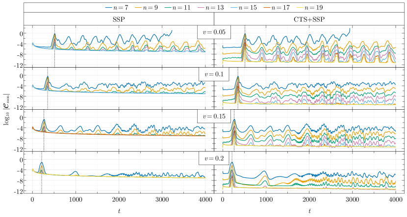
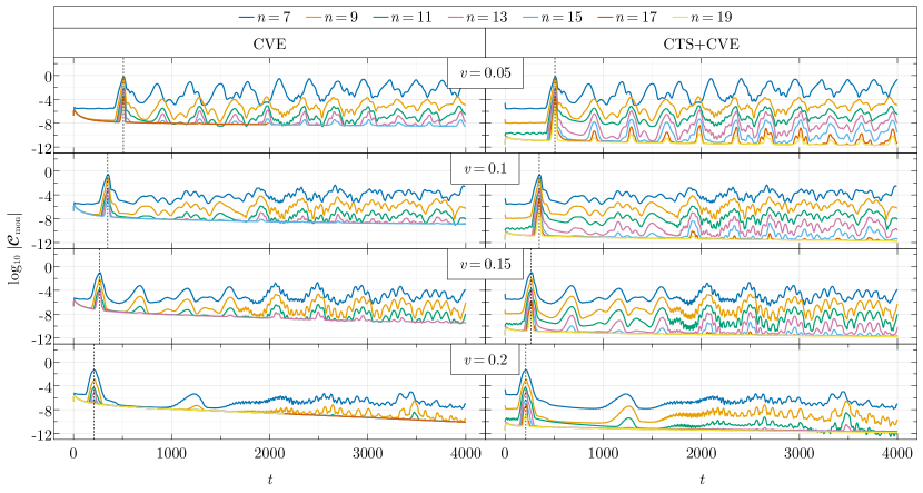
Figure 2: Side by side comparison of the time evolution of $\mathcal{C}_{\textrm{mon}}$ for simulations based on SSP data (left column) and CTS+SSP data (right column) for fixed initial separation $d=80$, varying resolutions and different values of the boost parameter $v=$ 0.05, 0.1, 0.15, 0.2 (from top to bottom). Vertical dashed lines indicate time of merger as determined by the time of the maximum value of $A_{\textrm{max}}(t)$ from the highest resolution.

Figure 3: Side by side comparison of the time evolution of $\mathcal{C}_{\textrm{mon}}$ for simulations based on CVE data (left column) and CTS+CVE data (right column) for fixed initial separation $d=80$, varying resolutions and different values of the boost parameter $v=$ 0.05, 0.1, 0.15, 0.2 (from top to bottom). Vertical dashed lines indicate time of merger as determined by the time of the maximum value of $A_{\textrm{max}}(t)$ from the highest resolution.

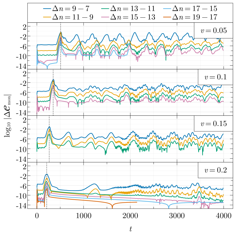
Figure 4: Self-convergence test of the constraint monitor $\mathcal{C}_{\textrm{mon}}$. Left Results obtained from evolutions of SSP data. Right Results obtained from evolutions of CVE data. The initial separation is fixed to $d=80$ and initial boost values are $v=$ 0.05, 0.1, 0.15, 0.2. Vertical dashed lines indicate time of merger as determined by the time of the maximum value of $A_{\textrm{max}}(t)$ from the highest resolution.

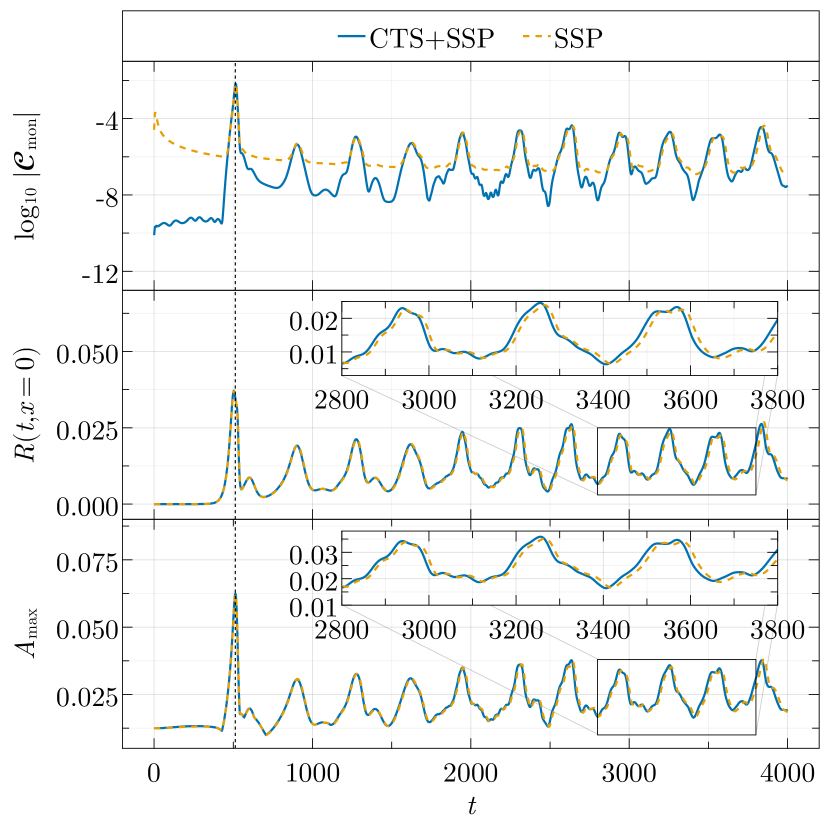
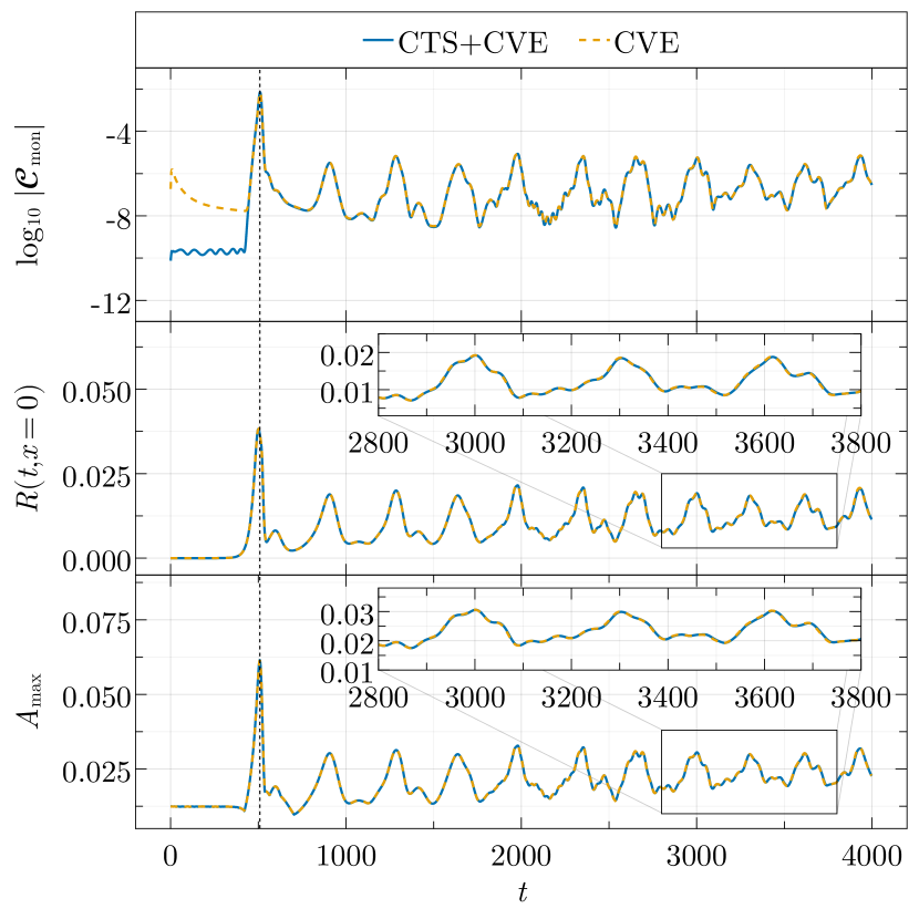
Figure 5: Direct comparison of evolution quantities $\mathcal{C}_{\textrm{mon}}$ (top), $R(t,x=0)$ (middle) and $A_{\textrm{max}}(t)$ (bottom) obtained from binary BS evolutions of superposed initial data (dashed) vs. constraint-solved data (solid). The stars were prepared with boost parameter $v=0.05$ and initial distance $d=80$ and polynomial resolution was $n=11$. Left Comparison between SSP data vs. and CTS+SSP data. Right Comparison between CVE vs. and CTS+CVE data. The vertical dashed lines indicate time of merger as determined by the time of the maximum value of $A_{\textrm{max}}(t)$.

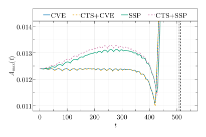
Figure 6: Direct comparison of $A_{\textrm{max}}(t)$ obtained from binary BS evolutions that used constraint-violating SSP and CVE data (solid) and constraint-satisfying CTS+SSP and CTS+CVE data (dashed). The stars were prepared with boost parameter $v=0.05$, initial distance $d=80$ and polynomial resolution was $n=11$. This is a zoomed in plot of the $A_{\textrm{max}}(t)$ results presented in Fig. 5. The vertical dashed and dotted lines indicate time of merger as determined by the time of the maximum value of $A_{\textrm{max}}(t)$ from the CTS+SSP and CTS+CVE data, respectively.

A comparison of the convergence behavior of $\mathcal{C}_{\textrm{mon}}$ obtained from runs that used SSP data vs. CTS+SSP data with initial separation $d=80$, boost parameters $v=0.05,0.1,0.15,0.2$ and varying polynomial resolutions $n$ is provided in Fig. 3.

First, we compare the values of $\mathcal{C}_{\textrm{mon}}$ at $t=0$ between the constraint-violating SSP data (left columns) and constraint-satisfying CTS+SSP data (right columns). The figure shows that all SSP evolutions start from an initial violation $\mathcal{C}_{\textrm{mon}}\approx 10^{-4}$, which is independent of the resolution and initial boost. On the other hand, the CTS+SSP data starts off at $\mathcal{C}_{\textrm{mon}}\approx 10^{-5}$ and decreases with $n$ and independent of $v$ to $\mathcal{C}_{\textrm{mon}}<10^{-10}$. Because we solve the CTS equations for each resolution $n$ separately, instead of solving them once for a high resolution and then using interpolation to obtain data on a lower resolution, this behavior of $\mathcal{C}_{\textrm{mon}}$ demonstrates that our CTS solver is capable of removing excess constraint violations with increased resolution.

Focusing on the time evolution of $\mathcal{C}_{\textrm{mon}}$ of CTS+SSP data, one observes a clear convergence pattern in resolution. We want to emphasize the rate by which $\mathcal{C}_{\textrm{mon}}$ decreases by pointing to the exponential improvement of $\mathcal{C}_{\textrm{mon}}$ from $10^{0}$ down to $10^{-12}$ while the polynomial resolution $n$ increases linearly in steps of two from 7 to 19 (see color coding in legend). For boost values $v=$ 0.1, 0.15 and 0.2 one observes that with resolutions $n\geq 15$ the violations are bounded by $\mathcal{C}_{\textrm{mon}}\lesssim 10^{-10}$ when $0\leq t\leq 4000$, except around the merger which occurs at $t\approx 350$, 260 and 210, respectively. For the runs using $v=0.05$ one would need to increase the resolution beyond $n=19$ to achieve the same level of violations in the afterglow signal, which is computationally well within reach even without AMR. Comparing now with the violations from evolutions of SSP data one can also see that $\mathcal{C}_{\textrm{mon}}$ decreases for all simulations independent of $v$. However, the results for $v=$ 0.05, 0.1 and 0.15 show that this trend eventually halts when $n\gtrsim 13$ and for $v=0.2$ no improvement occurs beyond $n=11$ in the afterglow. From this we conclude that evolutions of non-constraint-solved SSP data bear a residual constraint violation $\mathcal{C}_{\textrm{mon}}\gtrsim 10^{-8}$ when $0\leq t\leq 4000$ for this configuration in our code. Note that this result does not imply that these evolutions are not convergent, because a numerical value of order $\mathcal{O}(10^{-8})$ is usually not regarded as numerically zero. Instead one must treat this data series as a series that approaches a non-zero residual value and conduct a self-convergence test, which is done further below.

Studying now the behavior of $\mathcal{C}_{\textrm{mon}}$ around merger one observes that the constraint monitor continues to improve with increasing $n$, even when $\mathcal{C}_{\textrm{mon}}$ was already saturated away from merger. This behavior is independent of the boost parameter $v$ and occurs for SSP and CTS+SSP data. The reason for this is that the merger phase typically involves higher field amplitudes and gradients compared to less extreme field configurations before and after merger, which translates into a need for locally higher polynomial approximations to resolve the solutions accurately, due to aliasing effects in the PS expansion being amplified by the nonlinearity of the EFEs. As a side note we mention that the use of AMR could potentially bring down these constraint violations around merger to the same level away from the merger, while at the same time improve computational efficiency by distributing the available resources where numerical resolution is needed. We leave this test to future work as it will certainly become of relevance for inspiral simulations.

Fig. 3 shows the same comparison of $\mathcal{C}_{\textrm{mon}}$, but for evolutions that started with constraint-violating CVE data vs. constraint-satisfying CTS+CVE data and the same initial distance and boost parameters. The overall behavior of the results is similar to the one from Fig. 3: at $t=0$ the CVE data comes with an initial violation $\mathcal{C}_{\textrm{mon}}\approx 10^{-6}$ that is independent of $n$ and $v$, whereas the CTS+CVE data starts at $\mathcal{C}_{\textrm{mon}}\approx 10^{-5}$ and continuously decreases with increasing resolution to $\mathcal{C}_{\textrm{mon}}<10^{-10}$. The time evolution of CTS+CVE data also displays a convergence pattern with exponential decrease when increasing $n$, and the constraint violations are reduced to $\mathcal{C}_{\textrm{mon}}<10^{-10}$ when $0\leq t\leq 4000$, except around merger. Also similar is the behavior of the results from constraint-violating CVE initial data where it is evident that increasing $n$ decreases $\mathcal{C}_{\textrm{mon}}$. The plot also shows that the constraint monitor saturates for $\mathcal{C}_{\textrm{mon}}>10^{-10}$ when $v=$ 0.05, 0.1 and 0.15. When $v=0.15$ or 0.2 we also observe that the lower bound on $\mathcal{C}_{\textrm{mon}}$ additionally decreases over time and approaches a value of $\approx 10^{-10}$ at $t=4000$. As for the merger phase, increasing $n$ also reduces $\mathcal{C}_{\textrm{mon}}$ for both CVE and CTS+CVE data.

In Fig. 4 a self-convergence test of $\mathcal{C}_{\textrm{mon}}$ using the constraint-violating data presented in Fig. 3 (left columns) and Fig. 3 (left columns) is depicted. With such a test one can study the convergence of a series without knowing the exact result the series is converging to. This method is applied to $\mathcal{C}_{\textrm{mon}}$ here, because for constraint-violating data $\mathcal{C}_{\textrm{mon}}$ does not approach zero, but it attains limiting values $\mathcal{C}_{\textrm{mon}}\gtrsim 10^{-8}$ and $\mathcal{C}_{\textrm{mon}}\gtrsim 10^{-10}$ for SSP and CVE data, respectively. Fig. 4 demonstrates that the differences of $\mathcal{C}_{\textrm{mon}}$ between consecutive resolutions decrease exponentially with increasing resolution, thus, confirming the claim made earlier that $\mathcal{C}_{\textrm{mon}}$ is also convergent for evolutions of initially-constraint-violating data.

A direct comparison of the analysis quantities $\mathcal{C}_{\textrm{mon}}(t)$, $R(t,x=0)$ and $A_{\textrm{max}}(t)$ obtained from evolutions starting from constraint-violating and constraint-solved initial data, based on a configuration with initial separation $d=80$, initial boost $v=0.1$ and polynomial resolution $n=11$, is provided in Fig. 5. Focusing on the results obtained with the SSP construction method (left column), it is evident that $\mathcal{C}_{\textrm{mon}}$ is always smaller for the evolution of CTS+SSP data than the evolution of SSP data when $0\leq t\leq 4000$. The difference in $\mathcal{C}_{\textrm{mon}}$ between these evolutions gradually decreases over time and there is considerable overlap in the afterglow phase of the evolution. However, this overlap does not continue to hold with increasing polynomial resolution $n$, because $\mathcal{C}_{\textrm{mon}}$ for the runs with SSP data eventually levels off at a non-zero value, as demonstrated previously. Comparing vertically $\mathcal{C}_{\textrm{mon}}(t)$ (top, left) vs. $R(t,x=0)$ (middle, left) vs. $A_{\textrm{max}}(t)$ (bottom, left) one can see that the times at which the constraint monitors overlap correspond to times where $R(t,x=0)$ and $A_{\textrm{max}}(t)$ each show local maxima. This allows to conclude that the increase in $\mathcal{C}_{\textrm{mon}}$ around merger, as well as the oscillations in the afterglow, are caused by physical processes. Studying the time evolutions of $R(t,x=0)$ and $A_{\textrm{max}}(t)$ closer one can observe good agreement between SSP and CTS+SSP until $t\approx 2800$, after which these quantities start to dephase (see insets). This dephasing persists when increasing the resolution. Not visible in this plot is that $A_{\textrm{max}}(t)$ also shows deviations during the infall phase when $0\leq t\leq 500$, because they are about a factor of 10 smaller than the differences that appear at late times and we revisit this further below.

The comparison of $\mathcal{C}_{\textrm{mon}}$ from runs with constraint-violating and constraint-solved initial data based on the CVE construction is displayed in Fig. 5 (right column). Similar to the case of evolutions of SSP data, one observes that, prior to merger, $\mathcal{C}_{\textrm{mon}}$ is always smaller for the evolutions using CTS+CVE data compared to evolutions of CVE data. We see that at this resolution the evolution of $\mathcal{C}_{\textrm{mon}}$ after the merger is independent of the initial value of $\mathcal{C}_{\textrm{mon}}$ and, therefore, it is only dominated by violations that occur during the merger. Also similar is the temporal alignment in the extrema between $\mathcal{C}_{\textrm{mon}}(t)$, $R(t,x=0)$ and $A_{\textrm{max}}(t)$. The evolutions of $R(t,x=0)$ and $A_{\textrm{max}}(t)$ also show that no dephasing occurs for these quantities for late times at this resolution (as well as resolutions $n=9,13,15$, but not shown) and, thus, one can conclude that the reduction in initial constraints did not have a noticeable influence on these observables. Comparing the late time behavior of $R(t,x=0)$ and $A_{\textrm{max}}(t)$ between SSP data (left column) and CVE data (right column) one can see from the insets that the amplitudes of these quantities show a difference, in particular the strength of the oscillations is reduced for the CVE data. This observation suggests that the effect of constraint-solving data has less impact on physical observables than the way in which the superpositions are constructed.

Fig. 6 shows another comparison of the evolution of $A_{\textrm{max}}(t)$ as presented in Fig. 5, but now with an emphasize on the infall phase of the head-on collision where $0\leq t\leq 500$. This plot is added to make a connection with [12] where the authors found that, in head-on collisions of solitonic BSs, the use of SSP data causes premature BH collapse, i. e. an apparent horizon is detected before the center of the stars even meet. This behavior is preceded by a growth of the central scalar field amplitude before the collapse. In their work, the evolutions of CVE initial data with the same solitonic BSs did not show this phenomenon, and instead the central scalar field amplitude remained to good approximation constant during all of the infall phase, only changing after the star’s centers merged and before the first apparent horizon was detected. In Fig. 6 one can see that also for a head-on collision of two mini BSs, which is based on SSP initial data, $A_{\textrm{max}}(t)$ shows a growth during the infall phase. Furthermore, it is evident that $A_{\textrm{max}}(t)$ grows strongly even for CTS+SSP data. In contrast to this, $A_{\textrm{max}}(t)$ obtained from the evolution of CVE and CTS+CVE initial data agrees between each other, it remains roughly constant during the infall phase. Evenutally, at $t\approx 300$ one can see that $A_{\textrm{max}}(t)$ drops down and then increases again right before the time of merger at $t\approx 510$. Some oscillations of $A_{\textrm{max}}(t)$ are also visible, but they are likely due to the fact that neither initial data construction accounts for any quasi-equilibrium conditions. Although the mini BS evolutions considered in this work do not undergo BH formation, the plot shows a similar qualitative behavior of the scalar field amplitude as reported in [12], which is also independent of resolution (not shown). Since we are interested in studying how two initially non-interacting stars fall in on each other, we expect on physical grounds that the scalar field amplitude is not drastically altered before the stars’ centers get close to each other. For the case at hand, the isolated stars have a radius of $r_{99}\approx 22$ and are initially well separated by a distance $d=80$. Because $A_{\textrm{max}}(t)$ is less for the CVE and CTS+CVE data than for SSP and CTS+SSP data, we conclude that this result favors the use of the two former initial data sets for mini BS head-on collisions, assuming no additional considerations regarding quasi-equilibrium conditions are involved.

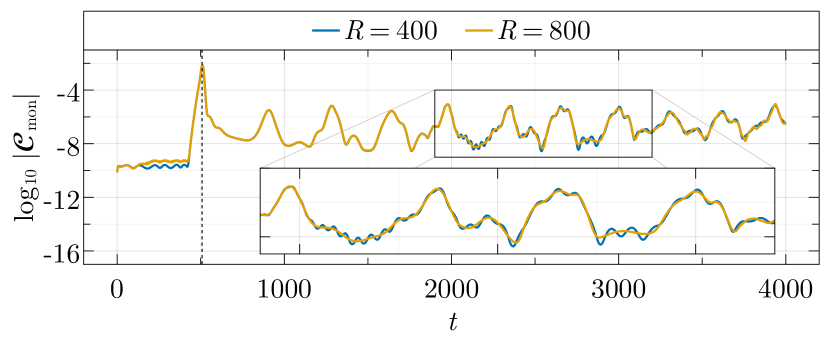
Figure 7: Results from evolution of CTS+CVE data with initial distance $d=80$ and boost parameter $v=0.05$ for polynomial resolution $p=11$ and two differently sized computational domains. Top Comparison of the spatial distribution of scalar-field amplitude $A(t\approx 2000,x)$, domain radius $R=400$ (left) and domain radius $R=800$ (right). Bottom Comparison of the evolution of $\mathcal{C}_{\textrm{mon}}$ for the differently sized computational domains. The vertical dashed line indicates the time of merger as determined by the time of the maximum value of $A_{\textrm{max}}(t)$.

During testing we found that some observables can be polluted with artificial high frequency noise for late times. As an example see $\mathcal{C}_{\textrm{mon}}$ in Fig. 5 for SSP data (top, left) and CVE (top, right) which shows this noise starting to appear at $t\approx 2000$. These artifacts are not physical, but depend on parameters like the initial separation and boost of the stars, and numerical resolution and are caused by the scalar field interacting with the outer boundary conditions, which happens because part of the scalar field is ejected from the central region during and after merger. This hypothesis is confirmed by redoing these simulations with a grid setup where the outer domain boundary is moved from radius $R=400$ to $R=800$. Results of this test are displayed in Fig. 7, which shows the spatial distribution of the scalar-field amplitude $A(t,x)$ (top) extracted at coordinate time $t\approx 2000$ for the two differently sized domains. It is evident that $A(t\approx 2000,x)$ in the smaller domain displays noticeable radial oscillations, whereas they are absent from the scalar-field profile evaluated at the same coordinate time in the larger domain, which reveals these oscillations as artifacts. The comparison of the time evolutions of $\mathcal{C}_{\textrm{mon}}$ (bottom) extracted from these two simulations shows that around $t\approx 2000$ the data is free of noise when the boundary is placed at $R=800$. We note that this strategy of moving the boundary out further and further is in general not a reliable solution when interested in artifact-free long-time evolutions, because the associated computational costs eventually start to become prohibitive. Although it might be possible to mitigate the computational costs by using AMR with properly tuned $hp$ refinement, a more sustainable solution would be to investigate how our boundary conditions need to be adjusted to work with massive complex scalar fields. We leave this task to future work. In the following discussion of global quantities and gravitational waves we show results that were obtained with $R=800$.

V.2 Global quantities

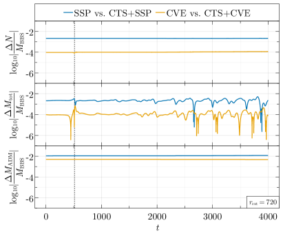
Figure 8: Relative differences of global quantities $N$ (top), $M_{\textrm{tot}}$ (middle), $M_{\textrm{ADM}}$ (bottom) between results from evolutions of SSP data vs. CTS+SSP and evolutions of CVE data vs. CTS+CVE data. The stars were prepared with initial boost parameter $v=0.05$ and initial separation $d=80$ and the differences were computed at polynomial resolution $n=11$. $M_{\textrm{ADM}}$ was extracted at a sphere with coordinate radius $r_{\textrm{ext}}=720$. The vertical dashed line indicates the time of merger as determined by the time of the maximum value of $A_{\textrm{max}}(t)$.

In Fig. 8 we continue the comparison started in Fig. 5 by studying how relative differences in global quantities develop for evolutions that used constraint-violating vs. constraint-satisfying initial data with initial separation $d=80$, boost $v=0.05$ and resolution $n=11$. It is evident from the plot that the relative differences in Noether charge $\Delta N$, ADM mass $\Delta M_{\textrm{ADM}}$ and total mass $\Delta M_{\textrm{tot}}$ are constant in time to a good approximation. The differences between CVE vs. CTS+CVE data evolutions for $\Delta N$ and $\Delta M_{\textrm{tot}}$ are of the order $0.01\%~{}M_{\textrm{BBS}}$, whereas the differences between SSP vs. CTS+SSP evolutions are below $0.1\%~{}M_{\textrm{BBS}}$. The differences in $\Delta M_{\textrm{ADM}}$ are of order $0.1\%~{}M_{\textrm{BBS}}$ and $1\%~{}M_{\textrm{BBS}}$ for CVE vs. CTS+CVE and SSP vs. CTS+SSP, respectively. We want to emphasize that the utilized resolution $n=11$ is rather coarse and computationally inexpensive, but the observed differences are already very small for both data sets.

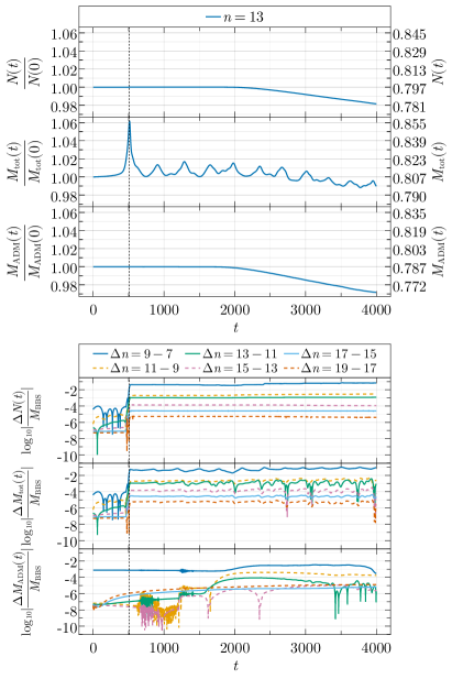
Figure 9: Top Time evolution of the global quantities $N$, $M_{\textrm{tot}}$ and $M_{\textrm{ADM}}$ obtained from a simulation with resolution $n=13$. Bottom Self-convergence test of those variables. Results are from simulations of CTS+CVE data with initial separation $d=80$ and initial boost parameter $v=0.05$. $M_{\textrm{ADM}}$ was extracted at a sphere with coordinate radius $R=720$. The vertical dashed lines indicate the time of merger as determined by the time of the maximum value of $A_{\textrm{max}}(t)$ from the highest resolution.

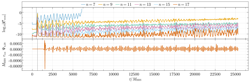
Figure 10: Time evolution of $\mathcal{C}_{\textrm{mon}}$ (top) for simulations based on CTS+CVE data with boost $v=0.05$ and initial separation $d=80$ for different resolutions $n$. Unprocessed $\Psi_{4,20}$ signal (bottom) obtained from the simulation with $n=17$ and extracted on a sphere of radius $r_{\textrm{ext}}=720$. The vertical dashed line indicates the time of merger as determined by the time of the maximum value of $A_{\textrm{max}}(t)$ from the highest resolution.

Fig. 9 displays the time evolutions of $N$, $M_{\textrm{tot}}$ and $M_{\textrm{ADM}}$ (top) as well as a self-convergence study of the same quantities (bottom). These results were obtained from evolutions of runs done with the CTS+CVE data with initial separation $d=80$ and boost parameter $v=0.05$. Focusing first on the upper panel and the top plot which shows $N(t)/N(0)$ one can see that for resolution $n=13$ the relative deviation from the initial value $N(0)$ is well below $1\%$ when $0\leq t\leq 2000$, indicating that $N(t)$ is numerically conserved. On the other hand, for $t\gtrsim 2000$ the Noether charge starts to decrease until $\approx 98\%$ of the initial value is left at $t=4000$. Similar behavior is observed in the evolution of $M_{\textrm{ADM}}(t)/M_{\textrm{ADM}}(0)$, i. e. the ADM mass is conserved well below $1\%$ over the time range $0\leq t\leq 2000$, after which it starts to decrease until it reaches a final value below $97\%$ at $t=4000$. On the other hand, $M_{\textrm{tot}}(t)/M_{\textrm{tot}}(0)$ is by definition not a conserved quantity and this is reflected in its time evolution, because it shows significant oscillations already for $t\leq 2000$. Note also that this quantity shows a decreasing trend for late times. We verified that the apparent loss in $N$, $M_{\textrm{ADM}}$ and $M_{\textrm{tot}}$ is due to the scalar field getting absorbed by the outer boundary conditions, much like the artificial oscillations of $A$ that we discussed in Fig. 7.

Regarding the self-convergence tests displayed in the lower panel, the differences in $\Delta N$ decrease with increasing resolution, confirming that $N$ is indeed convergent. We note that the differences are noticeably increased through the merger, but overall remain roughly constant in time. The differences in $\Delta M_{\textrm{ADM}}$ show more variations in time, but one can still recognize a convergence trend in this data. We attribute this behavioral difference to the fact that $N$ and $M_{\textrm{ADM}}$ are computed through a volume and surface integral, respectively, and the latter being more susceptible to numerical errors, because its computation involves less degrees of freedom than that of a volume integral. The differences in $\Delta M_{\textrm{tot}}$ also behave similarly to $\Delta N$ in the way that they show a convergence pattern, the differences remain roughly constant over time and they are increased through the merger. These plots demonstrate that also global quantities like $\Delta N$ and $\Delta M_{\textrm{tot}}$ converge exponentially.

V.3 Gravitational waves

Fig. 10 shows results of a long-time evolution of a BS head-on with initial separation $d=80$ and initial boost parameter $v=0.05$. The plot shows that the run with the lowest resolution $n=7$ crashed, but starting with $n\geq 9$ a stable convergence pattern can be observed where the exponential improvement between resolutions is maintained also for late times. One can also recognize a growth of $\mathcal{C}_{\textrm{mon}}$ over time, which might become troublesome for even longer evolutions; however, we were able to evolve to at least $t/M_{\textrm{BBS}}=50000$ without problems and there remains the possibility to adjust the GHG damping system through the parameter $\gamma_{0}$ in combination with adjustments to the local grid widths. The $\Psi_{4,20}$ strain extracted from the highest resolved run with $n=17$ displays the characteristic afterglow signature of these kinds of collisions, where the remnant scalar-field cloud is continuing to oscillate and emit gravitational radiation with an amplitude that is of the same order as the merger spike [14]. The dominant amplitude in the frequency spectrum of $\Psi_{4,20}$ is located at

$$f_{\textrm{dom}}\approx 7.7\times 10^{-3}\left(\frac{\mu}{6.582\times 10^{-16}~{}\text{eV}}\right)~{}\text{Hz}\,.$$

Assuming a scalar-field mass $\mu=1\times 10^{-11}~{}\text{eV}$ this translates into $f_{\textrm{dom}}\approx 117~{}\text{Hz}$. Furthemore, the plot shows that the afterglow lasts at least for time

$$T_{\textrm{glow}}\gtrsim 18750\left(\frac{\mu}{6.582\times 10^{-16}~{}\text{eV}}\right)^{-1}~{}\text{s}\,,$$

which corresponds to $T_{\textrm{glow}}\gtrsim 1.2~{}\text{s}$, assuming the same scalar-field mass.

We want to highlight that our computational setup does not involve angular momentum, because the head-on collisions proceed with zero impact parameter and the simulations are carried out in axisymmetry and with reflection symmetry, and yet we do observe a noticable afterglow signature in Fig. 10. Our results therefore demonstrate that the emission of GW afterglow radiation in BS collisions is not solely tied to the presence of angular momentum in the initial data or the remnant.

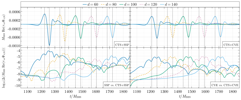
Figure 11: Top $\Psi_{4,20}$ signals obtained from evolutions of CTS+SSP initial data (left) and CTS+CVE initial (right) with polynomial resolution $n=15$, initial boost parameter $v=0.1$ and for varying initial distance $d$. Bottom Differences of $\Psi_{4,20}$ signals between SSP vs. CTS+SSP (left) data and between CVE vs. CTS+CVE data (right). The $\Psi_{4,20}$ data was extracted on a sphere of radius $r_{\textrm{ext}}=720$. The vertical dashed lines indicate the times where the extrema of $\Psi_{4,20}$ appear for each separation $d$.

In [12] a comparison between $\Psi_{4,20}$ signals extracted around the time of merger and obtained from runs using SSP and CVE initial data was already carried out. The binary BS head-on configuration studied in there used the same isolated BS solution as we do for the superposition. The initial boost parameter was fixed to $v=0.1$. In Fig. 11 we reproduce their results for resolution $n=15$, but using instead CTS+SSP initial data (top, left) and CTS+CVE initial data (top, right). Furthermore, we also evolved SSP and CVE initial data and we plot the absolute differences between the $\Psi_{4,20}$ signals obtained from SSP vs. CTS+SSP data (bottom, left) and CVE vs. CTS+CVE data (bottom, right). The data was extracted at spheres with radius $r_{\textrm{ext}}=720$. Focusing on raw $\Psi_{4,20}$ data first (top, left and right), one can observe the same qualitative differences between CTS+SSP and CTS+CVE data that were reported for SSP and CVE data in [12]. The maximum amplitude of $\Psi_{4,20}$ shows a dependence on the initial separation $d$ between the two stars for the runs that used CTS+SSP data, whereas the CTS+CVE results show almost constant maximum amplitude and the wave’s shape is roughly independent of $d$. Furthermore, for $d=80$ the GW signal arrives later by $\Delta t/M_{\textrm{BBS}}\approx 14$ from CTS+SSP data compared to the CTS+CVE data and this time delay decreases to $\Delta t/M_{\textrm{BBS}}\approx 10$ for $d=140$. From the plot showing the differences of $\Psi_{4,20}$, one can read off that the GW signal differs at most by $10^{-4}$ for SSP vs. CTS+SSP data and at most by $10^{-5}$ for CVE vs. CTS+CVE data. When normalized by the maximum amplitude of the $\Psi_{4,20}$ signal, these differences translate into a maximum deviation of $\approx 10\%$ for SSP vs. CTS+SSP and $\approx 2\%$ CVE vs. CTS+CVE data, respectively.

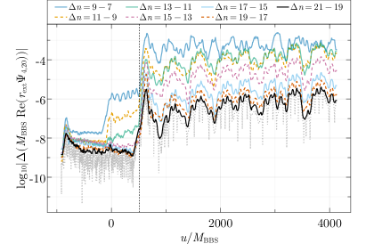
Figure 12: Self-convergence test of $M_{\textrm{BBS}}r_{\textrm{ext}}\Psi_{4,20}$ obtained from evolutions of CVE data with initial separation $d=80$ and boost parameter $v=0.05$. Signals were extracted at coordinate radius $r_{\textrm{ext}}=720$. The solid and dashed lines display differences between two consecutive resolutions of $\Psi_{4,20}$. For visualization purposes the data has been interpolated onto a common time grid for the difference computation and then postprocessed using a moving average filter (see Appendix F). The dotted gray line is the raw difference computed between resolutions $n=19$ and 21, which illustrates that the moving average accurately represents the trend of the data. The vertical dashed line indicates the time of merger as determined by the time of the maximum value of $A_{\textrm{max}}(t)$ from the highest resolution.

Fig. 12 presents a self-convergence test using $\Psi_{4,20}$ signals extracted from evolutions of CTS+CVE initial data with initial separation $d=80$ and boost parameter $v=0.05$. The signals were extracted at spheres with coordinate radius $r_{\textrm{ext}}=720$ and the results are plotted against retarded time $u$. Similar to the self-convergence test of the global quantities $N$, $M_{\textrm{tot}}$ and $M_{\textrm{ADM}}$, one can observe a clear decrease in the differences $\Delta\Psi_{4}$ with increasing polynomial resolution, indicating an exponentially convergent result. The differences increase notably through the merger by roughly two orders of magnitude. The differences between the two highest resolved runs with $n=17$ and $19$ can be interpreted as an error bound on the numerical accuracy of $\Psi_{4,20}$ and we infer that the results are accurate up to $10^{-5}$ for the studied configuration. This bound is conservative, because, as the trend of this convergence test indicates, any differences obtained between two consecutive resolutions that are each higher than $n=19$ will be smaller than this difference.

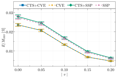
Figure 13: Dependency of the radiated GW energy $E/M_{\textrm{BBS}}$ on the initial boost parameter $v$ obtained from evolutions of SSP, CTS+SSP, CVE and CTS+CVE initial data and fixed initial distance $d=80$ and polynomial resolution $n=15$. The error bars account for finite resolution errors and uncertainties in the postprocessing.

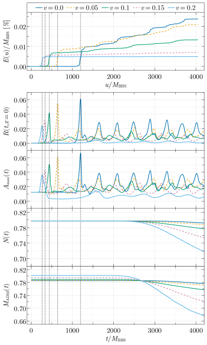
Figure 14: Top Time evolution of $E(u)/M_{\textrm{BBS}}$ vs. retarded time $u/M_{\textrm{BBS}}$ obtained from evolutions of CTS+CVE initial data with fixed initial separation $d=80$ and resolution $n=15$, but varying boost parameter $v$. Bottom Time evolution of $R(t,x=0)$, $A_{\textrm{max}}(t)$, $N(t)$, and $M_{\textrm{ADM}}(t)$ vs. coordinate time $t/M_{\textrm{BBS}}$ from the same simulations. Note that $E/M_{\textrm{BBS}}$ stops growing when $u/M_{\textrm{BBS}}\gtrsim 3800$ for all values of $v$, which is due to the use of a window function in the postprocessing of the data (see App. A for details). The vertical dashed lines indicate the time of merger as determined by the time of the maximum value of $A_{\textrm{max}}(t)$.

In Fig. 13 we compare the radiated gravitational wave energy $E/M_{\textrm{BBS}}$ emitted over a retarded time span of $u\in[100,3000]$ from evolutions of SSP, CTS+SSP, CVE and CTS+CVE initial data, where we fix the initial separation $d=80$ and polynomial resolution $n=15$ and vary the boost parameter $v$. First, the plot shows a difference in $E$ depending on whether SSP or CVE initial data is evolved and this difference decreases with increasing $v$. On the other hand, the difference between $E$ obtained from SSP vs. CTS+SSP and CVE vs. CTS+CVE is comparatively negligible. Taking into account the error bars the conclusion is that one cannot distinguish superposed initial data from constraint-solved data by the amount of radiated energy emitted over this time span. Regarding the dependence on $v$, it is evident that $E$ decreases with increasing $v$. From a physical perspective this is counter intuitive, because increasing $v$ increases the energy of the binary system in the initial slice. Furthermore, with larger $v$ the time to merger is reduced and, thus, there would be more time left for GWs to radiate away from merger till $u=3000$. This behavior is in contrast with a similar experiment that was conducted for BH head-on collisions in [77], where indeed the radiated GW energy increases when increasing $v$. Nevertheless, these results are in accordance with what was observed in [12], where $E$ also decreases when the initial separation $d$ between the stars is increased, which also corresponds to an increase of the total energy in the initial slice.

Analysis of 1D and 2D output from simulations that were used for Fig. 13 shows that with increasing $v$ the gravitational and scalar field both display decreasing amplitudes. To this end, consider Fig. 14 where the time evolution of $E(u)/M_{\textrm{BBS}}$, $R(t,x=0)$, $A_{\textrm{max}}(t)$ $N(t)$ and $M_{\textrm{ADM}}(t)$ is shown for simulations of CTS+CVE data with initial separation $d=80$ and resolution $n=15$, but we vary the boost parameter $v$. First, one can read off the values of $E/M_{\textrm{BBS}}$ at $u/M_{\textrm{BBS}}\approx 4050$ which were shown in Fig. 13 for the CTS+CVE data. The plot displays that the initial burst of radiation is responsible for a significant increase in $E/M_{\textrm{BBS}}(u)$. When contrasted with the evolutions of $R(t,x=0)$ and $A_{\textrm{max}}(t)$, it is apparent that this is caused by the merger where these quantities peak. Furthermore, one observes that with increasing $v$ the first burst is emitted at earlier times, but the strength of the burst also decreases. However, at the same time the flux of $E(u)/M_{\textrm{BBS}}$ radiated in the afterglow phase decreases when $v$ increases. During that phase $R(t,x=0)$ and $A_{\textrm{max}}(t)$ also display a continued decrease in the amplitude of the oscillations. The evolutions of $N(t)$ and $M_{\textrm{ADM}}(t)$ show that until $t/M_{\textrm{BBS}}\approx 2000$ the quantities $N$ and $M_{\textrm{ADM}}$ are both conserved to good approximation. The difference in $M_{\textrm{ADM}}$ when $0\leq t/M_{\textrm{BBS}}\leq 2000$ between different values of $v$ reflects the fact that an increase in the initial momenta of the stars corresponds to initially more energetic configurations. Eventually, both $N(t)$ and $M_{\textrm{ADM}}(t)$ decrease, because the scalar field leaves the computational domain through the boundary. We note that this decrease sets in earlier and proceeds faster when $v=0.2$ than $v=0.0$, which we verified by studying $dN/dt$ (not shown). This allows one to conclude that the larger $v$, the faster energy is carried away through the scalar field being ejected. As a consequence, the produced remnant will be lighter for larger $v$.

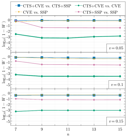
Figure 15: Analysis of the complementary Wiener product $\bar{W}(\Psi_{4,20}^{(1)},\Psi_{4,20}^{(2)})$ between GWs $\Psi_{4,20}^{(1)}$ and $\Psi_{4,20}^{(2)}$ obtained from two initial data sets and for varying numerical resolution $n$. The initial stars were prepared with a separation $d=80$ and boost parameters $v=0.05$ (top), $v=0.1$ (middle), $v=0.15$ (bottom).

Fig. 15 shows the (complementary) Wiener product $\bar{W}:=1-W({\Psi_{4,20}}^{(1)},{\Psi_{4,20}}^{(2)})$ computed between two signals ${\Psi_{4,20}}^{(1)}$ and ${\Psi_{4,20}}^{(2)}$ and obtained from different initial data constructions. The initial distance was fixed to $d=80$, we vary the polynomial resolution $n$ and we show results for boost values $v=$ 0.05, 0.1 and 0.15. We used the T1800044-v5 Advanced LIGO sensitivity design curve [75] to weight the product and the complex scalar field’s mass was fixed to $\mu=1\times 10^{-11}~{}\text{eV}$. $W$ was computed using data that was extrapolated to null infinity with different orders $N_{\textrm{extrp}}$. We remind the reader that a value $\bar{W}=1-W({\Psi_{4,20}}^{(1)},{\Psi_{4,20}}^{(2)})=0$ means that ${\Psi_{4,20}}^{(1)}$ and ${\Psi_{4,20}}^{(2)}$ are identical if they would appear in a detector with the provided noise sensitivity curve. The plot shows, independent of $v$, that $\bar{W}$ is always smallest when comparing $\Psi_{4,20}$ from evolutions of CVE data vs. CTS+CVE data, meaning that these waveforms are the closest to each other among those we compare. The difference between GWs received from SSP data vs. CTS+SSP data is bigger than the one from CVE data vs. CTS+CVE data. $\bar{W}$ is biggest when comparing either SSP data vs. CVE data or CTS+SSP data vs. CTS+CVE data. We note that these qualitative results are to very good agreement independent of the numerical resolution $n$. Furthermore, the results are independent of the extrapolation order $N_{\textrm{extrp}}$, because Fig. 15 already shows the results obtained from analyses where $N_{\textrm{extrp}}$ was varied too, however, the obtained curves all overlap with one another. Overall this picture is consistent with the discussions of other comparisons in this work where it turned out that any apparent differences between analysis quantities are more pronounced when comparing results from SSP data vs. CTS+SSP data than comparing results from CVE data vs. CTS+CVE data.

VI Conclusion

In this manuscript we reported results of long-time stable and accurate binary head-on BS collisions obtained using a PS method as implemented in bamps. We studied variations of a mini BS configuration which was already investigated in [12], but differed in the way the initial data was constructed: two of the data sets (SSP, CVE) were obtained from a superposition of isolated stars and thus carried initial constraint violations, whereas the other two data sets (CTS+SSP, CTS+CVE) were obtained by numerically solving the CTS equations and with free data based on SSP and CVE data, using the hyperbolic relaxation method presented in [47]. In our work we did not enforce quasi-equilibrium conditions to ease our comparison with previous work in [12]. This effort was undertaken to answer the question of how much of a difference one can expect physical observables to vary when numerically evolving constraint-violating and satisfying data.

In summary we found that the differences in the discussed analysis quantities computed during evolutions, among which is also the constraint monitor of bamps, are always bigger between SSP vs. CTS+SSP data when compared to CVE vs. CTS+CVE data. We demonstrated that evolutions of SSP and CVE data bear residual constraint violations above $10^{-8}$ and $10^{-10}$, respectively, despite being self-convergent. On the other hand, we could reduce and preserve the constraint violations for CTS+SSP and CTS+CVE data well below $10^{-10}$ using a reasonable resolution, which demonstrates the capabilities of PS approximations as viable methods for next generation NR codes targeted at smooth solutions. A study of global analysis quantities showed that conserved variables like Noether charge $N$ and ADM mass $M_{\textrm{ADM}}$ can be preserved well below $1\%$ of their initial value already starting with comparatively small polynomial order $n=9$ per grid, as long as the scalar field does not leave the computational domain, while at the same time also displaying exponential decrease in a self-convergence study.

A direct comparison of the Ricci scalar at the collision center $R(x=0)$ and the scalar field amplitude $A_{\textrm{max}}$ between results obtained from SSP vs. CTS+SSP showed that these quantities eventually start to dephase after merger. No such deviations were observed when comparing results from evolutions of CVE vs. CTS+CVE initial data. The main motivation for the development of the CVE method in [12] was that for head-on collisions of solitonic BSs $A_{\textrm{max}}$ obtained from SSP data displayed an artificial growth during the infall phase and eventually lead to premature BH collapse. This growth was avoided by the use of the CVE construction, which also delayed the BH formation after the stars’ centers merged. Although, this work was concerned with mini BS collisions for which no BH collapse occurs, we find a qualitatively similar behavior for $A_{\textrm{max}}$ when evolving SSP and CVE data. Furthermore, the constraint-solved CTS+SSP data did not cure this artificial growth pre-merger. On the other hand, the evolution of $A_{\textrm{max}}$ obtained from CTS+CVE data is to good approximation identical to the CVE data, i. e. $A_{\textrm{max}}$ remains approximately constant during infall when the centers of the stars are well separated. This latter observation serves as an argument which favors the use of CVE and CTS+CVE data over SSP and CTS+SSP data, in particular, when the goal is to model the coalescence of initially non-interacting stars that fall in on each other.

We reproduced the $\Psi_{4,20}$ signals of the mini BS head-on collisions that were reported in [12] for SSP and CVE data and compared these findings with signals obtained from CTS+SSP and CTS+CVE data. We found that constraint solving does not significantly alter the qualitative differences that were discussed in [12]. These results are robust, as we demonstrated exponential decrease in differences of $\Psi_{4,20}$ signals in a self-convergence study. We then computed the radiated energy from these kinds of head-on collisions while also varying the initial boost parameter $v$ and found, again, a difference that is dominated by the way in which the isolated stars are superposed. For this quantity differences due to constraint solving the initial data are negligible and indistinguishable when accounting for errors in postprocessing. The analysis of the errors required special attention due to the lack of a heuristic cutoff frequency for signals originating from head-on collisions and which is used to suppress nonlinear drifts in the GW reconstruction (see App. A).

An interesting physical result is that the radiated energy emitted during a fixed interval of coordinate time decreases when the initial momenta of the stars is increased, which is in opposition to BH head-on collisions where increasing the progenitors initial momenta leads to more energy being radiated gravitationally [77]. However, these findings are conceptually in agreement with results presented in [12] where for fixed boost parameter $v$ the radiated energy also decreases when the initial distance between two BSs is increased, which also corresponds to an increase of the total energy of the system. This qualitative behavior is independent of the quality of the initial data, but quantitative differences in total radiated energy could be observed.

We quantified the difference in the shape of the GW signals by computing the Wiener product between results of SSP, CVE, CTS+SSP and CTS+CVE initial data and varying resolutions, while taking into account detector noise. Here we found that signals obtained from CVE vs. CTS+CVE data are more similar to one another than signals obtained from SSP vs. CTS+SSP data. Comparing signals between SSP vs. CVE and CTS+SSP vs. CTS+CVE showed that the way in which the superposition of stars is done dominates any effects due to constraint violations, which is in agreement with the rest of our findings.

Overall we can conclude that all the differences we observed in the analysis quantities we studied, and for the particular BS head-on configuration we considered, are dominated by the way in which the SSP and CVE constructions differ. Differences in physical observables due to constraint violations were comparatively negligible, and marginally relevant when accounting for errors. This result is reassuring for theoretical predictions that were made based on BS simulations that used superposed data and for which it was verified that the initial constraint violations were reasonably small. Nevertheless, we recommend the use of constraint-satisfying over constraint-violating initial data for multiple reasons. First, solutions to the EFEs satisfy the constraint equations exactly at all times, which includes the initial slice, and, thus, the goal for numerical approximations of these solutions should be to satisfy these equations as well as possible. In practice it is also easier to preserve small initial constraint violations in time than having to rely on large initial constraint violations being reduced in time through a damping scheme, or having to rely on them to leave the computational domain through a boundary. Furthermore, it is not uncommon in long-time evolutions to find that constraint violations eventually start to grow for late times. In such a scenario, constraint-satisfying data will likely allow to evolve for longer times than constraint-violating data would, because the former leaves more room for the growth of violations during the evolution until the result becomes dominated by errors or the simulation crashes.

This work established the basis for future studies of BS evolutions with the bamps code. With the addition of AMR support in bamps [48] and the nice convergence behavior demonstrated in this work, we are confident that our code will be able to perform high-resolution and long-time-stable simulations of binary inspiraling BS collisions to produce quality GW signals. A future goal is to eventually build a waveform template bank for a targeted search of merger signals involving exotic compact objects. Another avenue worth exploring would be the problem of the construction of quasi-equilibrium initial data for which first work has started in [25]. In particular the hyperbolic relaxation method used to solve the CTS equations in the present paper is directly implemented in bamps and, as such, it can profit from all optimizations that are added to the evolution code, which should enable generation of high quality initial data with a moderate amount of computational resources.

Appendix A Gravitational wave analysis

Below we outline the GW analysis used in bamps and describe the postprocessing techniques used for the analysis of the data presented in the main text.

The bamps code employs the Newman-Penrose formalism [85] to compute the curvature pseudo-scalar field $\Psi_{4}$, which measures radially outgoing gravitational radiation. The actual implementation follows the standard procedure outlined in [86] (see also [87] for a review), where $\Psi_{4}$ is first computed from the Weyl tensor and an orthonormal null tetrad, which itself is constructed from an orthonormal basis adapted to the normal direction of spheres centered around the collision region. Taking into account the pseudo-scalar characteristic of $\Psi_{4}$, it is then decomposed into a modal expansion of spin-weighted spherical harmonics ${}_{-2}Y_{lm}$ with complex coefficients $\Psi_{4,lm}$, where $l\geq 2,m=-l,\dots,l$.

For the analysis of head-on collisions, which take place in axisymmetry, only the expansion coefficients with $l$ even and $m=0$ are non-zero, and are purely real [77]. In this work we only analyze the dominant $l,m=2,0$ mode.

The GW flux and strain is reconstructed from [86]

$$\frac{\differential rh_{20}}{\differential t}(t) =\lim_{r\to\infty}\int^{t}_{-\infty}\differential t^{\prime}~{}r\Psi_{4,20}(t^{\prime},r)\,,$$ (42)

$$rh_{20}(t) =\lim_{r\to\infty}\int^{t}_{-\infty}\differential t^{\prime}\int_{-\infty}^{t^{\prime}}\differential t^{\prime\prime}~{}r\Psi_{4,20}(t^{\prime\prime},r)\,,$$ (43)

and the radiated energy associated with $\Psi_{4,20}$ is computed from

$$E(t) =\int^{t}_{-\infty}\differential t^{\prime}~{}\frac{\differential E(t^{\prime})}{\differential t}\,,$$ (44)

$$\frac{\differential E}{\differential t}(t) =\lim_{r\to\infty}\frac{1}{16\pi}\left|\int^{t}_{-\infty}\differential t^{\prime}~{}r\Psi_{4,20}(t^{\prime},r)\right|^{2}\,.$$ (45)

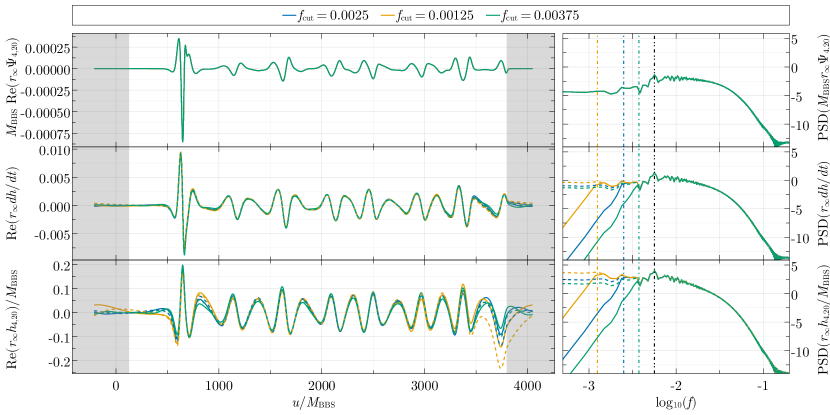
Figure 16: $r_{\infty}\Psi_{4,20}$ (top) signal and its PSD extrapolated to null infinity with $N_{\textrm{extrp}}=3$ and data obtained from a simulation of CTS+CVE initial data with polynomial resolution $n=15$, initial separation $d=80$ and boost parameter $v=0.05$. Gray shaded areas indicate where the windowing (49) was applied. $dh/dt$ (middle) and $h$ (bottom) are results obtained with the methods discussed in the text: modified FFI method (solid, with extra Butterworth high-pass filtering), standard FFI method (dashed). Vertically dashed-dotted lines correspond to the different cutoff frequencies used and vertically dash-double-dotted lines correspond to the frequency of the maximum amplitude in $\text{PSD}(M_{\textrm{BBS}}r_{\textrm{ext}}\Psi_{4,20})$.

In order to carry out the limit $r\to\infty$ above we utilize the peeling property of $\Psi_{4}$ [85] and perform an extrapolation in radius $r$ before integration. To this end, we introduce the retarded time coordinate

$$u(t) =u_{\ast}(t)-t_{\ast}\,,$$

$$=t-r-2M_{\textrm{BBS}}\log\left(\frac{r}{2M_{\textrm{BBS}}}-1\right)-t_{\ast}\,,$$ (46)

where $t_{\ast}$ is a constant that is added in order to correct the retarded Schwarzschild time coordinate $u_{\ast}$ to account for a potential time dependence of the lapse and the radial coordinate in the far field zone, as well as for the fact that the $r$ used in our simulations is in general not an areal coordinate in our gauge [88]. $t_{\ast}$ is determined numerically by aligning multiple $\Psi_{4,20}$ data streams extracted at different radii $r_{\textrm{ext}}$ at the first zero before the merger spike. We note that in [88, 89] more sophisticated expressions for determining $t_{\ast}$ were provided which can also account for departures of the standard tortoise Schwarzschild coordinate. Their method requires extra simulation output, but we found that numerically determining $t_{\ast}$ in a postprocessing step can also improve the quality of the extrapolation to null infinity to a satisfying degree, as we discuss next.

The so obtained time aligned $\Psi_{4,20}$ data streams recorded at $N$ different extraction radii ${r_{\textrm{ext}}}_{,1}\leq\dots\leq{r_{\textrm{ext}}}_{,N}$ are then fitted to the ansatz

$$r\Psi_{4,20}(u)=r_{\infty}\Psi_{4,20}(u)+\sum_{n=1}^{N_{\textrm{extrp}}}\frac{\alpha_{n}(u)}{r^{n}}\,,$$ (47)

using the linear least squares method to determine the time dependent coefficients $r_{\infty}\Psi_{4,20}$ and $\alpha_{n}$. The desired extrapolated curvature scalar for the evaluation of (42), (43) and (45) is then given by $r_{\infty}\Psi_{4,20}$. We note that the quality of the extrapolated result depends 1) on the number and range of extraction radii ${r_{\textrm{ext}}}_{,N}-{r_{\textrm{ext}}}_{,1}$ on which data is recorded (the more, the better), 2) the extrapolation order $N_{\textrm{extrp}}$, and 3) the time alignment through the correction $t_{\ast}$. All results involving $\Psi_{4,20}$ and presented in this work were obtained from simulations where the outermost boundary was located at $R=800$ and we recorded $\Psi_{4,20}$ data on 48 spheres with equally spaced increments between ${r_{\textrm{ext}}}_{,1}=200$ and ${r_{\textrm{ext}}}_{,N}=800$. The extrapolations to null infinity of $r_{\infty}\Psi_{4,20}$ were only used for Fig. 13, Fig. 14 and Fig. 15, for which we verified that the results are stable between extrapolations that used different orders $N_{\textrm{extrp}}=1,\dots,5$.

The last ingredient for the analysis is the numerical evaluation of time integrals appearing in the reconstruction formulae. To this end we first preprocess the $r_{\infty}\Psi_{4,20}$ data by limiting it to a range $u\in[u_{L},u_{R}]$ with

$$w(u,\bar{u},\sigma) =\frac{1}{2}(\tanh(\sigma(u-\bar{u}))-1)\,,$$ (48)

$$r_{\infty}\Psi_{4,20}^{\prime}(u) =r_{\infty}\Psi_{4,20}(u)$$

$$\times w(u,u_{L},\sigma)w(u,u_{R},-\sigma)\,.$$ (49)

We used $\sigma=1/10$, $u_{L}=100$ and $u_{R}=3000$ for all our analysis to make the signal periodic in $u$, which avoids additional artifacts when Fourier analyzing the signal later on. We note that the choice of $u_{L}$ is such that the dominant spike in the analysis of all studied GW signals is not affected by the windowing, even when the boost parameter is $v=0.2$. Given the windowed data, we then evaluate the integrals using a variation of the fixed frequency method (FFI) [90], which requires a choice for the cutoff frequency $f_{\textrm{cut}}$ to remove spurious nonlinear drifts and we comment on this further below. In our variation to the FFI method we first apply a discrete Fourier transform (DFT) to the windowed data to obtain $\mathcal{F}(r_{\infty}\Psi_{4,20})$, we then apply a high-pass Butterworth filter of order $N=10$ with transfer function $H_{N}(f,f_{\textrm{cut}})$ to obtain

$$\mathcal{F^{\prime}}(r_{\infty}\Psi_{4,20})=\mathcal{F}(r_{\infty}\Psi_{4,20})|H_{N}(f,f_{\textrm{cut}})|\,,$$ (50)

and finally perform the FFI integration with $\mathcal{F^{\prime}}(r_{\infty}\Psi_{4,20})$ and cutoff $f_{\textrm{cut}}$ to compute (42), (43) and (45). Lastly, to compute $E$ via (44) we resort to using a standard trapezoidal rule, since $E(t)$ will be monotonically increasing and the FFI method can only be used for oscillating signals.

Fig. 16 shows an example of an extrapolated and windowed $\Psi_{4,20}$ data stream, reconstructions $\differential h_{4,20}/\differential t$ and $h_{4,20}$, as well as the respective power spectral densities (PSDs), that were computed with three different values for $f_{\textrm{cut}}$ (see legend). The PSD of the $\differential h_{4,20}/\differential t$ results show that the integration amplified small frequency components and the additional processing via a Butterworth high-pass filter exponentially suppresses this growth for frequencies below $f_{\textrm{cut}}$. The choice of $f_{\textrm{cut}}$ appears to have a mild impact on the time domain signal $\differential h_{4,20}/\differential t$. On the other hand, the PSD of $h_{4,20}$ demonstrates that for too small values of $f_{\textrm{cut}}$ low frequency components are amplified to a level that they become comparable to components above $f_{\textrm{cut}}$. This translates into a strong dependence of the time domain signal on the choice of $f_{\textrm{cut}}$, even when using the Butterworth filter. From this test we conclude that $\differential h_{4,20}/\differential t$ is robust enough for the computations of $\differential E/\differential t$ and $E$ via (45) and (44), whereas the quality of $h_{4,20}$ in our analysis is not sufficient for further studies and we leave it to future work to improve on this.

In [90] it was established that a good choice for the cutoff frequency for the $(l,m)=(2,2)$ mode for binary inspiral simulations is given by $f_{\textrm{cut}}\approx 2f_{\textrm{orb}}$, where $f_{\textrm{orb}}$ is the initial orbital frequency of the stars. Unfortunately, we are not aware of a similar heuristic for head-ons due to the absence of orbital motion and the time domain signal displaying a dominant pulse due to the merger. The three values of $f_{\textrm{cut}}$ given in Fig. 16 are used for all computations of $E$ for which results are shown in the main text (including varying the boost parameter). The associated error bars account for 1) finite resolution errors and 2) uncertainties due to variation in the extrapolation order $N_{\textrm{extrp}}$ and variation in $f_{\textrm{cut}}$. To estimate those contributions we proceed as follows. We compute $E$ for two resolutions $n=13$ and $n=15$ and for all combinations of $N_{\textrm{extrp}}$ and $f_{\textrm{cut}}$. The contribution 1) is taken to be the maximum of all differences of $E$ between results of resolution $n=13$ and $n=15$, but the same values of $N_{\textrm{extrp}}$ and $f_{\textrm{cut}}$. For contribution 2) we compute the average of all $E$ results obtained for $n=15$ and all combinations of $N_{\textrm{extrp}}$ and $f_{\textrm{cut}}$. The associated error is then defined as the maximum of all differences of $E$ and the average of $E$. These two errors are then combined in quadrature and added in Fig. 13. We note that the finite resolution error is on average two orders of magnitude smaller than the error due to the uncertainties involved in the postprocessing.

Appendix B Comparison of waveforms

For GW analysis and parameter estimation studies one often assumes Gaussian noise distribution, which motivates the definition of a detector-noise-weighted inner product (Wiener product) [91, 92] to study the space of real time signals $a(t)$ and $b(t)$. It is defined as

$$(a|b)_{S_{n},[0,\infty)}=\int_{0}^{\infty}\differential f~{}\frac{\tilde{a}(f){\tilde{b}}^{\ast}(f)}{S_{n}(f)}\,,$$ (51)

where $\tilde{a}(f)$ and $\tilde{b}(f)$ are the respective Fourier transforms and $S_{n}(f)$ is the PSD of the noise $n(t)$. This product defines a norm which is positive-definite and assigns an Euclidean structure to the vector space of real signals [91]. If one is given two normalized signals $\hat{a}$ and $\hat{b}$, such that $(\hat{a},\hat{a})_{S_{n},[0,\infty)}=1$ and analogously for $\hat{b}$, then a result of $(\hat{a},\hat{b})_{S_{n},[0,\infty)}$ that is close to 1 indicates that $a$ and $b$ are close to each other.

In practice, one often utilizes the GW strain $h$ together with (51) for parameter studies. However, the reconstruction of $h$ from $\Psi_{4}$ can suffer from uncertainties and even render an analysis based on $h$ useless. Recently, in the context of Proca star head-on collision it was shown in [79] that an analysis using $\Psi_{4}$ data together with (51) and second differenced Gaussian noise PSD $S_{\Psi_{4}}$ is equivalent to the more commonly practiced analysis based on $h$ and $S_{n}$, while at the same time it removes the uncertainties due to free parameters in the $h$ reconstruction procedure. For the results presented in the main text we adopted this analysis which requires additional (but parameter free) processing. In particular, given two $\Psi_{4,20}(u)$ data streams we compute [79] (in practice we use the extrapolated $r_{\infty}\Psi_{4,20}$ data)

$$\tilde{\Psi}^{\prime}_{4,20}[k] =\frac{1-\cos(2\pi k\Delta f\Delta t)}{2\pi^{2}(k\Delta f\Delta t)^{2}}\tilde{\Psi}_{4,20}(k\Delta f)\,,$$ (52)

$$k =0,\dots,N_{d}-1\,,$$

where $\tilde{\Psi}_{4,20}(f)$ is the DFT of $\Psi_{4,20}$, $N_{d}$ is the length of the output data stream, $\Delta t$ is the time resolution of $\Psi_{4,20}$ and $\Delta f=1/(N_{d}\Delta t)$. This transformation relates the second differenced Fourier transform $\tilde{\Psi}^{\prime}_{4,20}$ with the Fourier transform of the second derivative $\tilde{\Psi}_{4,20}=\tilde{\ddot{h}}$. In this work we exclusively used the T1800044-v5 Advanced LIGO sensitivity design curve [75] for $S_{n}$ which is also processed through [79]

$$S_{\Psi_{4}}[k]=\frac{1}{(\Delta t)^{4}} \left(6-8\cos(\frac{2\pi k}{N_{d}})+\right.$$

$$\left.+2\cos(\frac{4\pi k}{N_{d}})\right)S_{n}[k]\,.$$ (53)

Given these quantities we then compute the Wiener product between two signals $\Psi^{(1)}_{4,20}$ and $\Psi^{(2)}_{4,20}$ by

$$W(\Psi^{(1)}_{4,20},\Psi^{(2)}_{4,20}):=(\hat{\Psi}^{(1)}_{4,20}|\hat{\Psi}^{(2)}_{4,20})_{S_{\Psi_{4}},[f_{\textrm{min}},f_{\textrm{max}}]}\,,$$ (54)

where we limited the integration to the range $[f_{\textrm{min}},f_{\textrm{max}}]=[5~{}\text{Hz},1000~{}\text{Hz}]$ for practical purposes, since the detector PSD is only sampled for a finite frequency range. The numerical evaluation of the integral is carried out by using a cubic interpolation to map $\tilde{\Psi}_{4,1}$, $\tilde{\Psi}_{4,2}$ and $S_{\Psi_{4}}$ to a common frequency grid and then use a trapezoidal quadrature rule to compute the integral in (51). We verified that the results presented in Fig. 15 are insensitive to the choice of frequency range. We want to point out that care must be taken when evaluating  (52) and (53), since a limited frequency range $[f_{\textrm{min}},f_{\textrm{max}}]$ also limits the range of $k$ indices to use for numerical integration, because $f_{k}=k\Delta f$.

The results in the main text are presented in Planck units and with a particular choice of rescaling of all quantities (see App. C). Because of that, the obtained results depend on the experimentally unknown scalar-field mass $\mu$. The choice of $\mu$ influences e. g. the time scale with which physical processes take place and, thus, controls the frequency of the GW signals when converted to SI units. Since we are only interested in directly comparing GWs obtained from different initial data construction techniques, we decided to fix $\mu=1~{}\times~{}10^{-11}~{}\text{eV}$ for all computations. With this choice the GW’s spectrum falls roughly into the sensitive region of the detector for the range of boost parameters $v$ we study, i. e. the frequencies of the dominant amplitudes of the PSD of $\Psi_{4,20}$ are then $\mathcal{O}(100~{}\text{Hz})$ [76].

Appendix C Unit systems

Let $l$, $t$, $m$ and $A$ denote length, time, mass and scalar-field amplitude and let $\hat{l}$, $\hat{t}$, $\hat{m}$ and $\hat{A}$ be the numerical values given with respect to reference values $l_{0}$, $t_{0}$, $m_{0}$ and $A_{0}$, i. e.

$$l =\hat{l}~{}l_{0}\,, t =\hat{t}~{}t_{0}\,, m =\hat{m}~{}m_{0}\,, A =\hat{A}~{}A_{0}\,.$$ (55)

In the main text we use the Planck unit system in which $G=c=\hbar=1$. From the definition of the Planck length, time, and mass

$$L_{\textrm{Pl}} =\sqrt{\frac{\hbar G}{c^{3}}}\,, T_{\textrm{Pl}} =\sqrt{\frac{\hbar G}{c^{5}}}\,, M_{\textrm{Pl}} =\sqrt{\frac{\hbar c}{G}}\,,$$ (56)

respectively, we then infer that $L_{\textrm{Pl}}=T_{\textrm{Pl}}=M_{\textrm{Pl}}=1$ holds in such a system. Furthermore, all quantities effectively lose their physical dimensions and $l_{0}$, $t_{0}$, $m_{0}$ and $A_{0}$ now merely serve as dimensionless rescalings. One possible choice for reference values in which this is realized is

$$l_{0} =1/\mu\,, t_{0} =1/\mu\,, A_{0} =1\,,$$ (57)

where $\mu$ is the scalar-field mass introduced in the main text, and we fix $m_{0}$ further below. The numerical values of Planck length and time then read $\hat{L}_{\textrm{Pl}}=\hat{T}_{\textrm{Pl}}=\mu$. This is a convenient choice, because it eliminates $\mu$ from all equations without loss of generality. To see this consider the action (1), which is the fundamental object of the theory under study. Using (57) we can rewrite it as

$$S =\hat{S}S_{0}=\frac{1}{\mu^{2}}\int\differential^{4}\hat{x}\sqrt{-g}$$ (58)

$$\times\left(\frac{\tensor{[}^{(4)}]{\hat{R}}{}}{16\pi}-\frac{1}{2}\left(g^{ab}\hat{\nabla}_{a}\hat{\phi}^{\ast}\hat{\nabla}_{b}\hat{\phi}+|\hat{\phi}|^{2}\right)\right)\,,$$

where we omit carets from $\sqrt{-g}$ and $g^{ab}$, since they are rescaled together with $\differential^{4}x$ and $(\nabla_{a}\cdot)(\nabla_{b}\cdot)$, respectively. Choosing $S_{0}=1/\mu^{2}$ as the reference value for the action then eliminates all factors of $\mu$, such that (58) is formally equivalent to (1) when also setting $\mu=1$ in (5), which was done in the main text.

We note that $m_{0}$ need not be specified in order to obtain (58). Instead, one way to fix it is by demanding

$$1=\hat{\hbar}S_{0}=\hbar=\frac{M_{\textrm{Pl}}L_{\textrm{Pl}}^{2}}{T_{\textrm{Pl}}}=\frac{\hat{M}_{\textrm{Pl}}\hat{L}_{\textrm{Pl}}^{2}}{\hat{T}_{\textrm{Pl}}}\frac{m_{0}l_{0}^{2}}{t_{0}}\,,$$ (59)

so that

$$\hat{\hbar} =\hat{M}_{\textrm{Pl}}\mu\,, S_{0} =\frac{1}{\mu^{2}}=\frac{m_{0}l_{0}^{2}}{t_{0}}\,,$$ (60)

which implies

$$m_{0} =1/\mu\,.$$ (61)

In summary, (57) and (61) are the reference values one can adopt to eliminate all occurrences of $\mu$ from all equations when working with Planck units and BSs.

Another set of units commonly found in the literature are the natural units in which $\hbar=c=1$. From (56) one then obtains the relations $L_{\textrm{Pl}}=T_{\textrm{Pl}}=1/M_{\textrm{Pl}}$ and the Einstein-Hilbert term in the action also attains an extra factor of $1/G=M_{\textrm{Pl}}^{2}$. Thus, when working in such units we recommend the choice

$$l_{0} =1/\mu\,, t_{0} =1/\mu\,, A_{0} =M_{\textrm{Pl}}\,,$$ (62)

as reference values. This then allows to adopt $S_{0}=M_{\textrm{Pl}}^{2}/\mu^{2}$ as the reference value for the action so that all occurrences of $\mu$ and $M_{\textrm{Pl}}$ are eliminated from it. Again, to arrive at $S_{0}$ we need not specify $m_{0}$. Instead the latter is fixed by a similar argument as used for (59) and (60), which yields

$$m_{0} =\frac{M_{\textrm{Pl}}^{2}}{\mu}\,.$$ (63)

In summary, (62) and (63) are a convenient choice of reference values one can adopt when working with natural units and BSs to eliminate all factors of $\mu$ and $M_{\textrm{Pl}}$ from the equations.

We note that [12, 93] also works with natural units but uses

$$l_{0} =1/\mu\,, t_{0} =1/\mu\,, m_{0} =1/\mu\,, A_{0} =M_{\textrm{Pl}}\,.$$ (64)

This set of reference values also removes all factors of $\mu$ and $M_{\textrm{Pl}}$ from the action. However, we find that this choice is not compatible with other parts of our analysis. As an example consider the $g_{rr}$ component in  (69) which, when expressed in natural units and non-rescaled variables, must read

$$\frac{1}{g_{rr}}=1-\frac{2Gm}{r}=1-\frac{2m}{M_{\textrm{Pl}}^{2}r}\,,$$ (65)

since $g_{rr}$ is dimensionless. Performing a rescaling using our convention (62) and (63) eliminates $M_{\textrm{Pl}}$, whereas using (64) does not.

Yet another set of units that is commonly used are geometric units in which $G=c=1$. From (56) one obtains $L_{\textrm{Pl}}=T_{\textrm{Pl}}=M_{\textrm{Pl}}$ and now only the term involving the scalar-field potential in the action attains an extra factor of $1/\hbar^{2}=1/M_{\textrm{Pl}}^{4}$. For this setup we recommend the choice

$$l_{0} =M_{\textrm{Pl}}^{2}/\mu\,, l_{0} =M_{\textrm{Pl}}^{2}/\mu\,, A_{0} =1\,.$$ (66)

This then allows to adopt $S_{0}=M_{\textrm{Pl}}^{4}/\mu^{2}$ to eliminate all factors of $\mu$ and $M_{\textrm{Pl}}$ from the action. By a similar argument we used before, we fix now $m_{0}$ through

$$M_{\textrm{Pl}}^{2}=\hbar=\hat{\hbar}S_{0}=\hat{\hbar}\frac{m_{0}l_{0}^{2}}{t_{0}}\,,$$ (67)

and find

$$m_{0}=M_{\textrm{Pl}}^{2}/\mu\,.$$ (68)

In summary, (66) and (68) are a convenient choice of reference values one can adopt when working with geometric units and BSs to eliminate all factors of $\mu$ and $M_{\textrm{Pl}}$ from the equations.

Appendix D Construction of isolated boson stars in 1D

In this appendix we fix a typo from [12] in the equations that describe stationary, spherically symmetric and isolated BS models. The starting point for the construction of such stars are ansätze for the metric and scalar field which are of the form

$$\differential s^{2} =-e^{2\Phi}\differential t^{2}+\left(1-\frac{2m}{r}\right)^{-1}\differential r^{2}$$

$$+r^{2}\left(\differential\theta^{2}+\sin(\theta)^{2}\differential\varphi^{2}\right)\,,$$ (69)

$$\phi(t,r) =A(r)e^{i\omega t}\,,$$ (70)

where $A,\omega$ are the amplitude and harmonic angular frequency of the scalar field. Inserting these into the EKG system yields

$$\partial_{r}\Phi =\frac{m}{r(r-2m)}$$

$$+\frac{2\pi r^{2}}{r-2m}\left(\eta^{2}+\omega^{2}e^{-2\Phi}A^{2}-V\right)\,,$$ (71)

$$\partial_{r}m =2\pi r^{2}\left(\eta^{2}+\omega^{2}e^{-2\Phi}A^{2}+V\right)\,,$$ (72)

$$\partial_{r}A =\left(1-\frac{2m}{r}\right)^{-1/2}\eta\,,$$ (73)

$$\partial_{r}\eta =-2\frac{\eta}{r}-\eta\partial_{r}\Phi$$

$$+\left(1-\frac{2m}{r}\right)^{-1/2}\left(V^{\prime}-\omega^{2}e^{-2\Phi}\right)A\,,$$ (74)

where $V^{\prime}=\differential V/\differential A^{2}$. In [12] a factor $r/(r-2m)$ was missing in the second term on the RHS in (71).

This system of equation is subjected to the boundary conditions

$$A(0) =A_{\textrm{ctr}}\,, m(0) =0\,, \eta(0) =0\,,$$ (75)

$$\partial_{r}\Phi(0) =0\,, \lim_{r\to\infty}A(r) \to 0\,.$$ (76)

The asymptotic behavior of $A$ is given by

$$A\sim\frac{1}{r^{1+\epsilon}}e^{-r\sqrt{1-\omega^{2}e^{-2\Phi}}}\,,$$ (77)

where $\epsilon$ is a non-integer correction that was already reported in [10] and recently discussed in [93].

Our numerical implementation uses the same shooting algorithm as [12], where integration starts at $r=0$ and proceeds radially outwards. The asymptotic behavior is used for patching the solution at a radius $r_{m}$, determined dynamically during integration, beyond which the scalar field is no longer integrated, but instead frozen to the behavior (77). Results presented in this work do not account for the $\epsilon$ correction, as we were simply not aware of it when doing the analysis. However, we implemented the correction in hindsight and found that our single star solutions are only altered in $A$ and $\eta$ in the far-field regime by $\mathcal{O}(10^{-10})$, which is negligible when compared to other error sources.

Appendix E Conformal metric and its time derivative

We note a difference in notation between [71] and our work which is mainly based on [52]. In particular, [52] defines the time derivative of the conformal metric $\bar{\gamma}_{ij}$ as

$$\bar{u}_{ij}:=\partial_{t}\bar{\gamma}_{ij}=-\bar{\gamma}_{ik}\bar{\gamma}_{jl}\partial_{t}\bar{\gamma}^{kl}\,.$$ (78)

Its indices are also raised with the conformal metric,

$$\bar{u}^{mn}=\bar{\gamma}^{im}\bar{\gamma}^{jn}\bar{u}_{ij}\,.$$ (79)

Using (78) we obtain

$$\bar{u}^{mn}=-\partial_{t}\bar{\gamma}^{mn}\,.$$ (80)

On the other hand, [71] does not work with (80), but instead uses

$$\dot{\bar{\gamma}}_{ij} :=\partial_{t}\bar{\gamma}_{ij}\,, \dot{\bar{\gamma}}^{ij} :=\partial_{t}\bar{\gamma}^{ij}\,.$$ (81)

To make the connection with their notation we had to set $\bar{u}^{mn}=-\dot{\bar{\gamma}}^{mn}$, which explains the change in sign in (31).

Appendix F Moving average

The differences between $\Psi_{4,20}$ obtained from different resolutions $n$ are postprocessed for the purpose of demonstrating self-convergence in Fig. 12. To this end, the data is interpolated to a common time grid using cubic splines and $N=2000$ points, after which differences between consecutive resolutions are computed. To suppress the artificial noise due to zero crossings introduced by interpolation errors, and which are amplified on a logarithmic scale, we apply a moving average filter to these differences. In particular, let $\Delta\Psi_{4,i},i=1,\dots,N$ be the difference between two interpolated data streams and let $w$ be an averaging window width, assumed to be even and positive. We define the moving average as

$$\text{avg}[\Delta\Psi_{4,i}] =\frac{1}{w}\sum_{j=1}^{w}\Delta\Psi_{4,i-w/2+j}\,, i \in\left[1+\frac{w}{2},N-\frac{w}{2}\right]\,,$$

$$\text{avg}[\Delta\Psi_{4,i}] =\text{avg}[\Delta\Psi_{4,w/2}]\,, i \in\left[1,\dots,\frac{w}{2}\right]\,,$$

$$\text{avg}[\Delta\Psi_{4,i}] =\text{avg}[\Delta\Psi_{4,N-w/2}]\,, i \in\left[N-\frac{w}{2}+1,N\right]\,.$$

For the data presented in this work we chose $w=20$.

References

- Pretorius [2005] F. Pretorius, Evolution of binary black hole spacetimes, Phys. Rev. Lett. 95, 121101 (2005), arXiv:gr-qc/0507014 .
- Campanelli et al. [2006] M. Campanelli, C. O. Lousto, P. Marronetti, and Y. Zlochower, Accurate evolutions of orbiting black-hole binaries without excision, Phys. Rev. Lett. 96, 111101 (2006), arXiv:gr-qc/0511048 .
- Baker et al. [2006] J. G. Baker, J. Centrella, D.-I. Choi, M. Koppitz, and J. van Meter, Gravitational-wave extraction from an inspiraling configuration of merging black holes, Phys. Rev. Lett. 96, 111102 (2006), arXiv:gr-qc/0511103 .
- Brügmann et al. [2004] B. Brügmann, W. Tichy, and N. Jansen, Numerical simulation of orbiting black holes, Phys. Rev. Lett. 92, 211101 (2004), arXiv:gr-qc/0312112 .
- Scheel et al. [2006] M. A. Scheel, H. P. Pfeiffer, L. Lindblom, L. E. Kidder, O. Rinne, and S. A. Teukolsky, Solving einstein’s equations with dual coordinate frames, Phys. Rev. D 74, 104006 (2006), arXiv:gr-qc/0607056 .
- Abbott et al. [2016a] B. P. Abbott, R. Abbott, T. Abbott, M. Abernathy, F. Acernese, K. Ackley, C. Adams, T. Adams, P. Addesso, R. Adhikari, et al., Observation of gravitational waves from a binary black hole merger, Phys. Rev. Lett. 116, 061102 (2016a), arXiv:1602.03837 [gr-qc] .
- Abbott et al. [2016b] B. P. Abbott, R. Abbott, T. Abbott, M. Abernathy, F. Acernese, K. Ackley, C. Adams, T. Adams, P. Addesso, R. Adhikari, et al., GW151226: observation of gravitational waves from a 22-solar-mass binary black hole coalescence, Phys. Rev. Lett. 116, 241103 (2016b), arXiv:1606.04855 [gr-qc] .
- Abbott et al. [2016c] B. P. Abbott et al. (LIGO Scientific Collaboration and Virgo Collaboration), Directly comparing GW150914 with numerical solutions of Einstein’s equations for binary black hole coalescence, Phys. Rev. D 94, 064035 (2016c), arXiv:1606.01262 [gr-qc] .
- Tichy [2016] W. Tichy, The initial value problem as it relates to numerical relativity, Rept. Prog. Phys. 80, 026901 (2016), arXiv:1610.03805 [gr-qc] .
- Kaup [1968] D. J. Kaup, Klein-Gordon geon, Phys. Rev. 172, 1331 (1968).
- Seidel and Suen [1994] E. Seidel and W.-M. Suen, Formation of solitonic stars through gravitational cooling, Phys. Rev. Lett. 72, 2516 (1994), arXiv:gr-qc/9309015 [gr-qc] .
- Helfer et al. [2022] T. Helfer, U. Sperhake, R. Croft, M. Radia, B.-X. Ge, and E. A. Lim, Malaise and remedy of binary boson-star initial data, Class. Quant. Grav. 39, 074001 (2022), arXiv:2108.11995 [gr-qc] .
- Evstafyeva et al. [2023a] T. Evstafyeva, U. Sperhake, T. Helfer, R. Croft, M. Radia, B.-X. Ge, and E. A. Lim, Unequal-mass boson-star binaries: initial data and merger dynamics, Class. Quant. Grav. 40, 085009 (2023a), arXiv:2212.08023 [gr-qc] .
- Croft et al. [2023] R. Croft, T. Helfer, B.-X. Ge, M. Radia, T. Evstafyeva, E. A. Lim, U. Sperhake, and K. Clough, The gravitational afterglow of boson stars, Class. Quant. Grav. 40, 065001 (2023), arXiv:2207.05690 [gr-qc] .
- Palenzuela et al. [2007] C. Palenzuela, I. Olabarrieta, L. Lehner, and S. L. Liebling, Head-on collisions of boson stars, Phys. Rev. D 75, 064005 (2007), arXiv:gr-qc/0612067 [gr-qc] .
- Palenzuela et al. [2008] C. Palenzuela, L. Lehner, and S. L. Liebling, Orbital dynamics of binary boson star systems, Phys. Rev. D 77, 044036 (2008), arXiv:0706.2435 [gr-qc] .
- Bezares et al. [2017] M. Bezares, C. Palenzuela, and C. Bona, Final fate of compact boson star mergers, Phys. Rev. D 95, 124005 (2017), arXiv:1705.01071 [gr-qc] .
- Bezares et al. [2022a] M. Bezares, M. Bošković, S. Liebling, C. Palenzuela, P. Pani, and E. Barausse, Gravitational waves and kicks from the merger of unequal mass, highly compact boson stars, Phys. Rev. D 105, 064067 (2022a), arXiv:2201.06113 [gr-qc] .
- Palenzuela et al. [2017] C. Palenzuela, P. Pani, M. Bezares, V. Cardoso, L. Lehner, and S. Liebling, Gravitational wave signatures of highly compact boson star binaries, Phys. Rev. D 96, 104058 (2017), arXiv:1710.09432 [gr-qc] .
- Sanchis-Gual et al. [2020] N. Sanchis-Gual, M. Zilhão, C. Herdeiro, F. Di Giovanni, J. A. Font, and E. Radu, Synchronized gravitational atoms from mergers of bosonic stars, Phys. Rev. D 102, 101504 (2020), arXiv:2007.11584 [gr-qc] .
- Liebling and Palenzuela [2023] S. L. Liebling and C. Palenzuela, Dynamical boson stars, Living Rev. Rel. 26, 1 (2023), arXiv:1202.5809 [gr-qc] .
- Mielke and Schunck [1997] E. W. Mielke and F. E. Schunck, Boson stars: Early history and recent prospects, in 8th Marcel Grossmann Meeting on Recent Developments in Theoretical and Experimental General Relativity, Gravitation and Relativistic Field Theories (MG 8) (1997) pp. 1607–1626, arXiv:gr-qc/9801063 .
- Visinelli [2021] L. Visinelli, Boson stars and oscillatons: A review, Int. J. Mod. Phys. D 30, 2130006 (2021), arXiv:2109.05481 [gr-qc] .
- Dietrich et al. [2019a] T. Dietrich, S. Ossokine, and K. Clough, Full 3D numerical relativity simulations of neutron star–boson star collisions with BAM, Class. Quant. Grav. 36, 025002 (2019a), arXiv:1807.06959 [gr-qc] .
- Siemonsen and East [2023a] N. Siemonsen and W. E. East, Generic initial data for binary boson stars, arXiv preprint arXiv:2306.17265 (2023a), arXiv:2306.17265 [gr-qc] .
- Siemonsen and East [2023b] N. Siemonsen and W. E. East, Binary boson stars: Merger dynamics and formation of rotating remnant stars, Phys. Rev. D 107, 124018 (2023b), arXiv:2302.06627 [gr-qc] .
- Gonzalez et al. [2023] A. Gonzalez et al., Second release of the CoRe database of binary neutron star merger waveforms, Class. Quant. Grav. 40, 085011 (2023), arXiv:2210.16366 [gr-qc] .
- Daszuta et al. [2021] B. Daszuta, F. Zappa, W. Cook, D. Radice, S. Bernuzzi, and V. Morozova, GR-Athena++: Puncture Evolutions on Vertex-centered Oct-tree Adaptive Mesh Refinement, Astrophys. J. Supp. 257, 25 (2021), arXiv:2101.08289 [gr-qc] .
- Fernando et al. [2023] M. Fernando, D. Neilsen, Y. Zlochower, E. W. Hirschmann, and H. Sundar, Massively parallel simulations of binary black holes with adaptive wavelet multiresolution, Phys. Rev. D 107, 064035 (2023), arXiv:2211.11575 [gr-qc] .
- Löffler et al. [2012] F. Löffler, J. Faber, E. Bentivegna, T. Bode, P. Diener, R. Haas, I. Hinder, B. C. Mundim, C. D. Ott, E. Schnetter, et al., The Einstein Toolkit: a community computational infrastructure for relativistic astrophysics, Class. Quant. Grav. 29, 115001 (2012), arXiv:1111.3344 [gr-qc] .
- Reinarz et al. [2020] A. Reinarz, D. E. Charrier, M. Bader, L. Bovard, M. Dumbser, K. Duru, F. Fambri, A.-A. Gabriel, J.-M. Gallard, S. Köppel, et al., ExaHyPE: An engine for parallel dynamically adaptive simulations of wave problems, Comput. Phys. Commun. 254, 107251 (2020), arXiv:1905.07987 [cs-ms] .
- Clough et al. [2015] K. Clough, P. Figueras, H. Finkel, M. Kunesch, E. A. Lim, and S. Tunyasuvunakool, GRChombo: numerical relativity with adaptive mesh refinement, Class. Quant. Grav. 32, 245011 (2015), arXiv:1503.03436 [gr-qc] .
- Sperhake [2007] U. Sperhake, Binary black-hole evolutions of excision and puncture data, Phys. Rev. D 76, 104015 (2007), arXiv:0606079 [gr-qc] .
- Bezares et al. [2022b] M. Bezares, R. Aguilera-Miret, L. ter Haar, M. Crisostomi, C. Palenzuela, and E. Barausse, No Evidence of Kinetic Screening in Simulations of Merging Binary Neutron Stars beyond General Relativity, Phys. Rev. Lett. 128, 091103 (2022b), arXiv:2107.05648 [gr-qc] .
- Tichy et al. [2023] W. Tichy, L. Ji, A. Adhikari, A. Rashti, and M. Pirog, The new discontinuous Galerkin methods based numerical relativity program Nmesh, Class. Quant. Grav. 40, 025004 (2023), arXiv:2212.06340 [gr-qc] .
- Ruchlin et al. [2018] I. Ruchlin, Z. B. Etienne, and T. W. Baumgarte, SENR/NRPy+: Numerical Relativity in Singular Curvilinear Coordinate Systems, Phys. Rev. D 97, 064036 (2018), arXiv:1712.07658 [gr-qc] .
- Lam et al. [2023] A. T. L. Lam, M. Shibata, and K. Kiuchi, Numerical-relativity simulation for tidal disruption of white dwarfs by a supermassive black hole, Phys. Rev. D 107, 043033 (2023), arXiv:2212.10891 [astro-ph.HE] .
- Boyle et al. [2019] M. Boyle et al., The SXS Collaboration catalog of binary black hole simulations, Class. Quant. Grav. 36, 195006 (2019), arXiv:1904.04831 [gr-qc] .
- Kidder et al. [2017] L. E. Kidder et al., SpECTRE: A Task-based Discontinuous Galerkin Code for Relativistic Astrophysics, J. Comput. Phys. 335, 84 (2017), arXiv:1609.00098 [astro-ph.HE] .
- Diener et al. [2022] P. Diener, S. Rosswog, and F. Torsello, Simulating neutron star mergers with the Lagrangian Numerical Relativity code SPHINCS_BSSN, Eur. Phys. J. A 58, 74 (2022), arXiv:2203.06478 [astro-ph.HE] .
- Cipolletta et al. [2020] F. Cipolletta, J. V. Kalinani, B. Giacomazzo, and R. Ciolfi, Spritz: a new fully general-relativistic magnetohydrodynamic code, Class. Quant. Grav. 37, 135010 (2020), arXiv:1912.04794 [astro-ph.HE] .
- Afshordi et al. [2023] N. Afshordi, S. Akçay, P. A. Seoane, A. Antonelli, J. C. Aurrekoetxea, L. Barack, E. Barausse, R. Benkel, L. Bernard, S. Bernuzzi, et al., Waveform Modelling for the Laser Interferometer Space Antenna, arXiv preprint arXiv:2311.01300 (2023), arXiv:2311.01300 [gr-qc] .
- Hilditch et al. [2016] D. Hilditch, A. Weyhausen, and B. Brügmann, Pseudospectral method for gravitational wave collapse, Phys. Rev. D 93, 063006 (2016), arXiv:1504.04732 [gr-qc] .
- Brügmann [2013] B. Brügmann, A pseudospectral matrix method for time-dependent tensor fields on a spherical shell, J. Comput. Phys. 235, 216 (2013), arXiv:1104.3408 [physics.comp-ph] .
- Bugner et al. [2016] M. Bugner, T. Dietrich, S. Bernuzzi, A. Weyhausen, and B. Brügmann, Solving 3D relativistic hydrodynamical problems with weighted essentially nonoscillatory discontinuous Galerkin methods, Phys. Rev. D 94, 084004 (2016), arXiv:1508.07147 [gr-qc] .
- Bhattacharyya et al. [2021] M. K. Bhattacharyya, D. Hilditch, K. Rajesh Nayak, S. Renkhoff, H. R. Rüter, and B. Brügmann, Implementation of the dual foliation generalized harmonic gauge formulation with application to spherical black hole excision, Phys. Rev. D 103, 064072 (2021), arXiv:2101.12094 [gr-qc] .
- Rüter et al. [2018] H. R. Rüter, D. Hilditch, M. Bugner, and B. Brügmann, Hyperbolic relaxation method for elliptic equations, Phys. Rev. D 98, 084044 (2018), arXiv:1708.07358 [gr-qc] .
- Renkhoff et al. [2023] S. Renkhoff, D. Cors, D. Hilditch, and B. Brügmann, Adaptive hp refinement for spectral elements in numerical relativity, Phys. Rev. D 107, 104043 (2023), arXiv:2302.00575 [gr-qc] .
- Hilditch et al. [2017] D. Hilditch, A. Weyhausen, and B. Brügmann, Evolutions of centered Brill waves with a pseudospectral method, Phys. Rev. D 96, 104051 (2017), arXiv:1706.01829 [gr-qc] .
- Suárez Fernández et al. [2022] I. Suárez Fernández, S. Renkhoff, D. Cors, B. Brügmann, and D. Hilditch, Evolution of Brill waves with an adaptive pseudospectral method, Phys. Rev. D 106, 024036 (2022), arXiv:2205.04379 [gr-qc] .
- Cors et al. [2023] D. Cors, S. Renkhoff, H. R. Rüter, D. Hilditch, and B. Brügmann, Formulation improvements for critical collapse simulations (2023), arXiv:2308.01812 [gr-qc] .
- Baumgarte and Shapiro [2010] T. W. Baumgarte and S. L. Shapiro, Numerical relativity: solving Einstein’s equations on the computer (Cambridge University Press, 2010).
- Lindblom et al. [2006] L. Lindblom, M. A. Scheel, L. E. Kidder, R. Owen, and O. Rinne, A new generalized harmonic evolution system, Class. Quant. Grav. 23, S447 (2006), arXiv:gr-qc/0512093 .
- Deppe et al. [2019] N. Deppe, L. E. Kidder, M. A. Scheel, and S. A. Teukolsky, Critical behavior in 3D gravitational collapse of massless scalar fields, Phys. Rev. D 99, 024018 (2019), arXiv:1802.08682 [gr-qc] .
- Sanchis-Gual et al. [2022a] N. Sanchis-Gual, J. C. Bustillo, C. Herdeiro, E. Radu, J. A. Font, S. H. W. Leong, and A. Torres-Forné, Impact of the wavelike nature of proca stars on their gravitational-wave emission, Phys. Rev. D 106, 124011 (2022a), arXiv:2208.11717 [gr-qc] .
- Bustillo et al. [2021] J. C. Bustillo, N. Sanchis-Gual, A. Torres-Forné, J. A. Font, A. Vajpeyi, R. Smith, C. Herdeiro, E. Radu, and S. H. Leong, GW190521 as a merger of Proca stars: a potential new vector boson of 8.7 eV, Physical Review Letters 126, 081101 (2021), arXiv:2009.05376 [gr-qc] .
- Sanchis-Gual et al. [2019] N. Sanchis-Gual, C. Herdeiro, J. A. Font, E. Radu, and F. Di Giovanni, Head-on collisions and orbital mergers of Proca stars, Phys. Rev. D 99, 024017 (2019), arXiv:1806.07779 [gr-qc] .
- Jaramillo et al. [2022] V. Jaramillo, N. Sanchis-Gual, J. Barranco, A. Bernal, J. C. Degollado, C. Herdeiro, M. Megevand, and D. Núñez, Head-on collisions of -boson stars, Phys. Rev. D 105, 104057 (2022), arXiv:2202.00696 [gr-qc] .
- Bezares and Palenzuela [2018] M. Bezares and C. Palenzuela, Gravitational Waves from Dark Boson Star binary mergers, Class. Quant. Grav. 35, 234002 (2018), arXiv:1808.10732 [gr-qc] .
- Sanchis-Gual et al. [2022b] N. Sanchis-Gual, M. Zilhão, and V. Cardoso, Electromagnetic emission from axionic boson star collisions, Phys. Rev. D 106, 064034 (2022b), arXiv:2207.05494 [gr-qc] .
- Bezares et al. [2019] M. Bezares, D. Viganò, and C. Palenzuela, Gravitational wave signatures of dark matter cores in binary neutron star mergers by using numerical simulations, Phys. Rev. D 100, 044049 (2019), arXiv:1905.08551 [gr-qc] .
- Clough et al. [2018] K. Clough, T. Dietrich, and J. C. Niemeyer, Axion star collisions with black holes and neutron stars in full 3D numerical relativity, Phys. Rev. D 98, 083020 (2018), arXiv:1808.04668 [gr-qc] .
- Dietrich et al. [2019b] T. Dietrich, F. Day, K. Clough, M. Coughlin, and J. Niemeyer, Neutron star–axion star collisions in the light of multimessenger astronomy, Mon. Not. Roy. Astron. Soc. 483, 908 (2019b), arXiv:1808.04746 [astro-ph.HE] .
- Cardoso et al. [2022] V. Cardoso, T. Ikeda, Z. Zhong, and M. Zilhão, Piercing of a boson star by a black hole, Phys. Rev. D 106, 044030 (2022), arXiv:2206.00021 [gr-qc] .
- Zhong et al. [2023] Z. Zhong, V. Cardoso, T. Ikeda, and M. Zilhão, Piercing of a solitonic boson star by a black hole, Phys. Rev. D 108, 084051 (2023), arXiv:2307.02548 [gr-qc] .
- Helfer et al. [2019] T. Helfer, E. A. Lim, M. A. G. Garcia, and M. A. Amin, Gravitational Wave Emission from Collisions of Compact Scalar Solitons, Phys. Rev. D 99, 044046 (2019), arXiv:1802.06733 [gr-qc] .
- Cook [2000] G. B. Cook, Initial data for numerical relativity, Living Rev. Rel. 3, 5 (2000), arXiv:gr-qc/0007085 .
- Pfeiffer [2005] H. P. Pfeiffer, The Initial value problem in numerical relativity, J. Hyperbol. Diff. Equat. 2, 497 (2005), arXiv:gr-qc/0412002 .
- Gourgoulhon [2007] E. Gourgoulhon, Construction of initial data for 3+1 numerical relativity, J. Phys. Conf. Ser. 91, 012001 (2007), arXiv:0704.0149 [gr-qc] .
- York [1999] J. W. York, Jr., Conformal ’thin sandwich’ data for the initial-value problem, Phys. Rev. Lett. 82, 1350 (1999), arXiv:gr-qc/9810051 .
- East et al. [2012] W. E. East, F. M. Ramazanoglu, and F. Pretorius, Conformal Thin-Sandwich Solver for Generic Initial Data, Phys. Rev. D 86, 104053 (2012), arXiv:1208.3473 [gr-qc] .
- Rinne et al. [2007] O. Rinne, L. Lindblom, and M. A. Scheel, Testing outer boundary treatments for the Einstein equations, Class. Quant. Grav. 24, 4053 (2007), arXiv:0704.0782 [gr-qc] .
- Husa et al. [2008] S. Husa, J. A. Gonzalez, M. Hannam, B. Brügmann, and U. Sperhake, Reducing phase error in long numerical binary black hole evolutions with sixth order finite differencing, Class. Quant. Grav. 25, 105006 (2008), arXiv:0706.0740 [gr-qc] .
- Ruffini and Bonazzola [1969] R. Ruffini and S. Bonazzola, Systems of selfgravitating particles in general relativity and the concept of an equation of state, Phys. Rev. 187, 1767 (1969).
- [75] L. Barsotti, S. Gras, M. Evans, and P. Fritschel, The updated Advanced LIGO design curve - LIGO Document T1800044-v5, https://dcc.ligo.org/LIGO-T1800044/public.
- Buikema et al. [2020] A. Buikema et al. (aLIGO), Sensitivity and performance of the Advanced LIGO detectors in the third observing run, Phys. Rev. D 102, 062003 (2020), arXiv:2008.01301 [astro-ph.IM] .
- Sperhake et al. [2008] U. Sperhake, V. Cardoso, F. Pretorius, E. Berti, and J. A. Gonzalez, The High-energy collision of two black holes, Phys. Rev. Lett. 101, 161101 (2008), arXiv:0806.1738 [gr-qc] .
- [78] Computational Relativity Jena, http://www.computational-relativity.org.
- Bustillo et al. [2022] J. C. Bustillo, I. C. Wong, N. Sanchis-Gual, S. H. Leong, A. Torres-Forné, K. Chandra, J. A. Font, C. Herdeiro, E. Radu, and T. G. Li, Gravitational-wave parameter inference with the Newman-Penrose scalar (2022), arXiv:2205.15029 [gr-qc] .
- Danisch and Krumbiegel [2021] S. Danisch and J. Krumbiegel, Makie. jl: Flexible high-performance data visualization for Julia, J. Open Source Softw. 6, 3349 (2021).
- [81] Makie Github page, https://github.com/MakieOrg/Makie.jl.
- Ayachit [2015] U. Ayachit, The paraview guide: a parallel visualization application (Kitware, Inc., 2015).
- Ahrens et al. [2005] J. Ahrens, B. Geveci, C. Law, C. Hansen, and C. Johnson, 36-paraview: An end-user tool for large-data visualization, The visualization handbook 717, 50038 (2005).
- [84] Inkscape Project, Inkscape, https://inkscape.org.
- Newman and Penrose [1962] E. Newman and R. Penrose, An Approach to gravitational radiation by a method of spin coefficients, J. Math. Phys. 3, 566 (1962).
- Alcubierre [2008] M. Alcubierre, Introduction to 3+ 1 numerical relativity, Vol. 140 (OUP Oxford, 2008).
- Bishop and Rezzolla [2016] N. T. Bishop and L. Rezzolla, Extraction of Gravitational Waves in Numerical Relativity, Living Rev. Rel. 19, 2 (2016), arXiv:1606.02532 [gr-qc] .
- Taylor et al. [2013] N. W. Taylor, M. Boyle, C. Reisswig, M. A. Scheel, T. Chu, L. E. Kidder, and B. Szilágyi, Comparing Gravitational Waveform Extrapolation to Cauchy-Characteristic Extraction in Binary Black Hole Simulations, Phys. Rev. D 88, 124010 (2013), arXiv:1309.3605 [gr-qc] .
- Boyle and Mroue [2009] M. Boyle and A. H. Mroue, Extrapolating gravitational-wave data from numerical simulations, Phys. Rev. D 80, 124045 (2009), arXiv:0905.3177 [gr-qc] .
- Reisswig and Pollney [2011] C. Reisswig and D. Pollney, Notes on the integration of numerical relativity waveforms, Class. Quant. Grav. 28, 195015 (2011), arXiv:1006.1632 [gr-qc] .
- Damour et al. [2011] T. Damour, A. Nagar, and M. Trias, Accuracy and effectualness of closed-form, frequency-domain waveforms for non-spinning black hole binaries, Phys. Rev. D 83, 024006 (2011), arXiv:1009.5998 [gr-qc] .
- Cutler and Flanagan [1994] C. Cutler and E. E. Flanagan, Gravitational waves from merging compact binaries: How accurately can one extract the binary’s parameters from the inspiral wave form?, Phys. Rev. D 49, 2658 (1994), arXiv:gr-qc/9402014 .
- Evstafyeva et al. [2023b] T. Evstafyeva, R. Rosca-Mead, U. Sperhake, and B. Brügmann, Boson stars in massless and massive scalar-tensor gravity (2023b), arXiv:2310.05200 [gr-qc] .