Diagnosing non-Hermitian Many-Body Localization and Quantum Chaos
via Singular Value Decomposition

Abstract

Strong local disorder in interacting quantum spin chains can turn delocalized eigenmodes into localized eigenstates, giving rise to many-body localized (MBL) phases. This is accompanied by distinct spectral statistics: chaotic for the delocalized phase and integrable for the localized phase. In isolated systems, localization and chaos are defined through a web of relations among eigenvalues, eigenvectors, and real-time dynamics. These may change as the system is made open. We ask whether random dissipation (without random disorder) can induce chaotic or localized behavior in an otherwise integrable system. The dissipation is described using non-Hermitian Hamiltonians, which can effectively be obtained from Markovian dynamics conditioned on null measurement. Through the use of the singular value decomposition and the introduction of new diagnostic tools complementing the singular-value statistics, namely, the singular form factor, the inverse participation ratio, and entanglement entropy for singular vectors, we provide a positive answer. Our method is illustrated in an XXZ Hamiltonian with random local dissipation.

Since the early days of quantum mechanics, understanding the dynamics of many-body quantum systems continues to be a hard challenge. One of the chief questions on the behavior of generic, interacting quantum systems concerns the presence of quantum chaos Bohigas1984Characterization; Deutsch1991Quantum; Srednicki1994Chaos; Haake2010Quantum. The situation is also complicated by the fact that localization Anderson1958Absence can take place in interacting quantum systems Gornyi2005Interacting; Basko2006Metal; this led to postulating the existence of a robust, non-ergodic phase of matter known as many-body localization (MBL). The competition between localized and chaotic quantum dynamics has been studied extensively in spin Hamiltonians Oganesyan2007Localization; Znidaric2008Many; Pal2010Many; Bardarson2012Unbounded, with relevant implications for applications, including quantum annealing Altshuler2009Adiabatic; *Altshuler2010Anderson; Laumann2015Quantum, as well as fundamental questions, such as the lack of thermalization Serbyn2013Local; Ros2015Integrals; Imbrie2016Diagonalization; Imbrie2016Local; DAlessio2016Quantum; Alet2018Many; Abanin2019Colloquium. As a result, localization has become central for understanding complex quantum dynamics, with connections to quantum simulation experiments Schreiber2015Observation; Smith2016Many; Lukin2019Probing, topological phases of matter Huse2013Localization; Chandran2014Many; Parameswaran2018Many, Floquet time crystals Khemani2016Phase, and many others.

The peculiarities in the dynamics of many-body quantum systems are not limited to the ideal situation where the system is isolated from the environment and the dynamics is unitary. In the last years, the conventional understanding of renormalization group approaches—by which the coupling to a thermal bath would render quantum fluctuations irrelevant Sachdev2011Quantum—has been shown to be incomplete. Indeed, evidence is being accumulated that open quantum systems may host unusual phases that would exist neither in a quantum unitary setting nor at equilibrium Li2018Quantum; Skinner2019Measurement; Matsumoto2022Embedding; KawabataPRB2022.

One of the many intriguing features of open quantum system dynamics is the phenomenon of dissipative localization Hatano1996Localization; *Hatano1997Vortex; *Hatano1998NonHermitian; Goldsheid1998Distribution; Kawabata2021Nonunitary and dissipative quantum chaos Cornelius2022Spectral; Kawabata2023Symmetry. For the unitary counterpart, both localization and chaos are defined through a web of relations among eigenvalues, eigenvectors, and real-time dynamics Haake2010Quantum; Imbrie2016Local; Alet2018Many; Abanin2019Colloquium. As a quantum system is made open and the constraints set by unitarity lifted, it is natural to expect that such relations may change in nature. While non-Hermitian (NH) localization is fairly well understood in the single-particle case, which admits exact solutions DeTomasi2022NonHermitian; *detomasi2023stable; *DeTomasi2023NonHermiticity and a clear renormalization-group treatment in 1D Kawabata2021Nonunitary, its many-body version has been the object of several numerical studies, suggesting the presence of a stable, localized phase Hamazaki2019NonHermitian; Zhai2020Many; Suthar2022NonHermitian; Ghosh2022Spectral; hamazaki2022lindbladian. These studies mostly relied on the eigendecomposition of large NH matrices. Because of non-Hermiticity, however, the spectral indicators of Hermitian localization had to be generalized to the NH setting, causing some ambiguity given the complex nature of eigenvalues Sa2020Complex and the non-orthonormality of right and left eigenvectors. In particular, one of the most widely used indicators of localization is the fraction of non-real eigenvalues Hatano1996Localization; *Hatano1997Vortex; *Hatano1998NonHermitian; Goldsheid1998Distribution; Hamazaki2019NonHermitian; Zhai2020Many, but this seems sensitive to NH localization only in presence of imbalanced hoppings Hamazaki2019NonHermitian. Recent works put forward the idea that using the singular value decomposition, one can circumvent certain problems set by biorthogonal quantum mechanics Brody2014Biorthogonal; HerviouPRA2019; PorrasPRL2019; BrunelliSciPost2023, since the left and right singular vectors are always orthonormal, and by complex eigenvalues, as the singular values are always real. This approach was benchmarked against standard random matrix ensembles Kawabata2023Singular and has not yet been used to study the localization transition of many-body open systems in finite dimensions.

In this work, we fill the gap by studying non-Hermitian many-body localization via the singular value decomposition. Our objective is twofold. First, we show that the singular value decomposition clearly distinguishes between the chaotic and localized regimes in NH models, providing cleaner and more robust numerical indicators than those obtained from the eigendecomposition. Second, we show that random local dissipation in an otherwise clean, integrable XXZ Hamiltonian induces a crossover to NH quantum chaos for small dissipation strength, followed by NH localization for large dissipation. These crossovers are similar to the ones caused by a purely Hermitian disorder, so our results provide one more point of contact between Hermitian and NH MBL.

Model.—The tools we introduce to diagnose NH quantum chaos and MBL are illustrated in a model made of an integrable interacting Hermitian term, and a disordered non-Hermitian contribution describing random site-dependent losses, namely,

$$\hat{H}=\hat{H}_{\text{XXZ}}-i\hat{\Gamma}/2\,,$$ (1)

with

$$\hat{H}_{\text{XXZ}} =J\sum_{i=1}^{N}\left(\hat{S}_{i}^{x}\hat{S}_{i+1}^{x}+\hat{S}_{i}^{y}\hat{S}_{i+1}^{y}+\Delta\hat{S}_{i}^{z}\hat{S}_{i+1}^{z}\right),$$ (2a)

$$\hat{\Gamma} =\sum_{i=1}^{N}\gamma_{i}\left(\hat{S}^{z}_{i}+1/2\right).$$ (2b)

Above, $\hat{S}_{i}^{x,y,z}=\mathbb{1}_{2}^{\otimes(i-1)}\otimes\frac{1}{2}\hat{\sigma}^{x,y,z}\otimes\mathbb{1}_{2}^{\otimes(N-i)}$ are spin-1/2 operators acting on site $i$ ($\hat{\sigma}^{x,y,z}$ are the Pauli matrices). The coefficient $J$ is set to unity to fix the energy scale, and we further take $\Delta=1$. The rates $\gamma_{i}$ are independently sampled from a uniform distribution over the interval $[0,\gamma]$. We assume periodic boundary conditions; this does not influence the system’s behavior since the hoppings are symmetric (contrary to the Hatano-Nelson model Hamazaki2019NonHermitian, that we also analyze in detail in App. E). As the magnetization is conserved, we choose to work in the zero magnetization sector, of dimension $D=\binom{N}{N/2}$.

The XXZ Hamiltonian (2a) is an integrable many-body system. It has been extensively studied when complemented with random, local magnetic fields $\sum_{i}h_{i}\hat{S}^{z}_{i}$, where the $h_{i}$’s are random variables, e.g., uniformly distributed over $[-h,h]$ Znidaric2008Many; Luitz2015Many. As such, it has been used to probe a transition between chaos and integrability, which occurs as a function of the disorder strength bertrand2016anomalous; Sierant2019Level. The XXZ chain with weak disorder exhibits chaotic spectral properties, described by the Gaussian orthogonal ensemble (GOE), and delocalized eigenstates, while in presence of a strong disorder, it shows integrable spectral properties and localized eigenstates, at least for the system sizes accessible by numerics. By contrast, the existence of a finite-disorder MBL phase with local integrals of motion Serbyn2013Local; Ros2015Integrals; Imbrie2016Diagonalization in the thermodynamic limit is still debated Suntajs2020Quantum; Panda2020Can; Abanin2021Distinguishing; Morningstar2022Avalanches.

Note that the NH Hamiltonian $\hat{H}$ we consider here can be obtained from the full Lindblad master equation with coherent dynamics driven by $\hat{H}_{\text{XXZ}}$, and dissipative dynamics dictated by the quantum jump operators $\sqrt{\gamma_{i}}\hat{S}^{-}_{i}$, where $\hat{S}_{i}^{\pm}=\hat{S}_{i}^{x}\pm i\hat{S}_{i}^{y}$. The Lindblad equation can be regarded as the unconditional evolution of the system, that is, averaged over a large number of trajectories MingantiPRA2019; Ciccarello2022Quantum. Focusing on the no-jump trajectories only (null-measurement condition), the open system dynamics is described through the effective NH Hamiltonian $\hat{H}$ (see App. A). In turn, this physical origin of $\hat{H}$ leads to non-negative jump rates $\gamma_{i}\geq 0$ Breuer2007Theory.

We perform our investigation using the Hamiltonian in Eq. (1) as a toy model. We stress that our methods are not model dependent and that similar results are found in another commonly considered NH model with asymmetric hoppings, i.e., the interacting Hatano-Nelson model Hamazaki2019NonHermitian, as detailed in App. E.

Eigen– vs singular–value decomposition.—Standard Hermitian Hamiltonians have real eigenvalues and orthonormal eigenstates, whose physical meanings are the possible energy measurement outcomes and the corresponding quantum states of the system, respectively. For this reason, the eigendecomposition (ED) of a Hermitian Hamiltonian has a fundamental role in quantum mechanics. Importantly, the ED is realized with a single unitary operator, whose columns (or rows) are the eigenstates.

In turn, NH Hamiltonians, even when physically motivated, generally have a complex spectrum and non-orthogonal eigenvectors. For a diagonalizable NH Hamiltonian $\hat{H}$, the ED can be generalized with the tools of biorthogonal quantum mechanics Brody2014Biorthogonal. This approach, well-developed and widespread in the NH literature, has been intensely used to (attempt to) recover many known results from the Hermitian setting KunstPRL2018. Making use of the eigenvectors of $\hat{H}^{\dagger}$, orthogonal to those of $\hat{H}$, it is possible to resolve the identity and therefore diagonalize the Hamiltonian using two different non-unitary (yet invertible) operators.

Notwithstanding, a complex spectrum and the use of both right and left eigenvectors (those of $\hat{H}$ and $\hat{H}^{\dagger}$, respectively) pose a challenge to the extension of certain techniques and quantities that are well defined in the Hermitian case, as the latter rely on a real spectrum and orthonormal states. As an example, we mention here the definition of the complex spectral gap ratios for dissipative quantum chaotic systems Sa2020Complex, and the various definitions of topological invariants in terms of right and/or left eigenvectors that have been proposed YaoPRL2018.

In view of the above, there has been a recent growing attention in the NH literature towards the use of the singular value decomposition (SVD) Trefethen1997Numerical, which can be regarded as a generalized version of the ED. We emphasize that for (non-)Hermitian Hamiltonians the ED and the SVD are (not) related, with details in App. B.

From a purely technical standpoint, the SVD, compared to a biorthogonal ED, has the advantage of providing real (and positive) singular values and two sets of (independently) orthonormal singular vectors. Notice that, though the biorthogonal left and right eigenvectors of a NH Hamiltonian can be made biorthonormal, it is not possible to normalize both simultaneously. By contrast, the left and right singular vectors are automatically normalized, and therefore they both correspond to physical states. This represents a strong motivation to use the SVD for NH Hamiltonians to generalize and study well-established Hermitian phenomena. Indeed, the SVD has been shown to be instrumental in describing the bulk-boundary correspondence in NH models HerviouPRA2019; PorrasPRL2019; RamosPRA2021; BrunelliSciPost2023; GomezLeon2023drivendissipative, and more recently, to study the statistics of NH random matrices and diagnose dissipative quantum chaos Kawabata2023Singular.

There is yet another motivation to use the SVD for NH Hamiltonians. For Hermitian Hamiltonians, a constant diagonal shift does not affect the physics; the ED captures this fact, as the eigenvalues are rigidly shifted and the eigenstates unaffected. However, the SVD is sensitive to a diagonal shift, making its physical meaning rather questionable in Hermitian systems. By contrast, any diagonal shift of a NH Hamiltonian does change the physics, as exemplified in a vectorized Lindbladian (a NH matrix) that admits a steady state (zero eigenvalue). A rigid spectral shift along the real axis would either introduce amplified modes or increase the decay rates, while a shift along the imaginary axis could remove the steady state. Since such a shift is captured by the SVD, it seems a more suited decomposition to study NH Hamiltonians.

For these reasons, we use the SVD to study the model (1). Its Hermitian version [$\gamma_{i}\rightarrow ih_{i}$] exhibits MBL and chaotic behavior for strong and weak disorder, respectively. Here, we investigate whether random non-Hermiticity, which physically corresponds to random losses, cf. Eq. (2b), can induce a chaotic to integrable crossover. We do so by using the singular form factor, a new tool we define below, and the singular-value statistics Kawabata2023Singular. Furthermore, we study the localization transition of the singular vectors. Our results further motivate the use of the SVD as a sensitive tool to generalize Hermitian phenomena, such as MBL, to the NH setting.

Dissipative quantum chaos: the singular form factor.—One of the defining features of quantum chaos is the level spacing distribution, which is well known in random Hermitian Hamiltonians taken from Gaussian ensembles (GOE, GUE and GSE) and Hamiltonians whose eigenvalues are not correlated (Poisson ensemble) Mehta2004Random; Haake2010Quantum. Indeed, the spectrum of a chaotic Hamiltonian is conjectured to have a level spacing distribution that follows random matrix behavior Bohigas1984Characterization, while the spectrum of an integrable Hamiltonian is uncorrelated, and its level spacing is expected to follow an exponential (but usually referred to as Poisson) distribution Berry1977Level. However, to be able to make such statements for a specific system, the spectrum must be unfolded before computing the level spacing distribution to remove the global energy dependence of the eigenvalue density Haake2010Quantum. Two alternative measures to extract information about the onset of chaos, while circumventing the unfolding procedure, are the spectral form factor (SFF) leviandier1986fourier; wilkie1991time; Alhassid1992spectral; Ma1995CoreHole; Cotler2017Black; delCampo2017SFF; Chenu2018Quantum; Xu2021Thermofield; Chenu2023knSFF and the spectral ratio statistics Oganesyan2007Localization; Atas2013Distribution.

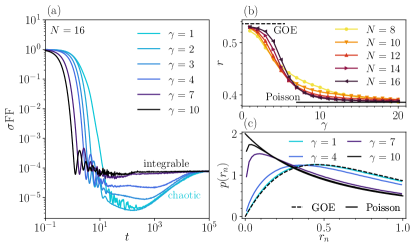
Figure 1: Dissipative quantum chaos through the SVD. (a) Singular form factor ($\sigma$FF), Eq. (3), for the XXZ model with random losses (1). For small dissipation strength a ramp is present, signaling repulsion between singular vectors, while for stronger dissipation, the correlation hole disappears, leaving only a plateau, as in the integrable case (black). (b) Ratio statistics for the singular values, computed using a portion of the smallest singular values. As the dissipation is made stronger, the average of the ratio distribution signals a crossover from chaos (GOE value) to integrability (Poisson value). (c) The crossover is also apparent in the full probability distribution of the ratios (shown for $N=16$). All the data are averaged over at least 7000 disorder realizations.

For a standard Hermitian Hamiltonian $\hat{H}$, we recall that the spectral form factor is defined as $\text{SFF}(t)=|\sum_{n}e^{-iE_{n}t}/D|^{2}$, where $\{E_{n}\}$ are the eigenenergies of $\hat{H}$, and $D$ is the Hilbert space dimension. One may also express the SFF as $\text{SFF}(t)=|\!\bra{\psi}e^{-i\hat{H}t}\ket{\psi}\!|^{2}$, i.e., as the return probability of the infinite-temperature coherent Gibbs state (CGS), $\ket{\psi}=\sum_{n}\ket{E_{n}}/\sqrt{D}$, where $\ket{E_{n}}$ are the eigenstates of $\hat{H}$. This form is particularly handy and has been used to generalize the SFF to dissipative and non-Hermitian dynamics Cornelius2022Spectral; Matsoukas2023NonHermitian. The SFF is a time-dependent quantity with distinct features at different time scales. In both integrable and chaotic systems, the ensemble-averaged SFF decays at early times and saturates to a plateau of value $1/D$ at very late times . The main difference between the chaotic and integrable behavior of the SFF is in the region between the decay and the plateau: generically, integrable systems go directly from decay to plateau, while chaotic systems exhibit a linear growth between these two regimes. This additional “ramp” stems from correlations between eigenvalues; it is visible whether or not the spectrum is unfolded Cotler2017Black; santos2020speck. More generally, a region where the SFF features values below the value of the plateau is often referred to as the correlation hole and its existence is an indication of correlations between eigenvalues.

We generalize this return probability to a NH Hamiltonian $\hat{H}$ by introducing the singular form factor ($\sigma$FF):

$$\!\!\!\sigma\text{FF}(t)=\Bigg{|}\frac{1}{D}\sum_{n}e^{-i\sigma_{n}t}\Bigg{|}^{2}=|\!\bra{\psi_{\mathrm{R}}}e^{-it\sqrt{\hat{H}^{\dagger}\hat{H}}}\ket{\psi_{\mathrm{R}}}\!|^{2}\,.$$ (3)

This extends the SFF to the NH case via the SVD: $\sigma_{n}$ are the singular values of $\hat{H}$ and $\ket{\psi_{\mathrm{R}}}=\sum_{n}\ket{v_{n}}/\sqrt{D}$ is the right infinite temperature CGS, built from its right singular vectors $\ket{v_{n}}$ (see App. B). Note that Eq. (3) can also be written in terms of the left singular vectors $\ket{u_{n}}$, replacing $\ket{\psi_{\mathrm{R}}}$ with $\ket{\psi_{\mathrm{L}}}\!=\!\sum_{n}\ket{u_{n}}/\sqrt{D}$ and $\hat{H}$ with $\hat{H}^{\dagger}$.

We argue that the $\sigma$FF is a good indicator of quantum chaos in a NH setting, being able to detect the presence of correlations among singular values. Figure 1a shows the $\sigma$FF for various disorder strengths in the considered model, Eq. (1). The $\sigma$FF exhibits a correlation hole before the plateau for small disorder. This correlation hole closes as the disorder strength gets larger, indicating the loss of correlations between the singular values.

In parallel to the form factor, the distribution of the spectral ratios $r_{n}=\min(s_{n+1},s_{n})/\max(s_{n+1},s_{n})$, where $s_{n}=E_{n+1}-E_{n}$ are the level spacings between ordered eigenvalues, is also used as a spectral probe for chaos vs integrability Oganesyan2007Localization; Atas2013Distribution. Because it involves ratios of level spacings, the density of states cancels out, removing the need for unfolding to compare systems with different global densities. Distributions of $r_{n}$ are known for the GOE, GUE, GSE and Poisson ensemble Atas2013Distribution. In our case, the relevant ensembles are: the GOE for low disorder, and the Poissonian ensemble for high disorder. The probability density distributions, $p(r_{n})$, and their average values, $r$, can be found in Ref. Atas2013Distribution.

The statistics of the singular values can also be studied via the spectral ratios defined above, replacing $E_{n}$ with $\sigma_{n}$ in the definition of the level spacing $s_{n}$ Kawabata2023Singular. This idea has recently been used to classify the singular-value statistics of NH random matrices Kawabata2023Singular, and we extend it to study the chaotic to integrable crossover. In this respect, Figs. 1b–c clearly display a crossover from GOE to Poisson statistics as the dissipation strength $\gamma$ is ramped up. In particular, Fig. 1b suggests the presence of a finite-size crossover around $\gamma_{c}/J\gtrsim 9$. In App. C we further show that, in the NH case, the results for the generalizations of the ratio statistics to complex eigenvalues Sa2020Complex are rather vague compared with the results for the singular values. Our results thus support the use of singular values statistics as a diagnostic of dissipative chaos and further point to the occurrence of a localized regime, as detailed below.

Dissipative localization of singular vectors.—The singular-value indicators presented in Fig. 1 support the presence of a localized regime in the XXZ model with random dissipation, Eq. (1). The localization induced by disorder, however, is better understood from a real-space perspective, as the name itself suggests. It is thus interesting to see whether the singular vectors of NH models display the same signatures of localization as their Hermitian counterparts (or even as NH eigenvectors).

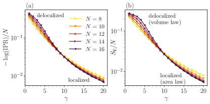
Figure 2: Dissipative localization of singular vectors. (a) The inverse participation ratio (IPR) quantifies how much a state is localized in the many-body Fock space, passing from $\mathrm{IPR}\simeq 1/D$ (delocalized) for weak dissipation to $\mathrm{IPR}\simeq 1$ (localized) for strong dissipation. Our data shows a crossover between the two regimes as the disorder in the dissipator is ramped up. (b) Entanglement entropy $S_{\mathrm{E}}$ across a bipartition of the chain in two halves. For small dissipation $\gamma$, $S_{\mathrm{E}}$ increases at least with the system size $N$ (volume law, delocalized states), while at larger $\gamma$ the entanglement entropy decreases with system size when divided by $N$, thus suggesting an area law of entanglement (localized states). The data are averaged over at least 7000 disorder realizations.

For a single particle, the eigenstates of a Hermitian and localized Hamiltonian have a well-understood real-space structure. Each eigenstate $\ket{E_{n}}$ is concentrated around its localization center $\mathbf{x}_{n}$, and its decaying profile is characterized by a localization length $\xi$, namely $\innerproduct{\mathbf{x}}{E_{n}}\sim e^{-|\mathbf{x}-\mathbf{x}_{n}|/\xi}$. A similar situation takes place in single-particle, NH, localized Hamiltonians, where the disorder-induced localization competes with the localization yielded by the non-Hermitian skin effect Hatano1996Localization; Hatano1997Vortex; Hatano1998NonHermitian.

In the many-body case, the situation is more complicated. Even in the Hermitian setup, there seems to be no simple localization in Hilbert space DeLuca2013Ergodicity. Rather, the eigenstates of MBL Hamiltonians are believed to be also eigenstates of local integrals of motion (LIOMS) Serbyn2013Local; Ros2015Integrals; Imbrie2016Diagonalization; Imbrie2016Local and to obey the area law of entanglement Abanin2019Colloquium.

Previous works have studied some aspects of NH, localized, many-body eigenvectors, e.g., identifying a crossover from volume to area law for the entanglement entropy Hamazaki2019NonHermitian. Here, we perform a similar analysis, though using the singular vectors of NH models, which, we recall, form an orthonormal basis for the Hilbert space, contrary to the eigenvectors. Thus, we show that the SVD allows discerning between localized and ergodic regimes even at the level of singular vectors; this extends the use of the SVD beyond diagnosing dissipative chaos Kawabata2023Singular.

For simplicity, we use two commonly considered indicators: the inverse participation ratio (IPR) and the entanglement entropy across a bipartition. Our analysis is based on the right singular vectors, the left ones yielding similar results.

The IPR of singular vectors is defined as the ensemble average of $\sum_{k=1}^{D}|\!\innerproduct{e_{k}}{v_{n}}\!|^{4}/D$, where $\{\ket{e_{k}}\}$ is the computational basis and $\ket{v_{n}}$ are the (right) singular vectors. It is expected that $\mathrm{IPR}\approx 1/D$ for delocalized states (as obtained for $\ket{v_{n}}$ uniformly spread over the computational basis), while $\mathrm{IPR}\approx 1$ if $\ket{v_{n}}$ is localized on a single Fock state. Figure 2a presents the logarithm of the IPR of singular vectors, scaled with system size: our data shows the presence of a finite-size crossover from delocalized to localized singular vectors around a value $\gamma_{c}/J\approx 9$, consistent with the picture extracted from the average gap ratio ($r$-parameter) statistics.

We further present our results for the entanglement entropy across a bipartition in Fig. 2b. Recall that, for a generic state $\ket{\psi}$, the entanglement entropy is defined as $S_{\mathrm{E}}=-\tr\rho_{A}\log\rho_{A}$, where $\rho_{A}=\Tr_{B}(\outerproduct{\psi}{\psi})$ and $A\cup B$ form a bipartition of the chain in two intervals. As for the IPR, the entanglement entropy supports the presence of a localized regime: it crosses over from a volume law at small dissipation to an area law at large dissipation, again consistently indicating a critical value $\gamma_{c}/J\approx 9$ for the system sizes considered. Remarkably, the same analysis of the IPR and entanglement entropy with the eigenvectors does not display such a clear crossover, thus strongly motivating the use of the SVD (see App. D). While a weak, inhomogeneous dissipation breaks the integrability of the XXZ chain making it (dissipatively) chaotic, more disordered losses localize it again and restore integrability.

Conclusions.—We have investigated the role of a disordered dissipative term on an otherwise clean, integrable, interacting quantum system. Adding such a term makes the system evolve under an effective non-Hermitian (NH) Hamiltonian, physically representing the average evolution of quantum trajectories conditioned to no quantum jumps. The eigendecomposition of NH Hamiltonians yields complex eigenvalues and non-orthogonal (left and right) eigenvectors. We argued in favor of using the singular value decomposition (SVD) and showed that, indeed, the singular values can be used to detect a crossover from chaotic to integrable spectral features, and the singular vectors to probe a crossover from delocalization to localization. The crossover takes place at the dissipation strength $\gamma_{c}/J\approx 9$, which is comparable to the Hermitian critical disorder strength $h_{c}/J\approx 4$ seen in finite-size numerics, once one realizes that $\gamma_{i}\in[0,\gamma]$ is half the width of the interval $h_{i}\in[-h,h]$. As additional tools to study the singular value statistics, we introduced the singular form factor ($\sigma$FF). We showed that the $\sigma$FF features a correlation hole when the dissipative disorder is weak, and that the correlation hole closes for large dissipative disorder.

Despite providing an effective description of the time evolution of open systems, NH Hamiltonians do not capture all the features of open system dynamics, e.g., the entanglement behavior. In this setting, random dissipation-induced localization points to a quantum dynamics that is highly sensitive to the effect of inhomogeneities. This contrasts with a homogeneous dissipation which, in our case, does not induce localization.

A crucial point, in the Hermitian setting, is how the chaotic/localized crossover scales with system size. For the dissipative case, this is not as relevant because the NH evolution describes an exponentially small (in system size and time) fraction of trajectories. In turn, our findings are meaningful precisely for small systems size: only in this case the chaotic/localized behaviors can be actually observed in experiments. Our results are thus relevant for noisy intermediate-scale quantum (NISQ) devices Preskill2018Quantum, since we show that the Hamiltonian properties are significantly altered by disordered dissipation.

Acknowledgments.—We thank Masahito Ueda for useful discussions, and Oskar A. Prośniak and Pablo Martínez-Azcona for careful reading of the manuscript. F.B. thanks Carlo Vanoni for illuminating discussions on localization indicators. This research was funded in part by the Luxembourg National Research Fund (FNR, Attract grant 15382998), the John Templeton Foundation (Grant 62171), and the QuantERA II Programme that has received funding from the European Union’s Horizon 2020 research and innovation programme (Grant 16434093). The opinions expressed in this publication are those of the authors and do not necessarily reflect the views of the John Templeton Foundation. The numerical simulations presented in this work were in part carried out using the HPC facilities of the University of Luxembourg.

Appendix A Effective Non-Hermitian Hamiltonians

Several theoretical frameworks have been developed to describe the dynamics of open quantum systems: quantum trajectories Brun2002Simple, Zwanzig-Mori projection operators ZwanzigPhysRev1961 and collision models Ciccarello2022Quantum to name a few. Here, we perform the common assumptions of having an infinitely large Markovian bath, with a fast relaxation timescale compared to that of the system, to which it is weakly coupled. Formally, this is reflected in the possibility of writing down a Gorini–Kossakowski–Sudarshan–Lindblad (GKSL) master equation for the reduced density matrix $\rho_{t}$ of the system:

$$\dot{\rho}_{t}=-i[\hat{H},\rho_{t}]+\sum_{j}\mathcal{D}[\sqrt{\gamma_{j}}\hat{L}_{j}]\rho_{t}\,,$$ (4)

with the dissipator $\mathcal{D}[\hat{\mathcal{O}}]\rho=\hat{\mathcal{O}}\rho\hat{\mathcal{O}}^{\dagger}-\tfrac{1}{2}\{\hat{\mathcal{O}}^{\dagger}\hat{\mathcal{O}},\rho\}$. Above, the Hermitian Hamiltonian $\hat{H}$ describes the dynamics of the system alone, while the interaction with the bath is encoded in the jump operators $\hat{\mathcal{O}}=\sqrt{\gamma_{j}}\hat{L}_{j}$, $\gamma_{j}>0$. The introduction of an effective non-Hermitian Hamiltonian,

$$\hat{H}_{\text{eff}}=\hat{H}-\frac{i}{2}\sum_{j}\gamma_{j}\hat{L}_{j}^{\dagger}\hat{L}_{j},$$ (5)

allows re-writing the GKSL equation as

$$\dot{\rho}_{t}=-i(\hat{H}_{\text{eff}}\rho_{t}-\rho_{t}\hat{H}_{\text{eff}}^{\dagger})+\sum_{j}\gamma_{j}\hat{L}_{j}\rho_{t}\hat{L}_{j}^{\dagger}.$$ (6)

This equation separates the density matrix evolving under $\hat{H}_{\text{eff}}$ from the jump terms. The case we describe in the main text, Eq. (1), is a NH Hamiltonian and corresponds to a dynamics with no jumps; the dynamics is then governed by the effective Hamiltonian only.

Two important remarks are in order. First, the use of the GKSL equation automatically implies that an average over the bath influence is taken at the level of the density matrix. This fact implies that quantities that are non-linear in the density matrix, like entanglement, are not well captured within the GKSL framework Li2018Quantum; Skinner2019Measurement. Second, no-jump trajectories constitute an exponentially small fraction (both in time and in the system size) of all the quantum trajectories since, at each time and for each spin, one needs to impose that no jump occurs: these events are typically independent and their probabilities multiply. Despite these two caveats, we nevertheless study a many-body system under strong local dissipation, and moreover focus on the MBL transition, which is usually linked to entanglement properties. This might seem a contradiction, but it is only an apparent one. Indeed, the use of non-Hermitian Hamiltonians has already been shown to capture well entanglement transitions in many-body quantum systems Biella2021Many; Turkeshi2021Measurement; Youenn2023Volume. Additionally, averaging the density matrix before computing the entanglement is reminiscent of the annealed average usually considered in disordered systems Mezard1987Spin, which provides an approximation that, in certain cases, is also accurate.

Appendix B General properties of the eigen- and singular value decomposition

Here, we briefly review some known properties of the eigen- and singular-value decompositions of Hermitian and non-Hermitian Hamiltonians. We interchangeably refer to the matrix representation of our Hamiltonian in some basis simply as the “Hamiltonian”, as we focus on a finite-dimensional Hilbert space of dimension $D$. To fix the ideas, one can take the Hamiltonian $\hat{H}$ to describe the XXZ spin chain, Eq. (2a), in the zero magnetization sector, corresponding to $D=\binom{N}{N/2}$.

B.1 Remarks on the eigendecomposition

Consider a Hermitian Hamiltonian $H$ (we drop the hat as we refer to its matrix representation). It can be diagonalized as $H=W\Lambda W^{\dagger}=\sum_{n}E_{n}\outerproduct{w_{n}}{w_{n}}$ though a single unitary transformation, $W=(\ket{w_{1}},\ldots,\ket{w_{\textsc{d}}})$, $\Lambda=\operatorname{diag}(E_{1},\ldots,E_{\textsc{d}})$ being the diagonal matrix formed by the real eigenvalues. The eigenstates of $H$, $\{\ket{w_{n}}\}$, are orthogonal and can be made orthonormal; so, they resolve the identity, $\mathbb{1}_{\textsc{d}}=\sum_{n}\outerproduct{w_{n}}{w_{n}}$. The eigenvalues and eigenstates of a Hermitian operator $H$ have a physical meaning in quantum mechanics, being respectively the outcomes of the measurements of $H$ and the corresponding states the system collapses to after the measurement.

In turn, a non-Hermitian Hamiltonian $H\neq H^{\dagger}$ is not guaranteed to be diagonalizable. The lack of diagonalizability comes from a degeneracy of eigenvalues and eigenvectors, at what are known as exceptional points Miri2019Exceptional. Away from these degeneracies, we can assume $H$ to be diagonalizable, although its eigenvectors are in general not orthogonal and its eigenvalues can be complex. A way out of this, that has been intensely used in the non-Hermitian physics literature Brody2014Biorthogonal, is to use both the right and left eigenvectors of $H$, satisfying $H\ket{R_{n}}=E_{n}\ket{R_{n}}$ and $\bra{L_{n}}H=E_{n}\bra{L_{n}}$, respectively. These are not orthonormal sets themselves, as $\innerproduct{R_{n}}{R_{m}}\neq\delta_{nm}$ (same with $L$), but are biorthogonal, i.e., $\innerproduct{L_{n}}{R_{m}}=c\,\delta_{nm}$. The constant $c$ can be set to one to make the right and left eigenvectors biorthonormal. This way, the identity can be resolved as $\mathbb{1}_{\textsc{d}}=\sum_{n}\outerproduct{R_{n}}{L_{n}}$. Note that, if the right and left eigenvectors are biorthonormal, one can still normalize the right ones but not the left ones, and vice versa. Assuming biorthonormality, one can make the decomposition $H=R\Lambda L^{\dagger}=\sum_{n}E_{n}\outerproduct{R_{n}}{L_{n}}$, where $R=(\ket{R_{1}},\ldots,\ket{R_{\textsc{d}}})$ and $L=(\ket{L_{1}},\ldots,\ket{L_{\textsc{d}}})$ are the non-unitary transformations that make $H$ diagonal, and where the eigenvalues $E_{n}$ are now generally complex.

B.2 Brief review of the singular value decomposition

Any Hamiltonian $H$, be it Hermitian or non-Hermitian, can be decomposed through the singular value decomposition (SVD) into $H=U\Sigma V^{\dagger}=\sum_{j}\sigma_{n}\outerproduct{u_{n}}{v_{n}}$, where $U=(\ket{u_{1}},\ldots,\ket{u_{\textsc{d}}})$ and $V=(\ket{v_{1}},\ldots,\ket{v_{\textsc{d}}})$ are unitaries whose columns are the left and right singular vectors, respectively, and $\Sigma=\operatorname{diag}(\sigma_{1},\ldots,\sigma_{\textsc{d}})$ is the positive semi-definite matrix of singular values. As $U$ and $V$ are unitaries, their columns are orthonormal and resolve the identity without any need to recur to bi-orthogonality.

The SVD makes explicit how a general matrix $H$ acts on an orthonormal basis $V$, to get a rotated orthonormal basis $U$ stretched or compressed by the real and non-negative numbers in the diagonal of $\Sigma$. From an operational point of view, one can obtain the SVD of a matrix by using an eigendecomposition procedure. The basis $V$ is the orthonormal eigenbasis of the Hermitian matrix $H^{\dagger}H$ with eigenvalues $\{\sigma_{n}^{2}\}$, while the orthonormal basis $U$ is the eigenbasis of the Hermitian matrix $HH^{\dagger}$, sharing the same eigenvalues. By standard manipulations in linear algebra, one can see that the SVD of a matrix $H$ can also be obtained from the eigendecomposition of the cyclic matrix

$$C=\begin{pmatrix}\mathbb{0}&H\\ H^{\dagger}&\mathbb{0}\end{pmatrix}.$$ (7)

$C$ is a $2D\times 2D$ matrix with eigenvalues $\{\pm\sigma_{n}\}$, associated to eigenvectors $(\pm u_{n},v_{n})^{T}/\sqrt{2}$.

It is important to stress that the two procedures described above to obtain the SVD of a matrix from eigendecomposition routines are equivalent in principle, but different in practice. The use of either $H^{\dagger}H$ or $HH^{\dagger}$ does not increase the matrix dimension, but yields the singular values squared. This results in a loss of precision, which is particularly severe for the small singular values—which are the ones that we used in the main text. On the other hand, the cyclic matrix $C$ provides directly the singular values $\sigma$, albeit with a doubled computational cost (typically, one gets both $\sigma_{n}$ and $-\sigma_{n}$), and with the caveat that the small $\sigma_{n}$’s lie at the center of the spectrum of $C$—and procedures as shift-invert or polynomial filtering must be used.

Appendix C Complex spectral gap ratios

In the case of an effective open system Hamiltonian such as Eq. (5) the spectrum is complex and there is no clear notion of ordering the eigenvalues. One can nevertheless find the nearest neighbor $E_{n}^{\textsc{nn}}$ of each eigenvalue $E_{n}$ on the complex plane, defined as the eigenvalue $E_{n}^{\textsc{nn}}$ which satisfies $|E_{n}^{\textsc{nn}}-E_{n}|=\min_{m\neq n}|E_{n}-E_{m}|$. As explained in the main text, to avoid the need to unfold the spectrum, we would like to consider a ratio of energy-dependent quantities. A natural other such quantity would be the next-nearest neighbor $E_{n}^{\textsc{nnn}}$ for each eigenvalue, which would amount to ordering the set $\{|E_{m}-E_{n}|\}_{m\neq n}$ and selecting the second entry to find $E_{n}^{\textsc{nnn}}$. The spectral ratio to be studied is then the complex ratio Sa2020Complex

$$z_{n}\equiv\frac{E_{n}^{\textsc{nn}}-E_{n}}{E_{n}^{\textsc{nnn}}-E_{n}}~{}.$$ (8)

Note that this definition is similar but not the same as the ratio of closest-neighbor and 2nd closest-neighbor defined in Ref. Srivastava2018Ordered for real eigenvalues. In that work the ratio of the absolute value of the difference between levels (=distance) was considered, while in the definition (8) it is not the ratio of distances which is computed, but rather the ratio of differences. More specifically, the ratio for real eigenvalues defined in Ref. Srivastava2018Ordered gets values between 0 and 1, while the definition (8), restricted to real eigenvalues, gets values between $-1$ and $1$.

As in the Hermitian case, it is often useful to extract a single number from the ratio statistics as a probe to the type of spectrum. In the complex case $z_{n}=r_{n}e^{i\theta_{n}}$ with $0\leq r_{n}\leq 1$ because $|E_{n}^{\textsc{nn}}-E_{n}|\leq|E_{n}^{\textsc{nnn}}-E_{n}|$. One such single-number probe would be the averages $r=\langle r_{n}\rangle$ and $\cos\theta=\langle\cos\theta_{n}\rangle$. Table 1 shows the values expected from uncorrelated complex eigenvalues (Poisson ensemble) and random matrix ensembles, as reported in Ref. Sa2020Complex. The Ginibre Unitary Ensemble (GinUE) are complex matrices with independent identically distributed complex entries taken from a Gaussian distribution and setting $\beta=2$ in the joint eigenvalue distribution. The Toric Unitary Ensemble (TUE) is a generalization of the Circular Unitary Ensemble (where eigenvalues lay on a circle) to the complex plane compactified into a torus (such that all eigenvalues lay on the torus). The next Appendix discusses this single-number probe in our model.

	Poisson	GinUE	TUE
$r$	2/3	0.73810	0.7315 – 0.73491
$-\cos\theta$	0	0.24051	0.15322 – 0.1938

Table 1: Average values expected for $\langle r_{n}\rangle$ and $-\langle\cos\theta_{n}\rangle$ for different types of complex eigenvalue statistics, taken from Ref. Sa2020Complex.

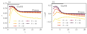
Figure 3: Eigenvalue statistics for the XXZ model with random losses using complex gap ratio statistics. (a) The average value of the norm of the complex gap ratios. (b) Cosine of the phase of the complex gap ratios. The data was extracted from a small window in the middle of the (complex) spectrum and averaged over at least 7000 disorder realizations.

Appendix D Further results for the XXZ model with random losses

In the main text, we studied the singular-value, real, spectral ratio statistics for the model (1) and found that they show a clear crossover from GOE to Poisson, see Fig. 1. Let us now present the eigenvalue statistics using the complex spectral gap ratios as described in Appendix C. Figure 3 displays the gap ratio statistics for the complex eigenvalues of the XXZ model with dissipative disorder, Eq. (1), as a function of the disorder strength $\gamma$. As we show in Fig. 3, the results for $r$ and $\cos\theta$ do not provide clear-cut values which we could clearly attribute to a crossover from chaos to integrability. Also, the behavior of these single-number statistics does not change smoothly with the system size $N$, in contrast with the behavior of the single-number statistics for the singular values.

We show our study on the localization indicators for the (right) eigenvectors of the NH XXZ model (1), see Fig. 4. For the entanglement entropy, we use the definition $S_{\mathrm{E}}=-\tr\rho_{A}\log\rho_{A}$ with $\rho_{A}=\Tr_{B}(\outerproduct{R_{n}}{R_{n}})$, i.e., using the right eigenvectors only Hamazaki2019NonHermitian. In principle, both right and left eigenvectors could be used to construct the reduced density matrix lu2023unconventional, even if the physical difference between the various cases is not yet well understood. Even with a rescaling with the system size, a crossover between a delocalized/localized regime for the eigenvectors does not occur (contrary to what we see for singular vectors). This supports even more the use of the SVD as a tool to generalize standard Hermitian phenomena, as already motivated in totally different settings HerviouPRA2019; BrunelliSciPost2023.

Finally, in the main text, we showed the localization crossover captured by the scaled IPR and entanglement entropy. Here, we further show the same results, without the system-size rescaling in Fig. 5a–b, which masks the crossover, but clearly show the transition between volume law to area law, Fig. 5c.

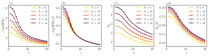
Figure 4: Localization indicators for the right eigenvectors of the XXZ model with random losses. (a) and (c): IPR and entanglement entropy of the right eigenvectors the XXZ model with random losses, respectively. (b) and (d), same plots including a scaling with system size. We see that no delocalization/localization crossover at finite size occurs for the eigenvectors. The data was extracted from a small window in the middle of the (complex) spectrum and averaged over at least 7000 disorder realizations.

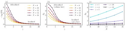
Figure 5: Dissipative localization of singular vectors (without rescaling) of the XXZ model with random losses. Here we plot the same data shown in Fig. 2 (main text) without rescaling by system size. (a) The inverse participation ratio (IPR) quantifies how much a state is localized in the many-body Fock space, passing from $\mathrm{IPR}\simeq 1/D$ (delocalized) for weak dissipation to $\mathrm{IPR}\simeq 1$ (localized) for strong dissipation. Our data shows a crossover between the two regimes as the disorder in the dissipator is ramped up. (b) Entanglement entropy across a bipartition of the chain in two halves. A delocalized regime is visible for small dissipation $\gamma$, while localization takes place at larger $\gamma$. (c) The entanglement entropy changes from a volume law $S_{\mathrm{E}}\propto N$ (small $\gamma$), to an area law $S_{\mathrm{E}}\sim\mathrm{const.}$ (large $\gamma$). All the data was extracted from a small window in the middle of the spectrum and averaged over at least 7000 disorder realizations.

Appendix E Results for the interacting Hatano-Nelson model

Here we perform the same analysis described in the main text for the interacting Hatano-Nelson model

$$\hat{H}=J\sum_{i}\left[\frac{1}{2}\left(e^{g}\hat{S}_{i}^{+}\hat{S}_{i+1}^{-}+e^{-g}\hat{S}_{i}^{-}\hat{S}_{i+1}^{+}\right)+\Delta\hat{S}_{i}^{z}\hat{S}_{i+1}^{z}\right]+\sum_{i}h_{i}\hat{S}_{i}^{z}.$$ (9)

This model was studied in Ref. Hamazaki2019NonHermitian, where it was shown it hosts a NH MBL phase. Here, we study its localization properties through the lens of the SVD. We fix, as for the model in the main text, $J=1$ and $\Delta=1$, and further set $g=0.1$. Then, we extract the disordered fields $h_{i}\in[-h,h]$ according to the uniform distribution. In order to avoid the NH skin effect, which may be mistaken for localization, we use periodic boundary conditions.

In contrast with the Hamiltonian considered in the main text, Eq. (1), where non-Hermiticity and disorder coincide, the non-Hermiticity in the interacting Hatano-Nelson model, Eq. (9), comes from the unbalanced hoppings while the randomness comes from a standard (Hermitian) local field. Therefore, in this model, localization and chaos are not induced by non-Hermiticiy, but one can quantify their resilience to non-Hermiticity.

The singular form factor and the singular value statistics for the interacting Hatano-Nelson model, Eq. (9), as function of disorder strength $h$, are shown in Fig. 6. The localization properties of the singular vectors, as quantified by the IPR and the entanglement entropy, are plotted as a function of $h$ in Figs. 7–8.

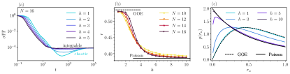
Figure 6: Singular value statistics for the interacting Hatano-Nelson model with $g=0.1$ and $J=1=\Delta$. (a) The $\sigma$FF shows that as $h$ increases correlations among the singular values disappear and the correlation hole closes. (b) The average of the ratio distributions, for data taken from the smallest singular values, shows a clear crossover from the GOE (chaotic) value to the Poisson (integrable) value as $h$ is increased, with the transition around $h/J\approx 4$. (c) The ratio statistics follow the distribution expected from the GOE for a small value of $h$, and that expected from the Poissonian ensemble for a large value of $h$ (shown for $N=16$). All data is averaged over at least 5000 realizations of the disorder.

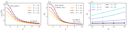
Figure 7: Dissipative localization of singular vectors for the interacting Hatano-Nelson model. (a) The IPR as a function of $h$, plotted for several system sizes $N$. For all $N$’s, the IPR shows a crossover from delocalized singular vectors to localized singular vectors as $h$ increases. (b) The entanglement entropy of the singular vectors as a function of $h$, for the same system sizes. Also $S_{E}$ shows a clear crossover between delocalization (volume law) and localization (area law) as $h$ is increased. (c) The crossover from $S_{E}\propto N$ (volume law) to $S_{E}\sim\mathrm{const.}$ (area law) as $h$ is increased, now plotted as a function of the system size $N$. All data is averaged over at least 5000 realizations of the disorder.

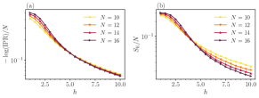
Figure 8: Dissipative localization of singular vectors for the interacting Hatano-Nelson model (with rescaling). Same data as in Fig. 7, where both (a) the IPR and (b) the entanglement entropy are rescaled with system size to highlight the crossover.

References

- Bohigas et al. (1984) O. Bohigas, M. J. Giannoni, and C. Schmit, Phys. Rev. Lett. 52, 1 (1984).
- Deutsch (1991) J. M. Deutsch, Phys. Rev. A 43, 2046 (1991).
- Srednicki (1994) M. Srednicki, Phys. Rev. E 50, 888 (1994).
- Haake (2010) F. Haake, Quantum Signatures of Chaos (Springer, Berlin, Heidelberg, 2010).
- Anderson (1958) P. W. Anderson, Phys. Rev. 109, 1492 (1958).
- Gornyi et al. (2005) I. V. Gornyi, A. D. Mirlin, and D. G. Polyakov, Phys. Rev. Lett. 95, 206603 (2005).
- Basko et al. (2006) D. M. Basko, I. L. Aleiner, and B. L. Altshuler, Ann. Phys. (Amsterdam) 321, 1126 (2006).
- Oganesyan and Huse (2007) V. Oganesyan and D. A. Huse, Phys. Rev. B 75, 155111 (2007).
- Žnidarič et al. (2008) M. Žnidarič, T. Prosen, and P. Prelovšek, Phys. Rev. B 77, 064426 (2008).
- Pal and Huse (2010) A. Pal and D. A. Huse, Phys. Rev. B 82, 174411 (2010).
- Bardarson et al. (2012) J. H. Bardarson, F. Pollmann, and J. E. Moore, Phys. Rev. Lett. 109, 017202 (2012).
- Altshuler et al. (2009) B. Altshuler, H. Krovi, and J. Roland, arXiv:0908.2782 (2009).
- Altshuler et al. (2010) B. Altshuler, H. Krovi, and J. Roland, Proc. Natl. Acad. Sci. (USA) 107, 12446 (2010).
- Laumann et al. (2015) C. R. Laumann, R. Moessner, A. Scardicchio, and S. L. Sondhi, Europ. Phys. J. Special Topics 224, 75 (2015).
- Serbyn et al. (2013) M. Serbyn, Z. Papić, and D. A. Abanin, Phys. Rev. Lett. 111, 127201 (2013).
- Ros et al. (2015) V. Ros, M. Müller, and A. Scardicchio, Nucl. Phys. B891, 420 (2015).
- Imbrie (2016) J. Z. Imbrie, Phys. Rev. Lett. 117, 027201 (2016).
- Imbrie et al. (2017) J. Z. Imbrie, V. Ros, and A. Scardicchio, Ann. Phys. (Berlin) 529, 1600278 (2017).
- D’Alessio et al. (2016) L. D’Alessio, Y. Kafri, A. Polkovnikov, and M. Rigol, Adv. Phys. 65, 239 (2016).
- Alet and Laflorencie (2018) F. Alet and N. Laflorencie, Comptes Rendus Physique 19, 498 (2018).
- Abanin et al. (2019) D. A. Abanin, E. Altman, I. Bloch, and M. Serbyn, Rev. Mod. Phys. 91, 021001 (2019).
- Schreiber et al. (2015) M. Schreiber, S. S. Hodgman, P. Bordia, H. P. Lüschen, M. H. Fischer, R. Vosk, E. Altman, U. Schneider, and I. Bloch, Science 349, 842 (2015).
- Smith et al. (2016) J. Smith, A. Lee, P. Richerme, B. Neyenhuis, P. W. Hess, P. Hauke, M. Heyl, D. A. Huse, and C. Monroe, Nat. Phys. 12, 907 (2016).
- Lukin et al. (2019) A. Lukin, M. Rispoli, R. Schittko, M. E. Tai, A. M. Kaufman, S. Choi, V. Khemani, J. Léonard, and M. Greiner, Science 364, 256 (2019).
- Huse et al. (2013) D. A. Huse, R. Nandkishore, V. Oganesyan, A. Pal, and S. L. Sondhi, Phys. Rev. B 88, 014206 (2013).
- Chandran et al. (2014) A. Chandran, V. Khemani, C. R. Laumann, and S. L. Sondhi, Phys. Rev. B 89, 144201 (2014).
- Parameswaran and Vasseur (2018) S. A. Parameswaran and R. Vasseur, Rep. Prog. Phys. 81, 082501 (2018).
- Khemani et al. (2016) V. Khemani, A. Lazarides, R. Moessner, and S. L. Sondhi, Phys. Rev. Lett. 116, 250401 (2016).
- Sachdev (2011) S. Sachdev, Quantum Phase Transitions, 2nd ed. (Cambridge University Press, 2011).
- Li et al. (2018) Y. Li, X. Chen, and M. P. A. Fisher, Phys. Rev. B 98, 205136 (2018).
- Skinner et al. (2019) B. Skinner, J. Ruhman, and A. Nahum, Phys. Rev. X 9, 031009 (2019).
- Matsumoto et al. (2022) N. Matsumoto, M. Nakagawa, and M. Ueda, Phys. Rev. Res. 4, 033250 (2022).
- Kawabata et al. (2022) K. Kawabata, K. Shiozaki, and S. Ryu, Phys. Rev. B 105, 165137 (2022).
- Hatano and Nelson (1996) N. Hatano and D. R. Nelson, Phys. Rev. Lett. 77, 570 (1996).
- Hatano and Nelson (1997) N. Hatano and D. R. Nelson, Phys. Rev. B 56, 8651 (1997).
- Hatano and Nelson (1998) N. Hatano and D. R. Nelson, Phys. Rev. B 58, 8384 (1998).
- Goldsheid and Khoruzhenko (1998) I. Y. Goldsheid and B. A. Khoruzhenko, Phys. Rev. Lett. 80, 2897 (1998).
- Kawabata and Ryu (2021) K. Kawabata and S. Ryu, Phys. Rev. Lett. 126, 166801 (2021).
- Cornelius et al. (2022) J. Cornelius, Z. Xu, A. Saxena, A. Chenu, and A. del Campo, Phys. Rev. Lett. 128, 190402 (2022).
- Kawabata et al. (2023a) K. Kawabata, A. Kulkarni, J. Li, T. Numasawa, and S. Ryu, PRX Quantum 4, 030328 (2023a).
- De Tomasi and Khaymovich (2022) G. De Tomasi and I. M. Khaymovich, Phys. Rev. B 106, 094204 (2022).
- De Tomasi and Khaymovich (2023a) G. De Tomasi and I. M. Khaymovich, arXiv:2311.00019 (2023a).
- De Tomasi and Khaymovich (2023b) G. De Tomasi and I. M. Khaymovich, arXiv:2302.00015 (2023b).
- Hamazaki et al. (2019) R. Hamazaki, K. Kawabata, and M. Ueda, Phys. Rev. Lett. 123, 090603 (2019).
- Zhai et al. (2020) L.-J. Zhai, S. Yin, and G.-Y. Huang, Phys. Rev. B 102, 064206 (2020).
- Suthar et al. (2022) K. Suthar, Y.-C. Wang, Y.-P. Huang, H. H. Jen, and J.-S. You, Phys. Rev. B 106, 064208 (2022).
- Ghosh et al. (2022) S. Ghosh, S. Gupta, and M. Kulkarni, Phys. Rev. B 106, 134202 (2022).
- Hamazaki et al. (2022) R. Hamazaki, M. Nakagawa, T. Haga, and M. Ueda, arXiv:2206.02984 (2022).
- Sá et al. (2020) L. Sá, P. Ribeiro, and T. Prosen, Phys. Rev. X 10, 021019 (2020).
- Brody (2013) D. C. Brody, J. Phys. A 47, 035305 (2013).
- Herviou et al. (2019) L. Herviou, J. H. Bardarson, and N. Regnault, Phys. Rev. A 99, 052118 (2019).
- Porras and Fernández-Lorenzo (2019) D. Porras and S. Fernández-Lorenzo, Phys. Rev. Lett. 122, 143901 (2019).
- Brunelli et al. (2023) M. Brunelli, C. C. Wanjura, and A. Nunnenkamp, SciPost Phys. 15, 173 (2023).
- Kawabata et al. (2023b) K. Kawabata, Z. Xiao, T. Ohtsuki, and R. Shindou, PRX Quantum 4, 040312 (2023b).
- Luitz et al. (2015) D. J. Luitz, N. Laflorencie, and F. Alet, Phys. Rev. B 91, 081103 (2015).
- Bertrand and García-García (2016) C. L. Bertrand and A. M. García-García, Phys. Rev. B 94, 144201 (2016).
- Sierant and Zakrzewski (2019) P. Sierant and J. Zakrzewski, Phys. Rev. B 99, 104205 (2019).
- Šuntajs et al. (2020) J. Šuntajs, J. Bonča, T. Prosen, and L. Vidmar, Phys. Rev. E 102, 062144 (2020).
- Panda et al. (2020) R. K. Panda, A. Scardicchio, M. Schulz, S. R. Taylor, and M. Žnidarič, Europhys. Lett. 128, 67003 (2020).
- Abanin et al. (2021) D. Abanin, J. Bardarson, G. De Tomasi, S. Gopalakrishnan, V. Khemani, S. Parameswaran, F. Pollmann, A. Potter, M. Serbyn, and R. Vasseur, Ann. Phys. (Amsterdam) 427, 168415 (2021).
- Morningstar et al. (2022) A. Morningstar, L. Colmenarez, V. Khemani, D. J. Luitz, and D. A. Huse, Phys. Rev. B 105, 174205 (2022).
- Minganti et al. (2019) F. Minganti, A. Miranowicz, R. W. Chhajlany, and F. Nori, Phys. Rev. A 100, 062131 (2019).
- Ciccarello et al. (2022) F. Ciccarello, S. Lorenzo, V. Giovannetti, and G. M. Palma, Phys. Rep. 954, 1 (2022).
- Breuer and Petruccione (2007) H.-P. Breuer and F. Petruccione, The Theory of Open Quantum Systems (Oxford University Press, Oxford, 2007).
- Kunst et al. (2018) F. K. Kunst, E. Edvardsson, J. C. Budich, and E. J. Bergholtz, Phys. Rev. Lett. 121, 026808 (2018).
- Yao et al. (2018) S. Yao, F. Song, and Z. Wang, Phys. Rev. Lett. 121, 136802 (2018).
- Trefethen and Bau (1997) L. N. Trefethen and D. Bau, III, Numerical Linear Algebra (SIAM, Philadelphia, PA, 1997).
- Ramos et al. (2021) T. Ramos, J. J. García-Ripoll, and D. Porras, Phys. Rev. A 103, 033513 (2021).
- Gómez-León et al. (2023) Á. Gómez-León, T. Ramos, A. González-Tudela, and D. Porras, Quantum 7, 1016 (2023).
- Mehta (2004) M. L. Mehta, Random Matrices (Elsevier, 2004).
- Berry and Tabor (1977) M. V. Berry and M. Tabor, Proc. R. Soc. London A 356, 375 (1977).
- Leviandier et al. (1986) L. Leviandier, M. Lombardi, R. Jost, and J. P. Pique, Phys. Rev. Lett. 56, 2449 (1986).
- Wilkie and Brumer (1991) J. Wilkie and P. Brumer, Phys. Rev. Lett. 67, 1185 (1991).
- Alhassid and Levine (1992) Y. Alhassid and R. D. Levine, Phys. Rev. A 46, 4650 (1992).
- Ma (1995) J.-Z. Ma, J. Phys. Soc. Japan 64, 4059 (1995).
- Cotler et al. (2017) J. S. Cotler, G. Gur-Ari, M. Hanada, J. Polchinski, P. Saad, S. H. Shenker, D. Stanford, A. Streicher, and M. Tezuka, J. High Energy Phys. 2017, 118 (2017).
- del Campo et al. (2017) A. del Campo, J. Molina-Vilaplana, and J. Sonner, Phys. Rev. D 95, 126008 (2017).
- Chenu et al. (2018) A. Chenu, I. L. Egusquiza, J. Molina-Vilaplana, and A. del Campo, Sci. Rep. 8, 12634 (2018).
- Xu et al. (2021) Z. Xu, A. Chenu, T. Prosen, and A. del Campo, Phys. Rev. B 103, 064309 (2021).
- Shir et al. (2023) R. Shir, P. Martinez-Azcona, and A. Chenu, arXiv:2311.09292 (2023).
- Atas et al. (2013) Y. Y. Atas, E. Bogomolny, O. Giraud, and G. Roux, Phys. Rev. Lett. 110, 084101 (2013).
- Matsoukas-Roubeas et al. (2023) A. S. Matsoukas-Roubeas, F. Roccati, J. Cornelius, Z. Xu, A. Chenu, and A. del Campo, J. High Energy Phys. 2023, 60 (2023).
- Note (1) Here we are assuming that the energies have no special relations among themselves, as is generically expected in many-body, interacting quantum systems.
- Santos et al. (2020) L. F. Santos, F. Pérez-Bernal, and E. J. Torres-Herrera, Phys. Rev. Res. 2, 043034 (2020).
- Luca and Scardicchio (2013) A. D. Luca and A. Scardicchio, Europhys. Lett. 101, 37003 (2013).
- Preskill (2018) J. Preskill, Quantum 2, 79 (2018).
- Brun (2002) T. A. Brun, Am. J. Phys. 70, 719 (2002).
- Zwanzig (1961) R. Zwanzig, Phys. Rev. 124, 983 (1961).
- Biella and Schiró (2021) A. Biella and M. Schiró, Quantum 5, 528 (2021).
- Turkeshi et al. (2021) X. Turkeshi, A. Biella, R. Fazio, M. Dalmonte, and M. Schiró, Phys. Rev. B 103, 224210 (2021).
- Gal et al. (2023) Y. L. Gal, X. Turkeshi, and M. Schirò, SciPost Phys. 14, 138 (2023).
- Mézard et al. (1987) M. Mézard, G. Parisi, and M. A. Virasoro, Spin Glass Theory and Beyond (World Scientific, 1987).
- Miri and Alù (2019) M.-A. Miri and A. Alù, Science 363, eaar7709 (2019).
- Srivastava et al. (2018) S. C. L. Srivastava, A. Lakshminarayan, S. Tomsovic, and A. Bäcker, J. Phys. A 52, 025101 (2018).
- Lu et al. (2023) C.-Z. Lu, X. Deng, S.-P. Kou, and G. Sun, (2023), arXiv:2311.11251 .