Status of Direct Determination of Solar Neutrino Fluxes after Borexino

Abstract

We determine the solar neutrino fluxes from the global analysis of the most up-to-date terrestrial and solar neutrino data including the final results of the three phases of Borexino. The analysis are performed in the framework of three-neutrino mixing with and without accounting for the solar luminosity constraint. We discuss the independence of the results on the input from the Gallium experiments. The determined fluxes are then compared with the predictions provided by the latest Standard Solar Models. We quantify the dependence of the model comparison with the assumptions about the normalization of the solar neutrino fluxes produced in the CNO-cycle as well as on the particular set of fluxes employed for the model testing.

1 Introduction

At present we know without a doubt that $(a)$ the Sun produces its energy as a whole by fusing protons into $\mbox{}^{4}\text{He}$, $(b)$ electron neutrinos are by-products of these processes, and $(c)$ an established fraction of such neutrinos have either muon or tau flavour by the time they interact with the detectors on Earth. These three facts, nowadays well established, are the result of more than six decades of research in theoretical and experimental astrophysics and particle physics.

More specifically the fusion of protons into $\mbox{}^{4}\text{He}$ is known to proceed via two different mechanisms: the pp-chain and the CNO-cycle Bethe:1939bt ; Bahcall:1989ks . In each of these two mechanisms electron neutrinos are produced in a well-known subset of reactions. In particular, in the pp-chain five fusion reactions among elements lighter than $A=8$ produce neutrinos which are labeled by the parent reaction as pp, $\mbox{}^{7}\text{Be}$, pep, $\mbox{}^{8}\text{B}$, and hep neutrinos. In the CNO-cycle the abundance of C and N acts as a catalyst, and the $\mbox{}^{13}\text{N}$ and $\mbox{}^{15}\text{O}$ beta decays provide the primary source of neutrinos, while $\mbox{}^{17}\text{F}$ beta decay produces a subdominant flux. For each of these eight processes the spectral energy shapes of the produced neutrinos is known, but the calculation of the rate of neutrinos produced in each reaction requires dedicated modeling of the Sun.

Over the years several Standard Solar Models (SSMs), able to describe the properties of the Sun and its evolution after entering the main sequence, have been constructed with increasing level of refinement Bahcall:1987jc ; TurckChieze:1988tj ; Bahcall:1992hn ; Bahcall:1995bt ; Bahcall:2000nu ; Bahcall:2004pz ; PenaGaray:2008qe ; Serenelli:2011py ; Vinyoles:2016djt . Such models are numerical calculations calibrated to match present-day surface properties of the Sun, and developed under the assumption that the Sun was initially chemically homogeneous and that mass loss is negligible at all moments during its evolution up to the present solar age $\tau_{\odot}=4.57$ Gyr. The calibration is done in order to satisfy the constraints imposed by the current solar luminosity $L_{\odot}$, radius $R_{\odot}$, and surface metal to hydrogen abundance ratio $(Z/X)_{\odot}$. Refinements introduced over the years include more precise observational and experimental information about the input parameters (such as nuclear reaction rates and the surface abundances of different elements), more accurate calculations of constituent quantities (such as radiative opacity and equation of state), the inclusion of new physical effects (such as element diffusion), and the development of faster computers and more precise stellar evolution codes.

The detection of solar neutrinos, with their extremely small interaction cross sections, enable us to see into the solar interior and verify directly our understanding of the Sun Bahcall:1964gx  – provided, of course, that one counts with an established model of the physics effects relevant to their production, interaction, and propagation. The Standard Model of particle physics was thought to be such established framework, but it badly failed at the first attempt of this task giving rise to the so-called “solar neutrino problem” Bahcall:1968hc ; Bahcall:1976zz . Fortunately we lay here, almost fifty years after that first realization of the problem, with a different but well established framework for the relevant effects in solar neutrino propagation. A framework in which the three flavour neutrinos ($\nu_{e}$, $\nu_{\mu}$, $\nu_{\tau}$) of the Standard Model are mixed quantum superpositions of three massive states $\nu_{i}$ ($i=1,2,3$) with different masses. This allows for the flavour of the neutrino to oscillate from production to detection Pontecorvo:1967fh ; Gribov:1968kq , and for non-trivial effects (the so called LMA-MSW Wolfenstein:1977ue ; Mikheev:1986gs flavour transitions) to take place when crossing dense regions of matter. Furthermore, due to the wealth of experiments exploring neutrino oscillations, the value of the neutrino properties governing the propagation of solar neutrinos, mass differences and mixing angles, are now precisely and independently known.

Armed with this robust particle physics framework for neutrino production, propagation, and detection, it is possible to turn to the observation of solar neutrino experiments to test and refine the SSM. Unfortunately soon after the particle physics side of the exercise was clarified, the construction of the SSM run into a new puzzle: the so called “solar composition problem”. In brief, SSMs built in the 1990’s using the abundances of heavy elements on the surface of the Sun from Ref. Grevesse1998 (GS98) had notable successes in predicting other observations, in particular helioseismology measurements such as the radial distributions of sound speed and density Bahcall:1992hn ; Bahcall:1995bt ; Bahcall:2000nu ; Bahcall:2004pz . But in the 2000’s new determinations of these abundances became available and pointed towards substantially lower values, as summarized in Ref. Asplund2009 (AGSS09). The SSMs built incorporating such lower metallicities failed at explaining the helioseismic observations Bahcall:2004yr . For almost two decades there was no successful solution of this puzzle as changes in the modeling of the Sun did not seem able to account for this discrepancy Castro:2007 ; Guzik:2010 ; Serenelli:2011py . Consequently two different sets of SSMs were built, each based on the corresponding set of solar abundances Serenelli:2009yc ; Serenelli:2011py ; Vinyoles:2016djt .

With this in mind, in Refs. Gonzalez-Garcia:2009dpj ; Bergstrom:2016cbh we performed solar model independent analysis of the solar and terrestrial neutrino data available at the time, in the framework of three-neutrino masses and mixing, where the flavour parameters and all the solar neutrino fluxes were simultaneously determined with a minimum set of theoretical priors. The results were compared with the two variants of the SSM, but they were not precise enough to provide a significant discrimination.

Since then there have been a number of developments. First of all, a substantial amount of relevant data has been accumulated, in particular the full spectral information of the Phase-II Borexino:2017rsf and Phase-III BOREXINO:2022abl of Borexino and their results based on the correlated integrated directionality (CID) method Borexino:2023puw . All of them have resulted into the first positive observation of the neutrino fluxes produced in the CNO-cycle which are particularly relevant for discrimination among the SSMs.

On the model front, an update of the AGSS09 results was recently presented by the same group (AAG21) Asplund2021 , though leading only to a slight revision upwards of the solar metallicity. Most interestingly, almost simultaneously a new set of results (MB22) Magg:2022rxb , based on similar methodologies and techniques but with different atomic input data for the critical oxygen lines among other differences, led to a substantial change in solar elemental abundances with respect to AGSS09 (see the original reference for details). The outcome is a set of solar abundances based on three-dimensional radiation hydrodynamic solar atmosphere models and line formation treated under non-local thermodynamic equilibrium that yields a total solar metallicity comparable to those of the “high-metallicity” results by GS98.

Another issue which has come up in the interpretation of the solar neutrino results is the appearance of the so-called “gallium anomaly”. In brief, it accounts for the deficit of the rate of events observed in Gallium source experiments with respect to the expectation. It was originally observed in the calibration of the gallium solar-neutrino detectors GALLEX GALLEX:1997lja ; Kaether:2010ag and SAGE SAGE:1998fvr ; Abdurashitov:2005tb with radioactive $\mbox{}^{51}\text{Cr}$ and $\mbox{}^{37}\text{Ar}$ sources, and it has been recently confirmed by the BEST collaboration with a dedicated source experiment using a $\mbox{}^{51}\text{Cr}$ source with high statistical significance Barinov:2021asz ; Barinov:2022wfh .

The solution of this puzzle is an open question in neutrino physics (see Ref. Brdar:2023cms and reference therein for a recent discussion of – mostly unsuccessful – attempts at explanations in terms of standard and non-standard physics scenarios). In particular, in the framework of 3$\nu$ oscillations the attempts at explanation (or at least alleviation) of the anomaly invoke the uncertainties of the capture cross section Berryman:2021yan ; Giunti:2022xat ; Elliott:2023xkb . With this motivation, in this work we have studied the (in)sensitivity of our results to the intrinsic uncertainty on the observed neutrino rates in the Gallium experiments posed by possible modification of the capture cross section in Gallium, or equivalently, of the detection efficiency of the Gallium solar neutrino experiments.

All these developments motivate the new analysis which we present in this paper with the following outline. In Sec. 2 we describe the assumptions and methodology followed in our study of the neutrino data. As mentioned above, this work builds upon our previous solar flux determination in Refs. Gonzalez-Garcia:2009dpj ; Bergstrom:2016cbh . Thus in Sec. 2, for convenience, we summarize the most prominent elements common to those analyses, but most importantly, we detail the relevant points in which the present analysis method deviates from them. The new determination of the solar fluxes is presented in Sec. 3 where we also discuss and quantify the role of the Gallium experiments and address their robustness with respect to the Gallium anomaly. In Sec. 4 we have a closer look at the determination of the neutrino fluxes from the CNO-cycle and its dependence on the assumptions on the relative normalization of the fluxes produced in the three relevant reactions. In Sec. 5 we compare our determined fluxes with the predictions of the SSMs in the form of a parameter goodness of fit test, and quantify the output of the test for the assumptions in the analysis. We summarize our findings in Sec. 6. The article is supplemented with a detailed Appendix A in which we document our analysis of the Borexino III spectral data (and also their recent analysis employing the CID method).

2 Analysis framework

In the analysis of solar neutrino experiments we include the total rates from the radiochemical experiments Chlorine Cleveland:1998nv , Gallex/GNO Kaether:2010ag , and SAGE Abdurashitov:2009tn , the spectral and day-night data from the four phases of Super-Kamiokande Hosaka:2005um ; Cravens:2008aa ; Abe:2010hy ; SK:nu2020 , the results of the three phases of SNO in terms of the parametrization given in their combined analysis Aharmim:2011vm , and the full spectra from Borexino Phase-I Bellini:2011rx , Phase-II Borexino:2017rsf , and Phase-III BOREXINO:2022abl , together with their latest results based on the correlated integrated directionality (CID) method Borexino:2023puw . Details of our Borexino Phase-III and CID data analysis, which is totally novel in this article, are presented in Appendix A.

In the framework of three neutrino masses and mixing the expected values for these solar neutrino observables depend on the parameters $\Delta m^{2}_{21}$, $\theta_{12}$, and $\theta_{13}$ as well as on the normalizations of the eight solar fluxes. Thus besides solar experiments, we also include in the analysis the separate DS1, DS2, DS3 spectra from KamLAND Gando:2013nba which in the framework of three neutrino mixing also yield information on the parameters $\Delta m^{2}_{21}$, $\theta_{12}$, and $\theta_{13}$.

In what follows we will use as normalization parameters for the solar fluxes the reduced quantities:

$$f_{i}=\frac{\Phi_{i}}{\Phi_{i}^{\text{ref}}}$$ (1)

with $i={\text{pp}}$, $\mbox{}^{7}\text{Be}$, pep, $\mbox{}^{13}\text{N}$, $\mbox{}^{15}\text{O}$, $\mbox{}^{17}\text{F}$, $\mbox{}^{8}\text{B}$, and hep. In this work the numerical values of $\Phi_{i}^{\text{ref}}$ are set to the predictions of the latest GS98 solar model, presented in Ref. Magg:2022rxb ; B23Fluxes . They are listed in Table 1. The methodology of the analysis presented in this work builds upon our previous solar flux determination in Refs. Gonzalez-Garcia:2009dpj ; Bergstrom:2016cbh , which we briefly summarize here for convenience, but it also presents a number of differences besides the additional data included as described next.

The theoretical predictions for the solar and KamLAND observables depend on eleven parameters: the eight reduced solar fluxes $f_{{\text{pp}}}$, …, $f_{{\text{hep}}}$, and the three relevant oscillation parameters $\Delta m^{2}_{21}$, $\theta_{12}$, $\theta_{13}$. In our analysis we include as well the complementary information on $\theta_{13}$ obtained after marginalizing over $\Delta m^{2}_{3\ell}$, $\theta_{23}$ and $\delta_{\text{CP}}$ the results of all the other oscillation experiments considered in NuFIT-5.2 nufit-5.2 . This results into a prior $\sin^{2}\theta_{13}=0.0223\pm 0.0006$, i.e., $\theta_{13}=8.59^{\circ}\,(1\pm 0.014)$. Given the weak dependence of the solar and KamLAND observables on $\theta_{13}$, including such prior yields results which are indistinguishable from just fixing the value of $\bar{\theta}_{13}=8.59^{\circ}$.

Throughout this work, we follow a frequentist approach in order to determine the allowed confidence regions for these parameters (unlike in our former works Gonzalez-Garcia:2009dpj ; Bergstrom:2016cbh where we used instead a Bayesian analysis to reconstruct their posterior probability distribution function). To this end we make use of the experimental data from the various solar and KamLAND samples ($D_{\text{solar}}$ and $D_{\text{KamLAND}}$, respectively) as well as the corresponding theoretical predictions (which depends on ten free parameters, as explained above) to build the $\chi^{2}$ statistical function

$$\chi^{2}_{\text{global}}(\vec{\omega}_{\text{flux}},\,\vec{\omega}_{\text{osc}})\equiv\chi^{2}_{\text{solar}}(D_{\text{solar}}\,|\,\vec{\omega}_{\text{flux}},\,\vec{\omega}_{\text{osc}})+\chi^{2}_{\text{KamLAND}}(D_{\text{KamLAND}}\,|\,\vec{\omega}_{\text{osc}})\,,$$ (2)

with $\vec{\omega}_{\text{flux}}\equiv(f_{{\text{pp}}},\,\dots,\,f_{{\text{hep}}})$ and $\vec{\omega}_{\text{osc}}\equiv(\Delta m^{2}_{21},\,\theta_{12},\,\bar{\theta}_{13})$. In order to scan this multidimensional parameter space efficiently, we make use of the MultiNest Feroz:2013hea ; Feroz:2008xx and Diver Martinez:2017lzg algorithms.

Flux	$\Phi_{i}^{\text{ref}}$ [$\text{cm}^{-2}\,\text{s}^{-1}$]	$\alpha_{i}$ [MeV]	$\beta_{i}$
pp	$5.960\times 10^{10}$	$13.099\hphantom{0}$	$9.1864\times 10^{-1}$
$\mbox{}^{7}\text{Be}$	$4.854\times 10^{9\hphantom{0}}$	$12.552\hphantom{0}$	$7.1693\times 10^{-2}$
pep	$1.425\times 10^{8\hphantom{0}}$	$11.920\hphantom{0}$	$1.9987\times 10^{-3}$
$\mbox{}^{13}\text{N}$	$2.795\times 10^{8\hphantom{0}}$	$12.658\hphantom{0}$	$4.1630\times 10^{-3}$
$\mbox{}^{15}\text{O}$	$2.067\times 10^{8\hphantom{0}}$	$12.368\hphantom{0}$	$3.0082\times 10^{-3}$
$\mbox{}^{17}\text{F}$	$5.350\times 10^{6\hphantom{0}}$	$12.365\hphantom{0}$	$7.7841\times 10^{-5}$
$\mbox{}^{8}\text{B}$	$5.025\times 10^{6\hphantom{0}}$	$\hphantom{0}6.6305$	$3.9205\times 10^{-5}$
hep	$7.950\times 10^{3\hphantom{0}}$	$\hphantom{0}3.7355$	$3.4944\times 10^{-8}$

Table 1: The reference neutrino fluxes $\Phi_{i}^{\text{ref}}$ used for normalization (from Ref. Magg:2022rxb ; B23Fluxes ), the energy $\alpha_{i}$ provided to the star by nuclear fusion reactions associated with the $i^{\text{th}}$ neutrino flux (taken from Ref. 2021JPhG...48a5201V ), and the fractional contribution $\beta_{i}$ of the $i^{\text{th}}$ nuclear reaction to the total solar luminosity.

The allowed range for the solar fluxes is further reduced when imposing the so-called “luminosity constraint”, i.e., the requirement that the overall sum of the thermal energy generated together with each solar neutrino flux coincides with the solar luminosity Spiro:1990vi :

$$\frac{L_{\odot}}{4\pi\,(\text{A.U.})^{2}}=\sum_{i=1}^{8}\alpha_{i}\Phi_{i}\,.$$ (3)

Here the constant $\alpha_{i}$ is the energy released into the star by the nuclear fusion reactions associated with the $i^{\text{th}}$ neutrino flux; its numerical value is independent of details of the solar model to an accuracy of one part in $10^{4}$ or better Bahcall:2001pf . A detailed derivation of this equation and the numerical values of the coefficients $\alpha_{i}$ is presented in Ref. Bahcall:2001pf , with some refinement and correction following in 2021JPhG...48a5201V . The coefficients employed in this work are listed in Table 1. In terms of the reduced fluxes Eq. (3) can be written as:

$$1=\sum_{i=1}^{8}\beta_{i}f_{i}\quad\text{with}\quad\beta_{i}\equiv\frac{\alpha_{i}\Phi_{i}^{\text{ref}}}{L_{\odot}\big{/}[4\pi\,(\text{A.U.})^{2}]}$$ (4)

where $\beta_{i}$ is the fractional contribution to the total solar luminosity of the nuclear reactions responsible for the production of the $\Phi_{i}^{\text{ref}}$ neutrino flux. In Refs. Gonzalez-Garcia:2009dpj ; Bergstrom:2016cbh we adopted the best-estimate value for the solar luminosity $L_{\odot}\big{/}[4\pi\,(\text{A.U.})^{2}]=8.5272\times 10^{11}\,\text{MeV}\,\text{cm}^{-2}\,\text{s}^{-1}$ given in Ref. Bahcall:2001pf , which was obtained from all the available satellite data Frohlich1998 . This value was revised in Ref. kopp2011 using an updated catalog and calibration methodology (see Ref. Scafetta_2014 for a detailed comparative discussion), yielding a slightly lower result which is now the reference value listed by the PDG Workman:2022ynf and leads to $L_{\odot}\big{/}[4\pi\,(\text{A.U.})^{2}]=8.4984\times 10^{11}\,\text{MeV}\,\text{cm}^{-2}\,\text{s}^{-1}$. In this work we adopt this new value when evaluating the $\beta_{i}$ coefficients listed in Table 1. Furthermore, in order to account for the systematics in the extraction of the solar luminosity we now assign an uncertainty of $0.34\%$ to the constraint in Eq. (4), which we conservatively derive from the range of variation of the estimates of $L_{\odot}$. In what follows we will present results with and without imposing the luminosity constraint. For the analysis including the luminosity constraint we add a prior

$$\chi^{2}_{\text{LC}}(\vec{\omega}_{\text{flux}})=\frac{\left(\displaystyle 1-\sum_{i=1}^{8}\beta_{i}f_{i}\right)^{2}}{(0.0034)^{2}}$$ (5)

Besides the imposition of the luminosity constraint in some of the analysis, the flux normalizations are allowed to vary freely within a set of physical constraints. In particular:

• The fluxes must be positive:

  $$\Phi_{i}\geq 0\quad\Rightarrow\quad f_{i}\geq 0\,.$$ (6)

• Consistency in the pp-chain implies that the number of nuclear reactions terminating the pp-chain should not exceed the number of nuclear reactions which initiate it Bahcall:1995rs ; Bahcall:2001pf :

  $$\Phi_{{\mbox{}^{7}\text{Be}}}+\Phi_{{\mbox{}^{8}\text{B}}}\leq\Phi_{{\text{pp}}}+\Phi_{{\text{pep}}}\\ \Rightarrow\quad 8.12\times 10^{-2}f_{{\mbox{}^{7}\text{Be}}}+8.42\times 10^{-5}f_{{\mbox{}^{8}\text{B}}}\leq f_{{\text{pp}}}+2.38\times 10^{-3}f_{{\text{pep}}}\,.$$ (7)

• The ratio of the pep neutrino flux to the pp neutrino flux is fixed to high accuracy because they have the same nuclear matrix element. We have constrained this ratio to match the average of the values in the five B23 SSMs (Sec. 5), with $1\sigma$ Gaussian uncertainty given by the difference between the values in the five models

  $$\frac{f_{{\text{pep}}}}{f_{{\text{pp}}}}=1.004\pm 0.018\,.$$ (8)

  Technically we implement this constraint by adding a Gaussian prior

  $$\chi^{2}_{\text{pep/pp}}(f_{{\text{pp}}},\,f_{{\text{pep}}})\equiv\left(\frac{f_{{\text{pep}}}\big{/}f_{{\text{pp}}}-1.004}{0.018}\right)^{2}.$$ (9)

• For the CNO fluxes ($f\Phi_{{\mbox{}^{13}\text{N}}}$, $\Phi_{{\mbox{}^{15}\text{O}}}$, and $\Phi_{{\mbox{}^{17}\text{F}}}$) a minimum set of assumptions required by consistency are:

  • The ${\mbox{}^{14}\text{N}}(p,\gamma){\mbox{}^{15}\text{O}}$ reaction must be the slowest process in the main branch of the CNO-cycle Bahcall:1995rs :

    $$\Phi_{{\mbox{}^{15}\text{O}}}\leq\Phi_{{\mbox{}^{13}\text{N}}}\quad\Rightarrow\quad f_{{\mbox{}^{15}\text{O}}}\leq 1.35\,f_{{\mbox{}^{13}\text{N}}}$$ (10)

  • the CNO-II branch must be subdominant:

    $$\Phi_{{\mbox{}^{17}\text{F}}}\leq\Phi_{{\mbox{}^{15}\text{O}}}\quad\Rightarrow\quad f_{{\mbox{}^{17}\text{F}}}\leq 40\,f_{{\mbox{}^{15}\text{O}}}\,.$$ (11)

The conditions quoted above are all dictated by solar physics. However, more practical reasons require that the CNO fluxes are treated with a special care. As discussed in detail in Appendix A.2, the analysis of the Borexino Phase-III spectra in Ref. BOREXINO:2020aww (which we closely reproduce) has been optimized by the collaboration to maximize the sensitivity to the overall CNO production rate, and therefore it may not be directly applicable to a situation where the three $\mbox{}^{13}\text{N}$, $\mbox{}^{15}\text{O}$ and $\mbox{}^{17}\text{F}$ flux normalizations are left totally free, subject only to the conditions in Eqs. (10) and (11). Hence, following the approach of the Borexino collaboration in Ref. BOREXINO:2020aww , we first perform an analysis where the three CNO components are all scaled simultaneously by a unique normalization parameter while their ratios are kept fixed as predicted by the SSMs. In order to avoid a bias towards one of the different versions of the SSM we have constrained the two ratios to match the average of the five B23 SSMs values

$$\frac{\Phi_{{\mbox{}^{15}\text{O}}}}{\Phi_{{\mbox{}^{13}\text{N}}}}=0.73\enspace\text{and}\enspace\frac{\Phi_{{\mbox{}^{17}\text{F}}}}{\Phi_{{\mbox{}^{13}\text{N}}}}=0.016\quad\Rightarrow\quad\frac{f_{{\mbox{}^{15}\text{O}}}}{f_{{\mbox{}^{13}\text{N}}}}=0.98\enspace\text{and}\enspace\frac{f_{{\mbox{}^{17}\text{F}}}}{f_{{\mbox{}^{13}\text{N}}}}=0.85\,.$$ (12)

In these analysis, which we label <<CNO-Rfixed>>, the conditions in Eq. (12) effectively reduces the number of free parameters from ten to eight, namely the two oscillation parameters in $\vec{\omega}_{\text{osc}}$ and six flux normalizations in

$$\vec{\omega}_{\text{flux}}^{\text{CNO-Rfixed}}\equiv(f_{{\text{pp}}},\;f_{{\mbox{}^{7}\text{Be}}},\;f_{{\text{pep}}},\;f_{{\mbox{}^{13}\text{N}}},\;f_{{\mbox{}^{15}\text{O}}}=0.98\,f_{{\mbox{}^{13}\text{N}}},\;f_{{\mbox{}^{17}\text{F}}}=0.85\,f_{{\mbox{}^{13}\text{N}}},\;f_{{\mbox{}^{8}\text{B}}},\;f_{{\text{hep}}})\,.$$

In Sec. 4 we will discuss and quantify the effect of relaxing the condition of fixed CNO ratios.

3 New determination of solar neutrino fluxes

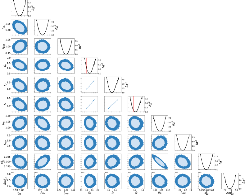
Figure 1: Constraints from our global analysis on the solar neutrino fluxes for the analysis with luminosity constraint and fixed ratios of the CNO fluxes (see Eq. (13)). Each panel shows a two-dimensional projection of the allowed multidimensional parameter space after minimization with respect to the undisplayed parameters. The regions correspond to 90% and 99% CL (2 d.o.f.). The curves in the rightmost panels show the marginalized one-dimensional $\Delta\chi^{2}_{\text{wLC,CNO-Rfixed}}$ for each of the parameters.

We present first the results of our analysis with the luminosity constraint and the ratios of the CNO fluxes fixed by the relations in Eq. (12), so that altogether for this case we construct the $\chi^{2}$ function

$$\chi^{2}_{\text{wLC,CNO-Rfixed}}\equiv\chi^{2}_{\text{global}}(\vec{\omega}_{\text{osc}},\,\vec{\omega}_{\text{flux}}^{\text{CNO-Rfixed}})+\chi^{2}_{\text{pep/pp}}(f_{{\text{pp}}},\,f_{{\text{pep}}})+\chi^{2}_{\text{LC}}(\vec{\omega}_{\text{flux}}^{\text{CNO-Rfixed}})\,.$$ (13)

The results of this analysis are displayed in Fig. 1, where we show the two- and one-dimensional projections of $\Delta\chi^{2}_{\text{wLC,CNO-Rfixed}}$. From these results one reads that the ranges at $1\sigma$ (and at the $99\%$ CL in square brackets) for the two oscillation parameters are:

$$\Delta m^{2}_{21} =7.43_{-0.30}^{+0.30}\,[{}_{-0.49}^{+0.44}]\times 10^{-5}\text{eV}^{2}\,,$$ (14)

$$\sin^{2}\theta_{12} =0.300_{-0.017}^{+0.020}\,[{}_{-0.027}^{+0.031}]\,,$$

which are very similar to the results of NuFIT-5.2 nufit-5.2 with the expected slight enlargement of the allowed ranges. In other words, within the $3\nu$ scenario the data is precise enough to simultaneously constraint the oscillation parameters and the normalizations of the solar flux components without resulting into a substantial degradation of the former. As for the solar fluxes, the corresponding ranges read:

$$f_{{\text{pp}}} =0.9969_{-0.0039}^{+0.0041}\,[{}_{-0.0092}^{+0.0095}]\,,\qquad \Phi_{{\text{pp}}} =5.941_{-0.023}^{+0.024}\,[{}_{-0.055}^{+0.057}]\times 10^{10}~{}\text{cm}^{-2}~{}\text{s}^{-1}\,,$$ (15)

$$f_{{\mbox{}^{7}\text{Be}}} =1.019_{-0.017}^{+0.020}\,[{}_{-0.041}^{+0.047}]\,,\qquad \Phi_{{\mbox{}^{7}\text{Be}}} =4.93_{-0.08}^{+0.10}\,[{}_{-0.20}^{+0.23}]\times 10^{9}~{}\text{cm}^{-2}~{}\text{s}^{-1}\,,$$

$$f_{{\text{pep}}} =1.000_{-0.018}^{+0.016}\,[{}_{-0.042}^{+0.041}]\,,\qquad \Phi_{{\text{pep}}} =1.421_{-0.026}^{+0.023}\,[{}_{-0.060}^{+0.058}]\times 10^{8}~{}\text{cm}^{-2}~{}\text{s}^{-1}\,,$$

$$f_{{\mbox{}^{13}\text{N}}} =1.25_{-0.14}^{+0.17}\,[{}_{-0.40}^{+0.47}]\,,\qquad \Phi_{{\mbox{}^{13}\text{N}}} =3.48_{-0.40}^{+0.47}\,[{}_{-1.10}^{+1.30}]\times 10^{8}~{}\text{cm}^{-2}~{}\text{s}^{-1}\,,$$

$$f_{{\mbox{}^{15}\text{O}}} =1.22_{-0.14}^{+0.17}\,[{}_{-0.39}^{+0.46}]\qquad \Phi_{{\mbox{}^{15}\text{O}}} =2.53_{-0.29}^{+0.34}\,[{}_{-0.80}^{+0.94}]\times 10^{8}~{}\text{cm}^{-2}~{}\text{s}^{-1}\,,$$

$$f_{{\mbox{}^{17}\text{F}}} =1.03_{-0.20}^{+0.20}\,[{}_{-0.48}^{+0.47}]\,,\qquad \Phi_{{\mbox{}^{17}\text{F}}} =5.51_{-0.63}^{+0.75}\,[{}_{-1.75}^{+2.06}]\times 10^{7}~{}\text{cm}^{-2}~{}\text{s}^{-1}\,,$$

$$f_{{\mbox{}^{8}\text{B}}} =1.036_{-0.020}^{+0.020}\,[{}_{-0.048}^{+0.047}]\,,\qquad \Phi_{{\mbox{}^{8}\text{B}}} =5.20_{-0.10}^{+0.10}\,[{}_{-0.24}^{+0.24}]\times 10^{6}~{}\text{cm}^{-2}~{}\text{s}^{-1}\,,$$

$$f_{{\text{hep}}} =3.8_{-1.2}^{+1.1}\,[{}_{-2.7}^{+2.7}]\,,\qquad \Phi_{{\text{hep}}} =3.0_{-1.0}^{+0.9}\,[{}_{-2.1}^{+2.2}]\times 10^{4}~{}\text{cm}^{-2}~{}\text{s}^{-1}\,.$$

Notice that in Fig. 1 we separately plot the ranges for the three CNO flux normalization parameters, however they are fully correlated since their ratios are fixed, which explains the thin straight-line shape of the regions as seen in the three corresponding panels. Compared to the results from our previous analysis we now find that all the fluxes are clearly determined to be non-zero, while in Refs. Gonzalez-Garcia:2009dpj ; Bergstrom:2016cbh only an upper bound for the CNO fluxes was found. This is a direct consequence of the positive evidence of neutrinos produced in the CNO cycle provided by Borexino Phase-III spectral data, which is here confirmed in a fully consistent global analysis. We will discuss this point in more detail in Sec. 4. We also observe that the inclusion of the full statistics of Borexino has improved the determination of $f_{{\mbox{}^{7}\text{Be}}}$ by a factor $\mathcal{O}(3)$.

Figure 1 exhibits the expected correlation between the allowed ranges of the pp and pep fluxes, which is a consequence of the relation (8). This correlation is somewhat weaker than what observed in the corresponding analysis in Ref. Bergstrom:2016cbh because the spectral information from Borexino Phase-II and Phase-III provides now some independent information on $f_{{\text{pep}}}$. We also observe the presence of anticorrelation between the allowed ranges of the two most intense fluxes, pp and $\mbox{}^{7}\text{Be}$, as dictated by the luminosity constraint (see comparison with Fig. 2). Finally we notice that the allowed ranges of $f_{{\mbox{}^{7}\text{Be}}}$ and $f_{{\mbox{}^{8}\text{B}}}$ – the two most precise directly determined flux normalizations irrespective of the luminosity constraint (see Fig. 2) – are anticorrelated. This is a direct consequence of the different dependence of the survival probability with $\sin^{2}\theta_{12}$ in their respective energy ranges. $\mbox{}^{8}\text{B}$ neutrinos have energies of the order of several MeV for which the flavour transition occurs in the MSW regime and the survival probability $P_{ee}\propto\sin^{2}\theta_{12}$. Hence an increase in $\sin^{2}\theta_{12}$ must be compensated by a decrease of $f_{{\mbox{}^{8}\text{B}}}$ to get the correct number of events, which leads to the anticorrelation between the $\sin^{2}\theta_{12}$ and $f_{{\mbox{}^{8}\text{B}}}$ seen in the corresponding panel in Fig. 1. On the contrary, most $\mbox{}^{7}\text{Be}$ neutrinos have 0.86 MeV (some have 0.38 MeV) and for that energy the flavour transition occurs in the transition regime between MSW and vacuum average oscillations for which $P_{ee}$ decreases with $\sin^{2}\theta_{12}$. Hence the correlation between $\sin^{2}\theta_{12}$ and $f_{{\mbox{}^{7}\text{Be}}}$ seen in the corresponding panel. Altogether, this leads to the anticorrelation observed between $f_{{\mbox{}^{7}\text{Be}}}$ and $f_{{\mbox{}^{8}\text{B}}}$. This was already mildly present in the results in Ref. Bergstrom:2016cbh but it is now a more prominent feature because of the most precise determination of $f_{{\mbox{}^{7}\text{Be}}}$.

All these results imply the following share of the energy production between the pp-chain and the CNO-cycle

$$\frac{L_{\text{pp-chain}}}{L_{\odot}}=0.9919_{-0.0030}^{+0.0035}\,[{}_{-0.0077}^{+0.0082}]\quad\Longleftrightarrow\quad\frac{L_{\text{CNO}}}{L_{\odot}}=0.0079_{-0.0011}^{+0.0009}\,[{}_{-0.0026}^{+0.0028}]$$ (16)

in perfect agreement with the SSMs which predict $L_{\text{CNO}}\big{/}L_{\odot}\leq 1\%$ at the $3\sigma$ level. Once again we notice that in the present analysis the evidence for $L_{\text{CNO}}\neq 0$ clearly stands well above 99% CL.

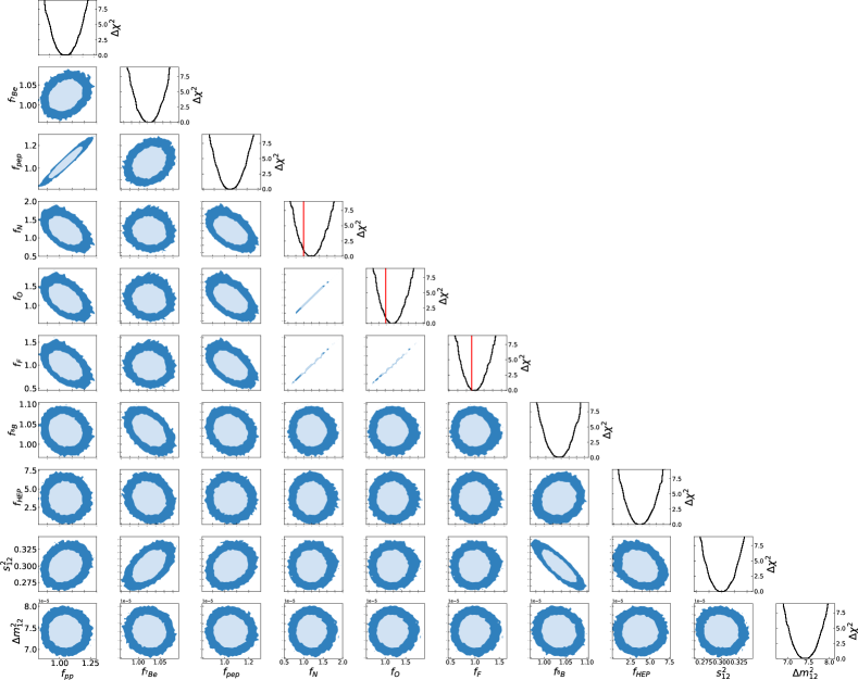
Figure 2: Same as Fig. 1 but without imposing the luminosity constraint (see Eq. (17)).

We next show in Fig. 2 the results of the analysis performed without imposing the luminosity constraint – but still with the ratios of the CNO fluxes fixed by the relations in Eq. (12) – for which we employ

$$\chi^{2}_{\text{woLC,CNO-Rfixed}}\equiv\chi^{2}_{\text{global}}(\vec{\omega}_{\text{osc}},\,\vec{\omega}_{\text{flux}}^{\text{CNO-Rfixed}})+\chi^{2}_{\text{pep/pp}}(f_{{\text{pp}}},\,f_{{\text{pep}}})\,.$$ (17)

The allowed ranges for the fluxes in this case are:

$$f_{{\text{pp}}} =1.038_{-0.066}^{+0.076}\,[{}_{-0.16}^{+0.18}]\,,\qquad \Phi_{{\text{pp}}} =6.19_{-0.39}^{+0.45}\,[{}_{-1.0}^{+1.1}]\times 10^{10}~{}\text{cm}^{-2}~{}\text{s}^{-1}\,,$$ (18)

$$f_{{\mbox{}^{7}\text{Be}}} =1.022_{-0.018}^{+0.022}\,[{}_{-0.042}^{+0.051}]\,,\qquad \Phi_{{\mbox{}^{7}\text{Be}}} =4.95_{-0.089}^{+0.11}\,[{}_{-0.22}^{+0.25}]\times 10^{9}~{}\text{cm}^{-2}~{}\text{s}^{-1}\,,$$

$$f_{{\text{pep}}} =1.039_{-0.065}^{+0.082}\,[{}_{-0.16}^{+0.19}]\,,\qquad \Phi_{{\text{pep}}} =1.48_{-0.09}^{+0.11}\,[{}_{-0.22}^{+0.26}]\times 10^{8}~{}\text{cm}^{-2}~{}\text{s}^{-1}\,,$$

$$f_{{\mbox{}^{13}\text{N}}} =1.16_{-0.19}^{+0.19}\,[{}_{-0.45}^{+0.50}]\,,\qquad \Phi_{{\mbox{}^{13}\text{N}}} =3.32_{-0.54}^{+0.53}\,[{}_{-1.24}^{+1.40}]\times 10^{8}~{}\text{cm}^{-2}~{}\text{s}^{-1}\,,$$

$$f_{{\mbox{}^{15}\text{O}}} =1.16_{-0.19}^{+0.19}\,[{}_{-0.44}^{+0.49}]\qquad \Phi_{{\mbox{}^{15}\text{O}}} =2.41_{-0.39}^{+0.38}\,[{}_{-0.90}^{+1.02}]\times 10^{8}~{}\text{cm}^{-2}~{}\text{s}^{-1}\,,$$

$$f_{{\mbox{}^{17}\text{F}}} =1.01_{-0.16}^{+0.16}\,[{}_{-0.38}^{+0.45}]\,,\qquad \Phi_{{\mbox{}^{17}\text{F}}} =5.25_{-0.85}^{+0.84}\,[{}_{-1.97}^{+2.21}]\times 10^{6}~{}\text{cm}^{-2}~{}\text{s}^{-1}\,,$$

$$f_{{\mbox{}^{8}\text{B}}} =1.034_{-0.021}^{+0.020}\,[{}_{-0.051}^{+0.052}]\,,\qquad \Phi_{{\mbox{}^{8}\text{B}}} =5.192_{-0.11}^{+0.10}\,[{}_{-0.26}^{+0.26}]\times 10^{6}~{}\text{cm}^{-2}~{}\text{s}^{-1}\,,$$

$$f_{{\text{hep}}} =3.6_{-1.1}^{+1.2}\,[{}_{-2.6}^{+3.0}]\,,\qquad \Phi_{{\text{hep}}} =2.9_{-0.9}^{+1.0}\,[{}_{-2.1}^{+2.4}]\times 10^{4}~{}\text{cm}^{-2}~{}\text{s}^{-1}\,.$$

As expected, the pp flux is the most affected by the release of the luminosity constraint as it is this reaction which gives the largest contribution to the solar energy production and therefore its associated neutrino flux is the one more strongly bounded when imposing the luminosity constraint. The pep flux is also affected due to its strong correlation with the pp flux, Eq. (8). The CNO fluxes are mildly affected in an indirect way due to the modified contribution of the pep fluxes to the Borexino spectra.

Thus we find that the energy production in the pp-chain and the CNO-cycle without imposing the luminosity constraint are given by:

$$\frac{L_{\text{pp-chain}}}{L_{\odot}}=1.030_{-0.061}^{+0.070}\,[{}_{-0.15}^{+0.17}]\qquad\text{and}\qquad\frac{L_{\text{CNO}}}{L_{\odot}}=0.0075_{-0.0013}^{+0.0013}\,[{}_{-0.0029}^{+0.0030}]\,.$$ (19)

Comparing Eqs. (16) and (19) we see that while the amount of energy produced in the CNO cycle is about the same in both analysis, releasing the luminosity constraint allows for larger production of energy in the pp-chain. So in this case we find that the present value of the ratio of the neutrino-inferred solar luminosity, $L_{\odot}\text{(neutrino-inferred)}$, to the photon measured luminosity $L_{\odot}$ is:

$$\frac{L_{\odot}\text{(neutrino-inferred)}}{L_{\odot}}=1.038_{-0.060}^{+0.069}\,[{}_{-0.15}^{+0.17}]\,.$$ (20)

The neutrino-inferred luminosity is in good agreement with the one measured in photons, with a $1\sigma$ uncertainty of $\sim 6\%$. This represents only a very small variation with respect to the previous best determination Bergstrom:2016cbh . Such result is expected because the determination of the pp flux, which, as mentioned above gives the largest contribution to the neutrino-inferred solar luminosity, has not improved sensibly with the inclusion of the full statistics of the phases II and III of Borexino.

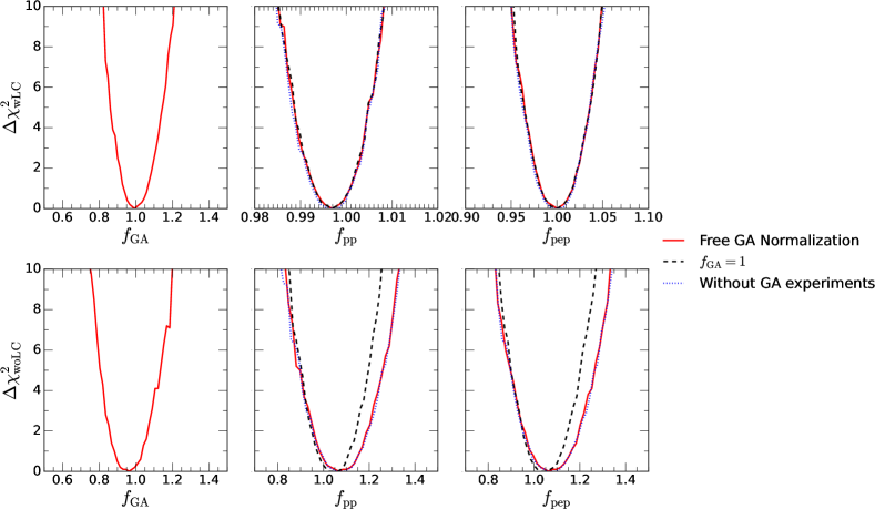
Figure 3: Dependence of the determination of the pp and pep fluxes on the assumptions about the Gallium experiments included in the analysis. The upper (lower) panels show the results of different variants of the analysis <<CNO-Rfixed>> with (without) luminosity constraint. See text for details.

We finish this section by discussing the role of the Gallium experiments in these results with the aim of addressing the possible impact of the Gallium anomaly Laveder:2007zz ; Acero:2007su ; Giunti:2010zu . As described in the introduction, this anomaly consists in a deficit of the event rate observed in Gallium source experiments with respect to the expectation, which represents an obvious puzzle for the interpretation of the results of the solar neutrino Gallium measurements. In this work we assume the well established standard $3\nu$ oscillation scenario and in this context the attempts at explanation (or at least alleviation) of the anomaly invoke the uncertainties of the capture cross section Berryman:2021yan ; Giunti:2022xat ; Elliott:2023xkb . Thus the open question posed by the Gallium anomaly is the possible impact of such modification of the cross section in the results of our fit.

In order to quantify this we performed two additional variants of our analysis. In the first one we introduce an additional parameter, $f_{\text{GA}}$, which multiplies the predicted event rates from all solar fluxes in the Gallium experiments. This parameter is left free to vary in the fits and would mimic an energy independent modification of the capture cross section (or equivalently of the detection efficiency). In the second variant we simply drop Gallium experiments from our global fit.

The results of these explorations are shown in Fig. 3 where we plot the most relevant marginalized one-dimensional projections of $\Delta\chi^{2}$ for these two variants. The upper (lower) panels correspond to analysis performed with (without) the luminosity constraint. The left panel shows the projection over the normalization parameter $f_{\text{GA}}$ obtained in the variant of the analysis which makes use of this parameter. As seen from the figure, the results of the fit favour $f_{\text{GA}}$ close to one, or, in other words, the global analysis of the solar experiments do not support a modification of the neutrino capture cross section in Gallium (or any other effect inducing an energy-independent reduction of the detection efficiency in the Gallium experiments). This is so because, within the $3\nu$ oscillation scenario, the global fit implies a rate of pp and $\mbox{}^{7}\text{Be}$ neutrinos in the Gallium experiment which is in good agreement with the luminosity constraint as well as with the rates observed in Borexino.

On the central and right panel of the figure we show the corresponding modification of marginalized one-dimensional projections of $\Delta\chi^{2}$ on the pp and pep flux normalizations which are those mostly affected in these variants. For the sake of comparison, in the upper and lower panels we also plot the results for the $f_{\text{GA}}=1$ analysis (also visible in the corresponding windows in Figs. 1 and 2, respectively). The figure illustrates that once the luminosity constraint is imposed, the determination of the solar fluxes is totally unaffected by the assumptions about the capture rate in Gallium. As seen in the lower panels, even without the luminosity constraint the impact on the pp and pep determination is marginal, which emphasizes the robustness of the flux determination in Eqs. (15) and (18). This is the case thanks to the independent precise determination of the pp flux in the phases I and II in Borexino. Furthermore, the small modification is the same irrespective of whether the Gallium capture rate is left free or completely removed from the analysis; this is due to the lack of spectral and day-night capabilities in Gallium experiments, which prevents them from providing further information beyond the overall normalization scale of the signal.

4 Examination of the determination of the CNO fluxes

As mentioned above, one of the most important developments in the experimental determination of the solar neutrino fluxes in the last years have been the evidence of neutrinos produced in the CNO cycle reported by Borexino BOREXINO:2020aww ; BOREXINO:2022abl ; Borexino:2023puw . The detection was made possible thanks to a novel method to constrain the rate of the $\mbox{}^{210}\text{Bi}$ background. In Ref. BOREXINO:2020aww , using a partial sample of their Phase-III data, the collaboration found a $5.1\sigma$ significance of the CNO flux observation, which increased to $7\sigma$ with the full Phase-III statistics BOREXINO:2022abl , and to about $8\sigma$ when combined with the CID method Borexino:2023puw . See appendix A for details.

Key ingredients in the analysis performed by the collaboration in Refs. BOREXINO:2020aww ; BOREXINO:2022abl ; Borexino:2023puw (and therefore in the derivation of these results) are the assumptions about the relative contribution of the three reactions producing neutrinos in the CNO cycle, as well as those about other solar fluxes in the same energy range, in particular the pep neutrinos. In a nutshell, as mentioned above, the collaboration assumes a common shift of the normalization of the CNO fluxes with respect to that of the SSM, and it is the evidence of a non-zero value of such normalization which is quantified in Refs. BOREXINO:2020aww ; BOREXINO:2022abl ; Borexino:2023puw . In what respects the rate from the pep flux, the SSM expectation was assumed because the Phase-III data by itself does not allow to constraint simultaneously the CNO and pep flux normalizations.

In this respect, the global analysis presented in the previous section are performed under the same paradigm of a common shift normalization of the CNO fluxes, but being global, the pep flux normalization is also simultaneously fitted. For the sake of comparison we reproduce in Fig. 4 the projection of the marginalized $\Delta\chi^{2}_{\text{wLC,CNO-Rfixed}}$ (13) and $\Delta\chi^{2}_{\text{woLC,CNO-Rfixed}}$ (13) on the normalization parameters for the three CNO fluxes. For convenience we also show the projections as a function of the total neutrino flux produced in the CNO cycle. As seen in the figure the results of the analysis (either with or without luminosity constraint) yield a value of $\Delta\chi^{2}$ well beyond $3\sigma$ for $\Phi_{{\text{CNO}}}=0$. A dedicated run for this no-CNO scenario case gives $\Delta\chi^{2}=54$ ($33$) for the analysis with (without) luminosity constraints, and it is therefore excluded at $7.3\sigma$ ($5.7\sigma$) CL.

In order to study the dependence of the results on the assumption of a unique common shift of the normalization of three CNO fluxes we explored the possibility of making a global analysis in which the three normalization parameters are varied independently. As mentioned above, a priori the three normalizations only have to be subject to a minimum set of consistency relations in Eqs. (10) and (11). However, as discussed in detail in Sec. A.2, the background model in Refs. BOREXINO:2020aww ; BOREXINO:2022abl ; Borexino:2023puw only assumes an upper bound on the amount of $\mbox{}^{210}\text{Bi}$ and cannot be reliably employed to such general analysis because of the larger degeneracy between the $\mbox{}^{210}\text{Bi}$ background and the $\mbox{}^{13}\text{N}$ flux spectra.

With this limitation in mind, we proceed to perform two alternative analysis (with and without imposing the luminosity constraints) in which the normalization of the three CNO fluxes are left free to vary independently but with ratios constrained within a range broad enough to generously account for all variants of the B23 SSM, but not to extend into regions of the parameter space where the assumptions on the background model may not be applicable. Conservatively neglecting correlations between their theoretical uncertainties, the neutrino fluxes of SSMs presented in Ref. Magg:2022rxb and available publicly through a public repository B23Fluxes verify

$$\frac{f_{{\mbox{}^{15}\text{O}}}}{f_{{\mbox{}^{13}\text{N}}}}=\begin{cases}1.00\,(1\pm 0.24)\\ 0.95\,(1\pm 0.22)\\ 0.96\,(1\pm 0.21)\\ 1.01\,(1\pm 0.23)\\ 1.00\,(1\pm 0.23)\end{cases}\qquad\frac{f_{{\mbox{}^{17}\text{F}}}}{f_{{\mbox{}^{13}\text{N}}}}=\begin{cases}1.00\,(1\pm 0.25)&\text{B23-GS98}\\ 0.84\,(1\pm 0.23)&\text{B23-AGSS09-met}\\ 0.80\,(1\pm 0.20)&\text{B23-AAG21}\\ 0.79\,(1\pm 0.22)&\text{B23-MB22-met}\\ 0.79\,(1\pm 0.22)&\text{B23-MB22-phot}\end{cases}$$ (21)

Thus in these analyses, here onward labeled <<CNO-Rbound>>, we introduce two pulls $\xi_{1}$ and $\xi_{2}$ for these two ratios. Notice, however, that we could have equally defined the priors with respect to the reciprocal of the ratios in Eq. (21). Hence, in order to avoid a bias towards larger fluxes in the numerator versus the denominator introduced by either choice, we resort instead to logarithmic priors for the ratios:

$$\vec{\omega}_{\text{flux}}^{\text{CNO-Rbound}}\equiv(f_{{\text{pp}}},\;f_{{\mbox{}^{7}\text{Be}}},\;f_{{\text{pep}}},\;f_{{\mbox{}^{13}\text{N}}},\\ f_{{\mbox{}^{15}\text{O}}}=0.98\,\exp(\xi_{1})\,f_{{\mbox{}^{13}\text{N}}},\;f_{{\mbox{}^{17}\text{F}}}=0.85\,\exp(\xi_{2})\,f_{{\mbox{}^{13}\text{N}}},\;f_{{\mbox{}^{8}\text{B}}},\;f_{{\text{hep}}})$$ (22)

and add two Gaussian penalty factors for these pulls, so that the corresponding $\chi^{2}$ function without the luminosity constraint is:

$$\chi^{2}_{\text{woLC,CNO-Rbound}}\equiv\chi^{2}_{\text{global}}(\vec{\omega}_{\text{osc}},\,\vec{\omega}_{\text{flux}}^{\text{CNO-Rbound}})+\chi^{2}_{\text{pep/pp}}(f_{{\text{pp}}},\,f_{{\text{pep}}})+\frac{\xi_{1}^{2}}{\sigma_{\xi_{1}}^{2}}+\frac{\xi_{2}^{2}}{\sigma_{\xi_{2}}^{2}}$$ (23)

with $\sigma_{\xi_{1}}=0.26$ and $\sigma_{\xi_{2}}=0.48$, chosen to cover the ranges in Eq. (21). In addition $f_{{\mbox{}^{13}\text{N}}}$, $f_{{\mbox{}^{15}\text{O}}}$, and $f_{{\mbox{}^{17}\text{F}}}$ are required to verify the consistency relations in Eqs. (10) and (11). The $\chi^{2}$ function with the luminosity constraint is obtained by further including the $\chi^{2}_{\text{LC}}$ prior of Eq. (5):

$$\chi^{2}_{\text{wLC,CNO-Rbound}}\equiv\chi^{2}_{\text{woLC,CNO-Rbound}}+\chi^{2}_{\text{LC}}(\vec{\omega}_{\text{flux}}^{\text{CNO-Rbound}})\,.$$ (24)

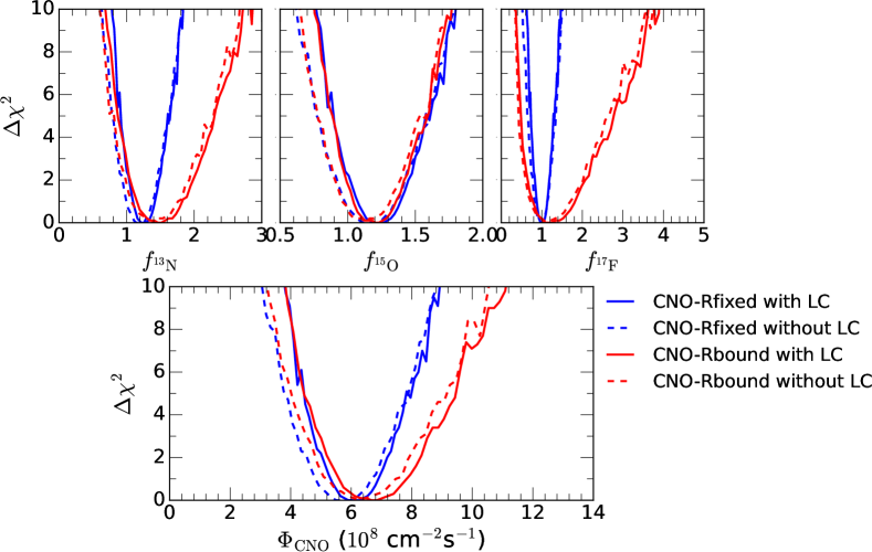
Figure 4: One dimensional projections of the global $\Delta\chi^{2}$ of the for the three neutrino fluxes produced in the CNO-cycle for different assumptions as labeled in the figure. See text for details.

We plot in Fig. 4 the projection of the marginalized $\Delta\chi^{2}_{\text{wLC,CNO-Rbound}}$ (24) and $\Delta\chi^{2}_{\text{woLC,CNO-Rbound}}$ (24) on the normalization parameters for the three CNO fluxes as well as on the total neutrino flux produced in the CNO cycle. As seen in the figure, allowing for the ratios of the CNO normalizations to vary within the intervals (21) has little impact on the allowed range of the $\mbox{}^{15}\text{O}$ flux and on the lower limit of the $\mbox{}^{13}\text{N}$ and $\mbox{}^{17}\text{F}$ fluxes. As a consequence, the CL at which the no-CNO scenario can be ruled out is unaffected. On the contrary, we see in Fig. 4 that the upper bound on the $\mbox{}^{13}\text{N}$ and $\mbox{}^{17}\text{F}$ fluxes, and therefore of the total neutrino flux produced in the CNO-cycle, is relaxed. This is a consequence of the strong degeneracy between the spectrum of events from these fluxes and those from the $\mbox{}^{210}\text{Bi}$ background mentioned above, see Fig. 10 and discussion in Sec. A.2. Conversely the fact that the range of the $\mbox{}^{15}\text{O}$ flux is robust under the relaxation of the constraints on the CNO flux ratios, means that the high statistics spectral data of the Phase-III of Borexino holds the potential to differentiate the event rates from $\mbox{}^{15}\text{O}$ $\nu$’s from those from $\mbox{}^{13}\text{N}$ and $\mbox{}^{17}\text{F}$ $\nu$’s. The reliable quantification of this possibility, however, requires the knowledge of the minimum allowed value of the $\mbox{}^{210}\text{Bi}$ background which so far has not been presented by the collaboration.

So, let us emphasize that our <<CNO-Rbound>> analysis have been performed with the aim of testing the effect of relaxing the severe constrains on the CNO fluxes in the studies of the Borexino collaboration. Our conclusion is that the statistical significance of the evidence of detection of events produced by neutrinos from the CNO-cycle is affected very little by the relaxation of the constraint on their relative ratios. However, their allowed range is, and this can have an impact when confronting the results of the fit with the predictions of the SSM as we discuss next.

5 Comparison with Standard Solar Models

Next we compare the results of our determination of the solar fluxes with the expectations from the five B23 solar models: SSMs computed with the abundances compiled in table 5 of Magg:2022rxb based on the photospheric and meteoritic solar mixtures (MB22-phot and MB22-met models, respectively), and with the Asplund2021 (AAG21), the meteoritic scale from Asplund2009 (AGSS09-met), and Grevesse1998 (GS98) compositions. We use both MB22-phot and MB22-met for completeness, although the abundances are very similar in both scales, as clearly reflected by the results in this section. A similar agreement would be found using both the meteoritic and photospheric scales from AAG21, and therefore we use only one scale in this case.

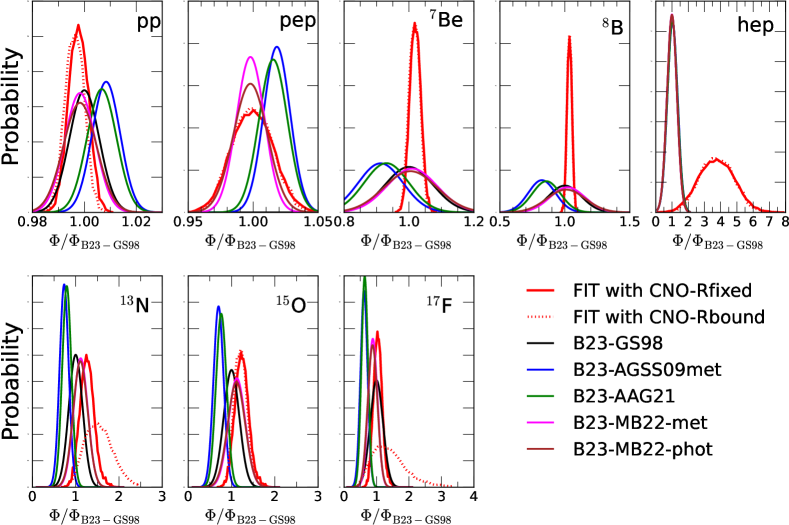
Figure 5: Marginalized one-dimensional probability distributions for the best determined solar fluxes in our analysis as compared to the predictions for the five SSMs in Ref. Magg:2022rxb ; B23Fluxes .

SSMs predict that nuclear energy accounts for all the solar luminosity (barred about a few parts in $10^{4}$ that are of gravothermal origin) so for all practical matters the neutrino fluxes predicted by SSMs satisfy the luminosity constraint. Therefore we compare the expectations of the various SSM models with the results of our analysis performed with such constraint. In what respects the assumptions on the CNO fluxes, in order to explore the dependence of our conclusions on the specific choice of flux ratios we quantify the results obtained in both the <<FIT=CNO-Rfixed>> analysis (with $\chi^{2}_{\text{FIT}}$ in Eq. (13)) and the <<FIT=CNO-Rbounded>> one (with $\chi^{2}_{\text{FIT}}$ in Eq. (24)). For illustration we plot in Fig. 5 the marginalized one-dimensional probability distributions for the best determined solar fluxes in such two cases as compared to the predictions for the five B23 SSMs. The probability distributions for our fits are obtained from the one-dimensional marginalized $\Delta\chi^{2}_{\text{FIT}}(f_{i})$ of the corresponding analysis as $P_{\text{FIT}}(f_{i})\propto\exp[-\Delta\chi^{2}_{\text{FIT}}(f_{i})/2]$ normalized to unity. To construct the analogous distributions for each of the SSMs we use the predictions $\langle f_{i}^{\text{SSM}}\rangle$ for the fluxes, the relative uncertainties $\sigma_{i}^{\text{SSM}}$ and their correlations $\rho_{ij}^{\text{SSM}}$ as obtained from Refs. B23Fluxes , and also assume gaussianity so to build the corresponding $\chi^{2}_{\text{SSM}}(\vec{\omega}_{\text{flux}})$

$$\chi^{2}_{\text{SSM}}(\vec{\omega}_{\text{flux}})=\sum_{i,j}(f_{i}-f_{i}^{\text{SSM}})C^{-1}_{ij}(f_{i}-f_{i}^{\text{SSM}})\quad\text{with}\quad C_{ab}=\sigma_{a}^{\text{SSM}}\sigma_{b}^{\text{SSM}}\rho_{ab}\,,$$ (25)

from which it is trivial to obtain the marginalized one-dimensional $\Delta\chi^{2}_{\text{SSM}}(f_{i})$ and construct the probability $P_{\text{SSM}}(f_{i})\propto\exp[-\Delta\chi^{2}_{\text{SSM}}(f_{i})/2]$.

In the frequentist statistical approach, quantitative comparison of a model prediction for a set of fluxes with the results from the data analysis can be obtained using the parameter goodness of fit (PG) criterion introduced in Ref. Maltoni:2003cu , by comparing the minimum value of $\chi^{2}$ function for the analysis of the data with that obtained for the same analysis adding the prior imposed by the model. Thus, following Ref. Maltoni:2003cu , we construct the test statistics

$$\Delta\chi^{2}_{\text{FIT,SSM,SET}}=\left.\big{[}\chi^{2}_{\text{FIT}}(\vec{\omega}_{\text{osc}},\,\vec{\omega}_{\text{flux}}^{\text{FIT}})+\chi^{2}_{\text{SSM,SET}}(\vec{\omega}_{\text{flux}}^{\text{FIT}})\big{]}\right|_{\text{min}}\\ -\left.\chi^{2}_{\text{FIT}}(\vec{\omega}_{\text{osc}},\,\vec{\omega}_{\text{flux}}^{\text{FIT}})\right|_{\text{min}}-\left.\chi^{2}_{\text{SSM,SET}}(\vec{\omega}_{\text{flux}}^{\text{FIT}})\right|_{\text{min}}$$ (26)

where $\chi^{2}_{\text{SSM,SET}}(\vec{\omega}_{\text{flux}})$ is obtained as Eq. (25) with $i,j$ (and $a,b$) fluxes restricted to a specific subset as specified by “SET”. The minimization of each of the terms in Eq. (26) is performed independently in the corresponding parameter space. $\Delta\chi^{2}_{\text{FIT,SSM,SET}}$ follows a $\chi^{2}$ distribution with $n$ degrees of freedom, which, in the present case, coincides with the number of free parameters in common between $\chi^{2}_{\text{FIT}}(\vec{\omega}_{\text{osc}},\,\vec{\omega}_{\text{flux}}^{\text{FIT}})$ and $\chi^{2}_{\text{SSM,SET}}(\vec{\omega}_{\text{flux}}^{\text{FIT}})$. Notice that, by construction, the result of the test depends on the number of fluxes to be compared, i.e., on the fluxes in “SET”, both because of the actual comparison between the measured and predicted values for those specific fluxes, and because of the change in $n$ with which the $p$-value of the model is to be computed. This is illustrated in Table 2 where we list the values of $\Delta\chi^{2}_{\text{FIT,SSM,SET}}$ for different choices of “SET” which we have labeled as:

SET constrained fluxes

FULL ($$f_{{\text{pp}}}$$, ,  , , , , , )

Be+B+CNO (, , , , )

CNO (, , )

(27)

FIT	B23-SSM	FULL			Be+B+CNO			CNO
CNO-Rfixed		n=6			n=3			n=1
		$\Delta\chi^{2}$	$p_{\text{GF}}$	CL [$\sigma$]	$\Delta\chi^{2}$	$p_{\text{GF}}$	CL [$\sigma$]	$\Delta\chi^{2}$	$p_{\text{GF}}$	CL [$\sigma$]
	AGSS09-met	14.5	0.024	2.3	9.8	0.020	2.30	7.2	0.0073	2.7
	GS98	08.1	0.240	1.2	3.0	0.390	0.86	2.4	0.1200	1.5
	AAG21	12.5	0.052	1.9	7.8	0.050	2.00	6.2	0.0130	2.5
	MB22-met/phot	07.1	0.310	1.0	2.2	0.530	0.62	2.0	0.1600	1.4
CNO-Rbound		n=8			n=5			n=3
		$\Delta\chi^{2}$	$p_{\text{GF}}$	CL [$\sigma$]	$\Delta\chi^{2}$	$p_{\text{GF}}$	CL [$\sigma$]	$\Delta\chi^{2}$	$p_{\text{GF}}$	CL [$\sigma$]
	AGSS09-met	14.1	0.079	1.80	9.3	0.098	1.70	7.2	0.066	1.80
	GS98	06.7	0.570	0.57	1.7	0.880	0.14	1.6	0.660	0.44
	AAG21	11.7	0.160	1.40	6.8	0.240	1.20	5.7	0.130	1.50
	MB22-met/phot	05.9	0.660	0.44	1.1	0.950	0.06	1.0	0.800	0.25

Table 2: Results of the PG test for the different models and data samples considered. Within the given accuracy the results for MB22-met and MB22-phot models are the same.

Upon analyzing the data in the Table 2, it becomes evident that the B23-MB22 models (both the meteoritic and photospheric variations) exhibit a significantly higher level of compatibility with the observed data, even slightly better the B23-GS98 model. On the contrary the B23-AGSS09met and B23-AAG21 models exhibits a lower level of compatibility with observations, with B23-AAG21 model slightly better aligned with the data. Maximum discrimination is provided by comparing mainly the CNO fluxes for which the prediction of both models is mostly different. On the other hand, including all the fluxes from the pp-chain in the comparison tends to dilute the discriminating power of the test. The table also illustrates how allowing for the three CNO fluxes normalizations to vary in the fit tends to relax the CL at which the models are compatible with the observations.

Let us remember that our previously determined fluxes in Ref Bergstrom:2016cbh when confronted with the GS98 and AGSS09 models of the time Serenelli:2011py showed absolutely no preference for either model. This was driven by the fact that the most precisely measured $\mbox{}^{8}\text{B}$ flux (and also of $\mbox{}^{7}\text{Be}$) laid right in the middle of the prediction of both models. The new B16-GS98 model in Ref. Vinyoles:2016djt predicted a slightly lower value for $\mbox{}^{8}\text{B}$ flux in slightly better agreement with the extracted fluxes of Ref Bergstrom:2016cbh , but the conclusion was still that there was no significant preference for either model. Compared to those results, both the most precisely determined $\mbox{}^{7}\text{Be}$ flux and, most importantly, the newly observed rate of CNO events in Borexino have consistently moved towards the prediction of the models with higher metallicity abundances.

Let us finish commenting on the relative weight of the experimental precision versus the theoretical model uncertainties in the results in Table 2. To this end one can envision an ideal experiment which measures $f_{i}$ to match precisely the values predicted by one of the models with infinite accuracy. Assuming the measurements to coincide with the predictions of B23-GS98, one gets $\Delta\chi^{2}_{\text{SSM,SET}}=17.1$ and $16.7$ for SSM=B23-AGSS09-met and SSM=B23-AAG21 with SET=FULL, which means that the maximum CL at which these two SSM can be disfavoured is $2.2\sigma$ and $2.1\sigma$. Choosing instead SET=CNO these numbers become $\Delta\chi^{2}_{\text{SSM,SET}}=15.0$ and $14.1$ for SSM=B23-AGSS09-met and SSM=B23-AAG21, respectively, corresponding to a $3.1\sigma$ and $3.0\sigma$ maximum rejection. This stresses the importance of reducing the uncertainties in the model predictions to boost the discrimination between the models.

6 Summary

In this work we have updated our former determination of solar neutrino fluxes from neutrino data as presented in Refs. Gonzalez-Garcia:2009dpj ; Bergstrom:2016cbh , by incorporating into the analysis the latest results from both solar and non-solar neutrino experiments. In particular this includes the full data from the three phases of the Borexino experiments which have provided us with the first direct evidence of neutrinos produced in the CNO-cycle.

We have derived the best neutrino oscillation parameters and solar fluxes constraints using a frequentist analysis with and without imposing nuclear physics as the only source of energy generation (luminosity constraint). Compared to the results from previous analysis we find that the determination of the $\mbox{}^{7}\text{Be}$ flux has improved by a factor $\mathcal{O}(3)$, but most importantly we now find that the three fluxes produced in the CNO-cycle are clearly determined to be non-zero, with $1\sigma$ precision ranges between 20% to $\sim 100\%$ depending on the assumptions in the analysis about their relative normalization. Conversely, in Refs. Gonzalez-Garcia:2009dpj ; Bergstrom:2016cbh only an upper bound for the CNO fluxes was found. This also implies that it is solidly established that at 99% CL the solar energy produced in the CNO-cycle is between $0.46\%$ and $1.05\%$ of the total solar luminosity.

The observation of the CNO neutrinos is also paramount to discriminate among the different versions of the SSMs built with different inputs for the solar abundances, since the CNO fluxes are the most sensitive to the solar composition. In this work we confront for the first time the neutrino fluxes determined on a purely experimental basis with the predictions of the latest generation of SSM obtained in Ref. Magg:2022rxb ; B23Fluxes . Our results show that the SSMs built incorporating lower metallicities are less compatible with the solar neutrino observations.

Appendix A Details of Borexino analysis

A detailed description of our analysis of the full spectrum of the Phase-I Bellini:2011rx ; Bellini:2008mr and Phase-II Borexino:2017rsf of Borexino can be found in Ref. Gonzalez-Garcia:2009dpj and Ref. Coloma:2022umy respectively. Here we document the details of our analysis of the Borexino Phase-III data collected from January 2017 to October 2021, corresponding to a total exposure of $\text{1431.6 days}\times\text{71.3 tons}$, which we perform following closely the details presented by the collaboration in Refs. BOREXINO:2020aww ; BOREXINO:2022abl .

A.1 Analysis of Borexino Phase-III spectrum

In our fit we use the Borexino spectral data as a function of the detected hits ($N_{h}$) on the detector photomultipliers (including multiple hits on the same photomultiplier) as estimator of the recoil energy of the electron. At it was the case in Phase-II, Borexino divide their Phase-III data in two samples: one enriched (tagged) and one depleted (subtracted) in the $\mbox{}^{11}\text{C}$ events. The tagged sample picks up about $36\%$ of the solar neutrino events, while the subtracted sample accounts for the remaining $64\%$. In what follows we denote by $s=$”tagged” or $s=$”subtracted” each of the two samples. The data and best fit components for the spectrum of the subtracted sample are shown in Fig. 2(a) of Ref. BOREXINO:2022abl . The data points for this sample can also be found in the data release material in Ref. borexdata . The corresponding information for the tagged sample was kindly provided to us by the Borexino collaboration borextag .

The number of expected events $T^{0}_{s,i}$ in some bin $i$ of data sample $s$ is the sum of the neutrino-induced signal and the background contributions. The main backgrounds come from radioactive isotopes in the scintillator $\mbox{}^{11}\text{C}$, $\mbox{}^{210}\text{Bi}$, $\mbox{}^{10}\text{C}$, $\mbox{}^{210}\text{Po}$ and $\mbox{}^{85}\text{Kr}$. The collaboration identifies one additional background due to residual external backgrounds. With this

$$T^{0}_{s,i}=\sum_{f}S^{f}_{s,i}+\sum_{c}B^{c}_{s,i}$$ (28)

where the index $f\in\{{\mbox{}^{7}\text{Be}},{\text{pep}},{\mbox{}^{13}\text{N}},{\mbox{}^{15}\text{0}},{\mbox{}^{17}\text{F}},{\mbox{}^{8}\text{B}}\}$ runs over the solar fluxes which contribute in the Borexino-III energy range (see Fig. 8), while the index $c\in\{{\mbox{}^{11}\text{C}},\allowbreak{\mbox{}^{210}\text{Po}},\allowbreak{\mbox{}^{210}\text{Bi}},\allowbreak{\mbox{}^{85}\text{Kr}},\allowbreak{\mbox{}^{10}\text{C}},\allowbreak{\text{ext}}\}$ runs over the background components.

We compute the solar neutrino signal from flux $f$ in bin $i$, $S^{f}_{s,i}$, as

$$S^{f}_{s,i}=\int_{N_{h,\text{min}}^{i}}^{N_{h,\text{max}}^{i}}\int\frac{\mathrm{d}S^{f}_{s}}{\mathrm{d}T_{e}}(T_{e})\,\frac{\mathrm{d}\mathcal{R}}{\mathrm{d}N_{h}}(T_{e},N_{h})\,\mathrm{d}T_{e}\,\mathrm{d}N_{h}$$ (29)

where $\mathrm{d}S_{s}^{f}/\mathrm{d}T_{e}$ is the differential distribution of neutrino-induced events from flux $f$ to sample $s$ as a function of recoil energy of the scattered electrons ($T_{e}$)

$$\frac{\mathrm{d}S^{f}_{s}}{\mathrm{d}T_{e}}(T_{e})=\mathcal{F}_{s}\,\mathcal{N}_{\text{tgt}}\,\mathcal{T}_{\text{run}}\,\mathcal{E}_{\text{cut}}\sum_{\alpha}\int\frac{\mathrm{d}\phi^{f}_{\nu}}{\mathrm{d}E_{\nu}}\,P_{e\alpha}(E_{\nu})\,\frac{\mathrm{d}\sigma^{\text{det}}(\nu_{\alpha})}{\mathrm{d}T_{e}}\,\mathrm{d}E_{\nu}\,,$$ (30)

Here $\mathcal{F}_{s}=0.3572$ ($0.6359$) is the fraction for $s=\text{``tagged''}$ (“subtracted”) signal events, $\mathcal{N}_{\text{tgt}}$ is the number of $e^{-}$ targets (i.e., the total number of electrons inside the fiducial volume of the detector, corresponding to 71.3 ton of scintillator), $\mathcal{T}_{\text{run}}=1431.6$ days is the data taking time, $\mathcal{E}_{\text{cut}}=98.5\%$ is the overall efficiency (assumed to be the same as Phase-II), $P_{e\alpha}(E_{\nu})$ is the transition probability between the flavours $e$ and $\alpha$, and $\mathrm{d}\sigma^{\text{det}}(\nu_{\alpha})/\mathrm{d}T_{e}$ is the flavour dependent $\nu_{\alpha}-e^{-}$ elastic scattering detection cross section. The calculation of $P_{e\alpha}(E_{\nu})$ is based on a fully numerical approach which takes into account the specific distribution of the neutrino production point in the solar core for the various solar neutrino flux components as predicted by the SSMs; some technical details on our treatment of neutrino propagation in the solar matter can be found in Appendix A of Ref. Coloma:2022umy and in Sec. 2.4 of Ref. Maltoni:2023cpv . In addition Eq. (29) includes the energy resolution function $\mathrm{d}\mathcal{R}/\mathrm{d}T_{e}$ for the detector which gives the probability that an event with electron recoil energy $T_{e}$ yields an observed number of hits $N_{h}$. We assume it follows a Gaussian distribution

$$\frac{\mathrm{d}\mathcal{R}}{\mathrm{d}N_{h}}=\frac{1}{\sqrt{2\pi}\,\sigma_{h}(T_{e})}\exp\bigg{[}-\frac{1}{2}\bigg{(}\frac{N_{h}-\bar{N}_{h}(T_{e})}{\sigma_{h}(T_{e})}\bigg{)}^{2}\bigg{]}$$ (31)

where $\bar{N}_{h}$ is the expected value of $N_{h}$ for a given true recoil energy $T_{e}$. We determine $\bar{N}_{h}$ via the calibration procedure described in Ref. Coloma:2022umy , while $\sigma_{h}$ is slightly different from Borexino Phase-II analysis. Concretely, we derive a relation between $\bar{N}_{h}$ and $\sigma_{h}(\bar{N}_{h})$ which is

$$\sigma_{h}(\bar{N}_{h})=1.21974+1.60121\sqrt{\bar{N}_{h}}-0.14859\bar{N}_{h}.$$ (32)

In what respects the backgrounds, we have read the contribution $B^{c}_{s,i}$ for each component $c$ in each bin $i$ and for each data set $s$ from Fig. 2(a) of Ref. BOREXINO:2022abl as well as the plot provided to us by the collaboration borextag . These figures show the best-fit normalization of the different background components as obtained by the collaboration, and we take them as our nominal background predictions.

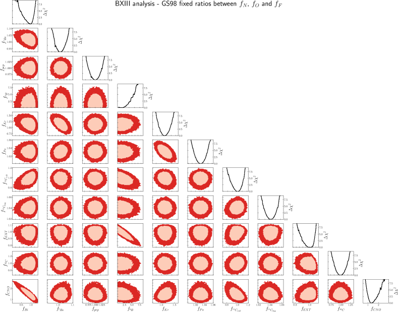
Figure 6: Constraints from our analysis of Borexino Phase-III spectra obtained with $\chi^{2}_{\text{BXIII,test}}$ in Eq. (36). Each panel shows a two-dimensional projection of the allowed multi-dimensional parameter space after minimization with respect to the undisplayed parameters. The regions correspond to 90% and 99% CL (2 d.o.f.). The curves in the right-most panels show the marginalized one-dimensional $\Delta\chi^{2}_{\text{BXIII,test}}$ for each of the parameters.

Our statistical analysis is based on the construction of a $\chi^{2}$ function built with the described experimental data, neutrino signal expectations and sources of backgrounds. Following Refs. BOREXINO:2020aww ; BOREXINO:2022abl we leave the normalization of all the backgrounds as free parameters with the exception of $\mbox{}^{210}\text{Bi}$. The treatment of this background is paramount to the positive evidence of CNO neutrinos. As described in BOREXINO:2020aww , the extraction of the CNO neutrino signal from the Borexino data faces two significant challenges: the resemblance between spectra of CNO-$\nu$ recoil electrons and the $\mbox{}^{210}\text{Bi}$ $\beta^{-}$ spectra, and their pronounced correlation with the pep-$\nu$ recoil energy spectrum. In order to surpass the first challenge, the collaboration restricted the rate of $\mbox{}^{210}\text{Bi}$ for which it sets and upper limit BOREXINO:2022abl :

$$R({\mbox{}^{210}\text{Bi}})\leq(10.8\pm 1.0)~{}\text{cpd}\big{/}\text{100\,t}\,,$$ (33)

while no constraint is imposed on its minimum value which is free to be as low as allowed by the fit (as long as it remains non-negative). We will go back to this point in Sec. A.2. In our analysis we implement this upper limit by constraining the corresponding normalization factor $f_{{\mbox{}^{210}\text{Bi}}}$ as

$$f_{{\mbox{}^{210}\text{Bi}}}\leq\bigg{(}1\pm\frac{1.0}{10.8}\bigg{)},$$ (34)

With this we construct the $\chi^{2}_{\text{BXIII}}$ as

$$\chi^{2}_{\text{BXIII}}=\sum_{s,i}2\bigg{[}T^{0}_{s,i}-O_{s,i}+O_{s,i}\log\bigg{(}\frac{O_{s,i}}{T^{0}_{s,i}}\bigg{)}\bigg{]}+\bigg{(}\frac{f_{{\mbox{}^{210}\text{Bi}}}-1}{\sigma_{{\mbox{}^{210}\text{Bi}}}}\bigg{)}^{2}\,\Theta(f_{{\mbox{}^{210}\text{Bi}}}-1)\,,$$ (35)

where $O_{s,i}$ is the observed number of events in bin $i$ of sample $s$, and $\sigma_{{\mbox{}^{210}\text{Bi}}}=1.0/10.8$, and $\Theta(x)$ is the Heaviside step function.

Constructed this way, $\chi^{2}_{\text{BXIII}}$ depends on 16 parameters: the 3 oscillation parameters ($\Delta m^{2}_{21}$, $\theta_{12}$, $\theta_{13}$), 6 solar flux normalizations ($f_{{\mbox{}^{7}\text{Be}}}$, $f_{{\text{pep}}}$, $f_{{\mbox{}^{13}\text{N}}}$, $f_{{\mbox{}^{15}\text{O}}}$, $f_{{\mbox{}^{17}\text{F}}}$, $f_{{\mbox{}^{8}\text{B}}}$) and 7 background normalizations ($f_{{\mbox{}^{210}\text{Po}}}$, $f_{{\mbox{}^{210}\text{Bi}}}$, $f_{{\mbox{}^{85}\text{Kr}}}$, $f_{{\mbox{}^{10}\text{C}}}$, $f_{\text{ext}}$ and two different factors $f_{{\mbox{}^{11}\text{C}}}^{\text{tag}}$ and $f_{{\mbox{}^{11}\text{C}}}^{\text{sub}}$ for the tagged and subtracted samples).

As a first validation of our $\chi^{2}$ function we perform an analysis focused at reproducing the results on the solar neutrino fluxes found by the Borexino collaboration in Ref. BOREXINO:2022abl , and in particular the positive evidence of CNO neutrinos. In this test fit we fix the three oscillation parameters to their best fit value ($\sin^{2}\theta_{13}=0.023$, $\sin^{2}\theta_{12}=0.307$, $\Delta m^{2}_{21}=7.5\times 10^{-5}$), and following the procedure of the collaboration we assume a common normalization factor for the three CNO fluxes with respect to the SSM ($f_{{\mbox{}^{13}\text{N}}}=f_{{\mbox{}^{15}\text{O}}}=f_{{\mbox{}^{17}\text{F}}}\equiv f_{{\text{CNO}}})$. Furthermore, in order to break the pronounced correlation with the pep-$\nu$ recoil energy spectrum mentioned above, the collaboration introduced a prior for the pep neutrino signal flux following the SSM. Thus we define

$$\chi^{2}_{\text{BXIII,test}}=\chi^{2}_{\text{BXIII}}+\bigg{(}\frac{f_{\text{pep}}-1}{\sigma_{{\text{pep}}}}\bigg{)}^{2}$$ (36)

with $\sigma_{{\text{pep}}}=0.04/2.74$ (for concreteness we choose the B16-GS98 model for this prior). The $\mbox{}^{7}\text{Be}$ and $\mbox{}^{8}\text{B}$ fluxes are left completely free.

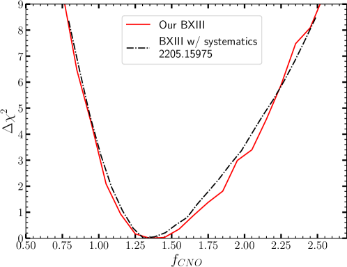
Figure 7: Dependence of $\Delta\chi^{2}$ of our fit to the Borexino Phase-III spectra on the common normalization of the CNO fluxes (red line). For comparison we plot (black dot-dashed line) the corresponding results in figure 2(b) of BOREXINO:2022abl for their “Fit w/ Systematics”, divided by the central value of the predicted CNO-$\nu$ rate of the B16-GS98 mode.

The results of this 11-parameter fit are shown in Figs. 6 and 7. In Fig. 6 we plot the allowed ranges and correlations for the parameters. Notice that in this figure all parameters are normalized to the best fit values obtained by the corresponding analysis of the Borexino collaboration, hence a value of “1” means perfect agreement. We observe a strong correlation between the normalization of the CNO fluxes $f_{{\text{CNO}}}$ and the $\mbox{}^{210}\text{Bi}$ background. This is expected because, as mentioned before, the spectrum of CNO neutrinos and that of the $\mbox{}^{210}\text{Bi}$ background are similar (as can also be seen in Fig. 8 which shows our best fitted spectra for the two samples). Still, the two spectra are different enough so that, under the assumption of the upper bound on the $\mbox{}^{210}\text{Bi}$ background, the degeneracy gets broken enough to lead to a positive evidence of CNO neutrinos in an amount compatible with the prediction of the SSMs.

A quantitative comparison with the results of the collaboration is shown in Fig. 7 where we plot the dependence of our marginalized $\Delta\chi^{2}$ on the common CNO flux normalization, $f_{{\text{CNO}}}$, together with that obtained by the collaboration as extracted from Figure 2(b) of Ref. BOREXINO:2022abl (labeled “Fit w/ Systematics” in that figure). Altogether, these figures show that our constructed event rates and the best-fit normalization of the CNO flux reproduce with very good accuracy those of the fit performed by the collaboration.

A.2 Allowing free normalizations for the three CNO fluxes

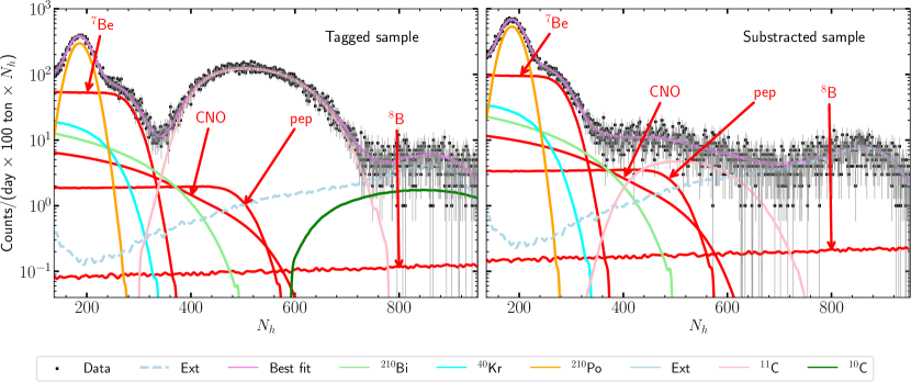
Figure 8: Spectrum for the best-fit normalizations of the different components obtained from our fit to the Borexino Phase-III data for TFC-tagged (left) and TFC-subtracted (right) events. In this figure “CNO” labels the events produced by sum of the three fluxes produced in the CNO-cycle, $\Phi_{{\mbox{}^{13}\text{N}}}+\Phi_{{\mbox{}^{15}\text{O}}}+\Phi_{{\mbox{}^{13}\text{F}}}$.

In their analysis of the different phases, the Borexino collaboration always considers a common shift in the normalization for the three fluxes of neutrinos produced in the CNO cycle with respect to their values in the SSM. On the contrary the normalization of the fluxes produced in the pp-chain are fitted independently.

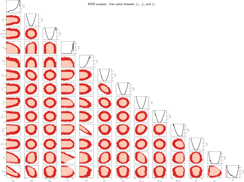
Figure 9: Same as Fig. 6 but but allowing independent variation of the normalizations of the three CNO fluxes, only subject to the consistency conditions in Eqs. (10) and (11).

In principle, once one departs from the constraints imposed by the SSM, the normalization of the three CNO fluxes could be shifted independently, subject only to the minimum set of consistency relations in Eqs. (10) and (11). In fact in our previous works Gonzalez-Garcia:2009dpj ; Bergstrom:2016cbh we could perform such general analysis. At the time there was no evidence of CNO neutrinos and therefore those analysis resulted into a more general set of upper bounds on their allowed values compared to those obtained assuming a common shift. With this as motivation, one can attempt to perform an analysis of the present BXIII spectra under the same assumption of free normalization. However, within the present modelling of the backgrounds in the Borexino analysis, optimized to provide maximum sensitivity to a positive evidence of CNO neutrinos, such generalized analysis runs into trouble as we illustrate in Fig. 9. As expected, allowing three free CNO flux normalizations results in a weaker constraints on each of the three parameters. This is particularly the case for the smaller $\mbox{}^{17}\text{F}$ flux which is allowed to take values as large as $\sim 40$ times the value predicted by the SSM without however yielding substantial $\chi^{2}$ improvements over the standard $f_{{\mbox{}^{17}\text{F}}}=1$ value. In the same way $f_{{\mbox{}^{15}\text{O}}}$ is compatible with the prediction of the SSM, $\Delta\chi^{2}(f_{{\mbox{}^{15}\text{O}}}=1)\simeq 0$, with an upper bound $f_{{\mbox{}^{15}\text{O}}}\lesssim 2$. On the contrary the fit results into a favoured range for $\mbox{}^{13}\text{N}$ which, it taken at face value, would imply an incompatibility with the SSM at large CL: $\Delta\chi^{2}(f_{{\mbox{}^{13}\text{N}}}=1)\gtrsim 6$. This large $\mbox{}^{13}\text{N}$ flux comes at a price of a very low value of the $\mbox{}^{210}\text{Bi}$ normalization, which as seen in the figure is more strongly correlated with $\mbox{}^{13}\text{N}$ than with $\mbox{}^{15}\text{O}$ and $\mbox{}^{17}\text{F}$.

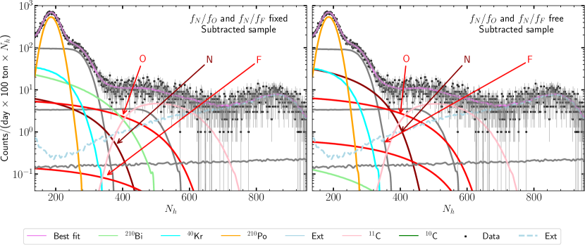
Figure 10: Spectrum of events in the TFC-subtracted sample for the best-fit normalizations of the different components obtained from two fits to the Borexino Phase-III data. In the left panel the fit is performed assuming a common normalization shift for the 3 CNO fluxes, while on the right panel the three normalizations are allowed to very free subject only the conditions Eqs. (10) and (11).

To illustrate further this point we show in Fig. 10 our best fitted spectra of the “subtracted” sample for the analysis where one common normalization for the three CNO fluxes is used (left, in what follows “CNO” fit) and the one where all the three normalizations are varied independently (right, in what follows “N” fit). Thus the spectra in the left panel of Fig. 10 are the same as the right panel of Fig. 8, except that now, for convenience, we plot separately the events from each of the CNO fluxes. This highlights clearly the different shape of the spectra of $\mbox{}^{15}\text{O}$ and $\mbox{}^{13}\text{N}$, with $\mbox{}^{15}\text{O}$ extending to larger energies. It is also evident that $\mbox{}^{13}\text{N}$ is the one mostly affected by degeneracies with the $\mbox{}^{210}\text{Bi}$ background. Comparing the two panels we see by naked eye that both spectra describe well the data: in fact, the event rates for $\mbox{}^{15}\text{O}$ are comparable in both panels. But in the right panel the normalization of the $\mbox{}^{13}\text{N}$ events is considerably enhanced while the $\mbox{}^{210}\text{Bi}$ background is suppressed: this is the option favoured by the fit.

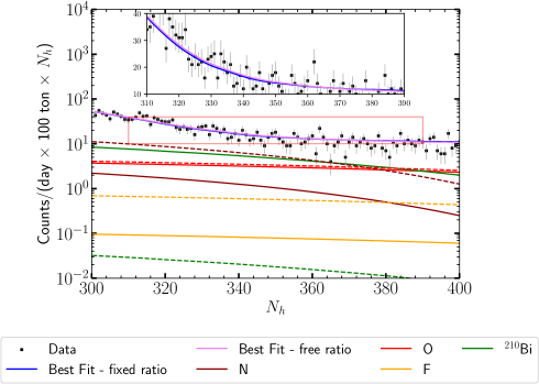
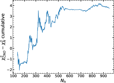
Figure 11: Left: Spectra of subtracted event rates from best fit CNO fluxes and $\mbox{}^{210}\text{Bi}$ background in the range of $300\leq N_{h}\leq 400$ for the “CNO” fit (fit with a common normalization factor for the three CNO fluxes, full lines) and the “N” fit (fit with three independent normalizations, dashed lines). We also show the best fit spectra for both fits compared to the data as labeled in the figure. Right: Difference of the value of $\chi^{2}$ in both fits as a function of the maximum $N_{h}$ bin included in the fit.

Upon closer examination we find that in the range of $N_{h}$ spanning between 300 and 400 photon hits, an increase in the value of $f_{{\mbox{}^{13}\text{N}}}$ better fits the data while driving $f_{{\mbox{}^{210}\text{Bi}}}$ towards 0. In Fig. 11 we show a blow-up of the spectra in this $N_{h}$ window. To quantify the difference in the quality of the fit for those two solutions and the relevant range of $N_{h}$ we plot in the right panel the cumulative difference of $\chi^{2}_{\text{BXIII,test}}$ for the best fits of the “CNO” and “N” fits as a function of the maximum $N_{h}$ bin included in the fit.

Clearly, this anomalously large $\mbox{}^{13}\text{N}$ solution is possible only because the sole information included in the fit for the $\mbox{}^{210}\text{Bi}$ background is the upper bound provided by the collaboration. Such upper bound is enough to ensure a lower bound on the amount of CNO neutrinos, and indeed it results in a positive evidence of CNO fluxes (in good agreement with at least some of the SSMs) when a common normalization for the three CNO fluxes is enforced, as reported by the collaboration in Refs. BOREXINO:2020aww ; BOREXINO:2022abl (and properly reproduced by us, as described in the previous section). Our results show that this is the case because the spectrum of $\mbox{}^{210}\text{Bi}$ and $\mbox{}^{15}\text{O}$ are sufficiently different. However, once the normalization of the three CNO fluxes are not linked together, the degeneracy between the spectral shape of $\mbox{}^{13}\text{N}$ and $\mbox{}^{210}\text{Bi}$ – together with the lack of a proper estimate for a lower bound on $\mbox{}^{210}\text{Bi}$ which is not quantified in Refs. BOREXINO:2020aww ; BOREXINO:2022abl  – pushes the best-fit of $\mbox{}^{13}\text{N}$ towards unnaturally large values. In other words, the background model proposed in Refs. BOREXINO:2020aww ; BOREXINO:2022abl cannot be reliably employed for fits with independent $\mbox{}^{13}\text{N}$ and $\mbox{}^{15}\text{O}$ normalizations.

We finish by noticing that this also implies that the high quality data of Borexino Phase-III, besides having been able to yield the first evidence of the presence of the CNO neutrinos, also holds the potential to discriminate between the contributions from $\mbox{}^{13}\text{N}$ and $\mbox{}^{15}\text{O}$, a potential which may be interesting to explore by the collaboration.

A.3 Analysis with Correlated Integrated Directionality Method

In a very recent work Borexino:2023puw the Borexino collaboration has presented a combined analysis of their three phases making use of the Correlated and Integrated Directionality (CID) method, which aims to enhance the precision of the determination of the flux of CNO neutrinos. In a nut-shell, the CID method exploits the sub-dominant Cherenkov light in the liquid scintillator produced by the electrons scattered in the neutrino interaction. These Cherenkov photons retain information of the original direction of the incident neutrino, hence they can be used to enhance the discrimination between the solar neutrino signal and the radioactive backgrounds.

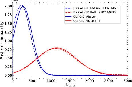
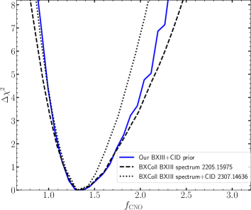
Figure 12: Left: CID posterior probabilities for the number for Phase-I and Phase-II+III of CNO-$\nu$ events after constraining pep and $\mbox{}^{8}\text{B}$ neutrino events to their SSM expectation. Right: Dependence of $\Delta\chi^{2}$ on the CNO flux normalization from our fit to the Borexino Phase-III spectra combined with the CID constraint (blue line) compared to that obtained by the Borexino collaboration (dotted black line). For comparison we also show the result without CID information (dashed black line).

Effectively, the CID analysis results into a determination of the total number of solar neutrinos detected within a restricted range of $N_{h}$ which corresponds to $0.85~{}\text{MeV}<T_{e}<1.3~{}\text{MeV}$ for Phase-I and $0.85~{}\text{MeV}<T_{e}<1.29~{}\text{MeV}$ for Phase-II+III. In this range the dominant contribution comes from CNO, pep and some $\mbox{}^{8}\text{B}$. The increased fiducial volume for this analysis brings the exposures to $740.7~{}\text{days}\times 104.3~{}\text{ton}\times 55.77\%$ for Phase-I and $2888.0~{}\text{days}\times 94.4~{}\text{ton}\times 63.97\%$ for Phase-II+III. The resulting number of solar neutrinos detected is $N^{\text{P-I}}_{\text{obs}}=643^{+235}_{-224}\text{(stat)}^{+37}_{-30}\text{(sys)}$ for Phase-I and $N^{\text{P-II+III}}_{\text{obs}}=2719^{+518}_{-494}\text{(stat)}^{+85}_{-83}\text{(sys)}$ for Phase-II+III. After subtracting the expected SSM contribution from pep and $\mbox{}^{8}\text{B}$ the Borexino collaboration obtains the posterior probability distributions for the number of CNO neutrinos shown in Fig. 9 of Ref. Borexino:2023puw (which we reproduce in the left panel in Fig. 12). Furthermore, since this new directional information is independent of the spectral information, the collaboration proceeded to combine these two priors on $N_{{\text{CNO}}}$ with the their likelihood for the Borexino Phase-III spectral analysis. This resulted in a slightly stronger dependence of the combined likelihood on the CNO-$\nu$ rate shown in their Fig. 12 (which we reproduce in the right panel in Fig. 12).

In order to account for the CID information in our analysis we try to follow as closely as possible the procedure of the collaboration. With the information provided on the covered energy range and exposures for the CID analysis, we integrate our computed spectra of solar neutrino events in each phase to derive the corresponding total number of expected events in Phase-I and Phase-II+III. We then subtract the SSM predictions for pep and $\mbox{}^{8}\text{B}$ neutrinos from the observed number of events to derive an estimate for CNO neutrinos in in Phase-I and Phase-II+III, and construct a simple Gaussian $\chi^{2}(N_{{\text{CNO}}})$ for Phase-Y (Y=I or II+III)

$$\chi^{2}_{\text{CID,P-Y}}(N_{{\text{CNO}}})=\bigg{(}\frac{N_{\text{obs}}^{\text{P-Y}}-N^{\text{P-Y}}_{\text{SSM,pep}}-N^{\text{P-Y}}_{\text{SSM,{$\mbox{}^{8}\text{B}$}}}-N_{{\text{CNO}}}}{\sigma_{\text{P-Y}}}\bigg{)}^{2}$$ (37)

where in $\sigma_{P-Y}$ we add in quadrature the symmetrized statistical and systematic uncertainties in the number of observed events.

We plot in the left panel in Fig. 12 our inferred probability distributions $P_{\text{P-Y}}(N_{{\text{CNO}}})\propto\exp[-\chi^{2}_{\text{P-Y}}/2]$ compared to those from Borexino in Fig. 9 of Ref. Borexino:2023puw . As seen in the figure our simple procedure reproduces rather well the results of the collaboration for the Phase-II+III but only reasonably for Phase-I. This may be due to differences in the reanalysis of the Phase-I data by the collaboration in the CID analysis compared to their spectral analysis of 2011. Our simulations of the Phase-I event rates are tuned to their 2011 and there is not enough information in Ref. Borexino:2023puw to deduce what may have changed. Thus we decide to introduce in our analysis the CID prior for the Phase-II+III data but not for Phase-I.

We then combine the CID from Phase-II+III and Phase-III spectral information as

$$\chi^{2}_{\text{CID+BXIII,test}}=\chi^{2}_{\text{BX-III}}+\bigg{(}\frac{f_{{\text{pep}}}-1}{\sigma_{{\text{pep}}}}\bigg{)}^{2}+\chi^{2}_{\text{CID,P-II+III}}\,.$$ (38)

A quantitative comparison with the results of the collaboration for this combined $\text{CID}+\text{Phase-III}$ spectrum analysis is shown in the right panel of Fig. 12 where we plot the dependence of our marginalized $\Delta\chi^{2}$ on the CNO flux normalization after including the CID information compared to that obtained by the collaboration in Fig. 12 of Ref. Borexino:2023puw . As seen in the figure, we reproduce well the improved sensitivity for the lower range of the CNO flux normalization but our constraints are more conservative in the higher range, though they still represent an improvement over the spectrum-only analysis.

Altogether, after all these tests and validations we define the $\chi^{2}$ for the full Borexino analysis as

$$\chi^{2}_{\text{BX}}(\vec{\omega}_{\text{osc}},\,\vec{\omega}_{\text{flux}})=\chi^{2}_{\text{BXI}}(\vec{\omega}_{\text{osc}},\,\vec{\omega}_{\text{flux}})+\chi^{2}_{\text{BXII}}(\vec{\omega}_{\text{osc}},\,\vec{\omega}_{\text{flux}})\\ +\chi^{2}_{\text{BXIII}}(\vec{\omega}_{\text{osc}},\,\vec{\omega}_{\text{flux}})+\chi^{2}_{\text{CID,P-II+III}}(\vec{\omega}_{\text{osc}},\,\vec{\omega}_{\text{flux}})\,.$$ (39)

with $\chi^{2}_{\text{BXIII}}(\vec{\omega}_{\text{osc}}\,\vec{\omega}_{\text{flux}})$ and $\chi^{2}_{\text{CID,P-II+III}}(\vec{\omega}_{\text{osc}},\vec{\omega}_{\text{flux}})$ in Eqs. (35) and (37), respectively. We finish by noticing that the inclusion of the CID information is not enough to break the large degeneracy between the $\mbox{}^{13}\text{N}$ and $\mbox{}^{210}\text{Bi}$ contributions to the spectra discussed in the previous section.

References

- (1) H.A. Bethe, Energy production in stars, Phys. Rev. 55 (1939) 434.
- (2) J.N. Bahcall, Neutrino Astrophysics, Cambridge, UK: Univ. PR. (1989) 567p (1989).
- (3) J.N. Bahcall and R.K. Ulrich, Solar Models, Neutrino Experiments and Helioseismology, Rev. Mod. Phys. 60 (1988) 297.
- (4) S. Turck-Chieze, S. Cahen, M. Casse and C. Doom, Revisiting the standard solar model, Astrophys. J. 335 (1988) 415.
- (5) J.N. Bahcall and M.H. Pinsonneault, Standard solar models, with and without helium diffusion and the solar neutrino problem, Rev. Mod. Phys. 64 (1992) 885.
- (6) J.N. Bahcall and M.H. Pinsonneault, Solar models with helium and heavy element diffusion, Rev. Mod. Phys. 67 (1995) 781 [hep-ph/9505425].
- (7) J.N. Bahcall, M.H. Pinsonneault and S. Basu, Solar models: Current epoch and time dependences, neutrinos, and helioseismological properties, Astrophys. J. 555 (2001) 990 [astro-ph/0010346].
- (8) J.N. Bahcall, A.M. Serenelli and S. Basu, New solar opacities, abundances, helioseismology, and neutrino fluxes, Astrophys. J. 621 (2005) L85 [astro-ph/0412440].
- (9) C. Pena-Garay and A. Serenelli, Solar neutrinos and the solar composition problem, 0811.2424.
- (10) A.M. Serenelli, W.C. Haxton and C. Pena-Garay, Solar models with accretion. I. Application to the solar abundance problem, Astrophys. J. 743 (2011) 24 [1104.1639].
- (11) N. Vinyoles, A.M. Serenelli, F.L. Villante, S. Basu, J. Bergström, M.C. Gonzalez-Garcia et al., A new Generation of Standard Solar Models, Astrophys. J. 835 (2017) 202 [1611.09867].
- (12) J.N. Bahcall, Solar neutrinos. I: Theoretical, Phys. Rev. Lett. 12 (1964) 300.
- (13) J.N. Bahcall, N.A. Bahcall and G. Shaviv, Present status of the theoretical predictions for the Cl-36 solar neutrino experiment, Phys. Rev. Lett. 20 (1968) 1209.
- (14) J.N. Bahcall and R. Davis, Solar Neutrinos - a Scientific Puzzle, Science 191 (1976) 264.
- (15) B. Pontecorvo, Neutrino experiments and the problem of conservation of leptonic charge, Sov. Phys. JETP 26 (1968) 984.
- (16) V. Gribov and B. Pontecorvo, Neutrino astronomy and lepton charge, Phys. Lett. B28 (1969) 493.
- (17) L. Wolfenstein, Neutrino Oscillations in Matter, Phys. Rev. D17 (1978) 2369.
- (18) S.P. Mikheev and A.Y. Smirnov, Resonance Amplification of Oscillations in Matter and Spectroscopy of Solar Neutrinos, Sov. J. Nucl. Phys. 42 (1985) 913. [Yad. Fiz.42,1441(1985)].
- (19) N. Grevesse and A.J. Sauval, Standard Solar Composition, Space Sci. Rev. 85 (1998) 161.
- (20) M. Asplund, N. Grevesse, A.J. Sauval and P. Scott, The Chemical Composition of the Sun, ARA&A 47 (2009) 481 [0909.0948].
- (21) J.N. Bahcall, S. Basu, M. Pinsonneault and A.M. Serenelli, Helioseismological implications of recent solar abundance determinations, Astrophys. J. 618 (2005) 1049 [astro-ph/0407060].
- (22) M. Castro, S. Vauclair and O. Richard, Low abundances of heavy elements in the solar outer layers: comparisons of solar models with helioseismic inversions, Astron. & Astrophys. 463 (2007) 755 [astro-ph/0611619].
- (23) J.A. Guzik and K. Mussack, Exploring Mass Loss, Low-Z Accretion, and Convective Overshoot in Solar Models to Mitigate the Solar Abundance Problem, Astrophys. J. 713 (2010) 1108 [1001.0648].
- (24) A. Serenelli, S. Basu, J.W. Ferguson and M. Asplund, New Solar Composition: The Problem With Solar Models Revisited, Astrophys. J. 705 (2009) L123 [0909.2668].
- (25) M.C. Gonzalez-Garcia, M. Maltoni and J. Salvado, Direct determination of the solar neutrino fluxes from solar neutrino data, JHEP 05 (2010) 072 [0910.4584].
- (26) J. Bergstrom, M.C. Gonzalez-Garcia, M. Maltoni, C. Pena-Garay, A.M. Serenelli and N. Song, Updated determination of the solar neutrino fluxes from solar neutrino data, JHEP 03 (2016) 132 [1601.00972].
- (27) Borexino collaboration, First Simultaneous Precision Spectroscopy of , 7Be, and Solar Neutrinos with Borexino Phase-II, Phys. Rev. D 100 (2019) 082004 [1707.09279].
- (28) Borexino collaboration, Improved Measurement of Solar Neutrinos from the Carbon-Nitrogen-Oxygen Cycle by Borexino and Its Implications for the Standard Solar Model, Phys. Rev. Lett. 129 (2022) 252701 [2205.15975].
- (29) Borexino collaboration, Final results of Borexino on CNO solar neutrinos, 2307.14636.
- (30) M. Asplund, A.M. Amarsi and N. Grevesse, The chemical make-up of the Sun: A 2020 vision, arXiv e-prints (2021) arXiv:2105.01661 [2105.01661].
- (31) E. Magg et al., Observational constraints on the origin of the elements - IV. Standard composition of the Sun, Astron. Astrophys. 661 (2023) A140 [2203.02255].
- (32) GALLEX collaboration, Final results of the Cr-51 neutrino source experiments in GALLEX, Phys. Lett. B 420 (1998) 114.
- (33) F. Kaether, W. Hampel, G. Heusser, J. Kiko and T. Kirsten, Reanalysis of the GALLEX solar neutrino flux and source experiments, Phys. Lett. B685 (2010) 47 [1001.2731].
- (34) SAGE collaboration, Measurement of the response of the Russian-American gallium experiment to neutrinos from a Cr-51 source, Phys. Rev. C 59 (1999) 2246 [hep-ph/9803418].
- (35) J.N. Abdurashitov et al., Measurement of the response of a Ga solar neutrino experiment to neutrinos from an Ar-37 source, Phys. Rev. C 73 (2006) 045805 [nucl-ex/0512041].
- (36) V.V. Barinov et al., Results from the Baksan Experiment on Sterile Transitions (BEST), Phys. Rev. Lett. 128 (2022) 232501 [2109.11482].
- (37) V.V. Barinov et al., Search for electron-neutrino transitions to sterile states in the BEST experiment, Phys. Rev. C 105 (2022) 065502 [2201.07364].
- (38) V. Brdar, J. Gehrlein and J. Kopp, Towards resolving the gallium anomaly, JHEP 05 (2023) 143 [2303.05528].
- (39) J.M. Berryman, P. Coloma, P. Huber, T. Schwetz and A. Zhou, Statistical significance of the sterile-neutrino hypothesis in the context of reactor and gallium data, JHEP 02 (2022) 055 [2111.12530].
- (40) C. Giunti, Y.F. Li, C.A. Ternes and Z. Xin, Inspection of the detection cross section dependence of the Gallium Anomaly, Phys. Lett. B 842 (2023) 137983 [2212.09722].
- (41) S.R. Elliott, V.N. Gavrin, W.C. Haxton, T.V. Ibragimova and E.J. Rule, Gallium neutrino absorption cross section and its uncertainty, Phys. Rev. C 108 (2023) 035502 [2303.13623].
- (42) B.T. Cleveland et al., Measurement of the solar electron neutrino flux with the Homestake chlorine detector, Astrophys. J. 496 (1998) 505.
- (43) SAGE collaboration, Measurement of the solar neutrino capture rate with gallium metal. III: Results for the 2002–2007 data-taking period, Phys. Rev. C80 (2009) 015807 [0901.2200].
- (44) Super-Kamiokande collaboration, Solar neutrino measurements in Super-Kamiokande-I, Phys. Rev. D73 (2006) 112001 [hep-ex/0508053].
- (45) Super-Kamiokande collaboration, Solar neutrino measurements in Super-Kamiokande-II, Phys. Rev. D78 (2008) 032002 [0803.4312].
- (46) Super-Kamiokande collaboration, Solar neutrino results in Super-Kamiokande-III, Phys. Rev. D83 (2011) 052010 [1010.0118].
- (47) Y. Nakajima, “Recent results and future prospects from Super-Kamiokande.” Talk given at the XXIX International Conference on Neutrino Physics and Astrophysics, Chicago, USA, June 22–July 2, 2020 (online conference).
- (48) SNO collaboration, Combined Analysis of all Three Phases of Solar Neutrino Data from the Sudbury Neutrino Observatory, 1109.0763.
- (49) Borexino collaboration, Precision measurement of the 7Be solar neutrino interaction rate in Borexino, Phys. Rev. Lett. 107 (2011) 141302 [1104.1816].
- (50) KamLAND collaboration, Reactor On-Off Antineutrino Measurement with KamLAND, Phys. Rev. D88 (2013) 033001 [1303.4667].
- (51) Herrera, Y. and Serenelli, A., “ChETEC-INFRA WP8: Astronuclear Library: Standard Solar Models B23.” https://doi.org/10.5281/zenodo.10174172.
- (52) I. Esteban, M.C. Gonzalez-Garcia, M. Maltoni, T. Schwetz and A. Zhou, “NuFIT 5.2 (2022).” http://www.nu-fit.org.
- (53) F. Feroz, M.P. Hobson, E. Cameron and A.N. Pettitt, Importance Nested Sampling and the MultiNest Algorithm, Open J. Astrophys. 2 (2019) 10 [1306.2144].
- (54) F. Feroz, M.P. Hobson and M. Bridges, MultiNest: an efficient and robust Bayesian inference tool for cosmology and particle physics, Mon. Not. Roy. Astron. Soc. 398 (2009) 1601 [0809.3437].
- (55) GAMBIT collaboration, Comparison of statistical sampling methods with ScannerBit, the GAMBIT scanning module, Eur. Phys. J. C 77 (2017) 761 [1705.07959].
- (56) M. Spiro and D. Vignaud, Solar Model Independent Neutrino Oscillation Signals in the Forthcoming Solar Neutrino Experiments?, Phys. Lett. B242 (1990) 279. [,609(1990)].
- (57) J.N. Bahcall, The Luminosity constraint on solar neutrino fluxes, Phys. Rev. C65 (2002) 025801 [hep-ph/0108148].
- (58) D. Vescovi, C. Mascaretti, F. Vissani, L. Piersanti and O. Straniero, The luminosity constraint in the era of precision solar physics, Journal of Physics G Nuclear Physics 48 (2021) 015201 [2009.05676].
- (59) L.J. Frohlich C., The Sun’s total irradiance: cycles,trends and related climate change uncertainties since 1978, Geophys. Res. Lett. 25 (1998) 4377.
- (60) L.J. Kopp G., A New, Lower Value of Total Solar Irradiance: Evidence and Climate Significance., Geophys. Res. Lett. 38 (2011) L01706.
- (61) N. Scafetta and R.C. Willson, ACRIM total solar irradiance satellite composite validation versus TSI proxy models, Astrophysics and Space Science 350 (2014) 421.
- (62) Particle Data Group collaboration, Review of Particle Physics, PTEP 2022 (2022) 083C01.
- (63) J.N. Bahcall and P.I. Krastev, How well do we (and will we) know solar neutrino fluxes and oscillation parameters?, Phys. Rev. D53 (1996) 4211 [hep-ph/9512378].
- (64) Borexino collaboration, Experimental evidence of neutrinos produced in the CNO fusion cycle in the Sun, Nature 587 (2020) 577 [2006.15115].
- (65) M. Laveder, Unbound neutrino roadmaps, Nucl. Phys. B Proc. Suppl. 168 (2007) 344.
- (66) M.A. Acero, C. Giunti and M. Laveder, Limits on nu(e) and anti-nu(e) disappearance from Gallium and reactor experiments, Phys. Rev. D 78 (2008) 073009 [0711.4222].
- (67) C. Giunti and M. Laveder, Statistical Significance of the Gallium Anomaly, Phys. Rev. C 83 (2011) 065504 [1006.3244].
- (68) M. Maltoni and T. Schwetz, Testing the statistical compatibility of independent data sets, Phys. Rev. D 68 (2003) 033020 [hep-ph/0304176].
- (69) Borexino collaboration, Measurement of the solar 8B neutrino rate with a liquid scintillator target and 3 MeV energy threshold in the Borexino detector, Phys. Rev. D82 (2010) 033006 [0808.2868].
- (70) P. Coloma, M. Gonzalez-Garcia, M. Maltoni, J.a.P. Pinheiro and S. Urrea, Constraining new physics with Borexino Phase-II spectral data, JHEP 07 (2022) 138 [2204.03011]. [Erratum: JHEP 11, 138 (2022)].
- (71) Borexino collaboration, ‘‘Improved measurement of solar neutrinos from the carbon-nitrogen-oxygen cycle by borexino and its implications for the standard solar model.’’ https://borex.lngs.infn.it/category/opendata/.
- (72) N. Rossi. Private communication.
- (73) M. Maltoni, From ray to spray: augmenting amplitudes and taming fast oscillations in fully numerical neutrino codes, JHEP 11 (2023) 033 [2308.00037].