Properties of the Magellanic Corona Model for the formation of the Magellanic Stream

Abstract

We characterize the Magellanic Corona model of the formation of the Magellanic Stream, which we introduced in Lucchini et al. (2020, 2021). Using high-resolution hydrodynamic simulations, we constrain the properties of the primordial Magellanic Clouds, including the Magellanic Corona – the gaseous halo around the Large Magellanic Cloud (LMC). With an LMC mass of $1.75\times 10^{11}$ $\mathrm{M}_{\odot}$, a Magellanic Corona of $>5\times 10^{9}$ $\mathrm{M}_{\odot}$ at $3\times 10^{5}$ K, a total Small Magellanic Cloud mass $<10^{10}$ $\mathrm{M}_{\odot}$, and a Milky Way corona of $2\times 10^{10}$ $\mathrm{M}_{\odot}$, we can reproduce the observed total mass of the neutral and ionized components of the Trailing Stream, ionization fractions along the Stream, morphology of the neutral gas, and on-sky extent of the ionized gas. The inclusion of advanced physical routines in the simulations allow the first direct comparison of a hydrodynamical model with UV absorption-line spectroscopic data. Our model reproduces O I, O VI, and C IV observations from HST/COS and FUSE. The stripped material is also nearby ($<50$ kpc from the Sun), as found in our prior models including a Magellanic Corona.

[1em]0em0em

1 Introduction

The Magellanic Stream is the largest coherent extragalactic gaseous structure in our sky (Mathewson et al., 1974). It has the potential to dramatically impact the future of the Milky Way (MW) by depositing billions of solar masses of gas into our circumgalactic medium (CGM) and possibly onto our disk (Fox et al., 2014; D’Onghia & Fox, 2016). The Magellanic Stream also provides direct evidence of galaxy interactions and evolution through mergers. By studying this serendipitous nearby system, we will learn about the future of our own Galaxy, the history of the Local Group, and the gas and metal transport processes that can sustain the growth of galaxies like the MW.

The Magellanic Stream is an extended network of interwoven clumpy filaments of gas that originate from within the Large and Small Magellanic Clouds (LMC, SMC), two dwarf galaxy satellites of the MW. Combined with the Leading Arm, high velocity clumps of gas ahead of the Magellanic Clouds in their orbits, the Magellanic System covers over 200^∘ on the sky. From 21-cm H I observations, we have an excellent view of its small-scale, turbulent morphology as well as its velocity structure (e.g. Cohen, 1982; Morras, 1983; Putman et al., 2003; Brüns et al., 2005; Nidever et al., 2008, 2010; Westmeier, 2018). Moreover, absorption line spectroscopy studies have characterized the chemical composition and ionization state of the Stream along dozens of sightlines (Lu et al., 1994; Gibson et al., 2000; Sembach et al., 2003; Fox et al., 2010, 2013, 2014; Richter et al., 2013). Fox et al. (2014) has shown that the Stream is mostly ionized. They find an average ionization fraction of $\approx$73% with a total ionized gas mass of $\sim 1.5\times 10^{9}$ $\mathrm{M}_{\odot}$ (compared with $4.9\times 10^{8}$ $\mathrm{M}_{\odot}$ of neutral gas; Brüns et al. 2005).

Models of the formation of the Stream originally explained the stripped material as gas that was tidally pulled from the LMC through repeated interactions with the MW (Fujimoto & Sofue, 1976; Davies & Wright, 1977; Lin & Lynden-Bell, 1977, 1982; Gardiner & Noguchi, 1996; Connors et al., 2006; Diaz & Bekki, 2011). This would result not only in stripped gas, but also in a tidally truncated dark matter halo. Thus, masses determined by rotation curve fitting ($1.7\pm 0.7\times 10^{10}$ $\mathrm{M}_{\odot}$ within 8.7 kpc, van der Marel & Kallivayalil, 2014) would be sufficient for modeling the evolution of the Clouds and the formation of the Stream. However, updated proper-motion measurements of the LMC and SMC have shown that the Clouds are most likely on their first infall towards the Milky Way (Kallivayalil et al., 2006; Besla et al., 2007; Kallivayalil et al., 2013). A recent study has found a second passage orbit consistent with the observations, however further studies of the hydrodynamics are required to see if the Stream can be reproduced (Vasiliev, 2024). A first-infall scenario would require a higher LMC mass as it would not yet be tidally truncated. Many different indirect methods of estimating the LMC’s total pre-infall mass have converged on a value of $1-2\times 10^{11}$ $\mathrm{M}_{\odot}$: $1.98\times 10^{11}$ $\mathrm{M}_{\odot}$ from abundance matching (Read & Erkal, 2019), $>$10¹¹ $\mathrm{M}_{\odot}$ from the MW’s reflex motion (Petersen & Peñarrubia, 2021), $>$1.24$\times 10^{11}$ $\mathrm{M}_{\odot}$ from the LMC’s satellite population (Erkal & Belokurov, 2020), $2.5^{+0.09}_{-0.08}\times 10^{11}$ $\mathrm{M}_{\odot}$ from the Hubble flow timing argument (Peñarrubia et al., 2016), and $1-2\times 10^{11}$ $\mathrm{M}_{\odot}$ from the MW’s stellar streams (Erkal et al., 2019; Shipp et al., 2021). See Figure 1 for a summary. Shown in this figure is also the error-weighted mean of the values calculated in Vasiliev et al. (2021), Shipp et al. (2021), Erkal et al. (2019), Read & Erkal (2019), and Peñarrubia et al. (2016): $1.60\pm 0.21\times 10^{11}$ $\mathrm{M}_{\odot}$ ($\sim 10-20$% of the MW’s total mass).

While modern tidal models of the formation of the Stream have used large masses for the LMC, they are unable to explain the immense ionized mass (Besla et al., 2010, 2012; Pardy et al., 2018). On the other hand, ram pressure models (Meurer et al., 1985; Moore & Davis, 1994; Sofue, 1994) are able to explain the ionized material via dissolution of the neutral gas through instabilities, but they require low masses for the LMC ($<2\times 10^{10}$ $\mathrm{M}_{\odot}$; Hammer et al., 2015; Wang et al., 2019).

To resolve both of these discrepancies simultaneously, we introduced the Magellanic Corona model (Lucchini et al. 2020, 2021, hereafter L20, L21). Based on theoretical calculations and cosmological simulations, galaxies with masses $\sim 10^{11}$ $\mathrm{M}_{\odot}$ should host gaseous halos at their virial temperature of $\sim 3\times 10^{5}$ K (Jahn et al., 2021). Upon inclusion of a warm CGM around the LMC, dubbed the Magellanic Corona, we are able to explain the ionized material in the Stream while accounting for a massive LMC. In L21, we showed that this Magellanic Corona also exerts hydrodynamical drag on the SMC as it orbits around the LMC. With a new orbital history consistent with the present-day positions and velocities of the Clouds, the Trailing Stream ends up five times closer to us than previous models predicted. The Magellanic Corona model is described in more detail in Section 1.1.

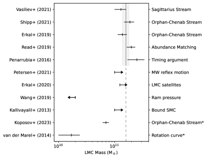
Figure 1: Observational LMC total mass estimates. Literature estimates for the total mass of the Large Magellanic Cloud. van der Marel & Kallivayalil (2014) and Koposov et al. (2023) (denoted with asterisks) provide constraints on the mass within 8.7 and 32.4 kpc, respectively, whereas all other estimates plotted are for the total virial LMC mass. Kallivayalil et al. (2013), Erkal & Belokurov (2020), and Petersen & Peñarrubia (2021) provide lower limits, and Wang et al. (2019) provides an upper limit. The remaining references (Peñarrubia et al., 2016; Read & Erkal, 2019; Erkal et al., 2019; Shipp et al., 2021; Vasiliev et al., 2021) give estimates of the total LMC mass with uncertainties. The error weighted average of these five values is $1.60\pm 0.21\times 10^{11}$ shown as the vertical line (extended to the bottom of the plot as a dashed line for comparison). The one-sigma errors are shown as a shaded region. The method for determining the LMC mass estimate from each paper is listed on the right edge of the plot.

In a subsequent study, the Magellanic Corona was directly observed using absorption line spectroscopy data from the Cosmic Origins Spectrograph on the Hubble Space Telescope (Krishnarao et al., 2022). From 28 sightlines extending to 35 kpc away from the LMC, we detected a radially declining profile in high ions (C IV, Si IV, O VI) with a total mass of $1.4\pm 0.6\times 10^{9}$ $\mathrm{M}_{\odot}$ including a warm phase with temperature of $3\times 10^{5}$ K. These results are consistent with the picture of a first-infall LMC with a Magellanic Corona. While these values give us an excellent picture of the LMC’s CGM at the present-day, modeling the evolution of the Magellanic System will help us constrain the properties of the primordial LMC and its Magellanic Corona to understand dwarf galaxy evolution in general.

1.1 History of the Magellanic Corona Model

In L20, we presented a model of the evolution of the Stream including the Magellanic Corona, showing that we can reproduce the total mass budget of the Stream including its ionized component. This model also forms and extended Trailing Stream and Leading Arm through tidal interactions between the Clouds. In this work, we used previously published orbital histories for the Clouds (Besla et al., 2012; Pardy et al., 2018); however, the Magellanic Corona exerts hydrodynamic drag forces on the SMC as it orbits around the LMC, so the kinematics and positions of the Magellanic Clouds were not in agreement with observations in this proof-of-concept study.

In order to match the present-day positions and velocities of the LMC and the SMC, we then explored the orbital histories of the Clouds (L21). In the updated orbit published in this work (still including the Magellanic Corona), the 3D velocities of the Clouds agree with the observed values within 3$\sigma$. Additionally, due to the hydrodynamic interactions of the tidally stripped (neutral) material with the Magellanic and Galactic Coronae, we reproduce the turbulent, filamentary structures within the H I Trailing Stream. This orbital history is shorter than previous models, and so there is no time for a Leading Arm to form, and the large-scale morphology of the Trailing Stream is different than the observations. However, the stripped gas in this model ends up very near the Sun ($<50$ kpc) which is in contrast to previous predictions ($>100-200$ kpc; Besla et al. 2012). A nearby Stream is able to explain a number of other inconsistencies between the observations and previous models: pressure equilibrium (Wolfire et al., 1995), the numerous head-tail clouds (Putman et al., 2003; For et al., 2014), and the H$\alpha$ emission (Bland-Hawthorn et al., 2013, 2019; Barger et al., 2017). Both of these previous publications have included simplistic models for star formation and temperature evolution, which is improved upon in this work.

In this paper, we expand upon the Magellanic Corona model by presenting new, high-resolution simulations with detailed physical models including the self-consistent tracking of star formation, feedback, ionization, and metallicity to directly compare with absorption line spectroscopy observations. Furthermore, we explore the parameter space of temperatures and densities for the Magellanic and Galactic Coronae that provide the best match to the observed properties of the Magellanic Clouds as well as the morphology of the neutral H I Stream. In Section 2, we outline the methodology of our simulations and analysis. Section 3 presents our simulated present-day Stream including the updated physical models and new galaxy initial conditions. In Section 4, we discuss our parameter space exploration of the properties of the Magellanic Corona. Section 5 contains the discussion of our results and the implications for the properties of the MW’s CGM. We conclude in Section 6.

Table 1: Initial Properties of the Galaxies.

	LMC ($t=0$ Gyr)	LMC ($t=3.5$ Gyr)	SMC ($t=0$ Gyr)
DM Mass ($\mathrm{M}_{\odot}$)	$1.75\times 10^{11}$	$1.75\times 10^{11}$	$5\times 10^{9}$
Stellar Disk Mass ($\mathrm{M}_{\odot}$)	$2.5\times 10^{9}$	$2.7\times 10^{9}$	$2.5\times 10^{8}$
Stellar Scale Length (kpc)	4.5	4.2	1.7
Gaseous Disk Mass ($\mathrm{M}_{\odot}$)	0	$9.1\times 10^{8}$	$1.5\times 10^{9}$
Gaseous Scale Length (kpc)	–	5.2	6.9
CGM Mass ($\mathrm{M}_{\odot}$)	$5\times 10^{9}$	$3.7\times 10^{9}$	–
CGM Temperature (K)	$3\times 10^{5}$	$3.4\times 10^{5}$	–
N Particles	$5.5\times 10^{5}$	$5.5\times 10^{5}$	$8.5\times 10^{4}$
Initial Position (kpc)	–	($33.03$, $584.97$, $300.80$)	($-21.40$, $610.74$, $357.15$)
Initial Velocity (km s-1)	–	($2.24$, $-63.93$, $-65.77$)	($6.05$, $10.48$, $-109.69$)

2 Methods

We use gizmo, a massively parallel, multiphysics code for our simulations (Hopkins, 2015; Springel, 2005). We utilize its Lagrangian “meshless finite-mass” hydrodynamics scheme which allows for the ability to track individual fluid elements while conserving angular momentum and capturing shocks (Hopkins, 2015). Star formation is included (Springel & Hernquist, 2003) with a physical density threshold of 100 cm^-3, a virial requirement that the gas is locally self-gravitating (Hopkins et al., 2013, 2018), and a requirement that the gas is converging ($\nabla\cdot v<0$). Mechanical stellar feedback is also included in which we assume a constant supernova rate of $3\times 10^{-4}$ SNe Myr^-1 $\mathrm{M}_{\odot}^{-1}$ for all stars less than 30 Myr old. Each supernova injects 14.8 $\mathrm{M}_{\odot}$ with $10^{51}$ ergs of energy and metals following the AGORA model (Kim et al., 2016). Cooling is included down to $\sim 10$ K following Hopkins et al. (2018) with metal-dependent tables (Wiersma et al., 2009). We don’t include radiative transfer or UV background radiation, however outside the MW at low redshift, we don’t expect these mechanisms to play a significant role.

These simulations improve upon those of L20 and L21 by including accurate star formation and feedback with metallicity and advanced cooling routines. gizmo calculates self-consistent ionization states for each particle based on collisional heating/ionization, recombination, free-free emission, high and low temperature metal-line cooling, and compton heating/cooling (see Appendix B in Hopkins et al., 2018) We therefore are able to track the neutral and ionized material separately throughout the simulation.

2.1 Initial Conditions

Table 1 shows the properties of the Magellanic Clouds in our simulation and we used the dice code to generate our initial conditions (Perret et al., 2014). We used an LMC dark matter (DM) mass of $1.75\times 10^{11}$ $\mathrm{M}_{\odot}$ consistent with previous studies (Besla et al. 2012; Pardy et al. 2018; ; ) and in agreement with indirect estimations (see Figure 1). We constrained the initial gaseous and stellar disk masses for the Magellanic Clouds by requiring their present-day values to be consistent with observations. This was straight forward for the stellar masses as the stars formed during the simulations comprise only a small fraction of the total. However the gas masses can vary greatly from their initial values due to the tidal interactions and accretion from the Magellanic Corona. We found that the LMC’s disk gas mass agreed best with present-day values when allowing the gaseous disk to form naturally out of the Magellanic Corona. Therefore, we initialize our fiducial LMC ($t=0$ Gyr in Table 1) with a $2.5\times 10^{9}$ $\mathrm{M}_{\odot}$ stellar disk and a Magellanic Corona with total mass (within 200 kpc) of $5\times 10^{9}$ $\mathrm{M}_{\odot}$ following an isothermal profile at a temperature of $3\times 10^{5}$ K and a metallicity of 0.1 solar. After 3.5 Gyr in isolation, there remains $3.7\times 10^{9}$ $\mathrm{M}_{\odot}$ of ionized material bound to the LMC (with $2\times 10^{9}$ $\mathrm{M}_{\odot}$ within 120 kpc) with a median temperature of $3.4\times 10^{5}$ K. $9.1\times 10^{8}$ $\mathrm{M}_{\odot}$ has cooled to form the LMC’s gaseous disk. This is the LMC that we start with for the full simulations with the LMC, SMC, and MW (listed as “LMC ($t=3.5$ Gyr)” in Table 1). The initial and final radial density and temperature profiles are shown in Figure 2 in blue. A parameter space exploration of optimal masses and temperatures for the Magellanic Corona is discussed in Section 4.

The only constraint on the SMC’s total mass comes from its rotation curve which requires $2.4\pm 0.36\times 10^{9}$ $\mathrm{M}_{\odot}$ within 4 kpc ($1.25\pm 0.25\times 10^{9}$ $\mathrm{M}_{\odot}$ in DM; Di Teodoro et al. 2019). While previous studies found that $\sim 10\%$ of the LMC’s total mass ($\sim 2\times 10^{10}$ $\mathrm{M}_{\odot}$) produced the best results (Pardy et al., 2018), this was prior to the inclusion of the Magellanic and Galactic Coronae. Therefore, in this study we have explored the effect of the SMC total mass on the formation of the Stream and found that a lower SMC mass provides better results. In our fiducial model, we used a DM mass of $5\times 10^{9}$ $\mathrm{M}_{\odot}$, a stellar mass of $2.5\times 10^{8}$ $\mathrm{M}_{\odot}$, and a gaseous disk mass of $1.5\times 10^{9}$ $\mathrm{M}_{\odot}$ (listed in Table 1).

For the MW, we implemented a live DM halo with a total mass of $1.1\times 10^{12}$ $\mathrm{M}_{\odot}$ combined with a hot gaseous CGM following a $\beta$-profile as in Salem et al. (2015):

$$\rho\propto\left[1+\left(\frac{r}{r_{c}}\right)^{2}\right]^{-3\beta/2}$$ (1)

with $r_{c}=0.35$ and $\beta=0.559$. As with the Magellanic Corona, we explored a variety of models for the Galactic corona as well, which will be discussed in Section 5.1. Our fiducial MW CGM has a total mass of $2\times 10^{10}$ $\mathrm{M}_{\odot}$ at $10^{6}$ K and is nonrotating. After evolution in isolation for 2 Gyr, $1.9\times 10^{10}$ $\mathrm{M}_{\odot}$ remains bound with a mean temperature of $1.4\times 10^{6}$ K. Figure 2 shows the initial and final (after 2 Gyr in isolation) density and temperature profiles in orange.

We use a mass resolution of $\sim 3\times 10^{4}$ $\mathrm{M}_{\odot}$/particle for the gas elements, $\sim 2\times 10^{4}$ $\mathrm{M}_{\odot}$/particle for the stars, $\sim 10^{6}$ $\mathrm{M}_{\odot}$/particle for the DM. This results in a total particle number of $1.5\times 10^{6}$. Adaptive softening was used for the gas particles (such that the hydrodynamic smoothing lengths are the same as the gravitational softening length), and softening lengths of 150 pc and 550 pc were used for the stellar and dark matter particles, respectively.

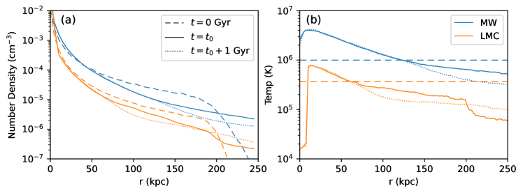
Figure 2: Initial properties of the Magellanic and Galactic Coronae. The Magellanic Corona is shown in orange and the MW corona is shown in blue. The dashed lines shows the profiles at $t=0$ Gyr, and the solid lines show the profiles at the end of isolated evolution ($t_{0}=2$ Gyr for the MW, and $t_{0}=3.5$ Gyr for the LMC). The dotted lines show the profiles after an additional 1 Gyr of evolution. Panel a shows the number density and panel b shows the median temperature as functions of radius.

2.2 Orbits of the Clouds

Following L21, we have determined viable orbital histories for the Clouds with analytic integration. Using the galactic dynamics code gala (Price-Whelan, 2017; Price-Whelan et al., 2022), we varied the present-day positions and velocities of the Clouds within their errors (Di Teodoro et al., 2019; Graczyk et al., 2020; De Leo et al., 2020; Wan et al., 2020) and integrated them backwards in time considering the effects of the MW, dynamical friction, and an empirical hydrodynamical friction term. With slight alterations to the initial positions and velocities, we obtained the initial conditions for our full hydrodynamic simulations using gizmo. Many of the orbits determined by the gala integrations were not viable once the hydrodynamics were included. This was for a variety of reasons including, for example, extremely low impact parameter collisions, tidal forces not stripping material in the correct direction, and mass loss and nonaxisymmetric effects of the live dark matter haloes. Upon visual inspection, we determined which gala orbits should be interated on and we improved the visual appearance of the Trailing Stream, and the positions and velocities of the Clouds at the present day. Our fiducial orbit used in the simulations presented here consists of two interactions over 4.2 Gyr, very similar to the orbits presented in L21. The initial properties of the Clouds as well as their positions and velocities (relative to the MW located at the origin) are listed in Table 1.

3 The Neutral Stream

As shown in L21, the inclusion of the Magellanic Corona leads to a family of orbital histories in which the Stream ends up within 50 kpc from the Sun. The previous first-infall history predicted the Trailing Stream at $>100$ kpc (Besla et al., 2012), however the hydrodynamical friction on the SMC as it orbits the LMC in the Magellanic Corona model requires fewer interactions and a shorter interaction history. As the stripped material moves through the Magellanic Corona and approaches the MW’s corona, it is encountering hot gas. In order for the neutral Stream to survive to the present day, the gas stripped out of the SMC must be dense enough to remain neutral (e.g. Bustard & Gronke 2022).

As we will see in Sections 4 and 5.1, the properties of the Magellanic and Galactic Coronae are largely determined by their stability. We therefore varied the properties of the Clouds themselves to ensure that the neutral Stream survives to the present day. Reducing the total DM mass of the SMC reduces its density, therefore making the potential well of the galaxy shallower, allowing for more material to be tidally stripped during its interactions with the LMC. For SMC DM masses below $10^{10}$ $\mathrm{M}_{\odot}$, we find that there is enough gas stripped such that the neutral Stream survives its passage through the surrounding hot gas.

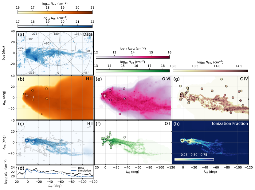
Figure 3: Properties of the Stream in the Magellanic Corona model. The properties of our simulated Stream compared with observations. Panel a shows the observed neutral 21 cm H I column density in blue from Nidever et al. (2010) in Magellanic coordinates with Galactic coordinates overlaid. Panel c shows the H I content in our simulated Stream with the observations from Panel a overlaid as contours. Panel d compares the integrated column density vs Magellanic Longitude of the observations (black) with our model (blue). Panels b, e, f, and g show column densities for H II, O VI, O I, and C IV (respectively) of the simulated Stream in the background with observational data from absorption spectra shown as points (colored based on observed column density using the same colorbar). The O VI and O I data are from Krishnarao et al. (2022), while the C IV data are from Fox et al. (2014), and the H II data are inferred from C IV via ionization modeling (Krishnarao et al., 2022). Finally, Panel h shows the ionization fraction throughout the Stream in our simulation ($x_{\mathrm{HII}}=\,$N(H II)/(N(H I) + N(H II))). The plus marks in the six central panels denote the locations of the LMC and SMC at the present day.

Figure 3 shows the results of our fiducial simulation in Magellanic Coordinates. The observational H I 21cm emission data from Nidever et al. (2010) is shown in Panel a. Panels b and c show, respectively, the H II and H I emission in our simulation with H II column densities calculated via CLOUDY ionization modeling overlaid as colored data points (data from Krishnarao et al. 2022). The H II distribution shows that the ionized material forms a cocoon around the neutral material covering a significant fraction of the sky. The neutral material consists of two filaments with turbulent, non-uniform structure, agreeing well with the morphology of the observations. As with the model presented in L21, no Leading Arm is formed due to the short interaction history and specific orbital orientation. Panel d shows the column density integrated along Magellanic Latitude as a function of Magellanic Longitude. The observations are shown in black and the simulation in blue. While we slightly underpredict the total column, the decreasing density as a function of longitude agrees well.

Panels e, f, and g show corresponding representations for the metal content in the Stream with O VI, O I, and C IV respectively. These panels also include observational column densities calculated from absorption line spectra (oxygen data from Krishnarao et al. 2022; C IV data from Fox et al. 2014). Here we see that the O VI traces the Magellanic Corona well with a large covering fraction, and the O I contains many of the same features as we see in the H I. The C IV distribution is quite variable which is represented in the observations as well. The overall sky coverage of the observed C IV is not reproduced very well in our model due to the fact that C IV is comprised of two phases: a photoionized phase, and a collisionally ionized phase. The photoionized phase exists at the warm boundary between the cold, neutral material, and the hot, ionized gas. For this reason it traces the neutral gas as we see in the model. However, the collisionally phase of C IV is in the diffuse warm gas surrounding the Clouds. Due to the interaction between the Magellanic Corona and the MW’s CGM, the Corona is heated above $5\times 10^{5}$ K to temperatures at which C IV is suppressed, in contrast with the observations. With higher resolution simulations, we expect to see small-scale instabilities and cooling flows that would create this diffuse C IV that we observe. In contrast, the O VI data are reproduced well in our model because O VI exists in a single photoionized phase that traces the large scale structure of the Magellanic Corona.

Panel h shows the ionization fraction across the Stream which varies from values of 0.05 in the Clouds and $\sim$0.3 in the Stream to $\sim$1.0 off of the neutral material in good agreement with the few data points we have (from CLOUDY modeling: $0.3-0.98$, Fox et al. 2014; Barger et al. 2017). By dividing the ionized gas mass by the total mass in the Stream, we can obtain an approximate average ionization fraction of 82% (compared with $\sim$75% in the observations).

3.1 Trailing Stream Mass

As discussed in L21, a nearby Stream would impact the total mass of both its neutral and ionized components. Observations calculate the total mass by integrating the column densities assuming a distance to the gas. Brüns et al. (2005) found that there was $4.7\times 10^{8}\times[d/(55\;\mathrm{kpc})]^{2}$ $\mathrm{M}_{\odot}$ of neutral material in the Magellanic System outside the LMC and SMC, and Fox et al. (2014) estimated $\sim 1.5\times 10^{9}\times[d/(55\;\mathrm{kpc})]^{2}$ $\mathrm{M}_{\odot}$ in ionized material. These calculations assume all the material is at a single distance. While this is not physically accurate, it is the best we can do since we do not know the distance to the gas in the Stream. In order to accurately compare with these observations, we performed the same analysis on our simulated data. By integrating the column density assuming a distance of 55 kpc, we find that there is $5.4\times 10^{8}$ $\mathrm{M}_{\odot}$ of neutral gas and $1.2\times 10^{9}$ $\mathrm{M}_{\odot}$ of ionized gas in the Bridge and Trailing Stream.

We can also calculate the true gas mass in the simulation. First we locate the Clouds in the simulation and exclude the gas within spheres of radii 1.65 kpc and 6.07 kpc around the SMC and LMC, respectively. These sizes are calculated from the angular size of the disks (excluded in the mock observation calculation described above) and the distances to the Clouds in the simulation. Then we simply sum up the mass of all the particles remaining weighted by their ionization fraction. This leaves $6.5\times 10^{8}$ $\mathrm{M}_{\odot}$ of neutral material and $4.3\times 10^{9}$ $\mathrm{M}_{\odot}$ of ionized material. The mean distance to the ionized material is 142 kpc, which means that the mass of the hot gas is much larger than the value inferred from the observations (Fox et al., 2014).

3.2 Limitations of the Model

While these models represent a significant step forward in terms of gas physics, and successfully reproduce a turbulent, filamentary, neutral Trailing Stream of the correct length through tidal interaction for the first time, they still have a few limitations. As mentioned above, in order to reproduce the observed ionization fractions, we truncated the SMC’s total mass to $5\times 10^{9}$ $\mathrm{M}_{\odot}$. A full exploration of the possible orbital histories of the Clouds with this new SMC mass is needed to ensure that models can reproduce the present-day positions and velocities of the Clouds accurately, but is not presented here. Moreover, the role of the SMC’s initial properties on its present-day internal dynamics is required due to the SMC’s disturbed morphology (Zaritsky et al., 2000; Cioni et al., 2000; Stanimirović et al., 2004; Subramanian & Subramaniam, 2012; Murray et al., 2019; Graczyk et al., 2020). In the model presented here, the distance to the SMC is too low and therefore its kinematics are also not in agreement with the observations. The LMC’s distance is also slightly too high, but the components of the its present-day 3D velocity are all within 3$\sigma$.

Additionally, while an in-depth discussion of the properties of the LMC and SMC disks and the Magellanic Bridge is beyond the scope of this paper, these features provide concrete observational signatures that can discriminate between models. We also do not include radiative transfer or UV background radiation in these simulations, which could affect the ionization fractions. Their full impact on our simulations will be explored in future work.

4 Properties of the Magellanic Corona

We explored the parameter space of initial properties of the Magellanic Corona, by varying the initial temperature and total mass. The Corona was initialized with an isothermal distribution. Its total mass (within 200 kpc) ranged from $10^{9}$ to $10^{10}$ $\mathrm{M}_{\odot}$. This corresponds to masses of 0.6 and $6\times 10^{9}$ $\mathrm{M}_{\odot}$ within the LMC’s virial radius of 120 kpc. The initial temperature of the Corona ranged from $10^{5}$ to $9\times 10^{5}$ K, and we used a metallicity of 0.1 solar. We explored the viability of these different Coronae by determining their stability and their impact on the present-day Stream.

As mentioned above, we initialize our LMC with a DM halo, stellar disk, and the Magellanic Corona. The gaseous disk forms during the first few billion years of evolution (in isolation). The Magellanic Corona is initialized with a streaming fraction of 0.2 (the Corona has an azimuthal velocity set to 20% the circular velocity profile). Therefore, when the cooled material collapses onto the disk, it exhibits a bulk rotation as expected. Higher streaming fractions result in larger disks and lower streaming fractions result in smaller disks. This is because without any rotation, more material falls into the center of the gravitational potential and high gas densities induce very strong star formation which blows out the remaining gas. With too much rotation, the infalling cool material spreads out to larger radii (because it has higher angular momentum) and the densities are not high enough for star formation.

4.1 Stability

The main factor in determining the viable parameter space for the temperature and density of the Magellanic Corona is in its stability around the LMC. If the temperature is too high, the Coronal material blows off because its internal energy is too high and much of the material is unbound to begin with. If the temperature is too low, too much gas falls onto the LMC disk leading to disk gas fractions that are too high as well as very high star formation rates inconsistent with the LMC’s history. Similarly, if the Corona starts with too much mass (i.e. too high density), the disk becomes too gas rich in contrast to the present day observed gas masses. Below a mass cutoff, the Corona remains stable however in order to reproduce the high ionization fractions along the length of the Stream, the Magellanic Corona must be more massive than $10^{9}$ $\mathrm{M}_{\odot}$ (within 120 kpc; see Section 4.2).

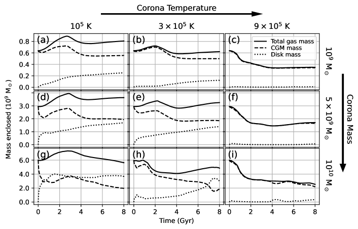
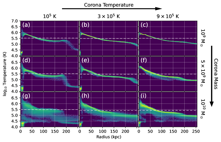
Figure 4: Magellanic Corona stability. Study of the stability of the Magellanic Corona for varying initial masses and temperatures. Each panel shows the total, CGM, and disk masses within 120 kpc as a function of time (solid, dashed, and dotted lines, respectively). The initial temperatures increase from left to right with values of 1, 3, and $9\times 10^{5}$ K. The initial masses increase from top to bottom with values of 1, 5, and $10\times 10^{9}$ $\mathrm{M}_{\odot}$ (within 200 kpc). Our fiducial model (see Section 4.3) is the center frame (Panel e) corresponding to an initial mass of $3\times 10^{9}$ $\mathrm{M}_{\odot}$ and a temperature of $3\times 10^{5}$ K.

Figure 5: Magellanic Corona temperature. Temperature profile of the Magellanic Corona for nine initial masses and temperatures (as in Figure 5). These histograms show the relative density of the gas temperature as a function of radius for the nine simulations at $t=4$ Gyr. The horizontal white dashed lines show the mean temperature of the gas within $20<r<250$ kpc.

Figure 5 shows these results. The nine panels depict nine different simulations with varying initial conditions in which the LMC and Magellanic Corona were evolved in isolation. The initial temperature of the Corona increases from left to right (with values of 1, 3, and $9\times 10^{5}$ K), while the initial mass of the Corona increases from top to bottom (1, 5, and $10\times 10^{9}$ $\mathrm{M}_{\odot}$ within 200 kpc). The black lines show the total masses of the gaseous components within 120 kpc (the virial radius of the LMC) as a function of time – total gas mass (solid), ionized mass (circumgalactic Coronal gas; dashed), and neutral disk mass (dotted).

Figure 5 also shows the temperature distribution as a function of radius for the nine simulations at $t=4$ Gyr. Again initial temperature increases to the right and the initial gas mass increases downwards. The mean temperature of the gas within $20<r<250$ kpc is shown as a horizontal dashed line. Interestingly, these white lines don’t vary dramatically between the three columns. This means that the initial temperature has a minimal, if any effect on the stable temperature of the Corona.

We do, however, see that increasing the initial mass of the Corona affects the spread in temperatures. We believe this is due to the fact that the Coronae with higher initial masses contain higher density gas which can cool more effectively. Cooling is very efficient around $10^{5}$ K, so subtle changes in density and temperature can have a strong impact on the strength of cooling. These higher density Coronae thus don’t have sufficient supernova energy injection to keep the gas warm.

4.2 Effect on the Magellanic Stream

We now want to explore the effect of varying the Magellanic Corona’s initial mass and temperature on the properties of the present-day Magellanic System. The initial total mass of the Corona directly affects the amount of ionized gas that we observe around the Stream today. Via absorption-line spectroscopy, Fox et al. (2014) estimated that there is $\sim 1.5\times 10^{9}$ $\mathrm{M}_{\odot}$ of ionized gas associated with the Magellanic System, $\sim 10^{9}$ $\mathrm{M}_{\odot}$ of which is in the Trailing Stream region. Figure 6 shows the total mass in the Trailing Stream for various different models. These values were calculated by mimicking the observational technique of integrating the column density at an assumed distance of 55 kpc. These are not the physical masses in the system (see Section 3.1), but allow us to compare directly with the observational estimates shown in the left-most bar (Brüns et al., 2005; Fox et al., 2014). Continuing from left to right we have the results from the simulations published in Besla et al. (2012) and Pardy et al. (2018) in which no ionized material was produced. The three right-most bars show the results of our simulations for three different initial Corona masses, 1, 5, and $10\times 10^{9}$ $\mathrm{M}_{\odot}$ (corresponding to Panels b, e, and h in Figures 5 and 5). Clearly, as we increase the progenitor mass, we are able to produce more ionized material in the Stream. For masses below $5\times 10^{9}$ $\mathrm{M}_{\odot}$ we are unable to reproduce the observations. In the models that we tested, either $5\times 10^{9}$ or $10^{10}$ $\mathrm{M}_{\odot}$ result in viable models. For masses larger than $10^{10}$ $\mathrm{M}_{\odot}$, the mass of the LMC’s CGM begins to approach estimates of the MW CGM’s mass. Given the significant difference in virial masses of the two galaxies, having similar coronal masses is unlikely. Therefore Magellanic Corona masses below $10^{10}$ $\mathrm{M}_{\odot}$ are preferred.

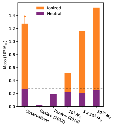
Figure 6: The mass of the Trailing Stream. Each bar shows the results for a different model compared against the observed mass in neutral and ionized gas shown in the left-most column ($2.7\times 10^{8}$ $\mathrm{M}_{\odot}$ in neutral gas, Brüns et al. 2005; $1.0\times 10^{9}$ $\mathrm{M}_{\odot}$ in ionized gas, though this may be an underestimate Fox et al. 2014). Each value is computed by integrating the column densities for all gas behind the SMC ($l_{\mathrm{MS}}<l_{\mathrm{MS,SMC}}$) assuming a distance to the gas of 55 kpc (as done in observational works, Brüns et al. 2005, Fox et al. 2014). The total neutral masses in Besla et al. (2012), and Pardy et al. (2018) are $2.5\times 10^{7}$ $\mathrm{M}_{\odot}$ and $1.9\times 10^{8}$ $\mathrm{M}_{\odot}$, respectively. The three right-most columns show the results from our new simulations with initial Magellanic Corona masses of 1, 5, and $10\times 10^{9}$ $\mathrm{M}_{\odot}$ (at a temperature of $3\times 10^{5}$ K; Panels b, e, and h in Figures 5 and 5). The neutral material is relatively consistent between these models at 2.2, 2.1, and $2.5\times 10^{8}$ $\mathrm{M}_{\odot}$, while the ionized gas masses are $3.0\times 10^{8}$, $9.5\times 10^{8}$, and $1.3\times 10^{9}$ $\mathrm{M}_{\odot}$ for the low, medium, and high mass models, respectively. By dividing the ionized mass by the total mass, we can get an approximate value for the average ionization fraction in the Magellanic Trailing Stream, and we find values of 57%, 82%, and 84% for the three models (compared with $\sim 75\%$ in the observed case).

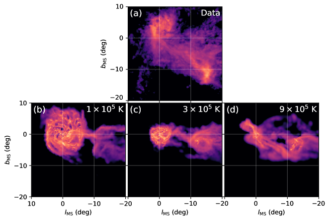
Figure 7: Present-day LMC disk for different Corona temperatures. A zoomed in region around the Magellanic Clouds is shown in Magellanic Coordinates for the observational data (Panel a; HI4PI, Westmeier 2018) compared with three different simulations (bottom panels). Panels b, c, and d show the results from initial Magellanic Corona temperatures of 1, 3, and $9\times 10^{5}$ K, respectively (with a total mass of $5\times 10^{9}$ $\mathrm{M}_{\odot}$; Panels d, e, and f in Figures 5 and 5). As the temperature decreases the size of the LMC disk increases due to Corona material collapsing onto the disk. At higher temperatures (Panel d), barely any LMC disk forms.

We also explored the impact of the initial Magellanic Corona temperature on the present-day Magellanic System. As shown in Figure 5, the initial temperature doesn’t have a large effect on the temperature distribution or on the mean Corona temperature after 4 Gyr of evolution. The main difference that we see between temperature models is in the properties of the LMC disk. Since we form our LMC disk self-consistently by letting it condense out of the Corona, the temperature plays a large role in its size and stability. Figure 7 shows the LMC’s disk at the present day for three different simulations compared with observational data from the HI4PI survey (HI4PI Collaboration et al., 2016; Westmeier, 2018). Panels a, b, and c show the results from simulations with initial Magellanic Corona Masses of 1, 3, and $9\times 10^{5}$ K, respectively. Lower initial Corona temperatures leads to larger LMC disks due to more material cooling and falling towards the center of the gravitational potential. For the highest temperatures (Panel c), no LMC disk forms since the Corona material can’t cool and fall to the center of the gravitational potential. This is also visible in Figure 5f in which the dotted line (showing the total disk mass) remains at zero throughout the simulation.

4.3 Fiducial Model

Based on these tests, our chosen fiducial Magellanic Corona was follows an isothermal profile with a total mass (within 200 kpc) of $5\times 10^{9}$ $\mathrm{M}_{\odot}$ and a temperature of $3\times 10^{5}$ K. We used an initial metallicity of 0.1 solar. After 3.5 Gyr in isolation, $3.7\times 10^{9}$ $\mathrm{M}_{\odot}$ of ionized material remains bound to the LMC (with $2\times 10^{9}$ $\mathrm{M}_{\odot}$ within 120 kpc) and its median temperature has risen to $3.4\times 10^{5}$ K. The LMC’s neutral gas disk has condensed out of the Corona with a mass of $9.1\times 10^{8}$ $\mathrm{M}_{\odot}$.

5 Discussion

The Magellanic Corona model of the evolution of the Magellanic System presented here is distinct from the historical dichotomy of Stream formation models: the tidal model (e.g. Fujimoto & Sofue, 1976; Besla et al., 2010, 2012; Pardy et al., 2018), and the ram-pressure model (e.g. Meurer et al., 1985; Hammer et al., 2015; Wang et al., 2019).

In modern first-infall tidal models (Besla et al., 2012), the Trailing Stream and Leading Arm are formed through 4 interactions over 7 Gyr, however no MW CGM was included. In response to the observations of the large ionized mass in the Stream (Fox et al., 2014), Pardy et al. (2018) attemped to increase the stripped material in the Magellanic System by increasing in the pre-infall LMC and SMC gaseous disk masses. While this brought the present-day neutral Stream mass closer to the observed values (see Figure 6), it wasn’t enough to account for the total mass of $>10^{9}$ $\mathrm{M}_{\odot}$. Winds and outflows from the LMC were also determined to be insufficient to supply the required gas mass into the Stream (Bustard et al., 2018, 2020).

Setton et al. (2023) explored the implications of the bow shock generated as the LMC approaches the MW. The envelope of shocked gas could possibly explain the ionized gas detections of Fox et al. (2014), however this isn’t explored in depth in their work. Our model presented here does produce some of the same bow shock features including a high temperature leading edge of ionized gas (visible in Panels b and e of Figure 3. Because of the inclusion of the Magellanic Corona in our models, there is less of a clear shock boundary, however we are still consistent with the observed H$\alpha$ emission and ionized gas properties.

The other proposed formation pathway for the Magellanic Stream involves ram-pressure stripping gas out of the LMC and SMC disks (Hammer et al., 2015; Wang et al., 2019). While this model is able to account for many of the features of the Magellanic System, including its turbulent morphology and ionized gas component, it requires a very low mass for the LMC ($<2\times 10^{10}$ $\mathrm{M}_{\odot}$) with little to no dark matter. This is in contrast with the many indirect indications of the LMC’s mass shown in Figure 1. Moreover, they use relatively low mass models of the MW while including a very extended, high-mass CGM (total masses of $\sim$7 and $8\times 10^{11}$ $\mathrm{M}_{\odot}$ with CGM masses of 2 and $1.5\times 10^{11}$ $\mathrm{M}_{\odot}$, i.e. 28% and 18%, respectively). These gaseous halos extend out beyond 500 kpc and we have not been able to reproduce the stability reported in Figure 1 of Wang et al. (2019). Finally, they do not discuss the metallicity along the length of the Stream which may not agree with observations given that there is significant LMC material stripped.

Our model now includes the Magellanic Corona which not only provides the bulk of the mass in the Magellanic System (in the form of warm ionized gas), but it, combined with the MW coronal gas, provides the required hydrodynamical forces to shape the Stream into its observed complex, turbulent morphology. We are now able to explain the total observed mass ($>10^{9}$ $\mathrm{M}_{\odot}$), the high ionization fraction ($>75\%$), the filamentary structure of the Trailing Stream, and the behavior of the metals.

Due to the tidal interactions between the Clouds in our model, we still predict a $>30$ mag arcsec^-2 stellar stream as in previous models (Pardy et al. 2018; L21). These stars which are stripped out of the disk of the SMC lie up to 20^∘ offset from the gaseous Stream in Magellanic Latitude and are at distances ranging from 10 kpc to $>100$ kpc with a median distance of $42$ kpc. Despite extensive work looking to detect the stellar counterpart to the Magellanic Stream, only a few candidates have emerged. Zaritsky et al. (2020) found 15 stars near the tip of the Stream at distances of $40-80$ kpc with metallicities and velocities consistent with the SMC. More recently, Chandra et al. (2023) found 13 stars with kinematics matching the Clouds that lie at distances of $60-100$ kpc, however this study only explored stars beyond 50 kpc. Our model presented here can reproduce the Zaritsky et al. (2020) stars, however the Chandra et al. (2023) stars are at too large of a distance to be directly reproduced in this model. This could be resolved by including a stellar halo around either Cloud which could contribute to these few metal-poor stars at very high distances even if the bulk of the Stream (gaseous and stellar) is nearby.

As discussed in L21, the Leading Arm may not be Magellanic material. While H I observations linked the leading gas clumps with the LMC and SMC based on their high velocities and spatial locations (Putman et al., 1998), UV spectroscopy has shown the Leading Arm contains a range of metallicities (Fox et al., 2018; Richter et al., 2018) and complex kinematics (Fox et al., 2020), casting doubt on its origin. Due to the existence of a “Magellanic Group” of galaxies that approached the MW together with the Clouds (D’Onghia & Lake, 2008; Nichols et al., 2011; Sales et al., 2011, 2017; Bechtol et al., 2015; Jahn et al., 2019; Pardy et al., 2020; Santos-Santos et al., 2021), the Leading Arm material could have been ram-pressure stripped off of a forerunner satellite that fell into the MW ahead of the LMC and SMC (Yang et al., 2014; Tepper-García et al., 2015). However, candidate satellites with the correct positions and velocities have not yet been identified (Tepper-García et al., 2019). In our exploration of orbital parameters, we have found orbits in which material is stripped out ahead of the Clouds, however the Trailing Stream is not very well reproduced in these models. In future work, we will better explore this orbital parameter space in addition to reinvestigating the observations of the Leading Arm to constrain its origin.

5.1 Constraining the Milky Way Corona

By exploring the parameter space of temperatures and densities for the MW’s own hot gas corona, we can isolate its effects on the formation and morphology of the Trailing Stream. In this way, we can constrain the CGM properties by comparing our simulations with observations. Inspired by observations (e.g. Anderson & Bregman, 2010; Bregman et al., 2018), we varied the total mass from $10^{10}$ to $8\times 10^{10}$ $\mathrm{M}_{\odot}$, varied the temperature from $4\times 10^{5}$ to $3\times 10^{6}$ K, and tested with and without uniform rotation of the CGM. As we found above with the Magellanic Corona, changing the initial temperature of the gas did not affect the equilibrium temperature distribution significantly. Similarly, rotation, while it did decrease the equilibrium temperature of the CGM slightly, did not have a substantial effect on the Magellanic System. Therefore, the main variable we explored was the total mass.

L21 found that a MW corona mass of $4\times 10^{10}$ $\mathrm{M}_{\odot}$ was required to get the best match to the velocity gradient along the Stream (two times larger than Salem et al. 2015). In the suite of orbits tested in this paper, we found that the largest effect that the MW corona had on the present-day Stream is on the morphology of the neutral and ionized components. Figure 8 shows the ionized (orange) and neutral (grayscale contours) components of the simulated Streams in Magellanic Coordinates for three different models. The total mass of the MW corona increases from top to bottom with values of 1, 2, and $8\times 10^{10}$ $\mathrm{M}_{\odot}$. The higher gas density induces stronger ram pressure on the Magellanic gas, decreasing the on-sky extent of the ionized gas, and making the neutral Stream longer and narrower. We find that a value of $2\times 10^{10}$ $\mathrm{M}_{\odot}$ (Panel b; in agreement with estimates from Salem et al. 2015) provides the best agreement with the observations.

This led to our fiducial MW corona model with a total mass of $2\times 10^{10}$ $\mathrm{M}_{\odot}$ and a temperature of $10^{6}$ K. After 2 Gyr of evolution in isolation, $1.9\times 10^{10}$ $\mathrm{M}_{\odot}$ remains bound to the MW and the coronal gas has a mean temperature of $1.4\times 10^{6}$ K.

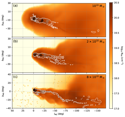
Figure 8: The Effect of the MW Corona on the Present-Day Stream. The ionized (orange) and neutral (grayscale contours) Magellanic gas for three simulations shown as they would appear on the sky in Magellanic Coordinates. Panels a, b, and c, show the results of simulations with a total MW coronal mass of 1, 2, and $8\times 10^{10}$ $\mathrm{M}_{\odot}$, respectively (listed in the top right of each panel). All panels use our fiducial LMC with a Magellanic Corona of $5\times 10^{9}$ $\mathrm{M}_{\odot}$ at $3\times 10^{5}$ K. The neutral gas contours (white, grey, and black) are at values of log${}_{10}(N_{\mathrm{HI}})=19$, 20, and 21, respectively.

6 Conclusions

Building on our earlier work (; ), we have characterized the influence of the Magellanic Corona on the formation and evolution of the Magellanic Stream. With this suite of simulations, we have shown that the first-infall Magellanic Corona model of Stream formation can produce a present-day Magellanic System with properties in agreement with the observations (Figure 3). The ionized component is formed out of the Magellanic Corona, which becomes warped and shaped around the Clouds and the neutral Stream through its interactions with the MW’s own hot coronal gas. The trailing Stream’s turbulent morphology seen in H I is reproduced through interactions between the neutral gas and the warm/hot gas in the Magellanic and Galactic Coronae. We find metal distributions and ionization fractions in agreement with absorption-line spectroscopy observations.

We have also explored the parameter space of temperatures and densities for the Magellanic Corona to constrain its properties. We find that a mass $>5\times 10^{9}$ $\mathrm{M}_{\odot}$ (within 200 kpc) can provide sufficient ionized material at the present day (Figure 6). By forming the LMC’s gaseous disk self-consistently out of the Corona, we are able to reproduce the gas mass within the galaxy’s disk at the present day. The initial temperature of the Coronal gas determines the size and mass of the LMC’s disk at later times, so we found that a value of $3\times 10^{5}$ K (in agreement with the virial temperature) provides the best results (Figure 7).

These models show that we are able to reproduce the properties of observed Magellanic System while accounting for a large LMC mass. The Magellanic Corona provides the key element that necessitates a review of the precise orbital histories of the Clouds. This brings the Trailing Stream gas much closer to us than previously thought, explaining the turbulent morphology and H $\alpha$ brightness, and implying an infall onto the MW disk within $\sim$100 Myr.

By obtaining constraints on the distance to the gas in the Stream through absorption-line spectroscopy towards MW halo stars, we will be able to better discriminate between existing models. Moreover, a reevaluation of the properties of the Leading Arm could lead to answers on whether it is of Magellanic origin or not. These observations and more will constrain key properties of the Magellanic System, giving us the information we need to converge on the true history of the Magellanic Clouds.

References

- Anderson & Bregman (2010) Anderson, M. E., & Bregman, J. N. 2010, ApJ, 714, 320, doi: 10.1088/0004-637X/714/1/320
- Astropy Collaboration et al. (2013) Astropy Collaboration, Robitaille, T. P., Tollerud, E. J., et al. 2013, A&A, 558, A33, doi: 10.1051/0004-6361/201322068
- Astropy Collaboration et al. (2018) Astropy Collaboration, Price-Whelan, A. M., Sipőcz, B. M., et al. 2018, AJ, 156, 123, doi: 10.3847/1538-3881/aabc4f
- Astropy Collaboration et al. (2022) Astropy Collaboration, Price-Whelan, A. M., Lim, P. L., et al. 2022, apj, 935, 167, doi: 10.3847/1538-4357/ac7c74
- Barger et al. (2017) Barger, K. A., Madsen, G. J., Fox, A. J., et al. 2017, ApJ, 851, 110, doi: 10.3847/1538-4357/aa992a
- Bechtol et al. (2015) Bechtol, K., Drlica-Wagner, A., Balbinot, E., et al. 2015, ApJ, 807, 50, doi: 10.1088/0004-637X/807/1/50
- Besla et al. (2007) Besla, G., Kallivayalil, N., Hernquist, L., et al. 2007, ApJ, 668, 949, doi: 10.1086/521385
- Besla et al. (2010) —. 2010, ApJ, 721, L97, doi: 10.1088/2041-8205/721/2/L97
- Besla et al. (2012) —. 2012, MNRAS, 421, 2109, doi: 10.1111/j.1365-2966.2012.20466.x
- Bland-Hawthorn et al. (2013) Bland-Hawthorn, J., Maloney, P. R., Sutherland, R. S., & Madsen, G. J. 2013, ApJ, 778, 58, doi: 10.1088/0004-637X/778/1/58
- Bland-Hawthorn et al. (2019) Bland-Hawthorn, J., Maloney, P. R., Sutherland, R., et al. 2019, ApJ, 886, 45, doi: 10.3847/1538-4357/ab44c8
- Bregman et al. (2018) Bregman, J. N., Anderson, M. E., Miller, M. J., et al. 2018, ApJ, 862, 3, doi: 10.3847/1538-4357/aacafe
- Brüns et al. (2005) Brüns, C., Kerp, J., Staveley-Smith, L., et al. 2005, A&A, 432, 45, doi: 10.1051/0004-6361:20040321
- Bustard & Gronke (2022) Bustard, C., & Gronke, M. 2022, ApJ, 933, 120, doi: 10.3847/1538-4357/ac752b
- Bustard et al. (2018) Bustard, C., Pardy, S. A., D’Onghia, E., Zweibel, E. G., & Gallagher, J. S., I. 2018, ApJ, 863, 49, doi: 10.3847/1538-4357/aad08f
- Bustard et al. (2020) Bustard, C., Zweibel, E. G., D’Onghia, E., Gallagher, J. S., I., & Farber, R. 2020, ApJ, 893, 29, doi: 10.3847/1538-4357/ab7fa3
- Center for High Throughput Computing (2006) Center for High Throughput Computing. 2006, Center for High Throughput Computing, Center for High Throughput Computing, doi: 10.21231/GNT1-HW21
- Chandra et al. (2023) Chandra, V., Naidu, R. P., Conroy, C., et al. 2023, ApJ, 956, 110, doi: 10.3847/1538-4357/acf7bf
- Cioni et al. (2000) Cioni, M. R. L., Habing, H. J., & Israel, F. P. 2000, A&A, 358, L9, doi: 10.48550/arXiv.astro-ph/0005057
- Cohen (1982) Cohen, R. J. 1982, MNRAS, 199, 281, doi: 10.1093/mnras/199.2.281
- Connors et al. (2006) Connors, T. W., Kawata, D., & Gibson, B. K. 2006, MNRAS, 371, 108, doi: 10.1111/j.1365-2966.2006.10659.x
- Davies & Wright (1977) Davies, R. D., & Wright, A. E. 1977, MNRAS, 180, 71, doi: 10.1093/mnras/180.2.71
- De Leo et al. (2020) De Leo, M., Carrera, R., Noël, N. E. D., et al. 2020, MNRAS, 495, 98, doi: 10.1093/mnras/staa1122
- Di Teodoro et al. (2019) Di Teodoro, E. M., McClure-Griffiths, N. M., Jameson, K. E., et al. 2019, MNRAS, 483, 392, doi: 10.1093/mnras/sty3095
- Diaz & Bekki (2011) Diaz, J., & Bekki, K. 2011, MNRAS, 413, 2015, doi: 10.1111/j.1365-2966.2011.18289.x
- D’Onghia & Fox (2016) D’Onghia, E., & Fox, A. J. 2016, ARA&A, 54, 363, doi: 10.1146/annurev-astro-081915-023251
- D’Onghia & Lake (2008) D’Onghia, E., & Lake, G. 2008, ApJ, 686, L61, doi: 10.1086/592995
- Erkal & Belokurov (2020) Erkal, D., & Belokurov, V. A. 2020, MNRAS, 495, 2554, doi: 10.1093/mnras/staa1238
- Erkal et al. (2019) Erkal, D., Belokurov, V., Laporte, C. F. P., et al. 2019, MNRAS, 487, 2685, doi: 10.1093/mnras/stz1371
- For et al. (2014) For, B.-Q., Staveley-Smith, L., Matthews, D., & McClure-Griffiths, N. M. 2014, ApJ, 792, 43, doi: 10.1088/0004-637X/792/1/43
- Fox et al. (2020) Fox, A. J., Frazer, E. M., Bland-Hawthorn, J., et al. 2020, ApJ, 897, 23, doi: 10.3847/1538-4357/ab92a3
- Fox et al. (2013) Fox, A. J., Richter, P., Wakker, B. P., et al. 2013, ApJ, 772, 110, doi: 10.1088/0004-637X/772/2/110
- Fox et al. (2010) Fox, A. J., Wakker, B. P., Smoker, J. V., et al. 2010, ApJ, 718, 1046, doi: 10.1088/0004-637X/718/2/1046
- Fox et al. (2014) Fox, A. J., Wakker, B. P., Barger, K. A., et al. 2014, ApJ, 787, 147, doi: 10.1088/0004-637X/787/2/147
- Fox et al. (2018) Fox, A. J., Barger, K. A., Wakker, B. P., et al. 2018, ApJ, 854, 142, doi: 10.3847/1538-4357/aaa9bb
- Fujimoto & Sofue (1976) Fujimoto, M., & Sofue, Y. 1976, A&A, 47, 263
- Gardiner & Noguchi (1996) Gardiner, L. T., & Noguchi, M. 1996, MNRAS, 278, 191, doi: 10.1093/mnras/278.1.191
- Gibson et al. (2000) Gibson, B. K., Giroux, M. L., Penton, S. V., et al. 2000, AJ, 120, 1830, doi: 10.1086/301545
- Graczyk et al. (2020) Graczyk, D., Pietrzyński, G., Thompson, I. B., et al. 2020, ApJ, 904, 13, doi: 10.3847/1538-4357/abbb2b
- Hammer et al. (2015) Hammer, F., Yang, Y. B., Flores, H., Puech, M., & Fouquet, S. 2015, ApJ, 813, 110, doi: 10.1088/0004-637X/813/2/110
- HI4PI Collaboration et al. (2016) HI4PI Collaboration, Ben Bekhti, N., Flöer, L., et al. 2016, A&A, 594, A116, doi: 10.1051/0004-6361/201629178
- Hopkins (2015) Hopkins, P. F. 2015, MNRAS, 450, 53, doi: 10.1093/mnras/stv195
- Hopkins et al. (2013) Hopkins, P. F., Narayanan, D., & Murray, N. 2013, MNRAS, 432, 2647, doi: 10.1093/mnras/stt723
- Hopkins et al. (2018) Hopkins, P. F., Wetzel, A., Kereš, D., et al. 2018, MNRAS, 480, 800, doi: 10.1093/mnras/sty1690
- Hummels et al. (2017) Hummels, C. B., Smith, B. D., & Silvia, D. W. 2017, ApJ, 847, 59, doi: 10.3847/1538-4357/aa7e2d
- Jahn et al. (2019) Jahn, E. D., Sales, L. V., Wetzel, A., et al. 2019, MNRAS, 489, 5348, doi: 10.1093/mnras/stz2457
- Jahn et al. (2021) —. 2021, arXiv e-prints, arXiv:2106.03861. https://arxiv.org/abs/2106.03861
- Kallivayalil et al. (2006) Kallivayalil, N., van der Marel, R. P., Alcock, C., et al. 2006, ApJ, 638, 772, doi: 10.1086/498972
- Kallivayalil et al. (2013) Kallivayalil, N., van der Marel, R. P., Besla, G., Anderson, J., & Alcock, C. 2013, ApJ, 764, 161, doi: 10.1088/0004-637X/764/2/161
- Kim et al. (2016) Kim, J.-h., Agertz, O., Teyssier, R., et al. 2016, ApJ, 833, 202, doi: 10.3847/1538-4357/833/2/202
- Koposov et al. (2023) Koposov, S. E., Erkal, D., Li, T. S., et al. 2023, MNRAS, doi: 10.1093/mnras/stad551
- Krishnarao et al. (2022) Krishnarao, D., Fox, A. J., D’Onghia, E., et al. 2022, Nature, 609, 915, doi: 10.1038/s41586-022-05090-5
- Lin & Lynden-Bell (1977) Lin, D. N. C., & Lynden-Bell, D. 1977, MNRAS, 181, 59, doi: 10.1093/mnras/181.2.59
- Lin & Lynden-Bell (1982) —. 1982, MNRAS, 198, 707, doi: 10.1093/mnras/198.3.707
- Lu et al. (1994) Lu, L., Savage, B. D., & Sembach, K. R. 1994, ApJ Letters, 437, L119, doi: 10.1086/187697
- Lucchini et al. (2021) Lucchini, S., D’Onghia, E., & Fox, A. J. 2021, ApJ Letters, 921, L36, doi: 10.3847/2041-8213/ac3338
- Lucchini et al. (2020) Lucchini, S., D’Onghia, E., Fox, A. J., et al. 2020, Nature, 585, 203, doi: 10.1038/s41586-020-2663-4
- Mathewson et al. (1974) Mathewson, D. S., Cleary, M. N., & Murray, J. D. 1974, ApJ, 190, 291, doi: 10.1086/152875
- Meurer et al. (1985) Meurer, G. R., Bicknell, G. V., & Gingold, R. A. 1985, PASA, 6, 195, doi: 10.1017/S1323358000018075
- Moore & Davis (1994) Moore, B., & Davis, M. 1994, MNRAS, 270, 209, doi: 10.1093/mnras/270.2.209
- Morras (1983) Morras, R. 1983, AJ, 88, 62, doi: 10.1086/113287
- Murray et al. (2019) Murray, C. E., Peek, J. E. G., Di Teodoro, E. M., et al. 2019, ApJ, 887, 267, doi: 10.3847/1538-4357/ab510f
- Nichols et al. (2011) Nichols, M., Colless, J., Colless, M., & Bland-Hawthorn, J. 2011, ApJ, 742, 110, doi: 10.1088/0004-637X/742/2/110
- Nidever et al. (2008) Nidever, D. L., Majewski, S. R., & Butler Burton, W. 2008, ApJ, 679, 432, doi: 10.1086/587042
- Nidever et al. (2010) Nidever, D. L., Majewski, S. R., Butler Burton, W., & Nigra, L. 2010, ApJ, 723, 1618, doi: 10.1088/0004-637X/723/2/1618
- Pardy et al. (2018) Pardy, S. A., D’Onghia, E., & Fox, A. J. 2018, ApJ, 857, 101, doi: 10.3847/1538-4357/aab95b
- Pardy et al. (2020) Pardy, S. A., D’Onghia, E., Navarro, J. F., et al. 2020, MNRAS, 492, 1543, doi: 10.1093/mnras/stz3192
- Peñarrubia et al. (2016) Peñarrubia, J., Gómez, F. A., Besla, G., Erkal, D., & Ma, Y.-Z. 2016, MNRAS, 456, L54, doi: 10.1093/mnrasl/slv160
- Perret et al. (2014) Perret, V., Renaud, F., Epinat, B., et al. 2014, A&A, 562, A1, doi: 10.1051/0004-6361/201322395
- Petersen & Peñarrubia (2021) Petersen, M. S., & Peñarrubia, J. 2021, Nature Astronomy, 5, 251, doi: 10.1038/s41550-020-01254-3
- Price-Whelan et al. (2022) Price-Whelan, A., Sipőcz, B., Lenz, D., et al. 2022, adrn/gala: v1.6.1, v1.6.1, Zenodo, doi: 10.5281/zenodo.7299506
- Price-Whelan (2017) Price-Whelan, A. M. 2017, The Journal of Open Source Software, 2, doi: 10.21105/joss.00388
- Putman et al. (2003) Putman, M. E., Staveley-Smith, L., Freeman, K. C., Gibson, B. K., & Barnes, D. G. 2003, ApJ, 586, 170, doi: 10.1086/344477
- Putman et al. (1998) Putman, M. E., Gibson, B. K., Staveley-Smith, L., et al. 1998, Nature, 394, 752, doi: 10.1038/29466
- Read & Erkal (2019) Read, J. I., & Erkal, D. 2019, MNRAS, 487, 5799, doi: 10.1093/mnras/stz1320
- Richter et al. (2018) Richter, P., Fox, A. J., Wakker, B. P., et al. 2018, ApJ, 865, 145, doi: 10.3847/1538-4357/aadd0f
- Richter et al. (2013) —. 2013, ApJ, 772, 111, doi: 10.1088/0004-637X/772/2/111
- Röttgers (2018) Röttgers, B. 2018, pygad: Analyzing Gadget Simulations with Python, Astrophysics Source Code Library, record ascl:1811.014. http://ascl.net/1811.014
- Röttgers et al. (2020) Röttgers, B., Naab, T., Cernetic, M., et al. 2020, MNRAS, 496, 152, doi: 10.1093/mnras/staa1490
- Salem et al. (2015) Salem, M., Besla, G., Bryan, G., et al. 2015, ApJ, 815, 77, doi: 10.1088/0004-637X/815/1/77
- Sales et al. (2011) Sales, L. V., Navarro, J. F., Cooper, A. P., et al. 2011, MNRAS, 418, 648, doi: 10.1111/j.1365-2966.2011.19514.x
- Sales et al. (2017) Sales, L. V., Navarro, J. F., Kallivayalil, N., & Frenk, C. S. 2017, MNRAS, 465, 1879, doi: 10.1093/mnras/stw2816
- Santos-Santos et al. (2021) Santos-Santos, I. M. E., Fattahi, A., Sales, L. V., & Navarro, J. F. 2021, MNRAS, 504, 4551, doi: 10.1093/mnras/stab1020
- Sembach et al. (2003) Sembach, K. R., Wakker, B. P., Savage, B. D., et al. 2003, ApJ Supplement, 146, 165, doi: 10.1086/346231
- Setton et al. (2023) Setton, D. J., Besla, G., Patel, E., et al. 2023, arXiv e-prints, arXiv:2308.10963, doi: 10.48550/arXiv.2308.10963
- Shipp et al. (2021) Shipp, N., Erkal, D., Drlica-Wagner, A., et al. 2021, ApJ, 923, 149, doi: 10.3847/1538-4357/ac2e93
- Sofue (1994) Sofue, Y. 1994, PASJ, 46, 431, doi: 10.48550/arXiv.astro-ph/9403041
- Springel (2005) Springel, V. 2005, MNRAS, 364, 1105, doi: 10.1111/j.1365-2966.2005.09655.x
- Springel & Hernquist (2003) Springel, V., & Hernquist, L. 2003, MNRAS, 339, 289, doi: 10.1046/j.1365-8711.2003.06206.x
- Stanimirović et al. (2004) Stanimirović, S., Staveley-Smith, L., & Jones, P. A. 2004, ApJ, 604, 176, doi: 10.1086/381869
- Subramanian & Subramaniam (2012) Subramanian, S., & Subramaniam, A. 2012, ApJ, 744, 128, doi: 10.1088/0004-637X/744/2/128
- Tepper-García et al. (2019) Tepper-García, T., Bland-Hawthorn, J., Pawlowski, M. S., & Fritz, T. K. 2019, MNRAS, 488, 918, doi: 10.1093/mnras/stz1659
- Tepper-García et al. (2015) Tepper-García, T., Bland-Hawthorn, J., & Sutherland , R. S. 2015, ApJ, 813, 94, doi: 10.1088/0004-637X/813/2/94
- van der Marel & Kallivayalil (2014) van der Marel, R. P., & Kallivayalil, N. 2014, ApJ, 781, 121, doi: 10.1088/0004-637X/781/2/121
- Vasiliev (2024) Vasiliev, E. 2024, MNRAS, 527, 437, doi: 10.1093/mnras/stad2612
- Vasiliev et al. (2021) Vasiliev, E., Belokurov, V., & Erkal, D. 2021, MNRAS, 501, 2279, doi: 10.1093/mnras/staa3673
- Wan et al. (2020) Wan, Z., Guglielmo, M., Lewis, G. F., Mackey, D., & Ibata, R. A. 2020, MNRAS, 492, 782, doi: 10.1093/mnras/stz3493
- Wang et al. (2019) Wang, J., Hammer, F., Yang, Y., et al. 2019, MNRAS, 486, 5907, doi: 10.1093/mnras/stz1274
- Westmeier (2018) Westmeier, T. 2018, MNRAS, 474, 289, doi: 10.1093/mnras/stx2757
- Wiersma et al. (2009) Wiersma, R. P. C., Schaye, J., & Smith, B. D. 2009, MNRAS, 393, 99, doi: 10.1111/j.1365-2966.2008.14191.x
- Wolfire et al. (1995) Wolfire, M. G., McKee, C. F., Hollenbach, D., & Tielens, A. G. G. M. 1995, ApJ, 453, 673, doi: 10.1086/176429
- Yang et al. (2014) Yang, Y., Hammer, F., Fouquet, S., et al. 2014, MNRAS, 442, 2419, doi: 10.1093/mnras/stu931
- Zaritsky et al. (2000) Zaritsky, D., Harris, J., Grebel, E. K., & Thompson, I. B. 2000, ApJ Letters, 534, L53, doi: 10.1086/312649
- Zaritsky et al. (2020) Zaritsky, D., Conroy, C., Naidu, R. P., et al. 2020, ApJ Letters, 905, L3, doi: 10.3847/2041-8213/abcb83