Region analysis of QED massive fermion form factor

Abstract

We perform an analysis of the one- and two-loop massive quark form factor in QED in a region expansion, up to next-to-leading power in the quark mass. This yields an extensive set of regional integrals, categorized into three topologies, against which factorization theorems at next-to-leading power could be tested. Our analysis reveals a number of subtle aspects involving rapidity regulators, as well as additional regions that manifest themselves only beyond one loop, at the level of single diagrams, but which cancel in the form factor.

1 Introduction

The study of power corrections in scattering processes at hadron colliders has received increasing attention in the past few years due to its importance for precision physics. Power corrections become relevant every time a scattering process involves two, or more, widely separated scales. This is a very common situation at hadron colliders: different scales arise not only due to the presence of particles with very different masses. Often, different scales have a dynamical origin, related to the physical cuts necessary to select a given observable, or follow from the value of kinematic observables. Consider for instance a $n$-particle scattering process in QED, with the emission of an additional soft photon with momentum $k$, and denote the corresponding amplitude ${\cal M}_{n+1}$. This kinematic configuration is typical of processes occurring near threshold, where almost all the energy of the initial state particles goes into the required final state, such that extra radiation is constrained to be soft. The amplitude is conveniently described as a power expansion in the ratio $\xi\sim E/Q\ll 1$, where $E$ represents the energy of the soft photon, and $Q$ is the invariant mass of the final state

$${\cal M}_{n+1}={\cal M}^{\rm LP}_{n+1}+{\cal M}^{\rm NLP}_{n+1}+{\cal O}(\xi)\,,$$ (1)

where the leading power (LP) term scales as ${\cal M}^{\rm LP}_{n+1}\sim 1/\xi$, and the next-to-leading power (NLP) contribution is of order ${\cal M}^{\rm NLP}_{n+1}\sim\xi^{0}$. In perturbation theory each coefficient of the power expansion contains large logarithms of the type $\alpha_{s}^{n}\log^{m}\xi\sim 1$, with $m$ up to $2n-1$, which need to be resummed to obtain precise predictions.

Key to the resummation program is the determination of how the scattering amplitude factorizes into simpler (single scale) objects, involving the corresponding non-radiative amplitude ${\cal M}_{n}$ as well as collinear and soft matrix elements describing soft and collinear radiation. Factorization analyses can be developed within the original theory (i.e., QED or QCD), see e.g. Sterman:1987aj ; Catani:1989ne ; Catani:1990rp ; Korchemsky:1993xv ; Korchemsky:1993uz for seminal papers. Alternatively this can be done by means of an effective theory, such as the soft-collinear effective field theory (SCET) Bauer:2000yr ; Bauer:2001yt ; Beneke:2002ph , constructed to correctly reproduce soft and collinear modes in the scattering process. The factorization structure of the LP amplitude in Eq. (1) has been known for a long time, while the study of ${\cal M}^{\rm NLP}_{n+1}$ is more recent. Within QCD, factorization theorems have been developed for specific cases, such as the case $n=2$ corresponding to Drell-Yan like processes DelDuca:1990gz ; Bonocore:2016awd (see also Qiu:1990xxa ; Qiu:1990xy for factorization studies at NLP in $\Lambda^{2}_{\rm QCD}/Q^{2}$); the study of ${\cal M}^{\rm NLP}_{n+1}$ for general $n$ has been initiated in Laenen:2020nrt (see also Gervais:2017yxv ). Within SCET we refer to Beneke:2019oqx for studies of the factorization structure of Drell-Yan at general subleading power, and to Larkoski:2014bxa ; Beneke:2017ztn ; Beneke:2018rbh ; Beneke:2019kgv for various aspects of the factorization properties of the scattering amplitude ${\cal M}^{\rm NLP}_{n+1}$.

As discussed in Laenen:2020nrt , when studying the factorization of ${\cal M}^{\rm NLP}_{n+1}$, it is useful to distinguish two contributions: one in which the radiation is emitted from the external legs, and another in which the radiation is emitted internally, from a particle within the hard scattering kernel. Schematically, this corresponds to separating the amplitude into two parts

$${\cal M}_{n+1}={\cal M}_{n+1}^{\rm ext}+{\cal M}_{n+1}^{\rm int}\,.$$ (2)

This decomposition is useful, because the amplitude ${\cal M}_{n+1}^{\rm int}$ can actually be obtained by means of the Ward identity from ${\cal M}_{n+1}^{\rm ext}$. In turn, it was shown that understanding the factorization properties of ${\cal M}_{n+1}^{\rm ext}$ requires one to understand the factorization properties of the corresponding non-radiative amplitude, ${\cal M}_{n}$. This is best seen by considering for instance a soft photon emission from an outgoing fermion $i$. In this case ${\cal M}_{n+1}^{\rm ext}$ takes the form

$${\cal M}_{n+1}^{\rm ext}=\bar{u}(p_{i})(ieq_{i}\gamma^{\mu})\,\frac{i(\not{p}_{i}+\not{k}+m)}{(p_{i}+k)^{2}-m^{2}}\,{\cal M}_{n}(p_{1},\ldots,p_{i}+k,\ldots p_{n})\,,$$ (3)

where ${\cal M}_{n}$ represents the elastic amplitude (with the spinor $\bar{u}(p_{i})$ stripped off). Understanding the factorization of ${\cal M}_{n+1}^{\rm ext}$ requires the expansion of the non-radiative amplitude ${\cal M}_{n}$ for small $k$, but such expansion become non-trivial in presence of massless external particles, or external particles whose mass $m$ is much smaller compared to the other momentum invariants in the scattering, $m^{2}\ll s_{ij}$ with $s_{ij}=(p_{i}+p_{j})^{2}$. In this case, one needs to take into account that the non-radiative amplitude factorizes into non-trivial functions involving configurations of virtual soft and collinear momenta. According to the power counting analysis developed in Laenen:2020nrt , focusing only on the configurations which involve non-trivial collinear matrix elements, up to NLP the elastic amplitude factorizes according to

$$\mathcal{M}_{n}\big{|}^{\rm LP+NLP}_{\rm coll} =\bigg{(}\prod_{i=1}^{n}J_{(f)}^{i}\bigg{)}\otimes H\,S+\sum_{i=1}^{n}\bigg{(}\prod_{j\neq i}J_{(f)}^{j}\bigg{)}\Big{[}J^{i}_{(f\gamma)}\otimes H^{i}_{(f\gamma)}+J^{i}_{(f\partial\gamma)}\otimes H^{i}_{(f\partial\gamma)}\Big{]}\,S$$

$$\quad+\sum_{i=1}^{n}\bigg{(}\prod_{j\neq i}J_{(f)}^{j}\bigg{)}J^{i}_{(f\gamma\gamma)}\otimes H^{i}_{(f\gamma\gamma)}\,S+\sum_{i=1}^{n}\bigg{(}\prod_{j\neq i}J_{(f)}^{j}\bigg{)}J^{i}_{(f\!f\!f)}\otimes H^{i}_{(f\!f\!f)}\,S$$

$$\quad+\sum_{1\leq i\leq j\leq n}\bigg{(}\prod_{k\neq i,j}J_{(f)}^{k}\bigg{)}J^{i}_{(f\gamma)}J^{j}_{(f\gamma)}\otimes H^{ij}_{(f\gamma)(f\gamma)}\,S\,,$$ (4)

where the functions $J_{I}$ and $S$ describe long-distance collinear and soft virtual radiation in ${\cal M}_{n}$, and $H_{I}$ are hard functions, representing the contribution due to hard momenta configurations. In Eq. (1) the first term represents the LP contribution, while the second term in the first line starts at “$\sqrt{\rm NLP}$”, and the contributions in the second and third line start at NLP. Eq. (1) is expected to be valid to all orders in perturbation theory. In Laenen:2020nrt some explicit checks have been provided at one loop, however, a more thorough test of the factorization formula requires at least a two-loop computation, since the functions in the second and third lines of Eq. (1) appear for the first time at NNLO.

The purpose of this paper is to provide data that can be used to validate Eq. (1). To this end we consider the simplest QED process that gives non-trivial contributions to all the jet functions appearing in Eq. (1), namely, the annihilation of a massive fermion anti-fermion pair of mass $m$ into an off-shell photon of invariant mass $Q$ (or the time-reversed process of photon decay). More specifically, we consider the matrix element of the QED massive vector current $\bar{\psi}\gamma^{\mu}\psi$, which in turn is expressed in terms of two form factors $F_{1}(Q^{2},m^{2})$ and $F_{2}(Q^{2},m^{2})$. The two-loop result is known Bernreuther:2004ih ; Gluza:2009yy , and in recent years a lot of effort has been devoted to the calculation of the three loop correction Henn:2016kjz ; Henn:2016tyf ; Ablinger:2017hst ; Lee:2018nxa ; Lee:2018rgs ; Ablinger:2018yae ; Blumlein:2018tmz ; Blumlein:2019oas ; Fael:2022rgm ; Fael:2022miw ; Fael:2023zqr ; Blumlein:2023uuq , although no complete analytic result as yet exists.

For our purposes we need the two-loop small mass expansion of the form factors, i.e. $m\ll Q$, which is also given in Bernreuther:2004ih ; Gluza:2009yy . However, the small mass expansion alone does not provide enough information to compare with the corresponding factorized expression that one would obtain evaluating the form factor according to Eq. (1). Indeed, in the small mass limit it is possible to calculate the form factors with the method of expansion by momentum regions, Beneke:1997zp ; Smirnov:2002pj . Within this approach, one assigns to the loop momentum a specific scaling, which can be hard, collinear, soft, etc, with respect to the scaling of the external particle momenta. Each term defines a momentum region, and it is then possible to expand the form factors directly at the level of the integrand in the small parameters appearing in each region. The full result is recovered by summing over all regions. This approach is particularly useful because we expect the jet functions in Eq. (1) to be directly related with the collinear and anti-collinear region contributions.

To this end, we present in this paper the calculation of the two-loop massive form factors evaluated within the method of regions. To the best of our knowledge this is the first time that the two-loop result is evaluated entirely within this method. Thus far in literature only single integrals involved in the two-loop massive form factors have been evaluated within the method of regions, see e.g. Smirnov:1998vk ; Smirnov:1999bza ; Smirnov:2002pj . Besides providing more data for the comparison with Eq. (1) (which will be considered in a forthcoming work), this calculation actually has intrinsic value of its own.

For instance, one feature of the region expansion, which was found in Smirnov:1998vk ; Smirnov:1999bza ; Smirnov:2002pj , is that, at the level of single integrals, more regions appear at two loop, that were not present in the calculation at one loop. This is problematic from the point of view of an effective field theory description, and in general for the derivation of factorization theorems valid at all orders in perturbation theory. It is clear that if new momentum modes appear at each order in perturbation theory, no factorization theorem can be expected to be valid to all orders in perturbation theory. However, it was already observed in Becher:2007cu that, although new regions appear in single integrals at two loops, their contribution cancels when summing all diagrams, i.e. at the level of the form factors. The analysis in Becher:2007cu considered only the LP terms in the small mass expansion; our calculation shows that the ultra-collinear regions cancel also at NLP, at the level of the form factors. This result restores confidence in the all-order validity of factorization formulae such as Eq. (1), whose derivation is based on power counting arguments Laenen:2020nrt using the momentum modes appearing at one loop.

Another well-known feature of the method of regions is that expansion of the integrand in certain regions may render the integral divergent, even in dimensional regularization, such that additional analytic regulators are necessary in order to make the integral calculable. We check that this is indeed the case for the massive form factor, starting at two loops. Analytic regulators were already applied in the past to the calculation of single integrals. In this work we need to apply analytic regulators to the calculation of different diagrams, which gives us the opportunity to discuss a few different regulators in detail and verify their consistency by checking that the dependence on the analytic regulator cancel at the level of single integrals, given that the full result does not require analytic regulators.

The paper is structured as follows. In Sect. 2, we set up our notation, introduce the momentum region expansion and present the result for the regions contributing at one loop. We move then to considering the calculation at two loops. Sect. 3 describes the general approach we adopt for its expansion by regions, while Sect. 4 presents the corresponding technical details. As will be discussed there, we compute diagrams categorized into three different topologies depending on the flow of the internal momenta, which we denote by $A$, $B$ and $X$. The main results are provided in Sect. 5, where we list explicit expressions of the form factor specified per region, up to NLP. We conclude and discuss our results in Sect. 6, pointing to several interesting subtleties we encountered and which can be relevant for future developments.

In App. A and B, we present further technical details related to the use of rapidity regulators and the regional analysis performed in topology $X$, which is the most challenging of the three topologies.

2 Massive form factors

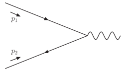
(a)

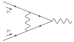
(b)

Figure 1: Tree and one loop diagrams contributing to the massive quark form factor in QED.

In this paper we consider the quark-antiquark annihilation process

$$q(p_{1})+\bar{q}(p_{2})\to\gamma^{*}(q),$$ (5)

whose tree and one loop contribution in QED is given respectively in Fig. 1 (a) and (b). Following Bernreuther:2004ih , the corresponding vertex function $V^{\mu}(p_{1},p_{2})$ is expressed in terms of two form factors, $F_{1}$ and $F_{2}$, as follows:

$$V^{\mu}(p_{1},p_{2}) = \bar{v}(p_{2})\,\Gamma^{\mu}(p_{1},p_{2})\,u(p_{1}),$$ (6)

$$\Gamma^{\mu}(p_{1},p_{2}) = -i\,e\,e_{q}\,\bigg{[}F_{1}\big{(}s,m^{2}\big{)}\gamma^{\mu}+\frac{1}{2m}F_{2}\big{(}s,m^{2}\big{)}\,i\,\sigma^{\mu\nu}q_{\nu}\bigg{]},$$ (7)

where $\sigma^{\mu\nu}=\frac{i}{2}[\gamma^{\mu},\gamma^{\nu}]$; furthermore, $s=(p_{1}+p_{2})^{2}$ represents the center of mass energy, and $m$ is the quark mass. The form factors $F_{i},\,i=1,2$ can be extracted by applying projection operators:

$$F_{i}\big{(}s,m^{2}\big{)}={\rm Tr}\big{[}P_{i}^{\mu}(m,p_{1},p_{2})\,\Gamma_{\mu}(p_{1},p_{2})\big{]},$$ (8)

where

$$P_{i}^{\mu}(m,p_{1},p_{2})=\frac{\not{p}_{1}+m}{m}\bigg{[}i\,g_{1}^{(i)}\gamma^{\mu}+\frac{i}{2m}g_{2}^{(i)}\big{(}p_{2}^{\mu}-p_{1}^{\mu}\big{)}\bigg{]}\frac{\not{p}_{2}-m}{m},$$ (9)

and

$$g_{1}^{(1)} = -\frac{1}{eN_{c}}\frac{1}{4(1-\epsilon)}\frac{1}{(s/m^{2}-4)},$$

$$g_{2}^{(1)} = \frac{1}{eN_{c}}\frac{3-2\epsilon}{(1-\epsilon)}\frac{1}{(s/m^{2}-4)^{2}},$$

$$g_{1}^{(2)} = \frac{1}{eN_{c}}\frac{1}{(1-\epsilon)}\frac{1}{s/m^{2}(s/m^{2}-4)},$$

$$g_{2}^{(2)} = -\frac{1}{eN_{c}}\frac{1}{(1-\epsilon)}\frac{1}{(s/m^{2}-4)^{2}}\bigg{[}\frac{4m^{2}}{s}+2-2\epsilon\bigg{]}.$$ (10)

In this paper we work in $d=4-2\epsilon$ dimensions, compute the unsubtracted form factor and omit counterterm insertions, which makes the mass $m$ the unrenormalized mass. The form factors have the perturbative expansion

$$F_{i}\left(s,m^{2},\mu^{2}\right) =F^{(0)}_{i}\left(s,m^{2}\right)+\frac{e_{q}^{2}\,\alpha_{\rm EM}}{4\pi}\,F^{(1)}_{i}\left(s,m^{2},\mu^{2}\right)$$

$$\hskip 85.35826pt+\bigg{(}\frac{e_{q}^{2}\,\alpha_{\rm EM}}{4\pi}\bigg{)}^{2}F^{(2)}_{i}\left(s,m^{2},\mu^{2}\right)+{\cal O}\left(\alpha_{\rm EM}^{3}\right)\,,$$ (11)

where

$$F^{(0)}_{1}\left(s,m^{2}\right)=1,\qquad\qquad\qquad F^{(0)}_{2}\left(s,m^{2}\right)=0.$$ (12)

We are interested in computing the higher order corrections in the small mass (or high-energy) limit $m^{2}/s\sim\lambda^{2}\ll 1$. We assume the center of mass frame, with the incoming quark moving along the positive $z$-axis. The momenta of the quark and anti-quark can then be decomposed along two light-like directions, $n_{\pm}=(1,0,0,\mp 1)$ as follows:

$$p^{\mu}_{1} = \left(\sqrt{p^{2}+m^{2}},0,0,p\right)=p_{1}^{+}\frac{n_{-}^{\mu}}{2}+p_{1}^{-}\frac{n_{+}^{\mu}}{2},$$

$$p^{\mu}_{2} = \left(\sqrt{p^{2}+m^{2}},0,0,-p\right)=p_{2}^{+}\frac{n_{-}^{\mu}}{2}+p_{2}^{-}\frac{n_{+}^{\mu}}{2}\,.$$ (13)

In the small mass limit the $p_{i}^{\pm}$ components have the scaling properties

$$p_{1}^{+} =n_{+}\cdot p_{1}=p_{2}^{-}=n_{-}\cdot p_{2}=\sqrt{p^{2}+m^{2}}+p\sim\sqrt{s},$$

$$p_{1}^{-} =n_{-}\cdot p_{1}=p_{2}^{+}=n_{+}\cdot p_{2}=\sqrt{p^{2}+m^{2}}-p\sim\lambda^{2}\sqrt{s}.$$ (14)

In what follows it will prove useful to define a variable

$$\hat{s}\equiv p_{1}^{+}p_{2}^{-}=\left(\sqrt{m^{2}+p^{2}}+p\right)^{2}\,,$$ (15)

such that

$$s=2m^{2}+p_{1}^{+}p_{2}^{-}+p_{1}^{-}p_{2}^{+}=2m^{2}+\hat{s}+\frac{m^{4}}{\hat{s}}.$$ (16)

We calculate the higher order corrections to the form factor in dimensional regularization, and use the method of expansion by regions Beneke:1997zp ; Smirnov:2002pj ; Jantzen:2011nz to evaluate the loop integrals in the limit $m^{2}\ll s$. In general one expects several regions to contribute. It is possible to use geometric methods (see e.g. Pak:2010pt ; Jantzen:2012mw ; Gardi:2022khw ) to reveal all regions contributing to an integral. In case of the problem at hand we find it is still possible to find all regions contributing up to two loops by straightforward inspection of the propagators in the loops. One advantage of this method is that the regions are directly associated to the scaling of the loop momenta, rather than to the scaling of Feynman parameters, as when geometric methods are used. This will allow us to relate more easily our results to the construction of an effective field theory description of the quark form factor, as effective field theories are typically constructed to reproduce the momentum regions of the present problem.

In what follows we decompose a generic momentum $k$ along the light-like directions $n_{\pm}$:

$$k^{\mu}=k^{+}\frac{n_{-}^{\mu}}{2}+k^{-}\frac{n_{+}^{\mu}}{2}+k_{\perp}^{\mu},\qquad\qquad\quad k^{\mu}=(k^{+},k^{-},k_{\perp}),$$ (17)

where $k_{\pm}=n_{\pm}\cdot k$. The second identity in the equation above provides a compact notation to indicate scaling relations. Up to one loop the following loop momentum modes contribute:

Hard ($$h k\sim\sqrt{\hat{s}}\,(\lambda^{0},\lambda^{0},\lambda^{0})\,,$$):

Collinear ($$c k\sim\sqrt{\hat{s}}\,(\lambda^{0},\lambda^{2},\lambda^{1})\,,$$): (18)

anti-Collinear ($$\bar{c} k\sim\sqrt{\hat{s}}\,(\lambda^{2},\lambda^{0},\lambda^{1})\,.$$):

As we will see in what follows, beyond one loop we find that two additional momentum modes are necessary, which scale as

Ultra-Collinear ($$uc k\sim\sqrt{\hat{s}}\,(\lambda^{2},\lambda^{4},\lambda^{3})\,,$$):

Ultra-anti-Collinear ($$\overline{uc} k\sim\sqrt{\hat{s}}\,(\lambda^{4},\lambda^{2},\lambda^{3})\,.$$): (19)

One might also expect the following modes to contribute:

Semi-Hard ($$sh k\sim\sqrt{\hat{s}}\,(\lambda^{1},\lambda^{1},\lambda^{1})\,,$$):

Soft ($$s k\sim\sqrt{\hat{s}}\,(\lambda^{2},\lambda^{2},\lambda^{2})\,,$$): (20)

however, these turn out to give rise to scaleless loop integrals and therefore do not contribute up to two-loop level.

Throughout the paper we define the loop integration measure in dimensional regularization as follows:

$$\int[dk]\equiv\bigg{(}\frac{\mu^{2}e^{\gamma_{E}}}{4\pi}\bigg{)}^{\epsilon}\int\frac{d^{4-2\epsilon}k}{(2\pi)^{4-2\epsilon}}.$$ (21)

In the limit $m^{2}\ll s$ we express the form factors as a power expansion in $m^{2}/\hat{s}$, and calculate the first two terms in the expansion. In general, the form factor is given as a sum over the contributing regions. At one loop we have for instance

$$F_{i}^{(1l)}\bigg{(}\frac{\mu^{2}}{\hat{s}},\frac{\mu^{2}}{m^{2}},\epsilon\bigg{)}=F_{i}^{(1l)}\Big{|}_{h}\bigg{(}\frac{\mu^{2}}{\hat{s}},\epsilon\bigg{)}+F_{i}^{(1l)}\Big{|}_{c}\bigg{(}\frac{\mu^{2}}{m^{2}},\epsilon\bigg{)}+F_{i}^{(1l)}\Big{|}_{\bar{c}}\bigg{(}\frac{\mu^{2}}{m^{2}},\epsilon\bigg{)}.$$ (22)

Each region is expected to depend non-analytically (logarithmically) on a single scale, which is dictated by the kinematics of the process. We find that the non-analytic dependence of the hard region is conveniently given in terms of the factor $\hat{s}$, while the non-analytic structure of the collinear and anti-collinear regions is given in terms of the mass $m$. At one loop only the single diagram of Fig. 1(b) contributes to the form factors and the region expansion is easy. The expansion of the corresponding scalar integral has been discussed at length in appendix A of Laenen:2020nrt , to which we refer for further details. Here we simply report the result, and postpone a more technical discussion concerning the region expansion for the two-loop calculation to Sec. 3. For the form factor $F_{1}$ we have

$$F_{1}^{(1l)}\Big{|}_{h} = \bigg{(}\frac{\mu^{2}}{-\hat{s}-i0^{+}}\bigg{)}^{\epsilon}\bigg{\{}-\frac{2}{\epsilon^{2}}-\frac{3}{\epsilon}-8+\zeta_{2}+\epsilon\bigg{(}-16+\frac{3\zeta_{2}}{2}+\frac{14\zeta_{3}}{3}\bigg{)}$$ (23)

$$\hskip 56.9055pt+\,\frac{m^{2}}{\hat{s}}\bigg{[}-\frac{2}{\epsilon}-6+\epsilon\big{(}-16+\zeta_{2}\big{)}\bigg{]}+{\cal O}(\epsilon^{2})+{\cal O}(\lambda^{4})\bigg{\}},$$

for the hard region, and

$$F_{1}^{(1l)}\Big{|}_{c} = \bigg{(}\frac{\mu^{2}}{m^{2}-i0^{+}}\bigg{)}^{\epsilon}\bigg{\{}\frac{1}{\epsilon^{2}}+\frac{2}{\epsilon}+4+\frac{\zeta_{2}}{2}+\epsilon\bigg{(}8+\zeta_{2}-\frac{\zeta_{3}}{3}\bigg{)}$$ (24)

$$\hskip 56.9055pt+\,\frac{m^{2}}{\hat{s}}\bigg{[}\frac{1}{\epsilon}+5+\epsilon\bigg{(}13+\frac{\zeta_{2}}{2}\bigg{)}\bigg{]}+{\cal O}(\epsilon^{2})+{\cal O}(\lambda^{4})\bigg{\}},$$

for the collinear region, and

$$F_{1}^{(1l)}\Big{|}_{\bar{c}}=F_{1}^{(1l)}\Big{|}_{c}.$$ (25)

In the prefactors in Eqs. (23) and (24), we have explicitly written the Feynman prescription $i0^{+}$, which upon expanding in $\epsilon$ give logarithms $\log(\mu^{2}/(-\hat{s}-i0^{+}))$ and $\log(\mu^{2}/(m^{2}-i0^{+}))$. For $\mu^{2}>0,m^{2}>0$ and $\hat{s}>0$ these can be rewritten using $\log(\mu^{2}/(-\hat{s}-i0^{+}))\rightarrow\log(\mu^{2}/\hat{s})+i\pi$ and $\log(\mu^{2}/(m^{2}-i0^{+}))\rightarrow\log(\mu^{2}/m^{2})$ to obtain the imaginary parts. For notational convenience, we will drop the Feynman prescription in what follows and note that these can always be reinstated by $\hat{s}\rightarrow\hat{s}+i0^{+}$ and $m^{2}\rightarrow m^{2}-i0^{+}$ after which the imaginary parts can be retrieved adopting the rule described above.

The form factor $F_{2}$ starts at NLP. We have

$$F_{2}^{(1l)}\Big{|}_{h} = \bigg{(}\frac{\mu^{2}}{-\hat{s}}\bigg{)}^{\epsilon}\bigg{\{}\frac{m^{2}}{\hat{s}}\bigg{[}\frac{4}{\epsilon}+16+\epsilon\big{(}32-2\zeta_{2}\big{)}\bigg{]}+{\cal O}(\epsilon^{2})+{\cal O}(\lambda^{4})\bigg{\}},$$ (26)

and

$$F_{2}^{(1l)}\Big{|}_{c} = \bigg{(}\frac{\mu^{2}}{m^{2}}\bigg{)}^{\epsilon}\bigg{\{}\frac{m^{2}}{\hat{s}}\bigg{[}-\frac{2}{\epsilon}-8+\epsilon\big{(}-16-\zeta_{2}\big{)}\bigg{]}+{\cal O}(\epsilon^{2})+{\cal O}(\lambda^{4})\bigg{\}},$$ (27)

and

$$F_{2}^{(1l)}\Big{|}_{\bar{c}}=F_{2}^{(1l)}\Big{|}_{c}.$$ (28)

These results can be compared directly with Bernreuther:2004ih by extracting the coefficients ${\cal F}^{(1)}_{i}(s,\mu)$ as defined in Eq. (18) there, as follows

$${\cal F}^{(1)}_{i}(s,\mu)=\frac{e^{-\epsilon\gamma_{E}}}{\Gamma(1+\epsilon)}\bigg{(}\frac{\mu^{2}}{m^{2}}\bigg{)}^{-\epsilon}F^{(1)}_{i}(s,\mu).$$ (29)

Summing over the regions and expanding also the scale factors in powers of $\epsilon$ we find

$${\cal F}^{(1)}_{1}(s,\mu) = \bigg{\{}\frac{1}{\epsilon}\bigg{[}1-2\ln\bigg{(}-\frac{m^{2}}{\hat{s}}\bigg{)}\bigg{]}-3\ln\bigg{(}-\frac{m^{2}}{\hat{s}}\bigg{)}-\ln^{2}\bigg{(}-\frac{m^{2}}{\hat{s}}\bigg{)}+2\zeta_{2}$$ (30)

$$\hskip 28.45274pt+\,\frac{m^{2}}{\hat{s}}\bigg{[}4-2\ln\bigg{(}-\frac{m^{2}}{\hat{s}}\bigg{)}\bigg{]}+{\cal O}(\epsilon)+{\cal O}(\lambda^{4})\bigg{\}},$$

and

$${\cal F}^{(1)}_{2}(s,\mu) = 4\frac{m^{2}}{\hat{s}}\ln\bigg{(}-\frac{m^{2}}{\hat{s}}\bigg{)}+{\cal O}(\epsilon)+{\cal O}(\lambda^{4}),$$

in agreement with the high-energy expansion $s\gg m^{2}$ of eqs. (19) and (20) of Bernreuther:2004ih .

The massive form factor at two-loop was first computed in QED in Bonciani:2003ai , followed by Bernreuther:2004ih , which considered its generalization to QCD. The former provides the full result at the level of the individual diagrams, while the latter presents results with all diagrams combined, see Eqs. (22) and (23) in Bernreuther:2004ih for $F_{1}$ and $F_{2}$ respectively for more details.

3 Calculational steps

Here we describe the general approach that we adopt throughout the rest of this work, deferring a discussion of technical details to Sec. 4. In Sec. 3.1, we present the diagrams that contribute to the two-loop massive form factor, followed by a discussion of their associated integrals and their classification into three different topologies denoted by $A$, $B$ and $X$ in Sec. 3.2. We conclude the section with a brief summary in Sec. 3.3 where we preview various subtleties that we shall encounter in Sec. 4.

3.1 Diagrams contributing to the two-loop form factor

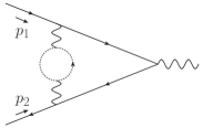
(a)

(b)

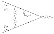
(c)

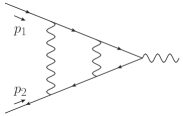
(d)

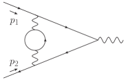
(e)

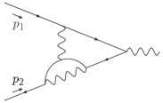
(f)

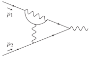
(g)

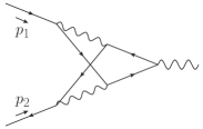
(h)

Figure 2: Diagrams that contribute to the massive form factor at two-loop in QED. Dashed lines represent massless fermions.

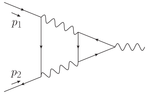
Figure 3: Diagrams with a closed fermion loop that cancel in QED by Furry’s theorem PhysRev.51.125 .

The diagrams that contribute to the massive form factor at two-loop are displayed in Fig. 2. There are eight diagrams in total, labeled (a) - (h), with $p_{1}$ and $p_{2}$ denoting the external momenta of the two incoming fermions. Solid and dashed lines are used to represent massive and massless fermions respectively. Fig. 3 suggests there are two additional diagrams to account for, but these diagrams cancel by Furry’s theorem PhysRev.51.125 . Concerning diagram (e), note that the fermion running inside the loop does not need to correspond to those on the external lines, but here we ignore this possibility for simplicity as it would introduce an additional hierarchy of scales that makes the power counting much more involved. Diagrams (b) and (c), as well as (f) and (g), are related by exchanging $p_{1}$ and $p_{2}$ and therefore we expect this symmetry to be present also during an expansion by regions.

In anticipation of our regional analysis, it is convenient to classify diagrams (a) to (h) into three different topologies labeled $A$, $B$ and $X$ which are distinguished by the flow of their internal momenta.

3.2 Topology classification

Starting with diagrams (a)-(d), we note that the Feynman integrals contributing to these diagrams share the following parameterization

$$I_{A;\{n_{i}\}} \equiv\int[dk_{1}][dk_{2}]\frac{1}{k_{1}^{2n_{1}}}\frac{1}{k_{2}^{2n_{2}}}\frac{1}{[(k_{1}-k_{2})^{2}]^{n_{3}}}\frac{1}{[(k_{1}+p_{1})^{2}-m^{2}]^{n_{4}}}\frac{1}{[(k_{2}+p_{1})^{2}-m^{2}]^{n_{5}}}$$

$$\hskip 142.26378pt\times\frac{1}{[(k_{1}-p_{2})^{2}-m^{2}]^{n_{6}}}\frac{1}{[(k_{2}-p_{2})^{2}-m^{2}]^{n_{7}}}\,,$$ (31)

which we define as topology $A$. In Eq. (31), $k_{1}$ and $k_{2}$ denote the internal loop momenta and the integer $n_{i}$ represents the generic power associated to the $i$th propagator.

In a similar way, the integrals associated to diagrams (e), (f) and (g) in Fig. 2 can be parameterized by

$$I_{B;\{n_{i}\}}^{b_{3},b_{4},b_{5},b_{6}} \equiv\int[dk_{1}][dk_{2}]\frac{1}{[k_{1}^{2}-m^{2}]^{n_{1}}}\frac{1}{[k_{2}^{2}-m^{2}]^{n_{2}}}\frac{\mu_{3}^{2b_{3}}}{[(k_{1}-p_{1})^{2}]^{n_{3}+b_{3}}}$$ (32)

$$\times\frac{\mu_{4}^{2b_{4}}}{[(k_{1}+k_{2}-p_{1})-m^{2}]^{n_{4}+b_{4}}}\frac{\mu_{5}^{2b_{5}}}{[(k_{1}+p_{2})^{2}]^{n_{5}+b_{5}}}\frac{\mu_{6}^{2b_{6}}}{[(k_{1}+k_{2}+p_{2})-m^{2}]^{n_{6}+b_{6}}}\frac{1}{[(k_{1}+k_{2})^{2}]^{n_{7}}}\,,$$

and this defines topology $B$. An important distinction compared to topology $A$ is the appearance of the complex numbers $b_{i}$ associated to propagators $3,4,5$ and 6, where artificial scales $\mu_{i}$ with unit mass dimensions have been introduced on dimensional grounds. The need for the powers $b_{i}$ can be seen as follows. When expanding in momentum regions, one finds eikonal propagators that contain only the $k_{i}^{+}$ or $k_{i}^{-}$ momentum components. As a result, additional divergences may arise from the $k_{i}^{+}$ and $k_{i}^{-}$ integrals because the dimensional parameter $\epsilon$ regulates only the transverse momentum components $k_{i,\perp}$. Various regulators have been introduced in the literature to tame these rapidity divergences, e.g. space-like Wilson-lines collins_2023 , $\delta$ regulators Echevarria:2011epo ; Echevarria:2012js ; Echevarria:2015usa ; Echevarria:2015byo ; Echevarria:2016scs , $\eta$ regulators Chiu:2011qc ; Chiu:2012ir , exponential regulators Li:2016axz , analytic regulators Beneke:2003pa ; chiu:2007yn ; Becher:2010tm ; Becher:2011dz and pure rapidity regulators Ebert:2018gsn . In this work, we adopt the analytic regulator Beneke:2003pa , meaning that we raise the relevant propagators to complex powers $b_{i}$. The rapidity divergences then manifest themselves as poles in $b_{i}$, similar to poles in $\epsilon$ that one encounters in dimensional regularization. As will be described in greater detail in Sec. 4.2, one does not need to add all four regulators $b_{i}$ simultaneously to regulate the rapidity divergences present in diagrams (e), (f) and (g). However, we do need to make different choices per diagram, and therefore the parameterization in Eq. (32) captures all three diagrams at once. Furthermore, we point out that the $b_{i}$’s do not need to be different; in fact, we will see that only a single regulator is sufficient in topology $B$. We refer to App. A for more details, as well as for a study on the use of other rapidity regulators. Note that the rapidity divergences show up only as a result of the expansion by regions, since the corresponding full Feynman integral gets fully regularized by the dimensional regulator $\epsilon$ alone. This observation provides us with a valuable cross-check: all dependence on $b_{i}$ must cancel once all regions are combined.

Finally, we come to topology $X$, which corresponds to diagram (h) and is characterized by the parameterization

$$I_{X;\{n_{i}\}}^{b_{3},b_{4},b_{5},b_{6}} =\int[dk_{1}][dk_{2}]\frac{1}{k_{1}^{2n_{1}}}\frac{1}{k_{2}^{2n_{2}}}\frac{\mu_{3}^{2b_{3}}}{[(k_{2}-p_{1})^{2}-m^{2}]^{n_{3}+b_{3}}}\frac{\mu_{4}^{2b_{4}}}{[(k_{1}+k_{2}-p_{1})^{2}-m^{2}]^{n_{4}+b_{4}}}$$

$$\hskip 28.45274pt\times\frac{\mu_{5}^{2b_{5}}}{[(k_{1}+p_{2})-m^{2}]^{n_{5}+b_{5}}}\frac{\mu_{6}^{2b_{6}}}{[(k_{1}+k_{2}+p_{2})^{2}-m^{2}]^{n_{6}+b_{6}}}\frac{1}{[(k_{1}+k_{2})^{2}]^{n_{7}}}\,,$$ (33)

where again we need $b_{i}\neq 0$ in order to regulate rapidity divergences that show up once we expand by region.

3.3 Summary of technical details

A common approach in the computation of higher order loop diagrams is to reduce the many Feynman integrals to master integrals using integration by parts (IBP) identities. When it comes to calculating these integrals following the method of regions one has two alternative options. Either one first reduces the large number of integrals in each topology, Eqs. (31)-(33), to master integrals before expanding by regions. However, as we are interested in an expansion up to NLP, the expansion of a master integral into its momentum regions might lead to many additional integrals, so that again a new reduction to master integrals is recommended per momentum region. Therefore, one might as well first expand by regions and only perform an IBP reduction at the very end of the calculational steps. Ultimately, these two ways are equivalent and cannot lead to different final results. We will discuss these alternative approaches further in Sec. 4.1, where we also point out the subtleties that enter while expanding the topologies in different momentum regions.

Another difficulty we encountered concerns the analytic regulators that we added to topologies $B$ and $X$, Eqs. (32) and (33). Although the analytic regulator is a convenient regulator when computing Feynman integrals, it has the downside that the usual IBP reduction programs cannot handle non-integer powers of the propagators. To the best of our knowledge, only Kira Klappert:2020nbg is suitable for this, which we therefore adopt as our standard IBP reduction program. In topology $A$, which does not require rapidity regulators, we also use LiteRed Lee:2013mka as an independent crosscheck of our results.

As discussed in Sec. 2, the one-loop form factor contains just three momentum regions: hard, collinear and anti-collinear. However, the number of momentum regions is much larger at the two-loop level. First, the two loop momenta $k_{1}$ and $k_{2}$ can have different scalings, which gives already nine possibilities that combine the hard, collinear and anti-collinear momentum regions. Second, we find the appearance of two new momenta scalings: ultra-collinear and ultra-anti-collinear; the contribution from such regions was already observed in Smirnov:1999bza . Finally for topology $B$ and X, new regions might appear when one shifts the loop momenta before expanding in regions. Although such a shift leaves the full integral invariant, it can lead to additional regions when expanding.

A summary of our work flow is given in Fig. 4, which shows the steps we have discussed so far. Not shown is the final step, which consists of verifying whether the small mass limit as given in Bonciani:2003ai ; Bernreuther:2004ih is reproduced after collecting all regions.

Figure 4: Flow diagram displaying the pipeline of our NLP region analysis of the QED massive form factor. The diagrams in Fig. 2 are classified into either topology $A$, $B$ or $X$ depending on their momentum flow. We regulate each topology using dimensional regularization, denoted by $\epsilon$, plus additional rapidity regulators, denoted $\nu$, in case of topology $B$, and $\nu_{1},\nu_{2}$ in case of topology $X$, as it turns out to need two rapidity regulators. For each topology, we expand the relevant integrals by regions and then reduce the result into a simpler set of master integrals with IBP reduction using Kira Klappert:2020nbg .

4 Region expansions

Having presented the computational scheme in Sec. 3, we now move to the technical details of the calculation of the integrals in topology $A$, $B$ and $X$ using the method of regions. An important remark from the outset concerns the distinction between the regions present at the level of the diagrams in Fig. 2 on the one hand, and the integral level on the other hand; these do not necessarily coincide as non-vanishing regions at the integral level can cancel when combined to constitute the diagrams. The results presented in this section should be understood at the integral level.

We shall now discuss topology $A$, $B$ and $X$ in turn. For each topology, we analyze first the associated regions (at the integral level), followed by a discussion of its IBP relations. At the end of each topology subsection, we provide a brief summary of the aspects that enter its computation.

4.1 Region expansion of topology $A$

As explained in Sec. 2, it is convenient to use light-cone coordinates, Eq. (17), to identify the various momentum regions that lead to non-vanishing contributions. At one-loop we found that only momentum modes $h$, $c$ and $\bar{c}$ contributed. This picture changes as soon as we move to the two-loop level where we receive additional contributions coming from momentum modes such as $uc$ and $\overline{uc}$, as defined in Eq. (19). In total, there are 25 possible combinations of momentum modes at the two-loop level. However, many combinations vanish because they lead to scaleless integrals. For the Feynman integrals contributing to diagrams (a)-(d) we find 11 non-vanishing regions: $hh$, $cc$, $\bar{c}\bar{c}$, $c\bar{c}$, $\bar{c}c$, $ch$, $hc$, $\bar{c}h$, $h\bar{c}$, $uc\bar{c}$ and $\overline{uc}c$, with the momentum flow as indicated in Tab. 2 on page 2.

	$k^{2}$	$k^{+}p_{1}^{-}$	$k^{-}p_{1}^{+}$	$k^{+}p_{2}^{-}$	$k^{-}p_{2}^{+}$
$(h)$	1	$\lambda^{2}$	1	1	$\lambda^{2}$
$(c)$	$\lambda^{2}$	$\lambda^{2}$	$\lambda^{2}$	1	$\lambda^{4}$
($\bar{c}$)	$\lambda^{2}$	$\lambda^{4}$	1	$\lambda^{2}$	$\lambda^{2}$
$(uc)$	$\lambda^{6}$	$\lambda^{4}$	$\lambda^{4}$	$\lambda^{2}$	$\lambda^{6}$
($\overline{uc}$)	$\lambda^{6}$	$\lambda^{6}$	$\lambda^{2}$	$\lambda^{4}$	$\lambda^{4}$

Table 1: Scaling associated to the different momentum regions.

Even though the power expansion for the momentum modes is straightforward using e.g. Tab. 1, the resulting integrals can in general become quite involved. Let us illustrate this by highlighting several subtleties that enter here.

The first subtlety we want to discuss concerns the interplay between the usual IBP reduction and the region expansion. To this end, we consider as an example the $hh$ region of topology $A$, Eq. (31), which up to LP reads

$$I_{A}\Big{|}_{hh} =\int[dk_{1}][dk_{2}]\frac{1}{k_{1}^{2n_{1}}}\frac{1}{k_{2}^{2n_{2}}}\frac{1}{[(k_{1}-k_{2})^{2}]^{n_{3}}}\frac{1}{[k_{1}^{2}+k_{1}^{-}p_{1}^{+}]^{n_{4}}}\frac{1}{[k_{2}^{2}+k_{2}^{-}p_{1}^{+}]^{n_{5}}}$$

$$\hskip 142.26378pt\frac{1}{[k_{1}^{2}-k_{1}^{+}p_{2}^{-}]^{n_{6}}}\frac{1}{[k_{2}^{2}-k_{2}^{+}p_{2}^{-}]^{n_{7}}}+\mathcal{O}\left(\lambda^{2}\right)\,,$$ (34)

while many additional terms occur beyond LP. To see this, we expand the fourth propagator of Eq. (31) in the $hh$-region up to NLP

$$\frac{1}{(k_{1}+p_{1})-m^{2}} =\frac{1}{k_{1}^{2}+k_{1}^{-}p_{1}^{+}}-\frac{k_{1}^{+}p_{1}^{-}}{[k_{1}^{2}+k_{1}^{-}p_{1}^{+}]^{2}}+\mathcal{O}\left(\lambda^{4}\right)$$

$$=\frac{1}{k_{1}^{2}+k_{1}^{-}p_{1}^{+}}-\frac{m^{2}}{\hat{s}}\frac{k_{1}^{2}-[k_{1}^{2}-k_{1}^{+}p_{2}^{-}]}{[k_{1}^{2}+k_{1}^{-}p_{1}^{+}]^{2}}+\mathcal{O}\left(\lambda^{4}\right)\,.$$ (35)

On the last line of Eq. (35) we used the identity $p_{1}^{-}=\left(m^{2}/\hat{s}\right)p_{2}^{-}$ to rewrite the power expansion in terms of the first, fourth and sixth LP (inverse) propagators appearing in Eq. (34). Typically, one can perform an IBP reduction on the full integrals for a given diagram and then expand by regions. However, Eq. (35) shows that after the regions expansion, the number of integrals increases considerably again beyond LP. Therefore, a new IBP reduction applied to the $hh$-region is called for. Instead, one might just as well expand the full integrals in the momentum region, and perform a single IBP-reduction on region integrals at the end.

As a second subtlety, note that, in order to set up the IBP reduction for the expanded topology, the LP propagators of Eq. (34) appear in the last line of Eq. (35). Similarly, as shown for the fourth propagator in Eq. (35), we can rewrite the power expansion of the fifth, sixth and seventh propagator in terms of the corresponding LP propagators, where we can use the identity $p_{2}^{+}=\left(m^{2}/\hat{s}\right)p_{1}^{+}$ for the sixth and seventh propagator. This implies that Eq. (34) defines a closed topology for the $hh$-region up to arbitrary order in the power expansion. This is particularly useful when applying IBP relations, because it leads to the least number of master integrals to solve. Along similar lines, the full power expansion of the $cc$ and $\bar{c}\bar{c}$ region can also be written in terms LP propagators only.

Another subtlety concerns regions where the loop momenta $k_{1}$ and $k_{2}$ scale according to different momentum modes, which requires extending the expanded topology by an additional propagator. For example, consider the expansion of the denominator of the third propagator in Eq. (31) in the $\bar{c}c$ region

$$(k_{1}-k_{2})^{2}=\underbrace{k_{1}^{2}-2k_{1,\perp}\cdot k_{2,\perp}+k_{2}^{2}}_{\sim\lambda^{2}}-\underbrace{k_{1}^{-}k_{2}^{+}}_{\sim 1}-\underbrace{k_{1}^{+}k_{2}^{-}}_{\sim\lambda^{4}}\,.$$ (36)

The perpendicular components in Eq. (36) cannot be rewritten in terms of the LP propagators from Eq. (31). Rather than adding $-2k_{1,\perp}\cdot k_{2,\perp}$ to the $\bar{c}c$ topology, we instead rewrite this as

$$-2k_{1,\perp}\cdot k_{2,\perp}=-2k_{1}\cdot k_{2}+k_{1}^{+}k_{2}^{-}+k_{1}^{-}k_{2}^{+}\,,$$ (37)

and add $[-2k_{1}\cdot k_{2}]^{-n_{8}}$ as an additional propagator to the $\bar{c}c$ topology. The same logic can be applied to other regions where $k_{1}$ and $k_{2}$ scale differently. Eq. (37) shows that standard propagators may turn into non-standard propagators of the form $k_{1}^{-}k_{2}^{+}$ which cannot be given as input to the current IBP programs directly. We treat these in the following way, which we will refer to as a loop-by-loop approach. First, we rewrite $k_{1}^{-}k_{2}^{+}$ as $k_{1}\cdot(k_{2}^{+}n^{-})$ and perform an IBP reduction over $k_{1}$ while considering $k_{2}$ and $k_{2}^{+}n^{-}$ as external momenta similar to $p_{1}$ and $p_{2}$. By doing so, the integrals over $k_{1}$ get reduced to a smaller set of integrals. Next, we repeat the first step but now switching the roles of $k_{2}$ and $k_{1}$, i.e. we perform IBP over $k_{2}$ rewriting $k_{1}^{-}k_{2}^{+}$ as $(k_{1}^{-}n^{+})\cdot k_{2}$, while considering $k_{1}$ and $k_{1}^{-}n^{+}$ as external momentum. Again, the number of integrals over $k_{2}$ gets reduced. The combination of both IBP reductions over $k_{1}$ and $k_{2}$ leaves us with a smaller set of (two-loop) integrals to solve.

Finally, one must be careful when dealing with regions where one of the loop momenta has hard scaling and the other has (anti-)collinear scaling. As discussed above, one can define a closed topology containing the LP propagators and the addition of an eighth propagator $[-2k_{1}\cdot k_{2}]^{-n_{8}}$. However, because a loop-by-loop IBP reduction may lead to new propagators that are not part of the (expanded) topology, adding these propagators to the topology does not work as this leads to an over-determined topology. A possible solution, which we used for topology $A$, is to perform the IBP reduction over the loop with hard loop momentum and then compute the masters. After that, the left-over one-loop integrals with (anti-)collinear loop momentum will be simple enough to calculate directly.

Let us summarize our strategy for topology $A$:

1. Expand Eq. (31) in a given momentum region and rewrite subleading corrections in terms of the LP propagators.

2. Use IBP relations that can either handle both loops over $k_{1}$ and $k_{2}$ at the same time or adopt a loop-by-loop approach by introducing a non-standard additional propagator $[-2k_{1}\cdot k_{2}]^{-n_{8}}$.

3. Solve the resulting master integrals and repeat steps 1-3 for the remaining momentum regions.

4.2 Region expansion of topology $B$

As we already stated in Sec. 3, the Feynman integrals needed to calculate diagrams (e), (f) and (g) in Fig. 2 can be classified as part of topology $B$, defined in Eq. (32). More specifically, all integrals obtained from diagram (e) have the form $I_{B;\{n_{i}\}}^{b_{3},b_{4},b_{5},b_{6}}$ with both $n_{3}\leq 0$ and $n_{5}\leq 0$, the integrals of diagrams (f) satisfy $n_{3}\leq 0$, while the integrals of diagrams (g) correspond to $n_{5}\leq 0$. The integrals of diagrams (e) thus belong to a subclass of the integrals associated to diagrams (f) and (g). Consequently, the regions contributing to diagram (e) form a subset of those contributing to diagram (f) and (g). In addition, the integrals of diagram (f) and diagram (g) can be related to each other by the transformation $p_{1}\leftrightarrow p_{2}$, $k_{1}\leftrightarrow-k_{1}$ and $k_{2}\leftrightarrow-k_{2}$. In the following we will discuss the regions obtained in diagrams (e), (f) and (g).

Diagram (e)

Starting with the integrals of diagram (e), we find that the regions $hh$, $hc$, $\bar{c}h$, $cc$ and $\bar{c}\bar{c}$ contribute. Of these, the first three regions are free of rapidity divergences, so that we can set the analytic regulators $b_{i}=0$ in Eq. (32) either at the beginning or at the end of the calculation (both leading to the same results). Taking $b_{i}=0$ from the start, we can treat these three regions similar to the corresponding regions in topology $A$, as we discussed in Sec. 4.1. However, there are two other regions, the $cc$ and $\bar{c}\bar{c}$ regions, that do have rapidity divergences, so that here the regulators $b_{i}$ must be kept. However, we do not need to include four regulators $b_{i}$ in the calculation. Because $n_{3}\leq 0$ and $n_{5}\leq 0$ we can safely take $b_{3}=0$ and $b_{5}=0$ at the beginning of the calculation. Interestingly, we find that we cannot take $b_{4}=b_{6}$ to regulate the rapidity divergences of all integrals, although taking either $b_{4}=0$ or $b_{6}=0$ is possible. We therefore choose $b_{6}=\nu$ and $b_{3}=b_{4}=b_{5}=0$ with corresponding scale $\mu_{6}=\tilde{\mu}$ as our scheme to regulate the rapidity divergences in both the $cc$ and $\bar{c}\bar{c}$ regions of diagram (e). Note that this particular choice breaks the symmetry between the $cc$ and $\bar{c}\bar{c}$ regions. Nevertheless, after combining all of the above five regions, our result up to NLP for each integral, has noy rapidity divergence. Moreover we find agreement with the corresponding result obtained by expanding the full result in Ref. Bonciani:2003te ; Gluza:2009yy in the small mass limit.

Diagram (f)

The regions needed to calculate the integrals of diagram (f) are more complicated. First, the integrals of diagram (f) satisfy $n_{3}\leq 0$. Similar to diagram (e), we encounter rapidity divergences in the $cc$ and $\bar{c}\bar{c}$ regions, and in order to handle those we take $b_{3}=b_{4}=0$ and $b_{5}=b_{6}=\nu$ with corresponding scale $\mu_{5}=\mu_{6}=\tilde{\mu}$. However, we find that the rapidity divergences do not cancel after summing the $cc$ and $\bar{c}\bar{c}$ regions. We therefore expect that there is at least one more region with rapidity divergences.

Indeed, in addition to the five regions for diagram (e) ($hh$, $hc$, $\bar{c}h$, $cc$ and $\bar{c}\bar{c}$), we find three additional contributing regions, although it is not straightforward to define these three regions in momentum space using the definition for $I_{B;\{n_{i}\}}^{b_{3},b_{4},b_{5},b_{6}}$ in Eq. (32). We exploit the freedom to shift $k_{2}\rightarrow-k_{1}-k_{2}$ to redefine topology $B$ as

$${I^{\prime}\,}_{B;\{n_{i}\}}^{b_{3},b_{4},b_{5},b_{6}} =\int[dk_{1}][dk_{2}]\frac{1}{[k_{1}^{2}-m^{2}]^{n_{1}}}\frac{1}{[(k_{1}+k_{2})^{2}-m^{2}]^{n_{2}}}\frac{\mu_{3}^{2b_{3}}}{[(k_{1}-p_{1})^{2}]^{n_{3}+b_{3}}}$$ (38)

$$\hskip 14.22636pt\times\frac{\mu_{4}^{2b_{4}}}{[(k_{2}+p_{1})^{2}-m^{2}]^{n_{4}+b_{4}}}\frac{\mu_{5}^{2b_{5}}}{[(k_{1}+p_{2})^{2}]^{n_{5}+b_{5}}}\frac{\mu_{6}^{2b_{6}}}{[(k_{2}-p_{2})^{2}-m^{2}]^{n_{6}+b_{6}}}\frac{1}{k_{2}^{2n_{7}}}\,.$$

We stress that $I_{B;\{n_{i}\}}^{b_{3},b_{4},b_{5},b_{6}}$ and ${I^{\prime}\,}_{B;\{n_{i}\}}^{b_{3},b_{4},b_{5},b_{6}}$ are equivalent before region expansion due to the Lorentz invariance, but this is not always the case for a given region, i.e. after expansion. For example, in the $cc$-region, the loop momenta $k_{1}$ and $k_{2}$ have the same momentum mode and as a result, the shift $k_{2}\rightarrow-k_{1}-k_{2}$ does not change the scale of the propagators nor the results of the integrals. However, in the $hc$-region, the shift $k_{2}\rightarrow-k_{1}-k_{2}$ changes the leading behavior of the second, fourth, sixth and seventh propagator of $I_{B;\{n_{i}\}}^{b_{3},b_{4},b_{5},b_{6}}$ and as a result we find a different $hc$-region through this shift. In general, one must be aware that different momentum flows can lead to a different scaling of the leading term in the propagator and uncover additional regions as a result. This illustrates the alternative viewpoint that regions correspond to the scaling of the leading term in the propagators rather than the loop momenta itself, a reasoning which connects also to the geometric approach in parameter space. However, in view of factorization, it is more convenient to still think about the scaling of the momentum modes of the loop momenta, rather than the scaling of the leading term in the propagators.

Based on the new definition ${I^{\prime}\,}_{B;\{n_{i}\}}^{b_{3},b_{4},b_{5},b_{6}}$, we find three additional regions: $\bar{c}c^{\prime}$, $hc^{\prime}$ and $\bar{c}uc^{\prime}$, as illustrated in Fig. 5.

Figure 5: Momentum regions that contribute to the integrals of diagram (f) before and after applying the transformation $k_{2}\rightarrow-k_{1}-k_{2}$, corresponding to $I_{f}$ and $I_{f}^{\prime}$ respectively. The dashed arrows represent how the regions in $I_{f}$ transform accordingly, e.g. the original $hc$-region maps onto a new $hh$-region after the collinear mode $k_{2}$ mixes with the dominant hard scale associated to $k_{1}$. Note how two previously uncovered regions, $\bar{c}c^{\prime}$ and $\bar{c}uc^{\prime}$, and a different $hc$-region appear after the shift, where the $\bar{c}c^{\prime}$-region removes the rapidity divergences present in the $cc$ and $\bar{c}\bar{c}$ regions. Regions that remain invariant are displayed on top of each other, while additional regions are shifted outwards such that all regions are found by collapsing the top row onto its base $I_{f}$.

Besides a modified $hc$-region, we also find $\bar{c}c^{\prime}$ and $\bar{c}uc^{\prime}$ as complete new regions. Apart from these three regions, we do not need other regions based on ${I^{\prime}\,}_{B;\{n_{i}\}}^{b_{3},b_{4},b_{5},b_{6}}$, as these are the same as the corresponding regions given based on ${I}_{B;\{n_{i}\}}^{b_{3},b_{4},b_{5},b_{6}}$. The appearance of the $\bar{c}uc^{\prime}$-region for example can be understood as follows (the $\bar{c}c^{\prime}$-region following similarly). First, note that the last propagator, $1/k_{2}^{2}$, in Eq. (38) has ultra-collinear scaling in the $\bar{c}uc^{\prime}$-region. Having found this region in this way, it is also clear that we could not have found it in the original momentum routing. First, it is not possible to select scalings of both loop momenta such that the last momentum factor is ultra-collinear. Second, it is only possible to make the last propagator have an ultra-collinear scaling unless one considers the $ucuc$-region, which leads to scaleless integrals. This is because the masses and external momenta in the propagators of Eq. (32) have harder scales than the loop momentum with an ultra-(anti-)collinear mode, thus kinematic configurations where one of the loop momenta is ultra-(anti-)collinear are always scaleless. In other words, in the parametrization of Eq. (32), the propagator $(k_{1}+k_{2})^{2}$ can produce a leading term with $uc$ scaling only if $k_{1}$ and $k_{2}$ are large and opposite, such as to almost cancel. Thus this ultra-collinear kinematic configuration can only be revealed by the shift leading to the parametrization in Eq. (38). A similar circumstance has been discussed in Ref. Bahjat-Abbas:2018hpv at one-loop, where a soft region arises in the kinematic configuration in which the loop momentum is large and opposite to an external momentum, such that their sum is soft. In general, revealing such regions by means of momentum shifts in order to find the scaling of the leading term may become ever more intricate at higher loops, due to an increasing number of loop momenta that can conspire to yield new regions. We can still validate our results in another way though. Combining the new $\bar{c}c^{\prime}$-region with the $cc$-region and $\bar{c}\bar{c}$-region from before the shift, we remove all the rapidity divergences belonging to the integrals of diagram (f). Furthermore, combining all of the above eight regions, we obtain the result up to NLP for each integral of diagram (f), reproducing the corresponding result found by expanding the exact result in Refs. Bonciani:2003te ; Gluza:2009yy in the small mass limit.

Diagram (g)

All the Feynman integrals for diagram (g) fall in the category of Eq. (32) with $n_{5}\leq 0$. Diagram (g) is related to diagram (f) by the transformation $p_{1}\leftrightarrow p_{2}$, $k_{1}\leftrightarrow-k_{1}$ and $k_{2}\leftrightarrow-k_{2}$. Naturally the rapidity regulators should also be exchanged: $b_{3}\leftrightarrow b_{5}$ and $b_{4}\leftrightarrow b_{6}$. Thus we choose as rapidity regulators $b_{3}=b_{4}=\nu$ and $b_{5}=b_{6}=0$ with corresponding scales $\mu_{3}=\mu_{4}=\tilde{\mu}$. All the regions from diagram (f), corresponding to the $hh$, $h\bar{c}$, $ch$, $cc$ and $\bar{c}\bar{c}$, $c\bar{c}^{\prime}$, $h\bar{c}^{\prime}$ and $c\overline{uc}^{\prime}$ regions can then be copied.

Remarks

Above we discussed how one can apply the rapidity regulators and find all the contributing regions per diagram. However, the calculation of the integrals in each region is not always straightforward and we therefore finish the discussion of topology $B$ with a few technical remarks on these calculations.

First, regarding regions without rapidity divergences, such as the $hh$, $hc$ and $c\overline{uc}^{\prime}$ regions, we can safely set $\nu=0$ and calculate the resulting integrals in each region following the same methods as for topology $A$. We emphasize however that in topology $B$ (and also in topology $X$ below) for the region including a hard loop momentum and a (anti-)collinear momentum, one should be quite careful when calculating the expanded integrals. Specifically, one should first expand the full integral $I_{B;\{n_{i}\}}^{b_{3},b_{4},b_{5},b_{6}}$ into regions, e.g. the $hc$-region, and only then perform IBP reduction on the part with hard loop momentum. Then $I_{B;\{n_{i}\}}^{b_{3},b_{4},b_{5},b_{6}}$ will be expressed as a linear combination of one-loop integrals, which we generically denote by $I^{c}_{i}$, which include only the collinear-mode loop momentum. Although in the $hc$-region $I_{B;\{n_{i}\}}^{b_{3},b_{4},b_{5},b_{6}}$ is free of rapidity divergences and the $b_{i}$ have been set to zero, we find that rapidity divergences reappear in some of these $I^{c}_{i}$. The rapidity divergences are however expected to cancel among different $I^{c}_{i}$ leading to a finite $I_{B;\{n_{i}\}}^{b_{3},b_{4},b_{5},b_{6}}$. In this particular case, one should choose an auxiliary regulator to regulate $I^{c}_{i}$. The poles in this auxiliary regulator will then cancel to yet yield a finite $I_{B;\{n_{i}\}}^{b_{3},b_{4},b_{5},b_{6}}$. Alternatively one can rearrange the integrands of $I^{c}_{i}$ at the level of Feynman parametrization such that the integrations over the Feynman parameters are well-defined and finite without introducing extra regulators.

We use the first method to calculate the integrals in the region including a hard loop momentum and a (anti-)collinear momentum, which is more convenient than the second one when dealing with a large number of such integrals. We also use the second method to calculate several integrals, always leading to the same results. Note that such complexity does not appear in topology $A$.

Then, for regions with rapidity divergences, we first expand the integrals with the rapidity regulator $\nu$ and perform IBP reduction using Kira to obtain a set of master integrals in each region. As a result, we only need to calculate the master integrals with up to 2-fold Mellin-Barnes (MB) representations after expanding in the rapidity regulator $\nu$ and the dimensional regulator $\epsilon$ to the required order.

Before moving to the last topology, we summarise the subtleties we have encountered in topology $B$:

1. Shifts in the loop momenta that leave the full integral invariant, can lead to additional regions nonetheless. These are needed to find all regions, and remove all rapidity divergences in a consistent manner.

2. The introduction of rapidity regulators requires detailed inspection on a case by case basis depending on the given diagram.

3. One must expand in $\nu$ before $\epsilon$ as the rapidity regulator is a secondary regulator.

4.3 Region expansion of topology $X$

The Feynman integrals needed for the last diagram in Fig. 2, diagram (h), belong to a new topology we denote as $X$, reflecting the shape of (h) defined in Eq. (33) with $n_{7}\leq 0$. Due to a new pattern of rapidity divergences, which we will see when analysing the $cc$ and $\bar{c}\bar{c}$ regions, $X$ is the most complicated of the three topologies.

Focusing on the $\bar{c}\bar{c}$-region first, it suffices to set $b_{3}=b_{4}=\nu_{1}$ and $b_{5}=b_{6}=0$ in order to regulate the corresponding rapidity divergence, but this choice does not regulate the rapidity divergence in the $cc$-region. However, we note that the integrand in Eq. (33) is invariant under exchanging $p_{1}\leftrightarrow p_{2}$, $k_{1}\leftrightarrow-k_{1}$ and $k_{2}\leftrightarrow-k_{2}$, which leads to a symmetry between the $cc$ and $\bar{c}\bar{c}$-regions. Motivated by this symmetry one may thus set $b_{3}=b_{4}=0$ and $b_{5}=b_{6}=\nu_{2}$ to regulate the rapidity divergence in the $cc$-region. So in order to regulate simultaneously the rapidity divergences in the $cc$-region and the $\bar{c}\bar{c}$-region, we choose $b_{3}=b_{4}=\nu_{1}$ and $b_{5}=b_{6}=\nu_{2}$. The associated scales we shall denote by $\tilde{\mu}_{1}$ and $\tilde{\mu}_{2}$ for $\nu_{1}$ and $\nu_{2}$ respectively. Note that $\nu_{1}=\nu_{2}$ leads to an unregulated divergence, similar to what we saw in topology $B$ for diagram (e).

According to the definition of topology $X$ as given in Eq. (33), together with the choice of rapidity regulators $\nu_{1}$ and $\nu_{2}$ as argued above, we find 8 regions in total: $hh$, $hc$, $\bar{c}h$, $\overline{uc}c$, $\bar{c}uc$, $cc$, $\bar{c}\bar{c}$ and $\bar{c}c$. The rapidity divergences only appear in the last three regions. However, their sum does not yet lead to a finite result in the rapidity regulators $\nu_{1}$ and $\nu_{2}$, as can for example be checked for the integral with $n_{i}=1$ for $i\leq 6$ and $n_{7}=0$, which is discussed in more detail in App. B.1. This requires us to look for other regions with rapidity divergences, and this we do again by redefining the loop momenta. Let us adopt the shifts $k_{1}\rightarrow-k_{1}-p_{2}$ and $k_{2}\rightarrow-k_{2}+p_{1}$ to redefine topology $X$ as

$${I^{\prime}\,}_{X;\{n_{i}\}}^{\nu_{1},\nu_{1},\nu_{2},\nu_{2}} =\int[dk_{1}][dk_{2}]\frac{1}{(k_{1}+p_{2})^{2n_{1}}}\frac{1}{(k_{2}-p_{1})^{2n_{2}}}\frac{1}{[k_{2}^{2}-m^{2}]^{n_{3}+\nu_{1}}}$$ (39)

$$\times\frac{\mu_{1}^{2\nu_{1}}}{[(k_{1}+k_{2}+p_{2})^{2}-m^{2}]^{n_{4}+\nu_{1}}}\frac{\mu_{1}^{2\nu_{1}}}{[k_{1}-m^{2}]^{n_{5}+\nu_{2}}}\frac{\mu_{2}^{2\nu_{2}}}{[(k_{1}+k_{2}-p_{1})^{2}-m^{2}]^{n_{6}+\nu_{2}}}\frac{\mu_{2}^{2\nu_{2}}}{[(k_{1}+k_{2})^{2}]^{n_{7}}}\,.$$

Note that the momentum in the last propagator should be $(k_{1}+k_{2}-p_{1}+p_{2})$ rather than $(k_{1}+k_{2})$ according to the above shifts $k_{1}\rightarrow-k_{1}-p_{2}$ and $k_{2}\rightarrow-k_{2}+p_{1}$. However,this does not affect the analysis of the regions in diagram (h) as all the integrals associated to diagram (h) satisfy $n_{7}\leq 0$, meaning that $(k_{1}+k_{2}-p_{1}+p_{2})^{2}$ appears in the numerator. After shifting, the integral $I_{X;\{n_{i}\}}^{\nu_{1},\nu_{1},\nu_{2},\nu_{2}}$ with $n_{7}<0$ can always be rewritten as a linear combination of ${I^{\prime}\,}_{X;\{n^{\prime}_{i}\}}^{\nu_{1},\nu_{1},\nu_{2},\nu_{2}}$.

Figure 6: Similar to Fig. 5, now displaying the momentum shifts performed in diagram (h) of topology $X$. Two shifts starting from $I_{h}$ are needed, to $I_{h}^{\prime}$ and $I_{h}^{\prime\prime}$, in order to uncover all regions. In contrast to Fig. 5, we only display new regions with respect to parametrization $I_{h}$.

Adopting definition ${I^{\prime}\,}_{X;\{n_{i}\}}^{\nu_{1},\nu_{1},\nu_{2},\nu_{2}}$, we find two new regions: the $cc^{\prime}$-region and the $\bar{c}\bar{c}^{\prime}$-region, as shown in Fig. 6. In these momentum regions, $(k_{1}+k_{2})^{2}$ scales homogeneously, while $(k_{1}+k_{2}-p_{1}+p_{2})^{2}$ does not, which provides another reason to choose the last propagator in the form of Eq. (39). We have checked that the rapidity divergences cancel after combining the $cc$ $\bar{c}\bar{c}$, $\bar{c}c$, $cc^{\prime}$ and $\bar{c}\bar{c}^{\prime}$ regions. However, to obtain the correct result after combining all regions, we find that we need yet another two regions. As it turns out these are the $ch^{\prime\prime}$-region and the $\bar{c}h^{\prime\prime}$-region, without rapidity divergences. These can be revealed by adopting the following parametrization

$${I^{\prime\prime}\,}_{X;\{n_{i}\}}^{\nu_{1},\nu_{1},\nu_{2},\nu_{2}} =\int[dk_{1}][dk_{2}]\frac{1}{(k_{1}-k_{2})^{2n_{1}}}\frac{1}{k_{2}^{2n_{2}}}\frac{\mu_{1}^{2\nu_{1}}}{[(k_{2}-p_{1})^{2}-m^{2}]^{n_{3}+\nu_{1}}}\frac{\mu_{1}^{2\nu_{1}}}{[(k_{1}-p_{1})^{2}-m^{2}]^{n_{4}+\nu_{1}}}$$

$$\hskip 28.45274pt\times\frac{\mu_{2}^{2\nu_{2}}}{[(k_{1}-k_{2}+p_{2})-m^{2}]^{n_{5}+\nu_{2}}}\frac{\mu_{2}^{2\nu_{2}}}{[(k_{1}+p_{2})^{2}-m^{2}]^{n_{6}+\nu_{2}}}\frac{1}{k_{1}^{2n_{7}}}\,,$$ (40)

as obtained from $I_{X;\{n_{i}\}}^{\nu_{1},\nu_{1},\nu_{2},\nu_{2}}$ after shifting $k_{1}\rightarrow k_{1}-k_{2}$, as also shown in Fig. 6. Combining all of the above 12 regions ($hh$, $hc$, $\bar{c}h$, $u\bar{c}c$, $\bar{c}uc$, $cc$, $\bar{c}\bar{c}$, $\bar{c}c$, $cc^{\prime}$, $\bar{c}\bar{c}^{\prime}$, $ch^{\prime\prime}$ and $\bar{c}h^{\prime\prime}$) we indeed obtain the result up to NLP for each integral of diagram (h), consistent with expanding the full result in Ref. Bonciani:2003te ; Gluza:2009yy in the small mass limit.

Compared to the topology $A$ and $B$, the calculation of the integrals in topology $X$ is more involved due to the appearance of two different rapidity regulators $\nu_{1}$ and $\nu_{2}$. As remarked already at the end of Sec. 5.2, one should expand the integrals first in the rapidity regulator(s) followed by the dimensional regulator $\epsilon$, as the $\nu_{i}$ are secondary regulators. However, in the case of more than one rapidity regulator, we need to further fix the expansion order in the $\nu_{i}$. Here we choose to expand in $\nu_{1}$ before expanding in $\nu_{2}$. We emphasize that the expansion order in $\nu_{i}$ does not affect the final results once all regions are combined as the rapidity divergences cancel after all. Of course, additional rapidity regulators make the IBP reduction more complex. Even though the rapidity divergences are fully regularized by $\nu_{1}$ ($\nu_{2}$) in the $\bar{c}\bar{c}$-region ($cc$-region), meaning that we can choose $\nu_{2}=0$ ($\nu_{1}=0$), this is not the case in the $cc^{\prime}$-region and $\bar{c}\bar{c}^{\prime}$-region, where both $\nu_{1}$ and $\nu_{2}$ are necessary.

Summarising the subtleties we encountered in topology $X$, we find that

1. In contrast to topology $B$, topology $X$ requires two unique rapidity regulators $\nu_{1}$ and $\nu_{2}$. One must adopt a consistent order with respect expanding in $\nu_{1}$ and $\nu_{2}$.

2. We find altogether 12 regions, some of which only show up after rerouting the internal momenta.

5 Results

We now present the main results of this work and list the various momentum regions that contribute to the two-loop massive form factors $F_{1}$ and $F_{2}$. We switch viewpoint from Sec. 4 and emphasize that the results here are at the level of the diagrams rather than integrals. Recall that some momentum regions may not contribute at the diagrammatic level even though they contribute at the integral level. An overview of the various regions that contribute to each diagram is provided below in Tables 2-4 for topologies A, B and X respectively.

As discussed in Sec. 4, diagrams belonging to topology $B$ and X may require the introduction of rapidity regulators. Consequently, the corresponding diagrams acquire poles in $1/\nu$ (in case of topology $B$), and poles in $1/\nu_{1}$ and $1/\nu_{2}$ (in case of topology $X$). Because the full form factor is independent of any rapidity divergences, the regulator dependence must cancel after combining all regions; we check this explicitly in the results we provide below. In this respect, two remarks are in order.

First, as we already observed in the one-loop result given by Eqs. (23) and (24), it is natural to factor out the overall scaling per momentum region, i.e. $\left(-\mu^{2}/\hat{s}\right)^{\epsilon}$ and $\left(\mu^{2}/m^{2}\right)^{\epsilon}$ for each hard and (anti-)collinear loop respectively. In contrast to the one-loop case, we now receive an additional contribution coming from the ultra-(anti-)collinear region which appear with a factor $\left(\mu^{2}\hat{s}^{2}/m^{6}\right)^{\epsilon}$. Note that these scales also appear as powers of $\nu$ depending on the specific momentum region and as a result of regulated propagators. For example, in case of collinear scaling in $k_{2}$, one expands

$$[k_{2}^{2}-2k_{2}p_{2}]^{\nu}=[-2k_{2}p_{2}^{-}]^{\nu}+{\mathcal{O}}(\lambda^{2}),$$

which has hard scaling and thus leads to an overall factor $\left(\tilde{\mu}^{2}/\hat{s}\right)^{\nu}$.

Secondly, it is important to note that any power of $\nu$ that we factor out is irrelevant for carrying out the check whether the rapidity regulators cancel in the full result. This is due to the fact that except for the leading order term, all terms lead to finite terms in $\nu$ and thus vanish upon setting $\nu$ to zero, e.g.

$$\left(\frac{\tilde{\mu}^{2}}{\hat{s}}\right)^{\nu}\frac{1}{\nu}-\left(\frac{\tilde{\mu}^{2}}{-m^{2}}\right)^{\nu}\frac{1}{\nu}=\ln\left(-\frac{m^{2}}{\hat{s}}\right)+\mathcal{O}\left(\nu\right),$$ (41)

which shows how the regulator dependence indeed cancels. A side remark concerns the opposite behavior of the signs associated to the hard and collinear scales in case of rapidity regulators, i.e. $\left(\mu^{2}/\hat{s}\right)^{\epsilon}$ and $\left(-\mu^{2}/m^{2}\right)^{\epsilon}$, as compared to the scenario in which the rapidity regulator is absent, i.e. $\left(-\mu^{2}/\hat{s}\right)^{\epsilon}$ and $\left(\mu^{2}/m^{2}\right)^{\epsilon}$. This is purely an automatic consequence of a Wick rotation, as we explain in more detail in App. A.2. In topology $X$, we have two independent rapidity regulators, $\nu_{1}$ and $\nu_{2}$, and therefore double poles may arise. Similar to the single pole case, these cancel as can for example be seen by considering

$$\left(\frac{\tilde{\mu}_{2}^{2}}{-m^{2}}\right)^{\nu_{2}}\frac{1}{\nu_{2}^{2}}-\left(\frac{\tilde{\mu}_{2}^{2}}{\hat{s}}\right)^{\nu_{2}}\left(\frac{1}{\nu_{2}^{2}}\right)$$

$$\hskip 56.9055pt=-\frac{1}{\nu_{2}}\ln\left(-\frac{m^{2}}{\hat{s}}\right)+\frac{1}{2}\ln^{2}\left(-\frac{m^{2}}{\hat{s}}\right)-\ln\left(-\frac{m^{2}}{\hat{s}}\right)\ln\left(\frac{\tilde{\mu}_{2}^{2}}{\hat{s}}\right)+\mathcal{O}\left(\nu_{2}\right)\,$$ (42)

where the remaining single pole in $\nu_{2}$ cancels against terms that have simultaneous poles in $\nu_{1}$ and $\nu_{2}$,

$$\left(\frac{\tilde{\mu_{1}}^{2}}{\hat{s}}\right)^{\nu_{1}}\left(\frac{\tilde{\mu}_{2}^{2}}{\hat{s}}\right)^{\nu_{2}}\frac{1}{\nu_{1}\nu_{2}}-\left(\frac{\tilde{\mu_{1}}^{2}}{-m^{2}}\right)^{\nu_{1}}\left(\frac{\tilde{\mu}_{2}^{2}}{\hat{s}}\right)^{\nu_{2}}\frac{1}{\nu_{1}\nu_{2}}$$

$$\hskip 56.9055pt=\frac{1}{\nu_{2}}\ln\left(-\frac{m^{2}}{\hat{s}}\right)+\ln\left(-\frac{m^{2}}{\hat{s}}\right)\ln\left(\frac{\tilde{\mu}_{2}^{2}}{\hat{s}}\right)+\mathcal{O}\left(\nu_{1},\nu_{2}\right)\,,$$ (43)

while the finite terms in Eq. (42) and Eq. (43) combine to a double logarithm of $(-m^{2}/\hat{s})$.

The rest of this section is structured as follows. First, we provide in Sec. 5.1 our results for $F_{1}$ and $F_{2}$ for all diagrams contributing to topology $A$, split by the various regions as specified in Tab. 2. Sec. 5.2 then contains results for topology $B$ with diagrams and regions provided in Tab. 3. Results of topology $X$ are presented in Sec. 5.3, corresponding to the diagrams and regions given in Tab. 4. For further checks and in anticipation for a QCD generalization, we also list the QCD color factor for each diagram, which would follow if the virtual photons were gluons. Finally, in Sec. 5.4 we comment on the series of checks we have performed to validate our results against existing results in the literature.

topology $A$		$hh$	$cc$	$\bar{c}\bar{c}$	$ch$	$\bar{c}h$	$uc\bar{c}$	$u\bar{c}c$
(a)		✓	✓	✓
(b)		✓	✓			✓		✓
(c)		✓		✓	✓		✓
(d)		✓	✓	✓	✓	✓	✓	✓

Table 2: Overview of the regions that contribute up to NLP per diagram in topology $A$.

topology $B$		$hh$	$cc$	$\bar{c}\bar{c}$	$c\bar{c}^{\prime}$	$\bar{c}c^{\prime}$	$ch$	$\bar{c}h$	$h\bar{c}^{\prime}$	$hc^{\prime}$	$c\overline{uc}^{\prime}$	$\bar{c}uc^{\prime}$
(e)		✓	$\nu$	$\nu$
(f)		✓	$\nu$	$\nu$		$\nu$		✓		✓		✓
(g)		✓	$\nu$	$\nu$	$\nu$		✓		✓		✓

Table 3: Overview of the regions that contribute up to NLP per diagram in topology $B$. We denote with $\nu$ regions that require a rapidity regulator. In black (blue) we show the flow of loop momenta $k_{1}$, $k_{2}$ corresponding to the parametrization $I_{B}$ ($I_{B}^{\prime}$).

topology $X$		$hh$	$cc$	$\bar{c}\bar{c}$	$\bar{c}c$	$hc$	$\bar{c}h$	$\bar{c}uc$	$\overline{uc}c$	$cc^{\prime}$	$\bar{c}\bar{c}^{\prime}$
(h)		✓	$\nu_{2}$	$\nu_{1}$	$\nu_{1},\nu_{2}$	✓	✓	✓	✓	$\nu_{1},\nu_{2}$	$\nu_{1},\nu_{2}$

Table 4: Overview of the regions that contribute up to NLP in the topology $X$. Note the presence of only one diagram here. As opposed to the topology $B$, two rapidity regulators are needed to make all regions well-defined. Regions to which this applies are denoted by $\nu_{1}$ and/or $\nu_{2}$. In black (blue) we show the flow of loop momenta $k_{1}$, $k_{2}$ corresponding to the parametrization $I_{X}$ ($I_{X}^{\prime}$). We omit the momentum flow of $I_{X}^{\prime\prime}$ as it does not contribute at the level of the form factor.

5.1 Topology $A$

Diagram (a)

QCD color factor: $C_{F}T_{R}N_{f}$, with $N_{f}$ the number of light flavors. For the QED massive form factors, we can also allow for multiple light flavors, with different charges, and therefore we add an overall factor to diagram $(a)$

$$C=\frac{N_{f}}{e_{q}^{2}}\sum_{l=1}^{N_{f}}e_{q,l}^{2}\,,$$ (44)

with $e_{q,l}$ the fractional charges of the light flavors. We divided out the factor $e_{q}^{2}$ as it was explicitly extracted from the form factors in Eq. (11).

We get the following results for diagram (a):

$$F^{(2l,a)}_{1}\Big{|}_{hh}= \,C\,\left(\frac{\mu^{2}}{-\hat{s}}\right)^{2\epsilon}\Bigg{[}\frac{2}{3\epsilon^{3}}+\frac{28}{9\epsilon^{2}}+\frac{18\zeta_{2}+353}{27\epsilon}+\frac{28\zeta_{2}}{9}-\frac{52\zeta_{3}}{9}+\frac{7541}{162}$$

$$+\frac{m^{2}}{\hat{s}}\left(\frac{4}{3\epsilon^{2}}+\frac{110}{9\epsilon}+\frac{4\zeta_{2}}{3}+\frac{1615}{27}\right)\Bigg{]}\,,$$ (45)

$$F^{(2l,a)}_{1}\Big{|}_{cc}= \,C\,\left(\frac{\mu^{2}}{m^{2}}\right)^{2\epsilon}\Bigg{[}-\frac{1}{3\epsilon^{3}}-\frac{17}{9\epsilon^{2}}+\frac{-45\zeta_{2}-196}{27\epsilon}-\frac{85\zeta_{2}}{9}-\frac{22\zeta_{3}}{9}-\frac{2012}{81}$$

$$+\frac{m^{2}}{\hat{s}}\left(-\frac{2}{3\epsilon^{2}}-\frac{79}{9\epsilon}-\frac{10\zeta_{2}}{3}-\frac{2575}{54}\right)\Bigg{]}\,.$$ (46)

By symmetry, we have

$$F^{(2l,a)}_{1}\Big{|}_{\bar{c}\bar{c}}=F^{(2l,a)}_{1}\Big{|}_{cc}\,.$$ (47)

For $F_{2}$ we get

$$F^{(2l,a)}_{2}\Big{|}_{hh} =C\,\left(\frac{\mu^{2}}{-\hat{s}}\right)^{2\epsilon}\frac{m^{2}}{\hat{s}}\Bigg{[}-\frac{8}{3\epsilon^{2}}-\frac{196}{9\epsilon}-\frac{8\zeta_{2}}{3}-\frac{2498}{27}\Bigg{]}\,,$$ (48)

$$F^{(2l,a)}_{2}\Big{|}_{cc} =C\,\left(\frac{\mu^{2}}{m^{2}}\right)^{2\epsilon}\frac{m^{2}}{\hat{s}}\Bigg{[}\frac{4}{3\epsilon^{2}}+\frac{98}{9\epsilon}+\frac{20\zeta_{2}}{3}+\frac{1249}{27}\Bigg{]}\,.$$ (49)

By symmetry, we have

$$F^{(2l,a)}_{2}\Big{|}_{\bar{c}\bar{c}}=F^{(2l,a)}_{2}\Big{|}_{cc}\,.$$ (50)

Diagram (b)

QCD color factor: $C_{F}^{2}$

$$F^{(2l,b)}_{1}\Big{|}_{hh}= \left(\frac{\mu^{2}}{-\hat{s}}\right)^{2\epsilon}\Bigg{[}\frac{1}{\epsilon^{3}}+\frac{7}{2\epsilon^{2}}+\frac{53-4\zeta_{2}}{4\epsilon}-\frac{7\zeta_{2}}{2}-\frac{32\zeta_{3}}{3}+\frac{355}{8}$$

$$+\frac{m^{2}}{\hat{s}}\left(\frac{9}{\epsilon^{3}}+\frac{55}{2\epsilon^{2}}-\frac{36\zeta_{2}-513}{4\epsilon}-\frac{55\zeta_{2}}{2}-96\zeta_{3}+\frac{3171}{8}\right)\Bigg{]}\,,$$ (51)

$$F^{(2l,b)}_{1}\Big{|}_{cc}= \left(\frac{\mu^{2}}{m^{2}}\right)^{2\epsilon}\Bigg{[}\frac{1}{\epsilon^{3}}+\frac{6}{\epsilon^{2}}+\frac{17\zeta_{2}-6}{\epsilon}+46\zeta_{2}+\frac{94\zeta_{3}}{3}+14$$

$$+\frac{m^{2}}{\hat{s}}\left(-\frac{5}{2\epsilon^{2}}+\frac{144\zeta_{2}-63}{4\epsilon}+\frac{191\zeta_{2}}{2}+72\zeta_{3}-\frac{629}{8}\right)\Bigg{]}\,,$$ (52)

$$F^{(2l,b)}_{1}\Big{|}_{\bar{c}h}= \left(\frac{\mu^{2}}{m^{2}}\right)^{\epsilon}\left(\frac{\mu^{2}}{-\hat{s}}\right)^{\epsilon}\Bigg{[}-\frac{2}{3\epsilon^{3}}-\frac{8}{3\epsilon^{2}}-\frac{28}{3\epsilon}+\frac{16\zeta_{3}}{9}-\frac{92}{3}$$

$$+\frac{m^{2}}{\hat{s}}\left(-\frac{6}{\epsilon^{3}}-\frac{31}{3\epsilon^{2}}-\frac{575}{6\epsilon}+16\zeta_{3}-\frac{1997}{12}\right)\Bigg{]}\,,$$ (53)

$$F^{(2l,b)}_{1}\Big{|}_{\overline{uc}c}= \left(\frac{\mu^{2}\hat{s}^{2}}{m^{6}}\right)^{\epsilon}\left(\frac{\mu^{2}}{m^{2}}\right)^{\epsilon}\Bigg{[}-\frac{4}{3\epsilon^{3}}-\frac{4}{3\epsilon^{2}}-\frac{60\zeta_{2}+8}{3\epsilon}-20\zeta_{2}-\frac{112\zeta_{3}}{9}-\frac{16}{3}$$

$$+\frac{m^{2}}{\hat{s}}\left(-\frac{3}{\epsilon^{3}}-\frac{8}{3\epsilon^{2}}+\frac{-135\zeta_{2}-14}{3\epsilon}-40\zeta_{2}-28\zeta_{3}-\frac{22}{3}\right)\Bigg{]}\,.$$ (54)

For $F_{2}$ we get

$$F^{(2l,b)}_{2}\Big{|}_{hh} =\left(\frac{\mu^{2}}{-\hat{s}}\right)^{2\epsilon}\frac{m^{2}}{\hat{s}}\Bigg{[}-\frac{6}{\epsilon^{3}}-\frac{31}{\epsilon^{2}}+\frac{12\zeta_{2}-235}{2\epsilon}+31\zeta_{2}+64\zeta_{3}-\frac{1593}{4}\Bigg{]}\,,$$ (55)

$$F^{(2l,b)}_{2}\Big{|}_{cc} =\left(\frac{\mu^{2}}{m^{2}}\right)^{2\epsilon}\frac{m^{2}}{\hat{s}}\Bigg{[}-\frac{3}{\epsilon^{2}}-\frac{48\zeta_{2}+15}{2\epsilon}-71\zeta_{2}-48\zeta_{3}+\frac{27}{4}\Bigg{]}\,,$$ (56)

$$F^{(2l,b)}_{2}\Big{|}_{\bar{c}h} =\left(\frac{\mu^{2}}{m^{2}}\right)^{\epsilon}\left(\frac{\mu^{2}}{-\hat{s}}\right)^{\epsilon}\frac{m^{2}}{\hat{s}}\Bigg{[}\frac{4}{\epsilon^{3}}+\frac{62}{3\epsilon^{2}}+\frac{247}{3\epsilon}+\frac{1705}{6}-\frac{32\zeta_{3}}{3}\Bigg{]}\,,$$ (57)

$$F^{(2l,b)}_{2}\Big{|}_{\overline{uc}c} =\left(\frac{\mu^{2}\hat{s}^{2}}{m^{6}}\right)^{\epsilon}\left(\frac{\mu^{2}\hat{s}}{m^{2}}\right)^{\epsilon}\frac{m^{2}}{\hat{s}}\Bigg{[}\frac{2}{\epsilon^{3}}+\frac{4}{3\epsilon^{2}}+\frac{90\zeta_{2}+8}{3\epsilon}+20\zeta_{2}+\frac{56\zeta_{3}}{3}+\frac{16}{3}\Bigg{]}\,.$$ (58)

Diagram (c)

Diagram (c) is related to diagram (b) via the symmetry $c\leftrightarrow\bar{c}$.

Diagram (d)

QCD color factor: $C_{F}^{2}$

$$F^{(2l,d)}_{1}\Big{|}_{hh}= \left(\frac{\mu^{2}}{-\hat{s}}\right)^{2\epsilon}\Bigg{[}\frac{1}{\epsilon^{4}}+\frac{2}{\epsilon^{3}}+\frac{2\zeta_{2}+17}{2\epsilon^{2}}+\frac{-24\zeta_{2}+184\zeta_{3}+303}{12\epsilon}+\frac{103\zeta_{2}^{2}}{10}-\frac{35\zeta_{2}}{2}$$

$$+\frac{152\zeta_{3}}{3}+\frac{631}{8}+\frac{m^{2}}{\hat{s}}\left(\frac{2}{\epsilon^{3}}-\frac{16\zeta_{2}-32}{\epsilon^{2}}+\frac{-6\zeta_{2}-16\zeta_{3}+73}{\epsilon}\right.$$

$$\left.-\frac{64\zeta_{2}^{2}}{5}-174\zeta_{2}+\frac{68\zeta_{3}}{3}+\frac{893}{2}\right)\Bigg{]}\,,$$ (59)

$$F^{(2l,d)}_{1}\Big{|}_{cc}= \left(\frac{\mu^{2}}{m^{2}}\right)^{2\epsilon}\Bigg{[}\frac{2-3\zeta_{2}}{\epsilon^{2}}+\frac{-8\zeta_{2}-13\zeta_{3}+10}{\epsilon}-\frac{163\zeta_{2}^{2}}{5}-22\zeta_{2}-16\zeta_{3}+38$$

$$+\frac{m^{2}}{\hat{s}}\bigg{(}\frac{12-8\zeta_{2}}{\epsilon^{2}}+\frac{12\zeta_{2}-72\zeta_{3}+60}{\epsilon}-\frac{712\zeta_{2}^{2}}{5}-44\zeta_{2}+136\zeta_{3}+228\bigg{)}\Bigg{]}\,,$$ (60)

$$F^{(2l,d)}_{1}\Big{|}_{ch}= \left(\frac{\mu^{2}}{m^{2}}\right)^{\epsilon}\left(\frac{\mu^{2}}{-\hat{s}}\right)^{\epsilon}\Bigg{[}-\frac{2}{3\epsilon^{4}}-\frac{5}{3\epsilon^{3}}-\frac{22}{3\epsilon^{2}}+\frac{2\left(8\zeta_{3}-111\right)}{9\epsilon}+\frac{4\zeta_{2}^{2}}{5}+\frac{40\zeta_{3}}{9}-\frac{238}{3}$$

$$+\frac{m^{2}}{\hat{s}}\left(-\frac{4}{3\epsilon^{3}}+\frac{16\zeta_{2}-31}{\epsilon^{2}}+\frac{-84\zeta_{2}+480\zeta_{3}-613}{6\epsilon}\right.$$

$$+\left.\frac{608\zeta_{2}^{2}}{5}+20\zeta_{2}-\frac{598\zeta_{3}}{9}-\frac{4411}{12}\right)\Bigg{]}\,,$$ (61)

$$F^{(2l,d)}_{1}\Big{|}_{uc\bar{c}}= \left(\frac{\mu^{2}\hat{s}^{2}}{m^{6}}\right)^{\epsilon}\left(\frac{\mu^{2}}{m^{2}}\right)^{\epsilon}\Bigg{[}\frac{1}{6\epsilon^{4}}+\frac{2}{3\epsilon^{3}}+\frac{15\zeta_{2}+8}{6\epsilon^{2}}+\frac{90\zeta_{2}+14\zeta_{3}+24}{9\epsilon}$$

$$+\frac{493\zeta_{2}^{2}}{20}+20\zeta_{2}+\frac{56\zeta_{3}}{9}+\frac{16}{3}+\frac{m^{2}}{\hat{s}}\left(\frac{1}{3\epsilon^{3}}+\frac{3}{\epsilon^{2}}+\frac{15\zeta_{2}+23}{3\epsilon}\right.$$

$$\left.+45\zeta_{2}+\frac{28\zeta_{3}}{9}+\frac{61}{3}\right)\Bigg{]}\,.$$ (62)

By symmetry, we have

$$F^{(2l,d)}_{1}\Big{|}_{\bar{c}\bar{c}}=F^{(2l,d)}_{1}\Big{|}_{cc}\,,\qquad\quad F^{(2l,d)}_{1}\Big{|}_{\bar{c}h}=F^{(2l,d)}_{1}\Big{|}_{ch}\,,\qquad\quad F^{(2l,d)}_{1}\Big{|}_{\overline{uc}c}=F^{(2l,d)}_{1}\Big{|}_{uc\bar{c}}\,.$$ (63)

For $F_{2}$ we get

$$F^{(2l,d)}_{2}\Big{|}_{hh} =\left(\frac{\mu^{2}}{-\hat{s}}\right)^{2\epsilon}\frac{m^{2}}{\hat{s}}\Bigg{[}-\frac{4}{\epsilon^{3}}-\frac{20}{\epsilon^{2}}+\frac{4\zeta_{2}-70}{\epsilon}+48\zeta_{2}-\frac{160\zeta_{3}}{3}-249\Bigg{]}\,,$$ (64)

$$F^{(2l,d)}_{2}\Big{|}_{cc} =\left(\frac{\mu^{2}}{m^{2}}\right)^{2\epsilon}\frac{m^{2}}{\hat{s}}\Bigg{[}\frac{8\zeta_{2}-8}{\epsilon}+48\zeta_{2}+16\zeta_{3}-40\Bigg{]}\,,$$ (65)

$$F^{(2l,d)}_{2}\Big{|}_{ch} =\left(\frac{\mu^{2}}{m^{2}}\right)^{\epsilon}\left(\frac{\mu^{2}}{-\hat{s}}\right)^{\epsilon}\frac{m^{2}}{\hat{s}}\Bigg{[}\frac{8}{3\epsilon^{3}}+\frac{14}{\epsilon^{2}}+\frac{51}{\epsilon}+8\zeta_{2}-\frac{64\zeta_{3}}{9}+\frac{349}{2}\Bigg{]}\,,$$ (66)

$$F^{(2l,d)}_{2}\Big{|}_{uc\bar{c}} =\left(\frac{\mu^{2}\hat{s}^{2}}{m^{6}}\right)^{\epsilon}\left(\frac{\mu^{2}}{m^{2}}\right)^{\epsilon}\frac{m^{2}}{\hat{s}}\Bigg{[}-\frac{2}{3\epsilon^{3}}-\frac{4}{\epsilon^{2}}-\frac{10\zeta_{2}+8}{\epsilon}-60\zeta_{2}-\frac{56\zeta_{3}}{9}-16\Bigg{]}\,.$$ (67)

By symmetry, we have

$$F^{(2l,d)}_{2}\Big{|}_{\bar{c}\bar{c}}=F^{(2l,d)}_{2}\Big{|}_{cc}\,,\qquad\quad F^{(2l,d)}_{2}\Big{|}_{\bar{c}h}=F^{(2l,d)}_{2}\Big{|}_{ch}\,,\qquad\quad F^{(2l,d)}_{2}\Big{|}_{\overline{uc}c}=F^{(2l,d)}_{2}\Big{|}_{uc\bar{c}}\,.$$ (68)

5.2 Topology $B$

Diagram (e)

QCD color factor: $C_{F}T_{R}$

$$F^{(2l,e)}_{1}\Big{|}_{hh}= \left(\frac{\mu^{2}}{-\hat{s}}\right)^{2\epsilon}\Bigg{[}\frac{2}{3\epsilon^{3}}+\frac{28}{9\epsilon^{2}}+\frac{18\zeta_{2}+353}{27\epsilon}+\frac{28\zeta_{2}}{9}-\frac{52\zeta_{3}}{9}+\frac{7541}{162}$$

$$+\frac{m^{2}}{\hat{s}}\left(\frac{28}{3\epsilon^{2}}+\frac{254}{9\epsilon}+\frac{28\zeta_{2}}{3}+\frac{3775}{27}\right)\Bigg{]}\,,$$ (69)

$$F^{(2l,e)}_{1}\Big{|}_{cc}= \left(\frac{\mu^{2}}{m^{2}}\right)^{2\epsilon}\left(\frac{\tilde{\mu}^{2}}{\hat{s}}\right)^{\nu}\Bigg{[}-\frac{4}{3\epsilon^{3}}+\frac{1}{\epsilon^{2}}\left(\frac{4}{3\nu}-\frac{4}{3}\right)-\frac{1}{\epsilon}\left(\frac{20}{9\nu}+\frac{8\zeta_{2}}{3}+\frac{56}{9}\right)$$

$$+\frac{36\zeta_{2}+112}{27\nu}+\frac{32\zeta_{2}}{3}+\frac{20\zeta_{3}}{9}-\frac{2144}{81}$$

$$+\frac{m^{2}}{\hat{s}}\left(-\frac{2}{3\epsilon^{2}}-\frac{1}{\epsilon}\left(\frac{16}{\nu}+\frac{151}{9}\right)+42\zeta_{2}-\frac{3511}{54}\right)\Bigg{]}\,,$$ (70)

$$F^{(2l,e)}_{1}\Big{|}_{\bar{c}\bar{c}}= \left(\frac{\mu^{2}}{m^{2}}\right)^{2\epsilon}\left(\frac{\tilde{\mu}^{2}}{-m^{2}}\right)^{\nu}\Bigg{[}\frac{2}{3\epsilon^{3}}-\frac{1}{\epsilon^{2}}\left(\frac{4}{3\nu}+\frac{28}{9}\right)+\frac{1}{\epsilon}\left(\frac{20}{9\nu}-\frac{2\zeta_{2}}{3}-\frac{212}{27}\right)$$

$$-\frac{36\zeta_{2}+112}{27\nu}+\frac{80\zeta_{2}}{9}-\frac{16\zeta_{3}}{9}-\frac{1292}{81}$$

$$+\frac{m^{2}}{\hat{s}}\left(-\frac{26}{3\epsilon^{2}}+\frac{1}{\epsilon}\left(\frac{16}{\nu}-\frac{151}{9}\right)+34\zeta_{2}-\frac{55}{54}\right)\Bigg{]}\,.$$ (71)

Notice that the LP contribution of the $hh$ region is the same as for diagram (a), Eq. (45). For $F_{2}$ we get

$$F^{(2l,e)}_{2}\Big{|}_{hh} =\left(\frac{\mu^{2}}{-\hat{s}}\right)^{2\epsilon}\frac{m^{2}}{\hat{s}}\Bigg{[}-\frac{8}{3\epsilon^{2}}-\frac{196}{9\epsilon}-\frac{8\zeta_{2}}{3}-\frac{2498}{27}\Bigg{]}\,,$$ (72)

$$F^{(2l,e)}_{2}\Big{|}_{cc} =\left(\frac{\mu^{2}}{m^{2}}\right)^{2\epsilon}\frac{m^{2}}{\hat{s}}\Bigg{[}\frac{4}{3\epsilon^{2}}+\frac{98}{9\epsilon}+12\zeta_{2}+\frac{25}{27}\Bigg{]}\,.$$ (73)

By symmetry, we have

$$F^{(2l,e)}_{2}\Big{|}_{\bar{c}\bar{c}}=F^{(2l,e)}_{2}\Big{|}_{cc}\,.$$ (74)

Diagram (f)

QCD color factor: $C_{F}^{2}-\frac{1}{2}C_{F}C_{A}$

$$F^{(2l,f)}_{1}\Big{|}_{hh}= \left(\frac{\mu^{2}}{-\hat{s}}\right)^{2\epsilon}\Bigg{[}-\frac{1}{\epsilon^{3}}+\frac{4\zeta_{2}-11}{2\epsilon^{2}}+\frac{40\zeta_{2}+8\zeta_{3}-109}{4\epsilon}+\frac{8\zeta_{2}^{2}}{5}+\frac{91\zeta_{2}}{2}+\frac{59\zeta_{3}}{3}-\frac{911}{8}$$

$$+\frac{m^{2}}{\hat{s}}\left(-\frac{7}{\epsilon^{3}}-\frac{59}{2\epsilon^{2}}+\frac{108\zeta_{2}-695}{4\epsilon}+\frac{231\zeta_{2}}{2}+\frac{284\zeta_{3}}{3}-\frac{5129}{8}\right)\Bigg{]}\,,$$ (75)

$$F^{(2l,f)}_{1}\Big{|}_{cc}= \left(\frac{\mu^{2}}{m^{2}}\right)^{2\epsilon}\left(\frac{\tilde{\mu}^{2}}{\hat{s}}\right)^{2\nu}\Bigg{[}\frac{m^{2}}{\hat{s}}\left(\frac{2}{\epsilon^{3}}+\frac{1}{\epsilon^{2}}\left(\frac{2}{\nu}-4\right)+\frac{6}{\epsilon}+\frac{2\zeta_{2}+6}{\nu}\right.$$

$$\left.-\frac{10\zeta_{3}}{3}-20\zeta_{2}+22\right)\Bigg{]}\,,$$ (76)

$$F^{(2l,f)}_{1}\Big{|}_{\bar{c}\bar{c}}= \left(\frac{\mu^{2}}{m^{2}}\right)^{2\epsilon}\left(\frac{\tilde{\mu}^{2}}{-m^{2}}\right)^{2\nu}\Bigg{[}-\frac{1}{\epsilon^{3}}+\frac{2\left(\zeta_{2}-1\right)}{\epsilon^{2}}-\frac{2\left(6\zeta_{2}-5\zeta_{3}+5\right)}{\epsilon}$$

$$+\frac{32\zeta_{2}^{2}}{5}+24\zeta_{2}-\frac{19\zeta_{3}}{3}-72\zeta_{2}\log(2)-42+\frac{m^{2}}{\hat{s}}\left(-\frac{5}{\epsilon^{3}}-\frac{1}{\epsilon^{2}}\left(\frac{2}{\nu}+\frac{35}{2}\right)\right.$$

$$\left.-\frac{92\zeta_{2}+279}{4\epsilon}-\frac{2\zeta_{2}+2}{\nu}+\frac{133\zeta_{2}}{2}+\frac{16\zeta_{3}}{3}-144\zeta_{2}\log(2)-\frac{2281}{8}\right)\Bigg{]}\,,$$ (77)

$$F^{(2l,f)}_{1}\Big{|}_{\bar{c}h}= \left(\frac{\mu^{2}}{m^{2}}\right)^{\epsilon}\left(\frac{\mu^{2}}{-\hat{s}}\right)^{\epsilon}\Bigg{[}-\frac{4\zeta_{2}-4}{\epsilon^{2}}-\frac{14\zeta_{2}+12\zeta_{3}-26}{\epsilon}-\frac{44\zeta_{2}^{2}}{5}-52\zeta_{2}-42\zeta_{3}+122$$

$$+\frac{m^{2}}{\hat{s}}\left(\frac{10}{\epsilon^{3}}+\frac{50}{\epsilon^{2}}+\frac{207-40\zeta_{2}}{\epsilon}-200\zeta_{2}-\frac{440\zeta_{3}}{3}+\frac{1633}{2}\right)\Bigg{]}\,,$$ (78)

$$F^{(2l,f)}_{1}\Big{|}_{\bar{c}c^{\prime}}= \left(\frac{\mu^{2}}{m^{2}}\right)^{2\epsilon}\left(\frac{\tilde{\mu}^{2}}{-m^{2}}\right)^{\nu}\left(\frac{\tilde{\mu}^{2}}{\hat{s}}\right)^{\nu}\Bigg{[}\frac{m^{2}}{\hat{s}}\left(-\frac{9}{\epsilon^{3}}-\frac{14}{\epsilon^{2}}-\frac{3\left(3\zeta_{2}+22\right)}{\epsilon}-\frac{4}{\nu}\right.$$

$$-14\zeta_{2}+6\zeta_{3}-82\bigg{)}\Bigg{]}\,,$$ (79)

$$F^{(2l,f)}_{1}\Big{|}_{hc^{\prime}}= \left(\frac{\mu^{2}}{-\hat{s}}\right)^{\epsilon}\left(\frac{\mu^{2}}{m^{2}}\right)^{\epsilon}\Bigg{[}\frac{2}{3\epsilon^{3}}+\frac{8}{3\epsilon^{2}}+\frac{28}{3\epsilon}+\frac{92}{3}-\frac{16\zeta_{3}}{9}$$

$$+\frac{m^{2}}{\hat{s}}\left(\frac{6}{\epsilon^{3}}+\frac{37}{3\epsilon^{2}}+\frac{575}{6\epsilon}+\frac{1637}{12}-16\zeta_{3}\right)\Bigg{]}\,,$$ (80)

$$F^{(2l,f)}_{1}\Big{|}_{\bar{c}uc^{\prime}}= \left(\frac{\mu^{2}}{m^{2}}\right)^{\epsilon}\left(\frac{\mu^{2}\hat{s}^{2}}{m^{6}}\right)^{\epsilon}\Bigg{[}\frac{4}{3\epsilon^{3}}+\frac{4}{3\epsilon^{2}}+\frac{60\zeta_{2}+8}{3\epsilon}+20\zeta_{2}+\frac{112\zeta_{3}}{9}+\frac{16}{3}$$

$$+\frac{m^{2}}{\hat{s}}\left(\frac{3}{\epsilon^{3}}+\frac{8}{3\epsilon^{2}}+\frac{135\zeta_{2}+14}{3\epsilon}+40\zeta_{2}+28\zeta_{3}+\frac{22}{3}\right)\Bigg{]}\,.$$ (81)

For $F_{2}$ we get

$$F^{(2l,f)}_{2}\Big{|}_{hh}= \left(\frac{\mu^{2}}{-\hat{s}}\right)^{2\epsilon}\frac{m^{2}}{\hat{s}}\Bigg{[}\frac{6}{\epsilon^{3}}+\frac{39}{\epsilon^{2}}+\frac{377-44\zeta_{2}}{2\epsilon}-151\zeta_{2}-80\zeta_{3}+\frac{3075}{4}\Bigg{]}\,,$$ (82)

$$F^{(2l,f)}_{2}\Big{|}_{\bar{c}\bar{c}}= \left(\frac{\mu^{2}}{m^{2}}\right)^{2\epsilon}\frac{m^{2}}{\hat{s}}\Bigg{[}\frac{6}{\epsilon^{3}}+\frac{15}{\epsilon^{2}}+\frac{133-4\zeta_{2}}{2\epsilon}$$

$$-61\zeta_{2}-68\zeta_{3}+96\zeta_{2}\log(2)+\frac{1135}{4}\Bigg{]}\,,$$ (83)

$$F^{(2l,f)}_{2}\Big{|}_{\bar{c}h}= \left(\frac{\mu^{2}}{m^{2}}\right)^{\epsilon}\left(\frac{\mu^{2}}{-\hat{s}}\right)^{\epsilon}\frac{m^{2}}{\hat{s}}\Bigg{[}-\frac{12}{\epsilon^{3}}-\frac{52}{\epsilon^{2}}+\frac{48\zeta_{2}-222}{\epsilon}$$

$$+232\zeta_{2}+176\zeta_{3}-869\Bigg{]}\,,$$ (84)

$$F^{(2l,f)}_{2}\Big{|}_{\bar{c}c^{\prime}}= \left(\frac{\mu^{2}}{m^{2}}\right)^{2\epsilon}\frac{m^{2}}{\hat{s}}\Bigg{[}\frac{6}{\epsilon^{3}}+\frac{24}{\epsilon^{2}}+\frac{6\zeta_{2}+64}{\epsilon}+24\zeta_{2}-4\zeta_{3}+160\Bigg{]}\,,$$ (85)

$$F^{(2l,f)}_{2}\Big{|}_{hc^{\prime}}= \left(\frac{\mu^{2}}{-\hat{s}}\right)^{\epsilon}\left(\frac{\mu^{2}}{m^{2}}\right)^{\epsilon}\frac{m^{2}}{\hat{s}}\Bigg{[}-\frac{4}{\epsilon^{3}}-\frac{74}{3\epsilon^{2}}-\frac{283}{3\epsilon}+\frac{32\zeta_{3}}{3}-\frac{1873}{6}\Bigg{]}\,,$$ (86)

$$F^{(2l,f)}_{2}\Big{|}_{\bar{c}uc^{\prime}}= \left(\frac{\mu^{2}}{m^{2}}\right)^{\epsilon}\left(\frac{\mu^{2}\hat{s}^{2}}{m^{6}}\right)^{\epsilon}\frac{m^{2}}{\hat{s}}\Bigg{[}-\frac{2}{\epsilon^{3}}-\frac{4}{3\epsilon^{2}}-\frac{90\zeta_{2}+8}{3\epsilon}-20\zeta_{2}-\frac{56\zeta_{3}}{3}-\frac{16}{3}\Bigg{]}\,.$$ (87)

Diagram (g)

QCD color factor: $C_{F}^{2}-\frac{1}{2}C_{F}C_{A}$. Diagram (g) is related to diagram (f) via the symmetry $c\leftrightarrow\bar{c}$.

5.3 Topology $X$

Diagram (h)

QCD color factor: $C_{F}^{2}-\frac{1}{2}C_{F}C_{A}$

$$F^{(2l,h)}_{1}\Big{|}_{hh}= \left(\frac{\mu^{2}}{-\hat{s}}\right)^{2\epsilon}\Bigg{[}\frac{1}{\epsilon^{4}}+\frac{4}{\epsilon^{3}}+\frac{16-7\zeta_{2}}{\epsilon^{2}}-\frac{48\zeta_{2}+122\zeta_{3}-174}{3\epsilon}$$

$$-\frac{53\zeta_{2}^{2}}{2}-58\zeta_{2}-\frac{380\zeta_{3}}{3}+204+\frac{m^{2}}{\hat{s}}\left(\frac{1}{\epsilon^{4}}+\frac{5}{\epsilon^{3}}+\frac{\zeta_{2}+18}{\epsilon^{2}}\right.$$

$$\left.-\frac{186\zeta_{2}+196\zeta_{3}-843}{6\epsilon}-\frac{201\zeta_{2}^{2}}{10}-64\zeta_{2}-\frac{382\zeta_{3}}{3}+\frac{1491}{4}\right)\Bigg{]}\,,$$ (88)

$$F^{(2l,h)}_{1}\Big{|}_{hc}= \left(\frac{\mu^{2}}{-\hat{s}}\right)^{\epsilon}\left(\frac{\mu^{2}}{m^{2}}\right)^{\epsilon}\Bigg{[}-\frac{4}{3\epsilon^{4}}-\frac{16}{3\epsilon^{3}}+\frac{12\zeta_{2}-56}{3\epsilon^{2}}+\frac{126\zeta_{2}+140\zeta_{3}-552}{9\epsilon}$$

$$+\frac{52\zeta_{2}^{2}}{5}+52\zeta_{2}+\frac{506\zeta_{3}}{9}-\frac{584}{3}+\frac{m^{2}}{\hat{s}}\left(-\frac{4}{\epsilon^{4}}-\frac{20}{3\epsilon^{3}}+\frac{4\zeta_{2}-29}{\epsilon^{2}}\right.$$

$$\left.+\frac{144\zeta_{2}+88\zeta_{3}-761}{6\epsilon}-8\zeta_{2}^{2}+88\zeta_{2}+\frac{952\zeta_{3}}{9}-\frac{4955}{12}\right)\Bigg{]}\,,$$ (89)

$$F^{(2l,h)}_{1}\Big{|}_{\overline{uc}c}= \left(\frac{\mu^{2}\hat{s}^{2}}{m^{6}}\right)^{\epsilon}\left(\frac{\mu^{2}}{m^{2}}\right)^{\epsilon}\Bigg{[}-\frac{1}{6\epsilon^{4}}-\frac{2}{3\epsilon^{3}}-\frac{15\zeta_{2}+8}{6\epsilon^{2}}-\frac{90\zeta_{2}+14\zeta_{3}+24}{9\epsilon}$$

$$-\frac{493\zeta_{2}^{2}}{20}-20\zeta_{2}-\frac{56\zeta_{3}}{9}-\frac{16}{3}+\frac{m^{2}}{\hat{s}}\left(-\frac{1}{3\epsilon^{3}}-\frac{3}{\epsilon^{2}}-\frac{15\zeta_{2}+23}{3\epsilon}\right.$$

$$\left.-45\zeta_{2}-\frac{28\zeta_{3}}{9}-\frac{61}{3}\right)\Bigg{]}\,,$$ (90)

$$F^{(2l,h)}_{1}\Big{|}_{cc}= \left(\frac{\mu^{2}}{m^{2}}\right)^{2\epsilon}\left(\frac{\tilde{\mu}_{2}^{2}}{\hat{s}}\right)^{2\nu_{2}}\Bigg{[}\frac{1}{2\epsilon^{4}}+\frac{2}{\epsilon^{3}}+\frac{3\zeta_{2}+12}{2\epsilon^{2}}+\frac{6\zeta_{2}+26\zeta_{3}+54}{3\epsilon}$$

$$+\frac{363\zeta_{2}^{2}}{20}+14\zeta_{2}-\frac{4\zeta_{3}}{3}+54+\frac{m^{2}}{\hat{s}}\left(\frac{1}{\epsilon^{3}}+\frac{8\zeta_{2}-5}{2\epsilon^{2}}\right.$$

$$\left.+\frac{1}{\epsilon}\left(\frac{4}{\nu_{2}}-3\zeta_{2}+36\zeta_{3}-\frac{27}{4}\right)+\frac{8}{\nu_{2}}+\frac{356\zeta_{2}^{2}}{5}+\frac{7\zeta_{2}}{2}-\frac{110\zeta_{3}}{3}-\frac{177}{8}\right)\Bigg{]}\,,$$ (91)

$$F^{(2l,h)}_{1}\Big{|}_{\bar{c}c}= \left(\frac{\mu^{2}}{m^{2}}\right)^{2\epsilon}\left(\frac{\tilde{\mu}_{1}^{2}}{-m^{2}}\right)^{\nu_{1}}\left(\frac{\tilde{\mu}_{1}^{2}}{\hat{s}}\right)^{\nu_{1}}\left(\frac{\tilde{\mu}_{2}^{2}}{-m^{2}}\right)^{\nu_{2}}\left(\frac{\tilde{\mu}_{2}^{2}}{\hat{s}}\right)^{\nu_{2}}\Bigg{[}\frac{1}{\epsilon^{4}}+\frac{4}{\epsilon^{3}}+\frac{\zeta_{2}+12}{\epsilon^{2}}$$

$$+\frac{12\zeta_{2}-2\zeta_{3}+96}{3\epsilon}+\frac{7\zeta_{2}^{2}}{10}+12\zeta_{2}-\frac{8\zeta_{3}}{3}+80$$

$$+\frac{m^{2}}{\hat{s}}\bigg{(}\frac{4}{\epsilon^{4}}-\frac{1}{\epsilon^{3}}\left(\frac{4}{\nu_{2}}+\frac{4}{\nu_{1}}+10\right)+\frac{1}{\epsilon^{2}}\left(\frac{8}{\nu_{1}}+\frac{4}{\nu_{1}\nu_{2}}+\frac{8}{\nu_{2}}+4\zeta_{2}+30\right)$$

$$+\frac{1}{\epsilon}\left(\frac{8-8\zeta_{2}}{\nu_{1}}+\frac{8-8\zeta_{2}}{\nu_{2}}-\frac{4}{\nu_{1}\nu_{2}}-18\zeta_{2}+\frac{16\zeta_{3}}{3}+110\right)$$

$$+\frac{12+36\zeta_{2}-52\zeta_{3}}{3\nu_{1}}+\frac{4\zeta_{2}-4}{\nu_{1}\nu_{2}}+\frac{12+36\zeta_{2}-52\zeta_{3}}{3\nu_{2}}$$

$$-\frac{46\zeta_{2}^{2}}{5}-\frac{124\zeta_{3}}{3}+22\zeta_{2}+278\bigg{)}\Bigg{]}\,,$$ (92)

$$F^{(2l,h)}_{1}\Big{|}_{cc^{\prime}}= \left(\frac{\mu^{2}}{m^{2}}\right)^{2\epsilon}\left(\frac{\tilde{\mu}_{1}^{2}}{-m^{2}}\right)^{\nu_{1}}\left(\frac{\tilde{\mu}_{1}^{2}}{\hat{s}}\right)^{\nu_{1}}\left(\frac{\tilde{\mu}_{2}^{2}}{-m^{2}}\right)^{2\nu_{2}}\Bigg{[}\frac{m^{2}}{\hat{s}}\left(\frac{20}{\epsilon^{4}}-\frac{1}{\epsilon^{3}}\left(\frac{10}{\nu_{2}}+10\right)\right.$$

$$+\frac{1}{\epsilon^{2}}\left(\frac{4}{\nu_{2}^{2}}+\frac{6}{\nu_{2}}-8\zeta_{2}-8\right)+\frac{1}{\epsilon}\left(-\frac{4}{\nu_{2}^{2}}+\frac{2\zeta_{2}+6}{\nu_{2}}-\frac{4}{\nu_{1}}+6\zeta_{2}-\frac{112\zeta_{3}}{3}+16\right)$$

$$\left.+\frac{4\zeta_{2}-4}{\nu_{2}^{2}}+\frac{80\zeta_{3}-18\zeta_{2}-12}{3\nu_{2}}-\frac{8}{\nu_{1}}-46\zeta_{2}^{2}+\frac{32\zeta_{3}}{3}+4\zeta_{2}+46\right)\Bigg{]}\,,$$ (93)

$$F^{(2l,h)}_{1}\Big{|}_{\bar{c}\bar{c}^{\prime}}= \left(\frac{\mu^{2}}{m^{2}}\right)^{2\epsilon}\left(\frac{\tilde{\mu}_{1}^{2}}{-m^{2}}\right)^{2\nu_{1}}\left(\frac{\tilde{\mu}_{2}^{2}}{-m^{2}}\right)^{\nu_{2}}\left(\frac{\tilde{\mu}_{2}^{2}}{\hat{s}}\right)^{\nu_{2}}\Bigg{[}\frac{m^{2}}{\hat{s}}\left(-\frac{17}{\epsilon^{4}}+\frac{1}{\epsilon^{3}}\left(\frac{14}{\nu_{2}}+\frac{4}{\nu_{1}}+27\right)\right.$$

$$+\frac{1}{\epsilon^{2}}\left(-\frac{4}{\nu_{2}^{2}}-\frac{14}{\nu_{2}}-\frac{8}{\nu_{1}}-\frac{4}{\nu_{1}\nu_{2}}-13\zeta_{2}+29\right)$$

$$+\frac{1}{\epsilon}\left(\frac{4}{\nu_{2}^{2}}+\frac{6\zeta_{2}-18}{\nu_{2}}+\frac{8\zeta_{2}-8}{\nu_{1}}+\frac{4}{\nu_{1}\nu_{2}}-\frac{110\zeta_{3}}{3}+11\zeta_{2}+16\right)$$

$$+\frac{4-4\zeta_{2}}{\nu_{2}^{2}}-\frac{28\zeta_{3}+18+24}{3\nu_{2}}+\frac{52\zeta_{3}-36\zeta_{2}-12}{3\nu_{1}}+\frac{4-4\zeta_{2}}{\nu_{1}\nu_{2}}$$

$$\left.-\frac{223\zeta_{2}^{2}}{10}+10\zeta_{3}+9\zeta_{2}+46\right)\Bigg{]}\,.$$ (94)

By symmetry, we have

$$F^{(2l,h)}_{1}\Big{|}_{\bar{c}h}=F^{(2l,h)}_{1}\Big{|}_{hc}\,,\quad F^{(2l,h)}_{1}\Big{|}_{\bar{c}uc}=F^{(2l,h)}_{1}\Big{|}_{\overline{uc}c}\,,\quad F^{(2l,h)}_{1}\Big{|}_{\bar{c}\bar{c}}=F^{(2l,h)}_{1}\Big{|}_{cc}(\nu_{2}\leftrightarrow\nu_{1})\,.$$ (95)

For $F_{2}$ we get

$$F^{(2l,h)}_{2}\Big{|}_{hh}= \left(\frac{\mu^{2}}{-\hat{s}}\right)^{2\epsilon}\frac{m^{2}}{\hat{s}}\Bigg{[}-\frac{4}{\epsilon^{3}}-\frac{26}{\epsilon^{2}}+\frac{5\left(4\zeta_{2}-23\right)}{\epsilon}+114\zeta_{2}+\frac{320\zeta_{3}}{3}-\frac{977}{2}\Bigg{]}\,,$$ (96)

$$F^{(2l,h)}_{2}\Big{|}_{hc}= \left(\frac{\mu^{2}}{-\hat{s}}\right)^{\epsilon}\left(\frac{\mu^{2}}{m^{2}}\right)^{\epsilon}\frac{m^{2}}{\hat{s}}\Bigg{[}\frac{16}{3\epsilon^{3}}+\frac{34}{\epsilon^{2}}+\frac{127-16\zeta_{2}}{\epsilon}-104\zeta_{2}-\frac{560\zeta_{3}}{9}+\frac{885}{2}\Bigg{]}\,,$$ (97)

$$F^{(2l,h)}_{2}\Big{|}_{u\bar{c}c}= \left(\frac{\mu^{2}\hat{s}^{2}}{m^{6}}\right)^{\epsilon}\left(\frac{\mu^{2}}{m^{2}}\right)^{\epsilon}\frac{m^{2}}{\hat{s}}\Bigg{[}\frac{2}{3\epsilon^{3}}+\frac{4}{\epsilon^{2}}+\frac{2\left(5\zeta_{2}+4\right)}{\epsilon}+60\zeta_{2}+\frac{56\zeta_{3}}{9}+16\Bigg{]}\,,$$ (98)

$$F^{(2l,h)}_{2}\Big{|}_{cc}= \left(\frac{\mu^{2}}{m^{2}}\right)^{2\epsilon}\frac{m^{2}}{\hat{s}}\Bigg{[}-\frac{2}{\epsilon^{3}}-\frac{9}{\epsilon^{2}}+\frac{-4\zeta_{2}-59}{2\epsilon}-29\zeta_{2}+\frac{4\zeta_{3}}{3}-\frac{369}{4}\Bigg{]}\,,$$ (99)

$$F^{(2l,h)}_{2}\Big{|}_{\bar{c}c}= \left(\frac{\mu^{2}}{m^{2}}\right)^{2\epsilon}\frac{m^{2}}{\hat{s}}\Bigg{[}-\frac{4}{\epsilon^{3}}-\frac{32}{\epsilon^{2}}-\frac{4\left(\zeta_{2}+24\right)}{\epsilon}-32\zeta_{2}+\frac{8\zeta_{3}}{3}-256\Bigg{]}\,.$$ (100)

By symmetry, we have

$$F^{(2l,h)}_{2}\Big{|}_{\bar{c}h}=F^{(2l,h)}_{2}\Big{|}_{hc}\,,\qquad F^{(2l,h)}_{2}\Big{|}_{\bar{c}uc}=F^{(2l,h)}_{2}\Big{|}_{\overline{uc}c}\,,\qquad F^{(2l,h)}_{2}\Big{|}_{\bar{c}\bar{c}}=F^{(2l,h)}_{2}\Big{|}_{cc}\,.$$ (101)

5.4 Cross-checks

In the previous sections, we have listed all contributions to the massive form factor at two loop at NLP per momentum region. To validate our results and to make sure no region has been left unaccounted for, we have performed several cross-checks with results presented in Bonciani:2003ai and Bernreuther:2004ih . The former presents the full result of the two-loop QED massive form factor at the level of the individual diagrams, while the latter provides the corresponding QCD result for all diagrams combined, see Eqs. (22) and (23) in Bernreuther:2004ih for $F_{1}$ and $F_{2}$ respectively.

In order to compare our results with Bonciani:2003ai and Bernreuther:2004ih , one needs to keep the following in mind. To begin with, one must define

$$\mathcal{F}_{i}^{(2l)}(\epsilon,s)=\frac{e^{-2\epsilon\gamma_{E}}}{\Gamma(1+\epsilon)^{2}}\left(\frac{\mu^{2}}{m^{2}}\right)^{-2\epsilon}F_{i}^{(2l)}\left(\epsilon,\frac{m^{2}}{\hat{s}}\right)\,,$$ (102)

as defined in Eq. $(21)$ in Bernreuther:2004ih , and second, expand the variable $x$ as defined in Eq. $(14)$ in Bernreuther:2004ih in powers of $m^{2}/\hat{s}$ to match our conventions. Finally, we also remark that one must reinstate the QCD color factors in the QED diagrams in Fig. 2 before comparing against Ref. Bernreuther:2004ih . With these conventions in mind, we now compare the sum of the momentum regions as given in Sec. 4.1-4.3 to the expansion in $m^{2}/\hat{s}$ up to NLP of the full result of Bonciani:2003ai and Bernreuther:2004ih . We have made use of the Mathematica package HPL Maitre:2005uu ; Maitre:2007kp to expand the polylogs.

First, we have checked that diagram (a), which is absent in Bonciani:2003ai , reproduces the $C_{F}T_{R}N_{f}$ term in Bernreuther:2004ih , while diagram (e) can be checked either directly against the result of Bonciani:2003ai or against the $C_{F}T_{R}$ term in Bernreuther:2004ih . Similarly, one can verify the result of the remaining diagrams (b)-(d) and (f)-(h) by checking directly with Bonciani:2003ai , which we reproduce up to some small verified typos.

In addition to an inspection at the individual diagram level, we have also performed checks at the level of the form factor itself. The sum of our results of diagrams (b)-(d) and (f)-(h) reproduces the term proportional to $C_{F}^{2}$ in Bernreuther:2004ih . Additional diagrams appearing only in QCD do not contribute at $C_{F}^{2}$.

As a final check we remark that the LP part of the $hh$ region corresponds to the massless limit and we have verified this with the massless form factors at two loops as given in Moch:2005id ; Gehrmann:2010ue .

6 Discussion of results

The previous section contains the main result of this paper, namely, the two-loop massive form factors $F_{1}$ and $F_{2}$, in the limit $\hat{s}\gg m^{2}$, written as the sum of contributions arising from all momentum regions. It may be useful to elaborate on this result a bit more, focusing in particular on what can be learnt in light of the computational technique itself, and of factorization.

The first issue one encounters within the expansion by regions is of course identifying all contributing regions. To this end, geometric methods have been developed, which identify the regions by associating them to certain scaling vectors in the parameter representation of a given Feynman graph $G$ Pilipp:2008ef ; Pak:2010pt ; Jantzen:2012mw ; Semenova:2018cwy ; Ananthanarayan:2018tog ; Heinrich:2021dbf ; Gardi:2022khw . From the perspective of exploiting the expansion by regions to reveal the underlying factorization structure of a given physical observable, it is important to be able to associate a given region to the (hard, collinear, soft, etc) scaling of the loop momenta, in order to reinterpret a given region as originating from the exchange of a (hard, collinear, soft, etc) particle. Identifying all regions by assigning all possible momentum scalings to the loop momentum is however non-trivial; because loop momenta can be routed in many different ways. As discussed in the literature (see e.g. Beneke:1997zp ; Bahjat-Abbas:2018hpv ), starting from a given integral representation it may be necessary to shift the loop momenta one or more times in order to reveal all regions. In case of the two-loop calculation considered here, we found it was necessary to perform such shifts in topologies $B$ and $X$, as discussed in Sec. 4.2 and 4.3 respectively. An obvious question is whether loop momentum shifts are sufficient to reveal all regions. The answer is positive for the two-loop problem at hand. In general, finding all regions by means of loop momentum shifts becomes increasingly involved as the loop order grows; it remains an open question whether this approach can be effective at to all loop orders. Let us also mention that shifting the loop momenta does not provide per se a criterion to establish whether all regions have been taken into account. In case the result of the exact integral is unknown, we find it useful to consider other constraints, such as the requirement that rapidity divergences cancel in the sum of all regions, which is a strong constraint on whether all regions have been correctly considered. Another criterion that we have found quite useful is to determine, given a certain loop momentum parametrization, whether all possible scalings of the leading term in a given propagator can be obtained, as explained in Sec. 4.2. If not, this gives a good indication that some momentum regions are missing, and a momentum shift is needed to reveal them.

Once all regions have been found, the next question concerns their significance for a factorization approach. In this respect, one of the relevant results of our analysis is the observation that new momentum regions appearing at the two-loop level cancel in the physical observable, i.e. the form factors $F_{1}$ and $F_{2}$ in this case. Indeed, it was observed already some time ago Smirnov:1998vk ; Smirnov:1999bza that at higher-loop order new regions may appear, compared to the one already present at lower loops. From a factorization viewpoint this may be problematic, because it could imply that an all-order factorization cannot be obtained. Indeed, one would have to add new contributions to the factorization theorem at each subsequent order in perturbation theory. For our case we find new ultra-(anti-)collinear regions appearing at two loops, both at the level of master integrals and single diagrams, but these cancel in the form factors, such that only the regions already appearing at one loop contribute. More specifically, we find that the sum of the $uc\bar{c}$, $\overline{uc}c$ regions of diagrams (b) and (c) cancels against the sum of the regions $c\overline{uc}^{\prime}$, $\bar{c}uc^{\prime}$ in diagrams (f) and (g); similarly, the sum of the $\overline{uc}c$, $uc\bar{c}$ regions in diagrams (d) cancels against the sum of the $\bar{c}uc$, $\overline{uc}c$ regions in diagram (h).

Focusing now on the calculation of the loop integrals in a given region, as usual one has to deal with standard UV and IR singularities, which we regulate in dimensional regularization, as well as rapidity divergences. In this work we consider massive form factors, which means that collinear singularities are regulated by the masses on the external legs, and one is left with soft singularities, which give a single pole per loop, proportional to $1/\epsilon$ in dimensional regularization. As is well-known, the expansion into regions generates additional poles in each region. For instance, the hard region at one loop and the hard-hard region at two loop correspond to the massless form factor, because masses are neglected when the momentum is hard and proportional to the large scale $\hat{s}$; as such, in the hard region we find double poles per loop, generated when the loop momentum becomes soft and collinear to one of the external momenta. The double poles cancel against additional UV singularities arising in the collinear momentum regions; indeed, the cancellation of spurious singularities, i.e., the fact that the two loop massive form factors contain at most $1/\epsilon^{2}$ poles, provides another check that all regions have been correctly taken into account.

As mentioned above, the expansion by regions generates also rapidity singularities, which we observe in topology $B$ and $X$. We discussed in Sect. 3 that the original master integrals do not have rapidity divergences, and we observed their cancellation at the integral level, when summing all regions of a given integral (details have been given in Sect. 4). In the context of the present discussion, it may be more interesting to note that rapidity divergences cancel per region for the form factor $F_{1}$ at LP, and at NLP for the form factor $F_{2}$ (which is probably a consequence of the fact that $F_{2}$ starts at NLP). With the calculation at hand we are however not able to determine whether this is a general feature, valid at arbitrary order. We leave such questions for further research.

Concerning the specific structure of the rapidity divergences per diagram, we saw that for topology $B$ it was enough to use a single rapidity regulator, while for topology $X$ we needed up to two rapidity regulators. In general the addition of a rapidity regulator breaks the symmetry $p_{1}\leftrightarrow p_{2}$: for instance, in case of topology $B$ the $cc$ region ceases to be equal to the $\bar{c}\bar{c}$ region. In case of more than one rapidity regulator, symmetry between regions can also be broken by expanding the integral in the regulators in a given order. This is what happens in case of topology $X$: even if we choose the rapidity regulators $\nu_{1}$ and $\nu_{2}$ such that the symmetry between the $cc$ and $\bar{c}\bar{c}$ regions is respected, expanding in $\nu_{1}$ and $\nu_{2}$ in a chosen order breaks this symmetry.

7 Conclusion

In this paper we performed a region analysis of the two-loop massive quark form factor in QED. We categorized all contributions per region up to next-to-leading power in the quark mass, paving the way towards factorization tests beyond LP. The calculation itself required the introduction of three topologies of master integrals and up to 12 different regions per topology, with rapidity divergences appearing in two out of three topologies, thus revealing the richness and subtle aspects that entered our analysis. We demonstrated how the rapidity divergences canceled in the sum of all regions and subsequently validated our result by reproducing the form factor at NLP as known in literature. Topology $A$ was the least complex and could be solved by rewriting subleading corrections in terms of LP propagators. Topology $B$ introduced for the first time rapidity regulators in our analysis and this required a detailed inspection on a case by case basis depending on the given diagram. In case of topology $X$, we had to introduce two unique rapidity regulators, which we labeled $\nu_{1}$ and $\nu_{2}$, and we found that its expansion order did not affect the form factor provided that order was kept fixed. Our method also revealed the need of multiple momentum routings in topologies $B$ and $X$ to cancel not only all rapidity divergences, and uncover additional regions that would otherwise have remained hidden.

To conclude, we found that the calculation of the massive form factors in the limit $\hat{s}\gg m^{2}$ by means of the method of regions provides useful data in light of developing a factorization framework for scattering amplitudes beyond leading power. It gave us the additional opportunity to test features of the region expansion of complete form factors, giving new perspectives with respect to cases where the method is applied to single integrals.

Appendix A Rapidity regulators

In this appendix, we consider the following one-loop integral

$$R =\int[dk]\frac{1}{[k^{2}-m^{2}]}\frac{1}{[(k+p_{1})^{2}]}\frac{1}{[(k-p_{2})^{2}]}\,,$$ (103)

with $p_{i}^{2}=m^{2}$ and study three different regulators that can be used to regulate the rapidity divergences that show up once Eq. (103) is expanded in momentum regions. Before we discuss these regulators, let us briefly discuss how rapidity divergences appear. For reasons that will become clear in a moment, let us put the mass of the first propagator in Eq. (103) to $M^{2}$ for now and consider the collinear expansion

$$R\Big{|}_{c} =\int[dk]\frac{1}{[k^{2}-M^{2}]}\frac{1}{[(k+p_{1})^{2}]}\frac{1}{[-k^{+}p_{2}^{-}]}$$

$$=\frac{i\mu^{2\epsilon}e^{\epsilon\gamma_{E}}}{(4\pi)^{2}}\frac{\Gamma(\epsilon)}{\hat{s}}\int_{0}^{1}dx\,x^{-1}(1-x)^{-\epsilon}\left(-m^{2}x+M^{2}\right)^{-\epsilon}\,,$$ (104)

where we performed the loop integral. One can obtain the remaining $x$-integral after a standard Feynman parametrization. In the limit $M^{2}\to m^{2}$ that we are interested in, the remaining $x$-integral

$$\int_{0}^{1}dx\,x^{-1}\,(1-x)^{-2\epsilon}$$ (105)

diverges for $x\to 0$. To be precise, we see that the dimensional regulator $\epsilon$ does not regulate all divergences present in the integral in Eq. (A). This so-called rapidity divergence can be traced back to the fact that the eikonal propagator only contains the $k^{+}$ component and therefore new divergences may arise from the $k^{+}$-integral as $\epsilon$ only regulates the transverse momentum component $k_{\perp}$.

Eq. (A) also shows that in the limit $M^{2}\to 0$, the divergence of the remaining $x$-integral

$$\int_{0}^{1}dx\,x^{-1-\epsilon}\,(1-x)^{-\epsilon}=\frac{\Gamma(-\epsilon)\Gamma(1-\epsilon)}{\Gamma(1-2\epsilon)}\,,$$ (106)

is fully regulated by $\epsilon$ alone. In other words, the presence of rapidity divergences in a Feynman integral is sensitive to propagator masses. This example reflects therefore why topology $A$, being free of rapidity divergences, is so different fromtopology $B$ and $X$, which do have rapidity divergences.

A.1 Full result

To validate that rapidity regulators work, we need to calculate the full integral Eq. (103). A straightforward calculation (using e.g. the Schwinger parameterisation followed by one-fold Melin-Barnes integral) yields

$$R^{(\mathrm{full})} =\frac{ie^{\epsilon\gamma_{E}}}{(4\pi)^{2}}\left(\frac{\mu^{2}}{m^{2}}\right)^{\epsilon}\bigg{[}\left(1-\frac{4m^{2}}{s}\right)^{-\frac{1}{2}+\epsilon}\frac{\pi^{2}}{s}\frac{\Gamma(1-2\epsilon)\Gamma(1+2\epsilon)}{\Gamma^{2}(1-\epsilon)\Gamma(1+\epsilon)}$$

$$-\frac{\Gamma(-1-2\epsilon)\Gamma(1+\epsilon)}{m^{2}\Gamma(1-2\epsilon)}\,_{2}F_{1}(1,1,\frac{3}{2}+\epsilon,\frac{s}{4m^{2}})$$

$$+\left(\frac{-s}{m^{2}}\right)^{-\epsilon}\frac{\Gamma^{2}(1-\epsilon)\Gamma(\epsilon)}{2m^{2}\Gamma(1-2\epsilon)}\,{}_{2}F_{1}(1,1-\epsilon,\frac{3}{2},\frac{s}{4m^{2}})\bigg{]},$$ (107)

where we recall that $s=(p_{1}+p_{2})^{2}=2m^{2}+\hat{s}+m^{4}/\hat{s}$. In the small mass limit $m^{2}\ll\hat{s}$, we expand Eq. (A.1) up to NNLP as

$$R^{(\mathrm{full})}\Big{|}_{\text{NNLP}} =\frac{i}{(4\pi)^{2}\hat{s}}\bigg{\{}\left[4\zeta_{2}+\frac{1}{2}\ln^{2}\left(-\frac{m^{2}}{\hat{s}}\right)\right]-\frac{2m^{2}}{\hat{s}}$$

$$\hskip 85.35826pt+\left(\frac{m^{2}}{\hat{s}}\right)^{2}\left[\frac{1}{2}+4\zeta_{2}+\frac{1}{2}\ln^{2}\left(-\frac{m^{2}}{\hat{s}}\right)\right]\bigg{\}}+\mathcal{O}\left(\epsilon\right)\,.$$ (108)

This expansion can now be compared to the region expansion of Eq. (103).

A.2 Analytic regulator

As this is the regulator used throughout the main body of this work, we first discuss the analytic regulator, which is implemented by raising the last propagator to a fractional power $\nu$ such that Eq. (103) is rewritten as Beneke:2003pa

$$R^{(\mathrm{a.r.})} =\int[dk]\frac{1}{[k^{2}-m^{2}]}\frac{1}{[(k+p_{1})^{2}]}\frac{\left(\tilde{\mu}^{2}\right)^{\nu}}{[(k-p_{2})^{2}]^{1+\nu}}\,.$$ (109)

For simplicity, we only consider the LP contribution in the remainder of this appendix. The hard contribution is given by

$$R^{(\mathrm{a.r.})}\Big{|}_{h} =\int[dk]\frac{1}{[k^{2}]}\frac{1}{[k^{2}+k^{-}p_{1}^{+}]}\frac{\left(\tilde{\mu}^{2}\right)^{\nu}}{[k^{2}-k^{+}p_{2}^{-}]^{1+\nu}}$$

$$=\frac{i}{(4\pi)^{2}\hat{s}}\left(\frac{\mu^{2}}{-\hat{s}}\right)^{\epsilon}\left[\frac{1}{\epsilon^{2}}-\frac{\zeta_{2}}{2}+{\mathcal{O}}(\epsilon,\nu)\right]\,.$$ (110)

We note there is no rapidity divergence in the hard region, so we can safely set $\nu=0$ either at the beginning or at the end of the calculation. In the collinear region, we have

$$R^{(\mathrm{a.r.})}\Big{|}_{c} =\int[dk]\frac{1}{[k^{2}-m^{2}]}\frac{1}{[(k+p_{1})^{2}]}\frac{\left(\tilde{\mu}^{2}\right)^{\nu}}{[-k^{+}p_{2}^{-}]^{1+\nu}}$$

$$=\frac{ie^{\epsilon\gamma_{E}}}{(4\pi)^{2}\hat{s}}\left(\frac{\mu^{2}}{m^{2}}\right)^{\epsilon}\left(\frac{\tilde{\mu}^{2}}{\hat{s}}\right)^{\nu}\Gamma(\epsilon)\int_{0}^{1}dx\,x^{-1-\nu}(1-x)^{-2\epsilon}\,.$$ (111)

Comparing to Eq. (105) we explicitly see how the power $\nu$ regulates the rapidity divergence in a similar manner as how $\epsilon$ regulates the IR and UV divergences in Eq. (106). Carrying out the integral over $x$ yields

$$R^{(\mathrm{a.r.})}\Big{|}_{c} =\frac{i}{(4\pi)^{2}\hat{s}}\left(\frac{\mu^{2}}{m^{2}}\right)^{\epsilon}\left(\frac{\tilde{\mu}^{2}}{\hat{s}}\right)^{\nu}\left[-\frac{1}{\epsilon\,\nu}+2\zeta_{2}+{\mathcal{O}}(\epsilon,\nu)\right]\,.$$ (112)

Similarly, after expanding Eq. (109) in the anti-collinear region, we obtain

$$R^{(\mathrm{a.r.})}\Big{|}_{\bar{c}} =\int[dk]\frac{1}{[k^{2}-m^{2}]}\frac{1}{[k^{-}p_{1}^{+}]}\frac{\left(\tilde{\mu}^{2}\right)^{\nu}}{[(k-p_{2})^{2}]^{1+\nu}}$$

$$=\frac{i}{(4\pi)^{2}\hat{s}}\left(\frac{\mu^{2}}{m^{2}}\right)^{\epsilon}\left(\frac{\tilde{\mu}^{2}}{-m^{2}}\right)^{\nu}\left[-\frac{1}{\epsilon^{2}}+\frac{1}{\epsilon\,\nu}+\frac{5\zeta_{2}}{2}+{\mathcal{O}}(\epsilon,\nu)\right]\,.$$ (113)

Note that the symmetry of the collinear and anti-collinear gets broken due to the fact that we added the analytic regulator to the last propagator only. Here, we remark that the natural overall scales for a hard or collinear loop are $(\mu^{2}/m^{2})^{\epsilon}$ and $(\mu^{2}/(-\hat{s}))^{\epsilon}$ respectively. However, with the analytic regulator, we get slightly different overall factors $(\tilde{\mu}^{2}/\hat{s})^{\nu}$ and $(\tilde{\mu}^{2}/(-m^{2}))^{\nu}$, see Eqs. (112) and (113) respectively. This is an effect of the usual Wick rotation to Euclidean space, which produces an additional factor $(-1)^{\nu}$.

Other regions do not contribute. For example, the semi-hard region leads to a scaleless integral and thus a vanishing contribution

$$R^{(\mathrm{a.r.})}\Big{|}_{sh}=\int[dk]\frac{1}{[k^{2}-m^{2}]}\frac{1}{[k^{-}p_{1}^{+}]}\frac{\left(\tilde{\mu}^{2}\right)^{\nu}}{[-k^{+}p_{2}^{-}]^{1+\nu}}=0.$$ (114)

Now, after combining all contributing regions we find that

$$R^{(\mathrm{a.r.})}\Big{|}_{\text{LP}} =R^{(\mathrm{a.r.})}\Big{|}_{h}+R^{(\mathrm{a.r.})}\Big{|}_{c}+R^{(\mathrm{a.r.})}\Big{|}_{\bar{c}}$$

$$=\frac{i}{(4\pi)^{2}\hat{s}}\left[4\zeta_{2}+\frac{1}{2}\ln^{2}\left(-\frac{m^{2}}{\hat{s}}\right)\right]+\mathcal{O}\left(\epsilon\right),$$ (115)

which is the same as the LP result in Eq. (108) and we notice that all rapidity divergences have cancelled in the final result, as they should.

A.3 Modified analytic regulator

Instead of raising the power of a propagator by $\nu$, the analytic regulator can also be used to modify the phase space measure as Becher:2011dz

$$\int d^{d}k\,\delta\left(k^{2}\right)\theta\left(k^{0}\right)\;\rightarrow\;\int d^{d}k\,\delta\left(k^{2}\right)\theta\left(k^{0}\right)\left(\frac{\tilde{\mu}}{k^{-}}\right)^{\nu}\,.$$ (116)

Here the amplitude itself does not need to be modified. This has the advantage that fundamental properties such as gauge invariance and the eikonal form of the soft and collinear emissions are maintained. The modified analytic regulator is therefore convenient to construct factorization theorems to all orders. In this work, although we deal with loop integrals, it is possible to apply a similar scheme to regulate the rapidity divergence. To this end, we can modify the measure $[dk]$ as follows Gritschacher:2013tza

$$\int[dk]\;\rightarrow\;\int[dk]\left(\frac{\tilde{\mu}^{2}}{-k^{+}p_{2}^{-}+i0^{+}}\right)^{\nu}\,,$$ (117)

and define

$$R^{(\mathrm{m.a.r.})} =\int[dk]\frac{1}{[k^{2}-m^{2}]}\frac{1}{[(k+p_{1})^{2}]}\frac{1}{[(k-p_{2})^{2}]}\left(\frac{\tilde{\mu}^{2}}{-k^{+}p_{2}^{-}+i0^{+}}\right)^{\nu}\,.$$ (118)

Note that the chosen regulator on the right hand side of Eq. (117) leads to $R^{(\mathrm{m.a.r.})}|_{h}=R^{(\mathrm{a.r.})}|_{h}$, $R^{(\mathrm{m.a.r.})}|_{c}=R^{(\mathrm{a.r.})}|_{c}$ and $R^{(\mathrm{m.a.r.})}|_{sh}=R^{(\mathrm{a.r.})}|_{sh}$. After a direct calculation of $R^{(\mathrm{m.a.r.})}_{\bar{c}}$, we have

$$R^{(\mathrm{m.a.r.})}\Big{|}_{\bar{\text{c}}} =\int[dk]\frac{1}{[k^{2}-m^{2}]}\frac{1}{[k^{-}p_{1}^{+}]}\frac{1}{[(k-p_{2})^{2}]}\frac{\left(\tilde{\mu}\right)^{2}}{[-k^{+}p_{2}^{-}]^{\nu}}$$

$$=\frac{ie^{\epsilon\gamma_{E}}}{(4\pi)^{2}\hat{s}}\left(\frac{\mu^{2}}{m^{2}}\right)^{\epsilon}\left(\frac{\tilde{\mu}^{2}}{-m^{2}}\right)^{\nu}\left[\frac{\Gamma(\epsilon)}{\nu}-\Gamma(\epsilon)\left(\psi(1-2\epsilon)-\psi(\epsilon)\right)+{\mathcal{O}}(\nu)\right]\,.$$ (119)

Comparing $R^{(\mathrm{m.a.r.})}|_{\bar{c}}$ with $R^{(\mathrm{a.r.})}|^{\prime}_{\bar{c}}$, we find that

$$R^{(\mathrm{m.a.r.})}\Big{|}_{\bar{c}}-R^{(\mathrm{a.r.})}\Big{|}_{\bar{c}}=\mathcal{O}(\nu).$$ (120)

which means that this regulator is also sufficient to reproduce the result of Eq. (108).

A.4 $\delta$-regulator

The final regulator we want to discuss is the so-called $\delta$-regulator Chiu:2009yx . It is implemented by adding a small mass to the propagator denominators,

$$R^{(\delta)}=\int[dk]\frac{1}{[k^{2}-m^{2}-\delta_{1}]}\frac{1}{[(k+p_{1})^{2}]-\delta_{2}]}\frac{1}{[(k-p_{2})^{2}-\delta_{3}]]}\,.$$ (121)

The $\delta_{i}$ are regulator parameters that are set to zero unless they are needed to regulate any divergences. Following the discussion below Eq. (A), we see that we can immediately put $\delta_{1}=0$ from the beginning as Eq. (A) is divergent for all $M\neq 0$. This means that the rapidity divergences have to be regulated by $\delta_{2}$ and/or $\delta_{3}$.

We recall from Sec. A.2 that the hard region is free of rapidity divergences, so $\delta_{2}$ and $\delta_{3}$ can be set to zero in this region as well, which reproduces Eq. (110)

$$R^{(\delta)}\Big{|}_{h}=\frac{i}{(4\pi)^{2}\hat{s}}\left(\frac{\mu^{2}}{-\hat{s}}\right)^{\epsilon}\left[\frac{1}{\epsilon^{2}}-\frac{\zeta_{2}}{2}+{\mathcal{O}}(\epsilon)\right]\,.$$ (122)

Next, we consider the collinear expansion

$$R^{(\delta)}\Big{|}_{c} =\int[dk]\frac{1}{[k^{2}-m^{2}]}\frac{1}{[(k+p_{1})^{2}-\delta_{2}]}\frac{1}{[-k^{+}p_{2}^{-}-\delta_{3}]}$$

$$=\frac{i\mu^{2\epsilon}e^{\epsilon\gamma_{E}}}{(4\pi)^{2}}\frac{\Gamma(\epsilon)}{\hat{s}}\int_{0}^{1}dx\ \left(x-\delta_{3}/\hat{s}\right)^{-1}\left(m^{2}(1-x)^{2}+\delta_{2}x\right)^{-\epsilon}\,.$$ (123)

Comparing Eq. (A.4) to Eq. (105) we see that $\delta_{3}$ regulates the rapidity divergence in the remaining $x$-integral. Furthermore, we notice that $\delta_{2}$ is not needed to regulate the divergence and can therefore be set to zero. Carrying out the remaining $x$-integral and performing the $\epsilon$-expansion yields

$$R^{(\delta)}\Big{|}_{c} =\frac{i}{(4\pi)^{2}\hat{s}}\bigg{(}\frac{\mu^{2}}{m^{2}}\bigg{)}^{\epsilon}\bigg{[}\frac{1}{\epsilon}\ln\Big{(}1-\frac{\hat{s}}{\delta_{3}}\Big{)}+2\text{Li}_{2}\Big{(}\frac{1}{1-\delta_{3}/\hat{s}}\Big{)}+{\mathcal{O}}(\epsilon)\bigg{]}\,.$$ (124)

Similarly for the anti-collinear region we now need to keep $\delta_{2}$ to regulate the rapidity divergence and can set $\delta_{3}=0$. This yields

$$R^{(\delta)}\Big{|}_{\bar{c}}=\int[dk]\frac{1}{[k^{2}-m^{2}]}\frac{1}{[k^{-}p_{1}^{+}-\delta_{2}]}\frac{1}{[(k-p_{2})^{2}]}=R^{(\delta)}\Big{|}_{c}\ (\delta_{2}\leftrightarrow\delta_{3})\,.$$ (125)

Next, we take the semi-hard expansion, where both $\delta_{2}$ and $\delta_{3}$ need to be kept to regulate the rapidity divergences. Because of the mass-like terms $\delta_{2}$ and $\delta_{3}$, this does not lead to a scaleless integral like for the analytic regulator, Eq. (114). We get

$$R^{(\delta)}\Big{|}_{sh} =\int[dk]\frac{1}{[k^{2}-m^{2}]}\frac{1}{[k^{-}p_{1}^{+}-\delta_{2}]}\frac{1}{[-k^{+}p_{2}^{-}-\delta_{3}]}$$

$$=\frac{i}{(4\pi)^{2}\hat{s}}\left(\frac{\mu^{2}}{m^{2}}\right)^{\epsilon}\left[\frac{1}{\epsilon^{2}}+\frac{1}{\epsilon}\ln\left(-\frac{m^{2}\hat{s}}{\delta_{2}\delta_{3}}\right)+\frac{\zeta_{2}}{2}-\text{Li}_{2}\left(1+\frac{\delta_{2}\delta_{3}}{m^{2}\hat{s}}\right)+{\mathcal{O}}(\epsilon)\right]\,,$$ (126)

where we performed the $\epsilon$-expansion.

Unfortunately, taking the $h$, $c$, $\bar{c}$ and $sh$ regions together does not reproduce the LP part of the full result as given in Eq. (108) and in particular, the rapidity divergences are not canceled. The reason is that the semi-hard region has overlap with the collinear and anti-collinear regions. To be precise, taking the soft limit of the collinear region, Eq. (A.4) yields

$$R^{(\delta)}\Big{|}_{c,\emptyset}=\int[dk]\frac{1}{[k^{2}-m^{2}]}\frac{1}{[k^{-}p_{1}^{+}-\delta_{2}]}\frac{1}{[-k^{+}p_{2}^{-}-\delta_{3}]}=R^{(\delta)}\Big{|}_{sh}\,,$$ (127)

where we recognize the semi-hard region $R^{(\delta)}|_{sh}$ of Eq. (A.4). To get the full result, we have to perform a so-called zero-bin subtraction where one subtracts the overlapping semi-hard region from the collinear region. Similarly, for the anti-collinear region one has to subtract

$$R^{(\delta)}\Big{|}_{\bar{c},\emptyset}=R^{(\delta)}\Big{|}_{sh}\,.$$ (128)

Indeed, adding all regions together and including the zero-bin subtractions yields the correct full result of Eq. (108)

$$R^{(\delta)}\Big{|}_{\text{LP}}= R^{(\delta)}\Big{|}_{h}+R^{(\delta)}\Big{|}_{c}+R^{(\delta)}\Big{|}_{\bar{c}}-R^{(\delta)}\Big{|}_{sh}$$

$$= \frac{i}{(4\pi)^{2}\hat{s}}\left[4\zeta_{2}+\frac{1}{2}\ln^{2}\left(-\frac{m^{2}}{\hat{s}}\right)\right]+\mathcal{O}\left(\epsilon,\delta_{i}\right)\,,$$ (129)

where in the last line we were able to take the $\delta_{2}\to 0$ and $\delta_{3}\to 0$ limits as the rapidity divergences cancel.

A.5 Choosing a rapidity regulator

We found that all three regulators can be used to regulate the rapidity divergence that shows up in the region expansion of the Feynman integral of Eq. (103). However, from a calculation point of view, the $\delta$-regulator given in Sec. A.4 is the most complicated one as it leads to additional scales in the integral. Furthermore, it introduces an additional semi-hard region compared to the analytic and modified analytic regulators as discussed in Secs. A.2 and A.3. Regarding the $\delta$-regulator, we showed that a zero-bin subtraction was necessary to avoid double counting momentum regions, which complicated the region analysis even further.

The analytic regulator and the modified analytic regulator are similar to each other. Neither of them increase the number of scales present in the Feynman integral and in case of the example discussed in this appendix, both lead to the same regions. With the specific choice we made for the analytic and modified analytic regulator, the only difference between the two at the integrand level comes from the anti-collinear region, Eq. (119). As a result, due to the additional propagator, the calculation of $R^{(\mathrm{m.a.r.})}|_{\bar{c}}$ is more complex than $R^{(\mathrm{a.r.})}|_{\bar{c}}$. This additional complexity that arises from the modified analytic regulator would make the two-loop calculation of the form factor much more difficult as compared to when one would adopt the analytic regulator instead. In this work, we therefore used the analytic regulator whenever rapidity divergences showed up.

Appendix B Regions in topology $X$

As discussed in detail in Sec. 4, finding all momentum regions for a given Feynman integral can be a subtle process. To supplement the discussion given in Sec. 4, we provide in this appendix some details about the momentum region analysis for one of the Feynman integrals needed in the calculation of diagram (h), which belongs to topology $X$. Topology $X$ in particular is difficult because of the complexity of the integrals - we needed two different rapidity regulators and had to route the momenta in three different ways in order to find all regions. The example we consider is $I_{X;1,1,1,1,1,1,0}^{\nu_{1},\nu_{1},\nu_{2},\nu_{2}}$, which according to the momentum routing given in Eq. (33) reads

$$\mathcal{I}^{X} =\frac{1}{C}\,I_{X;1,1,1,1,1,1,0}^{\nu_{1},\nu_{1},\nu_{2},\nu_{2}}$$

$$=\frac{1}{C}\,\int[dk_{1}][dk_{2}]\frac{1}{k_{1}^{2}}\frac{1}{k_{2}^{2}}\frac{\tilde{\mu}_{1}^{2\nu_{1}}}{[(k_{2}-p_{1})^{2}-m^{2}]^{1+\nu_{1}}}\frac{\tilde{\mu}_{1}^{2\nu_{1}}}{[(k_{1}+k_{2}-p_{1})^{2}-m^{2}]^{1+\nu_{1}}}$$

$$\hskip 56.9055pt\times\frac{\tilde{\mu}_{2}^{2\nu_{2}}}{[(k_{1}+p_{2})^{2}-m^{2}]^{1+\nu_{2}}}\frac{\tilde{\mu}_{2}^{2\nu_{2}}}{[(k_{1}+k_{2}+p_{2})^{2}-m^{2}]^{1+\nu_{2}}}\,,$$ (130)

where for convenience we factored out

$$C=\frac{1}{(4\pi)^{4}\hat{s}^{2}}\,.$$ (131)

As discussed in Sec. 4.3, both regulators $\nu_{1}$ and $\nu_{2}$ are needed to regulate the rapidity divergences once $\mathcal{I}^{X}$ is expanded in different momentum regions. The full unexpanded integral on the contrary is free of rapidity divergences and therefore $\nu_{1}$ and $\nu_{2}$ can be set to zero, and the result can be found in Ref. Bonciani:2003te ; Gluza:2009yy . In order to compare with the momentum region approach, we expand the full result in the small mass limit up to NLP:

$$\mathcal{I}^{X}_{\text{full}}\Big{|}_{\text{NLP}}= \left(\frac{\mu^{2}}{m^{2}}\right)^{2\epsilon}\left[-\frac{1}{\epsilon}\left(\frac{1}{3}L^{3}+\zeta_{2}L+\zeta_{3}\right)-\frac{1}{2}L^{4}+\zeta_{2}L^{2}-\zeta_{3}L-\frac{37\zeta_{2}^{2}}{10}\right.$$

$$\hskip 113.81102pt\left.-\frac{m^{2}}{\hat{s}}\left(4L^{2}-8L+\frac{4\zeta_{2}}{3}\right)+\mathcal{O}\left(\epsilon\right)\right]\,,$$ (132)

where we defined

$$L=\ln\left(-\frac{m^{2}}{\hat{s}}\right)\,.$$ (133)

In the remainder of this appendix we first present in App. B.1 all the momentum regions which contribute to the full result of Eq. (B) up to NLP. In App. B.2, we then compare these regions to the output of the software package Asy.m, which uses a geometric approach to reveal all the relevant regions for a given Feynman integral in parameter space. We finish this appendix with a discussion on a method that can be used to find all regions in momentum space.

B.1 Regions in momentum space

As we have shown in Sec. 4.3, there are 12 regions needed for the integrals of topology $X$. To cover all these regions in momentum space, the region expansion given by the momentum routing of Eq. (33) is not sufficient, and one also needs to consider the routings as given in Eqs.(39) and (40). In what follows, we will show that indeed all three different momenta routings are needed in the region expansion of $\mathcal{I}^{X}$, Eq. (B), to get all the 12 regions that make up the full result of Eq. (B).

We first present all the eight different momentum regions given by the first parameterisation of topology $X$ defined by Eq. (33). Up to NLP we get

$$\mathcal{I}^{X}\Big{|}_{hh}= \left(\frac{\mu^{2}}{-\hat{s}}\right)^{2\epsilon}\Bigg{[}-\frac{1}{\epsilon^{4}}+\frac{6\zeta_{2}}{\epsilon^{2}}+\frac{83\zeta_{3}}{3\epsilon}+\frac{177\zeta_{2}^{2}}{10}+\frac{m^{2}}{\hat{s}}\left(-\frac{3}{\epsilon^{2}}-\frac{6}{\epsilon}+9\zeta_{2}+12\right)\Bigg{]}$$ (134)

$$\mathcal{I}^{X}\Big{|}_{cc}= \left(\frac{\mu^{2}}{m^{2}}\right)^{2\epsilon}\left(\frac{\tilde{\mu}_{2}^{2}}{\hat{s}}\right)^{2\nu_{2}}\Bigg{[}\frac{3}{8\epsilon^{4}}-\frac{1}{2\epsilon^{3}\nu_{2}}+\frac{21\zeta_{2}}{8\epsilon^{2}}+\frac{1}{\epsilon}\left(6\zeta_{3}-\frac{\zeta_{2}}{2\nu_{2}}\right)+\frac{\zeta_{3}}{3\nu_{2}}+\frac{1177\zeta_{2}^{2}}{80}$$

$$+\frac{m^{2}}{\hat{s}}\left(\frac{1}{\epsilon}\left(\frac{2}{\nu_{2}}+7\right)-14\zeta_{2}+\frac{10}{\nu_{2}}+21\right)\Bigg{]}$$ (135)

$$\mathcal{I}^{X}\Big{|}_{\bar{c}c}= \left(\frac{\mu^{2}}{m^{2}}\right)^{2\epsilon}\left(\frac{\tilde{\mu}_{1}^{2}}{-m^{2}}\right)^{\nu_{1}}\left(\frac{\tilde{\mu}_{1}^{2}}{\hat{s}}\right)^{\nu_{1}}\left(\frac{\tilde{\mu}_{2}^{2}}{-m^{2}}\right)^{\nu_{2}}\left(\frac{\tilde{\mu}_{2}^{2}}{\hat{s}}\right)^{\nu_{2}}\Bigg{[}\frac{1}{4\epsilon^{4}}+\frac{1}{\epsilon^{3}}\left(\frac{1}{2\nu_{2}}+\frac{1}{2\nu_{1}}\right)$$

$$+\frac{1}{\epsilon^{2}}\left(\frac{5\zeta_{2}}{4}-\frac{1}{\nu_{1}\nu_{2}}\right)+\frac{1}{\epsilon}\left(\frac{3\zeta_{2}}{2\nu_{1}}+\frac{3\zeta_{2}}{2\nu_{2}}+\frac{17\zeta_{3}}{6}\right)-\frac{\zeta_{2}}{\nu_{1}\nu_{2}}+\frac{14\zeta_{3}}{3\nu_{1}}+\frac{14\zeta_{3}}{3\nu_{2}}+\frac{279\zeta_{2}^{2}}{40}$$

$$+\frac{m^{2}}{\hat{s}}\left(\frac{1}{\epsilon}\left(\frac{2}{\nu_{2}}+\frac{2}{\nu_{1}}+4\right)-4\zeta_{2}+\frac{2}{\nu_{1}}+\frac{2}{\nu_{2}}-4\right)\Bigg{]}$$ (136)

$$\mathcal{I}^{X}\Big{|}_{hc}= \left(\frac{\mu^{2}}{-\hat{s}}\right)^{\epsilon}\left(\frac{\mu^{2}}{m^{2}}\right)^{\epsilon}\Bigg{[}\frac{8}{3\epsilon^{4}}-\frac{8\zeta_{2}}{\epsilon^{2}}-\frac{316\zeta_{3}}{9\epsilon}-\frac{158\zeta_{2}^{2}}{5}$$

$$+\frac{m^{2}}{\hat{s}}\left(-\frac{4}{3\epsilon^{2}}+\frac{4}{3\epsilon}+4\zeta_{2}-\frac{40}{3}\right)\Bigg{]}$$ (137)

$$\mathcal{I}^{X}\Big{|}_{\bar{c}uc}= \left(\frac{\mu^{2}}{m^{2}}\right)^{\epsilon}\left(\frac{\mu^{2}\hat{s}^{2}}{m^{6}}\right)^{\epsilon}\Bigg{[}-\frac{1}{24\epsilon^{4}}-\frac{5\zeta_{2}}{8\epsilon^{2}}-\frac{7\zeta_{3}}{18\epsilon}-\frac{493\zeta_{2}^{2}}{80}$$

$$+\frac{m^{2}}{\hat{s}}\left(\frac{1}{3\epsilon^{2}}+\frac{5}{3\epsilon}+5\zeta_{2}+\frac{19}{3}\right)\Bigg{]}$$ (138)

Note that the LP of $\mathcal{I}^{X}|_{hh}$ can be found in Gonsalves:1983nq ; Smirnov:1998vk . By symmetry, we have

$$\mathcal{I}^{X}\Big{|}_{\bar{c}\bar{c}}=\mathcal{I}^{X}\Big{|}_{cc}(\nu_{1}\leftrightarrow\nu_{2})\,,\qquad\mathcal{I}^{X}\Big{|}_{\bar{c}h}=\mathcal{I}^{X}\Big{|}_{hc}\,,\qquad\text{and}\qquad\mathcal{I}^{X}\Big{|}_{\overline{uc}c}=\mathcal{I}^{X}\Big{|}_{\bar{c}uc}\,.$$ (139)

The second parameterisation of topology $X$, Eq. (39), gives two new regions: the $cc^{\prime}$-region and the $\bar{c}\bar{c}^{\prime}$-region. By defining

$$\mathcal{I^{\prime}}^{X}=\frac{1}{C}\,{I^{\prime}}_{X;1,1,1,1,1,1,0}^{\nu_{1},\nu_{1},\nu_{2},\nu_{2}}\,,$$ (140)

the NLP results of these two new regions read

$$\mathcal{I^{\prime}}^{X}\Big{|}_{cc^{\prime}}= \left(\frac{\mu^{2}}{m^{2}}\right)^{2\epsilon}\left(\frac{\tilde{\mu}_{1}^{2}}{-m^{2}}\right)^{\nu_{1}}\left(\frac{\tilde{\mu}_{1}^{2}}{\hat{s}}\right)^{\nu_{1}}\left(\frac{\tilde{\mu}_{2}^{2}}{-m^{2}}\right)^{2\nu_{2}}\Bigg{[}-\frac{29}{4\epsilon^{4}}+\frac{1}{\epsilon^{3}}\left(\frac{3}{\nu_{2}}+\frac{1}{2\nu_{1}}\right)$$

$$+\frac{1}{\epsilon^{2}}\left(\frac{7\zeta_{2}}{4}-\frac{1}{\nu_{2}^{2}}\right)+\frac{1}{\epsilon}\left(\frac{\zeta_{2}}{2\nu_{1}}+\frac{83\zeta_{3}}{6}\right)-\frac{\zeta_{2}}{\nu_{2}^{2}}-\frac{\zeta_{3}}{3\nu_{1}}-\frac{7\zeta_{3}}{\nu_{2}}+\frac{473\zeta_{2}^{2}}{40}$$

$$+\frac{m^{2}}{\hat{s}}\left(-\frac{3}{\epsilon^{2}}+\frac{1}{\epsilon}\left(-\frac{2}{\nu_{1}}-14\right)-\zeta_{2}-\frac{10}{\nu_{1}}-\frac{2}{\nu_{2}}-42\right)\Bigg{]}$$ (141)

$$\mathcal{I^{\prime}}^{X}\Big{|}_{\bar{c}\bar{c}^{\prime}}= \left(\frac{\mu^{2}}{m^{2}}\right)^{2\epsilon}\left(\frac{\tilde{\mu}_{2}^{2}}{-m^{2}}\right)^{2\nu_{1}}\left(\frac{\tilde{\mu}_{1}^{2}}{-m^{2}}\right)^{\nu_{2}}\left(\frac{\tilde{\mu}_{1}^{2}}{\hat{s}}\right)^{\nu_{2}}\Bigg{[}\frac{2}{\epsilon^{4}}+\frac{1}{\epsilon^{3}}\left(-\frac{3}{\nu_{2}}-\frac{1}{2\nu_{1}}\right)$$

$$+\frac{1}{\epsilon^{2}}\left(3\zeta_{2}+\frac{1}{\nu_{1}\nu_{2}}+\frac{1}{\nu_{2}^{2}}\right)+\frac{1}{\epsilon}\left(-\frac{3\zeta_{2}}{2\nu_{1}}-\frac{\zeta_{2}}{\nu_{2}}+\frac{41\zeta_{3}}{3}\right)$$

$$+\frac{\zeta_{2}}{\nu_{1}\nu_{2}}+\frac{\zeta_{2}}{\nu_{2}^{2}}-\frac{14\zeta_{3}}{3\nu_{1}}+\frac{2\zeta_{3}}{\nu_{2}}+\frac{59\zeta_{2}^{2}}{10}$$

$$+\frac{m^{2}}{\hat{s}}\left(\frac{4}{\epsilon^{2}}+\frac{1}{\epsilon}\left(-\frac{4}{\nu_{2}}-\frac{2}{\nu_{1}}-4\right)+2\zeta_{2}-\frac{2}{\nu_{1}}-\frac{10}{\nu_{2}}+2\right)\Bigg{]}\,.$$ (142)

Finally, to get the full NLP result, two more regions are needed and can be found using the third parametersisation. Recalling Eq. (40), we define

$$\mathcal{I^{\prime\prime}}^{X}=\frac{1}{C}\,{I^{\prime\prime}}_{X;1,1,1,1,1,1,0}^{\nu_{1},\nu_{1},\nu_{2},\nu_{2}}\,.$$ (143)

These last two missing momentum regions are the $ch^{\prime\prime}$ and $\bar{c}h^{\prime\prime}$ regions and their expressions are given by

$$\mathcal{I^{\prime\prime}}^{X}\Big{|}_{ch^{\prime\prime}} =\left(\frac{\mu^{2}}{m^{2}}\right)^{\epsilon}\left(\frac{\mu^{2}}{-\hat{s}}\right)^{\epsilon}\Bigg{[}\frac{m^{2}}{\hat{s}}\left(\frac{2}{\epsilon^{2}}+2\right)\Bigg{]}\,,$$ (144)

and by symmetry

$$\mathcal{I^{\prime\prime}}^{X}\Big{|}_{\bar{c}h} =\mathcal{I^{\prime\prime}}^{X}\Big{|}_{ch^{\prime\prime}}\,.$$ (145)

Note that the $ch^{\prime\prime}$ and $\bar{c}h^{\prime\prime}$ regions do not contribute at LP.

For notational simplicity, we denote $\mathcal{I}^{X}\big{|}_{\bullet}$ as $\mathcal{I}^{X}_{\bullet}$ from now on. Combining all of the above 12 regions, we obtain the result of the integral Eq. (B) up to NLP. That is,

$$\mathcal{I}^{X}_{hh} +\mathcal{I}^{X}_{cc}+\mathcal{I}^{X}_{\bar{c}\bar{c}}+\mathcal{I}^{X}_{\bar{c}c}+\mathcal{I}^{X}_{hc}+\mathcal{I}^{X}_{\bar{c}h}+\mathcal{I}^{X}_{\bar{c}uc}+\mathcal{I}^{X}_{\overline{uc}c}+\mathcal{I^{\prime}}^{X}_{cc^{\prime}}+\mathcal{I^{\prime}}^{X}_{\bar{c}\bar{c}^{\prime}}+\mathcal{I^{\prime\prime}}^{X}_{ch^{\prime\prime}}+\mathcal{I^{\prime\prime}}^{X}_{\bar{c}h^{\prime\prime}}$$

$$=\left(\frac{\mu^{2}}{m^{2}}\right)^{2\epsilon}\left[-\frac{1}{\epsilon}\left(\frac{1}{3}L^{3}+\zeta_{2}L+\zeta_{3}\right)-\frac{1}{2}L^{4}+\zeta_{2}L^{2}-\zeta_{3}L-\frac{37\zeta_{2}^{2}}{10}\right.$$

$$\hskip 113.81102pt\left.-\frac{m^{2}}{\hat{s}}\left(4L^{2}-8L+\frac{4\zeta_{2}}{3}\right)+\mathcal{O}(\nu_{1},\nu_{2},\epsilon)\right]\,,$$ (146)

which is the same as Eq. (B). We notice that all rapidity divergences have canceled.

B.2 Regions in parameter space

To find all the above 12 regions for $\mathcal{I}^{X}$, we can also use the Mathematica package Asy.m Pak:2010pt ; Jantzen:2012mw , which implements a geometric approach to reveal the relevant regions for a given Feynman integral and a given limit of momenta and masses. The program relies on the alpha-representation of $\mathcal{I}^{X}$ in Eq. (B), which can be written in the following form

$$\mathcal{I}^{X}=C_{1}\int_{0}^{\infty}[dy]\,(y_{3}y_{4})^{\nu_{1}}(y_{5}y_{6})^{\nu_{2}}A_{3}^{3\epsilon+2\nu_{1}+2\nu_{2}}\left(m^{2}A_{1}-s_{12}A_{2}-i\eta\right)^{-2-2\epsilon-2\nu_{1}-2\nu_{2}}\,,$$ (147)

where $y_{i}$ are the so-called alpha parameters and

$$[dy]=\prod_{i=1}^{6}dy_{i}\delta(1-y_{1}-y_{2}-y_{3}-y_{4}-y_{5}-y_{6})\,.$$ (148)

For notational convenience, we defined

$$C_{1}=\frac{\hat{s}^{2}\mu^{4\epsilon}\tilde{\mu}_{1}^{4\nu_{1}}\tilde{\mu}_{2}^{4\nu_{2}}e^{2\epsilon\gamma_{E}}e^{-2i(\nu_{1}+\nu_{2})\pi}\Gamma(2+2\epsilon+2\nu_{1}+2\nu_{2})}{\Gamma^{2}(1+\nu_{1})\Gamma^{2}(1+\nu_{2})}\,,$$ (149)

and

$$A_{1}= y_{4}y_{5}(y_{4}+y_{5})+y_{5}y_{6}(y_{5}+y_{6})+y_{3}^{2}(y_{5}+y_{6})+y_{1}(y_{3}+y_{4})^{2}+(y_{2}+y_{3})(y_{5}+y_{6})^{2}$$

$$+y_{3}y_{4}(y_{4}+y_{5})+y_{3}y_{4}(y_{3}+y_{5})+y_{1}y_{6}^{2}+y_{2}y_{4}^{2}\,,$$

$$A_{2}= y_{1}y_{6}(y_{3}+y_{4})+y_{4}y_{6}(y_{3}+y_{5})+y_{2}y_{4}(y_{5}+y_{6})\,,$$

$$A_{3}= y_{5}(y_{4}+y_{6})+(y_{2}+y_{3})(y_{4}+y_{5}+y_{6})+y_{1}(y_{2}+y_{3}+y_{4}+y_{6})\,.$$ (150)

The package Asy.m formulates the expansion by regions of a Feynman integral by studying the scaling of each alpha-parameter $y_{i}$, as opposed to the method used in this work where we defined the regions by studying the scaling behaviour of loop momentum components. The two methods are closely related, as the scaling of each parameter $y_{i}$ corresponds directly to the scale of the $i$-th denominator factor of the original Feynman integral. To find the possible scalings of the parameters $y_{i}$ that lead to non-vanishing integrals, Asy.m uses a geometrical method based on convex hulls Pak:2010pt . Using the package Asy.m for $\mathcal{I}^{X}$, we get 12 regions listed as

$$R= \big{(}\{0,0,0,0,0,0\},\{0,0,0,0,2,2\},\{0,0,2,2,0,0\},\{0,0,0,2,0,2\},\{0,-4,-2,2,0,0\},$$

$$\{0,4,4,4,2,6\},\{0,-2,-2,0,-2,-2\},\{0,2,0,0,0,2\},\{0,0,0,-2,0,0\},$$

$$\{0,0,0,0,0,-2\},\{0,-2,-2,0,0,0\},\{0,2,2,2,0,2\}\big{)}\,.$$ (151)

The $j$-th region of $\mathcal{I}^{X}$ is now denoted by the vector $R_{j}$, which specifies the scales of the alpha parameters. To be precise, one scales $y_{i}\rightarrow y_{i}\lambda^{R_{j}^{i}}$ with $\lambda\ll 1$ and expands Eq. (147) around $\lambda=0$. This yields the alpha representation of $\mathcal{I}^{X}$ in the $j$-th region which we denote as $\mathcal{I}^{X}_{j}$.

We have checked that the regions as listed by Asy.m lead to the same regions as we found in momentum space and listed in App. B.1. For simplicity, we only calculated the LP term of $\mathcal{I}^{X}_{j}$, except for $\mathcal{I}^{X}_{9}$ and $\mathcal{I}^{X}_{10}$ as these start at NLP. We find that $\mathcal{I}^{X}_{1}$-$\mathcal{I}^{X}_{12}$ are the same as $\mathcal{I}^{X}_{hh}$, $\mathcal{I}^{X}_{cc}$, $\mathcal{I}^{X}_{\bar{c}\bar{c}}$, $\mathcal{I}^{X}_{\bar{c}c}$, $\mathcal{I}^{X}_{\bar{c}uc}$, $\mathcal{I}^{X}_{u\bar{c}c}$, $\mathcal{I^{\prime}}^{X}_{cc^{\prime}}$, $\mathcal{I^{\prime}}^{X}_{\bar{c}\bar{c}^{\prime}}$, $\mathcal{I^{\prime\prime}}^{X}_{ch^{\prime\prime}}$, $\mathcal{I^{\prime\prime}}^{X}_{\bar{c}h^{\prime\prime}}$, $\mathcal{I}^{X}_{hc}$ and $\mathcal{I}^{X}_{\bar{c}h}$, respectively.

B.3 Finding regions in momentum space

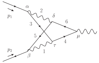
(a)

(b)

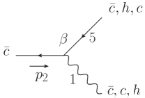
(c)

Figure 7: We show diagram (h) including labels for the vertices and propagators in Fig. 7(a). The vertices $\alpha$ and $\beta$ are shown in Figs. 7(b) and 7(c) with possible momentum modes for each propagator when the loop momenta are regarded as (anti-)collinear.

We finish this appendix by presenting a method that can be used to find all the regions in momentum space of a Feynman integral. In principle, we can use Asy.m to find the scale of each propagator in a given region and then obtain the corresponding modes of loop momenta. However, in our case, it is important to apply an independent cross-check to find the regions in momentum space. To illustrate our method, we focus again on the integral $\mathcal{I}^{X}$, Eq. (B), and use the collinear-type region – which means the loop momenta $k_{1}$ and $k_{2}$ are both collinear or anti-collinear – as an example.

Regardless of whether we perform expansion by region or not, the momentum flowing into a vertex of a Feynman diagram is conserved. We can use this fact to constrain the possible scales of the propagators connected to the same vertex. To make this precise, we labeled the vertices and propagators of $\mathcal{I}^{X}$ in Fig. 7(a). Vertex $\alpha$, shown again in Fig. 7(b), includes three lines with one of them being the external fermion line with momentum $p_{1}$ which is regarded as the collinear momentum. At present, we only focus on the collinear-type regions such that the momentum of one of the remaining two lines should be collinear or anti-collinear. By momentum conservation, the momentum of the third line is now fixed. That is, if the photon line – labeled by 2 – has momentum with collinear scaling, then by momentum conservation the fermion line – labeled by 3 – has also collinear momentum. However, if the photon line has anti-collinear scaling, then the momentum of the fermion line should be hard. The only case left for the collinear-type region is when the fermion line has anti-collinear scaling, which leads to a hard momentum scaling for the photon line. In Fig. 7(c), all possibilities are listed for vertex $\beta$, which attaches to the fermion line with momentum $p_{2}$, regarded as the anti-collinear momentum.

We notice that once we determine the modes of the momenta that flow into the vertices $\alpha$ and $\beta$, the momentum scaling of every line in the diagram can be extracted. As discussed above, the momenta of the lines labelled 2 and 3 can have the modes $cc$, $\bar{c}h$ and $h\bar{c}$ and the momenta of the lines labelled 1 and 5 can have modes $\bar{c}\bar{c}$, $ch$ and $hc$. Naively, we have 9 different configurations after considering these two vertices. We divide these 9 configurations into 3 categories, which are given by

$$R_{1}^{c} =\left(\bar{c}cc\bar{c},\bar{c}\bar{c}h\bar{c},ccch,c\bar{c}hh\right),$$

$$R_{2}^{c} =\left(\bar{c}h\bar{c}\bar{c},hccc,hh\bar{c}c\right),$$

$$R_{3}^{c} =\left(ch\bar{c}h,h\bar{c}hc\right).$$ (152)

Each configuration, e.g. $\bar{c}cc\bar{c}$ in $R_{1}^{c}$, represents the momentum modes of the lines labelled $1$, $2$, $3$ and $5$ respectively. Note that the regions determined by the configurations in $R_{1}^{c}$ can be given using the definition of Eq. (33), while those in $R_{2}^{c}$ can be given using Eq. (39). We did not show the definitions of the propagators that can be used to give the configurations in $R_{3}^{c}$. The reason is that these two configurations in $R_{3}^{c}$ only give scaleless integrals and hence do not contribute. It is also straightforward to check that the integrals in both configurations $c\bar{c}hh$ and $hh\bar{c}c$ are scaleless. Finally, we find 5 contributing configurations, $\bar{c}cc\bar{c}$, $\bar{c}\bar{c}h\bar{c}$, $ccch$, $\bar{c}h\bar{c}\bar{c}$ and $hccc$ which indeed correspond to the $\bar{c}c$, $\bar{c}\bar{c}$, $cc$, $\bar{c}\bar{c}^{\prime}$ and $cc^{\prime}$ regions given in Sec. 5.3, respectively. In principle, one can also choose vertices $\alpha$ and $\mu$ or $\beta$ and $\mu$ to analyze the possible collinear-type regions in topology $X$. However, we did not find any additional collinear-type regions that contributed up to NLP. The other regions in topology $X$, where the loop momenta have hard or ultra-(anti-)collinear scaling, can be found following a similar procedure.