Exploring CP violation in $\boldsymbol{H\to\tau^{+}\,\tau^{-}\,\gamma}$

Abstract

We propose a method of measuring the CP-odd part of the Yukawa interaction of Higgs boson and $\tau$ leptons by observing the forward-backward asymmetry in the decay $H\to\tau^{+}\,\tau^{-}\,\gamma$. The source of such asymmetry is the interference of the CP-even loop-level contribution coming from $H\to Z\,\gamma\to\tau^{+}\,\tau^{-}\,\gamma$ decay channel with the contribution from tree-level CP-odd Yukawa interaction. We find that the CP violating effect is maximum when the invariant mass of the $\tau^{+}\,\tau^{-}$ pair is equal to the mass of the $Z$ boson. We propose and utilise various Dalitz plot asymmetries to quantify the maximal size of the asymmetry and perform Monte Carlo simulations to study the feasibility of measuring it in the high luminosity phase of the Large Hadron Collider (HL-LHC).

1 Introduction

In the Standard Model (SM), violation of the CP symmetry is encoded in the CKM matrix. In principle, a Beyond the Standard Model (BSM) physics may have new sources of CP violation. In particular, BSM CP violation in the Yukawa interactions is welcome for electroweak baryogenesis (it is well known that CP violation in the SM is by far too weak for baryogenesis [1, 2, 3]). The most general expression for CP violating $H\psi\psi$ Yukawa interaction can be written in the following form,

$$\mathscr{L}_{H\psi\psi}=-\frac{m_{\psi}}{\varv}\,\overline{\psi}\left(a_{\psi}+i\,\gamma^{5}\,b_{\psi}\right)\psi\,H\,,$$ (1.1)

where $\varv$ is the vacuum expectation value of the Higgs field, $m_{\psi}$ denotes the mass of the fermion $\psi$, and $a_{\psi},b_{\psi}$ are two real valued parameters. In the SM, $a_{\psi}^{\textrm{SM}}=1$, $b_{\psi}^{\textrm{SM}}=0$. If simultaneously both $a_{\psi}\neq 0$ and $b_{\psi}\neq 0$, it implies CP violation in $H\psi\psi$ Yukawa interaction. The parameters $b_{\psi}$ are strongly constrained by the experimental bounds on the electron and neutron Electric Dipole Moments (for a recent analysis see [4] and references therein). In this context, the $\tau$ lepton Yukawa coupling is of interest as it is large and the EDM bound, $b_{\tau}<0.3$, is weak enough for the $\tau$ Yukawa to play a role in electroweak baryogenesis, see e.g. [5]. CP violation in the $\tau$ Yukawa has also been searched for at the LHC. The recent study by CMS [6] probing $H\to\tau^{+}\,\tau^{-}$ gives $\left|b_{\tau}\right|\lesssim 0.34$ at $68.3\%$ confidence level (for further prospects see [7]). Majority of the experimental studies on this issue concentrate on measurements of the angle between $\tau$ decay planes determined by the directions of particles produced in subsequent $\tau$ lepton decays, such as in $H\to\tau^{+}\,\tau^{-}\to\pi^{+}\,\pi^{-}\,\nu_{\tau}\,\bar{\nu}_{\tau}$ or $H\to\tau^{+}\,\tau^{-}\to\rho^{+}\,\rho^{-}\,\nu_{\tau}\,\bar{\nu}_{\tau}$ [8, 6, 9, 10, 11, 12, 13, 14, 15].

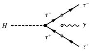
(a) $H\tau\tau$ Yukawa contribution at tree-level. The empty circles denote the fact that the final photon can arise from either of the $\tau$ legs.

(b) $Z\gamma$ and $\gamma\gamma$ contributions from triangular top loop.

(c) $Z\gamma$ and $\gamma\gamma$ contribution from triangular $W$ loop.

(d) $Z\gamma$ and $\gamma\gamma$ contribution from $W$ loop with $WW\gamma Z/\gamma$ vertex.

Figure 1: The dominant Feynman diagrams contributing to $H\to\tau^{+}\,\tau^{-}\,\gamma$. The contributions of possible box diagrams at one-loop level (not shown here) are negligible, see Refs. [16, 17].

In this paper we propose to measure the forward-backward asymmetry of $\tau$ lepton angular distribution in the $H\to\tau^{+}\,\tau^{-}\,\gamma$ decay, as a measure of the CP violation in $H\tau\tau$ Yukawa interaction. To study this asymmetry we utilise the Lorentz invariant Dalitz plot distribution of events. The dominant CP-violating effects which contribute to the forward-backward asymmetry in the $H\to\tau^{+}\,\tau^{-}\,\gamma$ decay are proportional to the interference of the tree-level and loop-level diagrams shown in Fig. 1. The lower branching ratio than the $H\to\tau^{+}\,\tau^{-}$ is partially compensated by the fact that one only requires to reconstruct the 4-momenta of the $\tau$ leptons and not the full spatial distributions of the final $\tau$ decay products. Our heuristic simulations for the HL-LHC show that one can possibly probe $b_{\tau}$ using our proposed methodology. A more thorough Monte Carlo study scanning the full 2-dimensional Dalitz plot distribution is beyond our current expertise, and is hence reserved for future exploration.

Our paper is organised as follows. In Sec. 2 we briefly outline the important phenomenological aspects of the 3-body decay $H\to\tau^{+}\,\tau^{-}\,\gamma$, showing how the forward-backward asymmetry originates and how can it be probed from the Lorentz invariant Dalitz plot distribution. In Sec. 3 we do a numerical study, looking at the distribution pattern inside the Dalitz plot and assess how large the forward-backward asymmetry could be. In Sec. 4 we perform a heuristic Monte Carlo study of the feasibility of observing the asymmetry in context of HL-LHC. Finally we conclude in Sec. 5 summarising our findings and highlighting the salient features of our proposed methodology.

2 Phenomenological study of $\boldsymbol{H\to\tau^{+}\,\tau^{-}\,\gamma}$

The decay $H\to\tau^{+}\,\tau^{-}\,\gamma$ is its own CP-conjugate process. Let us study the kinematic configuration of the decay in the center-of-momentum frame of $\tau^{+}\,\tau^{-}$ (equivalently called the di-tau rest frame). From Fig. 2 it is clear that the CP transformation takes the angle $\theta$ between $\tau^{+}$ and photon to $\pi-\theta$. This implies that any difference (or asymmetry) in the angular distribution of events with respect to $\cos\theta\leftrightarrow-\cos\theta$ (‘forward’ $\leftrightarrow$ ‘backward’) exchange would be a clear signature of CP-violation.

Figure 2: Kinematic configurations related by CP in the center-of-momentum frame of $\tau^{+}\,\tau^{-}$.

As illustrated in Fig. 1 the decay $H\to\tau^{+}\,\tau^{-}\,\gamma$ proceeds via the tree-level $H\tau\tau$ Yukawa interaction, as well as via the effective vertex of $H\to\mathcal{V}\,\gamma\to\tau^{+}\,\tau^{-}\,\gamma$, with $\mathcal{V}=Z,\gamma$. The effective Lagrangian for the later interaction can be, to the lowest mass dimension order, written in the form,

$$\mathscr{L}_{H\mathcal{V}\gamma}=\frac{H}{4\,\varv}\left(2A_{2}^{Z\gamma}F^{\mu\nu}Z_{\mu\nu}+2A_{3}^{Z\gamma}F^{\mu\nu}\widetilde{Z}_{\mu\nu}+A_{2}^{\gamma\gamma}F^{\mu\nu}F_{\mu\nu}+A_{3}^{\gamma\gamma}F^{\mu\nu}\widetilde{F}_{\mu\nu}\right),$$ (2.1)

where $\mathcal{V}_{\mu\nu}=\partial_{\mu}\mathcal{V}_{\nu}-\partial_{\nu}\mathcal{V}_{\mu}$, $\widetilde{\mathcal{V}}_{\mu\nu}=\frac{1}{2}\epsilon_{\mu\nu\rho\sigma}\mathcal{V}^{\rho\sigma}$, and $A_{2,3}^{\mathcal{V}\gamma}$ are dimensionless form factors. Such form factors receive contributions from the SM loop-level diagrams (see Fig. 1), and from the interaction beyond the SM, the latter in general possibly also containing CP-violating couplings. We take into account only the SM loop contributions, assuming that BSM loop corrections are small compared to the tree level ones. Thus, we put $A_{3}^{\mathcal{V}\gamma}=0$ while doing numerical study, but for completeness we will keep the $A_{3}^{\mathcal{V}\gamma}$ dependent terms in our analytical expressions. The expressions for $A_{2}^{Z\gamma}$ and $A_{2}^{\gamma\gamma}$ in the SM are given in Ref. [20].

Let us denote the decay amplitude for $H\to\tau^{+}\,\tau^{-}\,\gamma$ by $\mathscr{M}$. As illustrated in Fig. 1, the amplitude can be split into three parts: (1) tree-level contribution $\mathscr{M}^{\textrm{(Yuk)}}$, (2) loop-level $Z\gamma$ contribution $\mathscr{M}^{(Z\gamma)}$, and (3) loop-level $\gamma\gamma$ contribution $\mathscr{M}^{(\gamma\gamma)}$, i.e. $\mathscr{M}=\mathscr{M}^{\textrm{(Yuk)}}+\mathscr{M}^{(Z\gamma)}+\mathscr{M}^{(\gamma\gamma)}$. Like any other 3-body decay of a spin-0 particle, the full kinematics of $H(p_{H})\to\tau^{+}(p_{+})\,\tau^{-}(p_{-})\,\gamma(p_{0})$ can be described by two independent variables. We choose to work with Lorentz invariant mass squares. Defining

$$m_{+-}^{2} =\left(p_{+}+p_{-}\right)^{2}=\left(p_{H}-p_{0}\right)^{2},$$ (2.2a)

$$m_{+0}^{2} =\left(p_{+}+p_{0}\right)^{2}=\left(p_{H}-p_{-}\right)^{2},$$ (2.2b)

$$m_{-0}^{2} =\left(p_{-}+p_{0}\right)^{2}=\left(p_{H}-p_{+}\right)^{2},$$ (2.2c)

where

$$m_{+-}^{2}+m_{+0}^{2}+m_{-0}^{2}=m_{H}^{2}+2\,m_{\tau}^{2}.$$ (2.3)

We can express $\cos\theta$, defined in the di-tau rest frame, in terms of the Lorentz invariant variables:

$$\cos\theta=\left(1-\dfrac{4\,m_{\tau}^{2}}{m_{+-}^{2}}\right)^{-\frac{1}{2}}\,\frac{m_{-0}^{2}-m_{+0}^{2}}{m_{H}^{2}-m_{+-}^{2}}\,.$$ (2.4)

At the beginning of this section we have argued that the forward-backward asymmetry in $\cos\theta$ distribution can serve as a probe of CP violation. Therefore, we see that the forward-backward asymmetry would be equivalent to an asymmetry in the distribution or number of events in the $m_{+0}^{2}$ vs. $m_{-0}^{2}$ plane (usually called a Dalitz plot) under the exchange $m_{+0}^{2}\leftrightarrow m_{-0}^{2}$. Equivalently, one can consider distribution of events in the $m_{+0}$ vs. $m_{-0}$ plane which may be more convenient from experimental perspective. The ‘forward’ (or ‘backward’) region in Dalitz plot is that region where $m_{-0}>m_{+0}$ (or $m_{-0}<m_{+0}$).

In the rest frame of the Higgs boson, the differential decay rate of $H\to\tau^{+}\,\tau^{-}\,\gamma$ in terms of $m_{+0}$ and $m_{-0}$ is given by,

$$\dfrac{\mathrm{d}^{2}\Gamma_{\tau\tau\gamma}}{\mathrm{d}m_{+0}\,\mathrm{d}m_{-0}}=\frac{m_{+0}\,m_{-0}}{64\,\pi^{3}\,m_{H}^{3}}\left|\mathscr{M}\right|^{2}\equiv\mathcal{D}\big{(}m_{+0},m_{-0}\big{)},$$ (2.5)

where the squared amplitude $\left|\mathscr{M}\right|^{2}$ can be split into six constituents,

$$\left|\mathscr{M}\right|^{2} =\big{|}\mathscr{M}^{(\textrm{Yuk})}\big{|}^{2}+\big{|}\mathscr{M}^{(Z\gamma)}\big{|}^{2}+\big{|}\mathscr{M}^{(\gamma\gamma)}\big{|}^{2}+2\,\textrm{Re}\left(\mathscr{M}^{(\gamma\gamma)}\,\mathscr{M}^{(Z\gamma)*}\right)$$

$$\quad+2\,\textrm{Re}\left(\mathscr{M}^{(\textrm{Yuk})}\,\mathscr{M}^{(Z\gamma)*}\right)+2\,\textrm{Re}\left(\mathscr{M}^{(\textrm{Yuk})}\,\mathscr{M}^{(\gamma\gamma)*}\right).$$ (2.6)

In order to clearly point out the terms responsible for the forward-backward asymmetry and see how it is related to CP-asymmetry, we write down the expression for the individual constituents of amplitude square, as shown in Eq. (2.6), in terms of $m_{+-}^{2}$ and $\theta$. Using Eqs. (2.3) and (2.4) one can easily rewrite all these expressions in terms of $m_{+0}$ and $m_{-0}$. Neglecting the subdominant $m_{\tau}$ dependent terms in the numerator, we have:

$$\big{|}\mathscr{M}^{(\textrm{Yuk})}\big{|}^{2} =\frac{16\,e^{2}\,\left(a_{\tau}^{2}+b_{\tau}^{2}\right)\,m_{\tau}^{2}\,\left(m_{H}^{4}+m_{+-}^{4}\right)\,m_{+-}^{4}\,\sin^{2}\theta}{\varv^{2}\left(m_{H}^{2}-m_{+-}^{2}\right)^{2}\,\left(\left(m_{+-}^{2}-4\,m_{\tau}^{2}\right)\,\sin^{2}\theta+4\,m_{\tau}^{2}\right)^{2}},$$ (2.7a)

$$\big{|}\mathscr{M}^{(Z\gamma)}\big{|}^{2} =\frac{g_{Z}^{2}\,\left(\left(c_{A}^{\tau}\right)^{2}+\left(c_{V}^{\tau}\right)^{2}\right)\,\left(\left(A_{2}^{Z\gamma}\right)^{2}+\left(A_{3}^{Z\gamma}\right)^{2}\right)m_{+-}^{2}\left(m_{H}^{2}-m_{+-}^{2}\right)^{2}}{8\varv^{2}\left(\left(m_{+-}^{2}-m_{Z}^{2}\right)^{2}+\Gamma_{Z}^{2}m_{Z}^{2}\right)}\left(1+\cos^{2}\theta\right),$$ (2.7b)

$$\big{|}\mathscr{M}^{(\gamma\gamma)}\big{|}^{2} =\frac{e^{2}\left(\left(A_{2}^{\gamma\gamma}\right)^{2}+\left(A_{3}^{\gamma\gamma}\right)^{2}\right)\left(m_{H}^{2}-m_{+-}^{2}\right)^{2}}{2\,m_{+-}^{2}\,\varv^{2}}\left(1+\cos^{2}\theta\right),$$ (2.7c)

$$\textrm{Re}\left(\mathscr{M}^{(\gamma\gamma)}\,\mathscr{M}^{(Z\gamma)*}\right) =-\frac{e\,g_{Z}\,\left(m_{H}^{2}-m_{+-}^{2}\right)^{2}}{4\varv^{2}\left(\left(m_{+-}^{2}-m_{Z}^{2}\right)^{2}+\Gamma_{Z}^{2}m_{Z}^{2}\right)}$$

$$\quad\times\Bigg{(}2\,c_{A}^{\tau}\,\left(A_{2}^{\gamma\gamma}A_{3}^{Z\gamma}-A_{2}^{Z\gamma}A_{3}^{\gamma\gamma}\right)\,m_{Z}\,\Gamma_{Z}\,\cos\theta\,$$

$$\qquad+c_{V}^{\tau}\,\left(A_{2}^{\gamma\gamma}A_{2}^{Z\gamma}+A_{3}^{\gamma\gamma}A_{3}^{Z\gamma}\right)\,\left(m_{+-}^{2}-m_{Z}^{2}\right)\left(1+\cos^{2}\theta\right)\Bigg{)},$$ (2.7d)

$$\textrm{Re}\left(\mathscr{M}^{(\textrm{Yuk})}\,\mathscr{M}^{(Z\gamma)*}\right) =\frac{4\,e\,g_{Z}\,m_{\tau}^{2}\,m_{+-}^{4}\,\sin^{2}\theta}{\varv^{2}\left(\left(m_{+-}^{2}-m_{Z}^{2}\right)^{2}+\Gamma_{Z}^{2}m_{Z}^{2}\right)\left(\left(m_{+-}^{2}-4\,m_{\tau}^{2}\right)\,\sin^{2}\theta+4\,m_{\tau}^{2}\right)^{2}}$$

$$\quad\times\Bigg{(}c_{A}^{\tau}\,\left(A_{3}^{Z\gamma}a_{\tau}-A_{2}^{Z\gamma}b_{\tau}\right)\,m_{Z}\,\Gamma_{Z}\,\left(m_{H}^{2}-m_{+-}^{2}\right)\,\cos\theta$$

$$\qquad+c_{V}^{\tau}\left(m_{+-}^{2}-m_{Z}^{2}\right)\bigg{(}A_{2}^{Z\gamma}a_{\tau}\left(m_{H}^{2}-m_{+-}^{2}\cos^{2}\theta\right)$$

$$\hskip 142.26378pt+A_{3}^{Z\gamma}b_{\tau}\left(m_{H}^{2}-m_{+-}^{2}\right)\bigg{)}\Bigg{)},$$ (2.7e)

$$\textrm{Re}\left(\mathscr{M}^{(\textrm{Yuk})}\,\mathscr{M}^{(\gamma\gamma)*}\right) =-\frac{8\,e^{2}\,m_{\tau}^{2}\,m_{+-}^{2}\,\sin^{2}\theta}{\varv^{2}\,\left(\left(m_{+-}^{2}-4\,m_{\tau}^{2}\right)\,\sin^{2}\theta+4\,m_{\tau}^{2}\right)^{2}}$$

$$\quad\times\left(A_{2}^{\gamma\gamma}a_{\tau}\left(m_{H}^{2}-m_{+-}^{2}\,\cos^{2}\theta\right)+A_{3}^{\gamma\gamma}b_{\tau}\left(m_{H}^{2}-m_{+-}^{2}\right)\right),$$ (2.7f)

where $c_{V}^{\tau}=-1/2+2\,\sin^{2}\theta_{W}$, $c_{A}^{\tau}=-1/2$, and $g_{Z}=e/(\sin\theta_{W}\,\cos\theta_{W})$, with $\theta_{W}$ being the weak mixing angle. Note that we have kept the total width of the $Z$ boson, $\Gamma_{Z}$, because the $Z$ boson can be on-shell in our case.

We are interested in terms that are odd (linear) in $\cos\theta$ (or, using Lorentz invariant variables, odd in the difference $m_{+0}^{2}-m_{-0}^{2}$). Such terms are found to be proportional to $m_{Z}\,\Gamma_{Z}$ as well as the product of CP-even and CP-odd couplings. If we use the narrow-width approximation for the $Z$ boson propagator,

$$\frac{1}{\left(m_{+-}^{2}-m_{Z}^{2}\right)^{2}+\Gamma_{Z}^{2}\,m_{Z}^{2}}\approx\frac{\pi}{m_{Z}\,\Gamma_{Z}}\delta\big{(}m_{+-}^{2}-m_{Z}^{2}\big{)},$$ (2.8)

the $m_{Z}\,\Gamma_{Z}$ factor in the terms linear in $\cos\theta$ cancels out, and it is obvious that maximum CP-violation occurs for $m_{+-}^{2}=m_{Z}^{2}$. Thus, the dominant contribution to the forward-backward asymmetry comes from the events for which invariant mass of the $\tau$ pair is close to the $Z$ boson mass.

It is clear from Eq. (2.7e) that to a good approximation the asymmetry in the $\cos\theta$ distribution probes the combination $(A_{3}^{Z\gamma}a_{\tau}-A_{2}^{Z\gamma}b_{\tau})$. In our numerical study in Sec. 3 we put $A_{3}^{Z\gamma}=0$.

In the following section we illustrate how the distribution pattern in the ‘forward’ and ‘backward’ regions of the Dalitz plot differ due to CP violation (i.e. $b_{\tau}\neq 0$) by studying the following distribution asymmetry,

$$\mathcal{A}\left(m_{+0},m_{-0}\right)=\frac{\big{|}\mathcal{D}\left(m_{+0},m_{-0}\right)-\mathcal{D}\left(m_{-0},m_{+0}\right)\big{|}}{\mathcal{D}\left(m_{+0},m_{-0}\right)+\mathcal{D}\left(m_{-0},m_{+0}\right)}.$$ (2.9)

Additionally, we also study the asymmetry integrated over the region where the invariant mass of the $\tau^{+}\,\tau^{-}$ pair is close to the $Z$ boson mass,

$$A(n)=\frac{\displaystyle\Big{|}\iint\Big{(}\mathcal{D}\big{(}m_{+0}<m_{-0}\big{)}-\mathcal{D}\big{(}m_{+0}>m_{-0}\big{)}\Big{)}\,\Pi(m_{+-},n)\,\mathrm{d}m_{+0}\,\mathrm{d}m_{-0}\Big{|}}{\displaystyle\iint\mathcal{D}\big{(}m_{+0},m_{-0}\big{)}\,\Pi(m_{+-},n)\,\mathrm{d}m_{+0}\,\mathrm{d}m_{-0}},$$ (2.10)

where the function $\Pi\left(m_{+-},n\right)$ defines the cut on the invariant mass of the $\tau^{+}\,\tau^{-}$ pair

$$\Pi\left(m_{+-},n\right)=\begin{cases}1&\textrm{for }\big{|}m_{+-}-m_{Z}\big{|}\,\leqslant n\,\Gamma_{Z},\\ 0&\textrm{otherwise}.\end{cases}$$ (2.11)

The asymmetry $A(n)$ is directly related to the number of events around the $Z$ pole,

$$A(n)=\frac{\left|N_{F}(n)-N_{B}(n)\right|}{N_{F}(n)+N_{B}(n)},$$ (2.12)

where $N_{F/B}(n)$ denote the number of events contained in the forward/backward region which are also contained in the region around $Z$ pole as defined in Eq. (2.11).

3 Numerical study

In this section we do a numerical study of the effect of the CP violating parameter $b_{\tau}$ on the Dalitz plot distribution in $m_{+0}$ vs. $m_{-0}$ plane. Especially we focus on the size of the asymmetries $\mathcal{A}\left(m_{+0},m_{-0}\right)$ and $A(n)$ as defined in Eqs. (2.9) and (2.10). As detailed below, we impose a few kinematic cuts in the Higgs rest frame. In the next section we present the results of a heuristic simple MC simulation as an attempt to be closer to the experimental conditions at the HL-LHC.

We note that by neglecting $m_{\tau}$ in comparison with Higgs mass $m_{H}$, one can constrain (to a very good approximation) the sum $a_{\tau}^{2}+b_{\tau}^{2}$ from the experimentally measured $pp\to H\to\tau^{+}\,\tau^{-}$ cross-section [21], which yields

$$a_{\tau}^{2}+b_{\tau}^{2}\approx 0.93^{+0.14}_{-0.12},$$ (3.1)

where the experimental errors have been added in quadrature.

To avoid infrared divergence, we impose a cut on the photon energy (i.e. specify a minimum energy for the photon) in the Higgs rest frame,

$$E_{\gamma}^{\textrm{cut}}=5~{}\textrm{GeV}.$$ (3.2)

As we discuss later, the actual value of this cut has little impact on the decay branching ratios in the range of the di-$\tau$ invariant mass squared $m_{+-}^{2}$ most sensitive to the CP violation effect. For the sake of reference we note that, with this cut, for the full kinematical range of $m^{2}_{+-}$ the branching ratio of $H\to\tau^{+}\,\tau^{-}\,\gamma$ is $BR_{\tau\tau\gamma}=3.72\times 10^{-3}$. The branching ratio decreases once a cut is imposed on the three relative angles $\theta_{X}$, with $X\in\{+-,+0,-0\}$ (see Fig. 3) among the final particles in the Higgs rest frame. An angular cut $\theta_{X}^{\textrm{cut}}$ specifies the minimum angle among the final particles. For $\theta_{X}^{\textrm{cut}}=5^{\circ}$ we get $BR_{\tau\tau\gamma}=3.24\times 10^{-3}$ which further decreases by approximately $15$% for each $5^{\circ}$ increase in the cut. Both the angular cut $\theta_{X}^{\textrm{cut}}$ and photon energy cut $E_{\gamma}^{\textrm{cut}}$ affect the allowed values of $m_{+0}$ and $m_{-0}$.

Figure 3: A schematic kinematic configuration of $\tau^{+}\,\tau^{-}\,\gamma$ in the Higgs rest frame showing angles subtended by the 3-momenta of the final particles.

In Fig. 4 we see that the differential decay distribution have maxima close to the axes when $m_{\pm 0}^{2}$ approaches $m_{\tau}^{2}$. These peaks are characteristic of the tree-level contribution from Fig. 1. A second peak is also easily discernible in the distributions around $m_{+-}^{2}=m_{Z}^{2}$ as a slightly darker band, and this corresponds to contribution from the on-shell $Z$ contribution, coming from the one-loop level diagrams of Fig. 1. Furthermore, for $b_{\tau}\neq 0$ we do find non-zero forward-backward asymmetry. Also as expected, the distribution asymmetry $\mathcal{A}\left(m_{+0},m_{-0}\right)$ become significantly large around the $Z$-pole region. The distribution asymmetry can be as large as $\sim 1\%$ depending on the values of $a_{\tau}$, $b_{\tau}$ such as for $a_{\tau}=0.950$ and $b_{\tau}=0.20$.

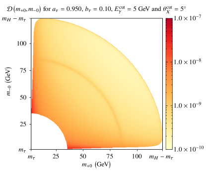
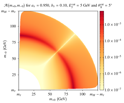
Figure 4: The expected differential decay rates $\mathcal{D}\big{(}m_{+0},m_{-0}\big{)}$ as well as the asymmetry $\mathcal{A}\big{(}m_{+0},m_{-0}\big{)}$ inside the Dalitz plot regions for $a_{\tau}=0.950$, $b_{\tau}=0.1$. The asymmetry is localised around the $Z$ pole as expected (see discussion surrounding Eq. (2.8)). Note that the colour bar is in logarithmic scale.

Regarding the asymmetries $A(n)$ around the $Z$-pole, see Eq. (2.10), we note that the $Z$-pole cut as encoded in Eq. (2.11) can be rewritten, in terms of the photon energy in the Higgs rest frame, as follows,

$$\Pi\big{(}m_{+-},n\big{)}\equiv\Pi\big{(}E_{\gamma},n\big{)}=\begin{cases}1&\textrm{ for }\Big{\lvert}\sqrt{m_{H}^{2}-2\,m_{H}\,E_{\gamma}}-m_{Z}\Big{\rvert}\leqslant n\,\Gamma_{Z},\\ 0&\textrm{ otherwise},\end{cases}$$ (3.3)

From the equation above it is clear that for the invariant mass of the $\tau$ pair close to the $Z$ pole, say $\big{|}m_{+-}-m_{Z}\big{|}\,\leqslant 5\,\Gamma_{Z}$, that the photon energy cut $E_{\gamma}^{\textrm{cut}}=5$ GeV has no relevance, since the minimum photon energy required for events around $Z$-pole corresponds to higher photon energies. Only the angular cuts $\theta_{X}^{\textrm{cut}}$ have any bearing in such a case.

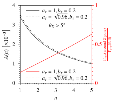
Figure 5: The comparison of forward-backward asymmetry $A(n)$, defined in Eq. (2.12) and the ratio $\Gamma_{\tau\tau\gamma}\textrm{(around $Z$ pole)}/\Gamma_{\tau\tau\gamma}\textrm{(full)}$, where $\Gamma_{\tau\tau\gamma}\textrm{(around $Z$ pole)}$ is the partial decay rates for the decay $H\to\tau^{+}\,\tau^{-}\,\gamma$ with $m_{+-}$ around the $Z$ pole satisfying Eq. (2.11), and $\Gamma_{\tau\tau\gamma}\textrm{(full)}$ is the full partial decay rate.

In Fig. 5 we show the variation of $A(n)$ for $1\leqslant n\leqslant 5$ and compare it with with the ratio $\Gamma_{\tau\tau\gamma}\textrm{(around $Z$ pole)}/\Gamma_{\tau\tau\gamma}\textrm{(full)}$, where $\Gamma_{\tau\tau\gamma}\textrm{(around $Z$ pole)}$ is the partial decay rates for the decay $H\to\tau^{+}\,\tau^{-}\,\gamma$ with $m_{+-}$ around the $Z$ pole (imposed using Eq. (2.11)), and $\Gamma_{\tau\tau\gamma}\textrm{(full)}$ is the full partial decay rate. As expected, the asymmetry decreases with $n$, as it is strongly localised around the $Z$-pole, whereas $\Gamma_{\tau\tau\gamma}\textrm{(around $Z$ pole)}/\Gamma_{\tau\tau\gamma}\textrm{(full)}$ increases with $n$. The plot clearly shows the challenge for an experimental analysis to find an optimal balance between the magnitude of the effect and the statistics of the events.

4 Simulation study of $\boldsymbol{H\to\tau^{+}\,\tau^{-}\,\gamma}$ in the context of HL-LHC

To estimate the sensitivity of the proposed Higgs boson decay $H\to\tau^{+}\,\tau^{-}\,\gamma$ to the CP violation effects at the HL-LHC, Monte-Carlo (MC) generators were used to simulate the signal in the actual experimental environment. However, due to the limited computing resources, we have used a simplified MC simulation procedure. The differential cross-sections corresponding to the various $a_{\tau}$ and $b_{\tau}$ values are computed using GNU Octave [22] as a function of $m_{+0}$ and $m_{-0}$. The MC signal samples are re-weighted using these cross-sections (which include the kinematic cuts of Sec. 3) to properly model the impact of the interference term, similar to the "interpolation" approach used in  [23]. The validity of the approach is verified by the comparison of relevant kinematic distributions with the analytical calculations.

We project the Dalitz plot distribution of events in forward and backward regions onto the $m_{+-}$ axis to do a 1-dimensional binned study of the forward-backward asymmetry. A more detailed and thorough MC study taking the full 2-dimensional Dalitz plot distribution into account and exploring unbinned Dalitz plot analysis techniques such as the Miranda method [24, 25], the method of energy test statistic [26, 27, 28, 29, 30] and the earth mover’s distance [31] are reserved for future explorations.

In the following, all additional cuts are defined in the laboratory frame. Reconstruction of the Higgs rest frame, that was used in the previous section would require the knowledge of the Higgs boson three-momentum which is not known experimentally. Besides, the observed distribution of events in $m_{+0}$ vs. $m_{-0}$ Dalitz plot can be obtained in any frame of reference.

4.1 Monte Carlo Simulation

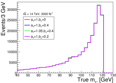
(a) Invariant (true) di-$\tau$ mass.

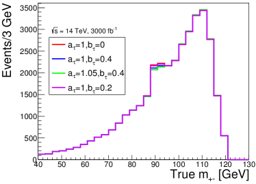
(b) Invariant (true) di-$\tau$ mass after kinematic cuts.

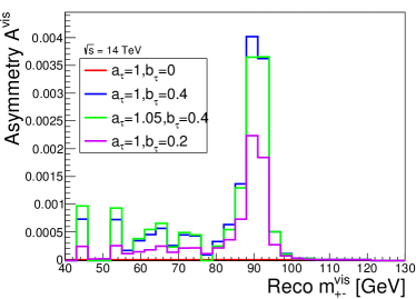
(c) True asymmetry after kinematic cuts.

(d) Visible asymmetry after kinematic cuts.

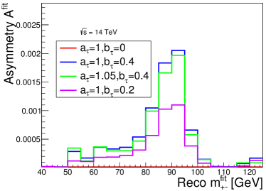
(e) Visible asymmetry after mass refit .

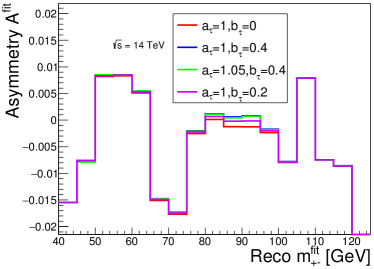
(f) Data-like asymmetry after mass refit.

Figure 6: MC-based predictions of the (a)-(b) invariant mass of the di-$\tau$ system as well as the (c)-(f) asymmetry sensitivity for different values of $a_{\tau}$ and $b_{\tau}$ as a function of di-$\tau$ invariant mass. In (c)-(e) the asymmetry is normalised such that it is always $0$ in the SM, while in (f) the statistical fluctuation of the MC generator are included, with the number of events around 5 times larger than the yields expected at HL-LHC.

For the gluon-fusion production of the Higgs boson, the PowhegBox v2 [32, 33, 34, 35] generator was used with the NNPDF3.0NNLO [36] PDF set. Proton-proton collisions are set to happen at center-of-mass energy of $14$ TeV, as is expected for HL-LHC. For the simulation of the decay of the Higgs boson, modelling of the parton showers, and hadronization, the simulated events were processed with the Pythia v8.306 [37] program with the CTEQ6L1 [38] PDF set. DELPHES 3.5 [39] framework is then used to emulate the resolution and reconstruction of physical objects (such as photons, $\tau$ leptons, and jets) by a general-purpose particle detector (such as ATLAS or CMS) using the "HLLHC" card. FastJet 3.3.4 [40] package is used to perform the jet clustering using the anti-$k_{t}$ algorithm [41].

In the simulation studies photons are required to have $p_{T}>10$ GeV and to be isolated with an angular cone defined by the condition $\Delta R\leq 0.3$. The reconstructed $\tau$ leptons are required to have $p_{T}>15$ GeV. Their reconstruction is based on seed jets with the radius parameter [41] $\textsf{R}=0.4$. This $p_{T}$ selection represents a realistic lower limit of what a general purpose detector can achieve. We assume that hadronically decaying $\tau$ leptons can be identified with $100\%$ efficiency. In reality this efficiency will be heavily dependent on the desired jet rejection power achievable with the conditions of the HL-LHC. The results presented in this section scale trivially with the $\tau$ identification efficiency. This optimisation is left for the future, more realistic, simulations of the performance of $\tau$ identification algorithms at the HL-LHC. All plots in this subsection are based on the MC simulation described above.

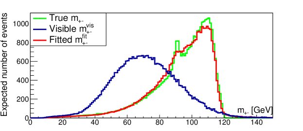
(a) Invariant mass of the di-$\tau$

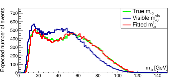
(b) Invariant mass of $\tau^{-}\gamma$

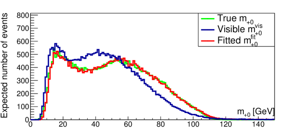
(c) Invariant mass of $\tau^{+}\gamma$

Figure 7: The invariant masses $m_{+-},m_{+0}$ and $m_{-0}$ using true, visible, and fitted physical objects.

The HL-LHC is expected to deliver about $3000$ fb^-1 integrated luminosity of data [42]. This corresponds to over $160$ million events with gluon-gluon fusion production of the Higgs boson. With hadronically reconstructed $\tau$s and taking the same kinematic constraints as considered in Section 3, we estimate that $2.24\times 10^{5}$ of these Higgs bosons will eventually decay into the $\gamma\,\tau^{+}_{\text{had}}\,\tau^{-}_{\text{had}}$ final state. Approximately $10\%$ of the events will have the di-$\tau$ system with the invariant mass $m_{+-}$ within $5$ GeV of the $Z$-boson mass peak where the forward-backward asymmetry manifests, see Fig. 6a. For any selected range of $m_{+-}$ we can estimate the number of events in ‘forward’ and ‘backward’ regions, say $N_{F}$ and $N_{B}$ respectively. Thus we can easily estimate the following forward-backward asymmetry,

$$A=\frac{N_{F}-N_{B}}{N_{F}+N_{B}}\,.$$ (4.1)

The laboratory frame kinematic requirements applied to the reconstructed objects, such as the $\tau$ and photon $p_{T}$ and isolation requirements, further reduce the number of available events by a factor of 3 in the $Z$ mass peak region, see Fig. 6b. The photon $p_{T}$ requirement by itself is responsible for a $50\%$ decrease in the selection efficiency.

4.2 Kinematic Fit

Although the true invariant mass of the di-$\tau$ system ($m_{+-}$) offers a good way to access the forward-backward asymmetry, see Fig. 6c, it is not accessible experimentally. The short lifetime of the $\tau$ leptons means that they will decay before reaching the detector, with $\nu_{\tau}$ escaping undetected. For hadronically decaying taus that are used in the present study, the particles registered in the detector will be predominantly charged and neutral pions. The detectors have limited acceptance and resolution, meaning that energies and momenta of these particles will be reconstructed with a limited accuracy. The visible invariant mass of the di-$\tau$ system ($m_{+-}^{\textrm{vis}}$), constructed from the visible decay products of $\tau$ decays, offers a degraded sensitivity to the forward-backward asymmetry, with almost no visible $Z$ peak, see Fig. 6d. A fit procedure to recover the sensitivity to the asymmetry based on the kinematic constraints of the system is described in the following.

The final state of $H\to\gamma\,\tau^{+}\,\tau^{-}$ is subject to two constraints:

1. The true invariant mass of the three final particles must be equal to the mass of the Higgs boson.

2. The energy in the transverse plane, perpendicular to the beam line, should be conserved and equal to $0$, with any deviations coming from either the missing neutrinos ($\nu_{\tau},\overline{\nu}_{\tau}$) or mismeasurements of the particle’s energies.

A fit procedure using Minuit2 [43] is performed based on these two conditions with the overall energy of the two $\tau$ leptons as free parameters. Since the opening angle between the neutrinos and visible tau decay product has to be of the order of $m_{\tau}/E_{\tau}$, both $\nu_{\tau}$ and $\bar{\nu}_{\tau}$ are predominantly collinear with the visible parts of the hadronically decaying $\tau$’s, for the energies considered here. Therefore, the approach of treating the contributions from the $\tau$ neutrino and $\tau$ energy smearing as one common parameter that only affects the energy of the $\tau$-lepton and not its spacial direction is justified.

This simple fit procedure allows us to restore the true energies of the $\tau$-leptons and the fitted two-body invariant masses match well with the true invariant masses, as demonstrated in Fig. 7. Further the fitted invariant masses $m^{\text{fit}}_{+0}$ and $m^{\text{fit}}_{-0}$ are used to identify events in forward and backward regions. This information is then used to estimate the asymmetry $A^{\text{fit}}$ while selecting $m^{\text{fit}}_{+-}$ in the region around $Z$-boson mass where the asymmetry is maximal. The asymmetry defined using the fitted masses, $A^{\text{fit}}$ behaves similarly as expected for the true asymmetry as a function of the fitted di-$\tau$ mass, see Fig. 6e. Thus $A^{\text{fit}}$ is a reasonable estimator of the forward-backward asymmetry. In the following we evaluate this asymmetry in a real-data-like environment.

4.3 Asymmetry Calculation

We compare two methods of quantifying the asymmetry and estimating the corresponding values of $b_{\tau}$. The first approach uses a simple selection of events with $m^{\text{fit}}_{+-}$ close to the $Z$ mass peak, where the asymmetry is maximised. Here, the window of $\pm 9$ GeV around $m_{Z}$ was chosen, i.e. $\left|m^{\text{fit}}_{+-}-m_{Z}\right|\leqslant 9$ GeV. The width of this window was inspired by the range of the di-tau mass $m^{\text{fit}}_{+-}$ where the asymmetry is enhanced, see Figs. 6e and 6f. The asymmetry estimate $A^{\text{fit}}$ is then computed as in the equation 4.1 and used to predict $b_{\tau}$.

The second approach involves widening the di-$\tau$ mass selection to the range of $72$–$114$ GeV. The asymmetry $A^{\text{fit}}$ is computed in bins of $3$ GeV. A skewed Gaussian $f_{\text{skew}}(t)$ is then fitted to the shape of the asymmetry distribution,

$$f_{\text{skew}}(t)=c\phi(t)\Phi(\alpha t),\qquad t=\frac{x-a}{b},$$ (4.2)

where $\phi(x)$ is the normal probability density function, $\Phi(x)$ is the normal cumulative distribution function, and $a,b,c,\alpha$ are the free parameters in the fit. These parameters are first determined in the fit to the shapes of the true asymmetry distributions obtained from analytical calculations, see Fig. 8a. All parameters except for the overall scaling factor $c$ are then fixed and the skewed Gaussian is fitted to the distribution of $A^{\text{fit}}$, see Fig. 8b. The determined value of $c$ is compared to the values from the fits to the analytical shapes to determine the $b_{\tau}$, as shown in Fig. 8c. For sake of completeness Fig. 8d shows the fit to the reconstructed-fitted di-tau mass distribution for reconstructed events in the SM case when $b_{\tau}=0$.

The results of the two approaches are summarised in Table 1. The uncertainties of the measurements include the statistical uncertainty of the expected HL-LHC event yields, which is the dominant one. To estimate the HL-LHC uncertainty contribution we rescale the yields to match those expected at $3000$fb^-1 and recompute the statistical uncertainty accordingly. Both of the approaches produce comparable central values with the fit to $f_{\text{skew}}$ resulting in lower uncertainties.

$(a_{\tau},b_{\tau})$	$b_{\tau}$ from $\pm 9$ GeV mass window	$b_{\tau}$ from $f_{\text{skew}}(x)$ fit
$(1,0.0)$	$0.22\pm 2.24$	$0.23\pm 2.06$
$(1,0.1)$	$0.32\pm 2.24$	$0.32\pm 2.07$
$(1,0.2)$	$0.41\pm 2.22$	$0.44\pm 2.14$
$(1,0.3)$	$0.53\pm 2.36$	$0.55\pm 2.24$
$(1,0.4)$	$0.65\pm 2.52$	$0.67\pm 2.39$

Table 1: True and predicted values of $b_{\tau}$ from two different methods. Integrated luminosity of $3000$fb^-1 is assumed.

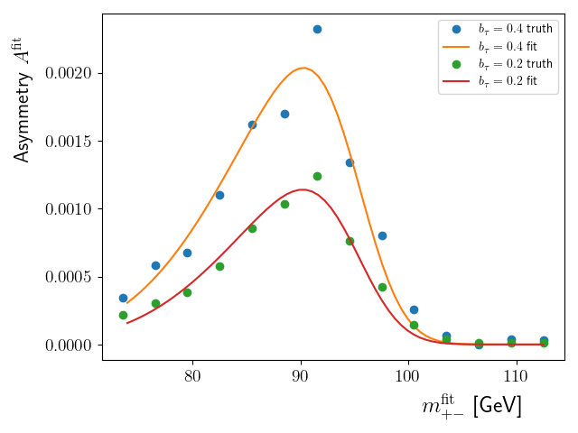
(a) Truth-based asymmetry fits.

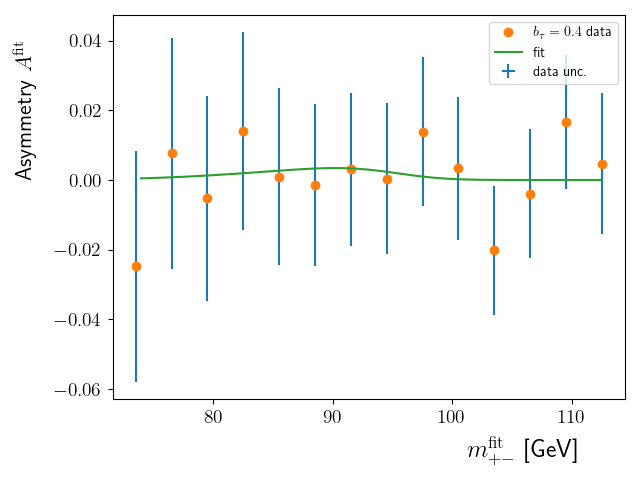
(b) Fit to the reconstructed-fitted mass distribution for reconstructed events, $b_{\tau}=0.4$.

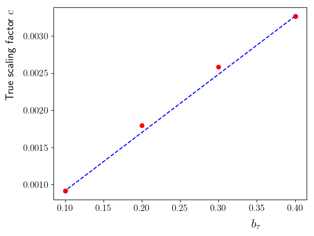
(c) $b_{\tau}$ vs scaling factor $c$.

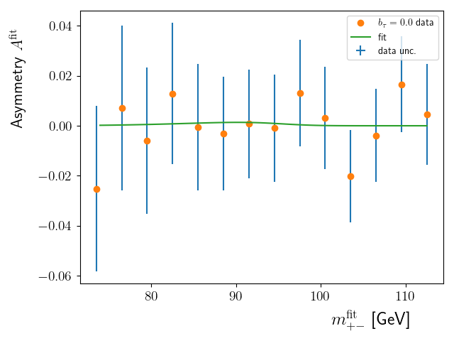
(d) Fit to the reconstructed-fitted mass distribution for reconstructed events, $b_{\tau}=0$.

Figure 8: Gaussian fits to (a) truth-based asymmetry shapes and (b) data-like shapes in MC with $b_{\tau}=0.4$; (c) shows the relationship between true $b_{\tau}$ and the scaling factor $c$ from the fits of analytically computed asymmetry $A$ distributions; (d) data-like shapes in MC with $b_{\tau}=0$ (as is expected in the SM). Note that the uncertainty bars in (b) and (d) represents the statistical uncertainty expected at HL-LHC.

5 Conclusions

We have analysed the 3-body decay of the Higgs boson $H\to\tau^{+}\,\tau^{-}\,\gamma$ as an additional source of information about the CP violation in the $H\tau\tau$ Yukawa coupling, independent from the existing experimental studies on the 2-body decay $H\to\tau^{+}\,\tau^{-}$ [8, 6, 9, 10, 11, 12, 13, 14, 15]. The forward-backward asymmetry in the $\tau$ angular distribution in our case arises due to the interference of the tree-level contribution (which includes the CP violating $H\tau\tau$ Yukawa coupling $b_{\tau}\neq 0$) and the CP-even SM loop-level contributions. We have proposed a novel method of measuring forward-backward asymmetry in the Dalitz plot distribution of events in the plane of $\gamma\,\tau^{\pm}$ Lorentz invariant masses ($m_{+0}$ vs. $m_{-0}$ plane). Such a Dalitz plot distribution is frame independent, making the method of extraction of forward-backward asymmetry clean and attractive from the experimental point of view. The asymmetry is directly proportional to the CP-odd $H\tau\tau$ coupling parameter $b_{\tau}$. In principle, the asymmetry can also appear from the interference of CP-even tree-level contribution and CP violating loop-level contributions. However, for our numerical study, we assume no CP-violation at loop-level and focus only on the effects of non-zero $b_{\tau}$ and whether this can be experimentally probed at HL-LHC.

The forward-backward asymmetry is predicted to be the largest when the di-$\tau$ invariant mass $m_{+-}$ is close to $m_{Z}$ (it could reach $\sim 1\%$ for high values of $b_{\tau}$) and it rapidly diminishes as one moves farther away from the $Z$ pole. To estimate the feasibility of such asymmetry measurements at the HL-LHC we have performed a simplified MC simulation with kinematic cuts meant to mimic the experimental conditions. A kinematic fit was used to constrain the hadronically reconstructed $\tau$-leptons and account for the missing $\nu_{\tau}$ information not available in the detector. We estimated the asymmetry directly in the region with di-$\tau$ mass in the range of $m_{Z}\pm 9$ GeV for different values of $b_{\tau}$. We also looked for the asymmetry by performing a shape fit in a wider mass region, $72~{}\text{GeV}\leqslant m_{+-}\leqslant 114~{}\text{GeV}$.

From our MC studies we find that the statistical uncertainties we currently expect to get with the HL-LHC dataset are significantly larger than the effect itself. Nevertheless, our simplistic MC study suggests that our proposed methodology is experimentally doable, and our results could be encouraging for more detailed and in-depth explorations in the future. Instead of the one-dimensional binned shape fit used in this study a full two-dimensional unbinned Dalitz plot analysis could instead be envisaged using for example the Miranda method [24, 25], the method of energy test statistic [26, 27, 28, 29, 30] and the earth mover’s distance [31]. The asymmetry can also appear from the interference of CP-even tree-level contribution and CP violating loop-level contributions, this effect has not been considered in our numerical studies yet. In our MC simulation, we have only considered final states with both of the $\tau$-leptons decaying hadronically, the dataset can be doubled by also considering one of the $\tau$s to decay leptonically, i.e. adding the $H\to\tau_{\text{had}}\tau_{\text{lep}}\gamma$ decay channel. With the better understanding of the technical capabilities of particle detectors such as ATLAS and CMS after the Phase-2 upgrades, the kinematic selections can be further optimised.

Finally, once the asymmetry can be probed with reduced uncertainty, it would be interesting to compare its prediction for $b_{\tau}$ with that obtained from the already ongoing experimental study of $H\to\tau^{+}\,\tau^{-}\to m^{+}\,\overline{\nu}_{\tau}\,m^{-}\,\nu_{\tau}$ where $m=\pi,\rho$ etc. If there is significant deviation in the two $b_{\tau}$ values, one can assume that there is some significant CP-violation coming from the loop-level contribution, which we have neglected in our numerical study in this paper. It is interesting to note that the same loop-level diagrams also contribute to $H\to\ell^{+}\,\ell^{-}\,\gamma$ for $\ell=e,\mu$, and for these decay modes the tree-level contributions are negligible. Moreover, the same Dalitz plot techniques developed for $H\to\tau^{+}\,\tau^{-}\,\gamma$ can also be applied to probe the asymmetry in the Dalitz plots of $H\to\ell^{+}\,\ell^{-}\,\gamma$ to constrain or discover the CP violation at loop-level. Therefore, our formalism of probing the forward-backward asymmetry inside the Lorentz invariant Dalitz plot distribution of events would certainly help explore CP property of the Higgs boson in a more systematic and unified manner.

References

- [1] M. E. Shaposhnikov, “Baryon Asymmetry of the Universe in Standard Electroweak Theory,” Nucl. Phys. B 287 (1987) 757–775.
- [2] M. B. Gavela, P. Hernandez, J. Orloff, and O. Pene, “Standard model CP violation and baryon asymmetry,” Mod. Phys. Lett. A 9 (1994) 795–810, arXiv:hep-ph/9312215.
- [3] M. B. Gavela, P. Hernandez, J. Orloff, O. Pene, and C. Quimbay, “Standard model CP violation and baryon asymmetry. Part 2: Finite temperature,” Nucl. Phys. B 430 (1994) 382–426, arXiv:hep-ph/9406289.
- [4] E. Fuchs, M. Losada, Y. Nir, and Y. Viernik, “ violation from , and dimension-6 Yukawa couplings - interplay of baryogenesis, EDM and Higgs physics,” JHEP 05 (2020) 056, arXiv:2003.00099 [hep-ph].
- [5] J. Alonso-González, L. Merlo, and S. Pokorski, “A new bound on CP violation in the lepton Yukawa coupling and electroweak baryogenesis,” JHEP 06 (2021) 166, arXiv:2103.16569 [hep-ph].
- [6] CMS Collaboration, A. Tumasyan et al., “Analysis of the structure of the Yukawa coupling between the Higgs boson and leptons in proton–proton collisions at TeV,” JHEP 06 (2022) 012, arXiv:2110.04836 [hep-ex].
- [7] A. V. Gritsan et al., “Snowmass White Paper: Prospects of CP-violation measurements with the Higgs boson at future experiments,” arXiv:2205.07715 [hep-ex].
- [8] ATLAS Collaboration, G. Aad et al., “Test of CP invariance in vector-boson fusion production of the Higgs boson in the channel in proton–proton collisions at TeV with the ATLAS detector,” Phys. Lett. B 805 (2020) 135426, arXiv:2002.05315 [hep-ex].
- [9] CMS Collaboration, A. Tumasyan et al., “Constraints on anomalous Higgs boson couplings to vector bosons and fermions from the production of Higgs bosons using the final state,” Phys. Rev. D 108 no. 3, (2023) 032013, arXiv:2205.05120 [hep-ex].
- [10] S. Berge, W. Bernreuther, and J. Ziethe, “Determining the CP parity of Higgs bosons at the LHC in their tau decay channels,” Phys. Rev. Lett. 100 (2008) 171605, arXiv:0801.2297 [hep-ph].
- [11] S. Berge and W. Bernreuther, “Determining the CP parity of Higgs bosons at the LHC in the tau to 1-prong decay channels,” Phys. Lett. B 671 (2009) 470–476, arXiv:0812.1910 [hep-ph].
- [12] S. Berge, W. Bernreuther, B. Niepelt, and H. Spiesberger, “How to pin down the CP quantum numbers of a Higgs boson in its tau decays at the LHC,” Phys. Rev. D 84 (2011) 116003, arXiv:1108.0670 [hep-ph].
- [13] S. Berge, W. Bernreuther, and H. Spiesberger, “Higgs CP properties using the decay modes at the ILC,” Phys. Lett. B 727 (2013) 488–495, arXiv:1308.2674 [hep-ph].
- [14] R. Harnik, A. Martin, T. Okui, R. Primulando, and F. Yu, “Measuring CP Violation in at Colliders,” Phys. Rev. D 88 no. 7, (2013) 076009, arXiv:1308.1094 [hep-ph].
- [15] K. Hagiwara, K. Ma, and S. Mori, “Probing CP violation in at the LHC,” Phys. Rev. Lett. 118 no. 17, (2017) 171802, arXiv:1609.00943 [hep-ph].
- [16] A. Abbasabadi, D. Bowser-Chao, D. A. Dicus, and W. W. Repko, “Higgs photon associated production at colliders,” Phys. Rev. D 52 (1995) 3919–3928, arXiv:hep-ph/9507463.
- [17] A. Abbasabadi, D. Bowser-Chao, D. A. Dicus, and W. W. Repko, “Radiative Higgs boson decays ,” Phys. Rev. D 55 (1997) 5647–5656, arXiv:hep-ph/9611209.
- [18] Y. Chen, A. Falkowski, I. Low, and R. Vega-Morales, “New Observables for CP Violation in Higgs Decays,” Phys. Rev. D 90 no. 11, (2014) 113006, arXiv:1405.6723 [hep-ph].
- [19] A. Y. Korchin and V. A. Kovalchuk, “Angular distribution and forward–backward asymmetry of the Higgs-boson decay to photon and lepton pair,” Eur. Phys. J. C 74 no. 11, (2014) 3141, arXiv:1408.0342 [hep-ph].
- [20] L. Bergstrom and G. Hulth, “Induced Higgs Couplings to Neutral Bosons in Collisions,” Nucl. Phys. B 259 (1985) 137–155. [Erratum: Nucl.Phys.B 276, 744–744 (1986)].
- [21] ATLAS Collaboration, G. Aad et al., “Measurements of Higgs boson production cross-sections in the decay channel in pp collisions at TeV with the ATLAS detector,” JHEP 08 (2022) 175, arXiv:2201.08269 [hep-ex].
- [22] J. W. Eaton, D. Bateman, S. Hauberg, and R. Wehbring, GNU Octave version 8.2.0 manual: a high-level interactive language for numerical computations, 2023. https://www.gnu.org/software/octave/doc/v8.2.0/.
- [23] ATLAS Collaboration, G. Aad et al., “Search for dark matter in events with missing transverse momentum and a Higgs boson decaying into two photons in pp collisions at TeV with the ATLAS detector,” JHEP 10 (2021) 013, arXiv:2104.13240 [hep-ex].
- [24] I. Bediaga, I. I. Bigi, A. Gomes, G. Guerrer, J. Miranda, and A. C. d. Reis, “On a CP anisotropy measurement in the Dalitz plot,” Phys. Rev. D 80 (2009) 096006, arXiv:0905.4233 [hep-ph].
- [25] BaBar Collaboration, B. Aubert et al., “Search for CP Violation in Neutral D Meson Cabibbo-suppressed Three-body Decays,” Phys. Rev. D 78 (2008) 051102, arXiv:0802.4035 [hep-ex].
- [26] B. Aslan and G. Zech, “New test for the multivariate two-sample problem based on the concept of minimum energy,” Journal of Statistical Computation and Simulation 75 no. 2, (2005) 109–119.
- [27] M. Williams, “Observing CP Violation in Many-Body Decays,” Phys. Rev. D 84 (2011) 054015, arXiv:1105.5338 [hep-ex].
- [28] LHCb Collaboration, R. Aaij et al., “Search for CP violation in decays with the energy test,” Phys. Lett. B 740 (2015) 158–167, arXiv:1410.4170 [hep-ex].
- [29] LHCb Collaboration, R. Aaij et al., “Search for CP violation in the phase space of decays with the energy test,” JHEP 09 (2023) 129, arXiv:2306.12746 [hep-ex].
- [30] LHCb Collaboration, R. Aaij et al., “Search for CP violation in the phase space of decays with the energy test,” arXiv:2310.19397 [hep-ex].
- [31] A. Davis, T. Menzo, A. Youssef, and J. Zupan, “Earth mover’s distance as a measure of CP violation,” JHEP 06 (2023) 098, arXiv:2301.13211 [hep-ph].
- [32] S. Frixione and B. R. Webber, “Matching NLO QCD computations and parton shower simulations,” JHEP 06 (2002) 029, arXiv:hep-ph/0204244.
- [33] S. Alioli, P. Nason, C. Oleari, and E. Re, “A general framework for implementing NLO calculations in shower Monte Carlo programs: the POWHEG BOX,” JHEP 06 (2010) 043, arXiv:1002.2581 [hep-ph].
- [34] P. Nason, “A New method for combining NLO QCD with shower Monte Carlo algorithms,” JHEP 11 (2004) 040, arXiv:hep-ph/0409146.
- [35] J. M. Campbell, R. K. Ellis, R. Frederix, P. Nason, C. Oleari, and C. Williams, “NLO Higgs Boson Production Plus One and Two Jets Using the POWHEG BOX, MadGraph4 and MCFM,” JHEP 07 (2012) 092, arXiv:1202.5475 [hep-ph].
- [36] C. Anastasiou, L. J. Dixon, K. Melnikov, and F. Petriello, “High precision QCD at hadron colliders: Electroweak gauge boson rapidity distributions at NNLO,” Phys. Rev. D 69 (2004) 094008, arXiv:hep-ph/0312266.
- [37] C. Bierlich et al., “A comprehensive guide to the physics and usage of PYTHIA 8.3” arXiv:2203.11601 [hep-ph].
- [38] J. Pumplin, D. R. Stump, J. Huston, H. L. Lai, P. M. Nadolsky, and W. K. Tung, “New generation of parton distributions with uncertainties from global QCD analysis,” JHEP 07 (2002) 012, arXiv:hep-ph/0201195.
- [39] DELPHES 3 Collaboration, J. de Favereau, C. Delaere, P. Demin, A. Giammanco, V. Lemaître, A. Mertens, and M. Selvaggi, “DELPHES 3, A modular framework for fast simulation of a generic collider experiment,” JHEP 02 (2014) 057, arXiv:1307.6346 [hep-ex].
- [40] M. Cacciari, G. P. Salam, and G. Soyez, “FastJet User Manual,” Eur. Phys. J. C 72 (2012) 1896, arXiv:1111.6097 [hep-ph].
- [41] M. Cacciari, G. P. Salam, and G. Soyez, “The anti- jet clustering algorithm,” JHEP 04 (2008) 063, arXiv:0802.1189 [hep-ph].
- [42] I. Zurbano Fernandez et al., “High-Luminosity Large Hadron Collider (HL-LHC): Technical design report,” CERN Yellow Reports: Monographs, CERN-2020-010 10/2020 (12, 2020) .
- [43] F. James and M. Roos, “Minuit: A System for Function Minimization and Analysis of the Parameter Errors and Correlations,” Comput. Phys. Commun. 10 (1975) 343–367.