MACE: A Multi-pattern Accommodated and Efficient Anomaly Detection Method in the Frequency Domain

Abstract

Anomaly detection significantly enhances the robustness of cloud systems. While neural network-based methods have recently demonstrated strong advantages, they encounter practical challenges in cloud environments: the contradiction between the impracticality of maintaining a unique model for each service and the limited ability to deal with diverse normal patterns by a unified model, as well as issues with handling heavy traffic in real time and short-term anomaly detection sensitivity. Thus, we propose MACE, a Multi-pattern Accommodated and efficient Anomaly detection method in the frequency domain for time series anomaly detection. There are three novel characteristics of it: (i) a pattern extraction mechanism excelling at handling diverse normal patterns, which enables the model to identify anomalies by examining the correlation between the data sample and its service normal pattern, instead of solely focusing on the data sample itself; (ii) a dualistic convolution mechanism that amplifies short-term anomalies in the time domain and hinders the reconstruction of anomalies in the frequency domain, which enlarges the reconstruction error disparity between anomaly and normality and facilitates anomaly detection; (iii) leveraging the sparsity and parallelism of frequency domain to enhance model efficiency. We theoretically and experimentally prove that using a strategically selected subset of Fourier bases can not only reduce computational overhead but is also profitable to distinguish anomalies, compared to using the complete spectrum. Moreover, extensive experiments demonstrate MACE’s effectiveness in handling diverse normal patterns with a unified model and it achieves state-of-the-art performance with high efficiency.

I Introduction

Anomaly detection is a widely studied problem that plays a pivotal role in enhancing the reliability of cloud systems [1]. Current research efforts in this area can be broadly categorized into four distinct groups: classical machine learning-based methods [2, 3, 4], statistical methods [5, 6, 7], signal analysis-based approaches [8, 9, 10], and deep learning-based techniques [11, 12, 13]. Classical machine learning-based methods and statistical methods offer computational efficiency but often rely on specific assumptions, making them not always robust in highly variable scenarios, such as those encountered in the cloud environment [14]. Signal analysis-based methods struggle to capture both global and subtle features simultaneously while maintaining manageable computational overhead [14]. In contrast, deep learning-based methods exhibit a strong advantage in adapting to variable environments. Among them, many reconstruction-based methods have achieved state-of-the-art performance in anomaly detection.

While there have been notable advancements in reconstruction-based methods, several pivotal challenges persist, as outlined below:

• Limited Capability to Capture Diverse Normal Patterns with a Unified Model: It is reported that many reconstruction-based methods can only effectively capture one type of normal pattern for each trained model [15]. However, in practical scenarios, cloud centers host millions of services concurrently, and each service exhibits a unique normal pattern. The challenge arises from the impracticality and excessive cost associated with maintaining a separate model for each individual service. This discrepancy between the experimental setting and the real-world complexity underscores the need for a multi-pattern accommodated approach in the realm of reconstruction-based anomaly detection.

• Shortcomings in Handling Heavy Traffic in Real Time: In large cloud centers, the volume of service traffic can escalate to hundreds of thousands of requests per second. In these high-demand scenarios, numerous deep learning-based methods face challenges in efficiently handling peak traffic in real time. Furthermore, a notable complication arises from the incorporation of recurrent networks in several anomaly detection neural networks, such as VRNN [16], omniAnomaly [17], and MSCRED [18]. This inclusion hampers operator parallelization, as recurrent networks cannot be effectively parallelized across different recurrent steps.

• Insensitivity to Single Point Anomalies: Encoder-decoder neural networks, which are used by many reconstruction-based methods, are insensitive to short-term anomalies and often overlook them [19, 20].

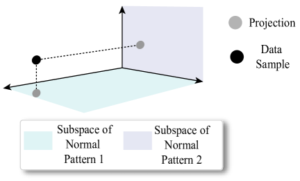
(a) An intuitive illustration for pattern extraction mechanism.

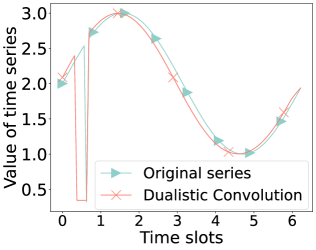
(b) Dualistic convolution in the time domain.

Figure 1: (a) A data sample is projected to a normal pattern subspace in pattern extraction mechanism. When the data sample is closer to the normal pattern subspace, it is easier to reconstruct it from its projection with less reconstruction error. Thus, the data sample is more likely to be inferred as normality for the normal pattern 1 than normal pattern 2. (b) The dualistic convolution applying to the time domain actually extends the short-term anomalies.

Tackling these challenges is imperative for enhancing the efficacy and applicability of deep learning-based anomaly detection methods in practical cloud environments. Therefore, we design innovative mechanisms to address these issues, as outlined below:

• To enhance the model’s ability to accommodate diverse normal patterns (C1), we propose a pattern extraction mechanism. The most challenging problem of dealing with diverse normal patterns is that an anomaly for one normal pattern could be a normality for another. Thus, we detect anomalies according to the correlation between the data sample and its service normal pattern, instead of the data sample itself. The pattern extraction mechanism identifies a normal pattern subspace in the frequency domain for each service. Subsequently, it tailors a representation for each data sample from the sample’s projection on its service normal pattern subspace. In this way, when the data sample is closer to its service normality subspace, it is easier to reconstruct from the representation with less reconstruction error and is more likely to be inferred as normality, as shown in Fig. 1(a).

• To enhance the model’s efficiency and parallelism (C2), we develop a frequency-domain-based method. Detecting anomalies in the frequency domain can leverage sparsity to reduce computational overhead and improve fine-grained parallelism by eliminating temporal dependencies. To leverage the sparsity of the frequency domain, we provide a strategy to select a subset of Fourier bases for each service in the pattern extraction mechanism and theoretically prove that only using the subset of Fourier bases can not only reduce the computational overhead but also improve the anomaly detection performance, compared with using the complete spectrum. To effectively detect anomalies in the frequency domain, we propose a dualistic convolution mechanism to replace the vanilla convolution in the auto-encoder, which hinders the reconstruction of anomalies and keeps the reconstruction of normalities easy.

• To enhance the sensitivity to short-term anomalies (C3), we introduce the dualistic convolution mechanism to the time domain, which amplifies the anomalies, facilitating their detection. As illustrated in Fig. 1(b), the dualistic convolution mechanism extends anomalies while maintaining the similarity of normality to the original time series.

Accordingly, this work makes the following novel and unique contributions to the field of anomaly detection:

• We propose a novel pattern extraction mechanism to deal with diverse normal patterns by facilitating the model to detect anomalies from the correlation between the data sample and its service normal pattern, instead of only the data sample.

• We propose a dualistic convolution mechanism. In the time domain, it amplifies the anomalies. In the frequency domain, it hinders the reconstruction of anomalies while keeping the reconstruction of normalities easy.

• We leverage the sparsity and parallelism of the frequency domain to improve model efficiency. It is theoretically and experimentally proved that using just a subset of Fourier bases can not only reduce computational overhead but also achieve better anomaly detection performance compared with using the complete spectrum.

Moreover, we conduct extensive experiments on four real-world datasets to demonstrate that MACE is multi-pattern accommodated and achieves state-of-the-art performance with high efficiency.

II Proposed Method

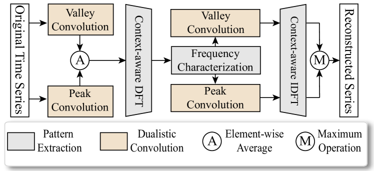
Figure 2: The model architecture of MACE

II-A Overview

TABLE I: The definition of symbols.

Symbol	Definition
$\gamma$	The power in dualistic convolution
$\sigma$	The scaling factor in dualistic convolution
$s$	The stride length of convolution
$\omega_{i}$	The frequency of $i^{th}$ strongest signal of normal pattern
$\mathcal{A}_{N}(\omega_{i})$	The amplitude of normality spectrum corresponding to $\omega_{i}$
$\mathcal{A}_{A}(\omega_{i})$	The amplitude of anomaly spectrum corresponding to $\omega_{i}$
$q_{N}(\omega_{i})$	The normalized value of $\mathcal{A}_{N}(\omega_{i})$
$q_{A}(\omega_{i})$	The normalized value of $\mathcal{A}_{A}(\omega_{i})$
$\mathcal{A}_{i}$	The $i^{th}$ amplitude of a spectrum
$\Delta\mathcal{A}_{i}$	The shift variable adding to normal spectrum
$\Delta A$	The expectation of shift variable
$\alpha_{i}$	The $i^{th}$ element in convolution kernel
$\mathcal{F}_{i,j}$	The Fourier result of $j^{th}$ base of $i^{th}$ feature
$\omega_{i,j}$	The frequency of Fourier base corresponding to $\mathcal{F}_{i,j}$
$\boldsymbol{\Sigma}$	The correlation matrix of joint distribution of amplitudes
$\nu_{i}$	The $i^{th}$ row and $i^{th}$ column of $\boldsymbol{\Sigma}$
$m$	The number of feature dimensions
$n$	The number of signals in a spectrum
$k$	The number of signals in the context-aware selecting subset
$\boldsymbol{\mu}$	The expectation of joint distribution of amplitudes
$\mu_{i}$	The $i^{th}$ element of $\boldsymbol{\mu}$

Preliminary. The symbols used in this paper are summarized in Tab.I.

Data Flow. The overview of MACE is depicted in Figure 2. MACE initially employs dualistic convolution in the time domain to amplify anomalies. The dualistic convolution is armed with a peak convolution and a valley convolution, which are used to emphasize the upward deviations and downward deviations respectively. We calculate an element-wise average of the result of peak convolution and valley convolution. Subsequently, we utilize pattern extraction mechanism to make better use of the sparsity of frequency domain and enhance the model generalization of different normal patterns. The pattern extraction mechanism consists of a context-aware Discrete Fourier Transform (DFT), a frequency characterization module and a context-aware Inverse Discrete Fourier Transform (IDFT). The context-aware DFT identifies a normal pattern subspace in the frequency domain by selecting a subset of Fourier bases for each service and projects the services’ data sample to the subspace in the frequency domain. After that, the frequency characterization module learns a frequency representation for the sample. Following this, MACE replaces the vanilla convolution in the auto-encoder with the peak convolution and valley convolution separately to reconstruct the frequency representation, which enlarges the reconstruction error disparity between normality and anomalous. Afterwards, MACE uses the context-aware IDFT in pattern extraction to transform the spectrums reconstructed by peak convolution and valley convolution back to the time domain. Finally, it selects the time series with the highest reconstruction error as the final reconstructed time series.

II-B Dualistic Convolution

The dualistic convolution consists of a peak convolution and a valley convolution, which targets at upward deviation and downward deviation respectively. It exhibits different effects in the time domain and frequency domain. In the time domain, it is reported that the short-term anomalies are easily neglected by encoder-decoder models [19]. Thus, we propose the dualistic convolution mechanism to extend the anomaly in the time domain, which makes the anomalies more conspicuous and easily detected. In the frequency domain, it hinders the reconstruction of anomalies, while keeping the reconstruction of normal samples easy to facilitate the model to identify anomalies.

The dualistic convolution mechanism is depicted in Eq.1, where $\gamma$ is a hyperparameter to make the convolution pay more attention to the deviations, $\sigma$ is a scaling hyperparameter and $\operatorname{Conv}(x,s)$ denotes applying trivial convolution to $x$ with stride $s$. The peak convolution and valley convolution are obtained by setting different $\gamma$. The peak convolution is the dualistic convolution with $\gamma$ greater than $1$, while the valley convolution is the dualistic convolution with $\gamma$ less than $-1$. The larger the absolute value of $\gamma$ is, the more dominant the deviations are in the convolution result, as an example shown in Fig.3(a).

$$\begin{split}\operatorname{DualisticConv}(x)&=\sqrt[\gamma]{\operatorname{Conv}(\frac{x^{\gamma}}{\sigma},s)}\\ \gamma\in\{2g+1|g\in&Z\ \land\ g\neq 0\},\ \sigma>0\end{split}$$ (1)

The dualistic convolution has different effects in the time domain and the frequency domain.

In the Time Domain, the stride $s$ of dualistic convolution is set to 1. In this way, the dualistic convolution functions as a weighted summation operator for each kernel-length sliding window, which emphasizes the deviations in its results. Thus, once an anomaly is included in a convolution window, the convolution result of this window will be dominated by the anomaly. Consequently, short-term anomaly will be extended by the kernel length, as shown in Fig.1(b), which makes short-term anomaly easier to detect.

In the Frequency Domain, it has been reported that most anomalies manifest themselves as strong signals with high-energy components [14], which renders their spectrum higher variability. This can be proven by statistical data in Tab.II, where the amplitude variances of anomalies are greater than those of normal patterns. Consequently, we set the stride of dualistic convolution in the frequency domain to the size of the convolution kernel. In this way, the dualistic convolution actually picks the min (valley convolution) or the max (peak convolution) amplitude in each kernel-length segment to comprise the latent vector, as shown in Fig.3(b). Intuitively, the dualistic convolution in the frequency domain hinders the reconstruction of anomalies and keeps the reconstruction of normalities easy, because when the components in a spectrum are highly variable, the dualistic convolution tends to pick the high-energy components to comprise its latent vector, which can obviously deviate from other components and are difficultly reconstructed from. In contrast, when the components in a spectrum are closer to each other, the latent vector obtained by dualistic convolution does not deviate significantly from the original spectrum and can represent it better. Furthermore, we conduct a theoretical comparison of the challenges involved in reconstructing a spectrum from its latent vector for both normal and anomalous cases. The level of reconstruction difficulty is directly associated with the gap between the latent vector and the original spectrum. In Theorem 1, we examine the upper bound of this gap for both normal and anomalous scenarios. Our analysis reveals that the constraints on the gap in normal cases are more stringent when compared to those in anomalous cases.

Definition 1. The gap between the convolution result and the original spectrum of each convolution window is defined as $\sum_{j=1}^{n}\mathbb{E}(\operatorname{DualisticConv(\mathcal{A})}-\mathcal{A}_{j})$, where $\mathcal{A}$ is the amplitudes of spectrum in the convolution window, $\mathcal{A}_{j}$ is the $j^{th}$ element in $\mathcal{A}$ and $n$ is the kernel length.

Theorem 1. When the amplitudes follow a Gaussian joint distribution $\mathcal{N}(\boldsymbol{\mu},\boldsymbol{\Sigma})$, the distance between the latent vector and the original spectrum is upper bounded by $2^{\frac{\gamma-1}{\gamma}}n\sqrt[\gamma]{\sum_{i=1}^{n}(\gamma-1)!!\nu_{i}^{\gamma}|\alpha_{i}|+|\alpha_{i}\mu_{i}^{\gamma}|}-\sum_{j=1}^{n}\mu_{j}$, where $\alpha_{i}$ is the $i^{th}$ element in the kernel divided by $\sigma$, $\mu_{i}$ is the $i^{th}$ element of $\boldsymbol{\mu}$, $\nu_{i}$ is the $i^{th}$ row and $i^{th}$ column element of $\boldsymbol{\Sigma}$ and $n!!$ denotes $[n(n-2)(n-4)\cdots 1]$.

Proof skeleton. We first transform the gap, as shown in Eq.2-Eq.3. Since the function $f(x)=\sqrt[\gamma]{x}$ is a concave function when $x\geq 0$, it can be further scaled by Jensen inequality [21] as shown in Eq.4. Let $\mathcal{A}_{i}=\bar{\mathcal{A}}_{i}+\mu_{i}$, where $\bar{\mathcal{A}}_{i}\sim\mathcal{N}(\boldsymbol{0},\boldsymbol{\Sigma})$, and we obtain Eq.5. The equation is further scaled by power mean inequality [22] and we obtain Eq.6. Facilitated by the property of Gamma Function [23], it can be computed that $\mathbb{E}(|\bar{\mathcal{A}}_{i}^{\gamma}|)=(\gamma-1)!!\nu_{i}^{\gamma}$. Thus, we get the conclusion, as shown in Eq.7.

$$\sum_{j=1}^{n}\mathbb{E}(\operatorname{DualisticConv(\mathcal{A})}-\mathcal{A}_{j})=\mathbb{E}(n\sqrt[\gamma]{\sum_{i=1}^{n}\alpha_{i}\mathcal{A}_{i}^{\gamma}})-\sum_{j=1}^{n}\mu_{j}$$ (2)

$$\leq\mathbb{E}(n\sqrt[\gamma]{\sum_{i=1}^{n}|\alpha_{i}||\mathcal{A}_{i}^{\gamma}|})-\sum_{j=1}^{n}\mu_{j}$$ (3)

$$\leq n\sqrt[\gamma]{\sum_{i=1}^{n}|\alpha_{i}|\mathbb{E}(|\mathcal{A}_{i}^{\gamma}|)}-\sum_{j=1}^{n}\mu_{j}$$ (4)

$$=n\sqrt[\gamma]{\sum_{i=1}^{n}|\alpha_{i}|\mathbb{E}(|(\bar{\mathcal{A}}_{i}+\mu_{i})^{\gamma}|)}-\sum_{j=1}^{n}\mu_{j}$$ (5)

$$\leq 2^{\frac{\gamma-1}{\gamma}}n\sqrt[\gamma]{\sum_{i=1}^{n}|\alpha_{i}|\mathbb{E}(|\bar{\mathcal{A}}_{i}^{\gamma}|)+|\alpha_{i}\mu_{i}^{\gamma}|}-\sum_{j=1}^{n}\mu_{j}$$ (6)

$$=2^{\frac{\gamma-1}{\gamma}}n\sqrt[\gamma]{\sum_{i=1}^{n}|\alpha_{i}|(\gamma-1)!!\nu_{i}^{\gamma}+|\alpha_{i}\mu_{i}^{\gamma}|}-\sum_{j=1}^{n}\mu_{j}$$ (7)

It is worth noting that the upper bound is primarily determined by $\nu_{i},i\in[1,n]$, whereas the influence of $\boldsymbol{\mu}$ is negligible. This is because, regardless of the value of $\boldsymbol{\mu}$, the expression $2^{\frac{\gamma-1}{\gamma}}n\sqrt[\gamma]{\sum_{i=1}^{n}|\alpha_{i}|(\gamma-1)!!\nu_{i}^{\gamma}+|\alpha_{i}\mu_{i}^{\gamma}|}-\sum_{j=1}^{n}\mu_{j}$ is always greater than $2^{\frac{\gamma-1}{\gamma}}n\sqrt[\gamma]{\sum_{i=1}^{n}|\alpha_{i}|(\gamma-1)!!\nu_{i}^{\gamma}}$, which is solely related to $\nu_{i},i\in[1,n]$. This can be proven using the power mean inequality. As a result, the upper bound for the gap is primarily influenced by the standard deviation of amplitudes and positively correlated with it. Consequently, the gap between the latent vector and the original amplitudes for normal distributions is more rigorously constrained, implying that they are easier to reconstruct.

TABLE II: The average spectrum variances of anomalous and normal patterns in different datasets.

	SMD	J-D1	J-D2
Anomaly	4.55	12.38	15.64
Normality	3.36	11.74	14.13

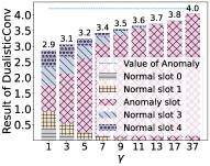
(a) An example for peak convolution.

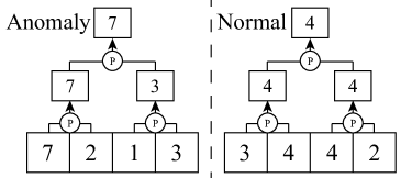
(b) Dualistic convolution in the frequency domain.

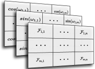
(c) The three channels of frequency representation.

Figure 3: (a) The figure shows the contributions of different time slots in peak convolution result in a convolution window when specifying different $\gamma$. As $\gamma$ grows, the contribution of deviations increases significantly. (b) The dualistic convolution applying to the frequency domain actually picks the prominent deviation in each compression step. (c) The figure shows the three channels of frequency representation in the frequency characterization module. The first channel is the result of Fourier transformation, the second is corresponding $sin$ Fourier bases and the third is corresponding $cos$ Fourier bases.

II-C Pattern Extraction

The most challenging problem in tackling diverse normal patterns with a unified model is that an anomaly for one normal pattern can be normal for another. To overcome this issue, we propose a pattern extraction mechanism to detect anomalies by the correlation between the data sample and its service normal pattern, instead of the data sample itself, which allows us to handle various normal patterns and reduce computational overhead by capitalizing on the sparsity inherent in the frequency domain. Our pattern extraction mechanism comprises three key components: a context-aware discrete Fourier transformation (DFT) module, a frequency characterization module, and a context-aware inverse discrete Fourier transformation (IDFT) module. In the preprocessing stage, we analyze each service in the frequency domain and identify a normal pattern subspace containing most of the normalities as the service normal pattern subspace by establishing a compact set of dominant Fourier bases for each normal pattern. During both the training and testing phases, we employ the context-aware DFT module to project time series data to its service normal pattern subspace by approximating it with a linear combination of the bases within the relevant normal pattern subspace. This procedure effectively compresses the spectral volume and minimizes computational demands. Subsequently, the frequency characterization module is used to create a tailored frequency representation for the time series data from its projection. After undergoing reconstruction through a dualistic convolution-based auto-encoder, the spectrum is transformed back into time series data using the context-aware IDFT. Furthermore, we theoretically prove that utilizing only the dominant bases for each normal pattern yields superior performance in distinguishing anomalies from normal patterns compared to using the complete spectrum. This is further supported by experimental evidence in Section III-D.

Context-aware DFT and context-aware IDFT. It is assumed that each service or server exhibits its unique normal pattern. Consequently, during the preprocessing stage, we process the training dataset in the frequency domain and count the occurrences of each Fourier base as the first $k$ strongest signals across all sliding windows. Subsequently, we select the top $k$ bases with the highest incidence to serve as Fourier bases for their service normal patterns subspace. In both the training and testing phases, the context-aware DFT transforms the time series data exclusively using the bases from the corresponding normal pattern subspace through the DFT process. Likewise, the context-aware IDFT processes the spectrum using only the corresponding bases through the IDFT. Furthermore, we conduct a theoretical comparison of the reconstruction error between anomalies and normal patterns, demonstrating that the context-aware DFT can significantly widen the gap in reconstruction errors between anomalies and normal patterns.

Definition 2 (Spectrum). Given a DFT spectrum of a normal pattern $\mathcal{A}_{N}(\omega_{0})>\dots>\mathcal{A}_{N}(\omega_{n})$, where $\mathcal{A}_{N}(\omega_{i})$ is the amplitude of the signal and $\omega_{i}$ is its corresponding frequency, we compute normalized value of them as follows: $q_{N}(\omega_{i})=\frac{\mathcal{A}_{N}(\omega_{i})}{\sum_{i=1}^{n}\mathcal{A}_{N}(\omega_{i})}$. The spectrum of anomalies is denoted by $\mathcal{A}_{A}(\omega_{0}),\dots,\mathcal{A}_{A}(\omega_{n})$, where $\omega_{i}$ is exactly the $\omega_{i}$ in spectrum of normal pattern. Similarly, the spectrum of anomalies is normalized and denoted by $q_{A}(\omega_{i})$. The normalized spectrum for normalities and anomalies obtained by context-aware DFT are denoted by $\bar{q}_{N}(\omega_{i})$ and $\bar{q}_{A}(\omega_{i})$ respectively.

Definition 3 (Reconstruction error). The reconstruction error of context-aware DFT is defined as the KL divergence between the spectrum obtained by context-aware DFT and the original spectrum, i.e. $\operatorname{KL}(\bar{q}|q)$.

Assumption 1. The anomalies manifest themselves by adding a shift variable to the spectrum of normalities, whose expectation is greater than 0, i.e. $\mathcal{A}_{A}(\omega_{i})=\mathcal{A}_{N}(\omega_{i})+\Delta\mathcal{A}_{i}$, where $\forall i,\Delta\mathcal{A}_{i}$ are independent identically distributed and follow an unknown distribution with expectation $\Delta A$, $\Delta A>0$. It is reasonable to assume the expectation of shift variable is bigger than 0 since it is reported that the anomalies have stronger signals than normalities [14], which implies higher amplitude expectations of anomalies. Moreover, we statistically collect the expectation of anomalies and normalities across three real-world datasets and verify this point, as shown in Tab.III.

TABLE III: The expectation of amplitudes for anomalies and normalities on different datasets.

	SMD	J-D1	J-D2
Anomaly	0.36	0.74	0.81
Normality	0.23	0.72	0.77

Theorem 2. The gap of reconstruction error between the anomaly and normality is $\log\frac{\sum_{i=1}^{k}q_{N}(\omega_{i})}{\sum_{i=1}^{k}q_{A}(\omega_{i})}$.

Proof. Using the normality as an example, we derive the expression for its reconstruction error. The expression for an anomaly can be derived in a similar manner. To begin, we can represent $\bar{q}_{N}$ as shown in Eq. 8. Subsequently, the reconstruction error for it is obtained in Eq. 9. As a result, the gap in the reconstruction error between anomalies and normal patterns is given by $\operatorname{KL}(\bar{q}_{A}|q_{A})-\operatorname{KL}(\bar{q}_{N}|q_{N})=\log\frac{\sum_{i=1}^{k}q_{N}(\omega_{i})}{\sum_{i=1}^{k}q_{A}(\omega_{i})}$.

$$\bar{q}_{N}(\omega_{i})=\left\{\begin{matrix}\frac{q_{N}(\omega_{i})}{\sum_{i=1}^{k}q_{N}(\omega_{i})}&,i\leq k\\ 0&,i>k\end{matrix}\right.$$ (8)

$$\begin{split}\operatorname{KL}(\bar{q}_{N}|q_{N})&=\sum_{j=1}^{k}\frac{q_{N}(\omega_{j})}{\sum_{i=1}^{k}q_{N}(\omega_{i})}\log\frac{1}{\sum_{t=1}^{k}q_{N}(\omega_{t})}\\ &=-\frac{\sum_{j=1}^{k}q_{N}(\omega_{j})}{\sum_{t=1}^{k}q_{N}(\omega_{t})}\log\sum_{i=1}^{k}q_{N}(\omega_{i})\\ &=-\log\sum_{i=1}^{k}q_{N}(\omega_{i})\end{split}$$ (9)

Intuitively, the gap is greater than 0 because the numerator of it, $\sum_{i=1}^{k}q_{N}(\omega_{i})$, represents the first $k$ strongest signals, while the denominator, $\sum_{i=1}^{k}q_{A}(\omega_{i})$, is not guaranteed to have a similar characteristic. We have conducted a further analysis of the condition for achieving a smaller reconstruction error for normal patterns in Corollary 1.

Corollary 1. When $\sum_{i=1}^{k}q_{N}(\omega_{i})>\frac{k}{n}$, the reconstruction error of normality is smaller than that of anomaly.

Proof. According to assumption 1, the $q_{A}(\omega_{i})$ can be transformed into $\frac{q_{N}(\omega_{i})S+{\Delta\mathcal{A}_{i}}}{S+{\sum_{i=1}^{n}\Delta\mathcal{A}_{i}}}$, where $S=\sum_{i=1}^{n}\mathcal{A}_{N}(\omega_{i})$. Thus, the gap of reconstruction error between anomaly and normality can be transformed to $\log\frac{S+n\Delta A}{S+k\Delta A(\sum_{j=1}^{k}q_{N}(\omega_{j}))^{-1}}$ according to the Law of Large Numbers [24]. When $\sum_{i=1}^{k}q_{N}(\omega_{i})>\frac{k}{n}$, we can obtain $S+n\Delta A>S+k\Delta A(\sum_{j=1}^{k}q_{N}(\omega_{j}))^{-1}$. As a result, the gap of reconstruction error is bigger than 0.

It is worth noticing that when using trivial DFT and completed spectrum, $k$ is set to $n$ and the reconstruction error gap of anomaly and normality becomes zero, considering that $q_{A}$ and $q_{N}$ are normalized values. In contrast, examining the condition in Corollary 1, it becomes evident that there must be a value of $k$ less than $n$ that yields a reconstruction error gap greater than 0. Thus, compared with using the full spectrum, only using a subset of them widens the reconstruction error gap between the normalities and anomalies. This confirms that anomalies are easier to distinguish when employing the context-aware DFT with a reduced set of bases compared to the standard DFT.

Frequency characterization. The frequency characterization module concatenates the result of context-aware DFT and explicit marked trigonometric bases, as shown in Fig.3(c), where $\mathcal{F}_{i,j}$ denotes the Fourier result of $j^{th}$ base for $i^{th}$ feature dimension, $\omega_{i,j}$ denotes the frequency of $j^{th}$ base for $i^{th}$ feature dimension. Afterwards, we use a three-channel convolution to manipulate the concatenated tensors and obtain the frequency representation.

III Experiment

We conduct extensive experiments on four real-world anomaly detection datasets and obtain the following conclusions:

• When detecting anomalies for multiple services with kinds of normal patterns by a unified model, MACE achieves better performance compared with the state-of-the-art methods.

• MACE achieves comparable performance compared with the state-of-the-art methods when the state-of-the-art methods are trained separately for each service and MACE uses a unified model for all the services.

• MACE shows good transferability on unseen datasets.

• MACE consumes obviously less time and memory overhead than the state-of-the-art methods.

• Every module in MACE contributes to its performance.

III-A Experiment Setup

The datasets used in this paper contain several subsets, which represent data for different services, servers and detecting sensors. It is assumed that different subsets have different normal patterns. We divide every ten subsets in a dataset as a group. For each group, we train a unified model to detect the anomaly in it.

Hyperparameter. The important hyperparameters of MACE are shown in Tab.IV, where $m$ denotes the number of basis in a subset, $\gamma_{f}$ denotes $\gamma$ for the dualistic convolution in the frequency domain, $\gamma_{t}$ denotes the one in the time domain, $\sigma_{f}$ denotes the scaling factor of dualistic convolution in the frequency domain and $\sigma_{t}$ denotes the one in the time domain.

TABLE IV: Hyperparameters of MACE.

Hyperparameter	Value	Hyperparameter	Value
$m$	20	$\gamma_{f}$ in SMD	7
$\gamma_{t}$ in SMD	11	$\gamma_{f}$ in J-D1	11
$\gamma_{t}$ in J-D1	11	$\gamma_{f}$ in J-D2	13
$\gamma_{t}$ in J-D2	13	$\gamma_{f}$ in SMAP	13
$\gamma_{t}$ in SMAP	13	$\sigma_{f}$ in SMD	5
$\sigma_{t}$ in SMD	5	$\sigma_{f}$ in J-D1	5
$\sigma_{t}$ in J-D1	5	$\sigma_{f}$ in J-D2	5
$\sigma_{t}$ in J-D2	5	$\sigma_{f}$ in SMAP	5
$\sigma_{t}$ in SMAP	7	kernel length	5
window size	40	learning rate	0.001

Baselines. We conducted a comprehensive comparison of MACE with several state-of-the-art methods, including DCdetector [25], AnomalyTransformer [26], DVGCRN [27], JumpStarter [14], OmniAnomaly [17], and MSCRED [18]. To assess its diverse pattern generalization capabilities, we introduced two additional methods: TranAD, a meta-learning-based approach [19], and ProS, a transfer-learning-based method [28]. Furthermore, to evaluate its computational efficiency, we compared MACE with the classical anomaly detection method VAE [29]. Due to space constraints, some figures represent methods using the first two letters of their names as a shorthand.

• DCdetector (DC) [25]: DCdetector is a latest cutting-edge anomaly detection method. It employs a unique dual attention asymmetric design to establish a permuted environment and leverages pure contrastive loss to guide the learning process. This enables the model to learn a permutation-invariant representation with superior discrimination abilities.

• AnomalyTransformer (An) [26]: Anomaly Transformer stands out as one of the most cutting-edge methods, harnessing the formidable capabilities of transformers to model point-wise representation and pair-wise associations through an innovative anomaly-attention mechanism.

• DVGCRN (DV) [27]: DVGCRN stands out as another cutting-edge anomaly detection method, effectively modeling fine-grained spatial and temporal correlations in multivariate time series. It achieves a precise posterior approximation of latent variables, contributing to a robust representation of multivariate time series data.

• JumpStarter (Ju) [14]: JumpStarter stands out as a cutting-edge anomaly detection method, equipped with a shape-based clustering and an outlier-resistant sampling algorithm. This combination ensures a rapid initialization and high F1 score performance.

• OmniAnomaly (Om) [17]: OmniAnomaly is a widely acknowledged anomaly detection method, employing a stochastic variable connection and planar normalizing flow to robustly capture the representation of normal multivariate time series data.

• MSCRED (MS) [18]: MSCRED is a highly acclaimed method known for its ability to detect anomalies across various scales and pinpoint root causes through the utilization of multi-scale signature matrices.

• TranAD (Tr) [19]: TranAD, a meta-learning-based anomaly detection method, represents one of the latest cutting-edge approaches. It excels in learning a robust initialization for anomaly detection models, demonstrating excellent generalization across diverse normal patterns.

• ProS (Pr) [28]: ProS introduces a zero-shot methodology, capable of inferring in the target domains without the need for re-training. This is achieved through the introduction of latent domain vectors, serving as latent representations of the domains.

• VAE (VA) [29]: VAE, a widely recognized and classical anomaly detection method, serves as a foundational framework for numerous state-of-the-art approaches. It introduces low computational and memory overhead, contributing to its popularity.

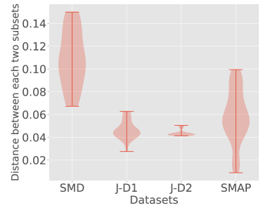
(a) KL divergence distance distribution between kernel density estimation distributions of pairwise subsets

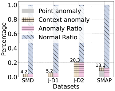
(b) The ratios of point anomaly, context anomaly and normal patterns in each dataset

Figure 4: (a) We first use kernel density estimation to estimate the distribution of each subset. Subsequently, we compute KL divergence between each pair of subsets in a training group. The figure shows the distribution of the KL divergences of different datasets. (b) The figure shows the point anomaly, context anomaly and normal pattern ratios in each dataset.

Datasets. We utilized a selection of datasets, including the widely-recognized Server Machine Dataset (SMD), two cloud service monitoring logs from a top global Internet company (J-D1 and J-D2), and the well-established anomaly detection benchmark, Soil Moisture Active Passive (SMAP). As shown in Fig.4, the normal patterns of SMD are the most diverse, while the normal patterns of J-D2 are the most similar. Moreover, SMAP has most point anomalies, while the anomalies in other datasets are lasting.

• Server Machine Dataset (SMD) [17]: SMD spans a 5-week period and originates from a major Internet company, incorporating data from 28 distinct machines. Each machine’s log data, a subset of SMD, is equally divided into training and testing sets. The anomaly ratio in SMD is 4.16%.

• Datasets provided by Jumpstarter (J-D1 and J-D2) [14]: J-D1 and J-D2 are two datasets gathered from a top global Internet company. Each dataset includes logs of 19 metrics from 30 services, with each service’s log data forming a subset in J-D1 and J-D2. The anomaly ratios for J-D1 and J-D2 are 5.25% and 20.26%, respectively.

• Soil Moisture Active Passive (SMAP) [30]: SMAP comprises real spacecraft telemetry data and anomalies from the Soil Moisture Active Passive satellite, featuring an anomaly ratio of 13.13%.

TABLE V: The performance of MACE and baselines when detecting anomalies for multiple patterns by a unified model.

	SMD			J-D1			J-D2			SMAP
	Precision	Recall	F1	Precision	Recall	F1	Precision	Recall	F1	Precision	Recall	F1
DCdetector	0.680	0.672	0.669	0.709	0.583	0.626	0.956	0.897	0.923	0.594	0.613	0.597
AnomalyTransformer	0.439	0.947	0.562	0.519	0.945	0.639	0.824	0.981	0.891	0.610	0.947	0.699
DVGCRN	0.481	0.766	0.481	0.344	0.737	0.421	0.695	0.867	0.742	0.475	0.979	0.549
OmniAnomaly	0.674	0.829	0.713	0.957	0.868	0.899	0.948	0.932	0.938	0.789	0.984	0.819
MSCRED	0.444	0.562	0.407	0.880	0.806	0.819	0.927	0.944	0.932	0.838	1.000	0.884
TranAD	0.617	0.616	0.471	0.198	0.631	0.258	0.729	0.952	0.797	0.275	0.577	0.291
ProS	0.153	0.785	0.214	0.505	0.731	0.534	0.796	0.861	0.805	0.412	0.973	0.468
VAE	0.221	0.689	0.246	0.377	0.796	0.425	0.566	0.909	0.665	0.470	0.983	0.557
MACE	0.964	0.870	0.910	0.893	0.984	0.934	0.938	0.989	0.961	0.958	1.000	0.977

Metrics. We use three of the most widely-used metrics to evaluate the performance of MACE and baseline methods as many prominent anomaly detection papers [27, 25, 19, 14] do: the precision, recall and F1 score. The definitions of these metrics are given in Eq.10, where $TP$, $FP$ and $FN$ denote true positive, false positive and false negative respectively.

$$\begin{split}\operatorname{Precision}&=\frac{TP}{TP+FP}\\ \operatorname{Recall}&=\frac{TP}{FN+TP}\\ \operatorname{F1}=2*&\frac{\operatorname{Precision}*\operatorname{Recall}}{\operatorname{Precision}+\operatorname{Recall}}\end{split}$$ (10)

III-B Prediction Accuracy

In this subsection, we conduct extensive experiments to validate that MACE consistently achieves the best F1 score compared to baselines when distinguishing anomalies from different normal patterns with a unified model. Furthermore, in comparison to baselines that tailor a unique model for each subset, MACE demonstrates competitive performance with a unified model. Additionally, owing to the memory-guided pattern extraction method, MACE exhibits commendable performance on previously unseen normal patterns.

Adaptability to Multiple Normal Patterns. We assume that various subsets in the four datasets contain distinct normal patterns, representing logs for different servers (SMD), services (J-D1 and J-D2), and data for different detector channels (SMAP). During the training stage, every ten subsets in a dataset are grouped together and utilized to train a unified model. In the testing stage, the trained model is applied to detect anomalies in each corresponding testing subset independently. The average metrics for different subsets are presented in Table V, where the best results are highlighted in bold, and the second-best results are underlined. Since JumpStarter is a signal-based method, multiple normal pattern training is not applicable to it, and thus, JumpStarter is excluded from this analysis. As indicated in Table V, despite occasional deviations, MACE achieves the best performance when detecting multiple normal patterns with a unified model. Moreover, MACE consistently achieves the best F1 score when compared with all the baselines across the four datasets. Furthermore, the improvement is substantial: MACE increases the F1 score by an average of 8.7% compared to the best baseline performance. As illustrated in Fig. 4(a), the subsets in SMD exhibit significant differences from each other, where MACE shows a distinct advantage. Intuitively, since the normal patterns in J-D2 are very similar to each other, most methods perform well on this dataset and the advantage of MACE is not as obvious as the one on the former dataset. Additionally, MACE attains a high F1 score on SMAP. Considering that most anomalies in SMAP are point anomalies, this result verifies the effectiveness of dualistic convolution in the time domain, which extends the detection capabilities for short-term anomalies and makes them easier to identify.

TABLE VI: Performance of MACE detecting anomaly with a unified model for different patterns, compared with the ones of baselines that customize a unique model for each normal pattern.

	SMD			J-D1			J-D2			SMAP
	Precision	Recall	F1	Precision	Recall	F1	Precision	Recall	F1	Precision	Recall	F1
DCdetector	0.836	0.911	0.872	0.766	0.744	0.748	0.956	0.880	0.913	0.956	0.989	0.970
AnomalyTransformer	0.894	0.955	0.923	0.520	0.918	0.645	0.818	0.998	0.896	0.941	0.994	0.967
DVGCRN	0.950	0.883	0.915	0.395	0.806	0.479	0.711	0.852	0.723	0.916	0.920	0.914
JumpStarter	0.904	0.943	0.923	0.921	0.945	0.933	0.941	0.996	0.968	0.471	0.995	0.526
OmniAnomaly	0.695	0.877	0.728	0.891	0.940	0.905	0.945	0.974	0.958	0.713	0.963	0.744
MSCRED	0.746	0.744	0.716	0.975	0.830	0.889	0.949	0.969	0.958	0.872	1.000	0.923
TranAD	0.926	0.997	0.961	0.251	0.918	0.349	0.754	0.965	0.817	0.804	1.000	0.892
ProS	0.146	0.822	0.206	0.422	0.767	0.506	0.763	0.921	0.821	0.447	0.973	0.509
VAE	0.286	0.585	0.255	0.334	0.866	0.385	0.702	0.890	0.763	0.579	0.973	0.648
MACE	0.964	0.870	0.910	0.893	0.984	0.934	0.938	0.989	0.961	0.958	1.000	0.977

TABLE VII: The performance of MACE and baselines for unseen normal patterns.

	SMD			J-D1			J-D2			SMAP
	Precision	Recall	F1	Precision	Recall	F1	Precision	Recall	F1	Precision	Recall	F1
DCdetector	0.681	0.685	0.681	0.798	0.771	0.781	0.948	0.857	0.891	0.700	0.760	0.724
AnomalyTransformer	0.490	0.916	0.622	0.555	0.948	0.667	0.838	0.981	0.899	0.586	1.000	0.678
DVGCRN	0.125	0.798	0.173	0.388	0.894	0.478	0.619	0.893	0.664	0.444	1.000	0.525
OmniAnomaly	0.686	0.780	0.701	0.976	0.824	0.880	0.932	0.953	0.941	0.735	0.986	0.794
MSCRED	0.418	0.593	0.409	0.828	0.818	0.806	0.931	0.952	0.939	0.839	1.000	0.896
TranAD	0.255	0.643	0.265	0.127	0.546	0.198	0.516	0.659	0.546	0.205	1.000	0.302
ProS	0.154	0.808	0.215	0.475	0.770	0.564	0.789	0.933	0.855	0.412	0.979	0.469
VAE	0.193	0.789	0.270	0.339	0.875	0.386	0.661	0.884	0.721	0.433	0.979	0.500
MACE	0.915	0.835	0.863	0.972	0.829	0.885	0.963	0.968	0.964	0.954	0.996	0.973

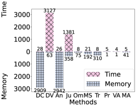
(a) Time (s) and memory overhead (*10kB).

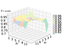
(b) The impact of $\gamma_{t}$ and $\gamma_{f}$ on MACE performance.

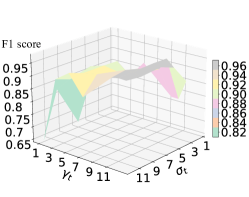
(c) The impact of $\gamma_{t}$ and $\sigma_{t}$ on MACE performance.

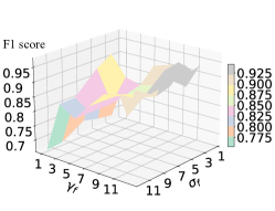
(d) The impact of $\gamma_{f}$ and $\sigma_{f}$ on MACE performance.

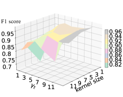
(e) The impact of kernel size and $\gamma_{t}$ on MACE performance.

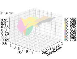
(f) The impact of number of basis in a subset and $\gamma_{f}$ on MACE performance.

Figure 5: Due to the space limitation, we use the first two letters in method names as a shorthand. $\gamma_{t}$ and $\gamma_{f}$ represent the powers in dualistic convolution for the time domain and frequency domain respectively. $\sigma_{t}$ and $\sigma_{f}$ represent the scaling factors in dualistic convolution for the time domain and frequency domain respectively. (a) The time and memory overhead of MACE and baselines. (b) The F1 score of MACE for grid search of $\gamma_{t}$ and $\gamma_{f}$. (c) The F1 score of MACE for grid search of $\gamma_{t}$ and $\sigma_{t}$. (d) The F1 score of MACE for grid search of $\gamma_{f}$ and $\sigma_{f}$. (e) The F1 score of MACE for grid search of dualistic convolution kernel size in the time domain and $\gamma_{t}$. (f) The F1 score of MACE for grid search of the number of bases in a subset and $\gamma_{f}$.

Competitive Performance Compared to Customizing a Unique Model. In this experiment, MACE employs a unified model for every ten different normal patterns, while baselines customize a unique model for each normal pattern. As depicted in Table VI, MACE achieves comparable performance with the strongest state-of-the-art methods. It is noteworthy that MACE captures ten different patterns simultaneously with a single model, a factor that generally hinders model performance [15], while baselines customize a unique model for each normal pattern. The negative impact of multiple normal patterns is further evident when comparing Table V and Table VI: when normal patterns are diverse (e.g., in SMD), the baselines in Table VI, where they tailor a unique model for each normal pattern, exhibit big strength compared to their performance in Table V, where they learn a unified model for multiple normal patterns. In contrast, when normal patterns are similar (e.g., in J-D2), the baseline performance gaps between Tables V and VI are narrow. From this comparison, it can be concluded that the diversity of normal patterns hinders model performance when using a unified model for multiple patterns. Thus, it is tolerable for MACE to exhibit a somewhat lower F1 score on SMD, considering that the normal patterns of SMD are the most diverse among the four datasets.

MACE Performance on Unseen Normal Patterns. As mentioned earlier, different subsets are assumed to represent different normal patterns, and every ten subsets in a dataset are divided into a group. MACE and all the baselines are trained on one group and tested on another. The results are presented in Table VII, where the best performances are bolded, and the second-best performances are underlined. Since JumpStarter is a signal-based method, training on one group while testing on another is not applicable to it, and thus, it is not included in the table. As shown in Table VII, MACE consistently achieves the highest F1 score on the four datasets. The performance of MACE when the normal patterns are diverse, such as in SMD, is lower than when the normal patterns are similar, such as in J-D2. When the distance between different normal patterns is small, MACE can achieve similar F1 scores to those when MACE is trained and tested on the same group (i.e., the performance on J-D2 and SMAP).

TABLE VIII: The performances of MACE when removing different modules

Remove module	SMD			J-D1			J-D2			SMAP
	Precision	Recall	F1	Precision	Recall	F1	Precision	Recall	F1	Precision	Recall	F1
Context-aware DFT & IDFT	0.762	0.813	0.762	0.624	0.887	0.689	0.958	0.953	0.953	0.775	1.000	0.831
Dualistic Convolution (F)	0.187	0.943	0.184	0.855	0.854	0.820	0.857	0.933	0.886	0.681	0.990	0.713
Dualistic Convolution (T)	0.046	0.842	0.084	0.089	0.946	0.152	0.208	0.440	0.250	0.682	0.989	0.720
Frequency Characterization	0.894	0.860	0.868	0.838	0.940	0.857	0.970	0.980	0.975	0.944	1.000	0.967
Pattern extraction	0.714	0.702	0.696	0.667	0.914	0.740	0.957	0.953	0.954	0.770	0.970	0.797
MACE	0.964	0.870	0.910	0.893	0.984	0.934	0.938	0.989	0.961	0.958	1.000	0.977

III-C Time and Memory Overhead

We evaluated both time and memory overhead on a server equipped with a configuration comprising 32 Intel(R) Xeon(R) CPU E5-2620 @ 2.10GHz CPUs and 2 K80 GPUs. For neural network-based methods, we employed a profiling tool to assess their memory overhead. In the case of JumpStarter, a signal-based method, we record its maximum memory consumption during the inference process. The time overhead was calculated based on the training time of each method on a subset group of the SMD dataset. The results, depicted in Fig. 5(a), reveal that MACE’s time overhead is competitive with some very simple methods, such as VAE and ProS based on VAE, while MACE’s F1 scores significantly surpass the ones of them across all four datasets. Regarding memory overhead, MACE’s value is higher than that of a two-layer VAE and ProS based on a two-layer VAE. However, MACE’s memory overhead is considerably lower than that of other deep neural networks. These findings underscore MACE’s efficiency in terms of both time and memory usage, positioning it favorably among deep neural-network-based methods and showcasing superior performance in terms of anomaly detection as evidenced by its higher F1 scores across diverse datasets.

III-D Ablation Study

We conducted experiments to assess the effectiveness of individual modules within MACE by removing them individually. When the context-aware Discrete Fourier Transform (DFT) and Inverse DFT (IDFT) modules were removed, they were replaced with conventional DFT and IDFT. The results are displayed in Table VIII, where ”Dualistic Convolution (F)” and ”Dualistic Convolution (T)” correspond to dualistic convolution in the frequency and time domains, respectively.

As depicted in Table VIII, the complete MACE model exhibits considerable superiority over its variants. It is worth noting that when context-aware DFT and IDFT are substituted with vanilla counterparts, MACE’s performance takes a sharp nosedive. The computational and memory overhead of vanilla DFT and IDFT increases because they introduce more Fourier bases, yet the performance deteriorates. This observation aligns with our earlier theoretical analysis.

Moreover, this experiment underscores the effectiveness of the diverse normal pattern adaptability facilitated by the pattern extraction mechanism. This module significantly enhances performance on SMD, characterized by diverse normal patterns, while showing marginal improvement on J-D2, where the normal patterns are similar. Similarly, the frequency characterization module makes a substantial contribution on SMD but is of limited use on J-D2, given its multi-pattern extraction nature. In summary, the module-by-module evaluation reaffirms the crucial role played by various components in MACE and their impact on anomaly detection performance across different datasets.

III-E The impact of hyperparameter

We employed grid search to investigate the influence of critical hyperparameters on the performance of MACE. Fig.5(b)-Fig.5(f) present the F1 scores corresponding to different combinations of pairwise hyperparameters. The search ranges for $\gamma$ in the time domain and frequency domain, $\sigma$ in the time domain and frequency domain, kernel size, and the number of Fourier bases in Context-aware DFT and IDFT were set to {1, 3, 5, 7, 11, 12, 13}, {3, 5, 7, 10, 12}, {3, 5, 7, 11, 13}, and {5, 10, 15, 20, 25, 30} respectively.

Impact of $\gamma_{t}$ and $\gamma_{f}$: When $\gamma_{t}$ and $\gamma_{f}$ are set to 1, dualistic convolution degenerates into a trivial convolution, essentially nullifying its contribution. Consequently, MACE’s performances with $\gamma_{t}$ and $\gamma_{f}$ set to 1 are unsatisfied. In general, the performance of MACE improves as $\gamma_{t}$ and $\gamma_{f}$ increase, as depicted in Fig.5(c) and Fig.5(d). However, it’s important to note that $\gamma$ cannot grow infinitely, as excessively large $\gamma$ values can lead to gradient explosions. Thus, setting $\gamma$ within the search space mentioned above is a safe approach.

Impact of $\sigma_{t}$ and $\sigma_{f}$: These scaling factors are introduced to mitigate gradient explosions. As demonstrated in Fig.5(c)-Fig.5(d), MACE’s performance remains stable across various values of $\sigma$.

Impact of dualistic convolution kernel size in the time domain: Intuitively, the performance of MACE initially improves and then declines as the kernel size increases, as shown in Figure 5(e). That is because when the kernel size increases from a small value, it makes anomalies more prominent and easier to detect. However, when the kernel size becomes excessively large, the dualistic convolution in the time domain distorts the original time series and detrimentally affects model performance.

Impact of the number of Fourier bases in Context-aware DFT and IDFT: The performance of MACE generally follows an increasing-then-decreasing pattern as the number of bases grows. As analyzed theoretically in Section.II-C, when the number of bases increases from a small value, both the reconstruction of normal patterns and anomalies improve, but the enhancement in normality reconstruction is more pronounced. However, when the number of bases becomes relatively large, the improvement in normality reconstruction becomes marginal, while the effect on anomaly reconstruction becomes significant. Therefore, the performance initially increases and then declines with the growth of the number of bases.

IV Related Work

Anomaly detection is a crucial task that focuses on identifying outliers within time series data and has been the subject of extensive research. The existing body of work can be broadly categorized into three main groups: classical machine learning and statistical methods, signal processing-based methods, and deep learning-based methods. In the following, we provide a brief overview of each category and a review of multi-task learning since multiple normal pattern learning is highly correlated to the aim of this work. Moreover, we also review the anomaly detection methods used in the cloud center.

IV-A Anomaly detection

The classical machine learning and statistical methods. Conventional statistical and machine learning methods, as highlighted in earlier works [31, 32, 33], operate without the need for extensive training data and remain unaffected by the challenge of diverse normal patterns. Furthermore, they typically incur little computational overhead. Despite these advantages, these approaches are contingent upon certain assumptions and, in real-world applications, exhibit constrained robustness [14].

The signal-processing-based methods. Signal processing-based methods leverage the advantages of fine-grained parallelism and the sparsity inherent in the frequency domain. Despite these advantages, they encounter difficulties in simultaneously capturing both global and subtle features while maintaining manageable computational overhead. For instance, the Fourier transform [34] excels at capturing global information but struggles with subtle local features. In contrast, context-aware Discrete Fourier Transform (DFT) and context-aware Inverse DFT (IDFT) select Fourier bases based on a given normal pattern and integrate with dualistic convolution mechanism, enhancing the capacity to extract subtle features. The theoretical evidence supports that this approach widens the reconstruction error gap between anomalies and normal patterns. Unlike the Fourier transform, wavelet analysis [35] can effectively capture local patterns but is highly time-consuming. Classical signal processing techniques, such as Principal Component Analysis (PCA) and Kalman Filtering [36], lack competitiveness in detecting anomalies in variational time series. JumpStarter [14], a recent state-of-the-art method in this category, suffers from significant inference time overhead and struggles to handle heavy traffic loads in real time.

The deep learning-based methods. Deep learning-based methods prove to be particularly effective for variable time series [19]. These methods can be broadly categorized into prediction-based approaches [30, 37], reconstruction-based methods [26, 27], and classifier-based methods [38, 39, 40]. Prediction-based methods, such as LSTM-NDT [30] and DAGMM [37], incorporate recurrent networks, which are non-parallelizable and inefficient. Similarly, reconstruction-based methods like Donut [11] and OmniAnomaly [17] also rely on recurrent neural networks. Recent advancements, exemplified by USAD [41] and GDN [42], replace recurrent neural networks with attention-based architectures to expedite the training process. However, these methods face challenges in effectively capturing long-term dependencies due to the removal of recurrent networks and the use of small input windows [19]. In contrast to these approaches, anomaly detection in the frequency domain eliminates temporal dependencies without sacrificing global information. Consequently, there is no need for recurrent neural networks, yet the model can still effectively capture long-term features. The most recent works leverage the power of transformers, exemplified by AnomalyTransformer [26] and TranAD [19], enabling fine-grained parallelism. However, these methods encounter challenges in handling diverse normal patterns with a unified model.

IV-B Multi-task learning

Multitask Learning (MTL) is a machine learning paradigm where a model is trained to perform multiple related tasks simultaneously. Instead of training separate models for each task, MTL allows for the sharing of certain model parameters, enabling the model to learn common representations across tasks. The research in this domain can be divided into two categories: the hard-sharing methods and the soft-sharing methods. The hard-sharing methods share common low-level hidden layers, while the soft-sharing methods communicate general knowledge between several models by adding regularization on neural network parameters [43] or inserting connection across networks [44, 45]. However, either the soft-sharing methods or the hard-sharing methods need to maintain tailored neural network layers for each task, which is still expensive for millions of services.

IV-C The anomaly detection methods for a cloud system.

Anomaly detection methods within cloud systems serve the purpose of identifying intrusions, addressing failures, monitoring performance, and analyzing the root causes of issues across servers, services, and networks [46]. Intrusion detection primarily focuses on safeguarding against network intrusions, including DDoS/DoS, Botnet, Malware, and Fraud storm attacks. Performance monitoring aims to detect sudden performance degradation, which typically leads to a decrease in system efficiency [47]. Failure detection seeks to distinguish service failures, container failures, and hardware failures [46]. Additionally, certain anomaly detection methods offer techniques for root cause localization, such as comparing the reconstruction error of each feature [17], computing derivatives for each feature [48], introducing perturbations to each feature [49], and employing game theory for localization [50], among other approaches.

V Conclusion

In this work, we address the challenges of detecting anomalies from diverse normal patterns with a unified and efficient model as well as improve the short-term anomaly sensitivity by proposing MACE. MACE exhibits three key characteristics: (i) a pattern extraction mechanism allowing the model to detect anomalies by the correlation between the data sample and its service normal pattern and adapt to the diverse nature of normal patterns; (ii) a dualistic convolution mechanism that amplifies anomalies in the time domain and hinders the reconstruction in the frequency domain; (iii) the utilization of the inherent sparsity and parallelism of the frequency domain to enhance model efficiency. We substantiate our approach through both mathematical analysis and extensive experiments, demonstrating that selecting a subset of Fourier bases based on normal patterns yields superior performance compared to utilizing the complete spectrum. Comprehensive experiments confirm MACE’s proficiency in effectively handling diverse normal patterns, showcasing optimal performance with high efficiency when benchmarked against state-of-the-art methods.

References

- [1] G. Zhang, C. Li, K. Zhou, L. Liu, C. Zhang, W. Chen, H. Fang, B. Cheng, J. Yang, and J. Xing, “Dbcatcher: A cloud database online anomaly detection system based on indicator correlation,” in 2023 IEEE 39th International Conference on Data Engineering (ICDE). IEEE, 2023, pp. 1126–1139.
- [2] S. Ramaswamy, R. Rastogi, and K. Shim, “Efficient algorithms for mining outliers from large data sets,” in Proceedings of the 2000 ACM SIGMOD international conference on Management of data, 2000, pp. 427–438.
- [3] X. Wang, J. Lin, N. Patel, and M. Braun, “Exact variable-length anomaly detection algorithm for univariate and multivariate time series,” Data Mining and Knowledge Discovery, vol. 32, pp. 1806–1844, 2018.
- [4] V. Gómez-Verdejo, J. Arenas-García, M. Lazaro-Gredilla, and Á. Navia-Vazquez, “Adaptive one-class support vector machine,” IEEE Transactions on Signal Processing, vol. 59, no. 6, pp. 2975–2981, 2011.
- [5] P. Boniol, M. Linardi, F. Roncallo, T. Palpanas, M. Meftah, and E. Remy, “Unsupervised and scalable subsequence anomaly detection in large data series,” The VLDB Journal, pp. 1–23, 2021.
- [6] A. Siffer, P.-A. Fouque, A. Termier, and C. Largouet, “Anomaly detection in streams with extreme value theory,” in Proceedings of the 23rd ACM SIGKDD international conference on knowledge discovery and data mining, 2017, pp. 1067–1075.
- [7] S. Subramaniam, T. Palpanas, D. Papadopoulos, V. Kalogeraki, and D. Gunopulos, “Online outlier detection in sensor data using non-parametric models,” in Proceedings of the 32nd international conference on Very large data bases, 2006, pp. 187–198.
- [8] H. Ren, B. Xu, Y. Wang, C. Yi, C. Huang, X. Kou, T. Xing, M. Yang, J. Tong, and Q. Zhang, “Time-series anomaly detection service at microsoft,” in Proceedings of the 25th ACM SIGKDD international conference on knowledge discovery & data mining, 2019, pp. 3009–3017.
- [9] M. Thill, W. Konen, and T. Bäck, “Online adaptable time series anomaly detection with discrete wavelet transforms and multivariate gaussian distributions,” Archives of Data Science, Series A (Online First), vol. 5, no. 1, p. 17, 2018.
- [10] M. Thill, W. Konen, and T. Back, “Time series anomaly detection with discrete wavelet transforms and maximum likelihood estimation,” in Intern. Conference on Time Series (ITISE), vol. 2, 2017, pp. 11–23.
- [11] H. Xu, W. Chen, N. Zhao, Z. Li, J. Bu, Z. Li, Y. Liu, Y. Zhao, D. Pei, Y. Feng et al., “Unsupervised anomaly detection via variational auto-encoder for seasonal kpis in web applications,” in Proceedings of the 2018 world wide web conference, 2018, pp. 187–196.
- [12] X. Chen, L. Deng, F. Huang, C. Zhang, Z. Zhang, Y. Zhao, and K. Zheng, “Daemon: Unsupervised anomaly detection and interpretation for multivariate time series,” in 2021 IEEE 37th International Conference on Data Engineering (ICDE). IEEE, 2021, pp. 2225–2230.
- [13] T. Kieu, B. Yang, C. Guo, R.-G. Cirstea, Y. Zhao, Y. Song, and C. S. Jensen, “Anomaly detection in time series with robust variational quasi-recurrent autoencoders,” in 2022 IEEE 38th International Conference on Data Engineering (ICDE). IEEE, 2022, pp. 1342–1354.
- [14] M. Ma, S. Zhang, J. Chen, J. Xu, H. Li, Y. Lin, X. Nie, B. Zhou, Y. Wang, and D. Pei, “Jump-Starting multivariate time series anomaly detection for online service systems,” in 2021 USENIX Annual Technical Conference (USENIX ATC 21), 2021, pp. 413–426.
- [15] H. Park, J. Noh, and B. Ham, “Learning memory-guided normality for anomaly detection,” in Proceedings of the IEEE/CVF conference on computer vision and pattern recognition, 2020, pp. 14 372–14 381.
- [16] J. Chung, K. Kastner, L. Dinh, K. Goel, A. C. Courville, and Y. Bengio, “A recurrent latent variable model for sequential data,” Advances in neural information processing systems, vol. 28, 2015.
- [17] Y. Su, Y. Zhao, C. Niu, R. Liu, W. Sun, and D. Pei, “Robust anomaly detection for multivariate time series through stochastic recurrent neural network,” in Proceedings of the 25th ACM SIGKDD international conference on knowledge discovery & data mining, 2019, pp. 2828–2837.
- [18] C. Zhang, D. Song, Y. Chen, X. Feng, C. Lumezanu, W. Cheng, J. Ni, B. Zong, H. Chen, and N. V. Chawla, “A deep neural network for unsupervised anomaly detection and diagnosis in multivariate time series data,” in Proceedings of the AAAI conference on artificial intelligence, vol. 33, no. 01, 2019, pp. 1409–1416.
- [19] S. Tuli, G. Casale, and N. R. Jennings, “TranAD: Deep transformer networks for anomaly detection in multivariate time series data,” Proc. VLDB Endow., vol. 15, no. 6, pp. 1201–1214, 2022.
- [20] S. Schmidl, P. Wenig, and T. Papenbrock, “Anomaly detection in time series: a comprehensive evaluation,” Proceedings of the VLDB Endowment, vol. 15, no. 9, pp. 1779–1797, 2022.
- [21] J.-H. Kim, “Further improvement of jensen inequality and application to stability of time-delayed systems,” Automatica, vol. 64, pp. 121–125, 2016.
- [22] G. Wang, X. Zhang, and Y. Chu, “A power mean inequality involving the complete elliptic integrals,” The Rocky Mountain Journal of Mathematics, vol. 44, no. 5, pp. 1661–1667, 2014.
- [23] E. Artin, The gamma function. Courier Dover Publications, 2015.
- [24] P.-L. Hsu and H. Robbins, “Complete convergence and the law of large numbers,” Proceedings of the national academy of sciences, vol. 33, no. 2, pp. 25–31, 1947.
- [25] Y. Yang, C. Zhang, T. Zhou, Q. Wen, and L. Sun, “Dcdetector: Dual attention contrastive representation learning for time series anomaly detection,” in Proceedings of the 29th ACM SIGKDD Conference on Knowledge Discovery and Data Mining, KDD 2023, A. K. Singh, Y. Sun, L. Akoglu, D. Gunopulos, X. Yan, R. Kumar, F. Ozcan, and J. Ye, Eds. ACM, 2023, pp. 3033–3045.
- [26] J. Xu, H. Wu, J. Wang, and M. Long, “Anomaly transformer: Time series anomaly detection with association discrepancy,” in The Tenth International Conference on Learning Representations, ICLR 2022. OpenReview.net, 2022.
- [27] W. Chen, L. Tian, B. Chen, L. Dai, Z. Duan, and M. Zhou, “Deep variational graph convolutional recurrent network for multivariate time series anomaly detection,” in International Conference on Machine Learning, ICML 2022, ser. Proceedings of Machine Learning Research, vol. 162, 2022, pp. 3621–3633.
- [28] A. Kumagai, T. Iwata, and Y. Fujiwara, “Transfer anomaly detection by inferring latent domain representations,” Advances in neural information processing systems, vol. 32, 2019.
- [29] D. P. Kingma and M. Welling, “Auto-encoding variational bayes,” in 2nd International Conference on Learning Representations, ICLR 2014, 2014.
- [30] K. Hundman, V. Constantinou, C. Laporte, I. Colwell, and T. Soderstrom, “Detecting spacecraft anomalies using lstms and nonparametric dynamic thresholding,” in Proceedings of the 24th ACM SIGKDD international conference on knowledge discovery & data mining, 2018, pp. 387–395.
- [31] D. R. Choffnes, F. E. Bustamante, and Z. Ge, “Crowdsourcing service-level network event monitoring,” in Proceedings of the ACM SIGCOMM 2010 Conference, 2010, pp. 387–398.
- [32] S. Guha, N. Mishra, G. Roy, and O. Schrijvers, “Robust random cut forest based anomaly detection on streams,” in International conference on machine learning. PMLR, 2016, pp. 2712–2721.
- [33] G. Pang, K. M. Ting, and D. Albrecht, “Lesinn: Detecting anomalies by identifying least similar nearest neighbours,” in 2015 IEEE international conference on data mining workshop (ICDMW). IEEE, 2015, pp. 623–630.
- [34] N. Zhao, J. Zhu, Y. Wang, M. Ma, W. Zhang, D. Liu, M. Zhang, and D. Pei, “Automatic and generic periodicity adaptation for kpi anomaly detection,” IEEE Transactions on Network and Service Management, vol. 16, no. 3, pp. 1170–1183, 2019.
- [35] V. Alarcon-Aquino and J. A. Barria, “Anomaly detection in communication networks using wavelets,” IEEE Proceedings-Communications, vol. 148, no. 6, pp. 355–362, 2001.
- [36] J. Ndong and K. Salamatian, “Signal processing-based anomaly detection techniques: a comparative analysis,” in Proc. 2011 3rd International Conference on Evolving Internet, 2011, pp. 32–39.
- [37] B. Zong, Q. Song, M. R. Min, W. Cheng, C. Lumezanu, D. Cho, and H. Chen, “Deep autoencoding gaussian mixture model for unsupervised anomaly detection,” in 6th International Conference on Learning Representations, ICLR 2018, 2018.
- [38] W. Grathwohl, K.-C. Wang, J.-H. Jacobsen, D. Duvenaud, M. Norouzi, and K. Swersky, “Your classifier is secretly an energy based model and you should treat it like one,” in 8th International Conference on Learning Representations, ICLR 2020, 2020.
- [39] L. Ruff, N. Görnitz, L. Deecke, S. A. Siddiqui, R. A. Vandermeulen, A. Binder, E. Müller, and M. Kloft, “Deep one-class classification,” in Proceedings of the 35th International Conference on Machine Learning, ICML 2018, ser. Proceedings of Machine Learning Research, vol. 80, 2018, pp. 4390–4399.
- [40] L. Shen, Z. Li, and J. Kwok, “Timeseries anomaly detection using temporal hierarchical one-class network,” Advances in Neural Information Processing Systems, vol. 33, pp. 13 016–13 026, 2020.
- [41] J. Audibert, P. Michiardi, F. Guyard, S. Marti, and M. A. Zuluaga, “Usad: Unsupervised anomaly detection on multivariate time series,” in Proceedings of the 26th ACM SIGKDD international conference on knowledge discovery & data mining, 2020, pp. 3395–3404.
- [42] A. Deng and B. Hooi, “Graph neural network-based anomaly detection in multivariate time series,” in Proceedings of the AAAI conference on artificial intelligence, vol. 35, no. 5, 2021, pp. 4027–4035.
- [43] Y. Yang and T. M. Hospedales, “Deep multi-task representation learning: A tensor factorisation approach,” in 5th International Conference on Learning Representations, ICLR 2017, Toulon, France, April 24-26, 2017, Conference Track Proceedings. OpenReview.net, 2017.
- [44] Y. Liu, X. Yang, D. Xie, X. Wang, L. Shen, H. Huang, and N. Balasubramanian, “Adaptive activation network and functional regularization for efficient and flexible deep multi-task learning,” in Proceedings of the AAAI Conference on Artificial Intelligence, vol. 34, no. 04, 2020, pp. 4924–4931.
- [45] J. Ma, Z. Zhao, J. Chen, A. Li, L. Hong, and E. H. Chi, “Snr: Sub-network routing for flexible parameter sharing in multi-task learning,” in Proceedings of the AAAI Conference on Artificial Intelligence, vol. 33, no. 01, 2019, pp. 216–223.
- [46] T. Hagemann and K. Katsarou, “A systematic review on anomaly detection for cloud computing environments,” in Proceedings of the 2020 3rd Artificial Intelligence and Cloud Computing Conference, 2020, pp. 83–96.
- [47] K. Ye, “Anomaly detection in clouds: challenges and practice,” in Proceedings of the first Workshop on Emerging Technologies for software-defined and reconfigurable hardware-accelerated Cloud Datacenters, 2017, pp. 1–2.
- [48] M. Sundararajan, A. Taly, and Q. Yan, “Axiomatic attribution for deep networks,” in Proceedings of the 34th International Conference on Machine Learning, ICML 2017, ser. Proceedings of Machine Learning Research, vol. 70. PMLR, 2017, pp. 3319–3328.
- [49] K. Kashiparekh, J. Narwariya, P. Malhotra, L. Vig, and G. Shroff, “Convtimenet: A pre-trained deep convolutional neural network for time series classification,” in International Joint Conference on Neural Networks, IJCNN 2019. IEEE, 2019, pp. 1–8.
- [50] S. M. Lundberg and S.-I. Lee, “A unified approach to interpreting model predictions,” Advances in neural information processing systems, vol. 30, 2017.