Impact of overlapping signals on parameterized post-Newtonian coefficients in tests of gravity

Abstract

Gravitational waves have been instrumental in providing deep insights into the nature of gravity. Next-generation detectors, such as the Einstein Telescope, are predicted to have a higher detection rate given the increased sensitivity and lower cut-off frequency. However, this increased sensitivity raises challenges concerning parameter estimation due to the foreseeable overlap of signals from multiple sources. Overlapping signals (OSs), if not properly identified, may introduce biases in estimating post-Newtonian (PN) coefficients in parameterized tests of general relativity (GR). We investigate how OSs affect $-1$PN to 2PN terms in parameterized GR tests, examining their potential to falsely suggest GR deviations. We estimate the prevalence of such misleading signals in next-generation detectors, and their collective influence on GR tests. We compare the effects of OSs on coefficients at different PN orders, concluding that overall the 1PN coefficient suffers the most. Our findings also reveal that while a non-negligible portion of OSs exhibit biases in PN coefficients that might individually prefer to conclude deviations from GR, collectively, the direction to deviate is random and a statistical combination will still be in favor of GR.

1 Introduction

Gravitational waves (GWs), predicted by general relativity (GR), have provided essential tests of gravity since their first direct detection by the LIGO/Virgo Collaboration in 2015 (Abbott et al., 2016). Current detected GWs are all generated from compact binary coalescences, such as the mergers of binary black holes (BBHs) or neutron stars, and carry information about the sources and the nature of gravity itself. To date, observatories including LIGO, Virgo, and KAGRA have identified approximately 90 GW events, offering us some of the most profound insights into GR and significantly enhancing our grasp of gravitational dynamics in the strong-field regime (Abbott et al., 2017a, b, 2019a, 2021a). Various tests of GR were also performed with current detections with no conclusive sign of GR being falsified (Abbott et al., 2019b, c, 2021b, 2021c; Ghosh, 2022).

Next generation (XG) detectors, for example, the Einstein Telescope (ET; Punturo et al., 2010; Hild et al., 2011; Sathyaprakash et al., 2012) and the Cosmic Explorer (CE; Reitze et al., 2019a, b), are expected to receive far more signals than current detectors do due to the largely increased sensitivity and a lower cut-off frequency (Sathyaprakash et al., 2019; Kalogera et al., 2021). In particular, ET, whose sensitivity is expected to be better by a factor of 10 than current-generation ground based detectors, has been shown to detect overlapping signals (OSs) in the mock data challenges (Regimbau et al., 2012; Meacher et al., 2016).

While the enhanced sensitivity of detectors is a significant achievement, it introduces a new challenge in the parameter estimation (PE) process that several studies have explored, notably in dealing with the potential overlap of signals from multiple GW sources (Samajdar et al., 2021; Pizzati et al., 2022; Relton & Raymond, 2021; Regimbau & Hughes, 2009). Such OSs can complicate the PE process, introducing biases across parameters (Antonelli et al., 2021; Janquart et al., 2022; Wang et al., 2023). In this work we investigate if misidentifying OSs can distort PE on parameters in the post-Newtonian (PN) waveform (Yunes & Pretorius, 2009), suggesting deviations from GR. In the case where a weaker secondary signal overlaps with a primary signal, erroneously classifying this as a single, pure signal can lead to inaccuracies. It leads us to three crucial questions:

• Is it possible for OSs, if inaccurately perceived as from a singular source, to misguide us into concluding a deviation from GR?

• Are such deceptive OSs frequent enough to pose a genuine concern for XG detectors?

• If a substantial number of such signals are identified, do they, as a group, indicate a deviation from GR?

There exist abundant studies on tests of parameterized PN coefficients for GR in general (Arun et al., 2006; Mishra et al., 2010; Cornish et al., 2011; Abbott et al., 2021c; Wang et al., 2022). For OSs, Hu & Veitch (2023) have shown that they may lead to incorrect measurement of deviation from the 0PN term in the GR waveform.

However, a comprehensive assessment of the effects of OSs on PN coefficients is lacking. Our work aims to explore the aforementioned questions related to OSs regarding false-alarmed deviations in various PN coefficients, including $-1$PN, 0PN, 1PN, 2PN coefficients, and offers a comparative analysis of how each PN coefficient responds to misidentified OSs. We anticipate not only a potential for misleading deviations across all PN terms but also that some PN terms might be more adversely affected than others when leaving out the secondary signals in the OSs.

Our results show that there exist OSs resulting in large bias in multiple PN coefficients, and notably, these misleading signals represent a non-negligible portion of all overlapping instances to be registered by XG detectors. We also find that the relative size of the fractions of misleading OSs at different PN orders depends on how we define OSs. If only two GWs with very small merger-time difference can be identified as OSs, the fraction of misleading OSs at higher PN orders is larger. But generally, the impact of overlapping on the $1$PN term is most significant among $-1$PN to 2PN coefficients, that is, GR-violation effects are most likely to be observed at 1PN when misidentifying an OS as one single GW signal. Fortunately, these signals only prefer models with deviation from GR individually, but not collectively, manifested in the rapid decrease of Bayes factor with increased occurrences of misleading signals. This aligns with the result in Hu & Veitch (2023), which considered the deviation from the 0PN term when OSs exist.

This paper is organized as follows. We introduce PE methods used in this work in Sec. 2, including how we calculate the Fisher matrix, biases, and Bayes factor for OSs. In Sec. 3 we list our simulation setup for both the waveforms and the population model for BBHs. Our results are given in Sec. 4, and Sec. 5 concludes the work.

2 Parameter estimation methods

To determine the parameters $\bm{\theta}$ of the GW signal from data $g(t)$ received by GW detectors, one can calculate the posterior distribution of the parameters using Bayes’ theorem,

$$P(\bm{\theta}|g(t))\propto P(\bm{\theta})P(g|\bm{\theta}),$$ (1)

where $P(\bm{\theta})$ is the prior of the parameters $\bm{\theta}$ given assumed background knowledge, and $P(g|\bm{\theta})$ is the conditional probability of receiving data $g(t)$ given parameters $\bm{\theta}$. The data $g(t)$ consist of the GW signal $h(t)$ and noise $n(t)$. Assuming the noise is stationary and Gaussian, the likelihood reads (Finn, 1992)

$$P(g|\bm{\theta})\propto e^{-\frac{1}{2}(g-h,g-h)},$$ (2)

where the inner product $(u,v)$ is defined as

$$(u,v):=2\Re\int_{-\infty}^{\infty}\frac{u^{*}(f)v(f)}{S_{n}(|f|)}{d}f,$$ (3)

where $S_{n}$ is the power spectral density of the noise, $u(f)$ and $v(f)$ are the Fourier transforms of $u(t)$ and $v(t)$, respectively.

In principle, given the GW data, one can use some sampling techniques, such as the Markov-Chain Monte Carlo (MCMC) method (Christensen & Meyer, 1998; Christensen et al., 2004; Sharma, 2017) and Nested Sampling (Skilling, 2004, 2006), to obtain the posterior distributions of $\bm{\theta}$. However, the full Bayesian inference takes considerable computational time and resources, especially when the dimension of parameter space is high. In this work, we adopt the Fisher matrix (FM) as a fast approximation of the full Bayesian inference, which has been successfully applied to conducting PE for numerous OSs in previous works (Antonelli et al., 2021; Hu & Veitch, 2023; Wang et al., 2023). Mathematically, the FM is defined as (Cutler & Flanagan, 1994; Vallisneri, 2008)

$$F_{\alpha\beta}=(h_{,\alpha},h_{,\beta})\,,$$ (4)

where $h_{,\alpha}\equiv\partial h/\partial\theta^{\alpha}$. Under the high signal-to-noise ratio (SNR) limit, or equivalently the linear signal approximation (LSA), the posterior can be well approximated by a Gaussian distribution (Finn, 1992; Vallisneri, 2008). Denoting the inverse of the FM as $\Sigma\equiv F^{-1}$ and assuming flat priors, the standard deviations and correlation coefficients of parameters are given by (no summation over repeated indices)

$$\sigma_{\alpha}=\sqrt{\Sigma^{\alpha\alpha}}\,,\quad c_{\alpha\beta}=\frac{\Sigma^{\alpha\beta}}{\sqrt{\Sigma^{\alpha\alpha}\Sigma^{\beta\beta}}}\,.$$ (5)

Considering a superposition of two independent GW signals in the detector, the data can be written as

$$g(t)=h^{(1)}(t;\tilde{\bm{\theta}}^{(1)})+h^{(2)}(t;\tilde{\bm{\theta}}^{(2)})+n(t)\,,$$ (6)

where $\tilde{\bm{\theta}}^{(i)}$ represents the true parameters of the $i$-th signal. We consider the situation where an OS is mistakenly categorized as a signal containing a single event, and therefore only one-signal model $h(t;{\bm{\theta}})$ is used in the PE. Usually, the louder signal can be identified, while the weaker one induces biases in the PE of the louder signal  (Pizzati et al., 2022). Without loss of generality, we assume that signal 1 is louder than signal 2.

When conducting PE, it is more convenient to consider the ratio of the bias relative to the statistical uncertainty of the parameters, that is, the reduced bias (Wang et al., 2023)

$$B_{\alpha}:=\frac{{\Delta\theta}^{\alpha}_{\rm bias}}{{\sigma_{\alpha}}}\,,$$ (7)

where ${\Delta\theta}^{\alpha}_{\rm{bias}}={\Sigma^{\alpha\beta}\big{(}h_{,\beta}^{(1)},h^{(2)}\big{)}}$ refers to the absolute bias. Note that the index $\alpha$ is not summed. In this formula, we have assumed LSA, meaning that the SNR of signal 1 is large enough.

In PE, when $|B_{\alpha}|$ exceeds 1, the bias is significant. When $\theta^{\alpha}$ is chosen as a PN-deviation parameter in the parameterized PN waveform test, we call the OSs with $|B_{\alpha}|>1$ as “misleading OSs”, which means that this kind of OSs may lead to a false conclusion of a deviation from GR.

Bayes factor is another useful indicator for assessing whether the data show a stronger preference for GR or for a deviation from GR. The Bayes factor $K_{\mathrm{M_{1}},\mathrm{M_{0}}}$ is defined as the ratio of evidences,

$$K_{\mathrm{M_{1}},\mathrm{M_{0}}}=\frac{P(D|\mathrm{M_{1}})}{P(D|\mathrm{M_{0}})},$$ (8)

where $D$ stands for data, and $\mathrm{M_{1}}$, $\mathrm{M_{0}}$ are two competing models. Bayes factor compares how well each model predicts the data. Roughly speaking, when $K_{\mathrm{M_{1}},\mathrm{M_{0}}}$ tends to an extreme large/small value, the data favor/disfavor $\mathrm{M_{1}}$ over $\mathrm{M_{0}}$. Otherwise, the preference for $\mathrm{M_{1}}$ and $\mathrm{M_{0}}$ is comparable.

In our calculation, $D$ is the GW signal $g(t)$, $\mathrm{M_{1}}$ represents a model allowing the waveform deviating from GR at $-1$, 0, 1 and 2 PN orders, respectively denoted as $\rm{M}_{-1\mathrm{PN}}$, $\rm{M}_{0\mathrm{PN}}$, $\rm{M}_{1\mathrm{PN}}$ and $\rm{M}_{2\mathrm{PN}}$. The model $\mathrm{M_{0}}$ represents GR. As an example, assuming flat priors and LSA, the Bayes factor of $\rm{M}_{-1\mathrm{PN}}$ against ${\rm{M}_{0}}$ is given by

$$K_{\rm{M}_{-1\mathrm{PN}},\rm{M}_{0}} =\frac{P\big{(}g(t)|\rm{M}_{-1\mathrm{PN}}\big{)}}{P\big{(}g(t)|\rm{M}_{0}\big{)}}$$ (9)

$$=p\big{(}{\delta\phi_{-1}}\big{)}\sqrt{2\pi}\frac{e^{-\frac{1}{2}\hat{\chi}_{\rm{M}_{-1\mathrm{PN}}}^{2}}}{e^{-\frac{1}{2}\hat{\chi}_{\rm{M}_{0}}^{2}}}\sqrt{\frac{|\Sigma_{\rm{M}_{-1\mathrm{PN}}}|}{|\Sigma_{\rm{M}_{0}}|}},$$

where $p\big{(}{\delta\phi_{-1}}\big{)}$ is the prior probability for the $-1$PN deviation parameter $\delta\phi_{-1}$. We incline to consider $p\big{(}{\delta\phi_{-1}}\big{)}$ as a constant. The residual chi-square, $\hat{\chi}^{2}_{{\rm M}_{i}}$, is defined as

$$\hat{\chi}^{2}_{{\rm M}_{i}}=\left(h^{(2)}-h_{,\alpha}^{(1)}\,\Delta{\theta}^{\alpha}_{{\rm bias,M}_{i}},h^{(2)}-h_{,\alpha}^{(1)}\,\Delta{\theta}^{\alpha}_{{\rm bias,M}_{i}}\right),$$ (10)

where $\Delta{\theta}^{\alpha}_{{\rm bias,M}_{i}}$ is the absolute bias of parameter $\alpha$ under hypothesis ${\rm M}_{i}$.

3 Simulation setup

We generate non-spinning, stellar-mass BBH signals using the IMRPhenomD waveform model. Similarly to Wang et al. (2023), we average the waveform over the sky position, inclination and polarization angles. This corresponds to a conservative scenario, where two GW signals come from the same direction with the same inclination angle and polarization angle. Using the angle-averaged waveform will affect the fraction of misleading OSs. However, here we are more interested in comparing the fractions of misleading OSs for different PN deviations, which are hardly affected by the angle-averaging.

When generating OSs, we use the GR waveform for both signals 1 and 2, and the free parameters for each signal are the chirp mass $\mathcal{M}$ in the detector frame, the symmetry mass ratio $\eta$, the luminosity distance $d_{L}$, and the time of coalescence $t_{c}$. When we recover with one single GR waveform, the estimated parameters are simply $\{{\cal M},\eta,d_{L},t_{c}\}$ of the primary signal.

For the GR-deviation model at the $i$-th PN order, we add a deviation parameter $\delta\phi_{i}$, which leads to a phase correction in the Fourier-domain waveform (Abbott et al., 2021c)

$$\Delta\Phi_{i}(f)=\frac{3}{128}\mathfrak{u}^{2i-5}\delta\phi_{i}\,,$$ (11)

where $\mathfrak{u}\equiv(\pi Mf)^{1/3}$, and $M$ is the redshifted total mass. We only consider the modification in the inspiral stage, which cuts off when the frequency is twice the innermost stable circular orbit frequency. Therefore, for the $i$-th PN deviation model, the estimated parameters are $\{{\cal M},\eta,d_{L},t_{c},\delta\phi_{i}\}$. Note that deviation parameters in different PN orders are usually studied separately, assuming only one PN deviation parameter is nonzero, which is more effective to pick up possible deviations at different PN orders (Abbott et al., 2021c). The case with multiple nonzero PN-deviation parameters was also investigated, but with much less constraining power due to increased degeneracy of parameters.

As for the detector, we choose the ET as an example, which is expected to detect thousands of OSs per year (Pizzati et al., 2022). We will use the designed ET-D sensitivity curve (Punturo et al., 2010; Hild et al., 2011; Maggiore et al., 2020).

Now we introduce the population model. When generating OSs, we inject signal 1 and signal 2 with GR waveform, which requires the binary masses, the luminosity distance and the time of coalescence of the two signals. We also request the SNR of signal 1 to be larger than 30 to ensure the validity of FM approximation.

The BBH mass population is generated according to the POWER+PEAK phenomenological model given in Abbott et al. (2019d, 2023). For the distribution of the luminosity distance, we adopt the model given in Regimbau et al. (2017), which gives the merger rate in the detector frame,

$$R_{z}(z)=\frac{R_{m}(z)}{1+z}\frac{dV(z)}{dz}\,,$$ (12)

where $V$ is the comoving volume. $R_{m}(z)$ is the merger rate per comoving volume at redshift $z$,

$$R_{m}(z)=\int_{t_{\min}}^{t_{\max}}R_{f}\left(\tilde{z}\left[\tilde{t}(z)-t_{d}\right]\right)P\left(t_{d}\right)dt_{d}\,.$$ (13)

Here, $t_{d}$ is time delay between the formation of a binary and its merger, $\tilde{t}(z)$ is the cosmic time when the merger happens, $\tilde{z}$ is the redshift as a function of cosmic time, $P(t_{d})$ is the distribution of the time delay, which is inversely proportional to $t_{d}$ and normalized between $t_{\min}$ and $t_{\max}$. Following previous works, we choose $t_{d}^{\mathrm{min}}=50\,\mathrm{Myr}$ (Meacher et al., 2015; Abbott et al., 2018), and $t_{d}^{\mathrm{max}}$ equal to the Hubble time (Ando, 2004; Belczynski et al., 2006; Nakar, 2007; O’Shaughnessy et al., 2008; Dominik et al., 2012, 2013). The star formation rate $R_{f}\left(z\right)$ is given by

$$R_{f}(z)=\nu\frac{ae^{b\left(z-z_{p}\right)}}{a-b+be^{a\left(z-z_{p}\right)}}\,,$$ (14)

where $\nu=0.146\,\mathrm{M}_{\odot}\,\mathrm{yr}^{-1}\,\mathrm{Mpc}^{-3}$, $a=2.80$, $b=2.46$ and $z_{p}=1.72$ (Vangioni et al., 2015; Behroozi & Silk, 2015).

The population model of $t_{c}$ needs more discussion. On the one hand, both the biases and the Bayes factor only depend on the difference between $t_{c}^{(1)}$ and $t_{c}^{(2)}$, denoted as $\Delta t_{c}$, so we only need to consider the distribution of $\Delta t_{c}$. On the other hand, in this work we are interested in the fraction of misleading OSs in all OSs, but there is no unified criterion for OSs (Wang et al., 2023). Usually, this is done by setting a threshold $\Delta t_{c,\rm{th}}$ for $\Delta t_{c}$ between two signals, which ranges from 0.1 s to several seconds in the previous works (Pizzati et al., 2022; Relton & Raymond, 2021; Himemoto et al., 2021). To avoid the ambiguity of choosing $\Delta t_{c,\rm th}$, we vary $\Delta t_{c,\rm{th}}$ in a wide range, from 0.1 s to ${\cal{O}}(10)$ s and generate the corresponding $t_{c}$ samples for each threshold. Consider an observation with a duration of $T$, and two GW events that are equally likely to occur at any time in this observation, i.e., both $t_{c}^{(1)}$ and $t_{c}^{(2)}$ obey a uniform distribution in the time interval $(0,T)$. We find that the conditional distribution of $\Delta t_{c}$ given a threshold, $P\Big{(}t_{c}^{(2)}-t_{c}^{(1)}\Big{|}|t_{c}^{(2)}-t_{c}^{(1)}|\leq\Delta t_{c,\rm th}\Big{)}$, can be well approximated by a uniform distribution.

4 Results

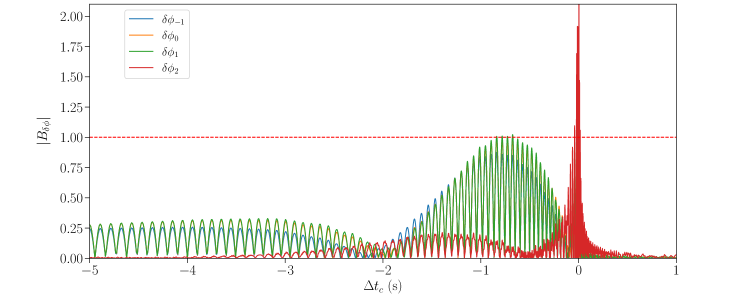
Figure 1: Reduced bias of each PN deviation term as a function of $\Delta t_{c}$, for an OS characterized by parameters in Eq. (15).

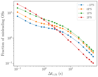
Figure 2: Fraction of misleading OSs for each PN-deviation model against $\Delta t_{c,\rm th}$.

As an illustration, we consider an OS with the following parameters,

$$\mathcal{M}^{(1)} =32\,\mathrm{M}_{\odot}\,,\quad \mathcal{M}^{(2)} =35\,\mathrm{M}_{\odot}\,,$$

$$\eta^{(1)} =0.246\,,\quad \eta^{(2)} =0.248\,,$$

$$d_{L}^{(1)} =10000\,\rm{Mpc}\,,\quad d_{L}^{(2)} =45000\,\rm{Mpc}\,,$$

$$\rm{SNR}^{(1)} =41.74\,,\quad \rm{SNR}^{(2)} =9.96\,.$$ (15)

In Figure 1 we plot the change of the reduced bias with respect to $\Delta t_{c}$ for this OS. It answers our first question in Sec. 1, namely, it is possible that, under the effects of a weaker signal 2, some PN terms of signal 1 possess a reduced bias larger than 1. It is also worth attention that large biases of $-1$PN, 0PN, 1PN coefficients are obtained around $\Delta t_{c}=1\,{\rm s}$, while the bias of $2$PN coefficient has peaked at a much smaller $\Delta t_{c}$ around zero. This can be explained by the fact that the higher order PN terms are mainly prominent in the late inspiral phase of the signal, and we expect the deviation from a higher order PN term to be more significant when $\Delta t_{c}$ between two signals is small.

Simply highlighting a single instance with parameters in Eq. (15) is not sufficient to underscore the risks posed by all OSs, as such instances may be too infrequent to a warrant general concern. To answer the second question in Sec. 1, we generate populations for different $\Delta t_{c,\rm th}$ and calculate the biases for every PN-deviation waveform under consideration. Afterwards, we calculated the fraction of misleading OSs in all OSs in each scenario. The findings are presented in Figure 2. The observation is that the fractions of misleading OSs, defined as $|B_{\delta\phi}|>1$, are around ten percent for populations with small $\Delta t_{c,\rm th}$. Such fractions are not negligible. All fractions then decrease as $\Delta t_{c,\rm th}$ increases, because most signals with strong overlapping features happen at small $\Delta t_{c}$. When $\Delta t_{c,\rm th}$ is large, e.g., larger than 10 s, all fractions are inversely proportional to $\Delta t_{c,\rm th}$. This means that almost all misleading OSs have $\Delta t_{c}\leq 10\,{\rm s}$.

The behaviors of these fractions in Figure 2 at different PN orders are also noteworthy. We note that the fraction of misleading OSs in the 2PN-deviation case is larger than that in the 1PN-deviation case when $\Delta t_{c,\rm th}$ is within $0.5$ s, while for a larger $\Delta t_{c,\rm th}$ it is the opposite. Since the 2PN term is more prominent in the late inspiral phase, it is more likely to generate misleading OSs when $\Delta t_{c}$ is small (as shown in Figure 1), corresponding to a relatively large fraction. As a trade-off, almost all misleading OSs in the 2PN-deviation case have $\Delta t_{c}\lesssim 0.5\,{\rm s}$, corresponding to the quick decrease after $\Delta t_{c,{\rm th}}\simeq 0.5\,$s. In comparison, in the 0PN and 1PN deviation cases, similar behavior of these fractions is observed at $\Delta t_{c,\rm th}$ between 1 s and 10 s. The fraction of misleading OSs in the 1PN-deviation case decreases faster than that at the 0PN order, meaning that the number of misleading OSs in the 0PN deviation case with $1\,{\rm s}<\Delta t_{c}<10\,{\rm s}$ is larger than that in the 1PN-deviation case. However, since $\Delta t_{c}$ is relatively large when the 0PN term dominates the phase evolution, it is difficult to generate large biases, and the total number of misleading OSs in the 1PN-deviation case is still larger than that in the 0PN-deviation case for a large $\Delta t_{c,\rm th}$. In general, for most $\Delta t_{c,\rm th}$, the fraction of large bias in 1PN coefficient stays the highest among the PN-deviation cases we investigate in this work.

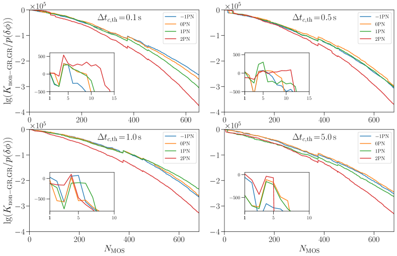
Figure 3: Bayes factor divided by $p(\delta\phi)$ over accumulation of misleading OSs, denoted as $N_{\mathrm{MOS}}$, with different $\Delta t_{c,\rm th}$ for each panel.

From the above findings, we observe a non-negligible proportion of misleading OSs to parameterized PN waveform tests. These OSs, when analyzed individually in tests of GR, tend to favor their respective PN-deviation model more strongly relative to the GR waveform. However, this is not the case when all misleading OSs are considered collectively because of the disagreement on the values of deviation parameters arising from each misleading OS. Figure 3 shows the evolution of Bayes factors of each PN-deviation model against GR with the increase of number of events. For all PN-deviation models, their corresponding Bayes factors exceed 1 only for the first few misleading OSs, and then start drastically decreasing as more misleading OSs enter the test of GR. It is evident that biases in PN deviation terms caused by OSs are not constant as they do not represent a “real” deviation. This is because these biases arise solely from the misclassification of an OS as a single-event signal.

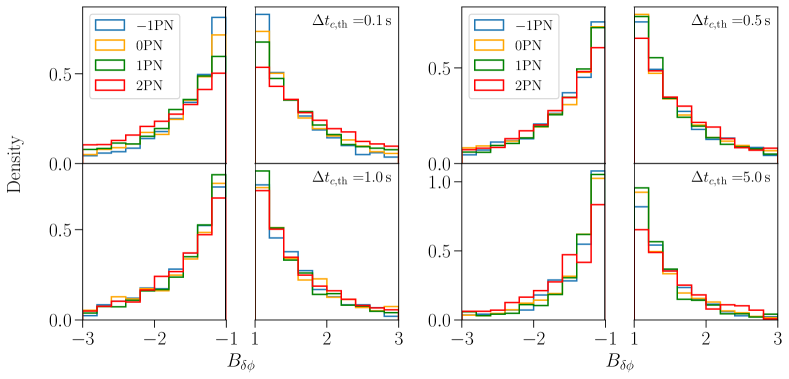
Figure 4: Distribution of large biases of each PN deviation parameter for different $\Delta t_{c,\rm th}$.

However, in our PN-deviation models, the deviation parameters are assumed to be constant. When combining two misleading OSs, where, say, one has the reduced bias $B_{\alpha}>1$ and the other has $B_{\alpha}<-1$, the Bayes factor will rapidly decrease due to the inconsistent biases. To support this, we plot the distribution of reduced biases of the misleading OSs for each PN deviation model in Figure 4, from which we can observe symmetric distributions of reduced biases.

Another interesting aspect noted in Figure 3 is that the Bayes factor for the 2PN deviation model declines more rapidly than those for the $-1$PN, 0PN, and 1PN deviation models, especially at small $\Delta t_{c,\rm th}$. In Figure 4, one can find that the distributions of biases of the $-1$PN, 0PN, and 1PN deviation models cluster more densely near 1, while the distribution for the 2PN deviation model is broader, leading to a greater variance in individual biased values. This is consistent with the argument above that it is more likely to have larger biases in the deviation parameter at the 2PN order. Therefore, the Bayes factor for the 2PN deviation model decreases more rapidly with accumulation of misleading OSs.

5 Conclusions and Discussions

The XG ground-based detectors are anticipated to exhibit a significantly enhanced detection rate of BBHs relative to their forerunners, indicating the unavoidable appearance of OSs in future detection (Regimbau & Hughes, 2009; Meacher et al., 2016; Kalogera et al., 2021). A primary concern regarding such OSs is how they can potentially introduce biases if an OS is mistakenly treated as a single-event signal, thereby misleading parameterized tests of GR. Hu & Veitch (2023) studied the biases in PE when testing GR at the 0PN order with these OSs, and left the comprehensive investigation at different PN orders for future work.

In this work, we extend Hu & Veitch (2023) and investigate how OSs affect $-1$PN to 2PN terms in parameterized tests of GR. We adopt the FM approximation to calculate the biases introduced by OSs. FM is a fast and effective method to study the biases of OSs (Finn, 1992; Antonelli et al., 2021; Hu & Veitch, 2023; Wang et al., 2023). For each PN deviation parameter, we calculate the proportion of signals exhibiting significant bias, and further explore the Bayes factor over accumulation of such misleading OSs. We find that a non-negligible fraction of OSs could produce a significant bias in each PN deviation parameter, especially when the difference in coalescence times, $\Delta t_{c}$, is small. It is worth noting that the fraction of misleading OSs in the 1PN-deviation case is usually the largest, instead of the 0PN-deviation case studied by Hu & Veitch (2023). This underscores the importance of consideration for GR deviations at different PN orders when discussing the impact of OSs on testing gravity.

However, different misleading OSs lead to inconsistent values for deviation parameters, and if analyzed collectively, they do not show a preference for non-GR deviations over GR. This is supported by the decreasing trend of the Bayes factor with an increasing number of misleading OSs, shown in Figure 3.

In real detection, there exist other sources of PE biases when analyzing OSs, such as the waveform modeling (Hu & Veitch, 2023), instrumental calibration (Sun et al., 2020; Hall et al., 2019) and detector glitches (Pankow et al., 2018). We leave a detailed assessment and comparison of all these effects on testing gravity for future work. However, as the misleading OSs discussed, we emphasize the importance of considering the effects at different PN orders to obtain a global understanding.

References

- Abbott et al. (2016) Abbott, B. P., et al. 2016, Phys. Rev. Lett., 116, 061102, doi: 10.1103/PhysRevLett.116.061102
- Abbott et al. (2017a) —. 2017a, Phys. Rev. Lett., 119, 141101, doi: 10.1103/PhysRevLett.119.141101
- Abbott et al. (2017b) —. 2017b, Phys. Rev. Lett., 118, 221101, doi: 10.1103/PhysRevLett.118.221101
- Abbott et al. (2018) —. 2018, Phys. Rev. Lett., 120, 091101, doi: 10.1103/PhysRevLett.120.091101
- Abbott et al. (2019a) —. 2019a, Phys. Rev. X, 9, 031040, doi: 10.1103/PhysRevX.9.031040
- Abbott et al. (2019b) —. 2019b, Phys. Rev. Lett., 123, 011102, doi: 10.1103/PhysRevLett.123.011102
- Abbott et al. (2019c) —. 2019c, Phys. Rev. D, 100, 104036, doi: 10.1103/PhysRevD.100.104036
- Abbott et al. (2019d) —. 2019d, Astrophys. J. Lett., 882, L24, doi: 10.3847/2041-8213/ab3800
- Abbott et al. (2021a) Abbott, R., et al. 2021a. https://arxiv.org/abs/2111.03606
- Abbott et al. (2021b) —. 2021b, Phys. Rev. D, 103, 122002, doi: 10.1103/PhysRevD.103.122002
- Abbott et al. (2021c) —. 2021c. https://arxiv.org/abs/2112.06861
- Abbott et al. (2023) —. 2023, Phys. Rev. X, 13, 011048, doi: 10.1103/PhysRevX.13.011048
- Ando (2004) Ando, S. 2004, JCAP, 06, 007, doi: 10.1088/1475-7516/2004/06/007
- Antonelli et al. (2021) Antonelli, A., Burke, O., & Gair, J. R. 2021, Mon. Not. Roy. Astron. Soc., 507, 5069, doi: 10.1093/mnras/stab2358
- Arun et al. (2006) Arun, K. G., Iyer, B. R., Qusailah, M. S. S., & Sathyaprakash, B. S. 2006, Phys. Rev. D, 74, 024006, doi: 10.1103/PhysRevD.74.024006
- Behroozi & Silk (2015) Behroozi, P. S., & Silk, J. 2015, Astrophys. J., 799, 32, doi: 10.1088/0004-637X/799/1/32
- Belczynski et al. (2006) Belczynski, K., Perna, R., Bulik, T., et al. 2006, Astrophys. J., 648, 1110, doi: 10.1086/505169
- Christensen et al. (2004) Christensen, N., Dupuis, R. J., Woan, G., & Meyer, R. 2004, Phys. Rev. D, 70, 022001, doi: 10.1103/PhysRevD.70.022001
- Christensen & Meyer (1998) Christensen, N., & Meyer, R. 1998, Phys. Rev. D, 58, 082001, doi: 10.1103/PhysRevD.58.082001
- Cornish et al. (2011) Cornish, N., Sampson, L., Yunes, N., & Pretorius, F. 2011, Phys. Rev. D, 84, 062003, doi: 10.1103/PhysRevD.84.062003
- Cutler & Flanagan (1994) Cutler, C., & Flanagan, E. E. 1994, Phys. Rev. D, 49, 2658, doi: 10.1103/PhysRevD.49.2658
- Dominik et al. (2012) Dominik, M., Belczynski, K., Fryer, C., et al. 2012, Astrophys. J., 759, 52, doi: 10.1088/0004-637X/759/1/52
- Dominik et al. (2013) —. 2013, Astrophys. J., 779, 72, doi: 10.1088/0004-637X/779/1/72
- Finn (1992) Finn, L. S. 1992, Phys. Rev. D, 46, 5236, doi: 10.1103/PhysRevD.46.5236
- Ghosh (2022) Ghosh, A. 2022, Summary of Tests of General Relativity with GWTC-3. https://arxiv.org/abs/2204.00662
- Hall et al. (2019) Hall, E. D., Cahillane, C., Izumi, K., Smith, R. J. E., & Adhikari, R. X. 2019, Class. Quant. Grav., 36, 205006, doi: 10.1088/1361-6382/ab368c
- Hild et al. (2011) Hild, S., et al. 2011, Class. Quant. Grav., 28, 094013, doi: 10.1088/0264-9381/28/9/094013
- Himemoto et al. (2021) Himemoto, Y., Nishizawa, A., & Taruya, A. 2021, Phys. Rev. D, 104, 044010, doi: 10.1103/PhysRevD.104.044010
- Hu & Veitch (2023) Hu, Q., & Veitch, J. 2023, Astrophys. J., 945, 103, doi: 10.3847/1538-4357/acbc18
- Janquart et al. (2022) Janquart, J., Baka, T., Samajdar, A., Dietrich, T., & Van Den Broeck, C. 2022. https://arxiv.org/abs/2211.01304
- Kalogera et al. (2021) Kalogera, V., et al. 2021. https://arxiv.org/abs/2111.06990
- Maggiore et al. (2020) Maggiore, M., et al. 2020, JCAP, 03, 050, doi: 10.1088/1475-7516/2020/03/050
- Meacher et al. (2016) Meacher, D., Cannon, K., Hanna, C., Regimbau, T., & Sathyaprakash, B. S. 2016, Phys. Rev. D, 93, 024018, doi: 10.1103/PhysRevD.93.024018
- Meacher et al. (2015) Meacher, D., Coughlin, M., Morris, S., et al. 2015, Phys. Rev. D, 92, 063002, doi: 10.1103/PhysRevD.92.063002
- Mishra et al. (2010) Mishra, C. K., Arun, K. G., Iyer, B. R., & Sathyaprakash, B. S. 2010, Phys. Rev. D, 82, 064010, doi: 10.1103/PhysRevD.82.064010
- Nakar (2007) Nakar, E. 2007, Phys. Rept., 442, 166, doi: 10.1016/j.physrep.2007.02.005
- O’Shaughnessy et al. (2008) O’Shaughnessy, R. W., Kalogera, V., & Belczynski, K. 2008, Astrophys. J., 675, 566, doi: 10.1086/526334
- Pankow et al. (2018) Pankow, C., et al. 2018, Phys. Rev. D, 98, 084016, doi: 10.1103/PhysRevD.98.084016
- Pizzati et al. (2022) Pizzati, E., Sachdev, S., Gupta, A., & Sathyaprakash, B. 2022, Phys. Rev. D, 105, 104016, doi: 10.1103/PhysRevD.105.104016
- Punturo et al. (2010) Punturo, M., et al. 2010, Class. Quant. Grav., 27, 194002, doi: 10.1088/0264-9381/27/19/194002
- Regimbau et al. (2017) Regimbau, T., Evans, M., Christensen, N., et al. 2017, Phys. Rev. Lett., 118, 151105, doi: 10.1103/PhysRevLett.118.151105
- Regimbau & Hughes (2009) Regimbau, T., & Hughes, S. A. 2009, Phys. Rev. D, 79, 062002, doi: 10.1103/PhysRevD.79.062002
- Regimbau et al. (2012) Regimbau, T., et al. 2012, Phys. Rev. D, 86, 122001, doi: 10.1103/PhysRevD.86.122001
- Reitze et al. (2019a) Reitze, D., et al. 2019a, Bull. Am. Astron. Soc., 51, 035. https://arxiv.org/abs/1907.04833
- Reitze et al. (2019b) —. 2019b, Bull. Am. Astron. Soc., 51, 141. https://arxiv.org/abs/1903.04615
- Relton & Raymond (2021) Relton, P., & Raymond, V. 2021, Phys. Rev. D, 104, 084039, doi: 10.1103/PhysRevD.104.084039
- Samajdar et al. (2021) Samajdar, A., Janquart, J., Van Den Broeck, C., & Dietrich, T. 2021, Phys. Rev. D, 104, 044003, doi: 10.1103/PhysRevD.104.044003
- Sathyaprakash et al. (2012) Sathyaprakash, B., et al. 2012, Class. Quant. Grav., 29, 124013, doi: 10.1088/0264-9381/29/12/124013
- Sathyaprakash et al. (2019) Sathyaprakash, B., Buonanno, A., Lehner, L., et al. 2019, Bull. Am. Astron. Soc., 51, 251, doi: 10.48550/arXiv.1903.09221
- Sharma (2017) Sharma, S. 2017, Ann. Rev. Astron. Astrophys., 55, 213, doi: 10.1146/annurev-astro-082214-122339
- Skilling (2004) Skilling, J. 2004, in American Institute of Physics Conference Series, Vol. 735, Bayesian Inference and Maximum Entropy Methods in Science and Engineering, 395, doi: 10.1063/1.1835238
- Skilling (2006) Skilling, J. 2006, Bayesian Analysis, 1, 833, doi: 10.1214/06-BA127
- Sun et al. (2020) Sun, L., et al. 2020, Class. Quant. Grav., 37, 225008, doi: 10.1088/1361-6382/abb14e
- Vallisneri (2008) Vallisneri, M. 2008, Phys. Rev. D, 77, 042001, doi: 10.1103/PhysRevD.77.042001
- Vangioni et al. (2015) Vangioni, E., Olive, K. A., Prestegard, T., et al. 2015, Mon. Not. Roy. Astron. Soc., 447, 2575, doi: 10.1093/mnras/stu2600
- Wang et al. (2023) Wang, Z., Liang, D., Zhao, J., Liu, C., & Shao, L. 2023. https://arxiv.org/abs/2304.06734
- Wang et al. (2022) Wang, Z., Zhao, J., An, Z., Shao, L., & Cao, Z. 2022, Phys. Lett. B, 834, 137416, doi: 10.1016/j.physletb.2022.137416
- Yunes & Pretorius (2009) Yunes, N., & Pretorius, F. 2009, Phys. Rev. D, 80, 122003, doi: 10.1103/PhysRevD.80.122003