Moving Sampling Physics-informed Neural Networks induced by Moving Mesh PDE

Abstract

In this work, we propose an end-to-end adaptive sampling framework based on deep neural networks and the moving mesh method (MMPDE-Net), which can adaptively generate new sampling points by solving the moving mesh PDE. This model focuses on improving the quality of sampling points generation. Moreover, we develop an iterative algorithm based on MMPDE-Net, which makes sampling points distribute more precisely and controllably. Since MMPDE-Net is independent of the deep learning solver, we combine it with physics-informed neural networks (PINN) to propose moving sampling PINN (MS-PINN) and show the error estimate of our method under some assumptions. Finally, we demonstrate the performance improvement of MS-PINN compared to PINN through numerical experiments of four typical examples, which numerically verify the effectiveness of our method.

1 Introduction

In recent years, with the rapid increase in computational resources, solving partial differential equations (PDEs) [19] using deep learning has been an emerging point. Currently, many researchers have proposed widely used deep learning solvers based on deep neural networks, such as the Deep Ritz method [29], which solve the variational problems arising from PDEs; the Deep BSDE model [4], which is developed from stochastic differential equations and performs well at solving high-dimensional problems, and the DeepONet framework [12], which is used to learn operators accurately and efficiently from a relatively small dataset. In this article, we use physics-informed neural networks (PINN) [17]. In PINN, the governing equations of PDEs, boundary conditions, and related physical constraints are incorporated into the design of the loss function, and an optimization algorithm is used to find the network parameters to minimize the loss function, so that the approximated solution output by the neural networks satisfies the governing equations and constraints.

In fact, deep learning solvers need to construct and optimize the loss function. When constructing the loss function, a common choice is the loss function under the $L_{2}$ norm. However, in code-level implementations, it is difficult to compute the loss function directly in integral form, so it is usual to discretize the loss function by sampling uniformly distributed points as empirical loss, commonly known as the mean square error loss function. Ultimately, the optimization algorithm is to minimize the discrete loss function, so the accuracy of the approximation solution is closely related to the accuracy of the discrete loss function. Then, how to choose the sampling points to write the discrete loss function becomes an important problem. There are several uniform sampling methods [27], which include 1) equispaced uniform point sampling, which samples uniformly from the equispaced uniformly distributed points; 2) uniformly random sampling, which randomly samples the points according to a continuous uniform distribution in the computational domain; 3) Latin hypercube sampling [23]; and 4) Sobol sequence ([22],[16]), that is one type of quasi-random low-discrepancy sequence.

There are also many works about non-uniform adaptive sampling methods. Lu et al. in [13] proposed a new residual-based adaptive refinement (RAR) method to improve the training efficiency of PINNs. That is, training points are adaptively added where the residual loss is large. In [3], a selection network is introduced to serve as a weight function to assign higher weights for samples with large point-wise residuals, which yields a more accurate approximate solution if the selection network is properly chosen. In [27], the residual-based adaptive distribution (RAD) method is proposed, and its main idea is to construct a probability density function based on residual information and to adopt adaptive sampling based on this density function. In [15], collocation points are sampled according to a distribution proportional to the loss function in each training iteration. In [24], Tang et al. proposed a deep adaptive sampling method for solving partial differential equations from the perspective of the variance of the residual loss term. All of these adaptive sampling methods above are from the perspective of the loss function, and we would like to focus more on the performance of the solution function. This reminds us of the mesh movement method in traditional numerical methods.

One obvious characteristic of the moving mesh method is that only the mesh nodes are relocated without changing the mesh topology [9], i.e., the number of points of the mesh is fixed before and after the mesh is redistributed. In this paper, we focus on the moving mesh PDE (MMPDE) method [8]. The purpose of the MMPDE method is to provide a system of partial differential equations to control the movement of the mesh nodes. By adjusting the monitor function in MMPDE, the mesh can be made centralized or dispersed which depending on the performance of the solution. Compared with the uniform mesh, the number of nodes in the moved mesh is greatly reduced with the same numerical solution accuracy, thus the efficiency is improved greatly ([5]). In this work, based on the MMPDE method, we propose the adaptive sampling neural network, MMPDE-Net, which is independent of the deep learning solver. It is essentially a coordinate transformation mapping, which enables the coordinates of the output points to be concentrated in the region where the function has large variations. In [18], Ren and Wang proposed an iterative method to generate the mesh. Inspired by this approach, we also develop an iterative algorithm on MMPDE-Net to make the distribution of the sampling points more precise and controllable.

Since MMPDE-Net is essentially a coordinate transformer independent of solving the physical problem, it can be combined with many deep learning solvers. In this work, we choose the most widely used Physically Informed Neural Networks (PINN). We propose a deep learning framework: Moving Sampling PINN (MS-PINN), whose main idea is to use the preliminary solution provided by PINN to help MMDPE-Net develop the monitor function, and then accelerate the convergence of the loss function of PINN through the adaptive sampling points obtained by MMPDE-Net. Meanwhile, with some reasonable assumptions we prove that the error bounds of the approximation solution and the true solution are lower than that of the traditional PINN under a certain probability. Finally, we verify the effectiveness of MS-PINN using the numerical experiments.

In summary, our main contributions in this article are:

• A deep adaptive sampling framework (MMPDE-Net) that adaptively generates new sample points by solving the Moving Mesh PDE is proposed.

• A deep learning framework (MS-PINN) is presented. The core idea is to improve the approximate solution of PINN by adaptive sampling through MMPDE-Net.

• An error estimate of the proposed MS-PINN is given. The effectiveness is demonstrated by reducing the error bounds between the approximate solution and true solution.

The rest of the paper is organized as follows. In Section 2, the main idea of PINN is briefly introduced and a typical example is used to underline the importance of adaptive sampling. In Section 3, MMPDE-Net and the iterative algorithm based on MMPDE-Net are illustrated. The MS-PINN framework is presented and the error estimates are given in Section 4. Numerical experiments are shown in Section 5 to verify the effectiveness of our method. Finally, conclusions are given in Section 6.

2 Preliminary Work

2.1 A brief introduction to PINN

We consider a general form of partial differential equations

$$\left\{\begin{aligned} \mathcal{A}[\bm{u}(\bm{x})]&=f(\bm{x}),\quad\bm{x}\in\Omega,\\ \mathcal{B}[\bm{u}(\bm{x})]&=g(\bm{x}),\quad\bm{x}\in\partial\Omega,\end{aligned}\right.$$ (1)

where $\Omega\subset\mathbb{R}^{d}$ is a bounded, open and connected domain which has a polygonal boundary $\partial\Omega$, $\mathcal{A}$ is a partial differential operator, $f(\bm{x})$ is the source function, $\mathcal{B}$ and $g(\bm{x})$ are the boundary operator and the boundary condition.

As stated above, the core idea of PINN is to incorporate the equation itself and its constraints into the design of the loss function. Suppose the approximate solution output by PINN is $\bm{u}(\bm{x};\theta)$, $\mathcal{A}[\bm{u}(\bm{x};\theta)]-f(\bm{x})\in L^{2}(\Omega)$ and $\mathcal{B}[\bm{u}(\bm{x};\theta)]-g(\bm{x})\in L^{2}(\partial\Omega)$, the loss function can be written as

$$\mathcal{L}(\bm{x};\theta) =\alpha_{1}\|\mathcal{A}[\bm{u}(\bm{x};\theta)]-f(\bm{x})\|_{2,\Omega}^{2}+\alpha_{2}\|\mathcal{B}[\bm{u}(\bm{x};\theta)]-g(\bm{x})\|_{2,\partial\Omega}^{2}$$ (2)

$$=\alpha_{1}\int_{\Omega}|\mathcal{A}[\bm{u}(\bm{x};\theta)]-f(\bm{x})|^{2}d\bm{x}+\alpha_{2}\int_{\partial\Omega}|\mathcal{B}[\bm{u}(\bm{x};\theta)]-g(\bm{x})|^{2}d\bm{x}$$

$$\triangleq\alpha_{1}\int_{\Omega}|r(\bm{x};\theta)|^{2}d\bm{x}+\alpha_{2}\int_{\partial\Omega}|b(\bm{x};\theta)|^{2}d\bm{x},$$

where $\theta\in\mathbb{R}^{NN}$ represents the parameters of the neural networks, usually consisting of weights and biases, and $\mathbb{R}^{NN}$ is the space determined by the structure of the neural network, $\alpha_{1}$ is the weight of the residual loss term and $\alpha_{2}$ is the weight of the boundary loss term. Typically, when discretizing the loss function Eq (2), we sample uniformly distributed residual training points $\left\{\bm{x}_{i}\right\}_{i=1}^{M_{r}}\subset\Omega$ and boundary training points $\left\{\bm{x}_{i}\right\}_{i=1}^{M_{b}}\subset\partial\Omega$, and the empirical loss is written as

$$\mathcal{L}_{M}(\bm{x};\theta)=\frac{\alpha_{1}}{M_{r}}\sum_{i=1}^{M_{r}}|r(\bm{x}_{i};\theta)|^{2}+\frac{\alpha_{2}}{M_{b}}\sum_{i=1}^{M_{b}}|b(\bm{x}_{i};\theta)|^{2}.$$ (3)

After that, optimization algorithms such as Adam [10] and LBFGS [11] are used to make the value of $\mathcal{L}_{M}(\bm{x};\theta)$ in Eq (3) decrease gradually during the training process. When the value of $\mathcal{L}_{M}(\bm{x};\theta)$ is small enough, the solution $\bm{u}(\bm{x};\theta)$ output by the neural networks can be regarded as the approximate solution with a sufficiently small error ([20],[21]).

2.2 A discussion of a certain solution

Consider the following one-dimensional example

$$\begin{array}[]{r@{}l}\left\{\begin{aligned} &-u_{xx}(\bm{x})=f(\bm{x}),\quad\bm{x}\in\Omega,\\ &u(\bm{x})=g(\bm{x}),\quad\bm{x}\in\partial\Omega,\\ \end{aligned}\right.\end{array}$$ (4)

where the computational domain $\Omega=(0,3\pi)$. For a given $f(x)$, the analytical solution of Eq (4) is

$$u(\bm{x})=e^{-2(x-4)(x-5)}\sin(kx),$$ (5)

where $k\in\mathbb{N}$ is a parameter. It is well known that the analytical solution $u(\bm{x})$ vibrates up and down more and more frequently on $[\pi,2\pi]$ as the frequency $k$ becomes larger.

Now, we use PINN to solve this problem and uniformly sample $M_{r}=300$ points in the computational region $\Omega$ as the residual training set. For the boundary training points, there are only left and right endpoints $M_{b}=2$. We take 4 hidden layers with 60 neurons per layer and use tanh as the activation function. The Adam optimization method is used and the initial learning rate is 0.0001. The loss function is defined as follows

$$\mathcal{L}oss(\bm{x};\theta)=\frac{1}{M_{r}}\sum_{i=1}^{M_{r}}|-\Delta u(\bm{x};\theta)-f(\bm{x})|^{2}+\frac{1}{M_{b}}\sum_{i=1}^{M_{b}}|u(\bm{x};\theta)-g(\bm{x})|^{2},$$ (6)

where the weights $\alpha_{1}=1$ and $\alpha_{2}=1$. The minimum value of the loss function and the error $e_{2}(u)$ are given in Table 1, where $e_{2}(u)$ is defined in Section 5.1. It is clear that the values of the loss function and the error become larger as $k$ increases.

Table 1: Variation of the minimum of the loss function and the relative error between the approximate solution and analytical solution for different frequency $k$ with $20000$ training epochs.

k	2	4	6	8
Loss	$1.033\times 10^{-5}$	$8.530\times 10^{-5}$	$1.215\times 10^{-4}$	1.244
$e_{2}(u)$	$3.301\times 10^{-4}$	$2.843\times 10^{-3}$	$2.284\times 10^{-3}$	$1.201\times 10^{-1}$

Since the behavior of the solution varies in different regions, now we let the numbers of sampling points on $(0,\pi]$ and $[2\pi,3\pi)$ are fixed, i.e., $M_{r1}$ and $M_{r3}$ are fixed, and only the number of sampling points on $[\pi,2\pi]$ is increased, i.e., $M_{r2}$ changes. For frequency $k=16$, the number of sampling points ($M_{r}=M_{r1}+M_{r2}+M_{r3}$, $M_{r1}=M_{r3}=100$, $M_{r2}=100,150,250,300$) is varied with 10000 epochs and 20000 epochs. It is easy to observe from Fig 1 that in the region with large vibrations, more sampling points in $[\pi,2\pi]$ tend to make the loss function decrease fast and help the neural networks to learn the solution.

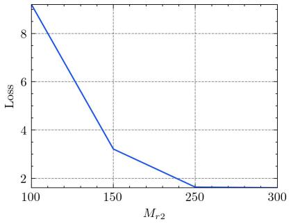
(a) epochs N=10000

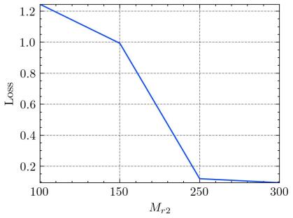
(b) epochs N=20000

Figure 1: Variation of the minimum of the loss function with different number of sampling points ($M_{r2}$ =100,150,250,300) for $k=16$.

In fact, there are similar results in [2], where 1D sine function of frequency $k$ is learned in time $O\left(\frac{k^{2}}{\rho}\right)$, and $\rho$ denotes the minimum sampling density in the input space. If we regard the parameter $\theta$ of the neural networks as a random variable, for the empirical loss Eq (3) we define the loss function expectation $\mathbb{E}_{\theta}\left[\mathcal{L}_{M}(\bm{x};\theta)\right]$. From the results shown in Fig 1, we consider the loss function expectation $\mathbb{E}_{\theta}\left[\mathcal{L}_{M}(\bm{x};\theta)\right]$ positively related to the function frequency $k$ and negatively related to the number of sampling points. That is, when the frequency of the learning function is fixed, the more sampling points, the smaller $\mathbb{E}_{\theta}\left[\mathcal{L}_{M}(\bm{x};\theta)\right]$ is, regardless of the location of the sampling points.

In the following, we use $k$ to denote the complexity (e.g. frequency) of the solution. In order to further study the effect of the complexity of the solution and the number of sampling points on the loss function, we rewrite the residual loss expectation in Definition 1.

Definition 1.

For $\forall M_{r},M\in\mathbb{N^{+}},M\leq M_{r}$ and $\forall k>0$, the residual loss expectation in a certain subregion(region) is defined as

$$\mathcal{F}(k,M,M_{r})=\mathbb{E}_{\theta}\left[\frac{1}{M_{r}}\sum_{i=1}^{M}|r(x_{i};\theta|^{2}\right],$$ (7)

where $\mathbb{N^{+}}$ denotes the set of positive integers.

Remark 1.

In different subrange $\Omega_{i}$, where $\Omega=\{\Omega_{i}\}_{i=1}^{N_{k}}$, the complexity $k_{i}$ of the solution is different and $\bm{k}=\{{k_{i}}\}_{i=1}^{N_{k}}$, therefore the number of sampling points ${M_{i}}$ in different subregion is different. We have

$$\mathcal{F}(k,M_{r},M_{r})=\sum_{i=1}^{N_{k}}\mathcal{F}(k_{i},M_{i},M_{r}),\quad\mbox{where}\quad\sum_{i=1}^{N_{k}}M_{i}=M_{r}.$$ (8)

In order to establish the error estimate, we give Assumption 1 following the reference [2].

Assumption 1.

$\forall k,\alpha,\beta>0,\forall M\leq M_{r}\in\mathbb{N^{+}}$, $\exists$ $p,q>0$, s.t.,

$$\mathcal{F}(\alpha k,M,M_{r})=\alpha^{p}\mathcal{F}(k,M,M_{r}),\quad\mathcal{F}(k,\beta M,M_{r})=\frac{1}{\beta^{q}}\mathcal{F}(k,M,M_{r}),$$

which is due to the positively relation of the function complexity $k$ and the negatively relation of the number of sampling points $M$.

3 Implement of MMPDE-Net

3.1 MMPDE-Net

In this section, our goal is to develop the neural networks that are independent of the problem and used only for adaptive sampling. We would like to concentrate the sampling points as much as possible on the regions where the behaviors of the solution are intricate. This is similar to the idea of the moving mesh PDE (MMPDE) in the traditional numerical methods. Firstly, we briefly introduce the MMPDE derivation in two-dimensional case. Let’s define a one-to-one coordinate transformation on $\Omega\subset\mathbb{R}^{2}$

$$\bm{x}=\bm{x}(\bm{\xi}),\quad\forall\bm{\xi}=(\xi,\eta)\in\Omega,$$ (9)

where $\bm{\xi}=(\xi,\eta)$ represents the coordinates before transformation and $\bm{x}=(x,y)$ represents the coordinates after transformation.

The mesh functional in variational approach can usually be expressed in the form

$$E(\bm{\xi})=\int_{\Omega}\sum_{i,j,\alpha,\beta}w^{i,j}\frac{\partial\bm{\xi}^{\alpha}}{\partial\bm{x}^{i}}\frac{\partial\bm{\xi}^{\beta}}{\partial\bm{x}^{j}}d\bm{x},$$ (10)

where $W=(w_{i,j}),W^{-1}=(w^{i,j})$ are symmetric positive definite matrices that are monitor functions in a matrix form. According to Winslow’s variable diffusion method [26], a special case of Eq (10) is defined as follows

$$E(\xi,\eta)=\int_{\Omega}\ \frac{1}{w}\left(|\nabla\xi|^{2}+|\nabla\eta|^{2}\right)dxdy,$$ (11)

where $\nabla=\left(\frac{\partial}{\partial x},\frac{\partial}{\partial y}\right)^{T}$, $w$ is a monitor function that depends on the solution. The Euler–Lagrange equation whose solution minimizes Eq (11) is as follows

$$\left\{\begin{aligned} \nabla\left(\frac{1}{w}\nabla\xi\right)=0,\\ \nabla\left(\frac{1}{w}\nabla\eta\right)=0,\end{aligned}\right.$$ (12)

which can be regarded as a steady state of the heat flow equation Eq (13)

$$\left\{\begin{aligned} \frac{\partial\xi}{\partial t}-\nabla\left(\frac{1}{w}\nabla\xi\right)=0,\\ \frac{\partial\eta}{\partial t}-\nabla\left(\frac{1}{w}\nabla\eta\right)=0.\end{aligned}\right.$$ (13)

Interchanging the dependent and independent variables in Eq (13), we have

$$\begin{split}(x_{t},y_{t})^{T}=-\frac{(x_{\xi},y_{\xi})^{T}}{J}\left\{\frac{\partial}{\partial\xi}\left((x_{\eta},y_{\eta})\frac{1}{Jw}(x_{\eta},y_{\eta})^{T}\right)-\frac{\partial}{\partial\eta}\left((x_{\xi},y_{\xi})\frac{1}{Jw}(x_{\eta},y_{\eta})^{T}\right)\right\}\\ -\frac{(x_{\eta},y_{\eta})^{T}}{J}\left\{-\frac{\partial}{\partial\xi}\left((x_{\eta},y_{\eta})\frac{1}{Jw}(x_{\xi},y_{\xi})^{T}\right)+\frac{\partial}{\partial\eta}\left((x_{\xi},y_{\xi})\frac{1}{Jw}(x_{\xi},y_{\xi})^{T}\right)\right\}.\end{split}$$ (14)

where $J=x_{\xi}y_{\eta}-x_{\eta}y_{\xi}$.

The neural networks can be treated as a coordinate transformation, as in Eq (9). An intuitive idea is to solve Eq (14) with input $(\xi,\eta)$ and output $(x,y)$. We denote that

$$\left\{\begin{aligned} \mathcal{S}_{1}(x,y,\xi,\eta,J,w)=&\frac{\partial}{\partial\xi}\left((x_{\eta},y_{\eta})\frac{1}{Jw}(x_{\eta},y_{\eta})^{T}\right)-\frac{\partial}{\partial\eta}\left((x_{\xi},y_{\xi})\frac{1}{Jw}(x_{\eta},y_{\eta})^{T}\right),\\ \mathcal{S}_{2}(x,y,\xi,\eta,J,w)=&-\frac{\partial}{\partial\xi}\left((x_{\eta},y_{\eta})\frac{1}{Jw}(x_{\xi},y_{\xi})^{T}\right)+\frac{\partial}{\partial\eta}\left((x_{\xi},y_{\xi})\frac{1}{Jw}(x_{\xi},y_{\xi})^{T}\right).\end{aligned}\right.$$ (15)

Using Eq (15), Eq (14) is rewritten as

$$\left\{\begin{aligned} x_{t}&+\frac{x_{\xi}}{J}\mathcal{S}_{1}(x,y,\xi,\eta,J,w)+\frac{x_{\eta}}{J}\mathcal{S}_{2}(x,y,\xi,\eta,J,w)=0,\quad(\xi,\eta)\in\Omega,\\ y_{t}&+\frac{y_{\xi}}{J}\mathcal{S}_{1}(x,y,\xi,\eta,J,w)+\frac{y_{\eta}}{J}\mathcal{S}_{2}(x,y,\xi,\eta,J,w)=0,\quad(\xi,\eta)\in\Omega,\\ x&=\xi,y=\eta,\quad(\xi,\eta)\in\partial\Omega.\\ \end{aligned}\right.$$ (16)

Now we establish the neural networks to solve Eq (16). When dealing with time discretization, we use the forward Euler formula. There are still two issues to be addressed. One is to define the monitor function $w(\xi,\eta)$, the other is to enforce the boundary conditions.

In traditional numerical methods, the role of the monitor function is to guide the movement of the mesh points so that they are concentrated in the region where the monitor function is large. Since MMPDE-Net is independent of solving equations, we need to know some prior knowledge about the solution. When dealing with boundary conditions, instead of adding loss terms of the boundary conditions as in PINN, we utilize the enforcement approach([28],[14]). The fully connected neural networks is employed as our network architecture. We assume that the sampled training points are $\left\{(\xi_{i},\eta_{i})\right\}_{i=1}^{M}$, then the loss function of the MMPDE is given by

$$\mathcal{L}oss_{MMPDE}\left((\xi,\eta);\theta\right)$$ (17)

$$=\frac{1}{M}\sum_{i=1}^{M}\left|\frac{x_{i}-\xi_{i}}{\tau}+\frac{x_{\xi}(\xi_{i},\eta_{i})}{J}\mathcal{S}_{1}(x,y,\xi_{i},\eta_{i},J,w)+\frac{x_{\eta}(\xi_{i},\eta_{i})}{J}\mathcal{S}_{2}(x,y,\xi_{i},\eta_{i},J,w)\right|^{2}$$

$$+\frac{1}{M}\sum_{i=1}^{M}\left|\frac{y_{i}-\eta_{i}}{\tau}+\frac{y_{\xi}(\xi_{i},\eta_{i})}{J}\mathcal{S}_{1}(x,y,\xi_{i},\eta_{i},J,w)+\frac{y_{\eta}(\xi_{i},\eta_{i})}{J}\mathcal{S}_{2}(x,y,\xi_{i},\eta_{i},J,w)\right|^{2}.$$

MMPDE-Net is described in Algorithm 1 for the two-dimensional problem, and a flowchart of the computational process is given in Fig 2.

Symbols: Maximum epoch number of MMPDE-Net $N_{1}$; the number of total points $M_{r}$; initial training points $\mathcal{X}:=\left\{(\xi_{k},\eta_{k})\right\}_{k=1}^{M_{r}}\subset\Omega$; parameter $\tau$ in Eq (17).

Constructing the monitor function:

Given the sampling points $\mathcal{X}$.

Utilizing prior knowledge to obtain $[u(\mathcal{X}),\nabla u(\mathcal{X}),...]$.

Construct the monitor function $w[u(\mathcal{X}),\nabla u(\mathcal{X}),...]$, abbreviated as $w(u(\mathcal{X}))$.

Adaptive Sampling:

Input $\mathcal{X}$ into neural networks.

Initialize the output $\tilde{\mathcal{X}}:=\tilde{\mathcal{X}}(\mathcal{X};\theta^{0})$.

for $i=0:N_{1}-1$ do

      

      $\mathcal{L}oss[\tilde{\mathcal{X}}(\mathcal{X};\theta^{i});w(u(\mathcal{X}))]=\mathcal{L}oss_{MMPDE}(\mathcal{X};\theta^{i})$ (Eq (17));

      Update $\theta^{i+1}$ by descending the gradient of $\mathcal{L}oss[\tilde{\mathcal{X}}(\mathcal{X};\theta^{i});w(u(\mathcal{X}))]$.

end for

Output the new training points $\tilde{\mathcal{X}}=\tilde{\mathcal{X}}(\mathcal{X};\theta^{N_{1}})=\left\{(x_{k},y_{k})\right\}_{k=1}^{M_{r}}$.

Algorithm 1 Algorithm of MMPDE-Net in the 2D case

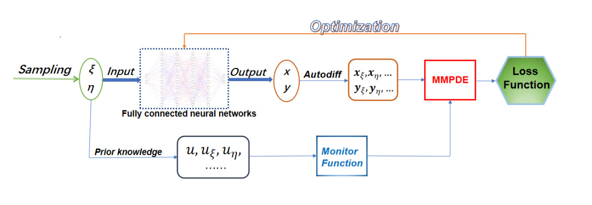
Figure 2: Flow chart of MMPDE-Net.

Now we consider solution function $u=ce^{-c^{2}{(x^{2}+y^{2})}}$ and the monitor function $w=(1+u^{2})^{\frac{1}{2}}$. The uniform sampling points are input into MMPDE-Net. The output of MMPDE-Net for $c=5,10,50,100$ are shown in Fig 3. It can be seen the distribution of sampling points is clearly more concentrated on the place where the function value is large, which is due to the effect of the monitor function. In Fig 4, we consider function $u=e^{-(4x^{2}+9y^{2}-1)^{2}}$. It is obvious to see that the gradient of solution is important and the monitor function is taken as $w=(1+(\lvert\nabla u\rvert)^{2})^{\frac{1}{2}}$. The gradient of $u$ and the distribution of sampling points are shown in Fig 4.

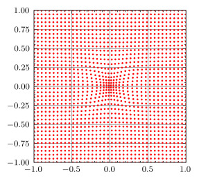
(a) c =5

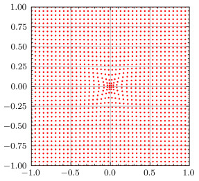
(b) c =10

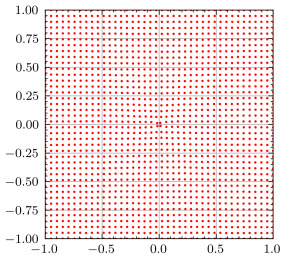
(c) c =50

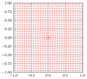
(d) c =100

Figure 3: Points distribution for $u=ce^{-c^{2}{(x^{2}+y^{2})}}$ and $w=(1+u^{2})^{\frac{1}{2}}$ in 2D case when $c$ is increased. (a) $c=5$; (b) $c=10$; (c) $c=50$; (d) $c=100$.

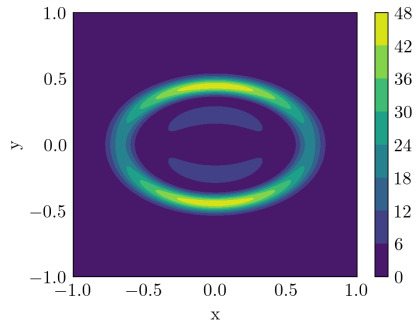
(a) $\nabla u$

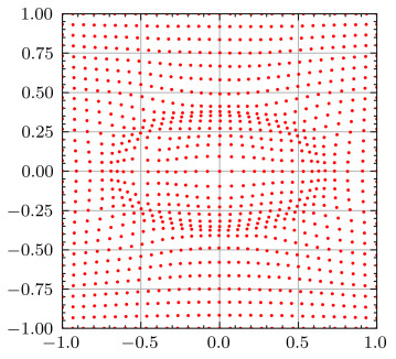
(b) new distribution of sampling points

Figure 4: (a) the gradient of $u=e^{-(4x^{2}+9y^{2}-1)^{2}}$; (b) points distribution with $w=(1+(\lvert\nabla u\rvert)^{2})^{\frac{1}{2}}$.

As in Section 2.2, the $\bm{k}$ is denoted as the complexity of the solution $u$. After using MMPDE-Net, the sampling points obey the distribution $\bm{x}\sim\rho(\bm{k};\bm{x})$ induced by the monitor function $w(\bm{k};\bm{x})$ and MMPDE Eq (14), where $\rho(\bm{k};\bm{x})$ is a probability density function (PDF), i.e., $\int_{\Omega}\rho(\bm{k};\bm{x})d\bm{x}=1$ and $\rho(\bm{k};\bm{x})\geq 0$. As a result, the sampling points are distributed in the region where the monitor function $w(\bm{k};\bm{x})$ is large, i.e., enough points are sampled from the PDF $\rho(\bm{k};\bm{x})$.

3.2 MMPDE-Net with iterations

An iterative method for moving mesh is proposed in [18]. The iteration of the grid generation allows us to more precisely control the grid distribution in the regions where the solution has large variations. In this section, we introduce the iterative algorithm for MMPDE-Net.

Since new sampling points are generated in each iteration based on the old ones, i.e., a one-to-one coordinate transformation is implemented in each iteration, which corresponds to performing the training of MMPDE-Net. It is worth noting that at each training of MMPDE-Net, we need to formulate the monitor function based on the most recent input training points and reinitialize the parameters of the neural networks. MMPDE-Net with iterations is described in Algorithm 2 for the 2D case.

Symbols: Maximum epoch number of MMPDE-Net $N_{1}$; the number of total points $M_{r}$; initial training points $\mathcal{X}_{0}:=\left\{(\xi_{k},\eta_{k})\right\}_{k=1}^{M_{r}}\subset\Omega$; maximum number of iterations $N_{it}$; parameter $\tau$ in Eq (17).

for $j=0:N_{it}-1$ do

       Constructing the monitor function:

       Given the sampling points $\mathcal{X}_{j}$.

      Utilizing prior knowledge to obtain $[u(\mathcal{X}_{j}),\nabla u(\mathcal{X}_{j}),...]$.

      Construct the monitor function $w[u(\mathcal{X}_{j}),\nabla u(\mathcal{X}_{j}),...]$, abbreviated as $w(u(\mathcal{X}_{j}))$.

      Adaptive Sampling:

       Input $\mathcal{X}_{j}$ into neural networks.

      Initialize the output $\tilde{\mathcal{X}}:=\tilde{\mathcal{X}}(\mathcal{X}_{j};\theta^{0}_{j})$.

      for $i=0:N_{1}-1$ do

            

            $\mathcal{L}oss[\tilde{\mathcal{X}}(\mathcal{X}_{j};\theta^{i}_{j});w(u(\mathcal{X}_{j}))]=\mathcal{L}oss_{MMPDE}(\mathcal{X}_{j};\theta^{i}_{j})$ (Eq (17));

            Update $\theta^{i+1}_{j}$ by descending the gradient of $\mathcal{L}oss[\tilde{\mathcal{X}}(\mathcal{X}_{j};\theta^{i}_{j});w(u(\mathcal{X}_{j}))]$.

       end for

      

      Output the new training points $\tilde{\mathcal{X}}=\tilde{\mathcal{X}}(\mathcal{X}_{j};\theta^{N_{1}}_{j})$.

      Update $\mathcal{X}_{j+1}=\tilde{\mathcal{X}}$.

end for

Output the final training points $\mathcal{X}_{N_{it}}:=\tilde{\mathcal{X}}(\mathcal{X}_{0};\theta^{N_{1}}_{0},\theta^{N_{1}}_{1},...,\theta^{N_{1}}_{N_{it}-1})=\left\{(x_{k},y_{k})\right\}_{k=1}^{M_{r}}$.

Algorithm 2 Algorithm of MMPDE-Net with iterations in the 2D case

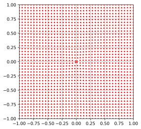
(a) 1 iteration

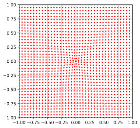
(b) 2 iterations

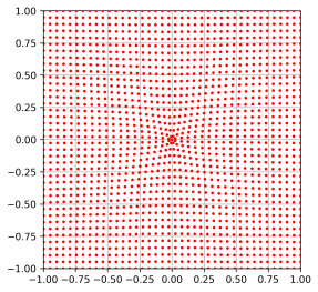
(c) 3 iterations

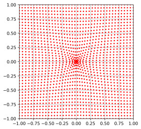
(d) 5 iterations

Figure 5: Points distribution for $u=50e^{-c^{2}{(x^{2}+y^{2})}}$ and $w=(1+u^{2})^{\frac{1}{2}}$ after iterations. (a) after 1 iteration; (b) after 2 iterations; (c) after 3 iterations; (d) after 5 iterations.

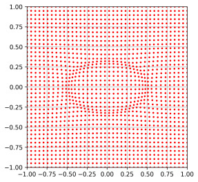
(a) 1 iteration

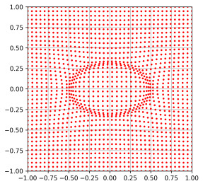
(b) 2 iterations

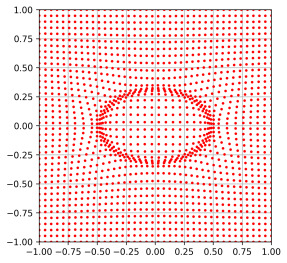
(c) 3 iterations

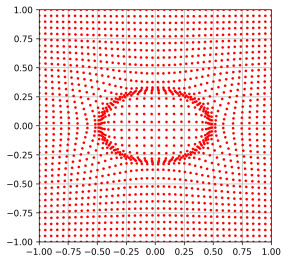
(d) 4 iterations

Figure 6: Points distribution for $u=e^{-8{(4x^{2}+9y^{2}-1)^{2}}}$ and $w=1+u$ after several iterations. (a) after 1 iteration; (b) after 2 iterations; (c) after 3 iterations; (d) after 4 iterations.

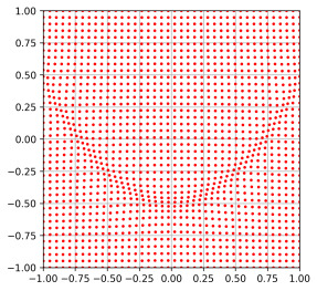
(a) 1 iteration

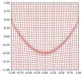
(b) 2 iterations

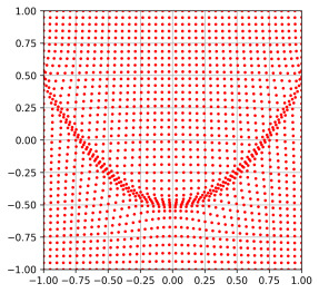
(c) 3 iterations

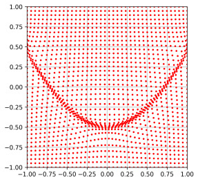
(d) 4 iterations

Figure 7: Points distribution for $u=e^{-100{(-x^{2}+y+0.5)^{2}}}$ and $w=1+u$ after several iterations. (a) after 1 iteration; (b) after 2 iterations; (c) after 3 iterations; (d) after 4 iterations.

In Fig 5, 6 and 7, we reproduce the numerical results in [18] about mesh iterations. In these figures, the monitor function is given and only iteration number varies. It can be seen that as the iterations increase, the distribution of points behaves more and more concentrated which is due to the monitor function. In fact, this iterative process with a well-chosen monitor function can be repeated until the concentration at the sampling point is satisfactory [18], as long as the loss function Eq (17) can be optimized.

4 Implement of MS-PINN

4.1 MS-PINN

Since MMPDE-Net is essentially a coordinate transformation mapping, it can be combined with many deep learning solvers, in this work we choose PINN, which is one of the most widely used neural networks.

It is not straightforward to embed MMPDE-Net into PINN, for example, by adding loss Eq (17) to the loss of PINN, which would not only make the loss function more difficult to optimize, but also reduce the efficiency of training. The combination should be a mutually beneficial relationship: PINN will feed MMPDE-Net the prior information about the solution to help to define the monitor function; MMPDE-Net will feed new sampling points back to PINN to output better approximate solutions.

Denote $\theta_{P}$ and $\theta_{MM}$ as the parameters of PINN and MMPDE-Net respectively, the training of MS-PINN is divided into three stages:

• The pre-training with PINN. The input is the initial sampling points $\mathcal{X}$, and after a small number $N_{1}$ epochs of training, the output is the information of the solution on the initial training points $u(\mathcal{X};\theta_{P}^{N_{1}}),\nabla u(\mathcal{X};\theta_{P}^{N_{1}}),...$.

• The adaptive sampling with MMPDE-Net. The input is the initial sampling points $\mathcal{X}$, at the same time, we use the outputs of PINN from the pre-training stage to define the monitor function $w[u(\mathcal{X};\theta_{P}^{N_{1}}),\nabla u(\mathcal{X};\theta_{P}^{N_{1}}),...)]$, abbreviated by $w(u(\mathcal{X};\theta_{P}^{N_{1}}))$, and the output is the new sampling points after the coordinate transformation $\tilde{\mathcal{X}}=\tilde{\mathcal{X}}(\mathcal{X};\theta_{P}^{N_{1}},\theta_{MM}^{N_{2}})$.

• The formal training with PINN. The input is the new sampling points $\tilde{\mathcal{X}}$ and after $N_{3}$ epochs of training, the output is the solution at the new sampling points $u(\tilde{\mathcal{X}};\theta_{P}^{N_{3}})$.

It is worth noting that in the formal training stage, we do not reinitialize the parameters of PINN, but inherit the parameters obtained from the pre-training, which does help the convergence of the loss function. Moreover, the loss functions of MMPDE-Net and PINN are independent; the loss function of MMPDE-Net is in the form of Eq (17) which consists of only one loss term based on MMPDE; the loss function of PINN is in the form of Eq (3), which generally consists of a residual loss term and a boundary loss term.

Symbols: Maximum epoch number of pre-training, MMPDE-Net and formal training: $N_{1}$, $N_{2}$ and $N_{3}$; the numbers of total points in $\Omega$ and $\partial\Omega$: $M_{r}$, and $M_{b}$; initial training points $\mathcal{X}:=\left\{(\xi_{k},\eta_{k})\right\}_{k=1}^{M_{r}}\subset\Omega$ and $\mathcal{X}_{b}:=\left\{(\xi_{k},\eta_{k})\right\}_{k=1}^{M_{b}}\subset\partial\Omega$; points in the test set $\mathcal{X}_{T}:=\left\{(\xi_{k}^{T},\eta_{k}^{T})\right\}_{k=1}^{M_{T}}\subset\Omega\cup\partial\Omega$; the number of test set points $M_{T}$; $\theta_{P}$ and $\theta_{MM}$ are the parameters of PINN and MMPDE-Net respectively; parameter $\tau$ in Eq (17).

Pre-training:

Input $\mathcal{X}$ and $\mathcal{X}_{b}$ into PINN.

Initialize the output $u(\mathcal{X},\mathcal{X}_{b};\theta_{P}^{0})$.

for $i=0:N_{1}-1$ do

      

      $\mathcal{L}oss[u(\mathcal{X},\mathcal{X}_{b};\theta_{P}^{i})]:=\mathcal{L}oss_{res}(\mathcal{X};\theta_{P}^{i})+\mathcal{L}oss_{bou}(\mathcal{X}_{b};\theta_{P}^{i})$;

      Update $\theta_{P}^{i+1}$ by descending the gradient of $\mathcal{L}oss[u(\mathcal{X},\mathcal{X}_{b};\theta_{P}^{i})]$.

end for

Output $u(\mathcal{X};\theta_{P}^{N_{1}}),\nabla u(\mathcal{X};\theta_{P}^{N_{1}}),...$.

Construct the monitor function $w[u(\mathcal{X};\theta_{P}^{N_{1}}),\nabla u(\mathcal{X};\theta_{P}^{N_{1}}),...)]$, abbreviated as $w(u(\mathcal{X};\theta_{P}^{N_{1}}))$.

Adaptive Sampling:

Input $\mathcal{X}$ into MMPDE-Net.

Initialize the output $\tilde{\mathcal{X}}:=\tilde{\mathcal{X}}(\mathcal{X};\theta_{MM}^{0})$.

for $i=0:N_{2}-1$ do

      

      $\mathcal{L}oss[\tilde{\mathcal{X}}(\mathcal{X};\theta_{MM}^{i});w(u(\mathcal{X};\theta_{P}^{N_{1}}))]=\mathcal{L}oss_{MMPDE}(\mathcal{X};\theta_{MM}^{i})$ (Eq (17));

      Update $\theta_{MM}^{i+1}$ by descending the gradient of $\mathcal{L}oss[\tilde{\mathcal{X}}(\mathcal{X};\theta_{MM}^{i});w(u(\mathcal{X};\theta_{P}^{N_{1}}))]$.

end for

Output the new traning points $\tilde{\mathcal{X}}=\tilde{\mathcal{X}}(\mathcal{X};\theta_{MM}^{N_{2}})=\left\{(x_{k},y_{k})\right\}_{k=1}^{M_{r}}$.

Formal training:

Input $\tilde{\mathcal{X}}$ and $\mathcal{X}_{b}$ into PINN.

Inheriting parameters from pre-training $\theta_{P}^{0}=\theta_{P}^{N_{1}}$.

Initialize the output $u(\tilde{\mathcal{X}},\mathcal{X}_{b};\theta_{P}^{0})$.

for $i=0:N_{3}-1$ do

      

      $\mathcal{L}oss[u(\tilde{\mathcal{X}},\mathcal{X}_{b};\theta_{P}^{i})]:=\mathcal{L}oss_{res}(\tilde{\mathcal{X}};\theta_{P}^{i})+\mathcal{L}oss_{bou}(\mathcal{X}_{b};\theta_{P}^{i})$;

      Update $\theta_{P}^{i+1}$ by descending the gradient of $\mathcal{L}oss[u(\tilde{\mathcal{X}},\mathcal{X}_{b};\theta_{P}^{i})]$.

end for

Input test set $\mathcal{X}_{T}$ into PINN.

Output $u(\mathcal{X}_{T};\theta_{P}^{N_{3}})$.

Algorithm 3 Algorithm of MS-PINN in the 2D case

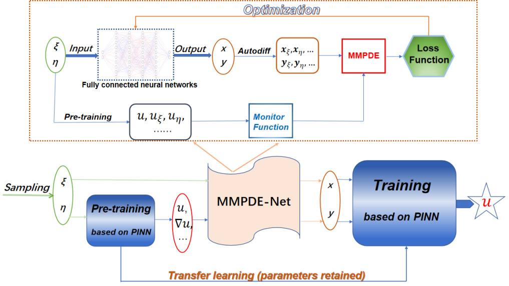
Figure 8: Flow chart of MS-PINN.

MS-PINN is described in Algorithm 3 for the two-dimensional problem, and the corresponding flowchart is given in Fig 8. In fact, the iterative algorithm in Section 3.2 can be applied to MS-PINN as well, by simply changing the single MMPDE-Net training in Algorithm 3 to multiple iterations of MMPDE-Net training (like Algorithm 2). We will not discuss further about this part, more details can be found in the numerical examples in Section 5.2.2.

4.2 Error Estimation

In this section, we will discuss the error estimate to verify the MS-PINN. We consider the problem Eq (1) and assume that both $\mathcal{A}$ and $\mathcal{B}$ are linear operators. According to the description in Section 3.1, traditional PINN usually samples collocation points based on a uniform distribution $U(\bm{x})$, and the collocation points output by MMPDE-Net are subject to a new distribution, denoted by $\rho_{MM}(\bm{x})$. In order to derive the error estimation for deep learning solvers, Assumption 2 for MMPDE-Net is given.

Assumption 2.

The optimization algorithm always finds the optimal parameters $\theta$ to minimize the loss function, i.e., $\min\limits_{\theta}\mathcal{L}oss_{MMPDE}(\xi,\eta;\theta)$.

Since the sampling distribution is very important, we define the norm $\|\cdot\|_{2,\rho}$ as follows

$$\|f(\bm{x})\|_{2,\rho}=\left(\int_{\Omega}|f(\bm{x})|^{2}\rho(\bm{x})d\bm{x}\right)^{\frac{1}{2}},\quad\bm{x}\in\Omega,$$ (18)

where $f(\bm{x})\in L^{2}(\Omega)$, $\rho(\bm{x})$ is a PDF. We now consider the PINN loss function as follows

$$\left\{\begin{aligned} &\mathcal{L}(\bm{x};\theta)=\alpha_{1}\mathcal{L}_{res}(\bm{x};\theta)+\alpha_{2}\mathcal{L}_{bou}(\bm{x};\theta),\\ &\mathcal{L}_{res}(\bm{x};\theta)=\|r(\bm{x};\theta)\|_{2,\rho,\Omega}^{2}=\int_{\Omega}|r(\bm{x};\theta)|^{2}\rho(\bm{x})d\bm{x},\quad\bm{x}\in\Omega,\\ &\mathcal{L}_{bou}(\bm{x};\theta)=\|b(\bm{x};\theta)\|_{2,\rho,\partial\Omega}^{2}=\int_{\partial\Omega}|b(\bm{x};\theta)|^{2}\rho(\bm{x})d\bm{x},\quad\bm{x}\in\partial\Omega.\\ \end{aligned}\right.$$ (19)

Without loss of generality, in all subsequent derivations, we choose $\alpha_{1}=\alpha_{2}=1$. We use Monte Carlo method to approximate the residual loss term $\mathcal{L}_{res}(\bm{x};\theta)$, which is

$$\mathcal{L}_{res}(\bm{x};\theta)=\int_{\Omega}|r(\bm{x};\theta)|^{2}\rho(\bm{x})d\bm{x}=\mathbb{E}_{\bm{x}\sim\rho}\left[|r(\bm{x};\theta)|^{2}\right]\approx\frac{1}{M_{r}}\sum_{i=1}^{M_{r}}|r(\bm{x}_{i};\theta)|^{2},\quad\bm{x}\sim\rho(\bm{x}).$$ (20)

The discrete form of the $\|\cdot\|_{2,\rho}$ norm is defined as

$$\|r(\bm{x};\theta)\|_{2,\rho,M_{r}}^{2}=\frac{1}{M_{r}}\sum_{i=1}^{M_{r}}|r(\bm{x}_{i};\theta)|^{2},\quad\bm{x}\sim\rho(\bm{x}).$$ (21)

Now we will prove that $\|r(\bm{x};\theta)\|_{2,\rho_{MM},M_{r}}^{2}\leq\|r(\bm{x};\theta)\|_{2,U,M_{r}}^{2}$. Without loss of generality, we divide the computational domain $\Omega$ into two parts based on the complexity of the function, i.e., $\Omega=\Omega_{1}+\Omega_{2}$, $k_{1}<k_{2}$, which denote the complexity of $\Omega_{1}$ and $\Omega_{2}$ respectively. We suppose $|\Omega_{1}|=\int_{\Omega_{1}}d\bm{x}>|\Omega_{2}|=\int_{\Omega_{2}}d\bm{x}$ and $M_{r}$ is the total number of sampling points in $\Omega$. If the sampling points are chosen from the uniform distribution, the numbers of sampling points in $\Omega_{1}$ and $\Omega_{2}$ are $\frac{b_{1}}{2}M_{r}$ and $\frac{b_{2}}{2}M_{r}\in\mathbb{N^{+}}$ respectively, where $b_{1}+b_{2}=2$. After training by MMPDE-Net, the number of sampling points in the two subregions changes to $\frac{a_{1}}{2}M_{r}$ and $\frac{a_{2}}{2}M_{r}\in\mathbb{N^{+}}$, respectively, where $a_{1}+a_{2}=2$.

Theorem 1.

Suppose that there exists $\hat{\theta}$ such that $\|r(\bm{x};\hat{\theta})\|_{2,\rho_{MM},M_{r}}^{2}=\mathbb{E}_{\theta}\left[\|r(\bm{x};\theta)\|_{2,\rho_{MM},M_{r}}^{2}\right]$, under Assumption 1 and 2, we have

$$\|r(\bm{x};\hat{\theta})\|_{2,\rho_{MM},M_{r}}^{2}\leq\|r(\bm{x};\hat{\theta})\|_{2,U,M_{r}}^{2}.$$

Proof.

Using Definition 1 and Assumption 1, it is obtained that

$$\|r(\bm{x};\hat{\theta})\|_{2,U,M_{r}}^{2} =\mathcal{F}\left(k_{1},\frac{b_{1}}{2}M_{r},M_{r}\right)+\mathcal{F}\left(k_{2},\frac{b_{2}}{2}M_{r},M_{r}\right)$$ (22)

$$=\frac{1}{b_{1}^{q}}\left(\frac{k_{1}}{k_{2}}\right)^{p}\mathcal{F}\left(k_{2},\frac{1}{2}M_{r},M_{r}\right)+\frac{1}{b_{2}^{q}}\mathcal{F}\left(k_{2},\frac{1}{2}M_{r},M_{r}\right)$$

$$=\left[\frac{1}{b_{1}^{q}}\left(\frac{k_{1}}{k_{2}}\right)^{p}+\frac{1}{b_{2}^{q}}\right]\mathcal{F}\left(k_{2},\frac{1}{2}M_{r},M_{r}\right).$$

$$\|r(\bm{x};\hat{\theta})\|_{2,\rho_{MM},M_{r}}^{2} =\mathcal{F}\left(k_{1},\frac{a_{1}}{2}M_{r},M_{r}\right)+\mathcal{F}\left(k_{2},\frac{a_{2}}{2}M_{r},M_{r}\right)$$ (23)

$$=\frac{1}{a_{1}^{q}}\left(\frac{k_{1}}{k_{2}}\right)^{p}\mathcal{F}\left(k_{2},\frac{1}{2}M_{r},M_{r}\right)+\frac{1}{a_{2}^{q}}\mathcal{F}\left(k_{2},\frac{1}{2}M_{r},M_{r}\right)$$

$$=\left[\frac{1}{a_{1}^{q}}\left(\frac{k_{1}}{k_{2}}\right)^{p}+\frac{1}{a_{2}^{q}}\right]\mathcal{F}\left(k_{2},\frac{1}{2}M_{r},M_{r}\right).$$

Since $\mathcal{F}\left(k_{2},\frac{1}{2}M_{r},M_{r}\right)>0$, it is only necessary to prove that

$$\frac{1}{a_{1}^{q}}\left(\frac{k_{1}}{k_{2}}\right)^{p}+\frac{1}{a_{2}^{q}}\leq\frac{1}{b_{1}^{q}}\left(\frac{k_{1}}{k_{2}}\right)^{p}+\frac{1}{b_{2}^{q}}.$$ (24)

Since $|\Omega_{1}|>|\Omega_{2}|$, we have $0<b_{2}<1<b_{1}<2$. As we described in Section 3.1, the points output by MMPDE-Net will be concentrated in $\Omega_{2}$, due to $k_{2}>k_{1}$. Therefore, we claim $0<a_{1}<b_{1}<2,\ 0<b_{2}<a_{2}<2$. Then, Eq (24) can be written as

$$\frac{1}{a_{1}^{q}}\left(\frac{k_{1}}{k_{2}}\right)^{p}+\frac{1}{a_{2}^{q}}\leq\frac{1}{b_{1}^{q}}\left(\frac{k_{1}}{k_{2}}\right)^{p}+\frac{1}{b_{2}^{q}}\iff \frac{a_{1}^{q}\left(\frac{a_{2}^{q}}{b_{2}^{q}}-1\right)}{a_{2}^{q}\left(1-\frac{a_{1}^{q}}{b_{1}^{q}}\right)}\geq\left(\frac{k_{1}}{k_{2}}\right)^{p}.$$ (25)

We take $a_{1}$ as the independent variable and introduce a continuous function $h(x)$ on $(0,b_{1})$

$$h(x)=\frac{x^{q}\left(\frac{(2-x)^{q}}{b_{2}^{q}}-1\right)}{\left(2-x\right)^{q}\left(1-\frac{x^{q}}{b_{1}^{q}}\right)}.$$ (26)

We have

$$\left\{\begin{aligned} h^{\prime}(x)&\geq 0,\\ \lim\limits_{x\rightarrow 0}h(x)&=0,\\ \lim\limits_{x\rightarrow b_{1}}h(x)&=\left(\frac{b_{1}}{b_{2}}\right)^{q}.\\ \end{aligned}\right.$$ (27)

Thus, $\exists\ x^{*}\in(0,b_{1})$, s.t. $h(x^{*})\geq\left(\frac{k_{1}}{k_{2}}\right)^{q}$, since $\left(\frac{b_{1}}{b_{2}}\right)^{q}>1>\left(\frac{k_{1}}{k_{2}}\right)^{q}$. Using Assumption 2 and the description in Section 3.2, choosing an appropriate monitor function and iterative process, the sampling points can be arbitrarily concentrated in $\Omega_{2}$, that is, the sampling points can be arbitrarily sparse in $\Omega_{1}$. Therefore, $a_{1}$ and $a_{2}$ satisfying Eq (24) can be found by our algorithm.

∎

Since $\mathcal{A}$ and $\mathcal{B}$ in Eq (1) are supposed to be linear operators, similar as in [24], the following assumption is given, which is the stability bound.

Assumption 3.

Let $\mathbb{H}$ be a Hilbert space, the following assumption holds

$$C_{1}\|\bm{u}\|_{2,\rho}\leq\|\mathcal{A}(\bm{u})\|_{2,\rho,\Omega}+\|\mathcal{B}(\bm{u})\|_{2,\rho,\partial\Omega}\leq C_{2}\|\bm{u}\|_{2,\rho},\ \forall\bm{u}\in\mathbb{H},$$ (28)

where $C_{1}$ and $C_{2}$ are positive constants.

In order to give an upper bound of the error, we need to introduce the the Rademacher complexity.

Definition 2.

Let $X:=\{x_{i}\}_{i=1}^{n}$ be a collection of i.i.d. random samples, the Rademacher complexity of the function class $\mathcal{F}$ can be defined as

$$\mathcal{R}_{n}(\mathcal{F})=\mathbb{E}_{X,\epsilon}\left(\sup_{f\in\mathcal{F}}|\frac{1}{n}\sum_{i=1}^{n}\epsilon_{i}f(x_{i})|\right),$$

where $(\epsilon_{1},\epsilon_{2},...,\epsilon_{n})$ are i.i.d. Rademacher variables, i.e., $P(\epsilon_{i}=1)=P(\epsilon_{i}=-1)=0.5$.

Let $\bm{u}^{*}$ be the exact solution of Eq (1), same as in [21], it is reasonable to assume that

Assumption 4.

There exists a positive number $0<b\in\mathbb{R}$ such that

$$\sup_{i}\|\mathcal{A}[\bm{u}_{i}(\bm{x})]-f(x)\|_{\infty}=b$$ (29)

where $\left\{\bm{u}_{i}(\bm{x})\right\}_{i\geq 1}\subset\mathbb{H}$ is a sequence of approximate solutions , i.e., $\lim\limits_{i\to+\infty}\|\bm{u}_{i}(\bm{x})-\bm{u}^{*}(\bm{x})\|_{2,\rho_{MM}}=0$.

Now we consider the approximate solution of the neural networks $\mathcal{F}^{NN}_{u}=\left\{\bm{u}(\bm{x};\theta):\theta\in\mathbb{R}^{NN}\right\}$. Similarly as in [21], using Assumption 4 and the Universal Approximation Theorem ([6],[7]), the following function class can be defined

$$\mathcal{F}_{r}=\left\{\bm{u}(\bm{x};\theta):\bm{u}(\bm{x};\theta)\in\mathbb{H}\cap\mathcal{F}^{NN}_{u}\ \mbox{and}\ \|\mathcal{A}[\bm{u}(\bm{x};\theta)]-f(\bm{x})\|_{\infty,\Omega}\leq b\right\},$$

which is not empty.

According to [25], we use Lemma 1 and propose the following theorem about the Rademacher complexity.

Lemma 1.

Let $\mathcal{F}$ be a b-uniformly bounded class of integrable real-valued functions with domain $\Omega$, for any postive integer $n\geq 1$ and any scalar $\delta\geq 0$, we have

$$\sup_{f\in\mathcal{F}}\left|\frac{1}{n}\sum_{i=1}^{n}f(x_{i})-\mathbb{E}[f(x)]\right|\leq 2\mathcal{R}_{n}(\mathcal{F})+\delta,$$

with probability at least $1-exp\left(-\frac{n\delta^{2}}{2b^{2}}\right)$.

Theorem 2.

Suppose that Assumption 3 and Assumption 4 hold, let $\bm{u}^{*}$ be the exact solution of Eq (1). Given $\delta>0$, $\{x_{i}\}_{i=1}^{M_{r}}$ is a collection of i.i.d. random samples from the PDF $\rho_{MM}$ and $\forall\bm{u}(\bm{x};\theta)\in\mathcal{F}_{r}$, the following error estimate holds

$$\|\bm{u}^{*}(\bm{x})-\bm{u}(\bm{x};\theta)\|_{2,\rho_{MM}}\leq\frac{\sqrt{2}}{C_{1}}\left(\|r(\bm{x};\theta)\|_{2,\rho_{MM},M_{r}}^{2}+\|b(\bm{x};\theta)\|_{2,\rho_{MM},\partial\Omega}^{2}+2\mathcal{R}_{M_{r}}(\mathcal{F}_{r})+\delta\right)^{\frac{1}{2}},$$ (30)

with probability at least $1-\exp\left(-\frac{M_{r}\delta^{2}}{2b^{2}}\right)$.

Proof.

By Assumption 3, we have

$$C_{1}\|\bm{u}^{*}(\bm{x})-\bm{u}(\bm{x};\theta)\|_{2,\rho_{MM}} \leq\|\mathcal{A}(\bm{u}^{*}(\bm{x}))-\mathcal{A}(\bm{u}(\bm{x};\theta))\|_{2,\rho_{MM},\Omega}+\|\mathcal{B}(\bm{u}^{*}(\bm{x}))-\mathcal{B}(\bm{u}(\bm{x};\theta))\|_{2,\rho_{MM},\partial\Omega}$$ (31)

$$=\|\mathcal{A}(\bm{u}(\bm{x};\theta))-f\|_{2,\rho_{MM},\Omega}+\|\mathcal{B}(\bm{u}(\bm{x};\theta))-g\|_{2,\rho_{MM},\partial\Omega}$$

$$=\|r(\bm{x};\theta)\|_{2,\rho_{MM},\Omega}+\|b(\bm{x};\theta)\|_{2,\rho_{MM},\partial\Omega}$$

$$\leq\sqrt{2}\left(\|r(\bm{x};\theta)\|_{2,\rho_{MM},\Omega}^{2}+\|b(\bm{x};\theta)\|_{2,\rho_{MM},\partial\Omega}^{2}\right)^{\frac{1}{2}}.$$

Using Lemma 1, we have

$$\|r(\bm{x};\theta)\|_{2,\rho_{MM},\Omega}^{2}\leq\|r(\bm{x};\theta)\|_{2,\rho_{MM},M_{r}}^{2}+2\mathcal{R}_{M_{r}}(\mathcal{F}_{r})+\delta,$$ (32)

with probability at least $1-\exp\left(-\frac{M_{r}\delta^{2}}{2b^{2}}\right)$. Therefore,

$$\|\bm{u}^{*}(\bm{x})-\bm{u}(\bm{x};\theta)\|_{2,\rho_{MM}} \leq\frac{\sqrt{2}}{C_{1}}(\|r(\bm{x};\theta)\|_{2,\rho_{MM},\Omega}^{2}+\|b(\bm{x};\theta)\|_{2,\rho_{MM},\partial\Omega}^{2})^{\frac{1}{2}}$$ (33)

$$\leq\frac{\sqrt{2}}{C_{1}}\left(\|r(\bm{x};\theta)\|_{2,\rho_{MM},M_{r}}^{2}+\|b(\bm{x};\theta)\|_{2,\rho_{MM},\partial\Omega}^{2}+2\mathcal{R}_{M_{r}}(\mathcal{F}_{r})+\delta\right)^{\frac{1}{2}},$$

with probability at least $1-\exp\left(-\frac{M_{r}\delta^{2}}{2b^{2}}\right)$. ∎

Corollary 1.

Suppose that Theorem 1 and Theorem 2 hold, then

$$\|\bm{u}^{*}(\bm{x})-\bm{u}(\bm{x};\hat{\theta})\|_{2,\rho_{MM}} \leq\frac{\sqrt{2}}{C_{1}}\left(\|r(\bm{x};\hat{\theta})\|_{2,\rho_{MM},M_{r}}^{2}+\|b(\bm{x};\hat{\theta})\|_{2,\rho_{MM},\partial\Omega}^{2}+2\mathcal{R}_{M_{r}}(\mathcal{F}_{r})+\delta\right)^{\frac{1}{2}}$$ (34)

$$\leq\frac{\sqrt{2}}{C_{1}}\left(\|r(\bm{x};\hat{\theta})\|_{2,U,M_{r}}^{2}+\|b(\bm{x};\hat{\theta})\|_{2,U,\partial\Omega}^{2}+2\mathcal{R}_{M_{r}}(\mathcal{F}_{r})+\delta\right)^{\frac{1}{2}},$$

with probability at least $1-\exp\left(-\frac{M_{r}\delta^{2}}{2b^{2}}\right)$.

Proof.

By Theorem 1, we have

$$\|r(\bm{x};\hat{\theta})\|_{2,\rho_{MM},M_{r}}^{2}\leq\|r(\bm{x};\hat{\theta})\|_{2,U,M_{r}}^{2}.$$ (35)

Since only the distribution of points within $\Omega$ varies after training by MMPDE-Net and the distribution of points on $\partial\Omega$ is unchanged, we have

$$\|b(\bm{x};\hat{\theta})\|_{2,\rho_{MM},\partial\Omega}^{2}=\|b(\bm{x};\hat{\theta})\|_{2,U,\partial\Omega}^{2}.$$ (36)

Therefore,

$$\|\bm{u}^{*}(\bm{x})-\bm{u}(\bm{x};\hat{\theta})\|_{2,\rho_{MM}} \leq\frac{\sqrt{2}}{C_{1}}\left(\|r(\bm{x};\hat{\theta})\|_{2,\rho_{MM},M_{r}}^{2}+\|b(\bm{x};\hat{\theta})\|_{2,\rho_{MM},\partial\Omega}^{2}+2\mathcal{R}_{M_{r}}(\mathcal{F}_{r})+\delta\right)^{\frac{1}{2}}$$

$$\leq\frac{\sqrt{2}}{C_{1}}\left(\|r(\bm{x};\hat{\theta})\|_{2,U,M_{r}}^{2}+\|b(\bm{x};\hat{\theta})\|_{2,U,\partial\Omega}^{2}+2\mathcal{R}_{M_{r}}(\mathcal{F}_{r})+\delta\right)^{\frac{1}{2}},$$

with probability at least $1-\exp\left(-\frac{M_{r}\delta^{2}}{2b^{2}}\right)$. ∎

It is observed from Corollary 1 that the upper bound of the error in $\|\cdot\|_{2,\rho_{MM}}$ can be reduced by MMPDE-Net.

5 Numerical Experiments

In this section, numerical experiments are presented to verify our method. A two-dimensional Poisson equation with low regularity, which has one peak is discussed in Section 5.2. We compare our method with other methods and show the performance of MS-PINN with iterative MMPDE-Net. In Section 5.3, numerical solutions of two-dimensional Poisson equation with two peaks are presented. Numerical results in Section 5.4 show that our algorithm is effective for solving Burgers equation, whose solution has large gradient, including both forward (Section5.4.1) and inverse (Section 5.4.2) problems. The last example in Section 5.5 is the two-dimensional Burgers problem, which has shock wave solution in finite time.

5.1 Symbols and parameter settings

The analytical solution or reference solution is denoted by $u^{*}$. The $u^{\text{PINN}}$ and $u^{\text{MS-PINN}}$ are used to denote the approximate solutions obtained by PINN and MSPINN respectively. According to Eq (21), the relative errors in the test set $\left\{\bm{x}_{i}\right\}_{i=1}^{M_{t}}$ sampled from the equispaced uniform distribution are defined as follows

$$\begin{array}[]{r@{}l}\begin{aligned} e_{\infty}(u)&=\frac{\|u^{*}-u\|_{\infty,U,M_{t}}}{\|u^{*}\|_{\infty,U,M_{t}}},\\ e_{2}(u)&=\frac{\|u^{*}-u\|_{2,U,M_{t}}}{\|u^{*}\|_{2,U,M_{t}}}.\end{aligned}\end{array}$$ (37)

Parameter settings in MS-PINN are given in Table 2 if we do not specify otherwise. For Poisson equation and forward Burgers equation, the Adam method is used to do the optimization. For the inverse Burgers equation and two dimensional Poisson equation, the Adam method is implemented firstly and then the LBFGS method is used to optimize the loss function. Since there is three stages in MS-PINN, we have given the training epochs in two stages in Table 2, while the training epochs in MMPDE-Net is specified in each case. All simulations are carried on NVIDIA A100(80G).

Table 2: Default settings for main parameters in MS-PINN.

Torch	Activation	Initialization	Optimization	Learning	Eq (17)
Version	Function	Method	Method	Rate	$\tau$
2.0.1	tanh	Xavier	Adam/LBFGS	0.0001/1	0.1
MMPDE-Net	Poisson	Burgers	MMPDE-Net	Pre-	Formal
Size	PINN Size	PINN Size	Training	Training	Training
(neurons/layer	(neurons/layer	(neurons/layer	(epochs)	(epochs)	(epochs)
$\times$ hidden layers)	$\times$ hidden layers)	$\times$ hidden layers)
$20\times 8$	$40\times 4$	$20\times 8$	20000	20000	40000

5.2 Two-dimensional Poisson equation with one peak

For the following two-dimensional Poisson equation

$$\begin{array}[]{r@{}l}\left\{\begin{aligned} -\Delta u(x,y)&=f(x,y),\quad(x,y)\ \mbox{in}\ \Omega,\\ u(x,y)&=g(x,y),\quad(x,y)\ \mbox{on}\ \partial\Omega,\end{aligned}\right.\end{array}$$ (38)

where $\Omega=(-1,1)^{2}$, the analytical solution with one peak at $(0,0)$ is chosen as

$$\begin{array}[]{r@{}l}\begin{aligned} u=e^{-1000(x^{2}+y^{2})}.\end{aligned}\end{array}$$ (39)

The Dirichlet boundary condition $g(x,y)$ on $\partial\Omega$ and function $f(x,y)$ are given by the analytical solution.

5.2.1 MS-PINN

As shown in Fig 8, we firstly use PINN for pre-training to obtain the preliminary solution information, secondly input it into MMPDE-Net together with the training points, finally input the new training points obtained from the second stage into PINN for the formal training. The monitor function in MMPDE-Net for Eq (38) is chosen as

$$\begin{array}[]{r@{}l}\begin{aligned} w=\sqrt{1+1000u^{2}+\lvert\nabla u\rvert^{2}}.\end{aligned}\end{array}$$ (40)

In order to compare our method with other three methods, we sample $100\times 100$ points in $\Omega$ and 300 points on $\partial\Omega$ as the training set and $400\times 400$ points as the test set for all the methods. In MS-PINN, we train MMPDE-Net 20000 epochs, and the epochs of pre-training formal PINN training are shown in Table 2. Four different methods are implemented: (1) PINN that samples $100\times 100$ uniformly distributed points and trains 60000 epochs; (2) PINN-RAR method that pre-trains 20000 epochs using $90\times 90$ training points, then 1900 more training points are added by RAR method ([13],[27]) and trains 40000 epochs; (3) PINN-RAD method that pre-trains 20000 epochs using $100\times 100$ training points, then 10000 points were adaptively sampled by RAD method ([27],[15],[30]) and trains 40000 epochs.

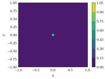
(a) analytical solution

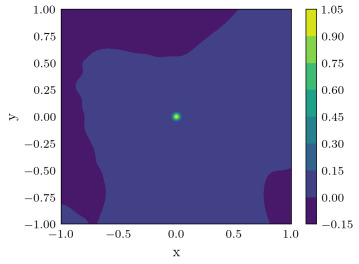
(b) approximate solution

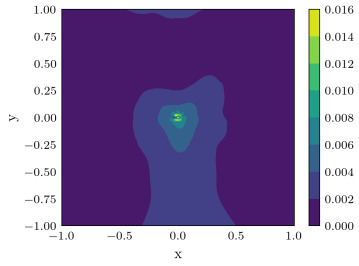
(c) absolute error

Figure 9: The result of PINN for the two-dimensional Poisson equation with one peak. (a) the analytical solution $u^{*}$ of the equation; (b) the approximate solution $u^{\text{PINN}}$ of PINN; (c) the absolute error $|u^{*}-u^{\text{PINN}}|$.

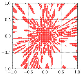
(a) training points added by RAR

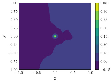
(b) approximate solution

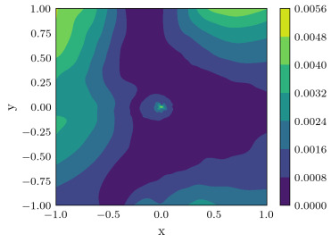
(c) absolute error

Figure 10: The result of PINN-RAR for the two-dimensional Poisson equation with one peak. (a) training points added by RAR method; (b) the approximate solution $u^{\text{PINN-RAR}}$; (c) the absolute error $|u^{*}-u^{\text{PINN-RAR}}|$.

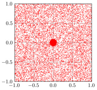
(a) training points added by RAD

(b) approximate solution

(c) absolute error

Figure 11: The result of PINN-RAD for the two-dimensional Poisson equation with one peak. (a) training points sampled by RAD method (k=1,c=1); (b) the approximate solution $u^{\text{PINN-RAD}}$; (c) the absolute error $|u^{*}-u^{\text{PINN-RAD}}|$.

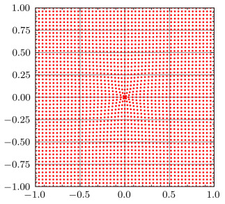
(a) new distribution of sampling points

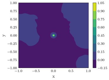
(b) approximate solution

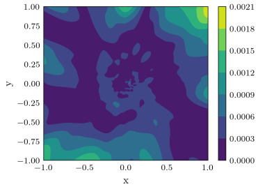
(c) absolute error

Figure 12: The result of MS-PINN for the two-dimensional Poisson equation with one peak. (a) new training points output by MMPDE-Net, for ease of viewing, we only show $50\times 50$ points; (b) the approximate solution $u^{\text{MS-PINN}}$ of the MS-PINN; (c) the absolute error $|u^{*}-u^{\text{MS-PINN}}|$.

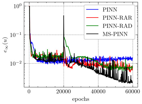
(a) performance of $e_{\infty}(u)$ during training

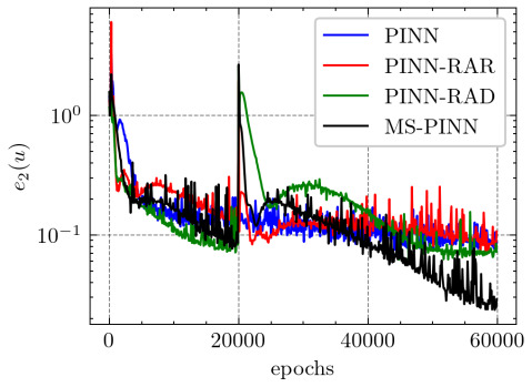
(b) performance of $e_{2}(u)$ during training

Figure 13: (a) the performance of relative error $e_{\infty}(u)$ with different training epochs, (b) the performance of relative error $e_{2}(u)$ with different training epochs.

The numerical results of PINN are given in Fig 9. The distribution of the training points added by RAR method and the approximation solution of PINN-RAR are shown in Fig 10. The distribution of the training points sampled by RAD method and the approximation solution of PINN-RAD are shown in Fig 11. The distribution of the training points generated by MMPDE-Net and the approximation solution of MS-PINN are shown in Fig 12. The performance of the four different methods in terms of relative errors at the training points during the training process is given by Fig 13. It is observed that there is a big jump of errors at epoch $=20000$ in Fig 13, which is due to that pre-training with PINN works in the first stage, MMPDE-Net takes effect after epoch $=20000$ and points are redistributed meanwhile. Similar phenomena arise in other cases. Moreover, a comparison of errors using different methods is given in Table 3. From these results, it is observed that MS-PINN can obtain better results than the other methods.

Table 3: Comparison of errors using different methods.

Relative	$100\times 100$	$100\times 100$	$100\times 100$	$100\times 100$
error	PINN	PINN-RAR	PINN-RAD	MS-PINN
$e_{\infty}(u)$	$1.593\times 10^{-2}$	$4.916\times 10^{-3}$	$6.062\times 10^{-3}$	$2.038\times 10^{-3}$
$e_{2}(u)$	$8.844\times 10^{-2}$	$8.879\times 10^{-2}$	$8.927\times 10^{-2}$	$2.686\times 10^{-2}$

5.2.2 MS-PINN with the iterative MMPDE-Net

For Eq (38), we implement MS-PINN with iterative MMPDE-Net (Algorithm 2). The monitor function that we use is

$$\begin{array}[]{r@{}l}\begin{aligned} w=1+2u.\end{aligned}\end{array}$$ (41)

We sample $80\times 80$ points in $\Omega$ and 324 points on $\partial\Omega$ as the training set and $400\times 400$ points as the test set. Four experiments with different training strategies are used to validate the effectiveness of the iterative MMPDE-Net method: PINN, MS-PINN with one MMPDE-Net iteration, MS-PINN with three MMPDE-Net iterations and MS-PINN with five MMPDE-Net iterations (See Table 4).

Table 4: Settings of four training strategies.

Training	Sampling	USE	MMPDE-Net	MMPDE-Net	Pre-training	Formal training
strategy	points	MMPDE-Net	iterations	epochs	epochs	epochs
Strategy 1	6400+324	No	-	-	-	70000
Strategy 2	6400+324	Yes	1	20000	20000	50000
Strategy 3	6400+324	Yes	3	60000	20000	50000
Strategy 4	6400+324	Yes	5	100000	20000	50000

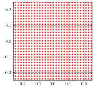
(a) initial training points

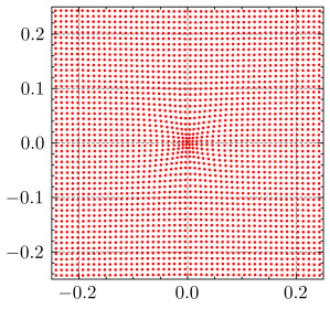
(b) after 1 iteration

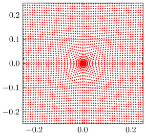
(c) after 3 iterations

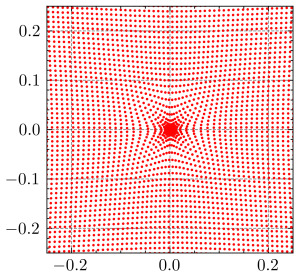
(d) after 5 iterations

Figure 14: The results of iterative MMPDE-Net for the two-dimensional Poisson equation with one peak. To see the results clearly, we show the region $[-0.25,0.25]^{2}$ particularly.

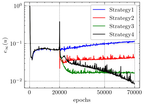
(a) performance of $e_{\infty}(u)$ during training

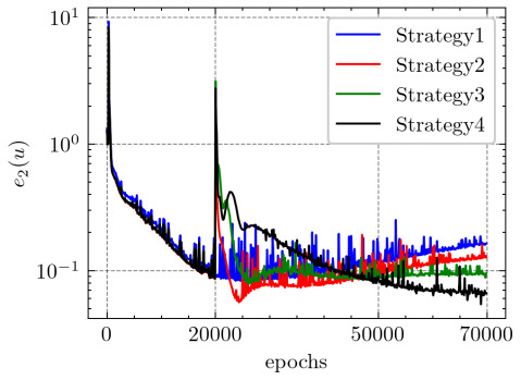
(b) performance of $e_{2}(u)$ during training

Figure 15: (a) the performance of relative error $e_{\infty}(u)$ with different training epochs; (b) the performance of relative error $e_{2}(u)$ with different training epochs.

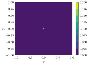
(a) PINN

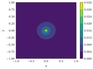
(b) after 1 iteration

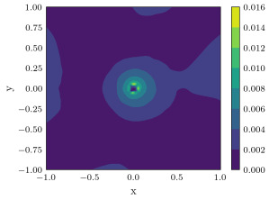
(c) after 3 iterations

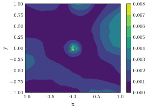
(d) after 5 iterations

Figure 16: The absolute errors of MS-PINN using iterative MMPDE-Net for the two-dimensional Poisson equation with one peak. (a) the absolute error of PINN; (b) the absolute error of MS-PINN using MMPDE-Net with one iteration; (c) the absolute error of MS-PINN using MMPDE-Net with three iterations; (d) the absolute error of MS-PINN using MMPDE-Net with five iterations.

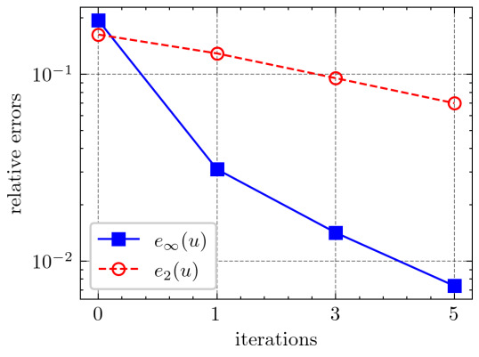
Figure 17: The relative errors of MS-PINN with different MMPDE-Net iterations.

From Fig 14, it can be seen that the sampling points obtained from MMPDE-Net are concentrated much more on the place where the solution has large variations as the number of iterations increases. The performance of the four different strategies in terms of relative errors during the training process is given in Fig 15. MMPDE-Net iteration can reduce the errors effectively, since it make the points move to the places where need more samplings. From Fig 16 and Fig 17, it can be seen that MMPDE-Net with iterations in MS-PINN can improve the numerical results, the relative errors decrease as the number of iterations increases.

5.3 Two-dimensional Poisson equation with two peaks

Consider the two-dimensional Poisson equation Eq (38) in $\Omega=(-1,1)^{2}$, the analytical solution with two peaks is given by

$$\begin{array}[]{r@{}l}\begin{aligned} u=e^{-1000\left(x^{2}+(y-0.5)^{2}\right)}+e^{-1000\left(x^{2}+(y+0.5)^{2}\right)}.\end{aligned}\end{array}$$ (42)

The monitor function that we use in MMPDE-Net is

$$\begin{array}[]{r@{}l}\begin{aligned} w=\sqrt{1+1000u^{2}+\lvert\nabla u\rvert^{2}}.\end{aligned}\end{array}$$ (43)

We sample $100\times 100$ points in $\Omega$ and 400 points on $\partial\Omega$ as the training set and $400\times 400$ points as the test set. The setting of main parameters in MS-PINN is given in Table 2. We compare the numerical results of MS-PINN with the results obtained by PINN trained 60000 epochs to show the effectiveness of our method.

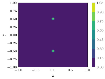
(a) analytical solution

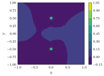
(b) approximate solution

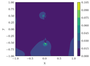
(c) absolute error

Figure 18: The result of PINN for the two-dimensional Poisson equation with two peaks. (a) the analytical solution $u^{*}$ of the equation; (b) the approximate solution $u^{\text{PINN}}$ of PINN; (c) the absolute error $|u^{*}-u^{\text{PINN}}|$.

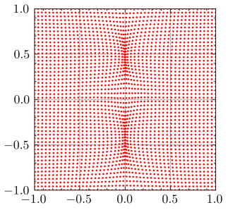
(a) new distribution of sampling points

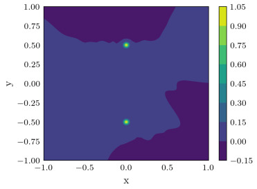
(b) approximate solution

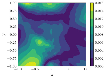
(c) absolute error

Figure 19: The results of MS-PINN for the two-dimensional Poisson equation with two peaks. (a) new training points obtained by MMPDE-Net; (b) the approximate solution $u^{\text{MS-PINN}}$ of the MS-PINN; (c) the absolute error $|u^{*}-u^{\text{MS-PINN}}|$.

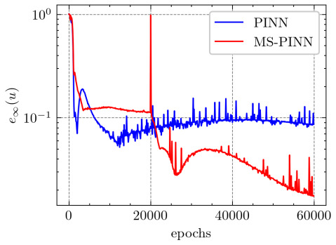
(a) performance of $e_{\infty}(u)$ during training

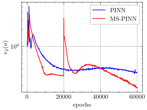
(b) performance of $e_{2}(u)$ during training

Figure 20: (a) the performance of relative error $e_{\infty}(u)$ with different training epochs; (b) the performance of relative error $e_{2}(u)$ with different training epochs.

The numerical results of PINN are given in Fig 18. The distribution of the training points generated by MMPDE-Net and the approximation solution of MS-PINN are shown in Fig 19. The performance of PINN and MS-PINN in terms of relative errors during the training process is given in Fig 20, which shows that MS-PINN behaves better than PINN.

5.4 One-dimensional Burgers equation

5.4.1 Forward problem

Consider the following one-dimensional Burgers equation [17]

$$\begin{array}[]{r@{}l}\left\{\begin{aligned} &u_{t}+uu_{x}-\frac{0.01}{\pi}u_{xx}=0,\quad x\in(-1,1),\quad t\in(0,1),\\ &u(x,0)=-\sin(\pi x),\quad x\in[-1,1],\\ &u(-1,t)=u(1,t)=0,\quad t\in[0,1],\\ \end{aligned}\right.\end{array}$$ (44)

the analytical solution is given in [1].

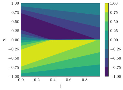
(a) $u^{\text{PINN}}$

(b) $u^{\text{MSPINN}}$

(c) $u^{*}$

Figure 21: The solutions of the forward problem for the one-dimensional Burgers equation. (a) the solution $u^{\text{PINN}}$ predicted by PINN; (b) the solution $u^{\text{MSPINN}}$ predicted by MSPINN; (c) the analytic solution $u^{*}$.

The monitor function that we use in MMPDE-Net is

$$\begin{array}[]{r@{}l}\begin{aligned} w=\sqrt{1+u^{2}+(0.5u_{x})^{2}}.\end{aligned}\end{array}$$ (45)

In $[-1,1]\times[0,1]$, we sample $152\times 100$ points as the training set and $256\times 100$ points as the test set. The settings of main parameters are in Table 2. We compare the numerical results of MS-PINN with the results obtained by PINN trained 60000 epochs to show the effectiveness of our method.

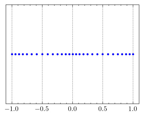
(a) new distribution of sampling points

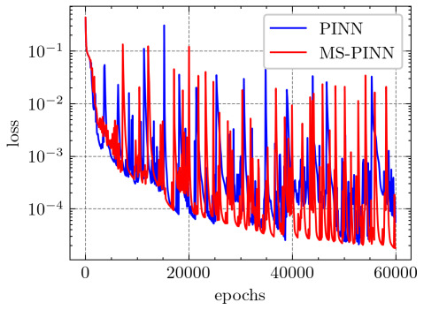
(b) performance of the loss function

Figure 22: (a) the distribution of new training points obtained by MMPDE-Net for forward Burgers equation (44); (b) the loss function with different training epochs.

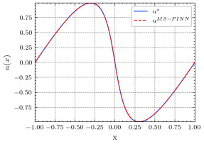
(a) t=0.2

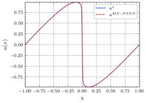
(b) t=0.4

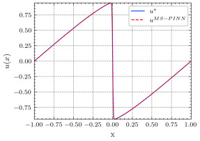
(c) t=0.6

(d) t=0.8

Figure 23: The results of MS-PINN at different times for the one-dimensional Burgers equation. (a) t=0.2; (b) t=0.4; (c) t=0.6; (d) t=0.8.

The solution $u^{\text{PINN}}$ predicted by PINN is shown in Fig 21(a). MMPDE-Net is implemented and the distribution of new training points is shown in Fig 22(a), where we only show 27 points for clear viewing. Fig 22(b) shows the variation of the loss function for PINN and MS-PINN with different training epochs, where it is noticed that MS-PINN can attain lower loss values. The solution $u^{\text{MSPINN}}$ predicted by MS-PINN is shown in Fig 21(b) and the analytical solution is shown in Fig 21(c). The comparison between the analytic solutions and the approximation solutions of MS-PINN at different time is shown in Fig 23. The relative errors at different time obtained by PINN and MS-PINN are presented in Fig 24, which again shows that our method can achieve more accurate results.

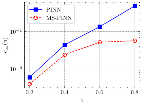
(a) $e_{\infty}(u)$

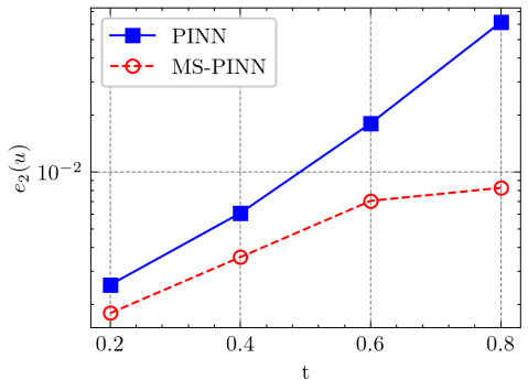
(b) $e_{2}(u)$

Figure 24: Comparison of the relative errors obtained by PINN and MS-PINN at different time.

5.4.2 Inverse problem

Consider the following one-dimensional Burgers equation [17]

$$\begin{array}[]{r@{}l}\left\{\begin{aligned} &u_{t}+\lambda_{1}uu_{x}-\lambda_{2}u_{xx}=0,\quad x\in(-1,1),\quad t\in(0,1),\\ &u(x,0)=-\sin(\pi x),\quad x\in[-1,1],\\ &u(-1,t)=u(1,t)=0,\quad t\in[0,1],\\ \end{aligned}\right.\end{array}$$ (46)

where $\lambda_{1}$ and $\lambda_{2}$ are the unknown parameters.

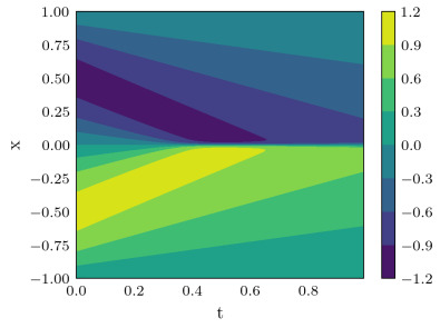
(a) $u^{\text{PINN}}$

(b) $u^{\text{MSPINN}}$

(c) $u^{*}$

Figure 25: The solutions of the inverse problem for the one-dimensional Burgers equation. (a) the solution $u^{\text{PINN}}$predicted by PINN; (b) the solution $u^{\text{MSPINN}}$ predicted by MSPINN ; (c) the analytic solution $u^{*}$.

The monitor function that we use in MMPDE-Net is

$$\begin{array}[]{r@{}l}\begin{aligned} w=\sqrt{1+(0.5u_{x})^{2}}.\end{aligned}\end{array}$$ (47)

In $[-1,1]\times[0,1]$, we sample $202\times 100$ points as the training set and $256\times 100$ points as the test set. In addition, the analytical solution corresponding to $\lambda_{1}^{*}=1$ and $\lambda_{2}^{*}=\frac{0.01}{\pi}$ is extracted for data-driven values at the uniformly sampled 200 points. The main setting parameters are shown in Table 2. For the MS-PINN, we train PINN 70000 epochs and MMPDE-Net 20000 epochs, where 20000 epochs in the pre-training of PINN and 50000 epochs in the formal PINN training. It is worth noting that the LBFGS method is used for fine-tuning in the last 10000 training epochs. We compare the numerical results of MS-PINN with the results obtained by PINN trained 70000 epochs to show the effectiveness of our method.

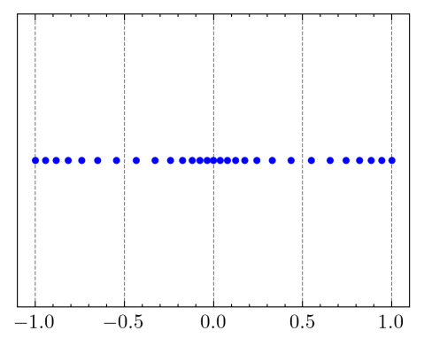
(a) new distribution of sampling points

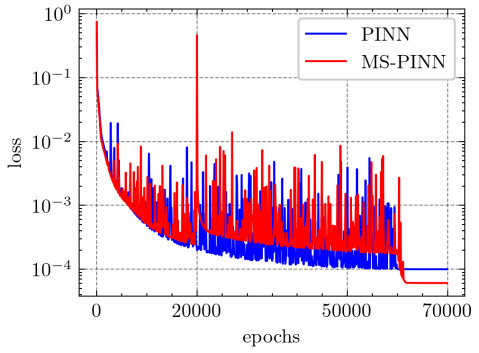
(b) performance of the loss function

Figure 26: (a) the distribution of new training points obtained by MMPDE-Net for inverse Burgers equation (46); (b) the performance of loss function with different training epochs.

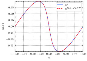
(a) t=0.2

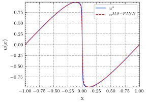
(b) t=0.4

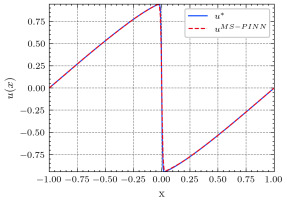
(c) t=0.6

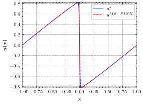
(d) t=0.8

Figure 27: The results of MS-PINN at different times for the one-dimensional inverse Burgers equation. (a) t=0.2; (b) t=0.4; (c) t=0.6; (d) t=0.8.

Table 5: Comparison of the absolute errors of PINN and MS-PINN on $\lambda_{1}$ and $\lambda_{2}$, where $\lambda^{\text{NN}}$ is denoted as the prediction of the neural networks.

absolute error	PINN	MS-PINN
$|\lambda_{1}^{\text{NN}}-\lambda_{1}^{*}|$	$2.932\times 10^{-3}$	$4.379\times 10^{-4}$
$|\lambda_{2}^{\text{NN}}-\lambda_{2}^{*}|$	$2.629\times 10^{-3}$	$1.427\times 10^{-3}$

The solution $u^{\text{PINN}}$ predicted by PINN is shown in Fig 25(a). MMPDE-Net is implemented and the distribution of new training points is shown in Fig 26(a), where we use only 27 points for clear viewing. Fig 26(b) shows the variation of the loss function for PINN and MS-PINN with different training epochs, where MS-PINN can attain lower loss values when using LBFGS to optimize. The solution $u^{\text{MSPINN}}$ predicted by MS-PINN is shown in Fig 25(b) and the analytical solution is shown in Fig 25(c) . The comparison between the analytic solutions and the approximation solutions of MS-PINN at different time is shown in Fig 27. The comparison of the absolute errors of $\lambda_{1}$ and $\lambda_{2}$ obtained by PINN and MS-PINN is shown in Table 5. The relative errors at different time obtained by PINN and MS-PINN are presented in Fig 28, which again demonstrates that our method can obtain more accurate results.

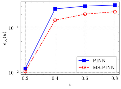
(a) $e_{\infty}(u)$

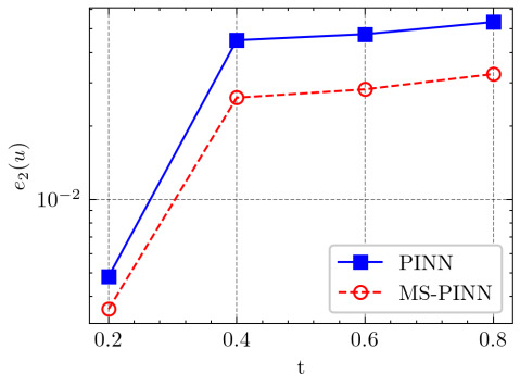
(b) $e_{2}(u)$

Figure 28: Comparison of the relative errors obtained by PINN and MS-PINN at different time.

5.5 Two-dimensional Burgers equation

Now consider the following two-dimensional Burgers equation [31]

$$\begin{array}[]{r@{}l}\left\{\begin{aligned} &u_{t}+uu_{x}+uu_{y}=0\quad(x,y)\in[0,4]^{2},\quad t\in[0,\frac{1.5}{\pi}],\\ &u(x,0,t)=u(x,4,t)\quad(x,t)\in[0,4]\times[0,\frac{1.5}{\pi}],\\ &u(0,y,t)=u(4,y,t)\quad(y,t)\in[0,4]\times[0,\frac{1.5}{\pi}],\\ &u(x,y,0)=\sin\left(\frac{\pi}{2}(x+y)\right),\quad(x,y)\in[0,4]^{2}.\\ \end{aligned}\right.\end{array}$$ (48)

The reference solutions at different time are given by method of characteristics and Newton’s method, which are shown in Fig 29(d). At $t=\frac{1}{\pi}$, there will be two shock waves on $x+y=2$ and $x+y=6$. The monitor function we use in MMPDE-Net is

$$\begin{array}[]{r@{}l}\begin{aligned} w=\sqrt{1+10u^{2}_{x}+10u^{2}_{y}}.\end{aligned}\end{array}$$ (49)

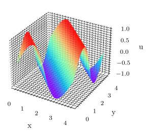
(a) $u^{\text{MSPINN}}$ at $t=\frac{0.375}{\pi}$

(b) $u^{*}$ at $t=\frac{0.375}{\pi}$

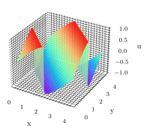
(c) $u^{\text{MSPINN}}$ at $t=\frac{1.5}{\pi}$

(d) $u^{*}$ at $t=\frac{1.5}{\pi}$

Figure 29: The solution predicted by MS-PINN and the reference solution for the two-dimensional Burgers equation at $t=\frac{0.375}{\pi}$ and $t=\frac{1.5}{\pi}$.

We sample $100\times 100\times 50$ points in $(0,4)^{2}\times[0,\frac{1.5}{\pi}]$ and 10000 on the boundary as the training set and $256\times 256\times 100$ points as the test set. The main setting parameters are shown in Table 2. For the MS-PINN, we train PINN 130000 epochs and MMPDE-Net 40000 epochs, where 20000 epochs in the pre-training of PINN and 110000 epochs in the formal PINN training. We compare the numerical results of MS-PINN with the results obtained by PINN which trained 130000 epochs to show the effectiveness of our method. It is worth noting that during the training of the PINN, we force the initial value condition and use the LBFGS method for fine-tuning in the last 30000 training epochs.

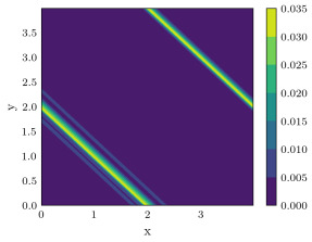
(a) $t=\frac{0.375}{\pi}$

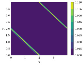
(b) $t=\frac{0.75}{\pi}$

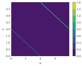
(c) $t=\frac{1.125}{\pi}$

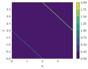
(d) $t=\frac{1.5}{\pi}$

Figure 30: The absolute errors approximated by PINN at different time for the two-dimensional Burgers equation. (a) $t=\frac{0.375}{\pi}$ (b) $t=\frac{0.75}{\pi}$ (c) $t=\frac{1.125}{\pi}$ (d) $t=\frac{1.5}{\pi}$ .

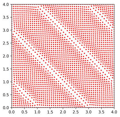
(a) new distribution of sampling points

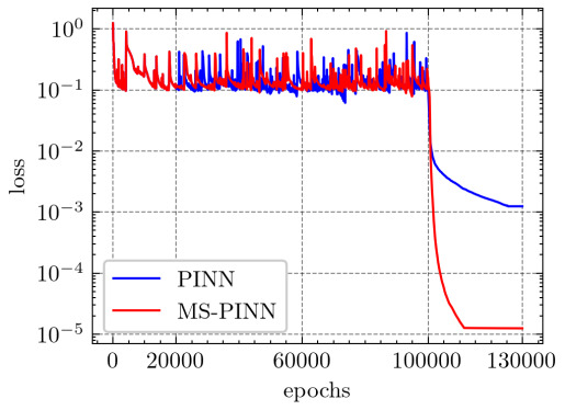
(b) performance of the loss function

Figure 31: (a) the distribution of new training points obtained by MMPDE-Net; (b) the loss function with different training epochs.

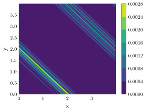
(a) $t=\frac{0.375}{\pi}$

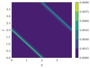
(b) $t=\frac{0.75}{\pi}$

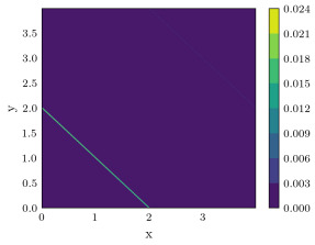
(c) $t=\frac{1.125}{\pi}$

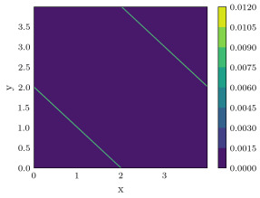
(d) $t=\frac{1.5}{\pi}$

Figure 32: The absolute errors approximated by MS-PINN at different time for the two-dimensional Burgers equation. (a) $t=\frac{0.375}{\pi}$ (b) $t=\frac{0.75}{\pi}$ (c) $t=\frac{1.125}{\pi}$ (d) $t=\frac{1.5}{\pi}$.

Fig 30 shows the absolute error approximated by PINN at different time. Fig 31(a) shows the output sampling points, which is performed at $t=0$ and we only show $50\times 50$ points for clear viewing. Fig 31(b) shows the variation of the loss function for PINN and MS-PINN with different training epochs, where MS-PINN can obtain much lower loss values. Fig 32 shows the absolute error approximated by MS-PINN at different time. For a more detailed view, the relative errors of the approximation solutions of PINN and MS-PINN at different time are shown in Fig 33. Our method can attain better results.

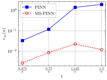
(a) $e_{\infty}(u)$

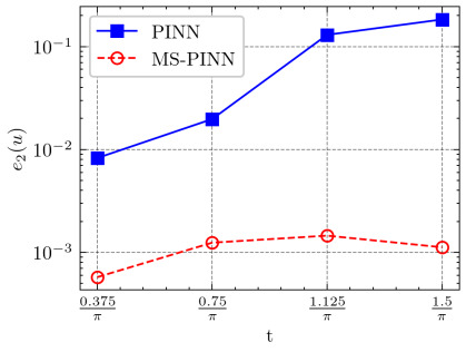
(b) $e_{2}(u)$

Figure 33: Comparison of the relative errors obtained by PINN and MS-PINN at different time.

6 Conclusions

In this work, unlike the usual sampling methods based on the loss function perspective, we propose the neural networks MMPDE-Net, which based on the moving mesh PDE method. It is an end-to-end, deep learning solver-independent framework which is designed to implement adaptive sampling. We also develop an iterative algorithm based on MMPDE-Net that is used to control the distribution of sampling points more precisely. The Moving Sampling PINN (MS-PINN) is proposed by combing MMPDE-Net and PINN. Some error estimates are given and sufficient numerical experiments are shown to demonstrate the effectiveness of our methods.

In the future, we will work on how to develop MMPDE-Net in the case of high-dimensional PDEs, how to combine MMPDE-Net with other deep learning solvers to improve the efficiency and exquisite convergence analysis of our MMPDE-Net.

Data Availability

The datasets generated during and/or analysed during the current study are available from the corresponding author on reasonable request.

References

- Basdevant et al. [1986] C. Basdevant, M. Deville, P. Haldenwang, J. Lacroix, J. Ouazzani, R. Peyret, P. Orlandi, A. Patera, Spectral and finite difference solutions of the burgers equation, Computers & fluids 14 (1986) 23–41.
- Basri et al. [2020] R. Basri, M. Galun, A. Geifman, D. Jacobs, Y. Kasten, S. Kritchman, Frequency bias in neural networks for input of non-uniform density, in: International Conference on Machine Learning, PMLR, pp. 685–694.
- Gu et al. [2021] Y. Gu, H. Yang, C. Zhou, Selectnet: Self-paced learning for high-dimensional partial differential equations, Journal of Computational Physics 441 (2021) 110444.
- Han et al. [2018] J. Han, A. Jentzen, E. Weinan, Solving high-dimensional partial differential equations using deep learning, Proceedings of the National Academy of Sciences 115 (2018) 8505–8510.
- He [2009] Q. He, Numerical simulation and self-similar analysis of singular solutions of prandtl equations, Discrete and Continuous Dynamical Systems-B 13 (2009) 101–116.
- Hornik et al. [1989] K. Hornik, M. Stinchcombe, H. White, Multilayer feedforward networks are universal approximators, Neural networks 2 (1989) 359–366.
- Hornik et al. [1990] K. Hornik, M. Stinchcombe, H. White, Universal approximation of an unknown mapping and its derivatives using multilayer feedforward networks, Neural networks 3 (1990) 551–560.
- Huang and Russell [1998] W. Huang, R.D. Russell, Moving mesh strategy based on a gradient flow equation for two-dimensional problems, SIAM Journal on Scientific Computing 20 (1998) 998–1015.
- Huang and Russell [2010] W. Huang, R.D. Russell, Adaptive moving mesh methods, volume 174, Springer Science & Business Media, 2010.
- Kingma and Ba [2014] D.P. Kingma, J. Ba, Adam: A method for stochastic optimization, arXiv preprint arXiv:1412.6980 (2014).
- Liu and Nocedal [1989] D.C. Liu, J. Nocedal, On the limited memory bfgs method for large scale optimization, Mathematical programming 45 (1989) 503–528.
- Lu et al. [2019] L. Lu, P. Jin, G.E. Karniadakis, Deeponet: Learning nonlinear operators for identifying differential equations based on the universal approximation theorem of operators, arXiv preprint arXiv:1910.03193 (2019).
- Lu et al. [2021] L. Lu, X. Meng, Z. Mao, G.E. Karniadakis, Deepxde: A deep learning library for solving differential equations, SIAM review 63 (2021) 208–228.
- Lyu et al. [2020] L. Lyu, K. Wu, R. Du, J. Chen, Enforcing exact boundary and initial conditions in the deep mixed residual method, arXiv preprint arXiv:2008.01491 (2020).
- Nabian et al. [2021] M.A. Nabian, R.J. Gladstone, H. Meidani, Efficient training of physics-informed neural networks via importance sampling, Computer-Aided Civil and Infrastructure Engineering 36 (2021) 962–977.
- Pang et al. [2019] G. Pang, L. Lu, G.E. Karniadakis, fpinns: Fractional physics-informed neural networks, SIAM Journal on Scientific Computing 41 (2019) A2603–A2626.
- Raissi et al. [2019] M. Raissi, P. Perdikaris, G.E. Karniadakis, Physics-informed neural networks: A deep learning framework for solving forward and inverse problems involving nonlinear partial differential equations, Journal of Computational physics 378 (2019) 686–707.
- Ren and Wang [2000] W. Ren, X.P. Wang, An iterative grid redistribution method for singular problems in multiple dimensions, Journal of Computational Physics 159 (2000) 246–273.
- Renardy and Rogers [2006] M. Renardy, R.C. Rogers, An introduction to partial differential equations, volume 13, Springer Science & Business Media, 2006.
- Shin et al. [2020] Y. Shin, J. Darbon, G.E. Karniadakis, On the convergence and generalization of physics informed neural networks, arXiv e-prints (2020) arXiv–2004.
- Shin et al. [2023] Y. Shin, Z. Zhang, G.E. Karniadakis, Error estimates of residual minimization using neural networks for linear pdes, Journal of Machine Learning for Modeling and Computing 4 (2023).
- Sobol’ [1967] I.M. Sobol’, On the distribution of points in a cube and the approximate evaluation of integrals, Zhurnal Vychislitel’noi Matematiki i Matematicheskoi Fiziki 7 (1967) 784–802.
- Stein [1987] M. Stein, Large sample properties of simulations using latin hypercube sampling, Technometrics 29 (1987) 143–151.
- Tang et al. [2023] K. Tang, X. Wan, C. Yang, Das-pinns: A deep adaptive sampling method for solving high-dimensional partial differential equations, Journal of Computational Physics 476 (2023) 111868.
- Wainwright [2019] M.J. Wainwright, High-dimensional statistics: A non-asymptotic viewpoint, volume 48, Cambridge university press, 2019.
- Winslow [1966] A.M. Winslow, Numerical solution of the quasilinear poisson equation in a nonuniform triangle mesh, Journal of computational physics 1 (1966) 149–172.
- Wu et al. [2023] C. Wu, M. Zhu, Q. Tan, Y. Kartha, L. Lu, A comprehensive study of non-adaptive and residual-based adaptive sampling for physics-informed neural networks, Computer Methods in Applied Mechanics and Engineering 403 (2023) 115671.
- Yang et al. [2023] Q. Yang, Y. Deng, Y. Yang, Q. He, S. Zhang, Neural networks based on power method and inverse power method for solving linear eigenvalue problems, Computers & Mathematics with Applications 147 (2023) 14–24.
- Yu et al. [2018] B. Yu, et al., The deep ritz method: a deep learning-based numerical algorithm for solving variational problems, Communications in Mathematics and Statistics 6 (2018) 1–12.
- Zapf et al. [2022] B. Zapf, J. Haubner, M. Kuchta, G. Ringstad, P.K. Eide, K.A. Mardal, Investigating molecular transport in the human brain from mri with physics-informed neural networks, Scientific Reports 12 (2022) 15475.
- Zhu et al. [2013] J. Zhu, X. Zhong, C.W. Shu, J. Qiu, Runge–kutta discontinuous galerkin method using a new type of weno limiters on unstructured meshes, Journal of Computational Physics 248 (2013) 200–220.