Learning Noise-Robust Joint Representation for Multimodal Emotion Recognition under Realistic Incomplete Data Scenarios

Abstract

Multimodal emotion recognition (MER) in practical scenarios presents a significant challenge due to the presence of incomplete data, such as missing or noisy data. Traditional methods often discard missing data or replace it with a zero vector, neglecting the availability issue of noisy data. Consequently, these approaches are not fully applicable to realistic scenarios, where both missing and noisy data are prevalent. To address this problem, we propose a novel noise-robust MER model, named NMER, which effectively learns robust multimodal joint representations from incomplete data containing noise. Our approach incorporates two key components. First, we introduce a noise scheduler that adjusts the type and level of noise in the training data, emulating the characteristics of incomplete data in realistic scenarios. Second, we employ a Variational AutoEncoder (VAE)-based NMER model to generate robust multimodal joint representations from the noisy data, leveraging the modality invariant feature. The experimental results on the benchmark dataset IEMOCAP indicate the proposed NMER outperforms state-of-the-art MER systems. The ablation results also confirm the effectiveness of the VAE structure. We release our code at https://github.com/WooyoohL/Noise-robust_MER.

Index Terms—  Multimodal emotion recognition, Incomplete data, Noisy data, Joint representation

1 Introduction

Multimodal emotion recognition (MER) aims to take multi-modal signals, including text, audio, and visual, as input to predict the emotion category. In the research of MER, remarkable performance are depending heavily on the complete multi-modal data and robust joint representation learning. However, in realistic scenarios, complete data often became incomplete, such as wholly missing caused by sensor malfunction, partly blurring or noisy due to network bandwidth and background noise [1, 2]. In a nutshell, incomplete data issues present a huge challenge for MER.

In recent years, researchers have tried to enhance the robustness of MER by simulating incomplete data during training. Specifically, previous researchers attempted to: 1) set feature vectors of missing data to zero [3, 4], 2) discard data randomly with a predefined probability [5, 6]. Based on this, MER work in the face of incomplete data focuses on two main areas: 1) missing data completion [7, 8, 9, 5] and 2) multimodal joint representation learning with available data [10, 11]. For example, Cai et al. [7] proposed to use adversarial learning to generate missing modality images. Zhang et al. [12] proposed an ensemble learning method to use several models to solve the missing problem jointly. Zhao et al. [3] proposed a Missing Modality Imagination Network (MMIN) using AutoEncoder and cycle consistency construction to learn joint representations during predicting missing modalities. Zuo et al.[4] proposed introducing the modality invariant feature into MMIN to learn robust multimodal joint representations. The above work lays a solid foundation for MER work under incomplete data. Note that the framework that combines both missing data completion and multimodal joint representation learning has become the mainstream scheme.

However, the above approach faces two issues, including 1) the incomplete data setup is not realistic: traditional data setup methods, that set the feature vector of missing data to zero and discard missing data directly, ignore the availability of noisy data. Assuming the data contains some type or level of noise, isn’t it better to try to mine useful information from it rather than just discard it? and 2) the structure is redundant: traditional model structure learns a multimodal joint representation in the process of completing the missing data, and such a process tends to cause the errors generated in the first step to have a negative impact on the second step. Whether robust multimodal joint feature representations can be learned directly from noisy data?

To answer the above two questions, we propose a novel noise-robust MER model, termed NMER. Specifically, we design a noise scheduler to create training data with various types and intensities of noise to simulate incomplete data in realistic scenarios. Then, we present a Variational AutoEncoder (VAE) [13, 14] based multimodal joint representation learning network to generate robust multimodal joint representations from the noisy incomplete data directly. In this way, we generate robust multimodal joint representations by simulating incomplete data configurations in realistic scenarios, leveraging the powerful generative capabilities of VAE, and making full use of the valuable information of the existing noisy data to achieve robust multimodal emotion recognition.

We conduct all experiments on the benchmark dataset IEMOCAP [15]. Experimental results under different noise types and different noise intensity conditions show that our NMER outperforms all baselines and demonstrates greater robustness in the face of incomplete data. The main contributions of this work are, 1) We propose a noise-robust MER model, termed NMER, to generate robust multimodal joint representations under noisy incomplete data; 2) We simulate realistic noisy incomplete data by means of a noise scheduler and generate robust multimodal joint representations with the help of a VAE; 3) Experimental results show that our method is more robust than all baselines under noisy incomplete data.

2 NMER: Methodology

2.1 Overall Architecture

The overall architecture of NMER is illustrated in Fig. 1, which consists of 1) Noise Scheduler; 2) VAE-based Network; and 3) Classifier. Specifically, we first employ our Noise Scheduler to append configurable noise to original embeddings to get incomplete training data. Then, the VAE-based Network seeks to extract the useful features to infer the robust multimodal joint representation. At last, the joint representation will be fed into Classifier to predict the final emotional result.

2.2 Noise Scheduler

Given the complete multi-modal data, that are acoustic, visual and linguistic, $(a,v,l)$ for short, the feature representations of all modalities are signed as $E=(e^{a},e^{v},e^{l})$. To simulate noisy incomplete data in realistic scenarios, the noise scheduler aims to augment the complete data with various noises with various intensities. Specifically, we give two common types of noise as examples, including Gaussian noise [16] and impulse noise [17], since Gaussian noise performs good mathematical properties while simplifying the computation, and impulse noise is another common and typical noise [17].

For Gaussian noise, we generate a random vector $\varepsilon$ that conforms to the Gaussian distribution, with the dimensions matching the original embedding ${E}_{0}$. Following an optional predetermined schedule, the noise vector $\varepsilon$ is then appended to the ${E}_{0}$. With the reference to the study by Ho et al. [18], we can obtain $E_{t}$ directly from $E_{0}$ and $t$ using Eq. 1,

$${E}_{t}=\sqrt{\bar{\alpha}_{t}}{E}_{0}+\sqrt{\left(1-\bar{\alpha}_{t}\right)}\varepsilon$$ (1)

where $E_{t}$ is the noisy embedding of intensity $t$, we use the notation $\alpha_{t}:=1-\beta_{t}$ and $\bar{\alpha}_{t}:=\prod\limits_{s=1}^{t}\alpha_{s}$, $\beta$ is the smoothness coefficient and $\varepsilon$ is the noise itself. The noise increases as $t$ grows.

For impulse noise, we first initialize the noise vector $\varepsilon$ with a random vector that just includes 1 and -1, then use a probability $p$ to adjust its value. Specifically, $p$ percent of the values will be set to zero while the remaining $1-p$ percent will remain unchanged. After that, we follow Eq. 1 and append the $\varepsilon$ to ${E}_{0}$. The noise intensity of impulse noise is also controlled by $t$.

At last, we build incomplete data of all six incomplete conditions: $(e^{a}_{n},e^{v},e^{l})$, $(e^{a},e^{v}_{n},e^{l})$, $(e^{a},e^{v},e^{l}_{n})$, $(e^{a}_{n},e^{v}_{n},e^{l})$, $(e^{a}_{n},e^{v},e^{l}_{n})$, $(e^{a},e^{v}_{n},e^{l}_{n})$, and take $(e^{a},e^{v}_{n},e^{l})$ as an example to represent others, where $e^{v}_{n}$ indicates the incompletion of modality $v$. In this way, our scheduler is easy to modify and add different noise types for creating incomplete training data.

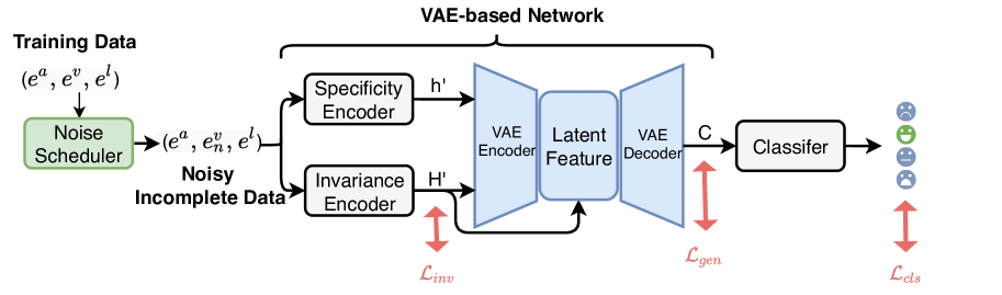
Fig. 1: The main structure of the NMER model, including a noise scheduler, VAE-based network, and the classifier. Three losses are calculated during the training process.

2.3 VAE-based Network

The VAE-based Network includes Specificity and Invariance Encoders [4] and VAE Module. The Specificity Encoder and Invariance Encoder will extract the modality-specific feature $h^{\prime}$ and modality-invariant feature $H^{\prime}$ from the noisy embedding, as similar with [4].

Upon inputting $h^{\prime}$ and $H^{\prime}$ into the VAE Module, they undergo compressing and mapping through the encoder network, yielding mean and variance parameters in the latent space. This transformation effectively shifts the feature from the original data space to a distribution within the latent space. Subsequently, employing a stochastic sampling process and leveraging the reparameterization trick [13] enables the generation of samples based on the latent space distribution. These samples serve as representations of the input feature within the latent space. Moving forward, the latent variable is passed through the decoder network, which reconstructs the embedding by mapping it back to the original data space, thus generating reconstructed multimodal joint representation $C$. Note that the invariant feature $H^{\prime}$ serves as the guidance signal to guide the decoding process.

Throughout the compression, sampling, and reconstruction process above, noisy features will be transformed into normal ones, that is to achieve the denoising effect. The output of the decoder, multimodal joint representation $C$, will be transmitted to the Classifier to reach the last result.

2.4 Loss Functions

As shown in Fig. 1, the total loss $\mathcal{L}$ for NMER includes three parts: $\mathcal{L}=\mathcal{L}_{\text{gen}}+\mathcal{L}_{\text{inv}}+\mathcal{L}_{\text{cls}}$, where the invariant loss $\mathcal{L}_{\text{inv}}$ share the same spirits with [4]. $\mathcal{L}_{\text{inv}}$ also adopts the MSE loss style to reduce the distance between the modality-invariant feature $H^{\prime}$ during training (under incomplete conditions) and the real modality-invariant feature $H$. $\mathcal{L}_{\text{cls}}$ adopts the Cross-Entropy loss function to measure and minimize the disparities between the predicted and actual emotion category labels.

Here, Generation loss $\mathcal{L}_{\text{gen}}$ aims to calculate the distance between generation result $C$ and the ground truth multimodal joint representation $\hat{C}$ under full modalities. Note that the $\mathcal{L}_{\text{gen}}$ consists of two items, that are $\mathcal{L}_{\text{kl}}$ and $\mathcal{L}_{\text{mse}}$. $\mathcal{L}_{\text{kl}}$ aims to make the hidden variables generated by the encoder conform to the standard normal distribution, while $\mathcal{L}_{\text{mse}}$ seeks to make the generated multi-modal joint representation more similar to the target that extracted from full modalities.

$$\small\mathcal{L}_{\text{kl}}=\!-\frac{1}{2}\left(\log\sigma^{2}\!\!-\!\sigma^{2}\!\!-\!\!\mu^{2}\!+\!1\right);\quad\mathcal{L}_{\text{mse}}=\frac{1}{N}\sum_{i=1}^{N}(y_{i}-\hat{y_{i}})^{2}$$ (2)

where $\sigma$ is the variance of the distribution of the latent vector while the $\mu$ is the mean; $N$ is the total number of the real values, $y_{i}$ is the real value, and $\hat{y_{i}}$ is the predicted value.

3 Experiments and Results

We validate our NMER model on the Interactive Emotional Dyadic Motion Capture (IEMOCAP) dataset [15]. Following [3, 4], we use four emotion labels: happy, angry, sad, and neutral.

Systems	Noise Types & Intensities
	100 (Avg)				80 (Avg)				60 (Avg)				40 (Avg)				20 (Avg)
	Gaussian noise		Impulse noise		Gaussian noise		Impulse noise		Gaussian noise		Impulse noise		Gaussian noise		Impulse noise		Gaussian noise		Impulse noise
	WA	UA	WA	UA	WA	UA	WA	UA	WA	UA	WA	UA	WA	UA	WA	UA	WA	UA	WA	UA
MEN[3]	0.5325	0.5235	0.5745	0.5748	0.5458	0.5383	0.5892	0.5842	0.5563	0.5461	0.5916	0.5923	0.5663	0.5623	0.6167	0.6166	0.5949	0.5887	0.6517	0.6525
MMIN[3]	0.6615	0.6693	0.6704	0.6801	0.6630	0.6681	0.6756	0.6873	0.6711	0.6798	0.6796	0.6932	0.6791	0.6850	0.6917	0.7044	0.7031	0.7099	0.7135	0.7250
IF-MMIN[4]	0.6641	0.6739	0.6702	0.6788	0.6702	0.6757	0.6801	0.6868	0.6703	0.6813	0.6859	0.6938	0.6812	0.6893	0.6951	0.7062	0.6977	0.7077	0.7150	0.7262
NMER(ours)	0.6673	0.6746	0.6739	0.6818	0.6706	0.6782	0.6853	0.6909	0.6773	0.6854	0.6920	0.7008	0.6831	0.6894	0.7039	0.7129	0.7060	0.7131	0.7249	0.7359
w/o VAE	0.6642	0.6666	0.6693	0.6785	0.6675	0.6710	0.6841	0.6878	0.6741	0.6778	0.6898	0.6954	0.6776	0.6828	0.7017	0.7087	0.7033	0.7059	0.7237	0.7154

Table 1: The results of the comparative study. “(Avg)” means the average performance across the six incomplete conditions.

3.1 Experimental Setup

We follow [3, 4] to extract the original embeddings $e^{a}$, $e^{v}$ and $e^{l}$.The hidden size of the LSTM structure is set to 128. The TextCNN contains 3 convolution blocks with kernel sizes of 3, 4, 5 and the output size of 128. The output size of the Invariance Encoder is also set to 128. The VAE Module includes a Transformer Encoder of 5 layers as the encoder while Linear layers with dimensions of {64, 128, 384} as the decoder. The classifier contains three linear layers of size {384, 128, 4}. The smoothness coefficient parameters $\beta_{start}$ and $\beta_{end}$ are set to 0.01 and 0.5 respectively. The adding schedule $\beta_{schedule}$ is set to “scaled linear”. For Impulse noise, we set the appear frequency $p$ equals to 0.3. Other parameters are the same as before.

Intensities	Testing Conditions
	{a}		{v}		{l}		{a, v}		{a, l}		{v, l}		Avg
	WA	UA	WA	UA	WA	UA	WA	UA	WA	UA	WA	UA	WA	UA
100	0.5855	0.5995	0.5630	0.5530	0.7001	0.7122	0.6658	0.6730	0.7522	0.7653	0.7375	0.7452	0.6673	0.6746
80	0.5965	0.6114	0.5734	0.5690	0.6996	0.7138	0.6699	0.6761	0.7530	0.7657	0.7402	0.7485	0.6706	0.6782
60	0.6055	0.6147	0.5900	0.5801	0.7043	0.7158	0.6766	0.6782	0.7520	0.7650	0.7442	0.7514	0.6773	0.6854
40	0.6067	0.6164	0.6103	0.6035	0.7112	0.7199	0.6734	0.6809	0.7501	0.7620	0.7470	0.7538	0.6831	0.6894
20	0.6408	0.6507	0.6565	0.6557	0.7312	0.7397	0.6910	0.6987	0.7597	0.7718	0.7567	0.7621	0.7060	0.7131

Table 2: The detailed results of our NMER model on the six incomplete conditions under Gaussian noise.

We utilize the AdamW [19] as the optimizer, and use the Lambda LR [20] to dynamically update the learning rate. The initial learning rate is 0.0002. The batch size is set to 128 and the dropout rate is 0.1. We run our experiments with 10-fold cross-validation, where each fold contains 80 epochs, and report the result on the test set. Each result is run three times and averaged to reduce the effect of random initialization of parameters.

3.2 Comparative Study

We have developed three advanced MER models as our baselines for comparison. 1) Modality Encoder Network (MEN) [3] is a complete-modality baseline that is training on the complete modality condition and inference on the incomplete modality condition [3]; 2) MMIN [3] exploiting cascade residual AutoEncoder and cycle consistency construction to learn joint representations during predicting missing modalities; 3) IF-MMIN [4] improves MMIN by introducing the modality invariant feature to learn the robust joint representations. MMIN and IF-MMIN are treated as the incomplete-modality baselines. We also conduct an ablation study that removes the VAE module, denoted as “w/o VAE”. Specifically, we directly concatenate the $h^{\prime}$ and $H^{\prime}$ and feed them into the classifier.

3.3 Results

We use Weighted Accuracy (WA) [21] and Unweighted Accuracy (UA) [22] to evaluate baselines and our model. Note that we adjust the noise intensity with [20, 40, 60, 80, 100] of two noise types to observe the performance. The average results, across the six incomplete conditions , including {a}, {v}, {l}, {a, v}, {a, l} and {v, l}, of the comparative study are shown in Table 1.

Main Results: 1) From the WA and UA values in rows 2 through 5, we can clearly see that our NMER model outperforms all baselines across various noise intensities and types. For example, for Gaussian noise with 100 intensity, the WA of NMER achieves 0.6673, while MEN, MMIN, and IF-MMIN perform 0.5325, 0.6615, and 0.6641 respectively. UA results also show a similar trend. The above observation illustrates the superior capability of NMER in effectively handling noise-induced challenges. 2) In addition, we also note that the performance of all models experiences various amplitudes decline as the noise intensity increases. More importantly, our model is least affected by different noise intensities. For example, the WA of the MEN model under Gaussian noise decreases from 0.5949 to 0.5325 during the noise intensity increases from 20 to 100. The degradation in baseline systems can be attributed to the loss of information caused by noise and the dimension reduction in the AutoEncoder [23]. This decline proves the effectiveness of our noise scheduler, allowing precise control over noise intensities and simulating various real-world scenarios and noise situations. 3) The obvious discrepancy of WA (approximately 10%) between the complete-modality baseline (row 2 in Table 1) and incomplete-modality baselines (rows 3 to 5 in Table 1) shows the importance of using incomplete training data. It is observed that we can utilize the noise scheduler to simulate different incomplete situations in real-world scenarios and directly predict the robust multimodal joint representation from noisy data, thus answering the two questions mentioned in Section 1 correspondingly.

Ablation Results:

The result of row 6 in Table 1 shows the crucial role of the VAE Module. For example, under Gaussian noise, the WA of the ablation study achieves 0.6776 on the noise intensity 40 whereas the NMER achieves 0.6831, The outcomes clearly indicate that the inclusion of this module contributes to the overall performance of our NMER model. This finding underscores the importance and effectiveness of integrating the VAE component into our framework.

Analysis Results: Furthermore, we report the comprehensive results obtained under six distinct incomplete conditions for NMER in Table 2. We can see that the WA of our model under condition {a} increases from 0.5855 to 0.6408, and the average WA increases from 0.6673 to 0.7060 as the noise intensity decreases from 100 to 20. This observation highlights the model’s remarkable ability to handle varying levels of incompleteness with increasing precision and accuracy. Additionally, it is essential to acknowledge the limitations of previous studies that employed isolated noise settings, as they lacked precise control over noise intensity and failed to facilitate meaningful comparisons across different noise types and intensities. In contrast, our experiments showcase the effectiveness of the noise scheduler in regulating both noise type and intensity, thus enabling comprehensive evaluations and yielding more reliable and insightful results.

3.4 Loss Function Visualization

To further validate the learning capably of $\mathcal{L}_{\text{gen}}$, we visualize the convergence trajectory in Fig. 2. We must confirm the accuracy of our model’s generation to make our model work properly. Therefore, we conduct an analysis of the loss between the multimodal joint representation generated by our model and the original embedding, as illustrated in Fig. 2. The convergence trajectory indicates that the generated multimodal joint representation $C$ is approaching the ground truth multimodal joint representation $\hat{C}$ that is trained with complete-modality data, which validates the effectiveness of $\mathcal{L}_{\text{gen}}$.

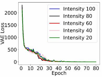
Fig. 2: The convergence trajectory of $\mathcal{L}_{\text{gen}}$, that take Gaussian noise as an example.

4 Conclusion

This work proposed a Noise-robust Multimodal Emotion Recognition model (NMER) that effectively mitigates the impact of incomplete data and generates robust multimodal joint representations, successfully addressing the challenge of incomplete modalities. Experimental results on the IEMOCAP dataset showcase that our NMER achieves state-of-the-art performance across all incomplete conditions, noise types, and intensities. The ablation study also further validates the effectiveness of VAE module. As part of future work, we will improve the model architecture to adapt more types of noise and more complex realistic scenarios.

References

- [1] Rui Liu, Berrak Sisman, Björn W. Schuller, Guanglai Gao, and Haizhou Li, “Accurate emotion strength assessment for seen and unseen speech based on data-driven deep learning,” in Interspeech 2022, 23rd Annual Conference of the International Speech Communication Association, Incheon, Korea, 18-22 September 2022. 2022, pp. 5493–5497, ISCA.
- [2] Kun Zhou, Berrak Sisman, Rui Liu, and Haizhou Li, “Seen and unseen emotional style transfer for voice conversion with a new emotional speech dataset,” in ICASSP 2021-2021 IEEE International Conference on Acoustics, Speech and Signal Processing (ICASSP). IEEE, 2021, pp. 920–924.
- [3] Jinming Zhao, Ruichen Li, and Qin Jin, “Missing modality imagination network for emotion recognition with uncertain missing modalities,” in Proceedings of the 59th Annual Meeting of the Association for Computational Linguistics and the 11th International Joint Conference on Natural Language Processing (Volume 1: Long Papers), 2021, pp. 2608–2618.
- [4] Haolin Zuo, Rui Liu, Jinming Zhao, Guanglai Gao, and Haizhou Li, “Exploiting modality-invariant feature for robust multimodal emotion recognition with missing modalities,” in ICASSP 2023-2023 IEEE International Conference on Acoustics, Speech and Signal Processing (ICASSP). IEEE, 2023, pp. 1–5.
- [5] Zheng Lian, Lan Chen, Licai Sun, Bin Liu, and Jianhua Tao, “Gcnet: graph completion network for incomplete multimodal learning in conversation,” IEEE Transactions on Pattern Analysis and Machine Intelligence, 2023.
- [6] Jiayi Chen and Aidong Zhang, “Hgmf: heterogeneous graph-based fusion for multimodal data with incompleteness,” in Proceedings of the 26th ACM SIGKDD international conference on knowledge discovery & data mining, 2020, pp. 1295–1305.
- [7] Lei Cai, Zhengyang Wang, Hongyang Gao, Dinggang Shen, and Shuiwang Ji, “Deep adversarial learning for multi-modality missing data completion,” in Proceedings of the 24th ACM SIGKDD international conference on knowledge discovery & data mining, 2018, pp. 1158–1166.
- [8] Qiuling Suo, Weida Zhong, Fenglong Ma, Ye Yuan, Jing Gao, and Aidong Zhang, “Metric learning on healthcare data with incomplete modalities.,” in IJCAI, 2019, pp. 3534–3540.
- [9] Changde Du, Changying Du, Hao Wang, Jinpeng Li, Wei-Long Zheng, Bao-Liang Lu, and Huiguang He, “Semi-supervised deep generative modelling of incomplete multi-modality emotional data,” in Proceedings of the 26th ACM international conference on Multimedia, 2018, pp. 108–116.
- [10] Jing Han, Zixing Zhang, Zhao Ren, and Björn Schuller, “Implicit fusion by joint audiovisual training for emotion recognition in mono modality,” in ICASSP 2019-2019 IEEE International Conference on Acoustics, Speech and Signal Processing (ICASSP). IEEE, 2019, pp. 5861–5865.
- [11] Hai Pham, Paul Pu Liang, Thomas Manzini, Louis-Philippe Morency, and Barnabás Póczos, “Found in translation: Learning robust joint representations by cyclic translations between modalities,” in Proceedings of the AAAI Conference on Artificial Intelligence, 2019, vol. 33, pp. 6892–6899.
- [12] Jiandian Zeng, Jiantao Zhou, and Tianyi Liu, “Mitigating inconsistencies in multimodal sentiment analysis under uncertain missing modalities,” in Proceedings of the 2022 Conference on Empirical Methods in Natural Language Processing, 2022, pp. 2924–2934.
- [13] Diederik P Kingma and Max Welling, “Auto-encoding variational bayes,” arXiv preprint arXiv:1312.6114, 2013.
- [14] Kihyuk Sohn, Honglak Lee, and Xinchen Yan, “Learning structured output representation using deep conditional generative models,” Advances in neural information processing systems, vol. 28, 2015.
- [15] Carlos Busso, Murtaza Bulut, Chi-Chun Lee, Abe Kazemzadeh, Emily Mower, Samuel Kim, Jeannette N Chang, Sungbok Lee, and Shrikanth S Narayanan, “Iemocap: Interactive emotional dyadic motion capture database,” Language resources and evaluation, vol. 42, no. 4, pp. 335–359, 2008.
- [16] Carl Friedrich Gauss, Theoria motus corporum coelestium in sectionibus conicis solem ambientium, vol. 7, FA Perthes, 1877.
- [17] Seong Rag Kim and Adam Efron, “Adaptive robust impulse noise filtering,” IEEE Transactions on Signal Processing, vol. 43, no. 8, pp. 1855–1866, 1995.
- [18] Jonathan Ho, Ajay Jain, and Pieter Abbeel, “Denoising diffusion probabilistic models,” Advances in neural information processing systems, vol. 33, pp. 6840–6851, 2020.
- [19] Ilya Loshchilov and Frank Hutter, “Decoupled weight decay regularization,” in International Conference on Learning Representations, 2019.
- [20] Neo Wu, Bradley Green, Xue Ben, and Shawn O’Banion, “Deep transformer models for time series forecasting: The influenza prevalence case,” arXiv preprint arXiv:2001.08317, 2020.
- [21] Ishwar Baidari and Nagaraj Honnikoll, “Accuracy weighted diversity-based online boosting,” Expert Syst. Appl., vol. 160, pp. 113723, 2020.
- [22] Shruti Gupta, Md. Shah Fahad, and Akshay Deepak, “Pitch-synchronous single frequency filtering spectrogram for speech emotion recognition,” Multim. Tools Appl., vol. 79, no. 31-32, pp. 23347–23365, 2020.
- [23] Pascal Vincent, Hugo Larochelle, Isabelle Lajoie, Yoshua Bengio, Pierre-Antoine Manzagol, and Léon Bottou, “Stacked denoising autoencoders: Learning useful representations in a deep network with a local denoising criterion.,” Journal of machine learning research, vol. 11, no. 12, 2010.