kpz-type equation from growth driven by a non-Markovian diffusion

Abstract.

We study a stochastic geometric flow that describes a growing submanifold $\mathds{M}({t})\subseteq\mathbb{R}^{\mathrm{d}+1}$. It is an spde that comes from a continuum version of origin-excited random walk or once-reinforced random walk [3, 7, 26, 27, 28]. It is given by simultaneously smoothing and inflating the boundary of $\mathds{M}({t})$ in a neighborhood of the boundary trace of a reflecting Brownian motion. We show that the large-scale fluctuations of an associated height function are given by a regularized Kardar-Parisi-Zhang (kpz)-type equation on a submanifold in $\mathbb{R}^{\mathrm{d}+1}$, modulated by a Dirichlet-to-Neumann operator. This is shown in any dimension $\mathrm{d}\geqslant 1$. We also prove that in dimension $\mathrm{d}+1=2$, the regularization in this kpz-type spde can be removed after renormalization. Thus, in dimension $\mathrm{d}+1=2$, fluctuations of the geometric flow have a double-scaling limit given by a singular kpz-type equation. To our knowledge, this is the first instance of kpz-type behavior in stochastic Laplacian growth models, which was asked about (for somewhat different models) in [33, 35].

February 27, 2024

1. Introduction

Stochastic interfaces driven by harmonic measure provide rich models for many biological and physical processes, including (internal) diffusion-limited aggregation [30, 40], dielectric breakdown [32], as well as the Hastings-Levitov process [21], the last of which also has connections to turbulence in fluid mechanics. Because the driving mechanism for the growth is determined by harmonic measure, such interfaces are often known as (stochastic) Laplacian growth models.

A central question concerns the large-scale behavior of these interfaces [3, 7, 26, 27, 28]. In [35], the authors asked whether or not the stochastic interface studied therein has a Kardar-Parisi-Zhang (kpz) scaling limit (given by a stochastic pde such as (1.9)). (See also [33] in the physics literature, which addresses a related question for diffusion-limited aggregation, namely its relation to the so-called “Eden model”.) Since then, the question of rigorously deriving kpz asymptotics in stochastic Laplacian growth models more generally has remained open, despite surging interest in kpz universality over the past few decades [4, 5, 34, 41].

The goal of this paper is to derive kpz-type asymptotics for a Laplacian growth model given by a stochastic geometric flow. It is a stochastic pde derived from a continuum version the origin-excited random walk and once-reinforced random walk with strong reinforcement, whose history and background is addressed at length in [3, 7, 26, 27, 28]. In this paper, we show the following two results.

1. Fluctuations of an associated “height function” to this stochastic flow converge (in some scaling limit) to a regularized kpz-type equation. (See Theorem 1.5.)

2. After renormalization, solutions to the aforementioned kpz-type equation converge as we remove the regularization; this is done on hypersurfaces of dimension $\mathrm{d}=1$ in $\mathbb{R}^{2}$. (See Theorem 1.6.)

Throughout this paper, we often use subscripts for inputs at which we evaluate functions of space, time, or space-time. This is in lieu of parentheses, which would make formulas and displays too overloaded.

1.1. kpz universality for the growth model

Let us first give an intuitive description of the model. (Refer to Construction 1.1 for the exact flow pde we will study.)

• Consider the following evolving submanifold $\mathds{M}({t})\subseteq\mathbb{R}^{\mathrm{d}+1}$. First, fix ${t}\geqslant 0$. Take a reflecting Brownian motion $\mathfrak{z}$ in $\mathds{M}({t})$ with inward-normal reflection. Set $\mathfrak{y}^{\varepsilon}_{{t}}$ to be the value of $\mathfrak{z}$ stopped when its boundary local time equals $\varepsilon^{-4/3}{t}$. (Here, $\varepsilon>0$ is a small scaling parameter. See Remark 1.2 and Section 1.3.3 for a discussion of the exponent $-4/3$. Also, by boundary local time, we mean the process that is formally written ${s}\mapsto\int_{0}^{{s}}\delta[\mathfrak{z}_{{r}}\in\partial\mathds{M}[{r}]]\mathrm{d}{r}$ and rigorously constructed by usual regularization of the delta function.) By construction, we know $\mathfrak{y}^{\varepsilon}_{{t}}\in\partial\mathds{M}({t})$ with probability $1$ for all ${t}$. Lastly, since $\mathfrak{y}^{\varepsilon}$ moves at a fast speed of $\varepsilon^{-4/3}$, we expect “homogenization”, i.e. its small-$\varepsilon$ contribution to average out.

• The dynamics of $\mathds{M}({t})$ are given by two mechanisms. The first is “inflating” $\mathds{M}({t})$ smoothly and locally near $\mathfrak{y}^{\varepsilon}_{{t}}$ at constant speed. The second is simultaneously smoothing $\partial\mathds{M}({t})$ using a heat flow. This second ingredient is needed to make sure that the small-$\varepsilon$ scaling limit that we will take for $\mathds{M}({t})$ is well-defined, for example. (The use of a heat flow to regularize the interface is a natural choice, especially in the context of kpz growth [4, 23].) See Sections 1.3.3 and 1.4 for more on this heat-flow smoothing of $\partial\mathds{M}({t})$ (and what happens if we drop it from the growth dynamics).

The model here strongly resembles those of [1, 8, 9]; see Section 1.3.3 for further discussion. The notation $\mathfrak{y}^{\varepsilon}$ and $\mathfrak{z}$ will not be used in the sequel, since we will shortly reparameterize these processes.

A discrete-time, discrete-step version of the above model would be given by running a reflecting Brownian motion inside $\mathds{M}({t})$ until its boundary local time is equal to $\varepsilon^{-4/3}$. At the stopping location of this Brownian motion, augment $\mathds{M}({t})$ by adding a smooth, localized bump. Then, smooth the interface $\partial\mathds{M}({t})$ via heat flow. Finally, we iterate, but with the new starting location of the Brownian particle and the updated, augmented set. The above continuum construction (with inflation) is just more convenient to analyze; we expect the two to have the same large-scale behavior. See Figure 1 for the discrete version.

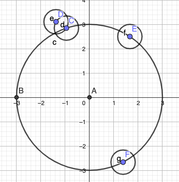
Figure 1. A discrete-time version of the model when the initial set $\mathds{M}$ is a circle centered at point $\mathbf{A}$ (and without the extra heat flow step). Start with $\mathbf{B}$ (on the left). $\mathbf{C}$ is sampled by starting reflecting Brownian motion $\mathbf{B}$ and stopping when its boundary local time hits $\varepsilon^{-4/3}$. At $\mathbf{C}$, add a small ball. $\mathbf{D}$ is sampled by starting reflecting Brownian motion on the augmented set at $\mathbf{C}$, and stopping when the boundary local time hits $\varepsilon^{-4/3}$. Augment the set by adding a circle centered at $\mathbf{D}$. Iterate to sample $\mathbf{E}$, $\mathbf{F}$, and their respective circles.

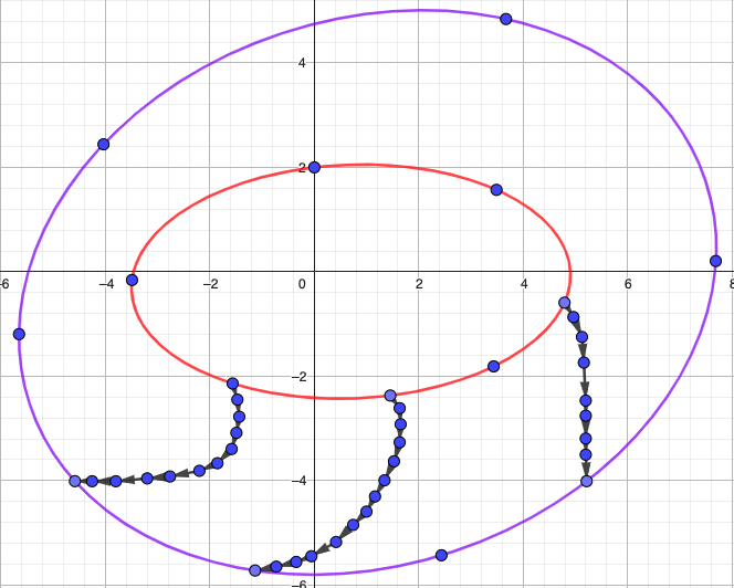
Figure 3. A slightly more sophisticated example (again, of a deterministic approximation to $\mathds{M}({t})$). In this case, $\partial\mathds{M}$ is the red conic section; $\partial\mathds{M}(1)$ is the purple conic section. Three examples of the evolving vector field that one takes to go from $\partial\mathds{M}$ to $\partial\mathds{M}(1)$.

As is often the case, for example with mean curvature flow, it is more convenient for analysis to think of the manifold process $\mathds{M}({t})$ in terms of an evolving (stochastic) function on the boundary $\partial\mathds{M}$ of the initial set $\mathds{M}(0)=\mathds{M}$. Precisely, there is an outward-pointing vector field on $\partial\mathds{M}({t})$ (which determines the “direction” of inflation), which one can pullback to an evolving vector field on $\partial\mathds{M}$. Given this time-dependent vector field on $\partial\mathds{M}$, one can then reconstruct $\mathds{M}({t})$ by taking any point on ${x}\in\partial\mathds{M}$, and following the vector field for some “length” or “height”, which we denote by $\mathbf{I}^{\varepsilon}_{{t},{x}}$. See Figures 2 and 3. This description of $\mathds{M}({t})$ only holds (in principle) until the diffeomorphism class of $\mathds{M}({t})$ changes. If the diffeomorphism class changes at time $\mathfrak{t}$, there can exist a point on $\partial\mathds{M}(\mathfrak{t})$ which can be arrived at by following vector fields starting at two different points on $\partial\mathds{M}$; this makes the construction ill-defined. In this paper, we assume the diffeomorphism class does not change. See Section 1.5 for a further discussion.

Thus, the $\varepsilon\to 0$ asymptotics of $\mathds{M}({t})$ amount to those of the vector field process and the $\mathbf{I}^{\varepsilon}$ process. In this paper, we focus on the latter, which we formulate as follows. (In particular, we make precise “inflation”.) We explain Construction 1.1 in detail afterwards. Again, refer to Remark 1.2 and Section 1.3.3 for more on the choice of exponents $-1/3$ and $-4/3$ appearing below.

Construction 1.1.

Fix $\mathrm{d}\geqslant 1$, and take a compact, connected subset $\mathds{M}\subseteq\mathbb{R}^{\mathrm{d}+1}$ with smooth boundary $\partial\mathds{M}$. Let ${t}\mapsto(\mathbf{I}^{\varepsilon}_{{t},\cdot},\mathfrak{q}^{\varepsilon}_{{t}})\in\mathscr{C}^{\infty}(\partial\mathds{M})\times\partial\mathds{M}$ be the following Markov process.

1. With notation to be explained afterwards, we let $\mathbf{I}^{\varepsilon}$ solve

   $$\partial_{{t}}\mathbf{I}^{\varepsilon}_{{t},{x}}=\Delta_{\partial\mathds{M}}\mathbf{I}^{\varepsilon}_{{t},{x}}+\varepsilon^{-\frac{1}{3}}\mathrm{Vol}_{\mathbf{I}^{\varepsilon}_{{t}}}\mathbf{K}_{{x},\mathfrak{q}^{\varepsilon}_{{t}}}.$$ (1.1)

   • $\Delta_{\partial\mathds{M}}$ is the Laplacian on the embedded manifold $\partial\mathds{M}$.

   • For any $\mathbf{I}\in\mathscr{C}^{\infty}(\partial\mathds{M})$, the term $\mathrm{Vol}_{\mathbf{I}}$ is the volume of the image of $\partial\mathds{M}$ under $\mathbf{I}$, i.e. the volume of its graph. By a standard change-of-variables computation, we have

     $$\mathrm{Vol}_{\mathbf{I}}={{}\int_{\partial\mathds{M}}}(1+|\nabla_{\partial\mathds{M}}\mathbf{I}_{{z}}|^{2})^{\frac{1}{2}}\mathrm{d}{z},$$ (1.2)

     where $\mathrm{d}{z}$ is integration with respect to surface measure on $\partial\mathds{M}$.

   • The kernel $\mathbf{K}\in\mathscr{C}^{\infty}(\partial\mathds{M}\times\partial\mathds{M})$ is real-valued, symmetric, and it satisfies $\int_{\partial\mathds{M}}\mathbf{K}_{{x},{z}}\mathrm{d}{z}=1$.

2. We now define $\mathfrak{q}^{\varepsilon}$ to be $\mathfrak{b}$ stopped when its boundary local time is equal to $\varepsilon^{-4/3}{t}$, where $\mathfrak{b}$ is a reflecting Brownian motion on $\mathds{M}$ with metric determined by $\mathbf{I}^{\varepsilon}$. Precisely:

   • For any $\mathbf{I}\in\mathscr{C}^{\infty}(\partial\mathds{M})$, consider the graph map $\partial\mathds{M}\to\partial\mathds{M}\times\mathbb{R}$ given by ${x}\mapsto({x},\mathbf{I}_{{x}})$. Equip $\partial\mathds{M}\times\mathbb{R}$ with the product metric (here $\partial\mathds{M}$ is given Euclidean surface metric). Let $\mathbf{g}[\nabla_{\partial\mathds{M}}\mathbf{I}]$ be the pullback of this metric under $\mathbf{I}$. (It is a metric on $\partial\mathds{M}$. This notation is used since it depends only on first-order derivatives of $\mathbf{I}$.) Extend $\mathbf{g}[\nabla_{\partial\mathds{M}}\mathbf{I}]$ from $\partial\mathds{M}$ to $\mathds{M}$ smoothly.

   • Let $\mathfrak{b}$ be reflecting Brownian motion on $\partial\mathds{M}$ with respect to the time-dependent metric $\mathbf{g}[\nabla_{\partial\mathds{M}}\mathbf{I}^{\varepsilon}_{{t}}]$. (So, its infinitesimal generator at time ${t}$ is Laplacian on $\mathds{M}$ with metric $\mathbf{g}[\nabla_{\partial\mathds{M}}\mathbf{I}^{\varepsilon}_{{t}}]$.)

The submanifold $\mathds{M}$ is the initial data for $\mathds{M}(t)$.

As we mentioned earlier, the Laplacian in (1.1) is a canonical smoothing operator to consider for interface growth. This term describes the heat-flow smoothing of the interface. Again, see Section 1.4 for what happens without it. The second term on the RHS of (1.1) is the smooth “inflation” (the kernel $\mathbf{K}$ determines the “shape” of the inflating set). Also, $\mathrm{Vol}$ on the RHS of (1.1) is a global factor to normalize the speed of growth at any point. (Without it, $\varepsilon\to 0$-limits in this paper would be non-local; we explain this shortly.)

Let us also explain extending $\mathbf{g}[\nabla_{\partial\mathds{M}}\mathbf{I}]$ from $\partial\mathds{M}$ to $\mathds{M}$. Allowing for any smooth extension is essentially the same as allowing the outwards flow of $\partial\mathds{M}$ to be in the direction of any smooth outward vector field on $\partial\mathds{M}$. This is some hint of universality (see also Section 1.4).

Construction 1.1 is not just an isolated construction. It is an spde that one derives from the description given before Figure 1 (given an appropriate, precise formulation of that model).

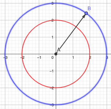
Figure 2. Example (of a deterministic approximation to $\mathds{M}({t})$) when $\mathds{M}$ is the disk with boundary equal to the red circle. The disk with blue boundary is $\mathds{M}({t})$ at ${t}=1$. In this case, every point in $\partial\mathds{M}(1)$ can be obtained by following the outwards radial vector field for length $1$, starting at a point on the red circle $\partial\mathds{M}$. (For a picture for $\mathds{M}(1)$ instead of its deterministic approximation, just add fluctuations in the radial direction at each point in the blue circle.)

It turns out that $\mathbf{I}^{\varepsilon}$ has an uninteresting limit as $\varepsilon\to 0$; in this limit, we ultimately have $\mathbf{I}^{\varepsilon}_{{t},{x}}-\varepsilon^{-1/3}{t}\to 0$ locally uniformly in $({t},{x})$. Indeed, if one believes that the $\mathfrak{q}^{\varepsilon}$ averages out because it moves at the very fast speed of $\varepsilon^{-4/3}$, then the growth model essentially inflates at speed $1$ at every point on the boundary. (Without the $\mathrm{Vol}$ factor on the RHS of (1.1), the model instead samples a point uniformly at random on the interface to inflate from.) What is more interesting is the following fluctuation field:

$$\mathbf{Y}^{\varepsilon}_{{t},{x}}=\varepsilon^{-\frac{1}{3}}[\mathbf{I}^{\varepsilon}_{{t},{x}}-\varepsilon^{-\frac{1}{3}}{t}].$$ (1.3)

Remark 1.2.

Let us explain the choice of scaling in Construction 1.1 and (1.3). The equation (1.1) describes a fast-moving particle of speed $\varepsilon^{-4/3}$ that induces speed $\varepsilon^{-1/3}$ growth of the interface. This is the same as speeding time (by $\varepsilon^{-4/3}$) a process with a speed $1$ particle and speed $\varepsilon$ growth. The deterministic, leading-order “shape theorem” behavior of the interface occurs at time-scales of speed $\varepsilon^{-1}$, in which the particle has speed $\varepsilon^{-1}$ and the interface growth has speed $1$. On top of this, if we additionally scale time by $\varepsilon^{-1/3}$, which gives (1.1) and (1.3), we obtain nontrivial fluctuations. This is what (1.1) and (1.3) imply as far as scaling is concerned. We could have defined $\mathbf{I}^{\varepsilon}$ to have speed $\varepsilon^{-1}$ and then speed it up by $\varepsilon^{-1/3}$, which is perhaps more natural. But, this would have been notationally more involved.

The scaling used (to go from the asymptotic shape to fluctuations) of time and of the fluctuation itself are the same factor (here, it is $\varepsilon^{-1/3}$). This is the case for (many) kpz models more generally [4, 29, 34].

Assumption 1.3.

Assume that $\mathbf{Y}^{\varepsilon}_{0,\cdot}=\mathbf{Y}^{\mathrm{init}}_{0,\cdot}$ for some $\mathbf{Y}^{\mathrm{init}}_{0,\cdot}\in\mathscr{C}^{\infty}(\partial\mathds{M},\mathbb{R})$ independent of $\varepsilon$.

It turns out that the small-$\varepsilon$ limit of $\mathbf{Y}^{\varepsilon}$ is given by the following spde, which we explain afterwards:

$$\partial_{{t}}\mathfrak{h}^{\mathbf{K}}_{{t},{x}} =\Delta_{\partial\mathds{M}}\mathfrak{h}^{\mathbf{K}}_{{t},{x}}+{{}\int_{\partial\mathds{M}}}\mathbf{K}_{{x},{z}}|\nabla_{\partial\mathds{M}}\mathfrak{h}^{\mathbf{K}}_{{t},{z}}|^{2}\mathrm{d}{z}+{{}\int_{\partial\mathds{M}}}[\mathbf{K}_{{x},{z}}-1](-\mathscr{L})^{-\frac{1}{2}}\xi_{{t},{z}}\mathrm{d}{z}$$ (1.4)

$$\mathfrak{h}^{\mathbf{K}}_{0,\cdot} =\mathbf{Y}^{\mathrm{init}}_{0,\cdot}.$$

Technically, by (1.4), we mean the Duhamel representation below (see Lemma A.2):

$$\mathfrak{h}^{\mathbf{K}}_{{t},{x}} =\{\exp[{t}\Delta_{\partial\mathds{M}}]\mathbf{Y}^{\mathrm{init}}_{0,\cdot}\}_{{x}}+{{}\int_{0}^{{t}}}\left\{\exp[({t}-{s})\Delta_{\partial\mathds{M}}]{{}\int_{\partial\mathds{M}}}\mathbf{K}_{\cdot,{z}}|\nabla_{\partial\mathds{M}}\mathfrak{h}^{\mathbf{K}}_{{s},{z}}|^{2}\mathrm{d}{z}\right\}_{{x}}\mathrm{d}{s}$$ (1.5)

$$+{{}\int_{0}^{{t}}}\left\{\exp[({t}-{s})\Delta_{\partial\mathds{M}}]{{}\int_{\partial\mathds{M}}}[\mathbf{K}_{\cdot,{z}}-1](-\mathscr{L})^{-\frac{1}{2}}\xi_{{t},{z}}\mathrm{d}{z}\right\}_{{x}}\mathrm{d}{s}.$$ (1.6)

Let us now explain the notation used in this spde.

• $\exp[\mathfrak{t}\Delta_{\partial\mathds{M}}]$ is the associated heat semigroup for $\Delta_{\partial\mathds{M}}$, and $\nabla_{\partial\mathds{M}}$ denotes gradient on $\partial\mathds{M}$.

• $\mathscr{L}$ denotes the Dirichlet-to-Neumann map on $\mathds{M}$. Given any $\varphi\in\mathscr{C}^{\infty}(\partial\mathds{M})$, the function $\mathscr{L}\varphi$ is defined to be ${x}\mapsto\nabla_{\mathsf{N}[{x}]}\mathscr{U}^{\varphi}_{{x}}$, where $\nabla_{\mathsf{N}[{x}]}$ is gradient in the unit inwards normal direction at ${x}\in\partial\mathds{M}$, and $\mathscr{U}^{\varphi}$ is the harmonic extension of $\varphi$ to $\mathds{M}$ (so that $\Delta\mathscr{U}^{\varphi}=0$, where $\Delta$ is Laplacian on $\mathds{M}\subseteq\mathbb{R}^{\mathrm{d}+1}$).

  It turns out that $\mathscr{L}$ is a self-adjoint operator with core $\mathscr{C}^{\infty}(\partial\mathds{M})$ (with respect to the surface measure on $\partial\mathds{M}$, i.e. the Riemannian measure induced by surface metric on $\partial\mathds{M}$). It is negative semi-definite, and it has a discrete spectrum. Also, its null-space is one-dimensional; it is spanned by constant functions on $\partial\mathds{M}$. So, $(-\mathscr{L})^{-1/2}$ on the RHS of (1.9) is well-defined, since the function ${z}\mapsto\mathbf{K}_{{x},{z}}-1$ is orthogonal to the null-space of $\mathscr{L}$ (i.e. it has vanishing integral on $\partial\mathds{M}$ for any ${x}$). See Lemma B.1.

• $\xi$ is a space-time white noise on $[0,\infty)\times\partial\mathds{M}$. Intuitively, it is the Gaussian field with covariance kernel $\mathbb{E}\xi_{{t},{x}}\xi_{{s},{y}}=\delta_{{t}={s}}\delta_{{x}={y}}$. More precisely, for any orthonormal basis $\{e_{{k}}\}_{{k}}$ of $\mathrm{L}^{2}(\partial\mathds{M})$ (e.g. the eigenbasis for $\mathscr{L}$), it has the following representation (in the language of Ito calculus), where $b_{{t},k}$ are independent standard Brownian motions:

  $$\xi_{{t},\cdot}\mathrm{d}t=\sum_{{k}}\mathrm{d}b_{{t},k}e_{k}.$$ (1.7)

We emphasize that (1.4) is essentially the usual kpz equation (see [4, 23]) except for two differences. The first is the regularization kernel $\mathbf{K}$; we will shortly consider the delta-function limit for $\mathbf{K}$ in the case $\mathrm{d}=1$. The second is the $(-\mathscr{L})^{-1/2}$ operator. We explain this term immediately after Theorem 1.5.

Before we state the first main result (convergence of $\mathbf{Y}^{\varepsilon}\to\mathfrak{h}^{\mathbf{K}}$), we comment on well-posedness of (1.4). By smoothing of the $\Delta_{\partial\mathds{M}}$ semigroup (see Lemma A.3) and because $\mathscr{L}$ maps smooth functions to smooth functions (see Lemma B.1), it is not hard to see that (1.5)-(1.6) is locally well-posed in $\mathscr{C}^{2}(\partial\mathds{M})$ (until a possibly random and finite stopping time denoted by $\tau_{\mathfrak{h}^{\mathbf{K}}}$).

Finally, let us introduce the following notion of high probability (to be used throughout this paper).

Definition 1.4.

We say an event $\mathscr{E}$ holds with high probability if $\mathbb{P}[\mathscr{E}]\to 1$ as $\varepsilon\to 0$.

Theorem 1.5.

There exists a coupling between $\{\mathbf{Y}^{\varepsilon}\}_{\varepsilon\to 0}$ and $\mathfrak{h}^{\mathbf{K}}$ such that with high probability, for any $\delta>0$ and $0\leqslant\tau\leqslant\tau_{\mathfrak{h}^{\mathbf{K}}}-\delta$, the following holds for some $\kappa[\delta,\varepsilon]\geqslant 0$ that vanishes as $\varepsilon\to 0$:

$$\sup_{0\leqslant{t}\leqslant\tau\wedge 1}\|\mathbf{Y}^{\varepsilon}_{{t},\cdot}-\mathfrak{h}^{\mathbf{K}}_{{t},\cdot}\|_{\mathscr{C}^{2}(\partial\mathds{M})}\leqslant\kappa[\delta,\varepsilon].$$ (1.8)

(Here, $\mathscr{C}^{2}(\partial\mathds{M})$ is the usual space of twice continuously differentiable functions on the manifold $\partial\mathds{M}$. Also, we have used the notation $a\wedge b=\min(a,b)$.)

Theorem 1.5 essentially asserts convergence in law of $\mathbf{Y}^{\varepsilon}$ to $\mathfrak{h}^{\mathbf{K}}$. Because of the need for a stopping time $\tau_{\mathfrak{h}^{\mathbf{K}}}$, we found it most convenient to state it in terms of couplings. Also, the utility of stopping before $1$ is to make sure we work only on compact time-intervals. Of course, there is nothing special about $1$. Finally, we could have used $\mathscr{C}^{{k}}(\partial\mathds{M})$ for any ${k}\geqslant 2$. Going to ${k}=1$, for example, perhaps requires more work.

Theorem 1.5 implies kpz behavior for fluctuations $\mathbf{Y}^{\varepsilon}$ of the stochastic flow at hand. Although (1.4) has the extra $(-\mathscr{L})^{-1/2}$-operator that does not show up in the “standard” kpz equation, the implication of Theorem 1.5 is that the stochastic, slope-dependent growth (i.e. the last term in (1.1)) is asymptotically a quadratic function of the slope plus a noise; this indicates kpz behavior. The reason why $(-\mathscr{L})^{-1/2}$ appears in the scaling limit for $\mathbf{Y}^{\varepsilon}$ is because fluctuations in the growth model come from a single Brownian particle which explores the entire manifold. Thus, a non-local operator must hit the noise. (The reason for $\mathscr{L}$ in particular is because $\mathscr{L}$ is the generator for a reflecting Brownian motion on the time-independent manifold $\mathds{M}$ time-changed via boundary local time; see [22].)

Theorem 1.5 holds locally in time (until an $\varepsilon$-independent stopping time). This is more-or-less because we work in the $\mathscr{C}^{2}(\partial\mathds{M})$ topology, not a weaker topology like $\mathscr{C}^{0}(\partial\mathds{M})$, for example; see Remark 1.8.

For a more detailed explanation of why Theorem 1.5 is true, see after Theorems 3.2 and 3.3.

1.2. The singular limit of (1.4)

In (1.4), if we formally replace $\mathbf{K}$ by the delta function on the diagonal of $\partial\mathds{M}\times\partial\mathds{M}$, we get the following spde, which we (formally) pose in any dimension $\mathrm{d}\geqslant 1$:

$$\partial_{{t}}\mathfrak{h}_{{t},{x}}=\Delta_{\partial\mathds{M}}\mathfrak{h}_{{t},{x}}+|\nabla_{\partial\mathds{M}}\mathfrak{h}_{{t},{x}}|^{2}+\Pi^{\perp}(-\mathscr{L})^{-\frac{1}{2}}\xi_{{t},{x}},\quad({t},{x})\in(0,\infty)\times\partial\mathds{M}.$$ (1.9)

Above, $\Pi^{\perp}$ denotes projection away from the null-space of $\mathscr{L}$, i.e. away from the span of constant functions on $\partial\mathds{M}$. Our goal now is to make sense of (1.9) itself, so that we can rigorously show convergence of (1.4) to (1.9) in the limit where $\mathbf{K}$ converges to the delta function. However, (1.9) is not classically well-posed. Indeed, $\mathscr{L}$ is a first-order elliptic pseudo-differential operator, so $(-\mathscr{L})^{-1/2}$ gains half a derivative. But integrating the heat kernel for $\Delta_{\partial\mathds{M}}$ against $\xi$, in dimension $1$, lets us take strictly less than half a derivative. So, we cannot take a full derivative and expect to get a function that we can square to define the quadratic nonlinearity in (1.9). Thus, we must carry out the standard procedure for singular spdes via regularization, renormalization, and showing existence of limits as we remove the regularization (see [6, 17], for example). In particular, we consider the following spde, which we explain afterwards:

$$\partial_{{t}}\mathfrak{h}^{\eta}_{{t},{x}}=\Delta_{\partial\mathds{M}}\mathfrak{h}^{\eta}_{{t},{x}}+|\nabla_{\partial\mathds{M}}\mathfrak{h}^{\eta}_{{t},{x}}|^{2}-\mathscr{C}_{\eta}+\Pi^{\eta}(-\mathscr{L})^{-\frac{1}{2}}\xi_{{t},{x}}.$$ (1.10)

• $\Pi^{\eta}$ is projection onto the direct sum of the first $\lfloor\eta^{-1}\rfloor$-many eigenspaces of $\mathscr{L}$ with non-zero eigenvalues. (By Lemma B.1, the spectrum of $\mathscr{L}$ is discrete. Also, we order eigenspaces by ordering the absolute values of their eigenvalues in increasing order. Thus, $\Pi^{\eta}\to\Pi^{\perp}$ as $\eta\to 0$ in a weak sense.)

• To specify the constant $\mathscr{C}_{\eta}$, we first let $\{\lambda_{\ell}\}_{\ell=1}^{\infty}$ be the non-zero eigenvalues of $-\mathscr{L}$, ordered in the same fashion as the previous bullet point. (Note that $\lambda_{\ell}>0$ for all $\ell\geqslant 1$). Define

  $$\mathscr{C}_{\eta} :=\frac{\pi}{2}{\sum_{\ell=1}^{1/\eta}}\frac{\lambda_{\ell+1}-\lambda_{\ell}}{\lambda_{\ell+1}}.$$ (1.11)

  It can be checked by Lemma B.3 that $\mathscr{C}_{\eta}$ diverges as $\eta\to 0$ for any dimension $\mathrm{d}$; so, (1.9) is “singular”.

Standard pde theory implies that (1.10) is locally well-posed with smooth solutions for any $\eta>0$ fixed. The following result, which restricts to dimension $\mathrm{d}+1=2$, says the $\eta\to 0$ limit of these solutions exists. (Although Theorem 1.6 looks like a standard spde result, we explain shortly why it has geometric content. In particular, we are solving a singular spde on a manifold, whose geometry plays an important role.)

Theorem 1.6.

Suppose $\mathds{M}\subseteq\mathbb{R}^{2}$ is a compact manifold with smooth boundary $\partial\mathds{M}$.

For any $\mathfrak{h}^{\mathrm{initial}}\in\mathscr{C}^{2}(\partial\mathds{M})$ independent of $\eta>0$, the sequence of solutions $\{\mathfrak{h}^{\eta}\}_{\eta>0}$ to (1.10) with initial data $\mathfrak{h}^{\mathrm{initial}}$ converges in probability in the following (analytically) weak sense. There exists a stopping time $\tau_{\eqref{eq:singSPDE}}[\mathfrak{h}^{\mathrm{initial}}]$ such that for any test function $\mathtt{F}\in\mathscr{C}^{\infty}(\mathbb{R}\times\partial\mathds{M})$ and any $\tau\in[0,\tau_{\eqref{eq:singSPDE}}[\mathfrak{h}^{\mathrm{initial}}])$, the sequence of random variables below converges in probability as $\eta\to 0$:

$${{}\int_{[0,\tau)}\int_{\partial\mathds{M}}}\mathtt{F}_{{t},{x}}\mathfrak{h}^{\eta}_{{t},{x}}\mathrm{d}{x}\mathrm{d}{t}.$$ (1.12)

Remark 1.7.

The regularization of (1.9) that we want to study in view of (1.4) is not quite (1.10); the quadratic nonlinearity should be regularized. In particular, if $\Pi^{\eta,\sim}=\Pi^{\eta}+\Pi^{\mathrm{const}}$, where $\Pi^{\mathrm{const}}$ is projection onto the space of constant functions, then we want to replace

$$|\nabla_{\partial\mathds{M}}\mathfrak{h}^{\eta}_{{t},{x}}|^{2}\mapsto\Pi^{\eta,\sim}[|\nabla_{\partial\mathds{M}}\mathfrak{h}^{\eta}_{{t},{x}}|^{2}].$$ (1.13)

The proof of Theorem 1.6 can be used verbatim to handle this change, but several details become noticeably more complicated for entirely technical reasons (e.g. having to estimate the commutator of semigroups of $\Delta_{\partial\mathds{M}}$ and $\mathscr{L}$ using $[\Delta_{\partial\mathds{M}},\mathscr{L}]$; see Lemma B.2). It is for this reason only that we study (1.10).

Remark 1.8.

One can also solve (1.9) by defining the Cole-Hopf map $\mathfrak{h}:=\log\mathfrak{Z}$, where $\mathfrak{Z}$ solves a linear spde. This is likely to give the same object as the limit in Theorem 1.6 for $\mathds{M}\subseteq\mathbb{R}^{2}$. In particular, this gives a possible way to show infinite lifetime for (1.9) (in a topology that is much weaker than $\mathscr{C}^{2}(\partial\mathds{M})$). There is also a chance of using this solution theory to push to $\mathrm{d}>1$. However, this linearization method does not work for the spde alluded to in Remark 1.7, so we do not pursue this here.

Theorem 1.6 states a weak version of convergence for $\mathfrak{h}^{\eta}$. But, it can be upgraded rather easily to a more quantitative convergence using our methods. We do not pursue this here, since it is more of a detail than the main point. (In a similar spirit, the assumption that $\mathfrak{h}^{\mathrm{initial}}$ is in $\mathscr{C}^{2}(\partial\mathds{M})$ is likely sub-optimal, but this is besides the point as well.)

An interesting observation about Theorem 1.6 is that $\mathscr{C}_{\eta}$ in (1.10) is constant in space, even though $\Delta_{\partial\mathds{M}}$ and $\mathscr{L}$ therein look different at different points on $\partial\mathds{M}$ (the metric is varying on $\partial\mathds{M}$). Roughly speaking, the reason why we have constant renormalization in (1.10) comes from the universality (in space) of the so-called local or pointwise Weyl law. This yields pointwise eigenfunction asymptotics (in this case for $\mathscr{L}$) that depend only on eigenvalues of $\mathscr{L}$, not on space or the manifold otherwise. We explain this point more in Section 3.4 along with other geometric-analytic inputs needed to solve (1.9) that seem to be absent in previous studies of singular spdes.

By Theorems 1.5 and 1.6, in the case $\mathrm{d}=1$ (so hypersurfaces in $\mathbb{R}^{2}$), we get a singular kpz-type equation limit for (1.3). In particular, we can take $\mathbf{K}$ in Theorem 1.5 to converge to a delta function on the diagonal of $\partial\mathds{M}\times\partial\mathds{M}$ sufficiently slowly and deduce convergence of $\mathbf{Y}^{\varepsilon}$ to (1.10).

Let us also mention that the analytic topologies used in Theorems 1.5 and 1.6 are quite different ($\mathscr{C}^{2}(\partial\mathds{M})$ versus weak-$\ast$ convergence). As we mentioned above, improving the topology of convergence in Theorem 1.6 is probable, but it is not likely that it holds in $\mathscr{C}^{2}(\partial\mathds{M})$, since (1.10) is a singular spde. Convergence in Theorem 1.5 in a topology weaker than $\mathscr{C}^{2}(\partial\mathds{M})$ seems to be difficult (as noted after Theorem 1.5), since the proof is largely based on elliptic regularity. It would be interesting to close this gap; this would strengthen the double-scaling limit result (e.g. quantify convergence of $\mathbf{K}$ to a delta).

1.3. Background and previous work

1.3.1. KPZ from stochastic geometric flows

To our knowledge, any sort of kpz universality for diffusions interacting with their range has not appeared in the literature (rigorously) before, even though this question had been asked by [35] almost 20 years ago. The closest work, which is still quite different, we are aware of to ours is [19]. However, [19] has randomness coming from a background environment (with mixing and independence-type properties), while the randomness in our flow model comes from a single particle.

1.3.2. Singular spdes on manifolds

While we were completing this work, [20] appeared on the arXiv. It treats spdes on manifolds using regularity structures [17]. The spdes in [20] do not have non-local noise driven by a Dirichlet-to-Neumann operator. This allows [20] to work in Hölder (or Besov) spaces, while we require estimates in $\mathrm{L}^{2}$-based Sobolev spaces to handle $\mathscr{L}$ (see Section 3.4.2). In particular, the spde that we consider in this paper is genuinely different from those in [20]. However, some conclusions derived here and in [20] are similar. For example, renormalization counter-terms in [20] are constant as well. (This is true unless the equation is sufficiently singular, in which case one must also renormalize via scalar curvature. We do not treat this case here.) In [20], this is shown by classical asymptotics of the heat kernel on the manifold. (Given connections between Weyl laws and heat kernels, we expect that our methods are intimately connected.)

1.3.3. Shape theorems

This paper studies fluctuation scaling for the height function, i.e. study (1.3). In [9], we studied (a Poissonization of) the discrete version of Figure 1 without heat flow regularization. The main result of [9] was a shape theorem for the growth model therein, in particular a scaling limit for the evolving vector field process that we alluded to before Construction 1.1, but on time-scale that is slower by a factor of $\varepsilon^{1/3}$ than the one we consider in this paper. In particular, under the scaling of [9], the heat flow term in (1.1) vanishes, so the results of [9] would hold even if we included said term. A similar shape theorem (for more general processes than Brownian motion but for a more restricted spherical geometry) was shown in [8].

1.4. A word about kpz universality

The methods we use require very little about the Brownian nature of the randomness in (1.1). (Indeed, as indicated in Section 3.4.1, only spectral gap estimates are needed.) This can be interpreted as another instance of universality. (Of course, if we change Brownian motion to another process, the $\mathscr{L}$-operator in (1.9) may change. The universal kpz quadratic, however, will not.)

If we drop Laplacians in (1.1) and (3.1), Theorem 1.5 would still hold for the resulting spdes. (Indeed, (3.1) is still a smoothing equation because $\mathbf{K}$ therein is smooth.) In this case, Theorem 1.5 gives a universality result that more resembles the so-called “kpz fixed point” [29]. However, we would not be able to rigorously take the singular limit as in Theorem 1.6.

1.5. Changing diffeomorphism class

We assumed that the diffeomorphism class of the growing set does not change. In general, we can stop the growth process when the diffeomorphism class of the set changes; Theorem 1.5 would remain true. As for global-in-time scaling limits (e.g. what the limit spde should even be) in the case where the diffeomorphism class changes, studying more carefully the Brownian particle may provide key information, similar to [10]. (In [10], singularities in a Stefan pde are resolved using a particle system.)

1.6. Organization of the paper

Section 3 outlines the methods (and essentially proves Theorems 1.6 and 1.5 modulo technicalities to be checked). The rest of the paper is outlined at the end of Section 3.

1.7. Acknowledgements

We thank Martin Hairer and Harprit Singh for useful conversation regarding their recent work. Research supported in part by nsf grant dms-1954337 (A.D.), and by the nsf Mathematical Sciences Postdoctoral Fellowship program under Grant. No. dms-2203075 (K.Y.).

2. Function spaces and other notation

We now give a list of function spaces (and a few other pieces of notation) to be used throughout the paper.

1. For any set $I$ and $a,b\in\mathbb{R}$, when we write $a\lesssim_{I}b$, we mean $|a|\leqslant\Lambda|b|$ for an implied constant $\Lambda\geqslant 0$ depending only on $I$. (If $I$ is a finite subset of $\mathbb{R}^{n}$ for some $n\geqslant 1$, the dependence of $\Lambda$ is assumed to be smooth in the elements of $I$.) By $a\gtrsim_{I}b$, we mean $b\lesssim_{I}a$. By $a\asymp b$, we mean $a\lesssim b$ and $b\lesssim a$ with possibly different implied constants. Also, by $a=\mathrm{O}_{I}(b)$, we mean $a\lesssim_{\mathrm{I}}b$.

2. For any $a,b\in\mathbb{R}$, we define $a\wedge b=\min(a,b)$.

3. When we say $\beta\in\mathbb{R}$ is uniformly positive, we mean $\beta\geqslant C$ for $C>0$ that depends on no parameters.

4. For ${p}\geqslant 1$, let $\mathrm{L}^{{p}}(\partial\mathds{M})$ be the usual $\mathrm{L}^{{p}}$-space, where $\partial\mathds{M}\subseteq\mathbb{R}^{\mathrm{d}+1}$ has Riemannian surface measure.

5. Fix any integer ${k}\geqslant 0$. Fix an orthonormal frame $\mathsf{e}_{1},\ldots,\mathsf{e}_{\mathrm{d}}$ (i.e. a smoothly varying orthonormal basis for tangent spaces of the manifold $\partial\mathds{M}$ with Euclidean surface metric). For smooth $\varphi:\partial\mathds{M}\to\mathbb{R}$, set

   $$\|\varphi\|_{\mathscr{C}^{{k}}(\partial\mathds{M})}:=\sup_{{x}\in\partial\mathds{M}}|\varphi_{{x}}|+\sup_{{x}\in\partial\mathds{M}}\sup_{{i}_{1},\ldots,{i}_{{k}}}|\nabla_{{i}_{1}}\ldots\nabla_{{i}_{{k}}}\varphi_{{t},{x}}|,$$ (2.1)

   where $\nabla_{{i}}$ is gradient in the direction of the orthonormal frame vector $\mathsf{e}_{{i}}$, and the inner supremum is over subsets of size ${k}$ in $\{1,\ldots,\mathrm{d}\}$. Let $\mathscr{C}^{{k}}(\partial\mathds{M})$ be the corresponding closure of smooth functions on $\partial\mathds{M}$.

6. Let $\mathscr{C}^{0,\upsilon}(\partial\mathds{M})$, for $\upsilon\in(0,1)$, be the Hölder norm on the manifold $\partial\mathds{M}$ with Euclidean surface metric).

7. Fix $\mathfrak{t}\geqslant 0$. Let $\mathscr{C}^{\infty}_{\mathfrak{t}}\mathscr{C}^{\infty}_{\partial\mathds{M}}$ be the space of smooth $\varphi:[0,\mathfrak{t}]\times\partial\mathds{M}\to\mathbb{R}$. Fix integers ${k}_{1},{k}_{2}\geqslant 0$, and set

   $$\|\varphi\|_{\mathscr{C}^{{k}_{1}}_{\mathfrak{t}}\mathscr{C}^{{k}_{2}}_{\partial\mathds{M}}}:=\sup_{0\leqslant{t}\leqslant\mathfrak{t}}\left\{\|\partial_{{t}}^{{k}_{1}}\varphi_{{t},\cdot}\|_{\mathscr{C}^{0}(\partial\mathds{M})}+\|\varphi_{{t},\cdot}\|_{\mathscr{C}^{{k}_{2}}(\partial\mathds{M})}\right\},\quad\varphi\in\mathscr{C}^{\infty}_{\mathfrak{t}}\mathscr{C}^{\infty}_{\partial\mathds{M}}.$$ (2.2)

   We let $\mathscr{C}^{{k}_{1}}_{\mathfrak{t}}\mathscr{C}^{{k}_{2}}_{\partial\mathds{M}}$ be the closure of smooth functions on $[0,\mathfrak{t}]\times\partial\mathds{M}$ under this norm.

8. Fix any integer ${k}\geqslant 0$. For any $\varphi:\partial\mathds{M}\to\mathbb{R}$ smooth, we define

   $$\|\varphi\|_{\mathrm{H}^{{k}}(\partial\mathds{M})}^{2}:=\|\varphi\|_{\mathrm{L}^{2}(\partial\mathds{M})}^{2}+\sup_{{i}_{1},\ldots,{i}_{{k}}}\|\nabla_{{i}_{1}}\ldots\nabla_{{i}_{{k}}}\varphi\|_{\mathrm{L}^{2}(\partial\mathds{M})}^{2}.$$ (2.3)

   Let $\mathrm{H}^{{k}}(\partial\mathds{M})$ be the closure of $\mathscr{C}^{\infty}(\partial\mathds{M})$ under this norm. For any fractional $\alpha\geqslant 0$, define the $\mathrm{H}^{\alpha}(\partial\mathds{M})$ via the usual interpolation procedure. (It is enough to take $\alpha\geqslant 0$ to be an integer throughout this paper. Alternatively, one can cover $\partial\mathds{M}$ with an atlas, define the $\mathrm{H}^{\alpha}(\partial\mathds{M})$-norm by using a diffeomorphism with an open subset of $\mathbb{R}^{\mathrm{d}}$, and sum over all charts in the atlas.)

9. Fix any integer ${k}\geqslant 0$ and $\alpha\geqslant 0$. Fix any $\mathfrak{t}\geqslant 0$. For any $\varphi:[0,\mathfrak{t}]\times\partial\mathds{M}\to\mathbb{R}$ smooth, we define

   $$\|\varphi\|_{\mathscr{C}^{{k}}_{\mathfrak{t}}\mathrm{H}^{\alpha}_{\partial\mathds{M}}}:=\sup_{0\leqslant{t}\leqslant\mathfrak{t}}\left\{\|\partial_{{t}}^{{k}_{1}}\varphi_{{t},\cdot}\|_{\mathrm{H}^{0}(\partial\mathds{M})}+\|\varphi_{{t},\cdot}\|_{\mathrm{H}^{\alpha}(\partial\mathds{M})}\right\}.$$ (2.4)

   We let $\mathscr{C}^{{k}}_{\mathfrak{t}}\mathrm{H}^{\alpha}_{\partial\mathds{M}}$ be the closure of smooth functions on $[0,\mathfrak{t}]\times\partial\mathds{M}$ under this norm.

3. Outline of the proofs of Theorems 1.5 and 1.6

We give steps towards proving Theorem 1.5. We then describe the technical heart to prove each step (and Theorem 1.6) in Section 3.4. We conclude this section with an outline for the rest of the paper.

3.1. Step 1: comparing $\mathbf{Y}^{\varepsilon}$ to an $\varepsilon$-dependent spde

Even if one computes the evolution equation for $\mathbf{Y}^{\varepsilon}$ using (1.1) and (1.3), it is not clearly an approximation to (1.4). (The problem is the last term in (1.1).) The first step towards proving Theorem 1.5 is to therefore compare $\mathbf{Y}^{\varepsilon}$ to the pde

$$\partial_{{t}}\mathbf{h}^{\varepsilon}_{{t},{x}} =\Delta_{\partial\mathds{M}}\mathbf{h}^{\varepsilon}_{{t},{x}}+{{}\int_{\partial\mathds{M}}}\mathbf{K}_{{x},{z}}|\nabla_{\partial\mathds{M}}\mathbf{h}^{\varepsilon}_{{t},{z}}|^{2}\mathrm{d}{z}+\tfrac{\mathrm{d}\mathbf{M}^{\varepsilon}_{{t},{x}}}{\mathrm{d}{t}}$$ (3.1)

$$\mathbf{h}^{\varepsilon}_{0,\cdot} =\mathbf{Y}^{\mathrm{init}}_{0,\cdot},$$

where $\mathbf{M}^{\varepsilon}$ denotes a martingale that “resembles” the last term in the differential equation (1.4). Let us make precise what “resembles” means in the following definition (which we explain afterwards).

Definition 3.1.

We say the process ${t}\mapsto\mathbf{M}^{\varepsilon}_{{t},\cdot}\in\mathscr{C}^{\infty}(\partial\mathds{M})$ is a good martingale if the following hold.

• The process ${t}\mapsto\mathbf{M}^{\varepsilon}_{{t},\cdot}\in\mathscr{C}^{\infty}(\partial\mathds{M})$ is a cadlag martingale with respect to the filtration of $(\mathbf{I}^{\varepsilon},\mathfrak{q}^{\varepsilon})$.

  Next, fix any stopping time $0\leqslant\tau\leqslant 1$. With probability $1$, if $\mathfrak{t}\leqslant\tau$ is a jump time, then for any ${k}\geqslant 0$ and for some $\kappa[\varepsilon]$ that vanishes as $\varepsilon\to 0$, we have the following, in which $\lesssim$ means big-Oh:

  $$\|\mathbf{M}^{\varepsilon}_{\mathfrak{t},\cdot}-\mathbf{M}^{\varepsilon}_{\mathfrak{t}^{-},\cdot}\|_{\mathscr{C}^{{k}}(\partial\mathds{M})}\lesssim_{{k},\|\mathbf{Y}^{\varepsilon}\|_{\mathscr{C}^{0}_{\tau}\mathscr{C}^{2}_{\partial\mathds{M}}}}\kappa[\varepsilon].$$ (3.2)

• Fix any $\Lambda\geqslant 0$ and any stopping time $0\leqslant\tau\leqslant 1$ such that for all ${t}\leqslant\tau$, we have $\|\mathbf{Y}^{\varepsilon}_{{t},\cdot}\|_{\mathscr{C}^{2}(\partial\mathds{M})}\leqslant\Lambda$. For any ${k}\geqslant 0$ deterministic, we have the following with high probability:

  $$\sup_{0\leqslant{t}\leqslant\tau}\|\mathbf{M}^{\varepsilon}_{{t},\cdot}\|_{\mathscr{C}^{{k}}(\partial\mathds{M})} \lesssim_{{k},\Lambda}1.$$ (3.3)

  For any stopping time $0\leqslant\tau\leqslant 1$, with high probability, we have the following for any ${k}\geqslant 0$:

  $$\sup_{0\leqslant{t}\leqslant\tau}\|[\mathbf{M}^{\varepsilon}]_{{t},\cdot}-[\mathbf{M}^{\mathrm{limit}}]_{{t},\cdot}\|_{\mathscr{C}^{{k}}(\partial\mathds{M})} \lesssim_{{k},\|\mathbf{Y}^{\varepsilon}\|_{\mathscr{C}^{0}_{\tau}\mathscr{C}^{2}_{\partial\mathds{M}}}}\varepsilon^{\beta},$$ (3.4)

  The exponent $\beta>0$ is fixed (e.g. independent of all other data, including $\varepsilon$), and

  $$[\mathbf{M}^{\mathrm{limit}}]_{{t},{x}}:=2{t}{{}\int_{\partial\mathds{M}}}[\mathbf{K}_{{x},{z}}-1]\times\left\{-\mathscr{L}^{-1}[\mathbf{K}_{{x},{z}}-1]\right\}\mathrm{d}{z}$$ (3.5)

  is a time-integrated “energy” functional.

Let us now explain Definition 3.1. The cadlag-in-time and smooth-in-space regularity of $\mathbf{M}^{\varepsilon}$ is enough for local well-posedness of (3.1) in $\mathscr{C}^{2}(\partial\mathds{M})$, for example. Indeed, if one writes (3.1) in its Duhamel form (see Lemma A.2), then one can move the time-derivative acting on $\mathbf{M}^{\varepsilon}$ in (3.1) onto the heat kernel of the semigroup $\mathfrak{t}\mapsto\exp[\mathfrak{t}\Delta_{\partial\mathds{M}}]$. This turns into a Laplacian $\Delta_{\partial\mathds{M}}$ acting on said heat kernel, which is okay since we integrate against $\mathbf{M}^{\varepsilon}$ in space, and $\mathbf{M}^{\varepsilon}$ is smooth in space (see Lemma A.3).

We now explain the second bullet point in Definition 3.1. It first states a priori control on regularity of the martingale (in a way that is technically convenient later on). It also says that at the level of bracket processes, $\mathbf{M}^{\varepsilon}$ matches the last term in (1.4) up to $\mathrm{O}(\varepsilon^{\beta})$. By standard martingale theory, this is enough to characterize the small-$\varepsilon$ limit of $\mathbf{M}^{\varepsilon}$. We expand on this in the discussion of the next step, Theorem 3.3.

Theorem 3.2.

There exists a good martingale $\mathbf{M}^{\varepsilon}$ in the sense of Definition 3.1 such that if $\mathbf{h}^{\varepsilon}$ is the solution to (3.1) with this choice of $\mathbf{M}^{\varepsilon}$, then we have the following.

• First, for any $\Lambda\geqslant 0$, define the stopping time

  $$\tau_{\mathbf{h}^{\varepsilon},\Lambda}=\inf\{{t}\geqslant 0:\|\mathbf{h}^{\varepsilon}_{{t},\cdot}\|_{\mathscr{C}^{2}(\partial\mathds{M})}\geqslant\Lambda\}.$$ (3.6)

• There exists $\beta>0$ independent of all other parameters, including $\varepsilon$, such that for any $\Lambda\geqslant 0$ and $\delta>0$, we have the following estimate with high probability:

  $$\sup_{0\leqslant{t}\leqslant(\tau_{\mathbf{h}^{\varepsilon},\Lambda}\wedge 1)-\delta}\|\mathbf{Y}^{\varepsilon}_{{t},\cdot}-\mathbf{h}^{\varepsilon}_{{t},\cdot}\|_{\mathscr{C}^{2}(\partial\mathds{M})}\lesssim_{\delta,\Lambda}\varepsilon^{\beta}.$$ (3.7)

  (The $\wedge$ notation means minimum. Also, $\beta$ here may not match $\beta$ in Definition 3.1.)

Let us now briefly explain what Theorem 3.2 is saying exactly (and why it is even plausible).

• In words, Theorem 3.2 says that we can couple $\mathbf{Y}^{\varepsilon}$ to the solution $\mathbf{h}^{\varepsilon}$ of (3.1) if we make an appropriate choice of good martingale $\mathbf{M}^{\varepsilon}$, which comes from a martingale decomposition for the last term in (1.1).

• The Laplacian in (1.1) clearly matches that in (3.1).

• Take the second term on the RHS of (1.1). Even though $\mathfrak{q}^{\varepsilon}$ is not Markovian because the underlying metric is determined by the $\mathbf{I}^{\varepsilon}$ process, it is much faster than $\mathbf{I}^{\varepsilon}$, so it is the unique “fast variable” (in the language of homogenization). Thus, we expect that the second term on the RHS of (1.1) homogenizes in $\mathfrak{q}^{\varepsilon}$ with respect to the Riemannian measure induced by $\mathbf{g}[\nabla_{\partial\mathds{M}}\mathbf{I}^{\varepsilon}]$. (Intuitively, on time-scales for which $\mathfrak{q}^{\varepsilon}$ homogenizes, $\mathbf{I}^{\varepsilon}$ is roughly constant. So, $\mathfrak{q}^{\varepsilon}$ “looks” Markovian, and we have homogenization.) Thus, we replace the second term on the RHS of (1.1) by the following homogenized statistic (if we include the extra $\varepsilon^{-1/3}$ scaling in (1.3)):

  $$\varepsilon^{-\frac{2}{3}}{{}\int_{\partial\mathds{M}}}\mathbf{K}_{{x},{z}}(1+|\nabla_{\partial\mathds{M}}\mathbf{I}^{\varepsilon}_{{t},{z}}|^{2})^{\frac{1}{2}}\mathrm{d}{z}.$$ (3.8)

  (We clarify that $(1+|\nabla_{\partial\mathds{M}}\mathbf{I}^{\varepsilon}_{{t},{z}}|^{2})^{1/2}\mathrm{d}{z}$ is the Riemannian measure induced by $\mathbf{g}[\nabla_{\partial\mathds{M}}\mathbf{I}^{\varepsilon}_{{t},\cdot}]$.) We can now Taylor expand in $\nabla_{\partial\mathds{M}}\mathbf{I}^{\varepsilon}=\varepsilon^{1/3}\nabla_{\partial\mathds{M}}\mathbf{Y}^{\varepsilon}$ to second-order to turn (3.8) into the second term on the RHS of (3.1) but evaluated at $\mathbf{Y}^{\varepsilon}$ instead of $\mathbf{h}^{\varepsilon}$ (plus lower-order errors).

• It remains to explain the noise in (3.1). It turns out replacing the second term on the RHS of (1.1) by (3.8) does not introduce vanishing errors. This fluctuation is order $1$. Indeed, the difference of the last term in (1.1) and (3.8) is a noise of speed $\varepsilon^{-4/3}$. After we time-integrate, we get square-root cancellation and a power-saving of $(\varepsilon^{-4/3})^{-1/2}=\varepsilon^{2/3}$. This cancels the $\varepsilon^{-2/3}$-scaling of (3.8).

3.2. Step 2: the small-$\varepsilon$ limit of $\mathbf{h}^{\varepsilon}$

The remaining ingredient to proving Theorem 1.5 is the following. It is essentially Theorem 1.5 but for $\mathbf{h}^{\varepsilon}$ instead of $\mathbf{Y}^{\varepsilon}$. Recall notation of Theorem 1.5.

Theorem 3.3.

There exists a coupling between the sequence $\{\mathbf{h}^{\varepsilon}\}_{\varepsilon\to 0}$ and $\mathfrak{h}^{\mathbf{K}}$ such that the following two points hold with high probability.

1. For any $\rho>0$, there exists $\Lambda=\Lambda(\rho)$ so that for all $\varepsilon>0$ small, we have $\tau_{\mathfrak{h}^{\mathbf{K}}}\wedge\tau_{\mathbf{h}^{\varepsilon},\Lambda}\geqslant\tau_{\mathfrak{h}^{\mathbf{K}}}-\rho$.

2. For any $\delta>0$, there exists $\kappa[\delta,\varepsilon]\geqslant 0$ that vanishes as $\varepsilon\to 0$ such that

   $$\sup_{0\leqslant{t}\leqslant(\tau_{\mathfrak{h}^{\mathbf{K}}}\wedge 1)-\delta}\|\mathbf{h}^{\varepsilon}_{{t},\cdot}-\mathfrak{h}^{\mathbf{K}}_{{t},\cdot}\|_{\mathscr{C}^{2}(\partial\mathds{M})}\leqslant\kappa[\delta,\varepsilon].$$ (3.9)

(To be totally clear, point (1) in Theorem 3.3 states that $\tau_{\mathbf{h}^{\varepsilon},\Lambda}\approx\tau_{\mathfrak{h}^{\mathbf{K}}}$ if we take $\Lambda>0$ sufficiently large and $\varepsilon>0$ sufficiently small. The key feature is that the necessary choice of $\Lambda$ does not depend on $\varepsilon>0$.)

Taking a minimum with $\tau_{\mathfrak{h}^{\mathbf{K}}}$ is probably unnecessary in the first point of Theorem 3.3, but it makes things easier. In any case, convergence in both points (1) and (2) of Theorem 3.3 is classical, because both spdes (3.1) and (1.4) are parabolic equations with smooth RHS. The one detail that may be subtle is that the noise in (3.1) is only weakly close to that in (1.4). (Indeed, control of predictable brackets (3.4) is not a very strong statement.) Thus, we need to show that (1.4) is characterized by a martingale problem (which, again, is not hard because (3.1) and (1.4) have smooth RHS).

3.3. Proof of Theorem 1.5, assuming Theorems 3.2 and 3.3

Take $\delta>0$ small and $0\leqslant\tau\leqslant[1\wedge\tau_{\mathfrak{h}^{\mathbf{K}}}]-\delta$. By the triangle inequality, we have

$$\sup_{0\leqslant{t}\leqslant\tau}\|\mathbf{Y}^{\varepsilon}_{{t},\cdot}-\mathfrak{h}^{\mathbf{K}}_{{t},\cdot}\|_{\mathscr{C}^{2}(\partial\mathds{M})}\leqslant\sup_{0\leqslant{t}\leqslant\tau}\|\mathbf{Y}^{\varepsilon}_{{t},\cdot}-\mathbf{h}^{\varepsilon}_{{t},\cdot}\|_{\mathscr{C}^{2}(\partial\mathds{M})}+\sup_{0\leqslant{t}\leqslant\tau}\|\mathbf{h}^{\varepsilon}_{{t},\cdot}-\mathfrak{h}^{\mathbf{K}}_{{t},\cdot}\|_{\mathscr{C}^{2}(\partial\mathds{M})}.$$ (3.10)

The last term on the RHS vanishes as $\varepsilon\to 0$ in probability by point (2) of Theorem 3.3. In order to control the first term on the RHS, we first know with high probability that $\tau_{\mathfrak{h}^{\mathbf{K}}}-\delta<\tau_{\mathbf{h}^{\varepsilon},\Lambda}-\frac{1}{2}\delta$ if we take $\Lambda\geqslant 0$ large enough (but independent of $\varepsilon$); this is by point (1) of Theorem 3.3. We can now use Theorem 3.2 to show vanishing of the first term on the RHS of the previous display as $\varepsilon\to 0$. ∎

3.4. Technical challenges and methods for Theorems 3.2 and 1.6

As noted after Theorem 3.3, there is not much to its proof; so, we focus on the ideas behind Theorems 3.2 and 1.6.

3.4.1. Theorem 3.2

Suppose, just for now until we say otherwise, that the Brownian particle $\mathfrak{q}^{\varepsilon}$ evolves on the manifold $\mathds{M}$ with respect to the fixed, initial metric $\mathbf{g}[\nabla_{\partial\mathds{M}}0]$. (Put differently, suppose just for now that in the definition of $\mathfrak{q}^{\varepsilon}$ in Construction 1.1, we replace $\mathbf{g}[\nabla_{\partial\mathds{M}}\mathbf{I}^{\varepsilon}]$ by $\mathbf{g}[\nabla_{\partial\mathds{M}}0]$, where $0$ denotes the $0$ function.) In this case, we know that $\mathfrak{q}^{\varepsilon}$ is Markovian.

Take the second term on the RHS of (1.1); it is a function of $\mathfrak{q}^{\varepsilon}$. We are interested in the fluctuation below, in which $\mathbf{I}\in\mathscr{C}^{\infty}(\partial\mathds{M})$ is arbitrary:

$$\mathsf{F}_{\mathbf{I},{x},\mathfrak{q}^{\varepsilon}_{{t}}}:=\varepsilon^{-\frac{2}{3}}\mathrm{Vol}_{\mathbf{I}}\mathbf{K}_{{x},\mathfrak{q}^{\varepsilon}_{{t}}}-\varepsilon^{-\frac{2}{3}}{{}\int_{\partial\mathds{M}}}\mathbf{K}_{{x},{z}}(1+|\nabla_{\partial\mathds{M}}\mathbf{I}_{{z}}|^{2})^{\frac{1}{2}}\mathrm{d}{z}.$$ (3.11)

(We will only use the $\mathsf{F}$-notation in this outline.) Because of the italicized temporary assumption above, we will first consider the case where $\mathbf{I}\equiv 0$ until we say otherwise.

As explained in the bullet points after Theorem 3.2, showing that (3.11) is asymptotically the desired noise term is the only goal left. Write

$$\mathsf{F}_{0,{x},\mathfrak{q}^{\varepsilon}_{{t}}}=\varepsilon^{-\frac{4}{3}}\mathscr{L}[\varepsilon^{-\frac{4}{3}}\mathscr{L}]^{-1}\mathsf{F}_{0,{x},\mathfrak{q}^{\varepsilon}_{{t}}}.$$ (3.12)

The inverse operator on the RHS of (3.12) is well-defined, since (3.11) (for $\mathbf{I}\equiv 0$) vanishes with respect to the invariant measure of $\mathscr{L}$. Because $\varepsilon^{-4/3}\mathscr{L}$ is the generator of $\mathfrak{q}^{\varepsilon}$ by our italicized assumption above and Proposition 4.1 of [22], we can use the Ito formula to remove the outer $\varepsilon^{-4/3}\mathscr{L}$ operator at the cost of two copies of $[\varepsilon^{-4/3}\mathscr{L}]^{-1}\mathsf{F}$ evaluated at different times (i.e. boundary terms) plus a martingale. Boundary terms are easy to control, since $[\varepsilon^{-4/3}\mathscr{L}]^{-1}\mathsf{F}$ is intuitively $\mathrm{O}(\varepsilon^{2/3})$. (This is by a spectral gap for $\mathscr{L}$ to bound $\mathscr{L}^{-1}$ uniformly plus the a priori bound of order $\varepsilon^{-2/3}$ for (3.11).) As for the martingale, its scaling is order $1$ as we explained in the fourth bullet point after Theorem 3.2. That its bracket has the form of a time-integrated energy (3.5) (more or less) is because quadratic variations of Ito martingales are Carre-du-Champ operators.

Now, we return the actual context in which the metric for $\mathfrak{q}^{\varepsilon}$ is determined by $\mathbf{I}^{\varepsilon}$. In this case, we will be interested in (3.11) for the actual interface process $\mathbf{I}=\mathbf{I}^{\varepsilon}_{{t},\cdot}$:

$$\mathsf{F}_{\mathbf{I}^{\varepsilon}_{{t},\cdot},{x},\mathfrak{q}^{\varepsilon}_{{t}}}:=\varepsilon^{-\frac{2}{3}}\mathrm{Vol}_{\mathbf{I}^{\varepsilon}_{{t},\cdot}}\mathbf{K}_{{x},\mathfrak{q}^{\varepsilon}_{{t}}}-\varepsilon^{-\frac{2}{3}}{{}\int_{\partial\mathds{M}}}\mathbf{K}_{{x},{z}}(1+|\nabla_{\partial\mathds{M}}\mathbf{I}^{\varepsilon}_{{t},{z}}|^{2})^{\frac{1}{2}}\mathrm{d}{z}.$$ (3.13)

We no longer have an Ito formula for just $\mathfrak{q}^{\varepsilon}$, since it is no longer Markovian. But, as noted after Theorem 3.2, $\mathfrak{q}^{\varepsilon}$ is still the unique fast variable; on time-scales for which it would homogenize if it were Markovian, $\mathbf{I}^{\varepsilon}$ is approximately constant. So, $\mathfrak{q}^{\varepsilon}$ “looks Markovian” on time-scales that it sees as long. Thus, the same homogenization picture above should hold, if we replace $\mathscr{L}$ by Dirichlet-to-Neumann on the Riemannian manifold $(\mathds{M},\mathbf{g}[\nabla_{\partial\mathds{M}}\mathbf{I}^{\varepsilon}_{{t},\cdot}])$, and the measure for homogenization is Riemannian measure induced by $\mathbf{g}[\nabla_{\partial\mathds{M}}\mathbf{I}^{\varepsilon}_{{t},\cdot}]$.

The way we make the previous paragraph rigorous and study (3.11) resembles (3.12), except we include the generator of the $\mathbf{I}^{\varepsilon}_{{t},\cdot}$ process as well. Let $\mathscr{L}_{\mathrm{total}}^{\varepsilon}$ be the generator for the Markov process $(\mathbf{I}^{\varepsilon},\mathfrak{q}^{\varepsilon})$. Write

$$\mathsf{F}_{\mathbf{I}^{\varepsilon}_{{t},\cdot},{x},\mathfrak{q}^{\varepsilon}_{{t}}}=\mathscr{L}_{\mathrm{total}}^{\varepsilon}[\mathscr{L}_{\mathrm{total}}^{\varepsilon}]^{-1}\mathsf{F}_{\mathbf{I}^{\varepsilon}_{{t},\cdot},{x},\mathfrak{q}^{\varepsilon}_{{t}}}.$$ (3.14)

We can then use Ito as before to remove the outer $\mathscr{L}_{\mathrm{total}}^{\varepsilon}$-operator to get boundary terms and a martingale. Since $\mathfrak{q}^{\varepsilon}$ is much faster than $\mathbf{I}^{\varepsilon}$, the operator $\mathscr{L}_{\mathrm{total}}^{\varepsilon}$ is asymptotically just the Dirichlet-to-Neumann operator on $(\mathds{M},\mathbf{g}[\nabla_{\partial\mathds{M}}\mathbf{I}^{\varepsilon}])$. In other words, dynamics of $\mathbf{I}^{\varepsilon}$, and their $\mathrm{O}(\varepsilon^{-1/3})$ contribution to the generator $\mathscr{L}^{\varepsilon}_{\mathrm{total}}$, are lower-order. So, if $\mathscr{L}^{\varepsilon,\mathbf{I}}_{\mathrm{DtN}}$ denotes the same scaling factor $\varepsilon^{-4/3}$ times the Dirichlet-to-Neumann map on $(\mathds{M},\mathbf{g}[\nabla_{\partial\mathds{M}}\mathbf{I}])$, then since $\mathscr{L}^{\varepsilon,\mathbf{I}^{\varepsilon}_{{t},\cdot}}_{\mathrm{DtN}}$ is the generator for $\mathfrak{q}^{\varepsilon}_{{t}}$ at time ${t}$ (again, see Proposition 4.1 in [22]), we get

$$\mathsf{F}_{\mathbf{I}^{\varepsilon}_{{t},\cdot},{x},\mathfrak{q}^{\varepsilon}_{{t}}}\approx\mathscr{L}^{\varepsilon,\mathbf{I}^{\varepsilon}_{{t},\cdot}}_{\mathrm{DtN}}[\mathscr{L}^{\varepsilon,\mathbf{I}^{\varepsilon}_{{t},\cdot}}_{\mathrm{DtN}}]^{-1}\mathsf{F}_{\mathbf{I}^{\varepsilon}_{{t},\cdot},{x},\mathfrak{q}^{\varepsilon}_{{t}}}$$ (3.15)

(Note that $\mathscr{L}^{\varepsilon,\mathbf{I}}_{\mathrm{DtN}}$ depends on $\mathbf{I}^{\varepsilon}_{{t},\cdot}$, reflecting the non-Markovianity of $\mathfrak{q}^{\varepsilon}$.)

Thus, our estimation of the boundary terms and martingale is the same as before. We deduce that (3.14) is asymptotically a martingale whose bracket is (3.5), except $\mathscr{L}$, which is the Dirichlet-to-Neumann map on $\mathds{M}$ with metric $\mathbf{g}[\nabla_{\partial\mathds{M}}0]$, in (3.5) is replaced by the Dirichlet-to-Neumann map on $\mathds{M}$ with metric $\mathbf{g}[\nabla_{\partial\mathds{M}}\mathbf{I}^{\varepsilon}]$, i.e. $\varepsilon^{4/3}\mathscr{L}^{\varepsilon,\mathbf{I}^{\varepsilon}_{{t},\cdot}}_{\mathrm{DtN}}$. Now use that $\mathbf{Y}^{\varepsilon}$ should be order $1$, so the metric $\mathbf{g}[\nabla_{\partial\mathds{M}}\mathbf{I}^{\varepsilon}]=\mathbf{g}[\varepsilon^{1/3}\nabla_{\partial\mathds{M}}\mathbf{Y}^{\varepsilon}]$ (see (1.3)) should be close to $\mathbf{g}[\nabla_{\partial\mathds{M}}0]$. So, (3.5) as written is indeed the right answer for asymptotics of the bracket for the martingale part of (3.11).

There are obstructions to this argument. The most prominent of which is that we cannot just remove the generator of $\mathbf{I}^{\varepsilon}$ from $\mathscr{L}_{\mathrm{total}}^{\varepsilon}$ in (3.14). Indeed, this term acts on the resolvent in (3.14); when it does, it varies the metric defining the resolvent and (3.11) itself. However, our estimate for the resolvent in (3.14) depends on vanishing of (3.11) for $\mathbf{I}=\mathbf{I}^{\varepsilon}$ after integration with respect to the measure on $\partial\mathds{M}$ induced by $\mathbf{g}[\nabla_{\partial\mathds{M}}\mathbf{I}^{\varepsilon}]$ (which, again, is changing when we act by the generator of $\mathbf{I}^{\varepsilon}$). In other words, estimates for the resolvent in (3.14) rely on an unstable algebraic property of (3.11) that is broken when we vary $\mathbf{I}^{\varepsilon}$. For this reason, we actually need regularize $\mathscr{L}_{\mathrm{total}}^{\varepsilon}$ with a resolvent parameter $\lambda$, i.e. consider $-\lambda+\mathscr{L}_{\mathrm{total}}^{\varepsilon}$ for $0\leqslant\lambda\ll\varepsilon^{-4/3}$ instead of $\mathscr{L}_{\mathrm{total}}^{\varepsilon}$. Indeed, the inverse of $-\lambda+\mathscr{L}_{\mathrm{total}}^{\varepsilon}$ is always at most order $\lambda^{-1}$, regardless of what it acts on. Moreover, since $\lambda\ll\varepsilon^{-4/3}$ is much smaller than the speed of $\mathfrak{q}^{\varepsilon}$, once we use $\lambda$-regularization to remove the generator of $\mathbf{I}^{\varepsilon}$, we can then remove $\lambda$ itself, essentially by perturbation theory for resolvents. This is how we ultimately arrive at (3.15) rigorously.

We also mention the issue of the core/domain of the generator for $\mathbf{I}^{\varepsilon}$, because $\mathbf{I}^{\varepsilon}$ is valued in an infinite-dimensional space of smooth functions. We must compute explicitly the action of the $\mathbf{I}^{\varepsilon}$-generator whenever we use it. This, again, is built on perturbation theory for operators and resolvents.

3.4.2. Theorem 1.6

The idea is that of Da Prato-Debussche [6]. In particular, (1.10) can be viewed as a perturbation of

$$\partial_{{t}}\widetilde{\mathfrak{h}}^{\eta,\mathrm{lin}}-\Delta_{\partial\mathds{M}}\widetilde{\mathfrak{h}}^{\eta,\mathrm{lin}}-\Pi^{\eta}(-\mathscr{L})^{-1/2}\xi=0.$$ (3.16)

The solution to (3.16) is Gaussian, but it is not a tractable Gaussian process, since $\mathscr{L}$ and $\Delta_{\partial\mathds{M}}$ generally do not commute (unless $\mathds{M}$ is a Euclidean disc in the case of dimension $\mathrm{d}=1$). In view of this, we replace $\Delta_{\partial\mathds{M}}$ by $-\mathscr{L}^{2}$ (which has the same order and sign as a pseudo-differential operator) to get the linear spde

$$\partial_{{t}}\mathfrak{h}^{\eta,\mathrm{lin}}-(-\mathscr{L}^{2})\mathfrak{h}^{\eta,\mathrm{lin}}-\Pi^{\eta}(-\mathscr{L})^{-\frac{1}{2}}\xi=0.$$ (3.17)

This diagonalizes into independent Ornstein-Uhlenbeck sdes in the eigenbasis of $\mathscr{L}$ and is therefore very accessible to calculations and building stochastic objects out of. Before we discuss this point, we comment on the error we get when going from (3.16) to (3.17). A straightforward calculation shows we must control the operator $\Delta_{\partial\mathds{M}}+\mathscr{L}^{2}$. It turns out, essentially by a geometric-analytic calculation, that $\mathscr{O}:=\Delta_{\partial\mathds{M}}+\mathscr{L}^{2}$ can be computed almost exactly. In general, $\mathscr{O}$ is an order $1$ pseudo-differential operator. But, in dimension $\mathrm{d}=1$ (so that $\mathrm{dim}\mathds{M}=2$), there happens to be a bit of magic that shows that it is order $0$. (Essentially, the first-order term in $\mathscr{O}$ is computed in terms of curvatures of $\partial\mathds{M}$ that all cancel if $\mathrm{d}=1$.) This geometric-analytic input is key. It shows up throughout many of the steps, not just the one described here.

In any case, we must analyze the renormalized square $|\nabla_{\partial\mathds{M}}\mathfrak{h}^{\eta,\mathrm{lin}}|^{2}-\mathscr{C}_{\eta}$ appearing in (1.10). If we write $\mathfrak{h}^{\eta,\mathrm{lin}}$ in terms of spectral data of $\mathscr{L}$, we end up having to study the following, where $\mathtt{z}_{{k}}$ are i.i.d. Gaussians, and $\psi_{{k};\cdot}$ is the eigenfunction for $\lambda_{{k}}$ (which are arranged to be non-zero and non-decreasing in ${k}$):

$$\left\{\sum_{{k}=1}^{\infty}\mathtt{z}_{{k}}\nabla_{\partial\mathds{M}}\psi_{{k};\cdot}\right\}^{2}-\mathscr{C}_{\eta}=\sum_{{k}=1}^{\infty}|\mathtt{z}_{{k}}|^{2}|\nabla_{\partial\mathds{M}}\psi_{{k};\cdot}|^{2}-\mathscr{C}_{\eta}+\sum_{{k}\neq\ell=1}^{\infty}\mathtt{z}_{{k}}\mathtt{z}_{\ell}\nabla_{\partial\mathds{M}}\psi_{{k};\cdot}\nabla_{\partial\mathds{M}}\psi_{\ell;\cdot}.$$ (3.18)

Because we average over ${k}$, we can replace $|\mathtt{z}_{{k}}|^{2}$ by its expectation. We are then left to control squares of eigenfunctions (with the counter-term $\mathscr{C}_{\eta}$). In the case where $\partial\mathds{M}$ is a torus, the eigenfunctions happen to be Fourier exponentials, whose squares are constants, and thus we can define the counter-term $\mathscr{C}_{\eta}$ to simply be the constant that cancels everything. For general $\mathds{M}$, it is not clear what happens to an eigenfunction when we take products. What saves us is the averaging over ${k}$. This lets us use a local or pointwise Weyl law, which states, more or less, that the averaged behavior of squared eigenfunctions is a spectrally-determined constant independent of space (or the manifold) plus a smooth error. The Weyl law is another geometric-analytic input that we need which seems to be new in the analysis of singular spdes. (Technically, the Weyl law does not have gradients in front of the eigenfunctions, but we always integrate against a smooth function, so we can get rid of these gradients essentially via integration-by-parts and the computation of $\Delta_{\partial\mathds{M}}+\mathscr{L}^{2}$.)

As for the second term on the RHS of (3.18), since the sum is over distinct indices, the product of Gaussians is mean zero (and each product appearing in the sum is independent of all the other ones, except at most $1$ in which the indices are just swapped). In [6], this and Gaussianity of $\mathtt{z}_{\cdot}$ controls regularity of the last term in (3.18). But we face another issue. Indeed, in [6], products of gradients of eigenfunctions are easy to compute in terms of Fourier exponentials; again, we lack this information for general $\mathds{M}$. Moreover, in general, eigenfunctions of $\mathscr{L}$ have sub-optimal Hölder regularity; the $\mathscr{C}^{{k}}$-norm of the unit-$\mathrm{L}^{2}$-norm $\lambda$-eigenfunction scales worse than $|\lambda|^{{k}}$ as $|\lambda|\to\infty$. Thus, we need to use $\mathrm{L}^{2}$-based Sobolev norms, which do not face this issue. On the other hand, multiplication in Sobolev spaces is worse than in Hölder spaces, since one always loses an additional half-derivative (see Lemma C.3). We will address all of these issues.

3.5. Outline for the rest of the paper

The rest of this paper essentially has two “halves” to it. The first half is dedicated to the proof of Theorem 3.2. This consists of Sections 4-7. The second half is dedicated to the proof of Theorem 1.6; it is more on the singular spde side, and it consists of the remaining sections (except for those in the appendix and the last one right before the appendix, which proves Theorem 3.3). Let us now explain the goal of each individual section in more detail.

1. Proof of Theorem 3.2.

   • In Section 4, we give the ingredients for the proof. This includes computing a stochastic equation for $\mathbf{Y}^{\varepsilon}$. We ultimately reduce Theorem 3.2 to the problem of getting a noise out of a fluctuation, exactly as we explained in Section 3.4.1. (Said problem is proving Proposition 4.3.)

   • In Section 5, we give a precise version of heuristics in Section 3.4.1. In particular, we reduce the proof of Proposition 4.3 to perturbation theory estimates, which are proved in Sections 6 and 7.

2. Proof of Theorem 1.6.

   • In Section 8, we present the Da Prato-Debussche-type schematic that we alluded to in Section 3.4.2. In this section, we present a stochastic bound (Proposition 8.3) that we need in the proof of Theorem 1.6. We assume it and then use classical and deterministic pde considerations to finish.

   • In Sections 9 and 10, we prove Proposition 8.3 (following the ideas in Section 3.4.2).

3. Proof of Theorem 3.3.

   • This is the last non-appendix section; as we mentioned after Theorem 3.3, it is a classical argument.

Finally, the goal of the appendix is to gather useful auxiliary estimates used throughout this paper.

4. Proof outline for Theorem 3.2

In this section, we give the main ingredients for Theorem 3.2. All but one of them (Proposition 4.3) will be proven; Proposition 4.3 requires a sequence of preparatory lemmas, so we defer it to a later section.

4.1. Stochastic equation for $\mathbf{Y}^{\varepsilon}$

The first step is to use (1.1) and (1.3) to write an equation for $\mathbf{Y}^{\varepsilon}$, decomposing it into terms that we roughly outlined after Theorem 3.2. First, we recall notation from after (1.9) and from Construction 1.1. We also consider the heat kernel

$$\partial_{{t}}\Gamma^{(\partial\mathds{M})}_{{t},{x},{w}}=\Delta_{\partial\mathds{M}}\Gamma^{(\partial\mathds{M})}_{{t},{x},{w}}\quad\Gamma^{(\partial\mathds{M})}_{{t},{x},{w}}\to_{{t}\to 0^{+}}\delta_{{x}={w}},$$ (4.1)

where the Laplacian acts either on ${x}$ or ${w}$, where ${t}>0$ and ${x},{w}\in\partial\mathds{M}$ in the pde, and where the convergence as ${t}\to 0$ from above is in the space of probability measures on $\partial\mathds{M}$.

Lemma 4.1.

Fix ${t}\geqslant 0$ and ${x}\in\partial\mathds{M}$. We have

$$\partial_{{t}}\mathbf{Y}^{\varepsilon}_{{t},{x}}=\Delta_{\partial\mathds{M}}\mathbf{Y}^{\varepsilon}_{{t},{x}} +\varepsilon^{-\frac{2}{3}}{{}\int_{\partial\mathds{M}}}\mathbf{K}_{{x},{z}}[(1+|\nabla_{\partial\mathds{M}}\mathbf{I}^{\varepsilon}_{{t},{z}}|^{2})^{\frac{1}{2}}-1]\mathrm{d}{z}$$ (4.2)

$$+\varepsilon^{-\frac{2}{3}}\left[\mathrm{Vol}_{\mathbf{I}^{\varepsilon}_{{t}}}\mathbf{K}_{{x},\mathfrak{q}^{\varepsilon}_{{t}}}-{{}\int_{\partial\mathds{M}}}\mathbf{K}_{{x},{z}}(1+|\nabla_{\partial\mathds{M}}\mathbf{I}^{\varepsilon}_{{t},{z}}|^{2})^{\frac{1}{2}}\mathrm{d}{z}\right].$$ (4.3)

By the Duhamel principle (Lemma A.2), we therefore deduce

$$\mathbf{Y}^{\varepsilon}_{{t},{x}} :={{}\int_{\partial\mathds{M}}}\Gamma^{(\partial\mathds{M})}_{{t},{x},{z}}\mathbf{Y}^{\mathrm{init}}_{0,{z}}\mathrm{d}{z}+\Phi^{\mathrm{KPZ},\varepsilon}_{{t},{x}}+\Phi^{\mathrm{noise},\varepsilon}_{{t},{x}},$$ (4.4)

where

$$\Phi^{\mathrm{KPZ},\varepsilon}_{{t},{x}} :={{}\int_{0}^{{t}}\int_{\partial\mathds{M}}}\Gamma^{(\partial\mathds{M})}_{{t}-{s},{x},{w}}\left\{\varepsilon^{-\frac{2}{3}}{{}\int_{\partial\mathds{M}}}\mathbf{K}_{{w},{z}}[(1+|\nabla_{\partial\mathds{M}}\mathbf{I}^{\varepsilon}_{{s},{z}}|^{2})^{\frac{1}{2}}-1]\mathrm{d}{z}\right\}\mathrm{d}{w}\mathrm{d}{s}$$ (4.5)

$$\Phi^{\mathrm{noise},\varepsilon}_{{t},{x}} :={{}\int_{0}^{{t}}\int_{\partial\mathds{M}}}\Gamma^{(\partial\mathds{M})}_{{t}-{s},{x},{w}}\left\{\varepsilon^{-\frac{2}{3}}\left[\mathrm{Vol}_{\mathbf{I}^{\varepsilon}_{{s},\cdot}}\mathbf{K}_{{w},\mathfrak{q}^{\varepsilon}_{{s}}}-{{}\int_{\partial\mathds{M}}}\mathbf{K}_{{w},{z}}(1+|\nabla_{\partial\mathds{M}}\mathbf{I}^{\varepsilon}_{{s},{z}}|^{2})^{\frac{1}{2}}\mathrm{d}{z}\right]\right\}\mathrm{d}{w}\mathrm{d}{s}.$$ (4.6)

Proof.

Plug (1.1) into the time-derivative of (1.3). This gives

$$\partial_{{t}}\mathbf{Y}^{\varepsilon}_{{t},{x}}=\varepsilon^{-\frac{1}{3}}\Delta_{\partial\mathds{M}}\mathbf{I}^{\varepsilon}_{{t},{x}}+\varepsilon^{-\frac{2}{3}}\mathrm{Vol}_{\mathbf{I}^{\varepsilon}_{{t},\cdot}}\mathbf{K}_{{x},\mathfrak{q}^{\varepsilon}_{{t}}}-\varepsilon^{-\frac{2}{3}}=\varepsilon^{-\frac{1}{3}}\Delta_{\partial\mathds{M}}\mathbf{I}^{\varepsilon}_{{t},{x}}+\varepsilon^{-\frac{2}{3}}[\mathrm{Vol}_{\mathbf{I}^{\varepsilon}_{{t},\cdot}}\mathbf{K}_{{x},\mathfrak{q}^{\varepsilon}_{{t}}}-1].$$ (4.7)

By (1.3), we can replace $\varepsilon^{-1/3}\Delta_{\partial\mathds{M}}\mathbf{I}^{\varepsilon}_{{t},{x}}\mapsto\Delta_{\partial\mathds{M}}\mathbf{Y}^{\varepsilon}_{{t},{x}}$. This turns the first term on the far RHS of (4.7) into the first term on the RHS of (4.2). The remaining two terms (the last in (4.2) and (4.3)) add to the last term in (4.7), so (4.2)-(4.3) follows. The Duhamel expression (4.4) follows by Lemma A.2 and Assumption 1.3. ∎

Let us now explain Lemma 4.1 in the context of the proof strategy briefly described after Theorem 3.2. The second bullet point there says (4.5) gives $|\nabla_{\partial\mathds{M}}\mathbf{Y}^{\varepsilon}|^{2}$ integrated against $\mathbf{K}$ (by Taylor expansion). The third bullet point says that (4.6) gives a noise.

4.2. Producing a quadratic from (4.5)

Let us first establish some notation. First, define

$$\Phi^{\mathrm{quad},\varepsilon}_{{t},{x}} :=\tfrac{1}{2}{{}\int_{0}^{{t}}\int_{\partial\mathds{M}}}\Gamma^{(\partial\mathds{M})}_{{t}-{s},{x},{z}}\left\{{{}\int_{\partial\mathds{M}}}\mathbf{K}_{{w},{z}}|\nabla_{\partial\mathds{M}}\mathbf{Y}^{\varepsilon}_{{s},{z}}|^{2}\mathrm{d}{z}\right\}\mathrm{d}{w}\mathrm{d}{s}$$ (4.8)

as the heat kernel acting on a $\mathbf{K}$-regularized quadratic. Recall the $\mathscr{C}^{0}_{\mathfrak{t}}\mathscr{C}^{{k}}_{\partial\mathds{M}}$-norm from Section 2.

Lemma 4.2.

Fix any integer ${k}\geqslant 0$ and any time-horizon $\mathfrak{t}\geqslant 0$. We have the deterministic estimate

$$\|\Phi^{\mathrm{KPZ},\varepsilon}-\Phi^{\mathrm{quad},\varepsilon}\|_{\mathscr{C}^{0}_{\mathfrak{t}}\mathscr{C}^{{k}}_{\partial\mathds{M}}}\lesssim_{\mathfrak{t},{k}}\varepsilon^{\frac{1}{3}}\|\mathbf{Y}^{\varepsilon}\|_{\mathscr{C}^{0}_{\mathfrak{t}}\mathscr{C}^{1}_{\partial\mathds{M}}}^{3}.$$ (4.9)

Proof.

Taylor expansion gives $(1+\upsilon^{2})^{1/2}=1+\frac{1}{2}\upsilon^{2}+\mathrm{O}(\upsilon^{3})$. This implies

$$(1+|\nabla_{\partial\mathds{M}}\mathbf{I}^{\varepsilon}_{{s},{z}}|^{2})^{\frac{1}{2}}-1=\tfrac{1}{2}|\nabla_{\partial\mathds{M}}\mathbf{I}^{\varepsilon}_{{s},{z}}|^{2}+\mathrm{O}(|\nabla_{\partial\mathds{M}}\mathbf{I}^{\varepsilon}_{{s},{z}}|^{3}).$$ (4.10)

By (1.3), we know that $\nabla_{\partial\mathds{M}}\mathbf{I}^{\varepsilon}=\varepsilon^{1/3}\nabla_{\partial\mathds{M}}\mathbf{Y}^{\varepsilon}$. Thus, we deduce

$$\varepsilon^{-\frac{2}{3}}(1+|\nabla_{\partial\mathds{M}}\mathbf{I}^{\varepsilon}_{{s},{z}}|^{2})^{\frac{1}{2}}-1=\tfrac{1}{2}|\nabla_{\partial\mathds{M}}\mathbf{Y}^{\varepsilon}_{{s},{z}}|^{2}+\mathrm{O}(\varepsilon^{\frac{1}{3}}|\nabla_{\partial\mathds{M}}\mathbf{Y}^{\varepsilon}_{{s},{z}}|^{3}).$$ (4.11)

By (4.5), (4.8), and (4.11), we can compute

$$\Phi^{\mathrm{KPZ},\varepsilon}_{{t},{x}}-\Phi^{\mathrm{quad},\varepsilon}_{{t},{x}} ={{}\int_{0}^{{t}}\int_{\partial\mathds{M}}}\Gamma^{(\partial\mathds{M})}_{{t}-{s},{x},{w}}{{}\int_{\partial\mathds{M}}}\mathbf{K}_{{w},{z}}\mathrm{O}(\varepsilon^{\frac{1}{3}}|\nabla_{\partial\mathds{M}}\mathbf{Y}^{\varepsilon}_{{s},{z}}|^{3})\mathrm{d}{z}\mathrm{d}{w}\mathrm{d}{s}.$$ (4.12)

Integrating against $\Gamma^{(\partial\mathds{M})}$ is a bounded operator from the Sobolev space $\mathrm{H}^{\alpha}(\partial\mathds{M})$ (see Section 2) to itself, with norm $\lesssim_{\alpha}1$ locally uniformly in time; this holds by Lemma A.3. Also, $\mathbf{K}$ is smooth in both variables by assumption. So (4.12) implies a version of (4.9) where we replace $\mathscr{C}^{{k}}$ on the LHS by $\mathrm{H}^{\alpha}$. But then Sobolev embedding implies (4.9) as written if we take $\alpha$ sufficiently large depending on ${k}$. ∎

We note that (4.9) is meaningful, in the sense that $\mathbf{Y}^{\varepsilon}$ is supposed to be controlled in $\mathscr{C}^{2}(\partial\mathds{M})$ if Theorem 3.2 is true. In particular, the upper bound on the RHS of (4.9) is supposed to vanish as $\varepsilon\to 0$.

4.3. Producing a noise from (4.6)

Roughly speaking, we want to compare $\Phi^{\mathrm{noise},\varepsilon}$ to the following function (the first line is just a formal way of writing it, and the second line is a rigorous definition of said function in terms of integration-by-parts in time):

$$\Phi^{\mathbf{M}^{\varepsilon}}_{{t},{x}} :={{}\int_{0}^{{t}}\int_{\partial\mathds{M}}}\Gamma^{(\partial\mathds{M})}_{{t}-{s},{x},{z}}\tfrac{\mathrm{d}\mathbf{M}^{\varepsilon}_{{s},{z}}}{\mathrm{d}{s}}\mathrm{d}{z}\mathrm{d}{s}$$ (4.13)

$$:=\mathbf{M}^{\varepsilon}_{{t},{x}}-{{}\int_{\partial\mathds{M}}}\Gamma^{(\partial\mathds{M})}_{{t},{x},{z}}\mathbf{M}^{\varepsilon}_{0,{z}}\mathrm{d}{z}-{{}\int_{0}^{{t}}\int_{\partial\mathds{M}}}\partial_{{s}}\Gamma^{(\partial\mathds{M})}_{{t}-{s},{x},{z}}\mathbf{M}^{\varepsilon}_{{s},{z}}\mathrm{d}{z}\mathrm{d}{s}.$$ (4.14)

In the following result, we will make a choice of $\mathbf{M}^{\varepsilon}$ for which we can actually compare $\Phi^{\mathrm{noise},\varepsilon}$ and $\Phi^{\mathbf{M}^{\varepsilon}}$.

Proposition 4.3.

There exists a good martingale ${t}\mapsto\mathbf{M}^{\varepsilon}_{{t},\cdot}$ (see Definition 3.1) such that we have:

• For any stopping time $0\leqslant\tau\leqslant 1$ and ${k}\geqslant 0$, there exists universal $\beta>0$ such that with high probability,

  $$\|\Phi^{\mathrm{noise},\varepsilon}-\Phi^{\mathbf{M}^{\varepsilon}}\|_{\mathscr{C}^{0}_{\tau}\mathscr{C}^{{k}}_{\partial\mathds{M}}}\lesssim_{{k},\|\mathbf{Y}^{\varepsilon}\|_{\mathscr{C}^{0}_{\tau}\mathscr{C}^{2}_{\partial\mathds{M}}}}\varepsilon^{\beta}.$$ (4.15)

The proof of Proposition 4.3 is essentially the point of Section 3.4.1.

4.4. Proof of Theorem 3.2 assuming Proposition 4.3

First define the stopping time $\tau_{\mathbf{Y}^{\varepsilon},\Lambda}$ as the first time the $\mathscr{C}^{2}(\partial\mathds{M})$-norm of $\mathbf{Y}^{\varepsilon}$ equals $\Lambda$. (Note that $\mathbf{Y}^{\varepsilon}$ is continuous in time.) Throughout this argument, we will fix $\Lambda\geqslant 0$ (independently of $\varepsilon$). Define $\mathbf{X}^{\varepsilon}=\mathbf{Y}^{\varepsilon}-\mathbf{h}^{\varepsilon}$, where $\mathbf{h}^{\varepsilon}$ solves (3.1) with the martingale $\mathbf{M}^{\varepsilon}$ from Proposition 4.3. We claim, with explanation after, that

$$\mathbf{X}^{\varepsilon}_{{t},{x}} :=\tfrac{1}{2}{{}\int_{0}^{{t}}\int_{\partial\mathds{M}}}\Gamma^{(\partial\mathds{M})}_{{t}-{s},{x},{w}}\left[{{}\int_{\partial\mathds{M}}}\mathbf{K}_{{w},{z}}(|\nabla_{\partial\mathds{M}}\mathbf{Y}^{\varepsilon}_{{s},{z}}|^{2}-|\nabla_{\partial\mathds{M}}\mathbf{h}^{\varepsilon}_{{s},{z}}|^{2})\mathrm{d}{z}\right]\mathrm{d}{w}\mathrm{d}{s}$$ (4.16)

$$+\Phi^{\mathrm{noise},\varepsilon}_{{t},{x}}-\Phi^{\mathbf{M}^{\varepsilon}}_{{t},{x}}+\Phi^{\mathrm{KPZ},\varepsilon}_{{t},{x}}-\Phi^{\mathrm{quad},\varepsilon}_{{t},{x}}.$$ (4.17)

To see this, recall $\Phi^{\mathrm{quad},\varepsilon}$ from (4.8) and $\Phi^{\mathbf{M}^{\varepsilon}}$ from (4.13)-(4.14). Now, rewrite (3.1) in its Duhamel form (by Lemma A.2). (4.16)-(4.17) now follows directly from (4.4) and this Duhamel form for (3.1). (In particular, the martingale integrals in the $\mathbf{Y}^{\varepsilon}$ and $\mathbf{h}^{\varepsilon}$ equations cancel out.)

In what follows, everything holds with high probability. Because we make finitely many such statements, by a union bound, the intersection of the events on which our claims hold also holds with high probability.

Let $\tau$ be any stopping time in $[0,\tau_{\mathbf{Y}^{\varepsilon},\Lambda}]$. By Lemma 4.2 and Proposition 4.3, we have

$$\|\eqref{eq:1proof1b}\|_{\mathscr{C}^{0}_{\tau}\mathscr{C}^{2}_{\partial\mathds{M}}}\lesssim_{\|\mathbf{Y}^{\varepsilon}\|_{\mathscr{C}^{0}_{\tau}\mathscr{C}^{2}_{\partial\mathds{M}}}}\varepsilon^{\beta}\lesssim_{\Lambda}\varepsilon^{\beta},$$ (4.18)

where $\beta>0$ is strictly positive (uniformly in $\varepsilon$). Note the second estimate in (4.18) follows by definition of $\tau_{\mathbf{Y}^{\varepsilon},\Lambda}\geqslant\tau$. On the other hand, by the elementary calculation $a^{2}-b^{2}=2b[a-b]+[a-b]^{2}$, we have

$$|\nabla_{\partial\mathds{M}}\mathbf{Y}^{\varepsilon}_{{s},{z}}|^{2}-|\nabla_{\partial\mathds{M}}\mathbf{h}^{\varepsilon}_{{s},{z}}|^{2} \lesssim|\nabla_{\partial\mathds{M}}\mathbf{Y}^{\varepsilon}_{{s},{z}}||\nabla_{\partial\mathds{M}}\mathbf{Y}^{\varepsilon}_{{s},{z}}-\nabla_{\partial\mathds{M}}\mathbf{h}^{\varepsilon}_{{s},{z}}|$$ (4.19)

$$+[\nabla_{\partial\mathds{M}}\mathbf{Y}^{\varepsilon}_{{s},{z}}-\nabla_{\partial\mathds{M}}\mathbf{h}^{\varepsilon}_{{s},{z}}]^{2}$$ (4.20)

$$=\mathrm{O}_{|\nabla_{\partial\mathds{M}}\mathbf{Y}^{\varepsilon}_{{s},{z}}|}(|\nabla_{\partial\mathds{M}}\mathbf{X}^{\varepsilon}_{{s},{z}}|+|\nabla_{\partial\mathds{M}}\mathbf{X}^{\varepsilon}_{{s},{z}}|^{2}),$$ (4.21)

where the dependence of the big-Oh term in (4.21) is smooth in $|\nabla_{\partial\mathds{M}}\mathbf{Y}^{\varepsilon}|$. Now, recall that $\mathbf{K}$ is a smooth kernel, and that $\Gamma^{(\partial\mathds{M})}$ is the kernel for a bounded operator $\mathscr{C}^{{k}_{1}}(\partial\mathds{M})\to\mathscr{C}^{{k}_{2}}(\partial\mathds{M})$ (for any ${k}_{2}>0$ and for ${k}_{1}$ big enough depending on ${k}_{2}$; indeed this is the argument via Lemma A.3 and Sobolev embedding that we used in the proof of Lemma 4.2). Using this and (4.19)-(4.21), we claim the following for any ${t}\leqslant\tau$:

$$\|\mathrm{RHS}\eqref{eq:1proof1a}\|_{\mathscr{C}^{2}(\partial\mathds{M})} \lesssim{{}\int_{0}^{{t}}}\||\nabla_{\partial\mathds{M}}\mathbf{Y}^{\varepsilon}_{{s},\cdot}|^{2}-|\nabla_{\partial\mathds{M}}\mathbf{h}^{\varepsilon}_{{s},\cdot}|^{2}\|_{\mathscr{C}^{0}(\partial\mathds{M})}\mathrm{d}{s}$$ (4.22)

$$\lesssim_{\Lambda}{{}\int_{0}^{{t}}}\||\nabla_{\partial\mathds{M}}\mathbf{X}^{\varepsilon}|+|\nabla_{\partial\mathds{M}}\mathbf{X}^{\varepsilon}|^{2}\|_{\mathscr{C}^{0}_{{s}}\mathscr{C}^{0}_{\partial\mathds{M}}}\mathrm{d}{s}.$$ (4.23)

Indeed, to get the first bound, when we take derivatives in $\partial\mathds{M}$ of the RHS of (4.16), boundedness of integration against $\Gamma^{(\partial\mathds{M})}$ lets us place all derivatives onto $\mathbf{K}$. Now, use that $\mathbf{K}$ is smooth. This leaves the integral of $||\nabla_{\partial\mathds{M}}\mathbf{Y}^{\varepsilon}_{{s},\cdot}|^{2}-|\nabla_{\partial\mathds{M}}\mathbf{h}^{\varepsilon}_{{s},\cdot}|^{2}|$ on $\partial\mathds{M}$ (which we can bound by its $\mathscr{C}^{0}(\partial\mathds{M})$-norm since $\partial\mathds{M}$ is compact). The second inequality above follows by (4.19)-(4.21) (and noting that for ${t}\leqslant\tau\leqslant\tau_{\mathbf{Y}^{\varepsilon},\Lambda}$, the implied constant in (4.21) is controlled in terms of $\Lambda$). Since ${t}\leqslant\tau$, we can extend the time-integration in (4.23) from $[0,{t}]$ to $[0,\tau]$. The resulting bound is independent of the ${t}$-variable on the LHS of (4.22), so

$$\|\mathrm{RHS}\eqref{eq:1proof1a}\|_{\mathscr{C}^{0}_{\tau}\mathscr{C}^{2}_{\partial\mathds{M}}} \lesssim{{}\int_{0}^{\tau}}\||\nabla_{\partial\mathds{M}}\mathbf{X}^{\varepsilon}|+|\nabla_{\partial\mathds{M}}\mathbf{X}^{\varepsilon}|^{2}\|_{\mathscr{C}^{0}_{{s}}\mathscr{C}^{0}_{\partial\mathds{M}}}\mathrm{d}{s}.$$ (4.24)

Combine (4.16)-(4.17), (4.18), and (4.24). We get the deterministic bound

$$\|\mathbf{X}^{\varepsilon}\|_{\mathscr{C}^{0}_{\tau}\mathscr{C}^{2}_{\partial\mathds{M}}} \lesssim_{\Lambda}\varepsilon^{\beta}+{{}\int_{0}^{\tau}}\||\nabla_{\partial\mathds{M}}\mathbf{X}^{\varepsilon}|+|\nabla_{\partial\mathds{M}}\mathbf{X}^{\varepsilon}|^{2}\|_{\mathscr{C}^{0}_{{s}}\mathscr{C}^{0}_{\partial\mathds{M}}}\mathrm{d}{s}.$$ (4.25)

Now, recall $\tau_{\mathbf{h}^{\varepsilon},\Lambda}$ is the first time that the $\mathscr{C}^{2}(\partial\mathds{M})$-norm of $\mathbf{h}^{\varepsilon}$ is at least $\Lambda$. Since $\mathbf{X}^{\varepsilon}=\mathbf{Y}^{\varepsilon}-\mathbf{h}^{\varepsilon}$, for any time ${s}\leqslant\tau_{\mathbf{Y}^{\varepsilon},\Lambda}\wedge\tau_{\mathbf{h}^{\varepsilon},\Lambda}$, we know that the $\mathscr{C}^{2}(\partial\mathds{M})$ of $\mathbf{X}^{\varepsilon}$ at time ${s}$ is $\lesssim_{\Lambda}1$. Thus, for $\tau\leqslant\tau_{\mathbf{Y}^{\varepsilon},\Lambda}\wedge\tau_{\mathbf{h}^{\varepsilon},\Lambda}$, we can bound the square on the RHS of (4.25) by a linear term, so that (4.25) becomes

$$\|\mathbf{X}^{\varepsilon}\|_{\mathscr{C}^{0}_{\tau}\mathscr{C}^{2}_{\partial\mathds{M}}} \lesssim_{\Lambda}\varepsilon^{\beta}+{{}\int_{0}^{\tau}}\|\nabla_{\partial\mathds{M}}\mathbf{X}^{\varepsilon}\|_{\mathscr{C}^{0}_{{s}}\mathscr{C}^{0}_{\partial\mathds{M}}}\mathrm{d}{s}.$$ (4.26)

It now suffices to use Gronwall to deduce that for $\tau\leqslant\tau_{\mathbf{Y}^{\varepsilon},\Lambda}\wedge\tau_{\mathbf{h}^{\varepsilon},\Lambda}$, we have

$$\|\mathbf{X}^{\varepsilon}\|_{\mathscr{C}^{0}_{\tau\wedge 1}\mathscr{C}^{2}_{\partial\mathds{M}}}\lesssim_{\Lambda}\varepsilon^{\beta}.$$ (4.27)

We now claim that it holds for all $\tau\leqslant\tau_{\mathbf{h}^{\varepsilon},\Lambda/2}-\delta$ for $\delta>0$ fixed, as long as $\varepsilon>0$ is small enough depending only on $\Lambda,\delta$. This would yield (3.7) (upon rescaling $\Lambda$ therein) and thus complete the proof. To prove this claim, it suffices to show $\tau_{\mathbf{Y}^{\varepsilon},\Lambda}\wedge\tau_{\mathbf{h}^{\varepsilon},\Lambda}\geqslant\tau_{\mathbf{h}^{\varepsilon},\Lambda/2}-\delta$. Suppose the opposite, so that $\tau_{\mathbf{Y}^{\varepsilon},\Lambda}\leqslant\tau_{\mathbf{h}^{\varepsilon},\Lambda/2}-\delta$ (since $\tau_{\mathbf{h}^{\varepsilon},\Lambda/2}\leqslant\tau_{\mathbf{h}^{\varepsilon},\Lambda}$ trivially). This means that (4.27) holds for all $\tau\leqslant\tau_{\mathbf{Y}^{\varepsilon},\Lambda}$. From this and $\mathbf{X}^{\varepsilon}=\mathbf{Y}^{\varepsilon}-\mathbf{h}^{\varepsilon}$, we deduce that at time $\tau_{\mathbf{Y}^{\varepsilon},\Lambda}$, we have $\mathbf{Y}^{\varepsilon}=\mathbf{h}^{\varepsilon}+\mathrm{O}_{\Lambda}(\varepsilon^{\beta})$. But at time $\tau_{\mathbf{Y}^{\varepsilon},\Lambda}\leqslant\tau_{\mathbf{h}^{\varepsilon},\Lambda/2}$, this implies that the $\mathscr{C}^{2}(\partial\mathds{M})$-norm of $\mathbf{Y}^{\varepsilon}$ is $\leqslant\frac{1}{2}\Lambda+\mathrm{O}_{\Lambda}(\varepsilon^{\beta})$. If $\varepsilon>0$ is small enough, then this is $\leqslant\frac{2}{3}\Lambda$, violating the definition of $\tau_{\mathbf{Y}^{\varepsilon},\Lambda}$. This completes the contradiction, so the proof is finished. ∎

5. Proof outline for Proposition 4.3

In Sections 5-7, we need to track dependence on the number of derivatives we take of $\mathbf{I}^{\varepsilon}$ (since estimates for certain operators depend on the metric $\mathbf{g}[\nabla_{\partial\mathds{M}}\mathbf{I}^{\varepsilon}]$). In particular, we will need to control said number of derivatives by the $\mathscr{C}^{2}(\partial\mathds{M})$-norm of $\mathbf{Y}^{\varepsilon}$ (see the implied constant in (4.15)). We will be precise about this. However, by Lemma C.1, as long as the number of derivatives of $\mathbf{I}^{\varepsilon}$ that we take is $\mathrm{O}(1)$, this is okay.

5.1. A preliminary reduction

We first recall (4.13)-(4.14) and (4.6) for the notation in the statement of Proposition 4.3. In particular, $\Phi^{\mathrm{noise},\varepsilon}={{}\int_{0}^{{t}}}\Gamma^{(\partial\mathds{M})}_{{t}-{s},{x},{w}}\partial_{{s}}\mathrm{Int}^{\mathrm{noise},\varepsilon}_{{s},{w},\mathfrak{q}^{\varepsilon}_{{s}},\mathbf{I}^{\varepsilon}_{{s}}}\mathrm{d}{w}$, where

$$\mathrm{Int}^{\mathrm{noise},\varepsilon}_{{t},{x},\mathfrak{q}^{\varepsilon}_{\cdot},\mathbf{I}^{\varepsilon}_{\cdot}}:=\varepsilon^{-\frac{2}{3}}{{}\int_{0}^{{t}}}\left[\mathrm{Vol}_{\mathbf{I}^{\varepsilon}_{{s}}}\mathbf{K}_{{x},\mathfrak{q}^{\varepsilon}_{{s}}}-{{}\int_{\partial\mathds{M}}}\mathbf{K}_{{x},{z}}(1+|\nabla_{\partial\mathds{M}}\mathbf{I}^{\varepsilon}_{{s},{z}}|^{2})^{\frac{1}{2}}\mathrm{d}{z}\right]\mathrm{d}{s}.$$ (5.1)

The point of this initial step is to make analysis easier by dropping the heat kernel in (4.13)-(4.14) and (4.6).

By integration-by-parts in the ${s}$-variable in (4.6), we have

$$\Phi^{\mathrm{noise},\varepsilon}_{{t},{x}}={{}\int_{0}^{{t}}}\Gamma^{(\partial\mathds{M})}_{{t}-{s},{x},{w}}\partial_{{s}}\mathrm{Int}^{\mathrm{noise},\varepsilon}_{{s},{w},\mathfrak{q}^{\varepsilon}_{{s}},\mathbf{I}^{\varepsilon}_{{s}}}\mathrm{d}{w}$$ (5.2)

$$=\mathrm{Int}^{\mathrm{noise},\varepsilon}_{{t},{x},\mathfrak{q}^{\varepsilon}_{\cdot},\mathbf{I}^{\varepsilon}_{\cdot}}-{{}\int_{\partial\mathds{M}}}\Gamma^{(\partial\mathds{M})}_{{t},{x},{w}}\mathrm{Int}^{\mathrm{noise},\varepsilon}_{0,{w},\mathfrak{q}^{\varepsilon}_{\cdot},\mathbf{I}^{\varepsilon}_{\cdot}}\mathrm{d}{w}-{{}\int_{0}^{{t}}\int_{\partial\mathds{M}}}\partial_{{s}}\Gamma^{(\partial\mathds{M})}_{{t}-{s},{x},{w}}\mathrm{Int}^{\mathrm{noise},\varepsilon}_{{s},{w},\mathfrak{q}^{\varepsilon}_{\cdot},\mathbf{I}^{\varepsilon}_{\cdot}}\mathrm{d}{w}\mathrm{d}{s}.$$ (5.3)

This calculation is exactly analogous to (4.13)-(4.14). (We note that the middle term in (5.3) can be dropped since $\mathrm{Int}^{\mathrm{noise},\varepsilon}$ vanishes at ${t}=0$, but it does not matter; we want to make (5.2)-(5.3) look like (4.13)-(4.14).) Now, we use $\partial_{{s}}\Gamma^{(\partial\mathds{M})}=\Delta_{\partial\mathds{M}}\Gamma^{(\partial\mathds{M})}$. In particular, by (5.2)-(5.3) and (4.13)-(4.14), we have

$$\Phi^{\mathrm{noise},\varepsilon}_{{t},{x}}-\Phi^{\mathbf{M}^{\varepsilon}}_{{t},{x}} =\mathrm{Int}^{\mathrm{noise},\varepsilon}_{{t},{x},\mathfrak{q}^{\varepsilon}_{\cdot},\mathbf{I}^{\varepsilon}_{\cdot}}-\mathbf{M}^{\varepsilon}_{{t},{x}}-{{}\int_{\partial\mathds{M}}}\Gamma^{(\partial\mathds{M})}_{{t},{x},{w}}[\mathrm{Int}^{\mathrm{noise},\varepsilon}_{0,{w},\mathfrak{q}^{\varepsilon}_{\cdot},\mathbf{I}^{\varepsilon}_{\cdot}}-\mathbf{M}^{\varepsilon}_{0,{w}}]\mathrm{d}{w}$$ (5.4)

$$-{{}\int_{0}^{{t}}\int_{\partial\mathds{M}}}\Delta_{\partial\mathds{M}}\Gamma^{(\partial\mathds{M})}_{{t}-{s},{x},{w}}[\mathrm{Int}^{\mathrm{noise},\varepsilon}_{{s},{w},\mathfrak{q}^{\varepsilon}_{\cdot},\mathbf{I}^{\varepsilon}_{\cdot}}-\mathbf{M}^{\varepsilon}_{{s},{w}}]\mathrm{d}{w}.$$ (5.5)

By Lemma A.3, we know the $\Gamma^{(\partial\mathds{M})}$-semigroup is bounded from the Sobolev space $\mathrm{H}^{\alpha}(\partial\mathds{M})$ to itself with norm $\lesssim_{\alpha}1$. Moreover, if $\alpha$ is an integer, then $\mathrm{H}^{\alpha}(\partial\mathds{M})$ is controlled by $\mathscr{C}^{\alpha}(\partial\mathds{M})$. Finally, by Sobolev embedding, for any ${k}$, we can take $\alpha$ big enough depending on ${k}$ so that $\mathscr{C}^{{k}}(\partial\mathds{M})$ is controlled by $\mathrm{H}^{\alpha}(\partial\mathds{M})$. Thus, in order to control the $\mathscr{C}^{{k}}(\partial\mathds{M})$-norm of the LHS of (5.4), it suffices to just control the $\mathscr{C}^{\ell}(\partial\mathds{M})$-norm of the difference $\mathrm{Int}^{\mathrm{noise},\varepsilon}-\mathbf{M}^{\varepsilon}$ (for some $\ell$ large enough depending on ${k}$). (This follows by the previous display.) So, to prove Proposition 4.3, it suffices to show the following result instead.

Proposition 5.1.

There exists a good martingale ${t}\mapsto\mathbf{M}^{\varepsilon}_{{t},\cdot}\in\mathscr{C}^{\infty}(\partial\mathds{M})$ (see Definition 3.1) such that

• For any stopping time $0\leqslant\tau\leqslant 1$ and ${k}\geqslant 0$, there exists universal $\beta>0$ such that with high probability,

  $$\sup_{0\leqslant{t}\leqslant\tau}\|\mathrm{Int}^{\mathrm{noise},\varepsilon}_{{t},\cdot,\mathfrak{q}^{\varepsilon}_{\cdot},\mathbf{I}^{\varepsilon}_{\cdot}}-\mathbf{M}^{\varepsilon}_{{t},\cdot}\|_{\mathscr{C}^{{k}}(\partial\mathds{M})}\lesssim_{{k},\|\mathbf{Y}^{\varepsilon}\|_{\mathscr{C}^{0}_{\tau}\mathscr{C}^{2}_{\partial\mathds{M}}}}\varepsilon^{\beta}.$$ (5.6)

  In (5.6), the $\mathscr{C}^{{k}}(\partial\mathds{M})$-norm on the LHS is with respect to the omitted ${x}$-variables in $\mathrm{Int}^{\mathrm{noise},\varepsilon}_{{t},{x},\mathfrak{q}^{\varepsilon}_{\cdot},\mathbf{I}^{\varepsilon}_{\cdot}}$ and $\mathbf{M}^{\varepsilon}_{{t},{x}}$.

5.2. Step 1: Setting up an Ito formula for $(\mathbf{I}^{\varepsilon},\mathfrak{q}^{\varepsilon})$

See Section 3.4.1 for the motivation for an Ito formula for the joint process $(\mathbf{I}^{\varepsilon},\mathfrak{q}^{\varepsilon})$. We must now explicitly write the generator of this joint process. It has the form

$$\mathscr{L}_{\mathrm{total}}^{\varepsilon}=\mathscr{L}^{\varepsilon,\mathfrak{q}^{\varepsilon}}_{\mathrm{flow}}+\mathscr{L}^{\varepsilon,\mathbf{I}^{\varepsilon}}_{\mathrm{DtN}}.$$ (5.7)

The first term is the instantaneous flow of $\mathbf{I}^{\varepsilon}$ defined by (1.1) (for $\mathfrak{q}^{\varepsilon}\in\partial\mathds{M}$), and the second term is a scaled Dirichlet-to-Neumann map with metric $\mathbf{g}[\nabla_{\partial\mathds{M}}\mathbf{I}^{\varepsilon}]$ on $\mathds{M}$ determined by $\mathbf{I}^{\varepsilon}\in\mathscr{C}^{\infty}(\partial\mathds{M})$. (Superscripts for these operators always indicate what is being fixed, i.e. the opposite of whose dynamics we are considering.) To be precise:

• For any $\mathbf{I}\in\mathscr{C}^{\infty}(\partial\mathds{M})$, recall the metric $\mathbf{g}[\nabla_{\partial\mathds{M}}\mathbf{I}]$ on $\mathds{M}$ (see Construction 1.1). Let $\Delta_{\mathbf{I}}$ be Laplacian with respect to this metric. Now, given any $\varphi\in\mathscr{C}^{\infty}(\partial\mathds{M})$, we set

  $$\mathscr{L}^{\varepsilon,\mathbf{I}^{\varepsilon}}_{\mathrm{DtN}}\varphi=\varepsilon^{-\frac{4}{3}}\nabla_{\mathsf{N}}\mathscr{U}^{\varphi,\mathbf{I}^{\varepsilon}},$$ (5.8)

  where $\mathsf{N}$ is the inward unit normal vector field on $\partial\mathds{M}$, and $\mathscr{U}^{\varphi,\mathbf{I}}$ is $\Delta_{\mathbf{I}}$-harmonic extension of $\varphi$ to $\mathds{M}$. (In particular, we have $\Delta_{\mathbf{I}}\mathscr{U}^{\varphi,\mathbf{I}}=0$ and $\mathscr{U}^{\varphi,\mathbf{I}}|_{\partial\mathds{M}}=\varphi$. Again, we refer to Proposition 4.1 in [22] for why (5.8) is the generator of $\mathfrak{q}^{\varepsilon}$, and that its dependence on $\mathbf{I}^{\varepsilon}$ shows non-Markovianity of $\mathfrak{q}^{\varepsilon}$.)

• Fix $\mathfrak{q}^{\varepsilon}\in\partial\mathds{M}$. The second term in (5.7) is the Frechet derivative on functions $\mathscr{C}^{\infty}(\partial\mathds{M})\to\mathbb{R}$ such that, when evaluated at $\mathbf{I}\in\mathscr{C}^{\infty}(\partial\mathds{M})$, it is in the direction of the function ${x}\mapsto\Delta_{\partial\mathds{M}}\mathbf{I}^{\varepsilon}_{{x}}+\varepsilon^{-1/3}\mathrm{Vol}_{\mathbf{I}}\mathbf{K}_{{x},\mathfrak{q}^{\varepsilon}}$. Precisely, given any functional $\mathscr{F}:\mathscr{C}^{\infty}(\partial\mathds{M})\to\mathbb{R}$ and $\mathbf{I}\in\mathscr{C}^{\infty}(\partial\mathds{M})$, we have

  $$\mathscr{L}^{\varepsilon,\mathfrak{q}^{\varepsilon}}_{\mathrm{flow}}\mathscr{F}[\mathbf{I}]:=\lim_{h\to 0}\tfrac{1}{h}\left\{\mathscr{F}[\mathbf{I}+h\Delta_{\partial\mathds{M}}\mathbf{I}+h\mathrm{Vol}_{\mathbf{I}}\mathbf{K}_{\cdot,\mathfrak{q}^{\varepsilon}}]-\mathscr{F}[\mathbf{I}]\right\},$$ (5.9)

  provided that this limit exists (which needs to be verified at least somewhat carefully, since $\mathscr{C}^{\infty}(\partial\mathds{M})$ is infinite-dimensional).

5.2.1. Issues about the domain of $\mathscr{L}^{\varepsilon,\mathfrak{q}^{\varepsilon}}_{\mathrm{flow}}$

Throughout this section, we will often let $\mathscr{L}^{\varepsilon,\mathfrak{q}^{\varepsilon}}_{\mathrm{flow}}$ hit various functionals of the $\mathbf{I}^{\varepsilon}$ process. Of course, as noted immediately above, anytime we do this, we must verify that the limit (5.9) which defines it exists. Each verification (or statement of such) takes a bit to write down. So, instead of stating explicitly that each application of $\mathscr{L}^{\varepsilon,\mathfrak{q}^{\varepsilon}}_{\mathrm{flow}}$ is well-defined throughout this section, we instead take it for granted, and, in Section 6, we verify explicitly that all applications of $\mathscr{L}^{\varepsilon,\mathfrak{q}^{\varepsilon}}_{\mathrm{flow}}$ are justified.

5.2.2. An expansion for $\mathrm{Int}^{\mathrm{noise},\varepsilon}$

Before we start, we first introduce notation for the following fluctuation term, which is just the time-derivative of (5.1):

$$\mathrm{Fluc}^{\mathrm{noise},\varepsilon}_{{x},\mathfrak{q}^{\varepsilon}_{{t}},\mathbf{I}^{\varepsilon}_{{t}}} :=\varepsilon^{-\frac{2}{3}}\left[\mathrm{Vol}_{\mathbf{I}^{\varepsilon}_{{t}}}\mathbf{K}_{{x},\mathfrak{q}^{\varepsilon}_{{t}}}-{{}\int_{\partial\mathds{M}}}\mathbf{K}_{{x},{z}}(1+|\nabla_{\partial\mathds{M}}\mathbf{I}^{\varepsilon}_{{t},{z}}|^{2})^{\frac{1}{2}}\mathrm{d}{z}\right].$$ (5.10)

Not only is this notation useful, but we emphasize that it does not depend on time ${t}$ (except through $(\mathbf{I}^{\varepsilon},\mathfrak{q}^{\varepsilon})$). So, as far as an Ito formula is concerned, we do not have to worry about time-derivatives.

As discussed in Section 3.4.1, we will eventually get a martingale from $\mathrm{Int}^{\mathrm{noise},\varepsilon}$ by the Ito formula. We also noted in Section 3.4.1 that we have to regularize the total generator (5.7) by a spectral parameter $\lambda$. In particular, for the sake of illustrating the idea, we will want to write the following for $\lambda$ chosen shortly:

$$\mathrm{Fluc}^{\mathrm{noise},\varepsilon}_{{x},\mathfrak{q}^{\varepsilon}_{{t}},\mathbf{I}^{\varepsilon}_{{t}}}=(\lambda-\mathscr{L}_{\mathrm{total}}^{\varepsilon})[\lambda-\mathscr{L}_{\mathrm{total}}^{\varepsilon}]^{-1}\mathrm{Fluc}^{\mathrm{noise},\varepsilon}_{{x},\mathfrak{q}^{\varepsilon}_{{t}},\mathbf{I}^{\varepsilon}_{{t}}}.$$ (5.11)

Ito tells us how to integrate $\mathscr{L}^{\varepsilon}_{\mathrm{total}}[\lambda-\mathscr{L}_{\mathrm{total}}^{\varepsilon}]^{-1}\mathrm{Fluc}^{\mathrm{noise},\varepsilon}_{{x},\mathfrak{q}^{\varepsilon}_{{t}},\mathbf{I}^{\varepsilon}_{{t}}}$ in time. We are still left with terms of the form

$$\lambda[\lambda-\mathscr{L}_{\mathrm{total}}^{\varepsilon}]^{-1}\mathrm{Fluc}^{\mathrm{noise},\varepsilon}_{{x},\mathfrak{q}^{\varepsilon}_{{t}},\mathbf{I}^{\varepsilon}_{{t}}}.$$ (5.12)

We will again hit this term with $(\lambda-\mathscr{L}^{\varepsilon}_{\mathrm{total}})[\lambda-\mathscr{L}^{\varepsilon}_{\mathrm{total}}]^{-1}$ (so that the previous display now plays the role of $\mathrm{Fluc}^{\mathrm{noise},\varepsilon}$). If we repeat (i.e. use the Ito formula to take care of $\mathscr{L}^{\varepsilon}_{\mathrm{total}}[\lambda-\mathscr{L}^{\varepsilon}_{\mathrm{total}}]^{-1}$), we are left with

$$(\lambda[\lambda-\mathscr{L}^{\varepsilon}_{\mathrm{total}}]^{-1})^{2}\mathrm{Fluc}^{\mathrm{noise},\varepsilon}_{{x},\mathfrak{q}^{\varepsilon}_{{t}},\mathbf{I}^{\varepsilon}_{{t}}}.$$ (5.13)

By iterating, the residual terms become just higher and higher powers of $\lambda[\lambda-\mathscr{L}^{\varepsilon}_{\mathrm{total}}]^{-1}$. For later and later terms in this expansion to eventually become very small, we will want to choose the spectral parameter

$$\lambda=\varepsilon^{-\frac{4}{3}+\gamma},$$ (5.14)

where $\gamma>0$ strictly positive and universal (though eventually small). Indeed, (5.14) is much smaller than the $\varepsilon^{-4/3}$ speed of $\mathscr{L}^{\varepsilon}_{\mathrm{total}}$, so each power of $\lambda[\lambda-\mathscr{L}^{\varepsilon}_{\mathrm{total}}]^{-1}$ gives us $\lesssim\varepsilon^{\gamma}$.

Let us now make this precise with the following set of results. We start with an elementary computation. It effectively writes more carefully how to go from $(\lambda[\lambda-\mathscr{L}^{\varepsilon}_{\mathrm{total}}]^{-1})^{\ell}$ to $(\lambda[\lambda-\mathscr{L}^{\varepsilon}_{\mathrm{total}}]^{-1})^{\ell+1}$. (Except, it uses $\mathscr{L}^{\varepsilon,\mathbf{I}}_{\mathrm{DtN}}$ instead of $\mathscr{L}^{\varepsilon}_{\mathrm{total}}$ in the resolvents, which only requires a few cosmetic adjustments.)

Lemma 5.2.

Fix any integer $\ell\geqslant 0$. We have the following deterministic identity:

$${{}\int_{0}^{{t}}}[\lambda(\lambda-\mathscr{L}_{\mathrm{DtN}}^{\varepsilon,\mathbf{I}^{\varepsilon}_{{s}}})^{-1}]^{\ell}\mathrm{Fluc}^{\mathrm{noise},\varepsilon}_{{x},\mathfrak{q}^{\varepsilon}_{{s}},\mathbf{I}^{\varepsilon}_{{s}}}\mathrm{d}{s}$$ (5.15)

$$={{}\int_{0}^{{t}}}[\lambda(\lambda-\mathscr{L}_{\mathrm{DtN}}^{\varepsilon,\mathbf{I}^{\varepsilon}_{{s}}})^{-1}]^{\ell+1}\mathrm{Fluc}^{\mathrm{noise},\varepsilon}_{{x},\mathfrak{q}^{\varepsilon}_{{s}},\mathbf{I}^{\varepsilon}_{{s}}}\mathrm{d}{s}$$ (5.16)

$$-{{}\int_{0}^{{t}}}\mathscr{L}_{\mathrm{total}}^{\varepsilon}(\lambda-\mathscr{L}^{\varepsilon,\mathbf{I}^{\varepsilon}_{{s}}}_{\mathrm{DtN}})^{-1}[\lambda(\lambda-\mathscr{L}_{\mathrm{DtN}}^{\varepsilon,\mathbf{I}^{\varepsilon}_{{s}}})^{-1}]^{\ell}\mathrm{Fluc}^{\mathrm{noise},\varepsilon}_{{x},\mathfrak{q}^{\varepsilon}_{{s}},\mathbf{I}^{\varepsilon}_{{s}}}\mathrm{d}{s}$$ (5.17)

$$+{{}\int_{0}^{{t}}}\mathscr{L}_{\mathrm{flow}}^{\varepsilon,\mathfrak{q}^{\varepsilon}_{{s}}}(\lambda-\mathscr{L}^{\varepsilon,\mathbf{I}^{\varepsilon}_{{s}}}_{\mathrm{DtN}})^{-1}[\lambda(\lambda-\mathscr{L}_{\mathrm{DtN}}^{\varepsilon,\mathbf{I}^{\varepsilon}_{{s}}})^{-1}]^{\ell}\mathrm{Fluc}^{\mathrm{noise},\varepsilon}_{{x},\mathfrak{q}^{\varepsilon}_{{s}},\mathbf{I}^{\varepsilon}_{{s}}}\mathrm{d}{s}.$$ (5.18)

Proof.

Note that the operators in (5.17) and (5.18) add to

$$-\mathscr{L}^{\varepsilon,\mathbf{I}^{\varepsilon}_{{s}}}_{\mathrm{DtN}}(\lambda-\mathscr{L}^{\varepsilon,\mathbf{I}^{\varepsilon}_{{s}}}_{\mathrm{DtN}})^{-1}[\lambda(\lambda-\mathscr{L}_{\mathrm{DtN}}^{\varepsilon,\mathbf{I}^{\varepsilon}_{{s}}})^{-1}]^{\ell}.$$ (5.19)

Adding this to the operator in (5.16), which can be written as $\lambda(\lambda-\mathscr{L}^{\varepsilon,\mathbf{I}^{\varepsilon}_{{s}}}_{\mathrm{DtN}})^{-1}[\lambda(\lambda-\mathscr{L}_{\mathrm{DtN}}^{\varepsilon,\mathbf{I}^{\varepsilon}_{{s}}})^{-1}]^{\ell}$, gives

$$(\lambda-\mathscr{L}^{\varepsilon,\mathbf{I}^{\varepsilon}_{{s}}}_{\mathrm{DtN}})(\lambda-\mathscr{L}^{\varepsilon,\mathbf{I}^{\varepsilon}_{{s}}}_{\mathrm{DtN}})^{-1}[\lambda(\lambda-\mathscr{L}_{\mathrm{DtN}}^{\varepsilon,\mathbf{I}^{\varepsilon}_{{s}}})^{-1}]^{\ell}=[\lambda(\lambda-\mathscr{L}_{\mathrm{DtN}}^{\varepsilon,\mathbf{I}^{\varepsilon}_{{s}}})^{-1}]^{\ell}.$$ (5.20)

This is just the operator in (5.15). Act on $\mathrm{Fluc}^{\mathrm{noise},\varepsilon}_{{x},\mathfrak{q}^{\varepsilon}_{{s}},\mathbf{I}^{\varepsilon}_{{s}}}$ and integrate over ${s}\in[0,{t}]$ to get (5.15)-(5.18). ∎

Next, we use the Ito formula to compute (5.17) in terms of a martingale and boundary terms. We can also compute the predictable bracket of the martingale we get (essentially by standard theory).

Lemma 5.3.

Fix any $\ell\geqslant 0$. There exists a martingale ${t}\mapsto\mathbf{M}^{\varepsilon,\ell}_{{t},\cdot}\in\mathscr{C}^{\infty}(\partial\mathds{M})$ such that

$$\eqref{eq:thm13new1Ic}=\mathbf{M}^{\varepsilon,\ell}_{{t},{x}} +(\lambda-\mathscr{L}^{\varepsilon,\mathbf{I}^{\varepsilon}_{{s}}}_{\mathrm{DtN}})^{-1}[\lambda(\lambda-\mathscr{L}_{\mathrm{DtN}}^{\varepsilon,\mathbf{I}^{\varepsilon}_{{s}}})^{-1}]^{\ell}\mathrm{Fluc}^{\mathrm{noise},\varepsilon}_{{x},\mathfrak{q}^{\varepsilon}_{{s}},\mathbf{I}^{\varepsilon}_{{s}}}|_{{s}=0}$$ (5.21)

$$-(\lambda-\mathscr{L}^{\varepsilon,\mathbf{I}^{\varepsilon}_{{s}}}_{\mathrm{DtN}})^{-1}[\lambda(\lambda-\mathscr{L}_{\mathrm{DtN}}^{\varepsilon,\mathbf{I}^{\varepsilon}_{{s}}})^{-1}]^{\ell}\mathrm{Fluc}^{\mathrm{noise},\varepsilon}_{{x},\mathfrak{q}^{\varepsilon}_{{s}},\mathbf{I}^{\varepsilon}_{{s}}}|_{{s}={t}}.$$ (5.22)

The predictable bracket $[\mathbf{M}^{\varepsilon,\ell}]$ of $\mathbf{M}^{\varepsilon,\ell}$, i.e. the process such that $|\mathbf{M}^{\varepsilon,\ell}_{{t},\cdot}|^{2}-[\mathbf{M}^{\varepsilon,\ell}]_{{t},\cdot}$ is a martingale, is

$$[\mathbf{M}^{\varepsilon,\ell}]_{{t},{x}} ={{}\int_{0}^{{t}}}(\mathscr{L}^{\varepsilon,\mathfrak{q}^{\varepsilon}_{{s}}}_{\mathrm{flow}}+\mathscr{L}^{\varepsilon,\mathbf{I}^{\varepsilon}_{{s},\cdot}}_{\mathrm{DtN}})\left\{|(\lambda-\mathscr{L}^{\varepsilon,\mathbf{I}^{\varepsilon}_{{s},\cdot}}_{\mathrm{DtN}})^{-1}[\lambda(\lambda-\mathscr{L}^{\varepsilon,\mathbf{I}^{\varepsilon}_{{s},\cdot}}_{\mathrm{DtN}})^{-1}]^{\ell}\mathrm{Fluc}^{\mathrm{noise},\varepsilon}_{{x},\mathfrak{q}^{\varepsilon}_{{s}},\mathbf{I}^{\varepsilon}_{{s}}}|^{2}\right\}\mathrm{d}{s}$$ (5.23)

$$-2{{}\int_{0}^{{t}}}\{(\lambda-\mathscr{L}^{\varepsilon,\mathbf{I}^{\varepsilon}_{{s},\cdot}}_{\mathrm{DtN}})^{-1}[\lambda(\lambda-\mathscr{L}^{\varepsilon,\mathbf{I}^{\varepsilon}_{{s},\cdot}}_{\mathrm{DtN}})^{-1}]^{\ell}\mathrm{Fluc}^{\mathrm{noise},\varepsilon}_{{x},\mathfrak{q}^{\varepsilon}_{{s}},\mathbf{I}^{\varepsilon}_{{s}}}\}$$ (5.24)

$$\quad\quad\ \ \times\{(\mathscr{L}^{\varepsilon,\mathfrak{q}^{\varepsilon}_{{s}}}_{\mathrm{flow}}+\mathscr{L}^{\varepsilon,\mathbf{I}^{\varepsilon}_{{s},\cdot}}_{\mathrm{DtN}})[(\lambda-\mathscr{L}^{\varepsilon,\mathbf{I}^{\varepsilon}_{{s},\cdot}}_{\mathrm{DtN}})^{-1}[\lambda(\lambda-\mathscr{L}^{\varepsilon,\mathbf{I}^{\varepsilon}_{{s},\cdot}}_{\mathrm{DtN}})^{-1}]^{\ell}\mathrm{Fluc}^{\mathrm{noise},\varepsilon}_{{x},\mathfrak{q}^{\varepsilon}_{{s}},\mathbf{I}^{\varepsilon}_{{s}}}]\}\mathrm{d}{s}.$$ (5.25)

Proof.

The Ito-Dynkin formula (see Appendix 1.5 of [25]) says that for any Markov process $\mathfrak{X}$ (valued in a Polish space) with generator $\mathscr{G}$, and for any $\varphi$ in the domain of $\mathscr{G}$, we have

$${{}\int_{0}^{{t}}}\mathscr{G}\varphi_{\mathfrak{X}[{s}]}\mathrm{d}{s}=\varphi_{\mathfrak{X}[{t}]}-\varphi_{\mathfrak{X}[0]}-\mathbf{M}^{\varphi}_{{t}},$$ (5.26)

where ${t}\mapsto\mathbf{M}^{\varphi}_{{t}}$ is a martingale whose predictable bracket is a time-integrated Carre-du-Champ:

$${{}\int_{0}^{{t}}}[\mathscr{G}(|\varphi_{\mathfrak{X}[{s}]}|^{2})-2\varphi_{\mathfrak{X}[{s}]}\mathscr{G}\varphi_{\mathfrak{X}[{s}]}]\mathrm{d}{s}.$$ (5.27)

Use this with $\mathfrak{X}=(\mathbf{I}^{\varepsilon},\mathfrak{q}^{\varepsilon})$ and $\mathscr{G}=\eqref{eq:step1I}$ and $\varphi=(\lambda-\mathscr{L}^{\varepsilon,\mathbf{I}^{\varepsilon}_{{s},\cdot}}_{\mathrm{DtN}})^{-1}[\lambda(\lambda-\mathscr{L}^{\varepsilon,\mathbf{I}^{\varepsilon}_{{s},\cdot}}_{\mathrm{DtN}})^{-1}]^{\ell}\mathrm{Fluc}^{\mathrm{noise},\varepsilon}_{{x},\mathfrak{q}^{\varepsilon}_{{s}},\mathbf{I}^{\varepsilon}_{{s}}}$. ∎

We now combine Lemmas 5.2 and 5.3 to write the expansion for $\mathrm{Int}^{\mathrm{noise},\varepsilon}$. Indeed, note that (5.15) for $\ell=0$ is just $\mathrm{Int}^{\mathrm{noise},\varepsilon}$. We remark that the following result, namely its expansion (5.28)-(5.32), will only ever be a finite sum (that we do not iterate to get an infinite sum). Thus there is no issue of convergence. (As we noted before Lemma 5.2, every step in the iteration gives a uniformly positive power of $\varepsilon$, so only finitely many steps are needed to gain a large enough power-saving in $\varepsilon$ to beat every other $\varepsilon$-dependent factor.)

Corollary 5.4.

Fix any integer $\ell_{\max}\geqslant 0$. Recall (5.1), (5.10) and notation from Lemma 5.3. We have

$$\mathrm{Int}^{\mathrm{noise},\varepsilon}_{{t},{x},\mathfrak{q}^{\varepsilon},\mathbf{I}^{\varepsilon}_{\cdot}} ={{}\sum_{\ell=0}^{\ell_{\max}}}\mathbf{M}^{\varepsilon,\ell}_{{t},{x}}$$ (5.28)

$$+{{}\int_{0}^{{t}}}[\lambda(\lambda-\mathscr{L}^{\varepsilon,\mathbf{I}^{\varepsilon}_{{s}}}_{\mathrm{DtN}})^{-1}]^{\ell_{\max}+1}\mathrm{Fluc}^{\mathrm{noise},\varepsilon}_{{x},\mathfrak{q}^{\varepsilon}_{{s}},\mathbf{I}^{\varepsilon}_{{s}}}\mathrm{d}{s}$$ (5.29)

$$+{{}\sum_{\ell=0}^{\ell_{\max}}}{{}\int_{0}^{{t}}}\mathscr{L}^{\varepsilon,\mathfrak{q}^{\varepsilon}_{{s}}}_{\mathrm{flow}}(\lambda-\mathscr{L}^{\varepsilon,\mathbf{I}^{\varepsilon}_{{s},\cdot}}_{\mathrm{DtN}})^{-1}[\lambda(\lambda-\mathscr{L}^{\varepsilon,\mathbf{I}^{\varepsilon}_{{s},\cdot}}_{\mathrm{DtN}})^{-1}]^{\ell}\mathrm{Fluc}^{\mathrm{noise},\varepsilon}_{{x},\mathfrak{q}^{\varepsilon}_{{s}},\mathbf{I}^{\varepsilon}_{{s},\cdot}}\mathrm{d}{s}$$ (5.30)

$$+{{}\sum_{\ell=0}^{\ell_{\max}}}(\lambda-\mathscr{L}^{\varepsilon,\mathbf{I}^{\varepsilon}_{{s},\cdot}}_{\mathrm{DtN}})^{-1}[\lambda(\lambda-\mathscr{L}^{\varepsilon,\mathbf{I}^{\varepsilon}_{{s},\cdot}}_{\mathrm{DtN}})^{-1}]^{\ell}\mathrm{Fluc}^{\mathrm{noise},\varepsilon}_{{x},\mathfrak{q}^{\varepsilon}_{{s}},\mathbf{I}^{\varepsilon}_{{s},\cdot}}|_{{s}=0}$$ (5.31)

$$-{{}\sum_{\ell=0}^{\ell_{\max}}}(\lambda-\mathscr{L}^{\varepsilon,\mathbf{I}^{\varepsilon}_{{s},\cdot}}_{\mathrm{DtN}})^{-1}[\lambda(\lambda-\mathscr{L}^{\varepsilon,\mathbf{I}^{\varepsilon}_{{s},\cdot}}_{\mathrm{DtN}})^{-1}]^{\ell}\mathrm{Fluc}^{\mathrm{noise},\varepsilon}_{{x},\mathfrak{q}^{\varepsilon}_{{s}},\mathbf{I}^{\varepsilon}_{{s},\cdot}}|_{{s}={t}}.$$ (5.32)

Proof.

By (5.1) and (5.10), we clearly have

$$\mathrm{Int}^{\mathrm{noise},\varepsilon}_{{t},{x},\mathfrak{q}^{\varepsilon},\mathbf{I}^{\varepsilon}_{\cdot}}={{}\int_{0}^{{t}}}\mathrm{Fluc}^{\mathrm{noise},\varepsilon}_{{x},\mathfrak{q}^{\varepsilon}_{{s}},\mathbf{I}^{\varepsilon}_{{s}}}\mathrm{d}{s}.$$ (5.33)

Let us now prove (5.28)-(5.32) for $\ell_{\max}=0$. This follows immediately from (5.15)-(5.18) for $\ell=0$ and (5.21)-(5.22) to compute (5.17) for $\ell=0$. So, for the sake of induction, it suffices to assume that (5.28)-(5.32) holds for $\ell_{\max}\geqslant 0$, and get it for $\ell_{\max}+1$. For this, we compute (5.29) for $\ell_{\max}$ using (5.15)-(5.18) for $\ell=\ell_{\max}+1$. We deduce that its contribution is equal to

$${{}\int_{0}^{{t}}}[\lambda(\lambda-\mathscr{L}^{\varepsilon,\mathbf{I}^{\varepsilon}_{{s}}}_{\mathrm{DtN}})^{-1}]^{\ell_{\max}+2}\mathrm{Fluc}^{\mathrm{noise},\varepsilon}_{{x},\mathfrak{q}^{\varepsilon}_{{s}},\mathbf{I}^{\varepsilon}_{{s}}}\mathrm{d}{s}$$ (5.34)

$$-{{}\int_{0}^{{t}}}\mathscr{L}^{\varepsilon}_{\mathrm{total}}(\lambda-\mathscr{L}^{\varepsilon,\mathbf{I}^{\varepsilon}_{{s}}}_{\mathrm{DtN}})^{-1}[\lambda(\lambda-\mathscr{L}_{\mathrm{DtN}}^{\varepsilon,\mathbf{I}^{\varepsilon}_{{s}}})^{-1}]^{\ell_{\max}+1}\mathrm{Fluc}^{\mathrm{noise},\varepsilon}_{{x},\mathfrak{q}^{\varepsilon}_{{s}},\mathbf{I}^{\varepsilon}_{{s}}}\mathrm{d}{s}$$ (5.35)

$$+{{}\int_{0}^{{t}}}\mathscr{L}^{\varepsilon,\mathfrak{q}^{\varepsilon}_{{s}}}_{\mathrm{flow}}(\lambda-\mathscr{L}^{\varepsilon,\mathbf{I}^{\varepsilon}_{{s}}}_{\mathrm{DtN}})^{-1}[\lambda(\lambda-\mathscr{L}_{\mathrm{DtN}}^{\varepsilon,\mathbf{I}^{\varepsilon}_{{s}}})^{-1}]^{\ell_{\max}+1}\mathrm{Fluc}^{\mathrm{noise},\varepsilon}_{{x},\mathfrak{q}^{\varepsilon}_{{s}},\mathbf{I}^{\varepsilon}_{{s}}}\mathrm{d}{s}.$$ (5.36)

Thus, we have upgraded (5.29) into (5.29) but with $\ell_{\max}+2$ instead of $\ell_{\max}+1$, at the cost of the second and third lines of the previous display. The third line lets us turn the sum over $\ell=0,\ldots,\ell_{\max}$ in (5.30) into a sum over $\ell=0,\ldots,\ell_{\max}+1$. Moreover, if we apply (5.21)-(5.22) for $\ell=\ell_{\max}+1$, the second line gives a contribution that turns the sums over $\ell=0,\ldots,\ell_{\max}$ in (5.28), (5.31), and (5.32) to over $\ell=0,\ldots,\ell_{\max}+1$. What we ultimately get is just (5.28)-(5.32) but $\ell_{\max}\mapsto\ell_{\max}+1$, which completes the induction. ∎

5.3. Step 2: Estimates for (5.28)-(5.32) for $\ell_{\max}\gtrsim_{\gamma}1$

Perhaps unsurprisingly, the martingale $\mathbf{M}^{\varepsilon}$ that we are looking for is the RHS of (5.28). Thus, we must do two things.

1. Show that (5.29)-(5.32) vanish as $\varepsilon\to 0$.

2. Compare the predictable bracket of the RHS of (5.28) (using (5.23)-(5.25)) to $[\mathbf{M}^{\mathrm{limit}}]$ given in (3.5).

Indeed, one can check directly that this would yield Proposition 5.1.

5.3.1. Dirichlet-to-Neumann estimates

Let us start with (5.29), (5.31), and (5.32), i.e. the terms which only have Dirichlet-to-Neumann maps (and no $\mathscr{L}^{\varepsilon,\mathfrak{q}}_{\mathrm{flow}}$-terms). The estimate which essentially handles all of these terms is the content of the following result.

Lemma 5.5.

Recall $\lambda=\varepsilon^{-4/3+\gamma}$ from (5.14), and recall (5.10). For any stopping time $\tau\in[0,1]$, we have the following with probability $1$ for any $\ell\geqslant 0$ and ${k}\geqslant 0$:

$$\sup_{0\leqslant{s}\leqslant\tau}\|(\lambda-\mathscr{L}^{\varepsilon,\mathbf{I}^{\varepsilon}_{{s}}}_{\mathrm{DtN}})^{-1}[\lambda(\lambda-\mathscr{L}^{\varepsilon,\mathbf{I}^{\varepsilon}_{{s}}}_{\mathrm{DtN}})^{-1}]^{\ell}\mathrm{Fluc}^{\mathrm{noise},\varepsilon}_{\cdot,\mathfrak{q}^{\varepsilon}_{{s}},\mathbf{I}^{\varepsilon}_{{s}}}\|_{\mathscr{C}^{{k}}(\partial\mathds{M})}\lesssim_{{k},\ell,\|\mathbf{Y}^{\varepsilon}\|_{\mathscr{C}^{0}_{\tau}\mathscr{C}^{2}_{\partial\mathds{M}}}}\varepsilon^{\frac{4}{3}}[\lambda\varepsilon^{\frac{4}{3}}]^{\ell}\varepsilon^{-\frac{2}{3}}.$$ (5.37)

(The norm on the LHS is with respect to the omitted ${x}$-variable, which we indicated with $\cdot$.)

Proof.

Intuitively, every inverse gives $\varepsilon^{4/3}$, and each $\lambda$ is just bounded by $\lambda$, and we bound $\mathrm{Fluc}^{\mathrm{noise},\varepsilon}$ by $\varepsilon^{-2/3}$ directly (see (5.10)). This gives (5.37), roughly speaking. Let us make this precise.

In what follows, we denote by $\mathopen{\hbox{\set@color${\langle}$}\kern-1.94444pt\leavevmode\hbox{\set@color${\langle}$}}\mathclose{\hbox{\set@color${\rangle}$}\kern-1.94444pt\leavevmode\hbox{\set@color${\rangle}$}}_{\alpha}$ the $\mathrm{H}^{\alpha}(\partial\mathds{M})$-Sobolev norm of order $\alpha$ with respect to the $\mathfrak{q}^{\varepsilon}_{{s}}$-variable (see Section 2). We now make the following observations.

1. For any $\mathbf{I}\in\mathscr{C}^{\infty}(\partial\mathds{M})$, let $\mu[\nabla_{\partial\mathds{M}}\mathbf{I}]$ be Riemannian measure on $\partial\mathds{M}$ induced by $\mathbf{g}[\nabla_{\partial\mathds{M}}]$. As explained in Construction 1.1, change-of-variables shows that

   $$\mathrm{d}\mu[\nabla_{\partial\mathds{M}}\mathbf{I}]_{{x}}=(1+|\nabla_{\partial\mathds{M}}\mathbf{I}_{{x}}|^{2})^{\frac{1}{2}}\mathrm{d}{x}.$$ (5.38)

2. Consider $\mathrm{L}^{2}(\partial\mathds{M},\mu[\nabla_{\partial\mathds{M}}\mathbf{I}^{\varepsilon}_{{s}}])$. The Dirichlet-to-Neumann operator $\mathscr{L}^{\varepsilon,\mathbf{I}^{\varepsilon}_{{s}}}_{\mathrm{DtN}}$ has a self-adjoint extension to $\mathrm{L}^{2}(\partial\mathds{M},\mu[\nabla_{\partial\mathds{M}}\mathbf{I}^{\varepsilon}_{{s}}])$, and it has a one-dimensional null-space spanned by constant functions. It has a strictly positive spectral gap of order $\varepsilon^{-4/3}$ times something that depends only on the $\mathscr{C}^{1}(\partial\mathds{M})$-norm of $\nabla_{\partial\mathds{M}}\mathbf{I}^{\varepsilon}_{{s},\cdot}$. (For the order of the spectral gap, see Lemma B.3. For the dependence on $\nabla_{\partial\mathds{M}}\mathbf{I}^{\varepsilon}_{{s},\cdot}$, it suffices to control the density of the measure induced by $\mathbf{g}[\nabla_{\partial\mathds{M}}\mathbf{I}^{\varepsilon}_{{s},\cdot}]$ with respect to surface measure on $\partial\mathds{M}$, i.e. $\mathbf{g}[\nabla_{\partial\mathds{M}}0]$, where $0$ is the $0$ function. Indeed, spectral gaps are stable under multiplicative perturbations of the measure. But this measure depends only on the determinant of $\mathbf{g}[\nabla_{\partial\mathds{M}}\mathbf{I}^{\varepsilon}_{{s},\cdot}]$ in local coordinates.)

3. The $\mathrm{Fluc}^{\mathrm{noise},\varepsilon}_{\cdot,\mathfrak{q}^{\varepsilon}_{{s}},\mathbf{I}^{\varepsilon}_{{s}}}$, as a function of $\mathfrak{q}^{\varepsilon}_{{s}}\in\partial\mathds{M}$, is orthogonal to the null-space of $\mathscr{L}^{\varepsilon,\mathbf{I}^{\varepsilon}_{{s}}}_{\mathrm{DtN}}$. This follows by construction; see (5.10). Moreover, so does every power of $(\lambda-\mathscr{L}_{\mathrm{DtN}}^{\varepsilon,\mathbf{I}^{\varepsilon}_{{s}}})^{-1}$ acting on $\mathrm{Fluc}^{\mathrm{noise},\varepsilon}_{\cdot,\mathfrak{q}^{\varepsilon}_{{s}},\mathbf{I}^{\varepsilon}_{{s}}}$, since $\mathscr{L}^{\varepsilon,\mathbf{I}^{\varepsilon}_{{s}}}_{\mathrm{DtN}}$ is self-adjoint.

4. Thus, we get that for any ${x}\in\partial\mathds{M}$ and $\alpha\geqslant 0$, we have the estimate below (for $n\lesssim 1$):

   $$\mathopen{\hbox{\set@color${\langle}$}\kern-1.94444pt\leavevmode\hbox{\set@color${\langle}$}}(\lambda-\mathscr{L}^{\varepsilon,\mathbf{I}^{\varepsilon}_{{s}}}_{\mathrm{DtN}})^{-1}[\lambda(\lambda-\mathscr{L}^{\varepsilon,\mathbf{I}^{\varepsilon}_{{s}}}_{\mathrm{DtN}})^{-1}]^{\ell}\mathrm{Fluc}^{\mathrm{noise},\varepsilon}_{{x},\mathfrak{q}^{\varepsilon}_{{s}},\mathbf{I}^{\varepsilon}_{{s}}}\mathclose{\hbox{\set@color${\rangle}$}\kern-1.94444pt\leavevmode\hbox{\set@color${\rangle}$}}_{\alpha} \lesssim_{\alpha,\ell,\|\nabla_{\partial\mathds{M}}\mathbf{I}^{\varepsilon}\|_{\mathscr{C}^{0}_{{s}}\mathscr{C}^{n}_{\partial\mathds{M}}}}\varepsilon^{\frac{4}{3}[\ell+1]}\lambda^{\ell}\mathopen{\hbox{\set@color${\langle}$}\kern-1.94444pt\leavevmode\hbox{\set@color${\langle}$}}\mathrm{Fluc}^{\mathrm{noise},\varepsilon}_{{x},\mathfrak{q}^{\varepsilon}_{{s}},\mathbf{I}^{\varepsilon}_{{s}}}\mathclose{\hbox{\set@color${\rangle}$}\kern-1.94444pt\leavevmode\hbox{\set@color${\rangle}$}}_{\alpha}$$ (5.39)

   $$\lesssim_{\alpha,\ell,\|\mathbf{Y}^{\varepsilon}\|_{\mathscr{C}^{0}_{{s}}\mathscr{C}^{2}_{\partial\mathds{M}}}}\varepsilon^{\frac{4}{3}[\ell+1]}\lambda^{\ell}\mathopen{\hbox{\set@color${\langle}$}\kern-1.94444pt\leavevmode\hbox{\set@color${\langle}$}}\mathrm{Fluc}^{\mathrm{noise},\varepsilon}_{{x},\mathfrak{q}^{\varepsilon}_{{s}},\mathbf{I}^{\varepsilon}_{{s}}}\mathclose{\hbox{\set@color${\rangle}$}\kern-1.94444pt\leavevmode\hbox{\set@color${\rangle}$}}_{\alpha}.$$ (5.40)

   (To get the second estimate, use Lemma C.1 to control the implied constant in (5.39).)

5. Finally, we note that the Sobolev norm in (5.40) is $\lesssim\varepsilon^{-2/3}$, with implied constant depending only on the $\mathscr{C}^{0}(\partial\mathds{M})$-norm of $\nabla_{\partial\mathds{M}}\mathbf{I}^{\varepsilon}=\varepsilon^{1/3}\nabla_{\partial\mathds{M}}\mathbf{Y}^{\varepsilon}$. (This follows immediately by (5.10).)

Note that (5.39)-(5.40) is true for all $\alpha\geqslant 0$; taking $\alpha\geqslant 0$ big enough depending on dimension $\mathrm{d}$, we can use a Sobolev embedding and deduce that with probability $1$, we have the uniform estimate

$$|(\lambda-\mathscr{L}^{\varepsilon,\mathbf{I}^{\varepsilon}_{{s}}}_{\mathrm{DtN}})^{-1}[\lambda(\lambda-\mathscr{L}^{\varepsilon,\mathbf{I}^{\varepsilon}_{{s}}}_{\mathrm{DtN}})^{-1}]^{\ell}\mathrm{Fluc}^{\mathrm{noise},\varepsilon}_{{x},\mathfrak{q}^{\varepsilon}_{{s}},\mathbf{I}^{\varepsilon}_{{s}}}|\lesssim_{\alpha,\ell,\|\mathbf{Y}^{\varepsilon}\|_{\mathscr{C}^{0}_{{s}}\mathscr{C}^{2}_{\partial\mathds{M}}}}\varepsilon^{\frac{4}{3}[\ell+1]}\lambda^{\ell}\varepsilon^{-\frac{2}{3}}.$$ (5.41)

This is true for all $0\leqslant{s}\leqslant\tau$, so the desired estimate (5.37) follows for ${k}=0$. For general ${k}\geqslant 0$, just use the same argument, but replace $\mathrm{Fluc}^{\mathrm{noise},\varepsilon}$ by its ${k}$-th order derivatives in ${x}$. (Indeed, the mean-zero property used in point (3) above is still true if we take derivatives in ${x}$, since it is a linear condition in the $\mathfrak{q}^{\varepsilon}_{{s}}$-variable. One can also check this by direct inspection via (5.10).) This finishes the proof. ∎

As an immediate consequence of Lemma 5.5, we can bound (5.29), (5.31), and (5.32). The latter terms (namely (5.31), and (5.32)) are bounded directly by (5.37), so we only treat (5.29). Again, recall (5.14).

Lemma 5.6.

Fix any stopping time $\tau\in[0,1]$ and any $\ell_{\max},{k}\geqslant 0$. With probability $1$, we have

$$\sup_{0\leqslant{t}\leqslant\tau}\|{{}\int_{0}^{{t}}}[\lambda(\lambda-\mathscr{L}^{\varepsilon,\mathbf{I}^{\varepsilon}_{{s}}}_{\mathrm{DtN}})^{-1}]^{\ell_{\max}+1}\mathrm{Fluc}^{\mathrm{noise},\varepsilon}_{\cdot,\mathfrak{q}^{\varepsilon}_{{s}},\mathbf{I}^{\varepsilon}_{{s}}}\mathrm{d}{s}\|_{\mathscr{C}^{{k}}(\partial\mathds{M})}\lesssim_{{k},\ell_{\max},\|\mathbf{Y}^{\varepsilon}\|_{\mathscr{C}^{0}_{\tau}\mathscr{C}^{2}_{\partial\mathds{M}}}}[\lambda\varepsilon^{\frac{4}{3}}]^{\ell_{\max}+1}\varepsilon^{-\frac{2}{3}}.$$ (5.42)

Proof.

Use the triangle inequality to move the $\mathscr{C}^{{k}}(\partial\mathds{M})$-norm into the $\mathrm{d}{s}$-integral, then use (5.37) for $\ell=\ell_{\max}+1$. (The extra factor of $\lambda$ on the RHS of (5.42) compared to the RHS of (5.37) for $\ell=\ell_{\max}+1$ is because there is an extra factor of $\lambda$ on the LHS of (5.42) compared to the LHS of (5.37).) ∎

5.3.2. $\mathscr{L}^{\varepsilon,\mathfrak{q}^{\varepsilon}_{{s}}}_{\mathrm{flow}}$ estimates

We first give an estimate for (5.30), i.e. bounding it by a uniformly positive power of $\varepsilon$. We then give an estimate comparing the predictable bracket for the martingale on the RHS of (5.28) to the proposed limit $[\mathbf{M}^{\mathrm{limit}}]$ (see (3.4) and (3.5)).

Our estimate for (5.30) is captured by the following result. This result was intuitively explained in Section 3.4.1, but let us be a little more precise about power-counting in $\varepsilon$ (before we give a complete proof), just to provide intuition. As noted in Section 3.4.1, the $\mathscr{L}^{\varepsilon,\mathfrak{q}^{\varepsilon}_{{s}}}_{\mathrm{flow}}$-operator in (5.30) destroys the algebraic property that allowed us to leverage spectral gap estimates in the proof of Lemma 5.5. Thus, each resolvent in (5.30) only gives a factor of $\lesssim\lambda^{-1}$. Fortunately, $\mathscr{L}^{\varepsilon,\mathfrak{q}^{\varepsilon}_{{s}}}_{\mathrm{flow}}$ has scaling $\lesssim\varepsilon^{-1/3}$. So, (5.30) should be $\lesssim\varepsilon^{-1/3}\lambda\varepsilon^{-2/3}\lesssim\varepsilon^{1/3-\gamma}$, since the $\mathrm{Fluc}^{\mathrm{noise},\varepsilon}$ has scaling of order $\varepsilon^{-2/3}$ (see (5.10)). If we choose $\gamma>0$ small enough, this is sufficient.

To make it rigorous, we must first compute the action of $\mathscr{L}^{\varepsilon,\mathfrak{q}^{\varepsilon}_{{s}}}_{\mathrm{flow}}$ on the resolvents in (5.30) (e.g. show that the resolvents are in the domain of $\mathscr{L}^{\varepsilon,\mathfrak{q}^{\varepsilon}_{{s}}}_{\mathrm{flow}}$). We must also be a little careful about how many derivatives of $\mathbf{Y}^{\varepsilon}$ our estimates require, but this is not a big deal (especially given Lemma C.1).

Lemma 5.7.

Take any stopping time $\tau\in[0,1]$ and ${k}\geqslant 0$. Let $\mathrm{Err}^{(\ell_{\max})}_{{t},{x}}$ be (5.30). There exists a uniformly positive $\beta>0$ such that with probability $1$, we have the following estimate:

$$\|\mathrm{Err}^{(\ell_{\max})}\|_{\mathscr{C}^{0}_{\tau}\mathscr{C}^{{k}}_{\partial\mathds{M}}}\lesssim_{{k},\ell_{\max},\|\mathbf{Y}^{\varepsilon}\|_{\mathscr{C}^{0}_{\tau}\mathscr{C}^{2}_{\partial\mathds{M}}}}\varepsilon^{\beta}.$$ (5.43)

The proof of Lemma 5.7 requires the calculations in the next section for computing the $\mathrm{d}{s}$-integrand of (5.30), so we delay this proof for Section 7.

Let us now analyze the predictable bracket of the martingale on the RHS of (5.28). A rigorous proof of the result also requires the calculations in the next section, so we delay a proof until Section 7 as well. However, let us at least give an intuitive argument (which is essentially how the proof goes).

• Take $\ell=0$ on the RHS of (5.28); the predictable bracket of this martingale is (5.23)-(5.25) for $\ell=0$. The first step we take is to drop all $\mathscr{L}^{\varepsilon,\mathfrak{q}^{\varepsilon}_{{s}}}_{\mathrm{flow}}$-operators. One can justify this by proving that they are lower-order as described before Lemma 5.7. However, it is also a first-order differential operator, so by the Leibniz rule, the $\mathscr{L}^{\varepsilon,\mathfrak{q}^{\varepsilon}_{{s}}}_{\mathrm{flow}}$-operators actually cancel each other out exactly. After this, (5.23)-(5.25) for $\ell=0$ becomes

  $${{}\int_{0}^{{t}}}\mathscr{L}^{\varepsilon,\mathbf{I}^{\varepsilon}_{{s}}}_{\mathrm{DtN}}[|(\lambda-\mathscr{L}^{\varepsilon,\mathbf{I}^{\varepsilon}_{{s}}}_{\mathrm{DtN}})^{-1}\mathrm{Fluc}^{\mathrm{noise},\varepsilon}_{{x},\mathfrak{q}^{\varepsilon}_{{s}},\mathbf{I}^{\varepsilon}_{{s}}}|^{2}]\mathrm{d}{s}$$

  $$-2{{}\int_{0}^{{t}}}(\lambda-\mathscr{L}^{\varepsilon,\mathbf{I}^{\varepsilon}_{{s}}}_{\mathrm{DtN}})^{-1}\mathrm{Fluc}^{\mathrm{noise},\varepsilon}_{{x},\mathfrak{q}^{\varepsilon}_{{s}},\mathbf{I}^{\varepsilon}_{{s}}}\times\mathscr{L}^{\varepsilon,\mathbf{I}^{\varepsilon}_{{s}}}_{\mathrm{DtN}}[(\lambda-\mathscr{L}^{\varepsilon,\mathbf{I}^{\varepsilon}_{{s}}}_{\mathrm{DtN}})^{-1}\mathrm{Fluc}^{\mathrm{noise},\varepsilon}_{{x},\mathfrak{q}^{\varepsilon}_{{s}},\mathbf{I}^{\varepsilon}_{{s}}}]\mathrm{d}{s}.$$

• Every resolvent is order $\varepsilon^{4/3}$ (see the beginning of the proof of Lemma 5.5). Every Dirichlet-to-Neumann operator itself is order $\varepsilon^{-4/3}$. Also, $\mathrm{Fluc}^{\mathrm{noise},\varepsilon}$ is order $\lesssim\varepsilon^{-2/3}$. With this, it is not hard to see that the previous display is order $1$. Moreover, we time-average, thus we expect to replace the $\mathrm{d}{s}$-integrand above by its expectation in the particle $\mathfrak{q}^{\varepsilon}_{{s}}$ with respect to the Riemannian measure $\mu[\nabla_{\partial\mathds{M}}\mathbf{I}^{\varepsilon}_{{s}}]$ induced by $\mathbf{g}[\nabla_{\partial\mathds{M}}\mathbf{I}^{\varepsilon}_{{s}}]$. (This is exactly the idea behind Section 3.4.1.) After this replacement, the previous display becomes

  $${{}\int_{0}^{{t}}\int_{\partial\mathds{M}}}\mathscr{L}^{\varepsilon,\mathbf{I}^{\varepsilon}_{{s}}}_{\mathrm{DtN}}[|(\lambda-\mathscr{L}^{\varepsilon,\mathbf{I}^{\varepsilon}_{{s}}}_{\mathrm{DtN}})^{-1}\mathrm{Fluc}^{\mathrm{noise},\varepsilon}_{{x},{z},\mathbf{I}^{\varepsilon}_{{s}}}|^{2}]\mathrm{d}\mu[\nabla_{\partial\mathds{M}}\mathbf{I}^{\varepsilon}_{{s}}]_{{z}}\mathrm{d}{s}$$

  $$-2{{}\int_{0}^{{t}}\int_{\partial\mathds{M}}}(\lambda-\mathscr{L}^{\varepsilon,\mathbf{I}^{\varepsilon}_{{s}}}_{\mathrm{DtN}})^{-1}\mathrm{Fluc}^{\mathrm{noise},\varepsilon}_{{x},{z},\mathbf{I}^{\varepsilon}_{{s}}}\times\mathscr{L}^{\varepsilon,\mathbf{I}^{\varepsilon}_{{s}}}_{\mathrm{DtN}}[(\lambda-\mathscr{L}^{\varepsilon,\mathbf{I}^{\varepsilon}_{{s}}}_{\mathrm{DtN}})^{-1}\mathrm{Fluc}^{\mathrm{noise},\varepsilon}_{{x},{z},\mathbf{I}^{\varepsilon}_{{s}}}]\mathrm{d}\mu[\nabla_{\partial\mathds{M}}\mathbf{I}^{\varepsilon}_{{s}}]_{{z}}\mathrm{d}{s}.$$

  The first line in this display vanishes, since the $\mathrm{d}{s}$-integrand is in the image of the Dirichlet-to-Neumann map, which has $\mu[\nabla_{\partial\mathds{M}}\mathbf{I}^{\varepsilon}_{{s}}]$ as an invariant measure. Since $\lambda=\varepsilon^{-4/3+\gamma}$ is much smaller than the scaling $\varepsilon^{-4/3}$ of $\mathscr{L}^{\varepsilon,\mathbf{I}^{\varepsilon}_{{s}}}_{\mathrm{DtN}}$, we can drop $\lambda$-terms in the second line above. We are therefore left with

  $$-2{{}\int_{0}^{{t}}\int_{\partial\mathds{M}}}\mathrm{Fluc}^{\mathrm{noise},\varepsilon}_{{x},{z},\mathbf{I}^{\varepsilon}_{{s}}}\times[\mathscr{L}^{\varepsilon,\mathbf{I}^{\varepsilon}_{{s}}}_{\mathrm{DtN}}]^{-1}\mathrm{Fluc}^{\mathrm{noise},\varepsilon}_{{x},{z},\mathbf{I}^{\varepsilon}_{{s}}}\mathrm{d}\mu[\nabla_{\partial\mathds{M}}\mathbf{I}^{\varepsilon}_{{s}}]_{{z}}\mathrm{d}{s},$$ (5.44)

  where operators act on ${z}$. Finally, all dependence on $\mathbf{I}^{\varepsilon}$ above is through $\nabla_{\partial\mathds{M}}\mathbf{I}^{\varepsilon}=\varepsilon^{1/3}\nabla_{\partial\mathds{M}}\mathbf{Y}^{\varepsilon}$ (which should be $\ll 1$), so we can replace $\mathbf{I}^{\varepsilon}$ by $0$. In view of (5.10) and (3.5), we get $[\mathbf{M}^{\varepsilon,0}]\approx[\mathbf{M}^{\mathrm{limit}}]$.

• Now take $\ell>1$ both on the RHS of (5.28) and in (5.23)-(5.25). Again, drop all $\mathscr{L}^{\varepsilon,\mathfrak{q}^{\varepsilon}_{{s}}}_{\mathrm{flow}}$-operators as before in our discussion of $\ell=0$. Now, note that every term in (5.23)-(5.25) has at least one additional factor of $\lambda(\lambda-\mathscr{L}^{\varepsilon,\mathbf{I}^{\varepsilon}_{{s}}}_{\mathrm{DtN}})^{-1}$, which is $\lesssim\varepsilon^{\gamma}$ as used in the proof of Lemma 5.5. As (5.23)-(5.25) was order $1$ with $\ell=0$ (so without the helpful $\varepsilon^{\gamma}$-factors), the RHS of (5.28) has vanishing predictable bracket for $\ell\geqslant 1$.

The actual proof of Lemma 5.8 is slightly different for ease of writing, but the idea is the same.

Before we state the result precisely, we recall (3.5) and the notation of Lemma 5.3.

Lemma 5.8.

Take any stopping time $\tau\in[0,1]$ and any ${k}\geqslant 0$. There exists uniformly positive $\beta>0$ such that the following hold with high probability:

$$\|[\mathbf{M}^{\varepsilon,0}]-[\mathbf{M}^{\mathrm{limit}}]\|_{\mathscr{C}^{0}_{\tau}\mathscr{C}^{{k}}_{\partial\mathds{M}}} \lesssim_{{k},\|\mathbf{Y}^{\varepsilon}\|_{\mathscr{C}^{0}_{\tau}\mathscr{C}^{2}_{\partial\mathds{M}}}}\varepsilon^{\beta}$$ (5.45)

$$\sup_{1\leqslant\ell\leqslant\ell_{\max}}\|[\mathbf{M}^{\varepsilon,\ell}]\|_{\mathscr{C}^{0}_{\tau}\mathscr{C}^{{k}}_{\partial\mathds{M}}} \lesssim_{{k},\ell_{\max},\|\mathbf{Y}^{\varepsilon}\|_{\mathscr{C}^{0}_{\tau}\mathscr{C}^{2}_{\partial\mathds{M}}}}\varepsilon^{\beta}.$$ (5.46)

Remark 5.9.

For $n\geqslant 0$ fixed, take any tangent vectors $\mathsf{e}_{i_{1}},\ldots,\mathsf{e}_{i_{n}}$ on the tangent space of $\partial\mathds{M}$ to differentiate along. (These tangent vectors depend on an implicit variable ${x}\in\partial\mathds{M}$.) The first estimate (5.45) still holds even if we make the following replacements, as we explain shortly.

• Replace $\mathbf{M}^{\varepsilon,0}$ by its $n$-th order derivative in $\mathsf{e}_{i_{1}},\ldots,\mathsf{e}_{i_{n}}$. This is still a martingale, since martingales are closed under linear operations.

• Replace $[\mathbf{M}^{\mathrm{limit}}]$ by the object obtained by replacing $\mathbf{K}$ in (3.5) by its $n$-th order derivative with respect to the ${x}$-variable in $\mathsf{e}_{i_{1}},\ldots,\mathsf{e}_{i_{n}}$. We denote this object by $[\nabla_{i_{1}\ldots i_{n}}\mathbf{M}^{\mathrm{limit}}]$. (It is easy to see from (3.5) that $[\nabla_{i_{1}\ldots i_{n}}\mathbf{M}^{\mathrm{limit}}]$ is uniformly smooth in the ${x}\in\partial\mathds{M}$-variable; its regularity is controlled by that of $\mathbf{K}$.)

Indeed, the only difference in the argument is to replace $\mathbf{K}$ by its aforementioned derivative. We only rely on regularity of $\mathbf{K}$ (as alluded to in the outline of Lemma 5.8 before its statement and as the proof will make clear), so our claim follows. Ultimately, combining this remark with (5.46) and $\mathbf{M}^{\varepsilon}=\mathbf{M}^{\varepsilon,0}+\sum_{\ell=1}^{\ell_{\max}}\mathbf{M}^{\varepsilon,\ell}$, we deduce that the following estimate holds with high probability:

$$\|[\nabla_{i_{1}\ldots i_{n}}\mathbf{M}^{\varepsilon}]-[\nabla_{i_{1}\ldots i_{n}}\mathbf{M}^{\mathrm{limit}}]\|_{\mathscr{C}^{0}_{\tau}\mathscr{C}^{{k}}_{\partial\mathds{M}}} \lesssim_{n,{k},\|\mathbf{Y}^{\varepsilon}\|_{\mathscr{C}^{0}_{\tau}\mathscr{C}^{2}_{\partial\mathds{M}}}}\varepsilon^{\beta}.$$ (5.47)

5.4. Proof of Proposition 5.1 (and thus of Proposition 4.3)

Define $\mathbf{M}^{\varepsilon}$ in the statement of Proposition 5.1 be the RHS of (5.28) (for $\ell_{\max}\lesssim 1$ chosen shortly). In particular, the quantity of interest

$$\mathrm{Int}^{\mathrm{noise},\varepsilon}_{{t},{x},\mathfrak{q}^{\varepsilon}_{\cdot},\mathbf{I}^{\varepsilon}_{\cdot}}-\mathbf{M}^{\varepsilon}_{{t},{x}}$$ (5.48)

equals the sum of (5.29), (5.30), (5.31), and (5.32). Now, use Lemmas 5.5, 5.6, and 5.7 to control $\mathscr{C}^{0}_{\tau}\mathscr{C}^{{k}}_{\partial\mathds{M}}$-norms of (5.29), (5.30), (5.31), and (5.32) altogether by

$$\lesssim_{{k},\ell_{\max},\|\mathbf{Y}^{\varepsilon}\|_{\mathscr{C}^{0}_{\tau}\mathscr{C}^{2}_{\partial\mathds{M}}}}[\lambda\varepsilon^{\frac{4}{3}}]^{\ell_{\max}+1}\varepsilon^{-\frac{2}{3}}+\sup_{0\leqslant\ell\leqslant\ell_{\max}}\varepsilon^{\frac{4}{3}}[\lambda\varepsilon^{\frac{4}{3}}]^{\ell}\varepsilon^{-\frac{2}{3}}+\varepsilon^{\beta}.$$ (5.49)

Since $\lambda=\varepsilon^{-4/3+\gamma}$ for $\gamma>0$ uniformly positive (see (5.14)), we know the upper bound (5.49) is $\lesssim\varepsilon^{\beta}$ for $\beta>0$ uniformly positive, as long as $\ell_{\max}$ is sufficiently large depending only on $\gamma$ (we can take $\ell_{\max}\lesssim_{\gamma}1$). Therefore, using what we said immediately before (5.49), we deduce (5.6).

We now show $\mathbf{M}^{\varepsilon}$ is a good martingale (see Definition 3.1). It is smooth since every other term in (5.28)-(5.32) is smooth. It is cadlag for the same reason (note $(\mathbf{I}^{\varepsilon},\mathfrak{q}^{\varepsilon})$ is cadlag). Also, by Corollary 5.4, the jumps of $\mathbf{M}^{\varepsilon}$ are given by the sum of jumps of (5.31)-(5.32), since the other non-martingale terms in that display are time-integrals. Thus, it suffices to show these terms vanish deterministically as $\varepsilon\to 0$ uniformly in time (at a rate depending on $\|\mathbf{Y}^{\varepsilon}\|_{\mathscr{C}^{0}_{\tau}\mathscr{C}^{2}_{\partial\mathds{M}}}$). For this, see Lemma 5.5. Next, we show the derivative bounds on $\mathbf{M}^{\varepsilon}$. Fix tangent vectors $\mathsf{e}_{i_{1}},\ldots,\mathsf{e}_{i_{n}}$ as in Remark 5.9. Fix any stopping time $\tau\in[0,1]$ for which:

• $\|\mathbf{Y}^{\varepsilon}_{{t},\cdot}\|_{\mathscr{C}^{2}(\partial\mathds{M})}\leqslant\Lambda$ for $\Lambda\geqslant 0$ fixed for all $0\leqslant{t}\leqslant\tau$.

• (5.47) holds for all $0\leqslant{t}\leqslant\tau$ and for $n\geqslant 0$ fixed.

We claim that

$$\mathbb{E}\sup_{0\leqslant{t}\leqslant\tau}{{}\int_{\partial\mathds{M}}}|\nabla_{i_{1}\ldots i_{n}}\mathbf{M}^{\varepsilon}_{{t},{x}}|^{2}\mathrm{d}{x} \lesssim{{}\int_{\partial\mathds{M}}}\mathbb{E}|\nabla_{i_{1}\ldots i_{n}}\mathbf{M}^{\varepsilon}_{\tau,{x}}|^{2}\mathrm{d}{x}\lesssim_{\Lambda,n}1.$$ (5.50)

The first bound is by Doob’s maximal inequality (note that $\mathbf{M}^{\varepsilon}$ and its derivatives are all martingales, since the martingale property is preserved under linear operations). The second inequality follows by (5.47), the a priori $\mathscr{C}^{2}(\partial\mathds{M})$ bound on $\mathbf{Y}^{\varepsilon}$ before time $\tau$, and bounds on $[\nabla_{i_{1}\ldots i_{n}}\mathbf{M}^{\mathrm{limit}}]$ as explained in Remark 5.9. This is true for all $n\lesssim 1$, so we can use a Sobolev embedding $\mathrm{H}^{n}(\partial\mathds{M})\hookrightarrow\mathscr{C}^{{k}}(\partial\mathds{M})$ (for any ${k}$ and for any $n$ large enough depending only on ${k}$) to deduce the desired derivative estimates for a good martingale. (Said derivative estimates hold with high probability, since the claims of Remark 5.9 hold with high probability.)

It remains to show that the martingale $\mathbf{M}^{\varepsilon}$ satisfies (3.4). Intuitively, this should be immediate because of Lemma 5.8, but we have to be (a little) careful about taking the predictable bracket of the sum. We first use $[\mathbf{m}+\mathbf{n}]=[\mathbf{m}]+[\mathbf{n}]+2[\mathbf{m},\mathbf{n}]$ for brackets of martingales $\mathbf{m},\mathbf{n}$, where $[,]$ is the cross bracket. (We will take $\mathbf{m}=\mathbf{M}^{\varepsilon,0}$ and $\mathbf{n}=\mathbf{M}^{\varepsilon,1}+\ldots+\mathbf{M}^{\varepsilon,\ell_{\max}}$; see Lemma 5.3 for notation.) This is just a standard inner product calculation, so that

$$[\mathbf{M}^{\varepsilon}]=\left[{{}\sum_{\ell=0}^{\ell_{\max}}}\mathbf{M}^{\varepsilon,\ell}\right]=[\mathbf{M}^{\varepsilon,0}]+\left[{{}\sum_{\ell=1}^{\ell_{\max}}}\mathbf{M}^{\varepsilon,\ell}\right]+2\left[\mathbf{M}^{\varepsilon,0},{{}\sum_{\ell=1}^{\ell_{\max}}}\mathbf{M}^{\varepsilon,\ell}\right].$$ (5.51)

By (5.45), we can compare the first term on the far RHS to $[\mathbf{M}^{\mathrm{limit}}]$. Thus, to show that $[\mathbf{M}^{\varepsilon}]-[\mathbf{M}^{\mathrm{limit}}]$ vanishes (i.e. prove that $\mathbf{M}^{\varepsilon}$ satisfies (3.4)), it suffices to show that, with high probability,

$$\left\|\left[{{}\sum_{\ell=1}^{\ell_{\max}}}\mathbf{M}^{\varepsilon,\ell}\right]\right\|_{\mathscr{C}^{0}_{\tau}\mathscr{C}^{{k}}_{\partial\mathds{M}}}+\left\|\left[\mathbf{M}^{\varepsilon,0},{{}\sum_{\ell=1}^{\ell_{\max}}}\mathbf{M}^{\varepsilon,\ell}\right]\right\|_{\mathscr{C}^{0}_{\tau}\mathscr{C}^{{k}}_{\partial\mathds{M}}}\lesssim_{{k},\ell_{\max},\|\mathbf{Y}^{\varepsilon}\|_{\mathscr{C}^{0}_{\tau}\mathscr{C}^{2}_{\partial\mathds{M}}}}\varepsilon^{\beta}.$$ (5.52)

We assume ${k}=0$ in what follows; for general ${k}$, use the same argument but replace brackets by their ${k}$-th order derivatives in ${x}$. To bound the first term on the LHS of (5.52), use the Schwarz inequality with (5.46):

$$\left[{{}\sum_{\ell=1}^{\ell_{\max}}}\mathbf{M}^{\varepsilon,\ell}\right]\lesssim_{\ell_{\max}}{{}\sum_{\ell=1}^{\ell_{\max}}}[\mathbf{M}^{\varepsilon,\ell}].$$ (5.53)

For the second term on the LHS of (5.52), we use another Cauchy-Schwarz combined with (5.46):

$$\left|\left[\mathbf{M}^{\varepsilon,0},{{}\sum_{\ell=1}^{\ell_{\max}}}\mathbf{M}^{\varepsilon,\ell}\right]\right| \lesssim[\mathbf{M}^{\varepsilon,0}]^{\frac{1}{2}}\left(\left[{{}\sum_{\ell=1}^{\ell_{\max}}}\mathbf{M}^{\varepsilon,\ell}\right]\right)^{\frac{1}{2}}.$$ (5.54)

$$\lesssim_{{k},\ell_{\max},\|\mathbf{Y}^{\varepsilon}\|_{\mathscr{C}^{0}_{\tau}\mathscr{C}^{2}_{\partial\mathds{M}}}}\varepsilon^{\beta}\times[\mathbf{M}^{\varepsilon,0}]^{\frac{1}{2}}.$$ (5.55)

By (5.45), we can replace $[\mathbf{M}^{\varepsilon,0}]$ by $[\mathbf{M}^{\mathrm{limit}}]$ in (5.55) with error $\lesssim\varepsilon^{\beta}$. But we know that the $\mathscr{C}^{0}_{\tau}\mathscr{C}^{{k}}_{\partial\mathds{M}}$-norm of $[\mathbf{M}^{\mathrm{limit}}]$ is $\lesssim_{{k}}1$; this holds by differentiating (3.5) in ${x}$ up to ${k}$-th order, using regularity of $\mathbf{K}$ in (3.5) in both of its inputs, and using the spectral gap of $\mathscr{L}$. (Indeed, this spectral gap ingredient, which comes from Lemma B.3, just says that $\mathbf{K}-1$ is smooth both before and after we hit it by $\mathscr{L}^{-1}$.) Ultimately, we deduce that $\eqref{eq:thm13newproof3b}\lesssim\varepsilon^{\beta}$. Combining this with every display starting after (5.52) then shows (5.52). ∎

5.5. What is left

As far as Proposition 5.1 (and thus Proposition 4.3 and Theorem 3.2) is concerned, we are left with Lemmas 5.7 and 5.8. However, we must also show that every term we hit $\mathscr{L}^{\varepsilon,\mathfrak{q}^{\varepsilon}_{{s}}}_{\mathrm{flow}}$ with in this section is actually in its domain. Said terms include (5.23)-(5.25) and (5.30). This will be dealt with in this next section, whereas Lemmas 5.7 and 5.8 are proved in Section 7.

6. Computations for the action of $\mathscr{L}^{\varepsilon,\mathfrak{q}^{\varepsilon}_{{s}}}_{\mathrm{flow}}$-operators

6.1. Setup for our calculations

The main goal of this section is to compute, for any ${x},\mathfrak{q}\in\partial\mathds{M}$,

$$\mathbf{I}\mapsto\mathscr{L}^{\varepsilon,\mathfrak{q}}_{\mathrm{flow}}(\lambda-\mathscr{L}^{\varepsilon,\mathbf{I}}_{\mathrm{DtN}})^{-1}[\lambda(\lambda-\mathscr{L}^{\varepsilon,\mathbf{I}}_{\mathrm{DtN}})^{-1}]^{\ell}\mathrm{Fluc}^{\mathrm{noise},\varepsilon}_{{x},\mathfrak{q},\mathbf{I}}.$$ (6.1)

Above, all operators act on the $\mathfrak{q}$-variable; part of computing (6.1) means showing existence of the limit (5.9) that defines $\mathscr{L}^{\varepsilon,\mathfrak{q}}_{\mathrm{flow}}$ on the RHS of (6.1). For convenience, we recall $\mathrm{Fluc}^{\mathrm{noise},\varepsilon}$ from (5.10) below, in which $\mathrm{Vol}_{\mathbf{I}}:={{}\int_{\partial\mathds{M}}}(1+|\nabla_{\partial\mathds{M}}\mathbf{I}_{{z}}|^{2})^{1/2}\mathrm{d}{z}$:

$$\mathrm{Fluc}^{\mathrm{noise},\varepsilon}_{{x},\mathfrak{q},\mathbf{I}}:=\varepsilon^{-\frac{2}{3}}\left[\mathrm{Vol}_{\mathbf{I}}\mathbf{K}_{{x},\mathfrak{q}}-{{}\int_{\partial\mathds{M}}}\mathbf{K}_{{x},{z}}(1+|\nabla_{\partial\mathds{M}}\mathbf{I}_{{z}}|^{2})^{\frac{1}{2}}\mathrm{d}{z}\right].$$ (6.2)

Our computation of (6.1) takes the following steps.

1. First, we compute $\mathbf{I}\mapsto\mathscr{L}^{\varepsilon,\mathfrak{q}}_{\mathrm{flow}}\mathrm{Fluc}^{\mathrm{noise},\varepsilon}_{{x},\mathfrak{q},\mathbf{I}}$. This is not hard given the formula (6.2).

2. Next, we compute $\mathbf{I}\mapsto\mathscr{L}^{\varepsilon,\mathfrak{q}}_{\mathrm{flow}}\mathscr{L}^{\varepsilon,\mathbf{I}}_{\mathrm{DtN}}$ as an operator on $\mathscr{C}^{\infty}(\partial\mathds{M})$.

3. Using point (2) and classical resolvent perturbation identities from functional analysis, we compute the operator $\mathbf{I}\mapsto\mathscr{L}^{\varepsilon,\mathfrak{q}}_{\mathrm{flow}}(\lambda-\mathscr{L}^{\varepsilon,\mathbf{I}}_{\mathrm{DtN}})^{-1}$. It is not too hard to use this result and the same resolvent identities to derive a Leibniz-type rule for the Frechet differential $\mathscr{L}^{\varepsilon,\mathfrak{q}}_{\mathrm{flow}}$ and then compute the operator

   $$\mathbf{I}\mapsto\mathscr{L}^{\varepsilon,\mathfrak{q}}_{\mathrm{flow}}(\lambda-\mathscr{L}^{\varepsilon,\mathbf{I}}_{\mathrm{DtN}})^{-1}[\lambda(\lambda-\mathscr{L}^{\varepsilon,\mathbf{I}}_{\mathrm{DtN}})^{-1}]^{\ell}.$$ (6.3)

   The subtlety is that $(\lambda-\mathscr{L}^{\varepsilon,\mathbf{I}}_{\mathrm{DtN}})^{-1}[\lambda(\lambda-\mathscr{L}^{\varepsilon,\mathbf{I}}_{\mathrm{DtN}})^{-1}]^{\ell}$ is a product of operators; we need a non-commutative version of the Leibniz rule (which requires a bit of attention but is not difficult to derive).

4. Finally, we use a Leibniz rule for $\mathscr{L}^{\varepsilon,\mathfrak{q}}_{\mathrm{flow}}$ (we emphasize that $\mathscr{L}^{\varepsilon,\mathfrak{q}}_{\mathrm{flow}}$ is just a derivative!) with points (1) and (3) above to compute (6.1).

Before we embark on these calculations, it will be convenient to set the following notation for the direction of differentiation in (5.9):

$$\mathbf{I}\mapsto\mathbf{J}[\mathbf{I}]=\Delta_{\partial\mathds{M}}\mathbf{I}+\varepsilon^{-\frac{1}{3}}\mathrm{Vol}_{\mathbf{I}}\mathbf{K}_{\cdot,\mathfrak{q}}\in\mathscr{C}^{\infty}(\partial\mathds{M}).$$ (6.4)

(Although $\mathbf{J}[\mathbf{I}]$ depends on $\mathfrak{q}\in\partial\mathds{M}$, we omit this dependence since it will not be very important.)

6.2. Point (1): Computing $\mathbf{I}\mapsto\mathscr{L}^{\varepsilon,\mathfrak{q}}_{\mathrm{flow}}\mathrm{Fluc}^{\mathrm{noise},\varepsilon}_{{x},\mathfrak{q},\mathbf{I}}$

As noted earlier, this computation is easy given (6.2). In particular, when we differentiate in $\mathbf{I}$, we must only do so pointwise in ${z}\in\partial\mathds{M}$, i.e. differentiate analytic functions of $\mathbf{I}_{{z}}$ and $\nabla_{\partial\mathds{M}}\mathbf{I}_{{z}}$ per ${z}\in\partial\mathds{M}$. Ultimately, we get the following result.

Lemma 6.1.

Fix ${x},\mathfrak{q}\in\partial\mathds{M}$ and $\mathbf{I}\in\mathscr{C}^{\infty}(\partial\mathds{M})$. The following limit exists:

$$\mathscr{L}^{\varepsilon,\mathfrak{q}}_{\mathrm{flow}}\mathrm{Fluc}^{\mathrm{noise},\varepsilon}_{{x},\mathfrak{q},\mathbf{I}}=\lim_{h\to 0}\tfrac{1}{h}\left\{\mathrm{Fluc}^{\mathrm{noise},\varepsilon}_{{x},\mathfrak{q},\mathbf{I}+h\mathbf{J}[\mathbf{I}]}-\mathrm{Fluc}^{\mathrm{noise},\varepsilon}_{{x},\mathfrak{q},\mathbf{I}}\right\}$$ (6.5)

Also, (6.5) is jointly smooth in ${x},\mathfrak{q}$ with ${k}$-th order derivatives satisfying the following estimate:

$$\lesssim_{{k},\|\mathbf{I}\|_{\mathscr{C}^{2}(\partial\mathds{M})},\|\nabla_{\partial\mathds{M}}\mathbf{I}\|_{\mathscr{C}^{2}(\partial\mathds{M})}}\varepsilon^{-1}.$$ (6.6)

Proof.

Let $\nabla_{{i}}$ be derivative in the $\mathsf{e}_{{i}}$-direction (where $\mathsf{e}_{\cdot}$ is a fixed orthonormal frame on $\partial\mathds{M}$). Note

$$\lim_{h\to 0}\tfrac{1}{h}\left\{|\nabla_{\partial\mathds{M}}\mathbf{I}_{{z}}+h\nabla_{\partial\mathds{M}}\mathbf{J}[\mathbf{I}]_{{z}}|^{2}-|\nabla_{\partial\mathds{M}}\mathbf{I}_{{z}}|^{2}\right\}=2{{}\sum_{{i}=1}^{\mathrm{d}}}\nabla_{{i}}\mathbf{J}[\mathbf{I}]_{{z}}\nabla_{{i}}\mathbf{I}_{{z}},$$ (6.7)

(Indeed, the squared gradient is just a sum over ${i}=1,\ldots,\mathrm{d}$ of squares of $\nabla_{{i}}$. Then, we use $(a+hb)^{2}-a^{2}=2hab+\mathrm{o}(h)$.) Using (6.7) with the chain rule then gives

$$\lim_{h\to 0}\tfrac{1}{h}\left\{(1+|\nabla_{\partial\mathds{M}}\mathbf{I}_{{z}}+h\nabla_{\partial\mathds{M}}\mathbf{J}[\mathbf{I}]_{{z}}|^{2})^{\frac{1}{2}}-(1+|\nabla_{\partial\mathds{M}}\mathbf{I}_{{z}}|^{2})^{\frac{1}{2}}\right\}$$ (6.8)

$$=\tfrac{1}{2}(1+|\nabla_{\partial\mathds{M}}\mathbf{I}_{{z}}|^{2})^{-\frac{1}{2}}\cdot 2{{}\sum_{{i}=1}^{\mathrm{d}}}\nabla_{{i}}\mathbf{J}[\mathbf{I}]_{{z}}\nabla_{{i}}\mathbf{I}_{{z}}.$$ (6.9)

We note (6.9) is $\varepsilon^{-1/3}$ times a smooth function of $\mathbf{I}$ and $\nabla_{\partial\mathds{M}}\mathbf{I}$ and $\nabla_{{i}}\nabla_{{j}}\nabla_{{k}}\mathbf{I}$ (for all ${i},{j},{k}=1,\ldots,\mathrm{d}$); indeed, see (6.4). Since $\mathrm{Fluc}^{\mathrm{noise},\varepsilon}$-noise is determined by integrals of (6.9) against smooth functions (like $\mathbf{K}$ and $1$) on $\partial\mathds{M}$, verifying existence of (6.5) and showing (6.6) is straightforward. (For (6.6), it suffices to use the $\varepsilon^{-2/3}$-scaling in (6.2) and the $\varepsilon^{-1/3}$ scaling in (6.9), which can be seen from (6.4), to get $\varepsilon^{-1}$.) ∎

If we now specialize Lemma 6.1 to $\mathbf{I}$ given by the $\mathbf{I}^{\varepsilon}$ process, we get the following.

Corollary 6.2.

Fix ${x}\in\partial\mathds{M}$ and any stopping time $\tau\in[0,1]$. For any $0\leqslant{s}\leqslant\tau$, the quantity

$$\mathscr{L}^{\varepsilon,\mathfrak{q}^{\varepsilon}_{{s}}}_{\mathrm{flow}}\mathrm{Fluc}^{\mathrm{noise},\varepsilon}_{{x},\mathfrak{q}^{\varepsilon}_{{s}},\mathbf{I}^{\varepsilon}_{{s}}}$$ (6.10)

is jointly smooth in ${x},\mathfrak{q}^{\varepsilon}_{{s}}$ with ${k}$-th order derivatives $\lesssim_{{k},\|\mathbf{Y}^{\varepsilon}\|_{\mathscr{C}^{0}_{\tau}\mathscr{C}^{2}_{\partial\mathds{M}}}}\varepsilon^{-1}$. (This is all deterministic.)

Proof.

Use Lemma 6.1 and Lemma C.1 to control $\|\nabla_{\partial\mathds{M}}\mathbf{I}^{\varepsilon}_{{s}}\|_{\mathscr{C}^{2}(\partial\mathds{M})}\lesssim 1+\|\mathbf{Y}^{\varepsilon}\|_{\mathscr{C}^{2}(\partial\mathds{M})}$. ∎

6.3. Point (2): Computing $\mathbf{I}\mapsto\mathscr{L}^{\varepsilon,\mathfrak{q}}_{\mathrm{flow}}\mathscr{L}^{\varepsilon,\mathbf{I}}_{\mathrm{DtN}}$

Our goal now is to now prove Lemma 6.3 below, i.e. compute (and show existence of)

$$\mathscr{L}^{\varepsilon,\mathfrak{q}}_{\mathrm{flow}}\mathscr{L}^{\varepsilon,\mathbf{I}}_{\mathrm{DtN}}:=\lim_{h\to 0}\tfrac{1}{h}\left\{\mathscr{L}^{\varepsilon,\mathbf{I}+h\mathbf{J}[\mathbf{I}]}_{\mathrm{DtN}}-\mathscr{L}^{\varepsilon,\mathbf{I}}_{\mathrm{DtN}}\right\},$$ (6.11)

where $\mathbf{J}[\mathbf{I}]$ is given by (6.4), and this equality is meant as operators on $\mathscr{C}^{\infty}(\partial\mathds{M})$ (so it holds true when we apply the RHS to generic $\varphi\in\mathscr{C}^{\infty}(\partial\mathds{M})$). To this end, recall (5.8) and fix any $\varphi\in\mathscr{C}^{\infty}(\partial\mathds{M})$. Using this, we get (essentially by definition of Dirichlet-to-Neumann) the following with notation explained after:

$$\left\{\mathscr{L}^{\varepsilon,\mathbf{I}+h\mathbf{J}[\mathbf{I}]}_{\mathrm{DtN}}-\mathscr{L}^{\varepsilon,\mathbf{I}}_{\mathrm{DtN}}\right\}\varphi=\varepsilon^{-\frac{4}{3}}\nabla_{\mathsf{N}}[\mathscr{U}^{\mathbf{I}+h\mathbf{J}[\mathbf{I}],\varphi}-\mathscr{U}^{\mathbf{I},\varphi}].$$ (6.12)

Above, $\mathsf{N}$ is the inward unit normal vector field on $\partial\mathds{M}$, and $\nabla_{\mathsf{N}}$ is gradient in this direction. The $\mathscr{U}$-terms are harmonic extensions of $\varphi$ with respect to metrics $\mathbf{g}[\nabla_{\partial\mathds{M}}(\mathbf{I}+h\mathbf{J}[\mathbf{I}])]$ and $\mathbf{g}[\nabla_{\partial\mathds{M}}\mathbf{I}]$, respectively. To write this precisely, recall $\Delta_{\mathbf{I}}$ is Laplacian on $\mathds{M}$ with respect to the metric $\mathbf{g}[\nabla_{\partial\mathds{M}}\mathbf{I}]$ (see before (5.8)). We have

$$\Delta_{\mathbf{I}+h\mathbf{J}[\mathbf{I}]}\mathscr{U}^{\mathbf{I}+h\mathbf{J}[\mathbf{I}],\varphi},\Delta_{\mathbf{I}}\mathscr{U}^{\mathbf{I},\varphi}=0\quad\mathrm{and}\quad\mathscr{U}^{\mathbf{I}+h\mathbf{J}[\mathbf{I}],\varphi},\mathscr{U}^{\mathbf{I},\varphi}|_{\partial\mathds{M}}=\varphi.$$ (6.13)

For convenience, let us define $\mathscr{V}^{\mathbf{I},h,\varphi}:=\mathscr{U}^{\mathbf{I}+h\mathbf{J}[\mathbf{I}],\varphi}-\mathscr{U}^{\mathbf{I},\varphi}$. By (6.13), we get the pde

$$\Delta_{\mathbf{I}}\mathscr{V}^{\mathbf{I},h,\varphi}=-[\Delta_{\mathbf{I}+h\mathbf{J}[\mathbf{I}]}-\Delta_{\mathbf{I}}]\mathscr{U}^{\mathbf{I}+h\mathbf{J}[\mathbf{I}],\varphi}\quad\mathrm{and}\quad\mathscr{V}^{\mathbf{I},h,\varphi}|_{\partial\mathds{M}}=0.$$ (6.14)

We now make two claims.

1. The operator $\Delta_{\mathbf{I}+h\mathbf{J}[\mathbf{I}]}-\Delta_{\mathbf{I}}$ is bounded as a map $\mathscr{C}^{{k}+10}(\partial\mathds{M})\to\mathscr{C}^{{k}}(\partial\mathds{M})$ with norm $\lesssim h$, with implied constant depending on at most $10$ derivatives of $\mathbf{I}$. Indeed, in local coordinates, we have the following in which we view $\mathbf{g}[\cdot]$-metrics as matrices (normalized by the square root of their determinants):

   $$\Delta_{\mathbf{I}+h\mathbf{J}[\mathbf{I}]}-\Delta_{\mathbf{I}}={{}\sum_{{i},{j}=1}^{\mathrm{d}}}\nabla_{{i}}\left\{\left(\mathbf{g}[\nabla_{\partial\mathds{M}}\mathbf{I}+h\nabla_{\partial\mathds{M}}\mathbf{J}[\mathbf{I}]]^{-1}_{{i}{j}}-\mathbf{g}[\nabla_{\partial\mathds{M}}\mathbf{I}]^{-1}_{{i}{j}}\right)\nabla_{{j}}\right\}.$$ (6.15)

   (Above, $\nabla_{{i}}$ is derivative in the direction of the orthonormal frame vector $\mathsf{e}_{{i}}$.) Since the metric matrix $\mathbf{g}[\cdot]$ is strictly positive definite, the inverse matrix $\mathbf{g}[\cdot]^{-1}$ is smooth in the input. (Everything here is allowed to depend on as many derivatives of $\mathbf{I}$ as we need.) Thus, (6.15) turns into the following (noting that $\mathbf{J}[\mathbf{I}]$ in (6.4) has scaling of order $\varepsilon^{-1/3}$):

   $$\Delta_{\mathbf{I}+h\mathbf{J}[\mathbf{I}]}-\Delta_{\mathbf{I}}={{}\sum_{{i},{j}=1}^{\mathrm{d}}}\nabla_{{i}}\left\{\mathrm{O}(h\varepsilon^{-\frac{1}{3}})\nabla_{{j}}\right\},$$ (6.16)

   where $\mathrm{O}(\varepsilon^{-1/3}h)$ is something smooth whose ${k}$-derivatives are $\lesssim_{{k},\mathbf{I}}\varepsilon^{-1/3}h$. Moreover, $\mathscr{U}^{\mathbf{I}+h\mathbf{J}[\mathbf{I}],\varphi}$ is smooth with derivatives $\lesssim_{\mathbf{I},\varphi}1$ (indeed, use elliptic regularity for (6.13).) If we use this estimate with (6.16), then (6.14) plus elliptic regularity shows that $\mathscr{V}^{\mathbf{I},h,\varphi}$ has $\mathscr{C}^{{k}}(\mathds{M})$-norm that is $\lesssim_{{k},\mathbf{I},\varphi}h$. To finish this first step, we now rewrite (6.14) by replacing $\mathscr{U}^{\mathbf{I}+h\mathbf{J}[\mathbf{I}],\varphi}$ with $\mathscr{U}^{\mathbf{I},\varphi}$ with error $\mathscr{V}^{\mathbf{I},h,\varphi}$:

   $$\Delta_{\mathbf{I}}\mathscr{V}^{\mathbf{I},h,\varphi}=-[\Delta_{\mathbf{I}+h\mathbf{J}[\mathbf{I}]}-\Delta_{\mathbf{I}}]\mathscr{U}^{\mathbf{I},\varphi}-[\Delta_{\mathbf{I}+h\mathbf{J}[\mathbf{I}]}-\Delta_{\mathbf{I}}]\mathscr{V}^{\mathbf{I},h,\varphi}\quad\mathrm{and}\quad\mathscr{V}^{\mathbf{I},h,\varphi}|_{\partial\mathds{M}}=0.$$ (6.17)

2. We investigate (6.15) a little more carefully. We got (6.16) by smoothness of $\mathbf{g}[\cdot]^{-1}$ entry-wise. We now claim that $h^{-1}[\Delta_{\mathbf{I}+h\mathbf{J}[\mathbf{I}]}-\Delta_{\mathbf{I}}]$ is not only bounded as a differential operator as $h\to 0$, but it has a limit. In particular, we claim that

   $$\mathscr{O}^{\mathbf{I}}:=\lim_{h\to 0}\tfrac{1}{h}\left\{\Delta_{\mathbf{I}+h\mathbf{J}[\mathbf{I}]}-\Delta_{\mathbf{I}}\right\}$$ (6.18)

   exists, and it is bounded as a map $\mathscr{C}^{{k}+2}(\mathds{M})\to\mathscr{C}^{{k}}(\mathds{M})$ for any ${k}$, with norm bounded above by $\varepsilon^{-1/3}$ times something depending only on ${k}$, the $\mathscr{C}^{2}(\partial\mathds{M})$-norm of $\mathbf{I}$, and the $\mathscr{C}^{2}(\partial\mathds{M})$-norm of $\nabla_{{i}}\mathbf{I}$ (for all ${i}=1,\ldots,\mathrm{d}$). Indeed, this holds by Taylor expanding the smooth matrix $\mathbf{g}[\cdot]^{-1}$ entry-wise in (6.15) and controlling regularity of $\mathbf{J}[\mathbf{I}]$ by directly inspecting (6.4). (The dependence on $\mathbf{I}$ of the norm of $\mathscr{O}^{\mathbf{I}}$ comes from the $\mathscr{C}^{1}(\partial\mathds{M})$-dependence of (6.4) in $\mathbf{I}$ and $\nabla_{{i}}\mathbf{I}$, which gets upgraded to $\mathscr{C}^{2}(\partial\mathds{M})$-data because of the additional $\nabla_{{i}}$-differential on the outside on the RHS of (6.16).) To conclude this step, we note the last term $[\Delta_{\mathbf{I}+h\mathbf{J}[\mathbf{I}]}-\Delta_{\mathbf{I}}]\mathscr{V}^{\mathbf{I},h,\varphi}$ in the pde in (6.17) is $\mathrm{O}(h^{2})$. (This follows by (6.16) and our estimate $\mathscr{V}^{\mathbf{I},h,\varphi}\lesssim h$ from after (6.16).)

We can now divide (6.17) by $h$ and take $h\to 0$ using (6.18). By standard elliptic regularity, we can take this limit in the “naive” sense, so that

$$\Delta_{\mathbf{I}}\left\{\lim_{h\to 0}\tfrac{1}{h}\mathscr{V}^{\mathbf{I},h,\varphi}\right\}=-\mathscr{O}^{\mathbf{I}}\mathscr{U}^{\mathbf{I},\varphi}\quad\mathrm{and}\quad\left\{\lim_{h\to 0}\tfrac{1}{h}\mathscr{V}^{\mathbf{I},h,\varphi}\right\}|_{\partial\mathds{M}}=0.$$ (6.19)

In view of (6.12) and (6.19), we ultimately deduce the following.

Lemma 6.3.

Fix $\mathbf{I}\in\mathscr{C}^{\infty}(\partial\mathds{M})$. We have the following, where the limit is taken as an operator $\mathscr{C}^{\infty}(\partial\mathds{M})\to\mathscr{C}^{\infty}(\partial\mathds{M})$, and $\varphi\in\mathscr{C}^{\infty}(\partial\mathds{M})$ is any test function:

$$\mathscr{L}^{\varepsilon,\mathfrak{q}}_{\mathrm{flow}}\mathscr{L}^{\varepsilon,\mathbf{I}}_{\mathrm{DtN}}\varphi:=\lim_{h\to 0}\tfrac{1}{h}\left\{\mathscr{L}^{\varepsilon,\mathbf{I}+h\mathbf{J}[\mathbf{I}]}_{\mathrm{DtN}}-\mathscr{L}^{\varepsilon,\mathbf{I}}_{\mathrm{DtN}}\right\}\varphi=\varepsilon^{-\frac{4}{3}}\nabla_{\mathsf{N}}\mathscr{V}^{\mathbf{I},\varphi},$$ (6.20)

where $\nabla_{\mathsf{N}}$ is gradient in the direction of the inward unit normal vector field $\mathsf{N}$, and $\mathscr{V}^{\mathbf{I},\varphi}$ solves the following pde (with notation explained afterwards):

$$\Delta_{\mathbf{I}}\mathscr{V}^{\mathbf{I},\varphi}=\mathscr{O}^{\mathbf{I}}\mathscr{U}^{\mathbf{I},\varphi}\quad\mathrm{and}\quad\mathscr{V}^{\mathbf{I},\varphi}|_{\partial\mathds{M}}=0.$$ (6.21)

• $\mathscr{O}^{\mathbf{I}}$ is a bounded map $\mathscr{C}^{{k}+2}(\mathds{M})\to\mathscr{C}^{{k}}(\mathds{M})$ with norm $\lesssim_{{k},\|\mathbf{I}\|_{\mathscr{C}^{2}(\partial\mathds{M})},\|\nabla_{\partial\mathds{M}}\mathbf{I}\|_{\mathscr{C}^{2}(\partial\mathds{M})}}\varepsilon^{-1/3}$.

• $\mathscr{U}^{\mathbf{I},\varphi}$ is the $\mathbf{g}[\nabla_{\partial\mathds{M}}\mathbf{I}]$-harmonic extension of $\varphi$ to $\mathds{M}$:

  $$\Delta_{\mathbf{I}}\mathscr{U}^{\mathbf{I},\varphi}=0\quad\mathrm{and}\quad\mathscr{U}^{\mathbf{I},\varphi}|_{\partial\mathds{M}}=\varphi.$$ (6.22)

Proof.

See everything from (6.11) until the statement of Lemma 6.3. ∎

Corollary 6.4.

Fix any stopping time $\tau\in[0,1]$. For any $0\leqslant{s}\leqslant\tau$, the operator

$$\mathscr{L}^{\varepsilon,\mathfrak{q}^{\varepsilon}_{{s}}}_{\mathrm{flow}}\mathscr{L}^{\varepsilon,\mathbf{I}^{\varepsilon}_{{s}}}_{\mathrm{DtN}}$$ (6.23)

is bounded as an operator $\mathscr{C}^{{k}+10}(\partial\mathds{M})\to\mathscr{C}^{{k}}(\partial\mathds{M})$ with operator norm $\lesssim_{{k},\|\mathbf{Y}^{\varepsilon}\|_{\mathscr{C}^{0}_{\tau}\mathscr{C}^{2}_{\partial\mathds{M}}}}\varepsilon^{-5/3}$.

Proof.

As in the proof of Corollary 6.2, by Lemma C.1, we know that for all $n\geqslant 0$, we have

$$\|\nabla_{\partial\mathds{M}}\mathbf{I}^{\varepsilon}\|_{\mathscr{C}^{0}_{\tau}\mathscr{C}^{n}_{\partial\mathds{M}}}\lesssim_{n}1+\|\mathbf{Y}^{\varepsilon}\|_{\mathscr{C}^{0}_{\tau}\mathscr{C}^{2}_{\partial\mathds{M}}}.$$ (6.24)

It now suffices to use the formula for $\mathscr{L}^{\varepsilon,\mathfrak{q}^{\varepsilon}_{{s}}}_{\mathrm{flow}}\mathscr{L}^{\varepsilon,\mathbf{I}^{\varepsilon}_{{s}}}_{\mathrm{DtN}}$ and elliptic regularity for (6.21) and (6.22). Indeed:

• The map $\mathscr{L}^{\varepsilon,\mathfrak{q}^{\varepsilon}_{{s}}}_{\mathrm{flow}}\mathscr{L}^{\varepsilon,\mathbf{I}^{\varepsilon}_{{s}}}_{\mathrm{DtN}}$ is composed of the following. First, take $\varphi\in\mathscr{C}^{\infty}(\partial\mathds{M})$ and generate $\mathscr{U}^{\mathbf{I}^{\varepsilon}_{{s},\cdot},\varphi}$ from it. By elliptic regularity for (6.22), we know that the $\mathscr{C}^{{k}}(\partial\mathds{M})$-norm of $\mathscr{U}^{\mathbf{I}^{\varepsilon}_{{s},\cdot},\varphi}$ is controlled by that of $\varphi$ times a factor depending only on some number of derivatives of $\nabla_{\partial\mathds{M}}\mathbf{I}^{\varepsilon}_{{s},\cdot}$. (Indeed, the dependence on $\mathbf{I}^{\varepsilon}_{{s},\cdot}$ is through the metric $\mathbf{g}[\nabla_{\partial\mathds{M}}\mathbf{I}^{\varepsilon}_{{s},\cdot}]$ defining the Laplacian $\Delta_{\mathbf{I}^{\varepsilon}_{{s},\cdot}}$.)

• Similarly, by elliptic regularity for (6.21) and the operator bound for $\mathscr{O}^{\mathbf{I}}$ from Lemma 6.3, we know that the $\mathscr{C}^{{k}+2}(\partial\mathds{M})$-norm of $\mathscr{V}^{\mathbf{I}^{\varepsilon}_{{s},\cdot},\varphi}$ is controlled by the $\mathscr{C}^{{k}}(\partial\mathds{M})$-norm of $\mathscr{U}^{\mathbf{I}^{\varepsilon}_{{s},\cdot},\varphi}$ (times factors which depend on $\|\mathbf{I}^{\varepsilon}_{{s},\cdot}\|_{\mathscr{C}^{2}(\partial\mathds{M})},\|\nabla_{\partial\mathds{M}}\mathbf{I}^{\varepsilon}_{{s},\cdot}\|_{\mathscr{C}^{2}(\partial\mathds{M})}$). Finally, the normal gradient $\nabla_{\mathsf{N}}$ forces us to add one derivative.

Ultimately, we deduce that $\mathscr{L}^{\varepsilon,\mathfrak{q}^{\varepsilon}_{{s}}}_{\mathrm{flow}}\mathscr{L}^{\varepsilon,\mathbf{I}^{\varepsilon}_{{s}}}_{\mathrm{DtN}}:\mathscr{C}^{{k}+10}(\partial\mathds{M})\to\mathscr{C}^{{k}}(\partial\mathds{M})$ is bounded with operator norm of order $\varepsilon^{-5/3}$ depending on ${k},\|\mathbf{I}^{\varepsilon}_{{s},\cdot}\|_{\mathscr{C}^{2}(\partial\mathds{M})}$, and $\|\nabla_{\partial\mathds{M}}\mathbf{I}^{\varepsilon}_{{s},\cdot}\|_{\mathscr{C}^{n}(\partial\mathds{M})}$ for some $n\geqslant 0$ depending on ${k}$. (The order of this operator norm bound comes from the $\varepsilon^{-4/3}$-scaling in (6.20) and the $\varepsilon^{-1/3}$-bound for $\mathscr{O}^{\mathbf{I}}$ maps in Lemma 6.3.) Using (6.24), this completes the proof. ∎

6.4. Point (3), part 1: Computing $\mathscr{L}^{\varepsilon,\mathfrak{q}}_{\mathrm{flow}}(\lambda-\mathscr{L}^{\varepsilon,\mathbf{I}}_{\mathrm{DtN}})^{-1}$ and $\mathscr{L}^{\varepsilon,\mathfrak{q}}_{\mathrm{flow}}(\lambda-\mathscr{L}^{\varepsilon,\mathbf{I}}_{\mathrm{DtN}})^{-1}[\lambda(\lambda-\mathscr{L}^{\varepsilon,\mathbf{I}}_{\mathrm{DtN}})^{-1}]^{\ell}$

The basis for this step is the following resolvent identity:

$$\mathrm{A}^{-1}-\mathrm{B}^{-1}=\mathrm{A}^{-1}(\mathrm{B}-\mathrm{A})\mathrm{B}^{-1}.$$ (6.25)

Indeed, this turns computation of $\mathscr{L}^{\varepsilon,\mathfrak{q}}_{\mathrm{flow}}(\lambda-\mathscr{L}^{\varepsilon,\mathbf{I}}_{\mathrm{DtN}})^{-1}$ into an application of Lemma 6.3. More precisely, we have the following result (in which we retain the notation from Lemma 6.3).

Lemma 6.5.

Fix any $\mathbf{I}\in\mathscr{C}^{\infty}(\partial\mathds{M})$. We have the following limit of operators $\mathscr{C}^{\infty}(\partial\mathds{M})\to\mathscr{C}^{\infty}(\partial\mathds{M})$:

$$\lim_{h\to 0}\tfrac{1}{h}\left\{(\lambda-\mathscr{L}^{\varepsilon,\mathbf{I}+h\mathbf{J}[\mathbf{I}]}_{\mathrm{DtN}})^{-1}-(\lambda-\mathscr{L}^{\varepsilon,\mathbf{I}}_{\mathrm{DtN}})^{-1}\right\}=(\lambda-\mathscr{L}^{\varepsilon,\mathbf{I}}_{\mathrm{DtN}})^{-1}\mathscr{L}^{\varepsilon,\mathfrak{q}}_{\mathrm{flow}}\mathscr{L}^{\varepsilon,\mathbf{I}}_{\mathrm{DtN}}(\lambda-\mathscr{L}^{\varepsilon,\mathbf{I}}_{\mathrm{DtN}})^{-1}.$$ (6.26)

Proof.

We first use (6.25) with $\mathrm{A}=(\lambda-\mathscr{L}^{\varepsilon,\mathbf{I}+h\mathbf{J}[\mathbf{I}]}_{\mathrm{DtN}})^{-1}$ and $\mathrm{B}=(\lambda-\mathscr{L}^{\varepsilon,\mathbf{I}}_{\mathrm{DtN}})^{-1}$:

$$(\lambda-\mathscr{L}^{\varepsilon,\mathbf{I}+h\mathbf{J}[\mathbf{I}]}_{\mathrm{DtN}})^{-1}-(\lambda-\mathscr{L}^{\varepsilon,\mathbf{I}}_{\mathrm{DtN}})^{-1} =(\lambda-\mathscr{L}^{\varepsilon,\mathbf{I}+h\mathbf{J}[\mathbf{I}]}_{\mathrm{DtN}})^{-1}[\mathscr{L}^{\varepsilon,\mathbf{I}+h\mathbf{J}[\mathbf{I}]}_{\mathrm{DtN}}-\mathscr{L}^{\varepsilon,\mathbf{I}}_{\mathrm{DtN}}](\lambda-\mathscr{L}^{\varepsilon,\mathbf{I}}_{\mathrm{DtN}})^{-1}.$$ (6.27)

The resolvents are bounded operators on any Sobolev space by Lemma B.3. Also, by Lemma 6.3, we know that the difference of Dirichlet-to-Neumann maps is $\mathrm{O}(h)$ as an operator $\mathscr{C}^{\infty}(\partial\mathds{M})\to\mathscr{C}^{\infty}(\partial\mathds{M})$. Thus, the difference on the LHS of (6.27) is $\mathrm{O}(h)$ as an operator $\mathscr{C}^{\infty}(\partial\mathds{M})\to\mathscr{C}^{\infty}(\partial\mathds{M})$. In particular, at the cost of $O(h^{2})$, we replace the first resolvent $(\lambda-\mathscr{L}^{\varepsilon,\mathbf{I}+h\mathbf{J}[\mathbf{I}]}_{\mathrm{DtN}})^{-1}$ on the RHS of (6.27) by $(\lambda-\mathscr{L}^{\varepsilon,\mathbf{I}}_{\mathrm{DtN}})^{-1}$. Dividing by $h$ and sending $h\to 0$ then gives (6.26), so we are done. ∎

We now use another chain-rule-type argument to differentiate $(\lambda-\mathscr{L}^{\varepsilon,\mathbf{I}}_{\mathrm{DtN}})^{-1}[\lambda(\lambda-\mathscr{L}^{\varepsilon,\mathbf{I}}_{\mathrm{DtN}})^{-1}]^{\ell}$ in $\mathbf{I}$. To this end, we require another resolvent identity. In particular, we first claim that

$$\mathrm{A}^{-[\ell+1]}-\mathrm{B}^{-[\ell+1]} ={{}\sum_{{n}=0}^{\ell}}\mathrm{A}^{-{n}}(\mathrm{A}^{-1}-\mathrm{B}^{-1})\mathrm{B}^{-\ell+{n}}.$$ (6.28)

Indeed, if $\ell=0$, this is trivial. To induct, we first write

$$\mathrm{A}^{-[\ell+1]}-\mathrm{B}^{-[\ell+1]}=\mathrm{A}^{-1}[\mathrm{A}^{-\ell}-\mathrm{B}^{-\ell}]+[\mathrm{A}^{-1}-\mathrm{B}^{-1}]\mathrm{B}^{-\ell},$$ (6.29)

and plug (6.28) (but with $\ell$ instead of $\ell+1$) into the first term on the RHS above to deduce (6.28) for $\ell+1$.

Lemma 6.6.

Fix any $\mathbf{I}\in\mathscr{C}^{\infty}(\partial\mathds{M})$. We have the following limit of operators $\mathscr{C}^{\infty}(\partial\mathds{M})\to\mathscr{C}^{\infty}(\partial\mathds{M})$:

$$\lim_{h\to 0}\tfrac{1}{h}\left\{(\lambda-\mathscr{L}^{\varepsilon,\mathbf{I}+h\mathbf{J}[\mathbf{I}]}_{\mathrm{DtN}})^{-1}[\lambda(\lambda-\mathscr{L}^{\varepsilon,\mathbf{I}+h\mathbf{J}[\mathbf{I}]}_{\mathrm{DtN}})^{-1}]^{\ell}-(\lambda-\mathscr{L}^{\varepsilon,\mathbf{I}}_{\mathrm{DtN}})^{-1}[\lambda(\lambda-\mathscr{L}^{\varepsilon,\mathbf{I}}_{\mathrm{DtN}})^{-1}]^{\ell}\right\}$$ (6.30)

$$=\lambda^{\ell}{{}\sum_{{n}=0}^{\ell}}(\lambda-\mathscr{L}^{\varepsilon,\mathbf{I}}_{\mathrm{DtN}})^{-{n}-1}\mathscr{L}^{\varepsilon,\mathfrak{q}}_{\mathrm{flow}}\mathscr{L}^{\varepsilon,\mathbf{I}}_{\mathrm{DtN}}(\lambda-\mathscr{L}^{\varepsilon,\mathbf{I}}_{\mathrm{DtN}})^{-\ell-1+{n}}.$$ (6.31)

Proof.

We first use (6.28) for with $\mathrm{A}=(\lambda-\mathscr{L}^{\varepsilon,\mathbf{I}+h\mathbf{J}[\mathbf{I}]}_{\mathrm{DtN}})^{-1}$ and $\mathrm{B}=(\lambda-\mathscr{L}^{\varepsilon,\mathbf{I}}_{\mathrm{DtN}})^{-1}$:

$$(\lambda-\mathscr{L}^{\varepsilon,\mathbf{I}+h\mathbf{J}[\mathbf{I}]}_{\mathrm{DtN}})^{-1}[\lambda(\lambda-\mathscr{L}^{\varepsilon,\mathbf{I}+h\mathbf{J}[\mathbf{I}]}_{\mathrm{DtN}})^{-1}]^{\ell}-(\lambda-\mathscr{L}^{\varepsilon,\mathbf{I}}_{\mathrm{DtN}})^{-1}[\lambda(\lambda-\mathscr{L}^{\varepsilon,\mathbf{I}}_{\mathrm{DtN}})^{-1}]^{\ell}$$ (6.32)

$$=\lambda^{\ell}\left\{(\lambda-\mathscr{L}^{\varepsilon,\mathbf{I}+h\mathbf{J}[\mathbf{I}]}_{\mathrm{DtN}})^{-[\ell+1]}-(\lambda-\mathscr{L}^{\varepsilon,\mathbf{I}}_{\mathrm{DtN}})^{-[\ell+1]}\right\}$$ (6.33)

$$=\lambda^{\ell}{{}\sum_{{n}=0}^{\ell}}(\lambda-\mathscr{L}^{\varepsilon,\mathbf{I}+h\mathbf{J}[\mathbf{I}]}_{\mathrm{DtN}})^{-{n}}\left\{(\lambda-\mathscr{L}^{\varepsilon,\mathbf{I}+h\mathbf{J}[\mathbf{I}]}_{\mathrm{DtN}})^{-1}-(\lambda-\mathscr{L}^{\varepsilon,\mathbf{I}}_{\mathrm{DtN}})^{-1}\right\}(\lambda-\mathscr{L}^{\varepsilon,\mathbf{I}}_{\mathrm{DtN}})^{-\ell+n}.$$ (6.34)

We can replace the difference of resolvents by $h\times(\lambda-\mathscr{L}^{\varepsilon,\mathbf{I}}_{\mathrm{DtN}})^{-1}\mathscr{L}^{\varepsilon,\mathfrak{q}}_{\mathrm{flow}}\mathscr{L}^{\varepsilon,\mathbf{I}}_{\mathrm{DtN}}(\lambda-\mathscr{L}^{\varepsilon,\mathbf{I}}_{\mathrm{DtN}})^{-1}$ plus an error of $o(h)$ by Lemma 6.5. By the same token, in (6.34), we can also replace $(\lambda-\mathscr{L}^{\varepsilon,\mathbf{I}+h\mathbf{J}[\mathbf{I}]}_{\mathrm{DtN}})^{-{n}}$ by $(\lambda-\mathscr{L}^{\varepsilon,\mathbf{I}}_{\mathrm{DtN}})^{-{n}}$ with an error of $O(h^{2})$ (this replacement has error $O(h)$, but the difference of resolvents in (6.34) is $O(h)$ as we just mentioned). Thus, when we divide by $h$ and send $h\to 0$, (6.34) becomes (6.31), so we are done. ∎

6.5. Point (4): Putting it altogether via Leibniz rule

Observe that the operator (5.9) is an actual derivative, so the Leibniz rule applies. Thus, to compute (6.1), we get two terms. The first comes from differentiating the operator in $\mathbf{I}$, and the second comes from differentiating $\mathrm{Fluc}^{\mathrm{noise},\varepsilon}$ in $\mathbf{I}$. In particular, by Lemmas 6.1 and 6.6, we get the following (whose proof is, again, immediate by the Leibniz rule, so we omit it).

Lemma 6.7.

Retain the notation from Lemmas 6.1 and 6.3. Fix ${x},\mathfrak{q}\in\partial\mathds{M}$ and $\mathbf{I}\in\mathscr{C}^{\infty}(\partial\mathds{M})$. The quantity (6.1), which is defined as a limit via (5.9), exists, and

$$\eqref{eq:flowcompute1} =\lambda^{\ell}{{}\sum_{{n}=0}^{\ell}}(\lambda-\mathscr{L}^{\varepsilon,\mathbf{I}}_{\mathrm{DtN}})^{-{n}-1}\mathscr{L}^{\varepsilon,\mathfrak{q}}_{\mathrm{flow}}\mathscr{L}^{\varepsilon,\mathbf{I}}_{\mathrm{DtN}}(\lambda-\mathscr{L}^{\varepsilon,\mathbf{I}}_{\mathrm{DtN}})^{-\ell-1+{n}}\mathrm{Fluc}^{\mathrm{noise},\varepsilon}_{{x},\mathfrak{q},\mathbf{I}}$$ (6.35)

$$+(\lambda-\mathscr{L}^{\varepsilon,\mathbf{I}}_{\mathrm{DtN}})^{-1}[\lambda(\lambda-\mathscr{L}^{\varepsilon,\mathbf{I}}_{\mathrm{DtN}})^{-1}]^{\ell}\mathscr{L}^{\varepsilon,\mathfrak{q}}_{\mathrm{flow}}\mathrm{Fluc}^{\mathrm{noise},\varepsilon}_{{x},\mathfrak{q},\mathbf{I}}.$$ (6.36)

7. Proofs of Lemmas 5.7 and 5.8

Before we start, we invite the reader to go back to right before the statements of Lemmas 5.7 and 5.8 to get the idea behind their proofs, respectively. (In a nutshell, the proofs are just power-counting and explicitly writing out the topologies in which we get estimates. The only other idea is the homogenization step for the proof of (5.45) that we described briefly in the second bullet point after Lemma 5.7. But even this is built on the same ideas via the Ito formula that are present in Section 5. Moreover, it is easier in this case, since there will be no singular $\varepsilon^{-2/3}$-factor to fight.)

7.1. Proof of Lemma 5.7

Let $\tau\in[0,1]$ be a generic stopping time. Our goal is to bound (5.30); see (5.43) for the exact estimate we want. Because $\tau\leqslant 1$, we can bound the time-integral (5.30) by the supremum of its integrand (in $\mathscr{C}^{{k}}(\partial\mathds{M})$-norm); this is by the triangle inequality. In particular, we have

$$\|\eqref{eq:thm13new3Ic}\|_{\mathscr{C}^{0}_{\tau}\mathscr{C}^{{k}}} \lesssim\sup_{0\leqslant{s}\leqslant\tau}\|\mathscr{L}^{\varepsilon,\mathfrak{q}^{\varepsilon}_{{s}}}_{\mathrm{flow}}(\lambda-\mathscr{L}^{\varepsilon,\mathbf{I}^{\varepsilon}_{{s},\cdot}}_{\mathrm{DtN}})^{-1}[\lambda(\lambda-\mathscr{L}^{\varepsilon,\mathbf{I}^{\varepsilon}_{{s},\cdot}}_{\mathrm{DtN}})^{-1}]^{\ell}\mathrm{Fluc}^{\mathrm{noise},\varepsilon}_{\cdot,\mathfrak{q}^{\varepsilon}_{{s}},\mathbf{I}^{\varepsilon}_{{s},\cdot}}\|_{\mathscr{C}^{{k}}(\partial\mathds{M})}.$$ (7.1)

We compute the term in the norm on the RHS of (7.1) using Lemma 6.7. In particular, the RHS of (7.1) is

$$\lesssim_{\ell}\lambda^{\ell}\max_{0\leqslant{n}\leqslant\ell}\sup_{0\leqslant{s}\leqslant\tau}\|(\lambda-\mathscr{L}^{\varepsilon,\mathbf{I}^{\varepsilon}_{{s}}}_{\mathrm{DtN}})^{-{n}-1}\mathscr{L}^{\varepsilon,\mathfrak{q}^{\varepsilon}_{{s}}}_{\mathrm{flow}}\mathscr{L}^{\varepsilon,\mathbf{I}^{\varepsilon}_{{s}}}_{\mathrm{DtN}}(\lambda-\mathscr{L}^{\varepsilon,\mathbf{I}^{\varepsilon}_{{s}}}_{\mathrm{DtN}})^{-\ell-1+{n}}\mathrm{Fluc}^{\mathrm{noise},\varepsilon}_{\cdot,\mathfrak{q}^{\varepsilon}_{{s}},\mathbf{I}^{\varepsilon}_{{s}}}\|_{\mathscr{C}^{{k}}(\partial\mathds{M})}$$ (7.2)

$$+\sup_{0\leqslant{s}\leqslant\tau}\|(\lambda-\mathscr{L}^{\varepsilon,\mathbf{I}^{\varepsilon}_{{s}}}_{\mathrm{DtN}})^{-1}[\lambda(\lambda-\mathscr{L}^{\varepsilon,\mathbf{I}^{\varepsilon}_{{s}}}_{\mathrm{DtN}})^{-1}]^{\ell}\mathscr{L}^{\varepsilon,\mathfrak{q}^{\varepsilon}_{{s}}}_{\mathrm{flow}}\mathrm{Fluc}^{\mathrm{noise},\varepsilon}_{\cdot,\mathfrak{q}^{\varepsilon}_{{s}},\mathbf{I}^{\varepsilon}_{{s}}}\|_{\mathscr{C}^{{k}}(\partial\mathds{M})}.$$ (7.3)

We will now assume that ${k}=0$; bounds for general ${k}\geqslant 0$ follow by the exact same argument but replacing $\mathrm{Fluc}^{\mathrm{noise},\varepsilon}$ by its ${k}$-th order derivatives in ${x}$. Now, fix ${x}\in\partial\mathds{M}$. Let $\mathopen{\hbox{\set@color${\langle}$}\kern-1.94444pt\leavevmode\hbox{\set@color${\langle}$}}\mathclose{\hbox{\set@color${\rangle}$}\kern-1.94444pt\leavevmode\hbox{\set@color${\rangle}$}}_{\mathrm{H}^{\alpha}(\partial\mathds{M})}$ be the $\mathrm{H}^{\alpha}(\partial\mathds{M})$-norm in the $\mathfrak{q}^{\varepsilon}_{{s}}$-variable. We also set $\mathopen{\hbox{\set@color${\langle}$}\kern-1.94444pt\leavevmode\hbox{\set@color${\langle}$}}\mathclose{\hbox{\set@color${\rangle}$}\kern-1.94444pt\leavevmode\hbox{\set@color${\rangle}$}}_{\mathscr{C}^{{r}}(\partial\mathds{M})}$ to be the $\mathscr{C}^{{r}}(\partial\mathds{M})$-norm in $\mathfrak{q}^{\varepsilon}_{{s}}$. To control (7.2), observe that:

• The resolvents in (7.2) are bounded operators on Sobolev spaces with norm $\lesssim\lambda^{-1}$. Thus, for any $\alpha\geqslant 0$, we get the following (the last bound follows since $\mathrm{L}^{\infty}$ controls $\mathrm{L}^{2}$ on the compact manifold $\partial\mathds{M}$):

  $$\mathopen{\hbox{\set@color${\langle}$}\kern-1.94444pt\leavevmode\hbox{\set@color${\langle}$}}(\lambda-\mathscr{L}^{\varepsilon,\mathbf{I}^{\varepsilon}_{{s}}}_{\mathrm{DtN}})^{-{n}-1}\mathscr{L}^{\varepsilon,\mathfrak{q}^{\varepsilon}_{{s}}}_{\mathrm{flow}}\mathscr{L}^{\varepsilon,\mathbf{I}^{\varepsilon}_{{s}}}_{\mathrm{DtN}}(\lambda-\mathscr{L}^{\varepsilon,\mathbf{I}^{\varepsilon}_{{s}}}_{\mathrm{DtN}})^{-\ell-1+{n}}\mathrm{Fluc}^{\mathrm{noise},\varepsilon}_{{x},\mathfrak{q}^{\varepsilon}_{{s}},\mathbf{I}^{\varepsilon}_{{s}}}\mathclose{\hbox{\set@color${\rangle}$}\kern-1.94444pt\leavevmode\hbox{\set@color${\rangle}$}}_{\mathrm{H}^{\alpha}(\partial\mathds{M})}$$ (7.4)

  $$\lesssim_{\ell,\alpha}\lambda^{-{n}-1}\mathopen{\hbox{\set@color${\langle}$}\kern-1.94444pt\leavevmode\hbox{\set@color${\langle}$}}\mathscr{L}^{\varepsilon,\mathfrak{q}^{\varepsilon}_{{s}}}_{\mathrm{flow}}\mathscr{L}^{\varepsilon,\mathbf{I}^{\varepsilon}_{{s}}}_{\mathrm{DtN}}(\lambda-\mathscr{L}^{\varepsilon,\mathbf{I}^{\varepsilon}_{{s}}}_{\mathrm{DtN}})^{-\ell-1+{n}}\mathrm{Fluc}^{\mathrm{noise},\varepsilon}_{{x},\mathfrak{q}^{\varepsilon}_{{s}},\mathbf{I}^{\varepsilon}_{{s}}}\mathclose{\hbox{\set@color${\rangle}$}\kern-1.94444pt\leavevmode\hbox{\set@color${\rangle}$}}_{\mathrm{H}^{\alpha}(\partial\mathds{M})}$$ (7.5)

  $$\lesssim_{\alpha,\ell}\lambda^{-{n}-1}\mathopen{\hbox{\set@color${\langle}$}\kern-1.94444pt\leavevmode\hbox{\set@color${\langle}$}}\mathscr{L}^{\varepsilon,\mathfrak{q}^{\varepsilon}_{{s}}}_{\mathrm{flow}}\mathscr{L}^{\varepsilon,\mathbf{I}^{\varepsilon}_{{s}}}_{\mathrm{DtN}}(\lambda-\mathscr{L}^{\varepsilon,\mathbf{I}^{\varepsilon}_{{s}}}_{\mathrm{DtN}})^{-\ell-1+{n}}\mathrm{Fluc}^{\mathrm{noise},\varepsilon}_{{x},\mathfrak{q}^{\varepsilon}_{{s}},\mathbf{I}^{\varepsilon}_{{s}}}\mathclose{\hbox{\set@color${\rangle}$}\kern-1.94444pt\leavevmode\hbox{\set@color${\rangle}$}}_{\mathscr{C}^{\alpha}(\partial\mathds{M})}.$$ (7.6)

  Now, we use the operator norm bound for $\mathscr{L}^{\varepsilon,\mathfrak{q}^{\varepsilon}_{{s}}}_{\mathrm{flow}}\mathscr{L}^{\varepsilon,\mathbf{I}^{\varepsilon}_{{s}}}_{\mathrm{DtN}}$ from Corollary 6.4. We deduce that

  $$\eqref{eq:thm13new6I2c} \lesssim_{\|\mathbf{Y}^{\varepsilon}\|_{\mathscr{C}^{0}_{\tau}\mathscr{C}^{2}_{\partial\mathds{M}}}}\varepsilon^{-\frac{5}{3}}\lambda^{-{n}-1}\mathopen{\hbox{\set@color${\langle}$}\kern-1.94444pt\leavevmode\hbox{\set@color${\langle}$}}(\lambda-\mathscr{L}^{\varepsilon,\mathbf{I}^{\varepsilon}_{{s}}}_{\mathrm{DtN}})^{-\ell-1+{n}}\mathrm{Fluc}^{\mathrm{noise},\varepsilon}_{{x},\mathfrak{q}^{\varepsilon}_{{s}},\mathbf{I}^{\varepsilon}_{{s}}}\mathclose{\hbox{\set@color${\rangle}$}\kern-1.94444pt\leavevmode\hbox{\set@color${\rangle}$}}_{\mathscr{C}^{\alpha+10}(\partial\mathds{M})}.$$ (7.7)

  Use a Sobolev embedding to control the norm on the RHS of (7.7) by the $\mathrm{H}^{\alpha_{2}}(\partial\mathds{M})$-norm (for $\alpha_{2}$ depending only on $\alpha$). Now, $\mathrm{Fluc}^{\mathrm{noise},\varepsilon}$ is in the null-space of $\mathscr{L}^{\varepsilon,\mathbf{I}^{\varepsilon}_{{s}}}_{\mathrm{DtN}}$, and $\mathscr{L}^{\varepsilon,\mathbf{I}^{\varepsilon}_{{s}}}_{\mathrm{DtN}}$ has a spectral gap that is scaled by $\varepsilon^{-4/3}$. (See the proof of Lemma 5.5.) So, as in the proof of Lemma 5.5, each resolvent in (7.7) gives a factor of $\varepsilon^{4/3}$. Since $\mathrm{Fluc}^{\mathrm{noise},\varepsilon}$ is smooth with derivatives of order $\varepsilon^{-2/3}$ (see (5.10)), we ultimately get the estimate below for some $\beta>0$ uniformly positive:

  $$\mathrm{RHS}\eqref{eq:thm13new6I2d} \lesssim_{\ell,\|\mathbf{Y}^{\varepsilon}\|_{\mathscr{C}^{0}_{\tau}\mathscr{C}^{2}_{\partial\mathds{M}}}}\varepsilon^{-\frac{5}{3}}\varepsilon^{\frac{4}{3}[\ell+1-n]}\lambda^{-{n}-1}\varepsilon^{-\frac{2}{3}}.$$ (7.8)

• If we now combine every display in the previous bullet point, we deduce that

  $$\mathopen{\hbox{\set@color${\langle}$}\kern-1.94444pt\leavevmode\hbox{\set@color${\langle}$}}(\lambda-\mathscr{L}^{\varepsilon,\mathbf{I}^{\varepsilon}_{{s}}}_{\mathrm{DtN}})^{-{n}-1}\mathscr{L}^{\varepsilon,\mathfrak{q}^{\varepsilon}_{{s}}}_{\mathrm{flow}}\mathscr{L}^{\varepsilon,\mathbf{I}^{\varepsilon}_{{s}}}_{\mathrm{DtN}}(\lambda-\mathscr{L}^{\varepsilon,\mathbf{I}^{\varepsilon}_{{s}}}_{\mathrm{DtN}})^{-\ell-1+{n}}\mathrm{Fluc}^{\mathrm{noise},\varepsilon}_{{x},\mathfrak{q}^{\varepsilon}_{{s}},\mathbf{I}^{\varepsilon}_{{s}}}\mathclose{\hbox{\set@color${\rangle}$}\kern-1.94444pt\leavevmode\hbox{\set@color${\rangle}$}}_{\mathrm{H}^{\alpha}(\partial\mathds{M})}$$ (7.9)

  $$\lesssim_{\ell,\alpha,\|\mathbf{Y}^{\varepsilon}\|_{\mathscr{C}^{0}_{\tau}\mathscr{C}^{2}_{\partial\mathds{M}}}}\varepsilon^{-\frac{7}{3}}\varepsilon^{\frac{4}{3}[\ell+1-n]}\lambda^{-{n}-1}.$$ (7.10)

  If we choose $\alpha\geqslant 0$ sufficiently large, then by Sobolev embedding, the same estimate holds but for the $\mathscr{C}^{0}(\partial\mathds{M})$-norm in (7.9) instead of $\mathrm{H}^{\alpha}(\partial\mathds{M})$. In particular, the term inside $\mathopen{\hbox{\set@color${\langle}$}\kern-1.94444pt\leavevmode\hbox{\set@color${\langle}$}}\mathclose{\hbox{\set@color${\rangle}$}\kern-1.94444pt\leavevmode\hbox{\set@color${\rangle}$}}_{\mathrm{H}^{\alpha}(\partial\mathds{M})}$ in (7.9) is bounded by (7.10) uniformly over possible values of ${x},\mathfrak{q}^{\varepsilon}_{{s}}\in\partial\mathds{M}$.

In view of (7.9)-(7.10) and the paragraph after it, we get

$$\eqref{eq:thm13new6I1b} \lesssim_{\ell,\alpha,\|\mathbf{Y}^{\varepsilon}\|_{\mathscr{C}^{0}_{\tau}\mathscr{C}^{2}_{\partial\mathds{M}}}}\lambda^{\ell}\varepsilon^{-\frac{7}{3}}\varepsilon^{\frac{4}{3}[\ell+1-n]}\lambda^{-{n}-1}$$ (7.11)

$$=\lambda^{\ell-{n}-1}\varepsilon^{\frac{4}{3}[\ell-{n}-1]}\varepsilon^{-\frac{7}{3}}\varepsilon^{\frac{8}{3}}\lesssim\varepsilon^{\frac{1}{3}},$$ (7.12)

where the last bound follows by $\lambda=\varepsilon^{-4/3+\gamma}$ for $\gamma>0$ (see (5.14)). Let us now control (7.3). To this end, a very similar argument works. In particular, each resolvent in (7.3) gives us $\lambda^{-1}$ in $\mathopen{\hbox{\set@color${\langle}$}\kern-1.94444pt\leavevmode\hbox{\set@color${\langle}$}}\mathclose{\hbox{\set@color${\rangle}$}\kern-1.94444pt\leavevmode\hbox{\set@color${\rangle}$}}_{\mathrm{H}^{\alpha}(\partial\mathds{M})}$-norm. On the other hand, by Corollary 6.2, we know that

$$\mathopen{\hbox{\set@color${\langle}$}\kern-1.94444pt\leavevmode\hbox{\set@color${\langle}$}}\mathscr{L}^{\varepsilon,\mathfrak{q}^{\varepsilon}_{{s}}}_{\mathrm{flow}}\mathrm{Fluc}^{\mathrm{noise},\varepsilon}_{{x},\mathfrak{q}^{\varepsilon}_{{s}},\mathbf{I}^{\varepsilon}_{{s}}}\mathclose{\hbox{\set@color${\rangle}$}\kern-1.94444pt\leavevmode\hbox{\set@color${\rangle}$}}_{\mathrm{H}^{\alpha}(\partial\mathds{M})}\lesssim_{\alpha,\|\mathbf{Y}^{\varepsilon}\|_{\mathscr{C}^{0}_{\tau}\mathscr{C}^{2}_{\partial\mathds{M}}}}\varepsilon^{-1}.$$ (7.13)

If we combine the previous display and paragraph, we deduce that

$$\mathopen{\hbox{\set@color${\langle}$}\kern-1.94444pt\leavevmode\hbox{\set@color${\langle}$}}(\lambda-\mathscr{L}^{\varepsilon,\mathbf{I}^{\varepsilon}_{{s}}}_{\mathrm{DtN}})^{-1}[\lambda(\lambda-\mathscr{L}^{\varepsilon,\mathbf{I}^{\varepsilon}_{{s}}}_{\mathrm{DtN}})^{-1}]^{\ell}\mathscr{L}^{\varepsilon,\mathfrak{q}^{\varepsilon}_{{s}}}_{\mathrm{flow}}\mathrm{Fluc}^{\mathrm{noise},\varepsilon}_{{x},\mathfrak{q}^{\varepsilon}_{{s}},\mathbf{I}^{\varepsilon}_{{s}}}\mathclose{\hbox{\set@color${\rangle}$}\kern-1.94444pt\leavevmode\hbox{\set@color${\rangle}$}}_{\mathrm{H}^{\alpha}(\partial\mathds{M})}\lesssim\lambda^{-1-\ell}\varepsilon^{-1}\lesssim\varepsilon^{\frac{1}{3}-\gamma}.$$ (7.14)

Taking $\alpha$ large enough gives us the same estimate in $\mathopen{\hbox{\set@color${\langle}$}\kern-1.94444pt\leavevmode\hbox{\set@color${\langle}$}}\mathclose{\hbox{\set@color${\rangle}$}\kern-1.94444pt\leavevmode\hbox{\set@color${\rangle}$}}_{\mathscr{C}^{0}(\partial\mathds{M})}$. Because we can take $\gamma>0$ as small as we want (as long as it is uniformly positive), we get the following for $\beta>0$ uniformly positive:

$$\eqref{eq:thm13new6I1c}\lesssim_{\alpha,\|\mathbf{Y}^{\varepsilon}\|_{\mathscr{C}^{0}_{\tau}\mathscr{C}^{2}_{\partial\mathds{M}}}}\varepsilon^{\beta}.$$ (7.15)

Combining this with (7.11)-(7.12) and (7.1)-(7.3) produces the estimate (5.43), so we are done. ∎

7.2. Proof of Lemma 5.8

We start by removing the $\mathscr{L}^{\varepsilon,\mathfrak{q}^{\varepsilon}_{{s}}}_{\mathrm{flow}}$-operator from (5.23)-(5.25), which is helpful for all $\ell\geqslant 0$ (in particular, for proving both estimates (5.45) and (5.46)). Indeed, as noted in the first bullet point after Lemma 5.7, we have the following. Fix any $\mathscr{F}:\mathscr{C}^{\infty}(\partial\mathds{M})\to\mathbb{R}$ in the domain of $\mathscr{L}^{\varepsilon,\mathfrak{q}^{\varepsilon}_{{s}}}_{\mathrm{flow}}$. By the Leibniz rule, since $\mathscr{L}^{\varepsilon,\mathfrak{q}^{\varepsilon}_{{s}}}_{\mathrm{flow}}$ is a first-order differential (see (5.9)), we know that $\mathscr{L}^{\varepsilon,\mathfrak{q}^{\varepsilon}_{{s}}}_{\mathrm{flow}}|\mathscr{F}[\mathbf{I}]|^{2}$ exists, and

$$\mathscr{L}^{\varepsilon,\mathfrak{q}^{\varepsilon}_{{s}}}_{\mathrm{flow}}|\mathscr{F}[\mathbf{I}]|^{2}-2\mathscr{F}[\mathbf{I}]\times\mathscr{L}^{\varepsilon,\mathfrak{q}^{\varepsilon}_{{s}}}_{\mathrm{flow}}\mathscr{F}[\mathbf{I}]=0.$$ (7.16)

Now use (7.16) for $\mathscr{F}[\mathbf{I}]=(\lambda-\mathscr{L}^{\varepsilon,\mathbf{I}}_{\mathrm{DtN}})^{-1}[\lambda(\lambda-\mathscr{L}^{\varepsilon,\mathbf{I}}_{\mathrm{DtN}})^{-1}]^{\ell}\mathrm{Fluc}^{\mathrm{noise},\varepsilon}_{{x},\mathfrak{q}^{\varepsilon}_{{s}},\mathbf{I}}$ to show that (5.23)-(5.25) is equal to the following (which is just removing $\mathscr{L}^{\varepsilon,\mathfrak{q}^{\varepsilon}_{{s}}}_{\mathrm{flow}}$ from (5.23)-(5.25)):

$$[\mathbf{M}^{\varepsilon,\ell}]_{{t},{x}} ={{}\int_{0}^{{t}}}\mathscr{L}^{\varepsilon,\mathbf{I}^{\varepsilon}_{{s}}}_{\mathrm{DtN}}[|(\lambda-\mathscr{L}^{\varepsilon,\mathbf{I}^{\varepsilon}_{{s},\cdot}}_{\mathrm{DtN}})^{-1}[\lambda(\lambda-\mathscr{L}^{\varepsilon,\mathbf{I}^{\varepsilon}_{{s},\cdot}}_{\mathrm{DtN}})^{-1}]^{\ell}\mathrm{Fluc}^{\mathrm{noise},\varepsilon}_{{x},\mathfrak{q}^{\varepsilon}_{{s}},\mathbf{I}^{\varepsilon}_{{s}}}|^{2}]\mathrm{d}{s}$$ (7.17)

$$-2{{}\int_{0}^{{t}}}\left\{(\lambda-\mathscr{L}^{\varepsilon,\mathbf{I}^{\varepsilon}_{{s},\cdot}}_{\mathrm{DtN}})^{-1}[\lambda(\lambda-\mathscr{L}^{\varepsilon,\mathbf{I}^{\varepsilon}_{{s},\cdot}}_{\mathrm{DtN}})^{-1}]^{\ell}\mathrm{Fluc}^{\mathrm{noise},\varepsilon}_{{x},\mathfrak{q}^{\varepsilon}_{{s}},\mathbf{I}^{\varepsilon}_{{s}}}\right\}$$ (7.18)

$$\quad\quad\quad\times\left\{\mathscr{L}^{\varepsilon,\mathbf{I}^{\varepsilon}_{{s}}}_{\mathrm{DtN}}[(\lambda-\mathscr{L}^{\varepsilon,\mathbf{I}^{\varepsilon}_{{s},\cdot}}_{\mathrm{DtN}})^{-1}[\lambda(\lambda-\mathscr{L}^{\varepsilon,\mathbf{I}^{\varepsilon}_{{s},\cdot}}_{\mathrm{DtN}})^{-1}]^{\ell}\mathrm{Fluc}^{\mathrm{noise},\varepsilon}_{{x},\mathfrak{q}^{\varepsilon}_{{s}},\mathbf{I}^{\varepsilon}_{{s}}}]\right\}\mathrm{d}{s}.$$ (7.19)

Let us first prove the second estimate (5.46), because it requires one less step (and is thus easier) compared to (5.45). (We explain this later when relevant in the proof of (5.45).) In particular, (5.46) serves as a warm-up to the more complicated (5.45).

7.2.1. Proof of (5.46)

Fix a stopping time $\tau\in[0,1]$. Our goal is to estimate the $\mathscr{C}^{0}_{\tau}\mathscr{C}^{{k}}_{\partial\mathds{M}}$-norm of (7.17)-(7.19) for $1\leqslant\ell\leqslant\ell_{\max}$ and control it by a positive power of $\varepsilon$. We assume ${k}=0$; for general ${k}$, just replace (7.17)-(7.19) by ${k}$-th order derivatives in ${x}$. (Again, all we need is an algebraic property for $\mathrm{Fluc}^{\mathrm{noise},\varepsilon}$ that is closed under linear combinations and only concerns $\mathfrak{q}^{\varepsilon}_{{s}},\mathbf{I}^{\varepsilon}_{{s}}$-variables.) We start with the RHS of (7.17). By the triangle inequality and $\tau\leqslant 1$, we have

$$\|\mathrm{RHS}\eqref{eq:thm13new7prelim1a}\|_{\mathscr{C}^{0}_{\tau}\mathscr{C}^{0}_{\partial\mathds{M}}}\lesssim\sup_{0\leqslant{s}\leqslant\tau}\|\mathscr{L}^{\varepsilon,\mathbf{I}^{\varepsilon}_{{s}}}_{\mathrm{DtN}}[|(\lambda-\mathscr{L}^{\varepsilon,\mathbf{I}^{\varepsilon}_{{s},\cdot}}_{\mathrm{DtN}})^{-1}[\lambda(\lambda-\mathscr{L}^{\varepsilon,\mathbf{I}^{\varepsilon}_{{s},\cdot}}_{\mathrm{DtN}})^{-1}]^{\ell}\mathrm{Fluc}^{\mathrm{noise},\varepsilon}_{\cdot,\mathfrak{q}^{\varepsilon}_{{s}},\mathbf{I}^{\varepsilon}_{{s}}}|^{2}]\|_{\mathscr{C}^{0}(\partial\mathds{M})}.$$ (7.20)

Let $\mathopen{\hbox{\set@color${\langle}$}\kern-1.94444pt\leavevmode\hbox{\set@color${\langle}$}}\mathclose{\hbox{\set@color${\rangle}$}\kern-1.94444pt\leavevmode\hbox{\set@color${\rangle}$}}_{\alpha}$ be the $\mathrm{H}^{\alpha}(\partial\mathds{M})$-norm with respect to $\mathfrak{q}^{\varepsilon}_{{s}}\in\partial\mathds{M}$. We claim that the norm of $\mathscr{L}^{\varepsilon,\mathbf{I}}_{\mathrm{DtN}}:\mathrm{H}^{\alpha+1}(\partial\mathds{M})\to\mathrm{H}^{\alpha}(\partial\mathds{M})$ is order $\varepsilon^{-4/3}$ (because of the scaling in (5.8)) times something depending only on the $\mathscr{C}^{2}(\partial\mathds{M})$-norm of $\mathbf{I}$. Indeed, if $\mathbf{I}=0$, this would be immediate by the first-order property of the Dirichlet-to-Neumann map $\mathscr{L}$; see Lemma B.1. To deal with $\mathbf{I}$, the same is true if we change the measure from the one induced by surface metric on $\partial\mathds{M}$ to the one induced by the metric $\mathbf{g}[\nabla_{\partial\mathds{M}}\mathbf{I}]$. But this measure depends only on at $1$ derivative of $\mathbf{g}[\nabla_{\partial\mathds{M}}\mathbf{I}]$ since said measure is obtained by taking determinants of the $\mathbf{g}$ matrix in local coordinates. Thus, it depends on at most $2$ derivatives of $\mathbf{I}$. The claim follows. So, given that the $\mathscr{C}^{2}(\partial\mathds{M})$-norm of $\mathbf{I}^{\varepsilon}$ is bounded by that of $\mathbf{Y}^{\varepsilon}$ (see (1.3)), for any ${x}\in\partial\mathds{M}$, we deduce

$$\mathopen{\hbox{\set@color${\langle}$}\kern-1.94444pt\leavevmode\hbox{\set@color${\langle}$}}\mathscr{L}^{\varepsilon,\mathbf{I}^{\varepsilon}_{{s}}}_{\mathrm{DtN}}[|(\lambda-\mathscr{L}^{\varepsilon,\mathbf{I}^{\varepsilon}_{{s},\cdot}}_{\mathrm{DtN}})^{-1}[\lambda(\lambda-\mathscr{L}^{\varepsilon,\mathbf{I}^{\varepsilon}_{{s},\cdot}}_{\mathrm{DtN}})^{-1}]^{\ell}\mathrm{Fluc}^{\mathrm{noise},\varepsilon}_{{x},\mathfrak{q}^{\varepsilon}_{{s}},\mathbf{I}^{\varepsilon}_{{s}}}|^{2}]\mathclose{\hbox{\set@color${\rangle}$}\kern-1.94444pt\leavevmode\hbox{\set@color${\rangle}$}}_{\alpha}$$ (7.21)

$$\lesssim_{\|\mathbf{Y}^{\varepsilon}\|_{\mathscr{C}^{0}_{\tau}\mathscr{C}^{2}_{\partial\mathds{M}}},\alpha}\varepsilon^{-\frac{4}{3}}\mathopen{\hbox{\set@color${\langle}$}\kern-1.94444pt\leavevmode\hbox{\set@color${\langle}$}}|(\lambda-\mathscr{L}^{\varepsilon,\mathbf{I}^{\varepsilon}_{{s},\cdot}}_{\mathrm{DtN}})^{-1}[\lambda(\lambda-\mathscr{L}^{\varepsilon,\mathbf{I}^{\varepsilon}_{{s},\cdot}}_{\mathrm{DtN}})^{-1}]^{\ell}\mathrm{Fluc}^{\mathrm{noise},\varepsilon}_{{x},\mathfrak{q}^{\varepsilon}_{{s}},\mathbf{I}^{\varepsilon}_{{s}}}|^{2}\mathclose{\hbox{\set@color${\rangle}$}\kern-1.94444pt\leavevmode\hbox{\set@color${\rangle}$}}_{\alpha+1}.$$ (7.22)

Now, use Sobolev multiplication (see Lemma C.3). In particular, if we take $\alpha$ sufficiently large depending on the dimension $\mathrm{d}$, then we can bound the Sobolev norm of the square by the square of the Sobolev norm:

$$\eqref{eq:thm13new7II2b} \lesssim\varepsilon^{-\frac{4}{3}}\left\{\mathopen{\hbox{\set@color${\langle}$}\kern-1.94444pt\leavevmode\hbox{\set@color${\langle}$}}(\lambda-\mathscr{L}^{\varepsilon,\mathbf{I}^{\varepsilon}_{{s},\cdot}}_{\mathrm{DtN}})^{-1}[\lambda(\lambda-\mathscr{L}^{\varepsilon,\mathbf{I}^{\varepsilon}_{{s},\cdot}}_{\mathrm{DtN}})^{-1}]^{\ell}\mathrm{Fluc}^{\mathrm{noise},\varepsilon}_{{x},\mathfrak{q}^{\varepsilon}_{{s}},\mathbf{I}^{\varepsilon}_{{s}}}\mathclose{\hbox{\set@color${\rangle}$}\kern-1.94444pt\leavevmode\hbox{\set@color${\rangle}$}}_{\alpha+1}\right\}^{2}.$$ (7.23)

Now, we power-count using Sobolev estimates for operators in (7.23). Fortunately, we already did this; use Lemma 5.5 to bound the norm on the RHS of (7.23). We deduce

$$\mathrm{RHS}\eqref{eq:thm13new7II2c} \lesssim_{\ell,\alpha,\|\mathbf{Y}^{\varepsilon}\|_{\mathscr{C}^{0}_{\tau}\mathscr{C}^{2}_{\partial\mathds{M}}}}\varepsilon^{-\frac{4}{3}}\left\{\varepsilon^{\frac{4}{3}}[\lambda\varepsilon^{\frac{4}{3}}]^{\ell}\varepsilon^{-\frac{2}{3}}\right\}^{2}\lesssim\lambda^{2\ell}\varepsilon^{\frac{8}{3}\ell}\lesssim\varepsilon^{2\gamma\ell}$$ (7.24)

for $\gamma>0$ uniformly positive, where the last bound follows from (5.14). If we now combine (7.20), (7.21)-(7.22), (7.23), and (7.24) with the same Sobolev embedding argument that we explained after (7.9)-(7.10), we ultimately deduce the following for some $\beta>0$ uniformly positive:

$$\|\mathrm{RHS}\eqref{eq:thm13new7prelim1a}\|_{\mathscr{C}^{0}_{\tau}\mathscr{C}^{0}_{\partial\mathds{M}}}\lesssim_{\ell,\alpha,\|\mathbf{Y}^{\varepsilon}\|_{\mathscr{C}^{0}_{\tau}\mathscr{C}^{2}_{\partial\mathds{M}}}}\varepsilon^{\beta}.$$ (7.25)

We now move to (7.18)-(7.19). First, we rewrite the $\mathrm{d}{s}$-integrand in (7.19) as

$$\mathscr{L}^{\varepsilon,\mathbf{I}^{\varepsilon}_{{s}}}_{\mathrm{DtN}}[(\lambda-\mathscr{L}^{\varepsilon,\mathbf{I}^{\varepsilon}_{{s},\cdot}}_{\mathrm{DtN}})^{-1}[\lambda(\lambda-\mathscr{L}^{\varepsilon,\mathbf{I}^{\varepsilon}_{{s},\cdot}}_{\mathrm{DtN}})^{-1}]^{\ell}\mathrm{Fluc}^{\mathrm{noise},\varepsilon}_{{x},\mathfrak{q}^{\varepsilon}_{{s}},\mathbf{I}^{\varepsilon}_{{s}}}]$$ (7.26)

$$=-(\lambda-\mathscr{L}^{\varepsilon,\mathbf{I}^{\varepsilon}_{{s}}}_{\mathrm{DtN}})[(\lambda-\mathscr{L}^{\varepsilon,\mathbf{I}^{\varepsilon}_{{s},\cdot}}_{\mathrm{DtN}})^{-1}[\lambda(\lambda-\mathscr{L}^{\varepsilon,\mathbf{I}^{\varepsilon}_{{s},\cdot}}_{\mathrm{DtN}})^{-1}]^{\ell}\mathrm{Fluc}^{\mathrm{noise},\varepsilon}_{{x},\mathfrak{q}^{\varepsilon}_{{s}},\mathbf{I}^{\varepsilon}_{{s}}}]$$ (7.27)

$$+\lambda[(\lambda-\mathscr{L}^{\varepsilon,\mathbf{I}^{\varepsilon}_{{s},\cdot}}_{\mathrm{DtN}})^{-1}[\lambda(\lambda-\mathscr{L}^{\varepsilon,\mathbf{I}^{\varepsilon}_{{s},\cdot}}_{\mathrm{DtN}})^{-1}]^{\ell}\mathrm{Fluc}^{\mathrm{noise},\varepsilon}_{{x},\mathfrak{q}^{\varepsilon}_{{s}},\mathbf{I}^{\varepsilon}_{{s}}}]$$ (7.28)

$$=-[\lambda(\lambda-\mathscr{L}^{\varepsilon,\mathbf{I}^{\varepsilon}_{{s},\cdot}}_{\mathrm{DtN}})^{-1}]^{\ell}\mathrm{Fluc}^{\mathrm{noise},\varepsilon}_{{x},\mathfrak{q}^{\varepsilon}_{{s}},\mathbf{I}^{\varepsilon}_{{s}}}$$ (7.29)

$$+\lambda[(\lambda-\mathscr{L}^{\varepsilon,\mathbf{I}^{\varepsilon}_{{s},\cdot}}_{\mathrm{DtN}})^{-1}[\lambda(\lambda-\mathscr{L}^{\varepsilon,\mathbf{I}^{\varepsilon}_{{s},\cdot}}_{\mathrm{DtN}})^{-1}]^{\ell}\mathrm{Fluc}^{\mathrm{noise},\varepsilon}_{{x},\mathfrak{q}^{\varepsilon}_{{s}},\mathbf{I}^{\varepsilon}_{{s}}}].$$ (7.30)

In particular, if we plug (7.29)-(7.30) into (7.19) and multiply by the integrand in (7.18), we get the following expression for (7.18)-(7.19):

$$2{{}\int_{0}^{{t}}}\left\{(\lambda-\mathscr{L}^{\varepsilon,\mathbf{I}^{\varepsilon}_{{s},\cdot}}_{\mathrm{DtN}})^{-1}[\lambda(\lambda-\mathscr{L}^{\varepsilon,\mathbf{I}^{\varepsilon}_{{s},\cdot}}_{\mathrm{DtN}})^{-1}]^{\ell}\mathrm{Fluc}^{\mathrm{noise},\varepsilon}_{{x},\mathfrak{q}^{\varepsilon}_{{s}},\mathbf{I}^{\varepsilon}_{{s}}}\right\}\times[\lambda(\lambda-\mathscr{L}^{\varepsilon,\mathbf{I}^{\varepsilon}_{{s},\cdot}}_{\mathrm{DtN}})^{-1}]^{\ell}\mathrm{Fluc}^{\mathrm{noise},\varepsilon}_{{x},\mathfrak{q}^{\varepsilon}_{{s}},\mathbf{I}^{\varepsilon}_{{s}}}\mathrm{d}{s}$$ (7.31)

$$-2\lambda{{}\int_{0}^{{t}}}\left\{(\lambda-\mathscr{L}^{\varepsilon,\mathbf{I}^{\varepsilon}_{{s},\cdot}}_{\mathrm{DtN}})^{-1}[\lambda(\lambda-\mathscr{L}^{\varepsilon,\mathbf{I}^{\varepsilon}_{{s},\cdot}}_{\mathrm{DtN}})^{-1}]^{\ell}\mathrm{Fluc}^{\mathrm{noise},\varepsilon}_{{x},\mathfrak{q}^{\varepsilon}_{{s}},\mathbf{I}^{\varepsilon}_{{s}}}\right\}^{2}\mathrm{d}{s}.$$ (7.32)

Given the representation (7.31)-(7.32) for (7.18)-(7.19), in order to bound the $\mathscr{C}^{0}_{\tau}\mathscr{C}^{0}_{\partial\mathds{M}}$-norm of (7.18)-(7.19), by the triangle inequality, it suffices to show the following estimate for $\beta>0$ uniformly positive:

$$\sup_{0\leqslant{s}\leqslant\tau}\|\left\{(\lambda-\mathscr{L}^{\varepsilon,\mathbf{I}^{\varepsilon}_{{s},\cdot}}_{\mathrm{DtN}})^{-1}[\lambda(\lambda-\mathscr{L}^{\varepsilon,\mathbf{I}^{\varepsilon}_{{s},\cdot}}_{\mathrm{DtN}})^{-1}]^{\ell}\mathrm{Fluc}^{\mathrm{noise},\varepsilon}_{\cdot,\mathfrak{q}^{\varepsilon}_{{s}},\mathbf{I}^{\varepsilon}_{{s}}}\right\}\times[\lambda(\lambda-\mathscr{L}^{\varepsilon,\mathbf{I}^{\varepsilon}_{{s},\cdot}}_{\mathrm{DtN}})^{-1}]^{\ell}\mathrm{Fluc}^{\mathrm{noise},\varepsilon}_{\cdot,\mathfrak{q}^{\varepsilon}_{{s}},\mathbf{I}^{\varepsilon}_{{s}}}\|_{\mathscr{C}^{0}(\partial\mathds{M})}$$

$$+\sup_{0\leqslant{s}\leqslant\tau}\|\lambda\left\{(\lambda-\mathscr{L}^{\varepsilon,\mathbf{I}^{\varepsilon}_{{s},\cdot}}_{\mathrm{DtN}})^{-1}[\lambda(\lambda-\mathscr{L}^{\varepsilon,\mathbf{I}^{\varepsilon}_{{s},\cdot}}_{\mathrm{DtN}})^{-1}]^{\ell}\mathrm{Fluc}^{\mathrm{noise},\varepsilon}_{\cdot,\mathfrak{q}^{\varepsilon}_{{s}},\mathbf{I}^{\varepsilon}_{{s}}}\right\}^{2}\|_{\mathscr{C}^{0}(\partial\mathds{M})}$$

$$\lesssim_{\ell,\alpha,\|\mathbf{Y}^{\varepsilon}\|_{\mathscr{C}^{0}_{\tau}\mathscr{C}^{2}_{\partial\mathds{M}}}}\varepsilon^{\beta}.$$ (7.33)

We give a power-counting argument that can be made rigorous using the $\mathopen{\hbox{\set@color${\langle}$}\kern-1.94444pt\leavevmode\hbox{\set@color${\langle}$}}\mathclose{\hbox{\set@color${\rangle}$}\kern-1.94444pt\leavevmode\hbox{\set@color${\rangle}$}}_{\alpha}$-norms and Sobolev embeddings (and Lemma C.3) that gave us (7.25). (We omit the explanation behind these steps, because they are identical to the proof of (7.25).)

• Take the first line of the display (7.33). First, we note $\mathrm{Fluc}^{\mathrm{noise},\varepsilon}_{\cdot,\mathfrak{q}^{\varepsilon}_{{s}},\mathbf{I}^{\varepsilon}_{{s}}}$, as a function of $\mathfrak{q}^{\varepsilon}_{{s}}$, is in the null-space of $\mathscr{L}^{\varepsilon,\mathbf{I}^{\varepsilon}_{{s}}}_{\mathrm{DtN}}$, which has a spectral gap of $\gtrsim\varepsilon^{-4/3}$. See the proof of Lemma 5.5. Thus, each resolvent in the first line of (7.33) gives a factor $\varepsilon^{4/3}$. Since $\mathrm{Fluc}^{\mathrm{noise},\varepsilon}$ itself is smooth with order $\varepsilon^{-2/3}$ derivatives, the first line of (7.33) satisfies the estimate

  $$\lesssim_{\ell,\|\mathbf{Y}^{\varepsilon}\|_{\mathscr{C}^{0}_{\tau}\mathscr{C}^{2}_{\partial\mathds{M}}}}\varepsilon^{\frac{4}{3}}\lambda^{2\ell}\varepsilon^{\frac{8}{3}\ell}\varepsilon^{-\frac{4}{3}}\lesssim\lambda^{2\ell}\varepsilon^{\frac{8}{3}\ell}\lesssim\varepsilon^{2\ell\gamma}$$ (7.34)

  for $\gamma>0$ uniformly positive (for the last bound, see (5.14)).

• By the same token, the second line in (7.33) satisfies the estimate

  $$\lesssim_{\ell,\|\mathbf{Y}^{\varepsilon}\|_{\mathscr{C}^{0}_{\tau}\mathscr{C}^{2}_{\partial\mathds{M}}}}\lambda\left\{\lambda^{\ell}\varepsilon^{\frac{4}{3}[\ell+1]}\varepsilon^{-\frac{2}{3}}\right\}^{2}\lesssim\lambda^{2\ell+1}\varepsilon^{\frac{8}{3}\ell}\varepsilon^{\frac{8}{3}-\frac{4}{3}}\lesssim\varepsilon^{[2\ell+1]\gamma}$$ (7.35)

  for the same uniformly positive $\gamma>0$.

• We clarify that the dependence of these estimates on just the $\mathscr{C}^{0}_{\tau}\mathscr{C}^{2}_{\partial\mathds{M}}$-norm of $\mathbf{Y}^{\varepsilon}$ comes from tracking the same argument given in the proof of Lemma 5.5.

In view of the previous two bullet points, the estimate (7.33) follows since $\ell\geqslant 1$ by assumption. Thus, as noted right before (7.33), we deduce that the $\mathscr{C}^{0}_{\tau}\mathscr{C}^{0}_{\partial\mathds{M}}$-norm of (7.18)-(7.19) is

$$\lesssim_{\ell,\|\mathbf{Y}^{\varepsilon}\|_{\mathscr{C}^{0}_{\tau}\mathscr{C}^{2}_{\partial\mathds{M}}}}\varepsilon^{\beta}.$$ (7.36)

Combining this with (7.25) and (7.17)-(7.19) completes the proof of (5.46).

7.2.2. Proof of (5.45)

To make the reading easier, let us recap the goal of this estimate. We want to prove that with high probability, we have the following estimate:

$$\|[\mathbf{M}^{\varepsilon,0}]-[\mathbf{M}^{\mathrm{limit}}]\|_{\mathscr{C}^{0}_{\tau}\mathscr{C}^{{k}}_{\partial\mathds{M}}}\lesssim_{{k},\|\mathbf{Y}^{\varepsilon}\|_{\mathscr{C}^{0}_{\tau}\mathscr{C}^{2}_{\partial\mathds{M}}}}\varepsilon^{\beta},$$ (7.37)

where $\beta>0$ is uniformly positive, $\tau\in[0,1]$ is any stopping time, ${k}\geqslant 0$, and

$$[\mathbf{M}^{\varepsilon,0}]_{{t},{x}} ={{}\int_{0}^{{t}}}\mathscr{L}^{\varepsilon,\mathbf{I}^{\varepsilon}_{{s}}}_{\mathrm{DtN}}[|(\lambda-\mathscr{L}^{\varepsilon,\mathbf{I}^{\varepsilon}_{{s}}}_{\mathrm{DtN}})^{-1}\mathrm{Fluc}^{\mathrm{noise},\varepsilon}_{{x},\mathfrak{q}^{\varepsilon}_{{s}},\mathbf{I}^{\varepsilon}_{{s}}}|^{2}]\mathrm{d}{s}$$ (7.38)

$$-2{{}\int_{0}^{{t}}}\left\{(\lambda-\mathscr{L}^{\varepsilon,\mathbf{I}^{\varepsilon}_{{s}}}_{\mathrm{DtN}})^{-1}\mathrm{Fluc}^{\mathrm{noise},\varepsilon}_{{x},\mathfrak{q}^{\varepsilon}_{{s}},\mathbf{I}^{\varepsilon}_{{s}}}\right\}\times\left\{\mathscr{L}^{\varepsilon,\mathbf{I}^{\varepsilon}_{{s}}}_{\mathrm{DtN}}(\lambda-\mathscr{L}^{\varepsilon,\mathbf{I}^{\varepsilon}_{{s}}}_{\mathrm{DtN}})^{-1}\mathrm{Fluc}^{\mathrm{noise},\varepsilon}_{{x},\mathfrak{q}^{\varepsilon}_{{s}},\mathbf{I}^{\varepsilon}_{{s}}}\right\}\mathrm{d}{s}$$ (7.39)

$$[\mathbf{M}^{\mathrm{limit}}]_{{t},{x}} =-2{t}{{}\int_{\partial\mathds{M}}}[\mathbf{K}_{{x},{z}}-1]\times\left\{\mathscr{L}^{-1}[\mathbf{K}_{{x},{z}}-1]\right\}\mathrm{d}{z}.$$ (7.40)

(See (7.17)-(7.19) and (3.5).) We now explain the main steps needed to prove (7.37). (These are essentially outlined before the statement of Lemma 5.8. We refer the reader there for intuition for this argument. But for reasons that entirely technical, we do things in a slightly different manner.) Also, throughout this argument, we will assume that ${k}=0$ in the desired estimate (7.37); for general ${k}$, just replace $[\mathbf{M}^{\varepsilon,0}]-[\mathbf{M}^{\mathrm{limit}}]$ by its ${k}$-th order derivatives in ${x}$. The argument is otherwise completely identical.

1. In $[\mathbf{M}^{\varepsilon,0}]$, we first replace $\mathscr{L}^{\varepsilon,\mathbf{I}^{\varepsilon}_{{s}}}_{\mathrm{DtN}}$ with $\varepsilon^{-4/3}\mathscr{L}$, i.e. replace the metric in the Dirichlet-to-Neumann from $\mathbf{g}[\nabla_{\partial\mathds{M}}\mathbf{I}^{\varepsilon}_{{s}}]$ to the surface metric on $\partial\mathds{M}$ (which can be thought of as $\mathbf{g}[0]$). In particular, define

   $$[\mathbf{M}^{\varepsilon,0,1}]_{{t},{x}} ={{}\int_{0}^{{t}}}\varepsilon^{-\frac{4}{3}}\mathscr{L}[|(\lambda-\varepsilon^{-\frac{4}{3}}\mathscr{L})^{-1}\mathrm{Fluc}^{\mathrm{noise},\varepsilon}_{{x},\mathfrak{q}^{\varepsilon}_{{s}},\mathbf{I}^{\varepsilon}_{{s}}}|^{2}]\mathrm{d}{s}$$ (7.41)

   $$-2{{}\int_{0}^{{t}}}\left\{(\lambda-\varepsilon^{-\frac{4}{3}}\mathscr{L})^{-1}\mathrm{Fluc}^{\mathrm{noise},\varepsilon}_{{x},\mathfrak{q}^{\varepsilon}_{{s}},\mathbf{I}^{\varepsilon}_{{s}}}\right\}\times\left\{\varepsilon^{-\frac{4}{3}}\mathscr{L}(\lambda-\varepsilon^{-\frac{4}{3}}\mathscr{L})^{-1}\mathrm{Fluc}^{\mathrm{noise},\varepsilon}_{{x},\mathfrak{q}^{\varepsilon}_{{s}},\mathbf{I}^{\varepsilon}_{{s}}}\right\}\mathrm{d}{s}.$$ (7.42)

   We then want to show that for $\beta>0$ uniformly positive, we have

   $$\|[\mathbf{M}^{\varepsilon,0}]-[\mathbf{M}^{\varepsilon,0,1}]\|_{\mathscr{C}^{0}_{\tau}\mathscr{C}^{{k}}_{\partial\mathds{M}}}\lesssim_{{k},\|\mathbf{Y}^{\varepsilon}\|_{\mathscr{C}^{0}_{\tau}\mathscr{C}^{2}_{\partial\mathds{M}}}}\varepsilon^{\beta}.$$ (7.43)

2. Next, in (7.41)-(7.43), we want to further replace $\mathbf{I}^{\varepsilon}$ by $0$ in the $\mathrm{Fluc}^{\mathrm{noise},\varepsilon}$-term therein. In particular, we want to show the estimate below (for $\beta>0$ uniformly positive)

   $$\|[\mathbf{M}^{\varepsilon,0,1}]-[\mathbf{M}^{\varepsilon,0,2}]\|_{\mathscr{C}^{0}_{\tau}\mathscr{C}^{{k}}_{\partial\mathds{M}}}\lesssim_{{k},\|\mathbf{Y}^{\varepsilon}\|_{\mathscr{C}^{0}_{\tau}\mathscr{C}^{2}_{\partial\mathds{M}}}}\varepsilon^{\beta},$$ (7.44)

   where the term $[\mathbf{M}^{\varepsilon,0,2}]$ is the following time-integral:

   $$[\mathbf{M}^{\varepsilon,0,2}]_{{t},{x}} ={{}\int_{0}^{{t}}}\varepsilon^{-\frac{4}{3}}\mathscr{L}[|(\lambda-\varepsilon^{-\frac{4}{3}}\mathscr{L})^{-1}\mathrm{Fluc}^{\mathrm{noise},\varepsilon}_{{x},\mathfrak{q}^{\varepsilon}_{{s}},0}|^{2}]\mathrm{d}{s}$$ (7.45)

   $$-2{{}\int_{0}^{{t}}}\left\{(\lambda-\varepsilon^{-\frac{4}{3}}\mathscr{L})^{-1}\mathrm{Fluc}^{\mathrm{noise},\varepsilon}_{{x},\mathfrak{q}^{\varepsilon}_{{s}},0}\right\}\times\left\{\varepsilon^{-\frac{4}{3}}\mathscr{L}(\lambda-\varepsilon^{-\frac{4}{3}}\mathscr{L})^{-1}\mathrm{Fluc}^{\mathrm{noise},\varepsilon}_{{x},\mathfrak{q}^{\varepsilon}_{{s}},0}\right\}\mathrm{d}{s}.$$ (7.46)

3. The next step is homogenization. In particular, let $\mathfrak{C}^{\lambda}_{{x},\mathfrak{q}^{\varepsilon}}$ be the $\mathrm{d}{s}$-integrand in (7.45)-(7.46) (which is a Carre-du-Champ operator), so that

   $$[\mathbf{M}^{\varepsilon,0,2}]_{{t},{x}}={{}\int_{0}^{{t}}}\mathfrak{C}^{\lambda}_{{x},\mathfrak{q}^{\varepsilon}_{{s}}}\mathrm{d}{s}.$$ (7.47)

   Now, define the following “homogenized” version of (7.47) (i.e. one where we integrate over $\mathfrak{q}^{\varepsilon}_{{s}}$ therein):

   $$\mathrm{Hom}\mathbf{M}_{{t},{x}} :={{}\int_{0}^{{t}}\int_{\partial\mathds{M}}}\mathfrak{C}^{\lambda}_{{x},{z}}\mathrm{d}{z}\mathrm{d}{s}.$$ (7.48)

   We claim the following estimates. The first states $[\mathbf{M}^{\varepsilon,0,2}]\approx\mathrm{Hom}\mathbf{M}$, i.e. that time-averaging in (7.47) is enough to introduce a space-average. The second states $\mathrm{Hom}\mathbf{M}\approx[\mathbf{M}^{\mathrm{limit}}]$, i.e. closing the argument and allowing us to deduce (7.37). In particular,

   $$\|[\mathbf{M}^{\varepsilon,0,2}]-\mathrm{Hom}\mathbf{M}\|_{\mathscr{C}^{0}_{\tau}\mathscr{C}^{{k}}_{\partial\mathds{M}}} \lesssim_{{k},\|\mathbf{Y}^{\varepsilon}\|_{\mathscr{C}^{0}_{\tau}\mathscr{C}^{2}_{\partial\mathds{M}}}}\varepsilon^{\beta}$$ (7.49)

   $$\|\mathrm{Hom}\mathbf{M}-[\mathbf{M}^{\mathrm{limit}}]\|_{\mathscr{C}^{0}_{\tau}\mathscr{C}^{{k}}_{\partial\mathds{M}}} \lesssim_{{k},\|\mathbf{Y}^{\varepsilon}\|_{\mathscr{C}^{0}_{\tau}\mathscr{C}^{2}_{\partial\mathds{M}}}}\varepsilon^{\beta}.$$ (7.50)

   Above, $\beta>0$ is uniformly positive, and (7.49) is claimed to hold with high probability.

By the triangle inequality and (7.43), (7.44), (7.49), and (7.50), we get (7.37) with high probability, thereby finishing the proof of this entire lemma. So, we are left to show (7.43), (7.44), (7.49), and (7.50). Before we embark on this, however, let us present the following key estimates, with proofs given immediately after. (In what follows, $\alpha_{\mathrm{d}}$ depends only on $\mathrm{d}$, and the joint $\mathscr{C}^{{m}}(\partial\mathds{M}\times\partial\mathds{M})$-norm is with respect to ${x},\mathfrak{q}^{\varepsilon}_{{s}}$-variables. Also, $\nu>0$ can be taken arbitrarily small.)

$$\|\mathrm{Fluc}^{\mathrm{noise},\varepsilon}_{{x},\mathfrak{q}^{\varepsilon}_{{s}},\mathbf{I}^{\varepsilon}_{{s}}}-\mathrm{Fluc}^{\mathrm{noise},\varepsilon}_{{x},\mathfrak{q}^{\varepsilon}_{{s}},0}\|_{\mathscr{C}^{{m}}(\partial\mathds{M}\times\partial\mathds{M})} \lesssim_{{m},\|\mathbf{Y}^{\varepsilon}\|_{\mathscr{C}^{0}_{\tau}\mathscr{C}^{2}_{\partial\mathds{M}}}}\varepsilon^{-\frac{1}{3}}$$ (7.51)

$$\|\mathscr{L}^{\varepsilon,\mathbf{I}^{\varepsilon}_{{s}}}_{\mathrm{DtN}}-\varepsilon^{-\frac{4}{3}}\mathscr{L}\|_{\mathrm{H}^{\alpha+\alpha_{\mathrm{d}}}(\partial\mathds{M})\to\mathrm{H}^{\alpha}(\partial\mathds{M})} \lesssim_{\alpha,\|\mathbf{Y}^{\varepsilon}\|_{\mathscr{C}^{0}_{\tau}\mathscr{C}^{2}_{\partial\mathds{M}}}}\varepsilon^{-1-\nu}$$ (7.52)

$$\|(\lambda-\mathscr{L}^{\varepsilon,\mathbf{I}^{\varepsilon}_{{s}}}_{\mathrm{DtN}})^{-1}-(\lambda-\varepsilon^{-\frac{4}{3}}\mathscr{L})^{-1}\|_{\mathrm{H}^{\alpha+\alpha_{\mathrm{d}}}(\partial\mathds{M})\to\mathrm{H}^{\alpha}(\partial\mathds{M})} \lesssim_{\alpha,\|\mathbf{Y}^{\varepsilon}\|_{\mathscr{C}^{0}_{\tau}\mathscr{C}^{2}_{\partial\mathds{M}}}}\lambda^{-2}\varepsilon^{-1-\nu}\lesssim\varepsilon^{\frac{5}{3}-2\gamma-\nu}.$$ (7.53)

• The estimate (7.51) is immediate by (5.10) and the relation $\nabla_{\partial\mathds{M}}\mathbf{I}^{\varepsilon}=\varepsilon^{1/3}\nabla_{\partial\mathds{M}}\mathbf{Y}^{\varepsilon}$ (see (1.3)). Indeed, by (5.10), the dependence on $\mathbf{I}^{\varepsilon}_{{s}}$ of $\mathrm{Fluc}^{\mathrm{noise},\varepsilon}_{{x},\mathfrak{q}^{\varepsilon}_{{s}},\mathbf{I}^{\varepsilon}_{{s}}}$ is via $\varepsilon^{-2/3}$ times a smooth function of $\nabla_{\partial\mathds{M}}\mathbf{I}^{\varepsilon}_{{s}}$ (dependence on ${x},\mathfrak{q}^{\varepsilon}_{{s}}$ is uniformly smooth as well). Thus, (7.51) is by Taylor expansion in $\nabla_{\partial\mathds{M}}\mathbf{I}^{\varepsilon}$ about $0$, combined with $\nabla_{\partial\mathds{M}}\mathbf{I}^{\varepsilon}=\varepsilon^{1/3}\nabla_{\partial\mathds{M}}\mathbf{Y}^{\varepsilon}$, which introduces a factor that brings $\varepsilon^{-2/3}$ scaling in (5.10) down to $\varepsilon^{-1/3}$.

• To prove (7.52), we use Lemma B.3, which controls the difference of Dirichlet-to-Neumann operators on the LHS of (7.52) by some $\mathscr{C}^{n}(\partial\mathds{M})$-norm of the difference of metrics $\mathbf{g}[\nabla_{\partial\mathds{M}}\mathbf{I}^{\varepsilon}]-\mathbf{g}[0]$. However, $\mathbf{g}$ is smooth, so a similar Taylor expansion argument as in the previous bullet point shows $\mathbf{g}[\nabla_{\partial\mathds{M}}\mathbf{I}^{\varepsilon}]-\mathbf{g}[0]=\mathrm{O}(\varepsilon^{1/3})$ with implied constant depending only on $\|\mathbf{Y}^{\varepsilon}\|_{\mathscr{C}^{0}_{\tau}\mathscr{C}^{2}_{\partial\mathds{M}}}$; this is in $\mathscr{C}^{1,\upsilon}(\partial\mathds{M})$-norm for any $\upsilon\in[0,1)$. (For this, again use (1.3) to deduce $\nabla_{\partial\mathds{M}}\mathbf{I}^{\varepsilon}=\varepsilon^{1/3}\nabla_{\partial\mathds{M}}\mathbf{Y}^{\varepsilon}$ and gain an extra factor of $\varepsilon^{1/3}$.) On the other hand, for any ${k}\geqslant 0$, the same Taylor expansion but now combined with Lemma C.1 shows that $\mathbf{g}[\nabla_{\partial\mathds{M}}\mathbf{I}^{\varepsilon}]-\mathbf{g}[0]=\mathrm{O}(1)$ with implied constant depending only on $\|\mathbf{Y}^{\varepsilon}\|_{\mathscr{C}^{0}_{\tau}\mathscr{C}^{2}_{\partial\mathds{M}}}$. Interpolation of Hölder norms then shows the following (see Theorem 3.2 in [2]). For any $n\geqslant 0$ and $\nu>0$, we can choose ${k}\geqslant 0$ large enough so that for $\upsilon\in(0,1)$ fixed, we have

  $$\|\mathbf{g}[\nabla_{\partial\mathds{M}}\mathbf{I}^{\varepsilon}]-\mathbf{g}[0]\|_{\mathscr{C}^{0}_{\tau}\mathscr{C}^{n}_{\partial\mathds{M}}} \lesssim\|\mathbf{g}[\nabla_{\partial\mathds{M}}\mathbf{I}^{\varepsilon}]-\mathbf{g}[0]\|_{\mathscr{C}^{0}_{\tau}\mathscr{C}^{1,\upsilon}_{\partial\mathds{M}}}^{1-\nu}\|\mathbf{g}[\nabla_{\partial\mathds{M}}\mathbf{I}^{\varepsilon}]-\mathbf{g}[0]\|_{\mathscr{C}^{0}_{\tau}\mathscr{C}^{{k}}_{\partial\mathds{M}}}^{\nu}$$ (7.54)

  $$\lesssim_{\|\mathbf{Y}^{\varepsilon}\|_{\mathscr{C}^{0}_{\tau}\mathscr{C}^{2}_{\partial\mathds{M}}}}\varepsilon^{\frac{1}{3}(1-\nu)}.$$ (7.55)

  As noted in the previous paragraph, Lemma B.3 then shows (7.52) by using the previous display. (Note the extra $\varepsilon^{-4/3}$-scaling on the LHS of (7.52).

• For (7.53), we start with the resolvent expansion

  $$(\lambda-\mathscr{L}^{\varepsilon,\mathbf{I}^{\varepsilon}_{{s}}}_{\mathrm{DtN}})^{-1}-(\lambda-\varepsilon^{-\frac{4}{3}}\mathscr{L})^{-1}=(\lambda-\mathscr{L}^{\varepsilon,\mathbf{I}^{\varepsilon}_{{s}}}_{\mathrm{DtN}})^{-1}(\mathscr{L}^{\varepsilon,\mathbf{I}^{\varepsilon}_{{s}}}_{\mathrm{DtN}}-\varepsilon^{-\frac{4}{3}}\mathscr{L})(\lambda-\varepsilon^{-\frac{4}{3}}\mathscr{L})^{-1}.$$ (7.56)

  By Lemma B.3, the resolvents have total operator norm on $\mathrm{H}^{\rho}(\partial\mathds{M})\to\mathrm{H}^{\rho}(\partial\mathds{M})$ that is

  $$\lesssim_{\rho,\|\mathbf{Y}^{\varepsilon}\|_{\mathscr{C}^{0}_{\tau}\mathscr{C}^{2}_{\partial\mathds{M}}}}\lambda^{-2}.$$ (7.57)

  (Indeed, we should have dependence on a $\mathscr{C}^{n}(\partial\mathds{M})$-norm of $\mathbf{I}^{\varepsilon}$ in the implied constant above, but that is controlled by the $\mathscr{C}^{2}(\partial\mathds{M})$-norm of $\mathbf{Y}^{\varepsilon}$; see Lemma C.1.) Now, it suffices to combine the previous bound with (7.52) to get the first bound in (7.53). The last bound in (7.53) follows by $\lambda=\varepsilon^{-4/3+\gamma}$ (see (5.14)).

Finally, before we start, a word about notation. For auxiliary certain objects, we use decorations of $\Upsilon$ (such as $\Upsilon^{(i)}$) that will be used only for the rest of this section. (If later in the paper we use decorations of $\Upsilon$, they will be for completely different objects.)

Proof of (7.43).

See (7.38)-(7.39) and (7.41)-(7.42). From these, it is easy to see that

$$[\mathbf{M}^{\varepsilon,0}]_{{t},{x}}-[\mathbf{M}^{\varepsilon,0,1}]_{{t},{x}} ={{}\int_{0}^{{t}}}\Upsilon^{(1)}_{{x},\mathfrak{q}^{\varepsilon}_{{s}},\mathbf{I}^{\varepsilon}_{{s}}}\mathrm{d}{s}+{{}\int_{0}^{{t}}}\Upsilon^{(2)}_{{x},\mathfrak{q}^{\varepsilon}_{{s}},\mathbf{I}^{\varepsilon}_{{s}}}\mathrm{d}{s},$$ (7.58)

where $\Upsilon^{(1)}$ and $\Upsilon^{(2)}$ are obtained by comparing Dirichlet-to-Neumann maps and their resolvents:

$$\Upsilon^{(1)}_{{x},\mathfrak{q}^{\varepsilon}_{{s}},\mathbf{I}^{\varepsilon}_{{s}}} :=\mathscr{L}^{\varepsilon,\mathbf{I}^{\varepsilon}_{{s}}}_{\mathrm{DtN}}[|(\lambda-\mathscr{L}^{\varepsilon,\mathbf{I}^{\varepsilon}_{{s}}}_{\mathrm{DtN}})^{-1}\mathrm{Fluc}^{\mathrm{noise},\varepsilon}_{{x},\mathfrak{q}^{\varepsilon}_{{s}},\mathbf{I}^{\varepsilon}_{{s}}}|^{2}]-\varepsilon^{-\frac{4}{3}}\mathscr{L}[|(\lambda-\varepsilon^{-\frac{4}{3}}\mathscr{L})^{-1}\mathrm{Fluc}^{\mathrm{noise},\varepsilon}_{{x},\mathfrak{q}^{\varepsilon}_{{s}},\mathbf{I}^{\varepsilon}_{{s}}}|^{2}]$$ (7.59)

$$\Upsilon^{(2)}_{{x},\mathfrak{q}^{\varepsilon}_{{s}},\mathbf{I}^{\varepsilon}_{{s}}} :=-2\left\{(\lambda-\mathscr{L}^{\varepsilon,\mathbf{I}^{\varepsilon}_{{s}}}_{\mathrm{DtN}})^{-1}\mathrm{Fluc}^{\mathrm{noise},\varepsilon}_{{x},\mathfrak{q}^{\varepsilon}_{{s}},\mathbf{I}^{\varepsilon}_{{s}}}\right\}\times\left\{\mathscr{L}^{\varepsilon,\mathbf{I}^{\varepsilon}_{{s}}}_{\mathrm{DtN}}(\lambda-\mathscr{L}^{\varepsilon,\mathbf{I}^{\varepsilon}_{{s}}}_{\mathrm{DtN}})^{-1}\mathrm{Fluc}^{\mathrm{noise},\varepsilon}_{{x},\mathfrak{q}^{\varepsilon}_{{s}},\mathbf{I}^{\varepsilon}_{{s}}}\right\}$$ (7.60)

$$\quad+2\left\{(\lambda-\varepsilon^{-\frac{4}{3}}\mathscr{L})^{-1}\mathrm{Fluc}^{\mathrm{noise},\varepsilon}_{{x},\mathfrak{q}^{\varepsilon}_{{s}},\mathbf{I}^{\varepsilon}_{{s}}}\right\}\times\left\{\varepsilon^{-\frac{4}{3}}\mathscr{L}(\lambda-\varepsilon^{-\frac{4}{3}}\mathscr{L})^{-1}\mathrm{Fluc}^{\mathrm{noise},\varepsilon}_{{x},\mathfrak{q}^{\varepsilon}_{{s}},\mathbf{I}^{\varepsilon}_{{s}}}\right\}.$$ (7.61)

If we now fix any stopping time $\tau\in[0,1]$, then by triangle inequality and (7.58), we have

$$\|[\mathbf{M}^{\varepsilon,0}]-[\mathbf{M}^{\varepsilon,0,1}]\|_{\mathscr{C}^{0}_{\tau}\mathscr{C}^{{k}}_{\partial\mathds{M}}} \lesssim\sup_{0\leqslant{s}\leqslant\tau}\|\Upsilon^{(1)}_{\cdot,\mathfrak{q}^{\varepsilon}_{{s}},\mathbf{I}^{\varepsilon}_{{s}}}\|_{\mathscr{C}^{{k}}(\partial\mathds{M})}+\sup_{0\leqslant{s}\leqslant\tau}\|\Upsilon^{(2)}_{\cdot,\mathfrak{q}^{\varepsilon}_{{s}},\mathbf{I}^{\varepsilon}_{{s}}}\|_{\mathscr{C}^{{k}}(\partial\mathds{M})}.$$ (7.62)

(Recall that we have assumed ${k}=0$ for simplicity; see after (7.40).) We start by estimating the first term on the RHS of (7.62). In view of (7.59), we write $\Upsilon^{(1)}$ as the error obtained by replacing the outer $\mathscr{L}^{\varepsilon,\mathbf{I}^{\varepsilon}_{{s}}}_{\mathrm{DtN}}$-operator in the first term on the RHS of (7.59) by $\varepsilon^{-4/3}\mathscr{L}$, plus the error obtained by making the same replacement but in the resolvent. In particular, we have the identity

$$\Upsilon^{(1)}_{{x},\mathfrak{q}^{\varepsilon}_{{s}},\mathbf{I}^{\varepsilon}_{{s}}} :=\mathscr{L}^{\varepsilon,\mathbf{I}^{\varepsilon}_{{s}}}_{\mathrm{DtN}}[|(\lambda-\mathscr{L}^{\varepsilon,\mathbf{I}^{\varepsilon}_{{s}}}_{\mathrm{DtN}})^{-1}\mathrm{Fluc}^{\mathrm{noise},\varepsilon}_{{x},\mathfrak{q}^{\varepsilon}_{{s}},\mathbf{I}^{\varepsilon}_{{s}}}|^{2}]-\varepsilon^{-\frac{4}{3}}\mathscr{L}[|(\lambda-\mathscr{L}^{\varepsilon,\mathbf{I}^{\varepsilon}_{{s}}}_{\mathrm{DtN}})^{-1}\mathrm{Fluc}^{\mathrm{noise},\varepsilon}_{{x},\mathfrak{q}^{\varepsilon}_{{s}},\mathbf{I}^{\varepsilon}_{{s}}}|^{2}]$$ (7.63)

$$+\varepsilon^{-\frac{4}{3}}\mathscr{L}[|(\lambda-\mathscr{L}^{\varepsilon,\mathbf{I}^{\varepsilon}_{{s}}}_{\mathrm{DtN}})^{-1}\mathrm{Fluc}^{\mathrm{noise},\varepsilon}_{{x},\mathfrak{q}^{\varepsilon}_{{s}},\mathbf{I}^{\varepsilon}_{{s}}}|^{2}]-\varepsilon^{-\frac{4}{3}}\mathscr{L}[|(\lambda-\varepsilon^{-\frac{4}{3}}\mathscr{L})^{-1}\mathrm{Fluc}^{\mathrm{noise},\varepsilon}_{{x},\mathfrak{q}^{\varepsilon}_{{s}},\mathbf{I}^{\varepsilon}_{{s}}}|^{2}].$$ (7.64)

Again, for any $\alpha\geqslant 0$, let $\mathopen{\hbox{\set@color${\langle}$}\kern-1.94444pt\leavevmode\hbox{\set@color${\langle}$}}\mathclose{\hbox{\set@color${\rangle}$}\kern-1.94444pt\leavevmode\hbox{\set@color${\rangle}$}}_{\alpha}$ be the $\mathrm{H}^{\alpha}(\partial\mathds{M})$-norm in the $\mathfrak{q}^{\varepsilon}_{{s}}$-variable. By (7.52), we have (for $\alpha_{\mathrm{d}}\lesssim 1$)

$$\mathopen{\hbox{\set@color${\langle}$}\kern-1.94444pt\leavevmode\hbox{\set@color${\langle}$}}\mathrm{RHS}\eqref{eq:1lastI1c2a}\mathclose{\hbox{\set@color${\rangle}$}\kern-1.94444pt\leavevmode\hbox{\set@color${\rangle}$}}_{\alpha} \lesssim_{\alpha,\|\mathbf{Y}^{\varepsilon}\|_{\mathscr{C}^{0}_{\tau}\mathscr{C}^{2}_{\partial\mathds{M}}}}\varepsilon^{-1-\nu}\mathopen{\hbox{\set@color${\langle}$}\kern-1.94444pt\leavevmode\hbox{\set@color${\langle}$}}|(\lambda-\mathscr{L}^{\varepsilon,\mathbf{I}^{\varepsilon}_{{s}}}_{\mathrm{DtN}})^{-1}\mathrm{Fluc}^{\mathrm{noise},\varepsilon}_{{x},\mathfrak{q}^{\varepsilon}_{{s}},\mathbf{I}^{\varepsilon}_{{s}}}|^{2}\mathclose{\hbox{\set@color${\rangle}$}\kern-1.94444pt\leavevmode\hbox{\set@color${\rangle}$}}_{\alpha+\alpha_{\mathrm{d}}}.$$ (7.65)

Now, if $\alpha$ is sufficiently large but depending only on the dimension $\mathrm{d}$, then $\mathrm{H}^{\alpha}(\partial\mathds{M})$ is a Hilbert algebra (see Lemma C.3), so the Sobolev norm of the square is controlled by the square of the Sobolev norm. This gives

$$\mathrm{RHS}\eqref{eq:1lastI1c3a} \lesssim\varepsilon^{-1}\mathopen{\hbox{\set@color${\langle}$}\kern-1.94444pt\leavevmode\hbox{\set@color${\langle}$}}(\lambda-\mathscr{L}^{\varepsilon,\mathbf{I}^{\varepsilon}_{{s}}}_{\mathrm{DtN}})^{-1}\mathrm{Fluc}^{\mathrm{noise},\varepsilon}_{{x},\mathfrak{q}^{\varepsilon}_{{s}},\mathbf{I}^{\varepsilon}_{{s}}}\mathclose{\hbox{\set@color${\rangle}$}\kern-1.94444pt\leavevmode\hbox{\set@color${\rangle}$}}_{\alpha+\alpha_{\mathrm{d}}}^{2}.$$ (7.66)

The resolvent is bounded on Sobolev spaces with norm $\lesssim\lambda^{-1}$ (see Lemma B.3). Moreover, $\mathrm{Fluc}^{\mathrm{noise},\varepsilon}$ has derivatives of order $\varepsilon^{-2/3}$ (see (5.10)). Thus, the RHS of (7.66) is $\lesssim\varepsilon^{-1}\lambda^{-2}\varepsilon^{-4/3}\lesssim\varepsilon^{1/3-2\gamma}$ (with implied constant depending on the $\mathscr{C}^{0}_{\tau}\mathscr{C}^{2}_{\partial\mathds{M}}$-norm of $\mathbf{Y}^{\varepsilon}$ as before, since the metric in the Dirichlet-to-Neumann map on the RHS of (7.66) depends on at most two derivatives of $\mathbf{I}^{\varepsilon}$; see the proof of Lemma 5.5 for this argument, for example). By the previous two displays, if we take $\alpha$ large enough depending on dimension $\mathrm{d}$, then by Sobolev embedding in the $\mathfrak{q}^{\varepsilon}_{{s}}$-variable, we deduce that

$$|\mathrm{RHS}\eqref{eq:1lastI1c2a}| \lesssim_{\|\mathbf{Y}^{\varepsilon}\|_{\mathscr{C}^{0}_{\tau}\mathscr{C}^{2}_{\partial\mathds{M}}}}\varepsilon^{\frac{1}{3}-2\gamma}.$$ (7.67)

We now control (7.64). First, $\mathscr{L}:\mathrm{H}^{\alpha+1}(\partial\mathds{M})\to\mathrm{H}^{\alpha}(\partial\mathds{M})$ is bounded with norm $\mathrm{O}(1)$ (see Lemma B.1). By this and difference of squares and the algebra property of $\mathrm{H}^{\alpha}(\partial\mathds{M})$-spaces (for $\alpha$ big enough), we get

$$\mathopen{\hbox{\set@color${\langle}$}\kern-1.94444pt\leavevmode\hbox{\set@color${\langle}$}}\eqref{eq:1lastI1c2b}\mathclose{\hbox{\set@color${\rangle}$}\kern-1.94444pt\leavevmode\hbox{\set@color${\rangle}$}}_{\alpha} \lesssim\varepsilon^{-\frac{4}{3}}\mathopen{\hbox{\set@color${\langle}$}\kern-1.94444pt\leavevmode\hbox{\set@color${\langle}$}}(\lambda-\mathscr{L}^{\varepsilon,\mathbf{I}^{\varepsilon}_{{s}}}_{\mathrm{DtN}})^{-1}\mathrm{Fluc}^{\mathrm{noise},\varepsilon}_{{x},\mathfrak{q}^{\varepsilon}_{{s}},\mathbf{I}^{\varepsilon}_{{s}}}-(\lambda-\varepsilon^{-\frac{4}{3}}\mathscr{L})^{-1}\mathrm{Fluc}^{\mathrm{noise},\varepsilon}_{{x},\mathfrak{q}^{\varepsilon}_{{s}},\mathbf{I}^{\varepsilon}_{{s}}}\mathclose{\hbox{\set@color${\rangle}$}\kern-1.94444pt\leavevmode\hbox{\set@color${\rangle}$}}_{\alpha+1}$$ (7.68)

$$\times\mathopen{\hbox{\set@color${\langle}$}\kern-1.94444pt\leavevmode\hbox{\set@color${\langle}$}}(\lambda-\mathscr{L}^{\varepsilon,\mathbf{I}^{\varepsilon}_{{s}}}_{\mathrm{DtN}})^{-1}\mathrm{Fluc}^{\mathrm{noise},\varepsilon}_{{x},\mathfrak{q}^{\varepsilon}_{{s}},\mathbf{I}^{\varepsilon}_{{s}}}+(\lambda-\varepsilon^{-\frac{4}{3}}\mathscr{L})^{-1}\mathrm{Fluc}^{\mathrm{noise},\varepsilon}_{{x},\mathfrak{q}^{\varepsilon}_{{s}},\mathbf{I}^{\varepsilon}_{{s}}}\mathclose{\hbox{\set@color${\rangle}$}\kern-1.94444pt\leavevmode\hbox{\set@color${\rangle}$}}_{\alpha+1}.$$ (7.69)

Use (7.53) and the fact that derivatives of $\mathrm{Fluc}^{\mathrm{noise},\varepsilon}$ are order $\varepsilon^{-2/3}$ to show that the RHS of (7.68) is order $\varepsilon^{-1/3-2\gamma-\nu}$. Use the $\lambda^{-1}$-estimate for resolvents in (7.69) to show that (7.69) is $\lesssim\lambda^{-1}\varepsilon^{-2/3}\lesssim\varepsilon^{2/3-\gamma}$. Thus, the LHS of (7.68) is $\lesssim\varepsilon^{1/3-3\gamma-\nu}$. All estimates have implied constants depending on $\alpha$ and the $\mathscr{C}^{0}_{\tau}\mathscr{C}^{2}_{\partial\mathds{M}}$-norm of $\mathbf{Y}^{\varepsilon}$, as before. Taking $\alpha$ big enough to use a Sobolev embedding like we did after (7.9)-(7.10), we get the following for $\nu>0$ fixed but arbitrarily small:

$$|\eqref{eq:1lastI1c2b}| \lesssim_{\|\mathbf{Y}^{\varepsilon}\|_{\mathscr{C}^{0}_{\tau}\mathscr{C}^{2}_{\partial\mathds{M}}}}\varepsilon^{\frac{1}{3}-3\gamma-\nu}.$$ (7.70)

Now, combine (7.63)-(7.64), (7.67), and (7.70). This shows that for $\beta>0$ uniformly positive,

$$|\Upsilon^{(1)}_{{x},\mathfrak{q}^{\varepsilon}_{{s}},\mathbf{I}^{\varepsilon}_{{s}}}| \lesssim_{\|\mathbf{Y}^{\varepsilon}\|_{\mathscr{C}^{0}_{\tau}\mathscr{C}^{2}_{\partial\mathds{M}}}}\varepsilon^{\beta}.$$ (7.71)

We now treat $\Upsilon^{(2)}$ (see (7.60)-(7.61)). This follows from the same type of argument. Let us be precise. We first rewrite (7.60)-(7.61) as the error obtained by replacing $\mathscr{L}^{\varepsilon,\mathbf{I}^{\varepsilon}_{{s}}}_{\mathrm{DtN}}\mapsto\varepsilon^{-4/3}\mathscr{L}$ outside of the resolvents, plus the error obtained by this replacement inside the resolvents:

$$\Upsilon^{(2)}_{{x},\mathfrak{q}^{\varepsilon}_{{s}},\mathbf{I}^{\varepsilon}_{{s}}} =-2\left\{(\lambda-\mathscr{L}^{\varepsilon,\mathbf{I}^{\varepsilon}_{{s}}}_{\mathrm{DtN}})^{-1}\mathrm{Fluc}^{\mathrm{noise},\varepsilon}_{{x},\mathfrak{q}^{\varepsilon}_{{s}},\mathbf{I}^{\varepsilon}_{{s}}}\right\}\times\left\{\mathscr{L}^{\varepsilon,\mathbf{I}^{\varepsilon}_{{s}}}_{\mathrm{DtN}}(\lambda-\mathscr{L}^{\varepsilon,\mathbf{I}^{\varepsilon}_{{s}}}_{\mathrm{DtN}})^{-1}\mathrm{Fluc}^{\mathrm{noise},\varepsilon}_{{x},\mathfrak{q}^{\varepsilon}_{{s}},\mathbf{I}^{\varepsilon}_{{s}}}\right\}$$ (7.72)

$$\quad+2\left\{(\lambda-\mathscr{L}^{\varepsilon,\mathbf{I}^{\varepsilon}_{{s}}}_{\mathrm{DtN}})^{-1}\mathrm{Fluc}^{\mathrm{noise},\varepsilon}_{{x},\mathfrak{q}^{\varepsilon}_{{s}},\mathbf{I}^{\varepsilon}_{{s}}}\right\}\times\left\{\varepsilon^{-\frac{4}{3}}\mathscr{L}(\lambda-\mathscr{L}^{\varepsilon,\mathbf{I}^{\varepsilon}_{{s}}}_{\mathrm{DtN}})^{-1}\mathrm{Fluc}^{\mathrm{noise},\varepsilon}_{{x},\mathfrak{q}^{\varepsilon}_{{s}},\mathbf{I}^{\varepsilon}_{{s}}}\right\}$$ (7.73)

$$\quad-2\left\{(\lambda-\mathscr{L}^{\varepsilon,\mathbf{I}^{\varepsilon}_{{s}}}_{\mathrm{DtN}})^{-1}\mathrm{Fluc}^{\mathrm{noise},\varepsilon}_{{x},\mathfrak{q}^{\varepsilon}_{{s}},\mathbf{I}^{\varepsilon}_{{s}}}\right\}\times\left\{\varepsilon^{-\frac{4}{3}}\mathscr{L}(\lambda-\mathscr{L}^{\varepsilon,\mathbf{I}^{\varepsilon}_{{s}}}_{\mathrm{DtN}})^{-1}\mathrm{Fluc}^{\mathrm{noise},\varepsilon}_{{x},\mathfrak{q}^{\varepsilon}_{{s}},\mathbf{I}^{\varepsilon}_{{s}}}\right\}$$ (7.74)

$$\quad+2\left\{(\lambda-\varepsilon^{-\frac{4}{3}}\mathscr{L})^{-1}\mathrm{Fluc}^{\mathrm{noise},\varepsilon}_{{x},\mathfrak{q}^{\varepsilon}_{{s}},\mathbf{I}^{\varepsilon}_{{s}}}\right\}\times\left\{\varepsilon^{-\frac{4}{3}}\mathscr{L}(\lambda-\varepsilon^{-\frac{4}{3}}\mathscr{L})^{-1}\mathrm{Fluc}^{\mathrm{noise},\varepsilon}_{{x},\mathfrak{q}^{\varepsilon}_{{s}},\mathbf{I}^{\varepsilon}_{{s}}}\right\}.$$ (7.75)

Look at $\mathrm{RHS}\eqref{eq:1lastI1c6a}+\eqref{eq:1lastI1c6b}$. This contribution gives us

$$-2\left\{(\lambda-\mathscr{L}^{\varepsilon,\mathbf{I}^{\varepsilon}_{{s}}}_{\mathrm{DtN}})^{-1}\mathrm{Fluc}^{\mathrm{noise},\varepsilon}_{{x},\mathfrak{q}^{\varepsilon}_{{s}},\mathbf{I}^{\varepsilon}_{{s}}}\right\}\times\left\{[\mathscr{L}^{\varepsilon,\mathbf{I}^{\varepsilon}_{{s}}}_{\mathrm{DtN}}-\varepsilon^{\frac{4}{3}}\mathscr{L}](\lambda-\mathscr{L}^{\varepsilon,\mathbf{I}^{\varepsilon}_{{s}}}_{\mathrm{DtN}})^{-1}\mathrm{Fluc}^{\mathrm{noise},\varepsilon}_{{x},\mathfrak{q}^{\varepsilon}_{{s}},\mathbf{I}^{\varepsilon}_{{s}}}\right\}.$$ (7.76)

The first factor is $\lesssim\lambda^{-1}\varepsilon^{-2/3}\lesssim\varepsilon^{2/3-\gamma}$ (for reasons we explained in the proof of (7.71)). By (7.52), the difference of Dirichlet-to-Neumann maps is $\lesssim\varepsilon^{-1-\nu}$; it acts on something of order $\lesssim\varepsilon^{2/3-\gamma}$ as we just noted. Therefore, (7.76), which is $\mathrm{RHS}\eqref{eq:1lastI1c6a}+\eqref{eq:1lastI1c6b}$, is $\lesssim\varepsilon^{1/3-2\gamma-\nu}$ (with implied constant depending on the $\mathscr{C}^{0}_{\tau}\mathscr{C}^{2}_{\partial\mathds{M}}$-norm of $\mathbf{Y}^{\varepsilon}$, as before). Of course, this heuristic can be made precise by the same Sobolev multiplication and embedding argument that we just illustrated. We omit the lengthy details.

Take $\eqref{eq:1lastI1c6c}+\eqref{eq:1lastI1c6d}$. When we replace resolvents $(\lambda-\mathscr{L}^{\varepsilon,\mathbf{I}^{\varepsilon}_{{s}}}_{\mathrm{DtN}})^{-1}\mapsto(\lambda-\varepsilon^{-4/3}\mathscr{L})^{-1}$ in one of the factors in (7.74), by (7.53), we pick up a factor of $\varepsilon^{5/3-2\gamma-\nu}$. This acts on $\mathrm{Fluc}^{\mathrm{noise},\varepsilon}$, which has derivatives of order $\varepsilon^{-2/3}$. We then multiply by the second factor in (7.74), which is order $\lesssim\varepsilon^{-4/3}\lambda^{-1}\varepsilon^{-2/3}\lesssim\varepsilon^{-2/3-\gamma}$. By multiplying all bounds together, we get that the error in replacing resolvents in the first factor in (7.74) is $\lesssim\varepsilon^{1/3-3\gamma-\nu}$. The rest of $\eqref{eq:1lastI1c6c}+\eqref{eq:1lastI1c6d}$ is obtained by making this same replacement of resolvents in the second factor in (7.74). By the same argument, this error is $\lesssim\varepsilon^{1/3-3\gamma}$. Thus, for $\nu>0$ fixed but arbitrarily small, we get $|\eqref{eq:1lastI1c6c}+\eqref{eq:1lastI1c6d}|\lesssim\varepsilon^{1/3-3\gamma-\nu}$. By combining the previous two paragraphs and (7.72)-(7.75), we deduce that for $\beta>0$ uniformly positive,

$$|\Upsilon^{(2)}_{{x},\mathfrak{q}^{\varepsilon}_{{s}},\mathbf{I}^{\varepsilon}_{{s}}}| \lesssim_{\|\mathbf{Y}^{\varepsilon}\|_{\mathscr{C}^{0}_{\tau}\mathscr{C}^{2}_{\partial\mathds{M}}}}\varepsilon^{\beta}.$$ (7.77)

Combine (7.62) with (7.71) and (7.77) to get the desired bound (7.43) (recall we assumed that ${k}=0$). ∎

Proof of (7.44).

By (7.41)-(7.42) and (7.45)-(7.46) (and the triangle inequality argument that gave (7.62)),

$$\|[\mathbf{M}^{\varepsilon,0,1}]-[\mathbf{M}^{\varepsilon,0,2}]\|_{\mathscr{C}^{0}_{\tau}\mathscr{C}^{{k}}_{\partial\mathds{M}}}\lesssim\sup_{0\leqslant{s}\leqslant\tau}\|\Upsilon^{(3)}_{\cdot,\mathfrak{q}^{\varepsilon}_{{s}},\mathbf{I}^{\varepsilon}_{{s}}}\|_{\mathscr{C}^{{k}}(\partial\mathds{M})}+\|\Upsilon^{(4)}_{\cdot,\mathfrak{q}^{\varepsilon}_{{s}},\mathbf{I}^{\varepsilon}_{{s}}}\|_{\mathscr{C}^{{k}}(\partial\mathds{M})},$$ (7.78)

where

$$\Upsilon^{(3)}_{{x},\mathfrak{q}^{\varepsilon}_{{s}},\mathbf{I}^{\varepsilon}_{{s}}} :=\varepsilon^{-\frac{4}{3}}\mathscr{L}[|(\lambda-\varepsilon^{-\frac{4}{3}}\mathscr{L})^{-1}\mathrm{Fluc}^{\mathrm{noise},\varepsilon}_{{x},\mathfrak{q}^{\varepsilon}_{{s}},\mathbf{I}^{\varepsilon}_{{s}}}|^{2}]-\varepsilon^{-\frac{4}{3}}\mathscr{L}[|(\lambda-\varepsilon^{-\frac{4}{3}}\mathscr{L})^{-1}\mathrm{Fluc}^{\mathrm{noise},\varepsilon}_{{x},\mathfrak{q}^{\varepsilon}_{{s}},0}|^{2}]$$ (7.79)

$$\Upsilon^{(4)}_{{x},\mathfrak{q}^{\varepsilon}_{\varepsilon},\mathbf{I}^{\varepsilon}_{{s}}} :=-2\left\{(\lambda-\varepsilon^{-\frac{4}{3}}\mathscr{L})^{-1}\mathrm{Fluc}^{\mathrm{noise},\varepsilon}_{{x},\mathfrak{q}^{\varepsilon}_{{s}},\mathbf{I}^{\varepsilon}_{{s}}}\right\}\times\left\{\varepsilon^{-\frac{4}{3}}\mathscr{L}(\lambda-\varepsilon^{-\frac{4}{3}}\mathscr{L})^{-1}\mathrm{Fluc}^{\mathrm{noise},\varepsilon}_{{x},\mathfrak{q}^{\varepsilon}_{{s}},\mathbf{I}^{\varepsilon}_{{s}}}\right\}$$ (7.80)

$$\quad+2\left\{(\lambda-\varepsilon^{-\frac{4}{3}}\mathscr{L})^{-1}\mathrm{Fluc}^{\mathrm{noise},\varepsilon}_{{x},\mathfrak{q}^{\varepsilon}_{{s}},0}\right\}\times\left\{\varepsilon^{-\frac{4}{3}}\mathscr{L}(\lambda-\varepsilon^{-\frac{4}{3}}\mathscr{L})^{-1}\mathrm{Fluc}^{\mathrm{noise},\varepsilon}_{{x},\mathfrak{q}^{\varepsilon}_{{s}},0}\right\}.$$ (7.81)

We first treat $\Upsilon^{(3)}$. By difference of squares, we have

$$\Upsilon^{(3)}_{{x},\mathfrak{q}^{\varepsilon}_{{s}},\mathbf{I}^{\varepsilon}_{{s}}} =\varepsilon^{-\frac{4}{3}}\mathscr{L}\left\{\left[(\lambda-\varepsilon^{-\frac{4}{3}}\mathscr{L})^{-1}\mathrm{Fluc}^{\mathrm{noise},\varepsilon}_{{x},\mathfrak{q}^{\varepsilon}_{{s}},\mathbf{I}^{\varepsilon}_{{s}}}-(\lambda-\varepsilon^{-\frac{4}{3}}\mathscr{L})^{-1}\mathrm{Fluc}^{\mathrm{noise},\varepsilon}_{{x},\mathfrak{q}^{\varepsilon}_{{s}},0}\right]\right.$$ (7.82)

$$\quad\quad\quad\quad\quad\left.\times\left[(\lambda-\varepsilon^{-\frac{4}{3}}\mathscr{L})^{-1}\mathrm{Fluc}^{\mathrm{noise},\varepsilon}_{{x},\mathfrak{q}^{\varepsilon}_{{s}},\mathbf{I}^{\varepsilon}_{{s}}}+(\lambda-\varepsilon^{-\frac{4}{3}}\mathscr{L})^{-1}\mathrm{Fluc}^{\mathrm{noise},\varepsilon}_{{x},\mathfrak{q}^{\varepsilon}_{{s}},0}\right]\right\}.$$ (7.83)

We now give a heuristic that immediately turns rigorous when we use the Sobolev multiplication/embedding framework that we explained in detail in the proof (7.43). The $\varepsilon^{-4/3}\mathscr{L}$ operator gives a factor of $\varepsilon^{-4/3}$. The resolvent on the RHS of (7.82) gives a factor of $\lesssim\lambda^{-1}$. It acts on the difference of $\mathrm{Fluc}^{\mathrm{noise},\varepsilon}$-terms, which by (7.51), has derivatives of order $\lesssim\varepsilon^{-1/3}$. Thus, the factor in the curly braces on the RHS of (7.82) is $\lesssim\lambda^{-1}\varepsilon^{-1/3}\lesssim\varepsilon^{1-\gamma}$ (see (5.14)). It multiplies (7.83), which is $\lesssim\lambda^{-1}\varepsilon^{-2/3}\lesssim\varepsilon^{2/3-\gamma}$, since the resolvents give $\lambda^{-1}$, and the $\mathrm{Fluc}^{\mathrm{noise},\varepsilon}$-terms are $\lesssim\varepsilon^{-2/3}$. Thus, the term inside the curly brackets in (7.82)-(7.83) is $\lesssim\varepsilon^{1-\gamma}\varepsilon^{2/3-\gamma}\lesssim\varepsilon^{5/3-2\gamma}$. Multiplying by $\varepsilon^{-4/3}$ therefore shows that for $\beta>0$ uniformly positive,

$$|\Upsilon^{(3)}_{{x},\mathfrak{q}^{\varepsilon}_{{s}},\mathbf{I}^{\varepsilon}_{{s}}}| \lesssim_{\|\mathbf{Y}^{\varepsilon}\|_{\mathscr{C}^{0}_{\tau}\mathscr{C}^{2}_{\partial\mathds{M}}}}\varepsilon^{\beta}.$$ (7.84)

For $\Upsilon^{(4)}$ (see (7.80)-(7.81)), a similar argument works. When we replace $\mathbf{I}^{\varepsilon}_{{s}}\mapsto 0$ in the first factor in (7.80), the error we get is something of order $\lesssim\varepsilon^{-1/3}$ (by (7.51)) which is hit by a resolvent that gives $\lesssim\lambda^{-1}$. We then multiply by the second factor in (7.80), which is $\lesssim\varepsilon^{-4/3}\lambda^{-1}\varepsilon^{-2/3}\lesssim\varepsilon^{-2/3-\gamma}$. Multiplying all bounds, the error is $\lesssim\lambda^{-1}\varepsilon^{-1/3}\varepsilon^{-2/3-\gamma}\lesssim\varepsilon^{1/3-2\gamma}$. When we replace $\mathbf{I}^{\varepsilon}_{{s}}\mapsto 0$ in the second factor in (7.80), the error is estimated in the same way. Thus, since these two errors are exactly what gives (7.80)-(7.81), we deduce that for $\beta>0$ uniformly positive, we have

$$|\Upsilon^{(4)}_{{x},\mathfrak{q}^{\varepsilon}_{{s}},\mathbf{I}^{\varepsilon}_{{s}}}| \lesssim_{\|\mathbf{Y}^{\varepsilon}\|_{\mathscr{C}^{0}_{\tau}\mathscr{C}^{2}_{\partial\mathds{M}}}}\varepsilon^{\beta}.$$ (7.85)

Now, combine (7.84)-(7.85) and (7.78) (recall ${k}=0$). This gives the desired estimate (7.44). ∎

Proof of (7.50).

To start, we compute $\mathrm{Hom}\mathbf{M}$ in detail. By (7.48) (with $\mathfrak{C}^{\lambda}$ equal to the $\mathrm{d}{s}$-integrand of (7.45)-(7.46)), we claim that

$$\mathrm{Hom}\mathbf{M}_{{t},{x}} =-2{{}\int_{0}^{{t}}\int_{\partial\mathds{M}}}\left\{(\lambda-\varepsilon^{-\frac{4}{3}}\mathscr{L})^{-1}\mathrm{Fluc}^{\mathrm{noise},\varepsilon}_{{x},{z},0}\right\}\left\{\varepsilon^{-\frac{4}{3}}\mathscr{L}(\lambda-\varepsilon^{-\frac{4}{3}}\mathscr{L})^{-1}\mathrm{Fluc}^{\mathrm{noise},\varepsilon}_{{x},{z},0}\right\}\mathrm{d}{z}\mathrm{d}{s}.$$ (7.86)

Indeed, the claim is just that if we integrate the $\mathrm{d}{s}$-integrand in (7.45) over $\partial\mathds{M}$ (in the $\mathfrak{q}^{\varepsilon}_{{s}}$-variable), we get $0$. This is because said $\mathrm{d}{s}$-integrand is in the image of $\mathscr{L}$ by construction, and $\mathscr{L}$ has invariant measure given by the surface measure on $\partial\mathds{M}$ (see Lemma B.1). We now proceed in two steps. First, rewrite $\varepsilon^{-4/3}\mathscr{L}=\varepsilon^{-4/3}\mathscr{L}-\lambda+\lambda$ for the Dirichlet-to-Neumann map in (7.86) that is not inside any resolvent. The $\varepsilon^{-4/3}\mathscr{L}-\lambda$ piece, when multiplied by the outer negative sign, cancels the resolvent $(\lambda-\varepsilon^{-4/3}\mathscr{L})$. Thus,

$$\mathrm{Hom}\mathbf{M}_{{t},{x}} =2{{}\int_{0}^{{t}}\int_{\partial\mathds{M}}}\mathrm{Fluc}^{\mathrm{noise},\varepsilon}_{{x},{z},0}\times(\lambda-\varepsilon^{-\frac{4}{3}}\mathscr{L})^{-1}\mathrm{Fluc}^{\mathrm{noise},\varepsilon}_{{x},{z},0}\mathrm{d}{z}\mathrm{d}{s}$$ (7.87)

$$-2\lambda{{}\int_{0}^{{t}}\int_{\partial\mathds{M}}}|(\lambda-\varepsilon^{-\frac{4}{3}}\mathscr{L})^{-1}\mathrm{Fluc}^{\mathrm{noise},\varepsilon}_{{x},{z},0}|^{2}\mathrm{d}{z}\mathrm{d}{s}.$$ (7.88)

The RHS of (7.87) has integrand that is independent of ${s}$, so we can replace the $\mathrm{d}{s}$-integration by a factor of ${t}$. The same is true for (7.88). Now, recall $[\mathbf{M}^{\mathrm{limit}}]$ from (7.40). By triangle inequality (exactly like in what gave us (7.62)), we therefore get the bound

$$\|\mathrm{Hom}\mathbf{M}-[\mathbf{M}^{\mathrm{limit}}]\|_{\mathscr{C}^{0}_{\tau}\mathscr{C}^{{k}}_{\partial\mathds{M}}} \lesssim\|\Upsilon^{(5)}\|_{\mathscr{C}^{{k}}(\partial\mathds{M})}+\lambda\left\|{{}\int_{\partial\mathds{M}}}|(\lambda-\varepsilon^{-\frac{4}{3}}\mathscr{L})^{-1}\mathrm{Fluc}^{\mathrm{noise},\varepsilon}_{\cdot,{z},0}|^{2}\mathrm{d}{z}\right\|_{\mathscr{C}^{{k}}(\partial\mathds{M})},$$ (7.89)

where

$$\Upsilon^{(5)}_{{x}} :={{}\int_{\partial\mathds{M}}}\mathrm{Fluc}^{\mathrm{noise},\varepsilon}_{{x},{z},0}\left\{(\lambda-\varepsilon^{-\frac{4}{3}}\mathscr{L})^{-1}\mathrm{Fluc}^{\mathrm{noise},\varepsilon}_{{x},{z},0}\right\}\mathrm{d}{z}+{{}\int_{\partial\mathds{M}}}[\mathbf{K}_{{x},{z}}-1]\left\{\mathscr{L}^{-1}[\mathbf{K}_{{x},{z}}-1]\right\}\mathrm{d}{z}.$$ (7.90)

Let us control the second term on the RHS of (7.89). By $\varepsilon^{-2/3}$-bounds for $\mathrm{Fluc}^{\mathrm{noise},\varepsilon}$ (see (5.10)) and (5.37) for $\ell=0$ (and setting $\mathbf{I}^{\varepsilon}_{{s}}=0$, which is okay because we never used any data about $\mathbf{I}^{\varepsilon}$ in the proof), the term in the square is $\lesssim\varepsilon^{2/3}$, so its square is $\lesssim\varepsilon^{4/3}$. Multiply by $\lambda=\varepsilon^{-4/3+\gamma}$ (see (5.14)) to get

$$\lambda\left\|{{}\int_{\partial\mathds{M}}}|(\lambda-\varepsilon^{-\frac{4}{3}}\mathscr{L})^{-1}\mathrm{Fluc}^{\mathrm{noise},\varepsilon}_{\cdot,{z},0}|^{2}\mathrm{d}{z}\right\|_{\mathscr{C}^{{k}}(\partial\mathds{M})}\lesssim\varepsilon^{\gamma}.$$ (7.91)

We now treat $\Upsilon^{(5)}$. First, by (5.10), we have the following (since $\mathrm{Vol}_{0}=1$; see Construction 1.1):

$$\mathrm{Fluc}^{\mathrm{noise},\varepsilon}_{{x},{z},0} =\varepsilon^{-\frac{2}{3}}[\mathbf{K}_{{x},{z}}-{{}\int_{\partial\mathds{M}}}\mathbf{K}_{{x},{w}}\mathrm{d}{w}]=\varepsilon^{-\frac{2}{3}}[\mathbf{K}_{{x},{z}}-1],$$ (7.92)

since $\mathbf{K}$ is normalized to have total mass $1$ (see Construction 1.1). Using (7.92), we can rewrite (7.90) as

$$\Upsilon^{(5)}_{{x}}={{}\int_{\partial\mathds{M}}}[\mathbf{K}_{{x},{z}}-1]\times\left\{[\varepsilon^{-\frac{4}{3}}(\lambda-\varepsilon^{-\frac{4}{3}}\mathscr{L})^{-1}+\mathscr{L}^{-1}][\mathbf{K}_{{x},{z}}-1]\right\}\mathrm{d}{z}.$$ (7.93)

Now, we use a resolvent expansion (see (6.25) with $\mathrm{A}=\varepsilon^{4/3}(\lambda-\varepsilon^{-4/3}\mathscr{L})$ and $\mathrm{B}=-\mathscr{L}$). This implies

$$\varepsilon^{-\frac{4}{3}}(\lambda-\varepsilon^{-\frac{4}{3}}\mathscr{L})^{-1}+\mathscr{L}^{-1}=\varepsilon^{-\frac{4}{3}}(\lambda-\varepsilon^{-\frac{4}{3}}\mathscr{L})^{-1}(\varepsilon^{\frac{4}{3}}\lambda)\mathscr{L}^{-1}=\lambda(\lambda-\varepsilon^{-\frac{4}{3}}\mathscr{L})^{-1}\mathscr{L}^{-1}.$$ (7.94)

Now, note that $\mathbf{K}_{{x},\cdot}-1$ is orthogonal to the null-space of $\mathscr{L}$ (since $1$ is just the projection of $\mathbf{K}_{{x},\cdot}$ onto the space of constant functions on $\partial\mathds{M}$, which is exactly the null-space of $\mathscr{L}$; see Lemma B.1). Thus, we can use a spectral gap for $\mathscr{L}$ (see Lemma B.3) when we apply its inverse and resolvents to $\mathbf{K}_{{x},\cdot}-1$. So, when we apply the far RHS of (7.94) to $\mathbf{K}_{{x},\cdot}-1$, the $\mathscr{L}^{-1}$-operator is bounded. For $\lambda(\lambda-\varepsilon^{-\frac{4}{3}}\mathscr{L})^{-1}$, we ignore $\lambda$ inside the resolvent (since $\lambda$ only regularizes the resolvent; see Lemma B.3), and then we have $\lambda\varepsilon^{4/3}\mathscr{L}^{-1}$. By spectral gap for $\mathscr{L}$ and $\lambda=\varepsilon^{-4/3+\gamma}$, the term in curly braces in (7.93) is $\lesssim\varepsilon^{\gamma}$. (Technically, this is all in Sobolev norms in ${z}$; we need to use Sobolev embedding as in the proof of (7.43).) So, by smoothness of $\mathbf{K}$,

$$\|\Upsilon^{(5)}\|_{\mathscr{C}^{{k}}(\partial\mathds{M})}\lesssim\varepsilon^{\gamma}.$$ (7.95)

Now, combine (7.89), (7.91), and (7.95). This gives the desired bound (7.50). ∎

Proof of (7.49).

For the sake of clarity, we want to estimate the $\mathscr{C}^{0}_{\tau}\mathscr{C}^{{k}}_{\partial\mathds{M}}$-norm (for $\tau\in[0,1]$) of

$$[\mathbf{M}^{\varepsilon,0,2}]_{{t},{x}}-\mathrm{Hom}\mathbf{M}_{{t},{x}}={{}\int_{0}^{{t}}}\left\{\mathfrak{C}^{\lambda}_{{x},\mathfrak{q}^{\varepsilon}_{{s}}}-{{}\int_{\partial\mathds{M}}}\mathfrak{C}^{\lambda}_{{x},{z}}\mathrm{d}{z}\right\}\mathrm{d}{s}.$$ (7.96)

(Indeed, see (7.47) and (7.48).) Again, we assume ${k}=0$; for general ${k}$, just apply the argument below but for the ${k}$-th order derivatives of (7.96) in ${x}$. For notational convenience, we define

$$\mathrm{Fluc}\mathfrak{C}^{\lambda}_{{x},\mathfrak{q}^{\varepsilon}_{{s}}}:=\mathfrak{C}^{\lambda}_{{x},\mathfrak{q}^{\varepsilon}_{{s}}}-{{}\int_{\partial\mathds{M}}}\mathfrak{C}^{\lambda}_{{x},{z}}\mathrm{d}{z}$$ (7.97)

to be the fluctuation of $\mathfrak{C}^{\lambda}$, more or less (or equivalently, the $\mathrm{d}{s}$-integrand in (7.96)). Note that $\mathrm{Fluc}\mathfrak{C}^{\lambda}_{{x},\cdot}$ is in the image of $\mathscr{L}$, since it vanishes under integration over $\mathfrak{q}^{\varepsilon}_{{s}}\in\partial\mathds{M}$ with respect to the invariant measure $\mathrm{d}{z}$ of $\mathscr{L}$; see Lemma B.1. (We emphasize that we are integrating with respect to measure that, in principle, can have nothing to do with the law of $\mathfrak{q}^{\varepsilon}_{{s}}$. Also, this is true for all ${x}\in\partial\mathds{M}$.) So, we can rigorously (not just formally) hit $\mathrm{Fluc}\mathfrak{C}^{\lambda}_{{x},\mathfrak{q}^{\varepsilon}_{{s}}}$ by $\mathscr{L}\mathscr{L}^{-1}$ and rewrite (7.96) as follows, where all operators act on the $\mathfrak{q}^{\varepsilon}_{{s}}$-variable:

$$[\mathbf{M}^{\varepsilon,0,2}]_{{t},{x}}-\mathrm{Hom}\mathbf{M}_{{t},{x}} ={{}\int_{0}^{{t}}}\varepsilon^{-\frac{4}{3}}\mathscr{L}[(\varepsilon^{-\frac{4}{3}}\mathscr{L})^{-1}\mathrm{Fluc}\mathfrak{C}^{\lambda}_{{x},\mathfrak{q}^{\varepsilon}_{{s}}}]\mathrm{d}{s}$$ (7.98)

$$={{}\int_{0}^{{t}}}\mathscr{L}^{\varepsilon,\mathbf{I}^{\varepsilon}_{{s}}}_{\mathrm{DtN}}[(\varepsilon^{-\frac{4}{3}}\mathscr{L})^{-1}\mathrm{Fluc}\mathfrak{C}^{\lambda}_{{x},\mathfrak{q}^{\varepsilon}_{{s}}}]\mathrm{d}{s}$$ (7.99)

$$+{{}\int_{0}^{{t}}}[\varepsilon^{-\frac{4}{3}}\mathscr{L}-\mathscr{L}^{\varepsilon,\mathbf{I}^{\varepsilon}_{{s}}}_{\mathrm{DtN}}][(\varepsilon^{-\frac{4}{3}}\mathscr{L})^{-1}\mathrm{Fluc}\mathfrak{C}^{\lambda}_{{x},\mathfrak{q}^{\varepsilon}_{{s}}}]\mathrm{d}{s}.$$ (7.100)

Let us first control the $\mathscr{C}^{0}_{\tau}\mathscr{C}^{{k}}_{\partial\mathds{M}}$-norm of (7.100). Again, by triangle inequality, we have

$$\|\eqref{eq:1lastI3c1e}\|_{\mathscr{C}^{0}_{\tau}\mathscr{C}^{{k}}_{\partial\mathds{M}}} \lesssim\sup_{0\leqslant{s}\leqslant\tau}\|[\varepsilon^{-\frac{4}{3}}\mathscr{L}-\mathscr{L}^{\varepsilon,\mathbf{I}^{\varepsilon}_{{s}}}_{\mathrm{DtN}}][(\varepsilon^{-\frac{4}{3}}\mathscr{L})^{-1}\mathrm{Fluc}\mathfrak{C}^{\lambda}_{{x},\mathfrak{q}^{\varepsilon}_{{s}}}]\|_{\mathscr{C}^{{k}}(\partial\mathds{M})}.$$ (7.101)

We now give the heuristic for controlling the RHS of (7.101) (that can be made precise by the same Sobolev embedding argument given throughout this section). Note that $\mathrm{Fluc}\mathfrak{C}^{\lambda}_{{x},\cdot}$ is in the image of $\mathscr{L}$ as noted after (7.97), and thus it is orthogonal to its null-space. Thus, when we apply the inverse of $\mathscr{L}$ to $\mathrm{Fluc}\mathfrak{C}^{\lambda}_{{x},\cdot}$, we can use a spectral gap estimate (see Lemma B.3). This means that the difference of Dirichlet-to-Neumann maps hits something of order $\varepsilon^{4/3}$. (Indeed, $\mathrm{Fluc}\mathfrak{C}^{\lambda}$ has derivatives of $\mathrm{O}(1)$. This is by (7.97) and that $\mathfrak{C}^{\lambda}$ has derivatives of $\mathrm{O}(1)$. For this last fact, recall $\mathfrak{C}^{\lambda}$ as the $\mathrm{d}{s}$-integrand in (7.45)-(7.46), and use the estimate (5.37) with $\ell=0$ and $\mathbf{I}^{\varepsilon}_{{s},\cdot}$ replaced by $0$. Indeed, this estimate shows that all resolvents acting on $\mathrm{Fluc}^{\mathrm{noise},\varepsilon}$-terms in (7.45)-(7.46) are $\lesssim\varepsilon^{2/3}$; all of these factors are then cancelled by $\varepsilon^{-4/3}$-factors hitting $\mathscr{L}$-operators in (7.45)-(7.46).) Next, by (7.52), the difference of Dirichlet-to-Neumann maps on the RHS of (7.101) is $\lesssim\varepsilon^{-1-\nu}$. So, the RHS of (7.101) is $\lesssim\varepsilon^{1/3-\nu}$ for $\nu>0$ fixed but arbitrarily small, and thus

$$\|\eqref{eq:1lastI3c1e}\|_{\mathscr{C}^{0}_{\tau}\mathscr{C}^{{k}}_{\partial\mathds{M}}}\lesssim_{{k},\|\mathbf{Y}^{\varepsilon}\|_{\mathscr{C}^{0}_{\tau}\mathscr{C}^{2}_{\partial\mathds{M}}}}\varepsilon^{\frac{1}{3}-\nu}.$$ (7.102)

(The dependence on $\mathbf{Y}^{\varepsilon}$ can be tracked from (7.52); all other estimates used to get (7.102) do not depend on $\mathbf{Y}^{\varepsilon}$.) We now move to (7.99). This is now where randomness comes in; so far, our estimates in this section have all been deterministic, whereas our estimate for (7.99) will be with high probability. Note that we can add $\mathscr{L}^{\varepsilon,\mathfrak{q}^{\varepsilon}_{{s}}}_{\mathrm{flow}}$ to $\mathscr{L}^{\varepsilon,\mathbf{I}^{\varepsilon}_{{s}}}_{\mathrm{DtN}}$ in (7.99), because the term in square brackets in (7.99) does not depend on $\mathbf{I}^{\varepsilon}_{{s}}$. We then end up with the full generator of $(\mathbf{I}^{\varepsilon},\mathfrak{q}^{\varepsilon})$, and the Ito formula can be applied. (There is no issue of domain for the generator of $\mathbf{I}^{\varepsilon}$ because, again, the square bracket in (7.99) does not depend on $\mathbf{I}^{\varepsilon}$.) So,

$$\eqref{eq:1lastI3c1d} =\mathfrak{M}_{{t},{x}}+(\varepsilon^{-\frac{4}{3}}\mathscr{L})^{-1}\mathrm{Fluc}\mathfrak{C}^{\lambda}_{{x},\mathfrak{q}^{\varepsilon}_{{t}}}-(\varepsilon^{-\frac{4}{3}}\mathscr{L})^{-1}\mathrm{Fluc}\mathfrak{C}^{\lambda}_{{x},\mathfrak{q}^{\varepsilon}_{0}},$$ (7.103)

where $\mathfrak{M}$ is a martingale with predictable bracket given by

$$\mathfrak{B}_{{t},{x}}:= {{}\int_{0}^{{t}}}\mathscr{L}^{\varepsilon,\mathbf{I}^{\varepsilon}_{{s}}}_{\mathrm{DtN}}[|(\varepsilon^{-\frac{4}{3}}\mathscr{L})^{-1}\mathrm{Fluc}\mathfrak{C}^{\lambda}_{{x},\mathfrak{q}^{\varepsilon}_{{s}}}|^{2}]\mathrm{d}{s}$$ (7.104)

$$-2{{}\int_{0}^{{t}}}(\varepsilon^{-\frac{4}{3}}\mathscr{L})^{-1}\mathrm{Fluc}\mathfrak{C}^{\lambda}_{{x},\mathfrak{q}^{\varepsilon}_{{s}}}\times\mathscr{L}^{\varepsilon,\mathbf{I}^{\varepsilon}_{{s}}}_{\mathrm{DtN}}[(\varepsilon^{-\frac{4}{3}}\mathscr{L})^{-1}\mathrm{Fluc}\mathfrak{C}^{\lambda}_{{x},\mathfrak{q}^{\varepsilon}_{{s}}}]\mathrm{d}{s}.$$ (7.105)

As we explained in the paragraph after (7.101), the last two terms on the RHS of (7.103) are deterministically controlled as follows:

$$\sup_{0\leqslant{s}\leqslant\tau}\|(\varepsilon^{-\frac{4}{3}}\mathscr{L})^{-1}\mathrm{Fluc}\mathfrak{C}^{\lambda}_{\cdot,\mathfrak{q}^{\varepsilon}_{{s}}}\|_{\mathscr{C}^{{k}}(\partial\mathds{M})}\lesssim_{{k}}\varepsilon^{\frac{4}{3}}.$$ (7.106)

It remains to treat the first term on the RHS of (7.103). To this end, we use Doob’s maximal inequality (and that $|\mathfrak{M}|^{2}-\mathfrak{B}$ is a martingale) to get the following (for $\tau\in[0,1]$ a stopping time):

$$\mathbb{E}\left\{\sup_{0\leqslant{s}\leqslant\tau}|\mathfrak{M}_{{t},{x}}|^{2}\right\} \lesssim\mathbb{E}|\mathfrak{B}_{\tau,{x}}|^{2}.$$ (7.107)

We now estimate (7.104)-(7.105) with the following heuristic (which is, again, immediately rigorous once we use Sobolev norms, embeddings, and multiplication). As explained in the paragraph after (7.101), the $(\varepsilon^{-4/3}\mathscr{L})^{-1}\mathrm{Fluc}\mathfrak{C}^{\lambda}$-terms in (7.104)-(7.105) are $\lesssim\varepsilon^{4/3}$. The $\mathscr{L}^{\varepsilon,\mathbf{I}^{\varepsilon}_{{s}}}_{\mathrm{DtN}}$ have scaling of $\lesssim\varepsilon^{-4/3}$. Thus, we deduce that even without expectations, the RHS of (7.107) is $\lesssim\varepsilon^{4/3}$, so that

$$\mathbb{E}\left\{\sup_{0\leqslant{s}\leqslant\tau}|\mathfrak{M}_{{t},{x}}|^{2}\right\}\lesssim_{\|\mathbf{Y}^{\varepsilon}\|_{\mathscr{C}^{0}_{\tau}\mathscr{C}^{2}_{\partial\mathds{M}}}}\varepsilon^{\frac{4}{3}}.$$ (7.108)

The $\mathbf{Y}^{\varepsilon}$-dependence comes from the fact that the metric defining $\mathscr{L}^{\varepsilon,\mathbf{I}^{\varepsilon}_{{s}}}_{\mathrm{DtN}}$ depends on the first derivative of the metric $\mathbf{g}[\nabla_{\partial\mathds{M}}\mathbf{I}^{\varepsilon}_{{s}}]$ at most; see the paragraph after (7.20). (7.108) gives a pointwise-in-${x}$ estimate with high probability. To upgrade this into a uniform-in-${x}$ estimate with high probability, it suffices to show that

$$\|\mathfrak{M}\|_{\mathscr{C}^{0}_{\tau}\mathscr{C}^{{n}}_{\partial\mathds{M}}} \lesssim_{{n}}1$$ (7.109)

with high probability for sufficiently large ${n}$. (Indeed, by (7.108) and union bound, we can bound $\mathfrak{M}$ uniformly in time until $\tau$ and uniformly over a discretization of $\partial\mathds{M}$ of size $\varepsilon^{-4/3+\beta}$ for $\beta>0$ uniformly positive, on one high probability event. We can then use (7.109) to show that $\mathfrak{M}$ cannot change by more than $\varepsilon^{\kappa}$ between points in said discretization of $\partial\mathds{M}$ for some $\kappa>0$ uniformly positive.) To show (7.109), it suffices to control every other term in (7.103). For the last two terms in (7.109), use (7.106). For the LHS of (7.109), see (7.99); the $\mathscr{L}^{\varepsilon,\mathbf{I}^{\varepsilon}_{{s}}}_{\mathrm{DtN}}$ has scaling $\lesssim\varepsilon^{-4/3}$, and the square-bracketed term in (7.99) has scaling $\lesssim\varepsilon^{4/3}$ (see the paragraph after (7.101)). So, the LHS of (7.109) is $\lesssim 1$ in $\mathscr{C}^{0}_{\tau}\mathscr{C}^{{n}}_{\partial\mathds{M}}$-norm for any ${n}$. We arrive at (7.109). (The point is that we only need an $\mathrm{O}(1)$ bound in (7.109).) As explained before (7.109), combining (7.108) and (7.109) shows

$$\|\mathfrak{M}\|_{\mathscr{C}^{0}_{\tau}\mathscr{C}^{{k}}_{\partial\mathds{M}}}\lesssim_{{k},\|\mathbf{Y}^{\varepsilon}\|_{\mathscr{C}^{0}_{\tau}\mathscr{C}^{2}_{\partial\mathds{M}}}}\varepsilon^{\beta}$$ (7.110)

with high probability, where $\beta>0$ is uniformly positive. Combining this with (7.103) and (7.106) gives

$$\|\eqref{eq:1lastI3c1d}\|_{\mathscr{C}^{0}_{\tau}\mathscr{C}^{{k}}_{\partial\mathds{M}}}\lesssim_{{k},\|\mathbf{Y}^{\varepsilon}\|_{\mathscr{C}^{0}_{\tau}\mathscr{C}^{2}_{\partial\mathds{M}}}}\varepsilon^{\beta}.$$ (7.111)

Now combine (7.98)-(7.100) with (7.102) and (7.111). This gives the desired bound (7.49). ∎

8. Proof outline for Theorem 1.6

The goal of this section is to make precise the content of Section 3.4.2. See there for the intuition.

8.1. Ingredients for the “Da Prato-Debussche schematic”

We first decompose the solution to (1.10) into a “singular piece” (which admits probabilistic estimates) plus two “regular pieces”.

8.1.1. The singular piece

This term is just the solution to (3.17), but with careful choice of initial data. In particular, we set $\mathfrak{h}^{\eta,\mathrm{lin}}$ to satisfy the following spde:

$$\partial_{{t}}\mathfrak{h}^{\eta,\mathrm{lin}}_{{t},{x}}=-\mathscr{L}^{2}\mathfrak{h}^{\eta,\mathrm{lin}}_{{t},{x}}+\Pi^{\eta}(-\mathscr{L})^{-\frac{1}{2}}\xi_{{t},{x}},$$ (8.1)

where $\Pi^{\eta}$ is projection onto the first $\lfloor\eta^{-1}\rfloor$-many eigenspaces of $\mathscr{L}$ with non-zero eigenvalues. Its initial data is prescribed to make $\mathfrak{h}^{\eta,\mathrm{lin}}$ statistically stationary (we describe this shortly). In particular:

• For any ${k}\geqslant 0$, let $\lambda_{{k}}$ be the ${k}$-th smallest eigenvalue of $-\mathscr{L}$ (we adopt the convention that $\lambda_{{k}}=\lambda_{{k}+1}$ is possible, so we do not count multiplicity). For example, $\lambda_{0}=0$, and $\lambda_{{k}}>0$ if ${k}\geqslant 1$ (see Lemma B.3).

• Now, let $\psi_{{k};\cdot}$ be an $\mathrm{L}^{2}(\partial\mathds{M})$-normalized eigenfunction of $-\mathscr{L}$ with eigenvalue $\lambda_{{k}}$.

• Let $\{\mathsf{z}_{{k}}\}_{{k}\geqslant 1}$ be a family of jointly independent Gaussians with mean $0$ and variance $|\lambda_{{k}}|^{-3}$.

The initial data that we prescribe for $\mathfrak{h}^{\eta,\mathrm{lin}}$ is given by the spectral representation

$$\mathfrak{h}^{\eta,\mathrm{lin}}_{0,{x}}:={{}\sum_{{k}=1}^{1/\eta}}\mathsf{z}_{{k}}\psi_{{k};x}.$$ (8.2)

(Throughout, if we use $1/\eta$ in a summation index, we always mean its floor.) It is not hard to see, especially because the sum in (8.2) is finite and thus without issues of convergence, that the solution to (8.1) has the representation

$$\mathfrak{h}^{\eta,\mathrm{lin}}_{{t},{x}}={{}\sum_{{k}=1}^{1/\eta}}\mathsf{z}_{{k},{t}}\psi_{{k};x},$$ (8.3)

where $\mathsf{z}_{{k},{t}}$ solve the following system (parameterized by ${k}\geqslant 1$) of ou sdes (driven by independent standard Brownian motions $\mathsf{b}_{{k},\cdot}$):

$$\mathrm{d}\mathsf{z}_{{k},{t}}=-\tfrac{1}{2}\lambda_{{k}}^{2}\mathsf{z}_{{k},{t}}\mathrm{d}{t}+\lambda_{{k}}^{-\frac{1}{2}}\mathrm{d}\mathsf{b}_{{k},{t}}.$$ (8.4)

Verifying (8.3) is completely elementary by writing (8.1) in the eigenbasis of $\mathscr{L}$ (which spans $\mathrm{L}^{2}(\partial\mathds{M})$ in the Hilbert space sense), so we omit this calculation. A key point is that (8.4) is a stationary stochastic process; its law at time ${t}\geqslant 0$ is its law at time $0$ for any deterministic ${t}$. (This is a standard fact about ou processes.) Also, (8.3) is clearly smooth and globally defined (in ${t}$) for each $\eta>0$; see Lemma B.3 for regularity of $\psi$. Finally, let us emphasize that there is no $\lambda=0$ component to (8.2) and (8.3), since the $\Pi^{\eta}$-operator in (8.1) projects outside this eigenspace.

8.1.2. The first regular piece

Of course, as we mentioned in Section 3.4.2, the operator $-\mathscr{L}^{2}$ on the RHS of (8.1) is not the elliptic operator $\Delta_{\partial\mathds{M}}$ appearing on the RHS of the original pde (1.10) of interest. So, we need to account for this difference. This leads us to the spde

$$\partial_{{t}}\mathfrak{h}^{\eta,\mathrm{reg},1}_{{t},{x}}=\Delta_{\partial\mathds{M}}\mathfrak{h}^{\eta,\mathrm{reg},1}_{{t},{x}}+(\Delta_{\partial\mathds{M}}+\mathscr{L}^{2})\mathfrak{h}^{\eta,\mathrm{lin}}_{{t},{x}}.$$ (8.5)

Again, per $\eta>0$, the forcing term on the RHS is smooth and globally defined, so (8.5) is globally well-posed with smooth solutions per $\eta>0$. For simplicity, we assume the initial data $\mathfrak{h}^{\eta,\mathrm{reg},1}_{0,\cdot}\equiv 0$. For now, we only mention that (8.5) is a “regular piece” because it can be solved as $\eta\to 0$ using classical pde methods, once we give a stochastic estimate for the forcing term on the RHS.

8.1.3. The second regular piece

Keeping track of what is left, we are led to the following pde:

$$\partial_{{t}}\mathfrak{h}^{\eta,\mathrm{reg},2}_{{t},{x}} =\Delta_{\partial\mathds{M}}\mathfrak{h}^{\eta,\mathrm{reg},2}_{{t},{x}}+|\nabla_{\partial\mathds{M}}\mathfrak{h}^{\eta,\mathrm{lin}}_{{t},{x}}+\nabla_{\partial\mathds{M}}\mathfrak{h}^{\eta,\mathrm{reg},1}|^{2}-\mathscr{C}_{\eta}$$ (8.6)

$$-2(\nabla_{\partial\mathds{M}}\mathfrak{h}^{\eta,\mathrm{lin}}_{{t},{x}}+\nabla_{\partial\mathds{M}}\mathfrak{h}^{\eta,\mathrm{reg},1}_{{t},{x}})\nabla_{\partial\mathds{M}}\mathfrak{h}^{\eta,\mathrm{reg},2}_{{t},{x}}+|\nabla_{\partial\mathds{M}}\mathfrak{h}^{\eta,\mathrm{reg},2}_{{t},{x}}|^{2}.$$ (8.7)

The initial data is dictated by initial data for $\mathfrak{h}^{\eta}$, i.e. (1.10), which is notated by $\mathfrak{h}^{\mathrm{initial}}\in\mathscr{C}^{2}(\partial\mathds{M})$ (see the statement of Theorem 1.6), as well as initial data for $\mathfrak{h}^{\mathrm{lin}}$ (because initial data for $\mathfrak{h}^{\eta,\mathrm{reg},1}$ was defined to be $0$). To put it more precisely, we have $\mathfrak{h}^{\eta,\mathrm{reg},2}_{0,\cdot}=\mathfrak{h}^{\mathrm{initial}}-\mathfrak{h}^{\eta,\mathrm{lin}}_{0,\cdot}$.

As before, we call (8.6)-(8.7) a “regular piece” because we can solve it classically, it turns out, once we provide a stochastic estimate for the squared gradient of $\mathfrak{h}^{\eta,\mathrm{lin}}$. Note (8.6)-(8.7) is nonlinear in its solution, so local-in-time solutions are all we guarantee for now.

8.1.4. Putting it together

The following result just states that (8.1), (8.5), and (8.6)-(8.7) add to (1.10). This can be checked by an elementary calculation, which we omit. First, recall $\mathscr{C}^{\infty}_{\tau}\mathscr{C}^{\infty}_{\partial\mathds{M}}$ from Section 2.

Lemma 8.1.

There is a stopping time $\tau>0$ with respect to the filtration of $\xi$ so that (8.6)-(8.7) is well-posed (i.e. has a unique solution) in $\mathscr{C}^{\infty}_{\tau}\mathscr{C}^{\infty}_{\partial\mathds{M}}$, and for ${t}\leqslant\tau$, we have the identity

$$\mathfrak{h}^{\eta}_{{t},{x}}=\mathfrak{h}^{\eta,\mathrm{lin}}_{{t},{x}}+\mathfrak{h}^{\eta,\mathrm{reg},1}_{{t},{x}}+\mathfrak{h}^{\eta,\mathrm{reg},2}_{{t},{x}}.$$ (8.8)

8.2. The basic architecture of this section

The backbone of this argument is built on stochastic estimates for $\mathfrak{h}^{\eta,\mathrm{lin}}$. So, we start by establishing regularity estimates for $\mathfrak{h}^{\eta,\mathrm{lin}}$, which immediately help us take $\eta\to 0$ for (8.5). We then establish an estimate for the space-time integrated squared-gradient of $\mathfrak{h}^{\eta,\mathrm{lin}}$. Lastly, we use this (and a variety of less subtle estimates) to conclude by taking the $\eta\to 0$ limit for (8.6)-(8.7).

8.3. “Main” estimates for $\mathfrak{h}^{\eta,\mathrm{lin}}$

We start by proving a moment bound for $\mathfrak{h}^{\eta,\mathrm{lin}}$. This will help us deduce convergence of $\mathfrak{h}^{\eta,\mathrm{lin}}$ in the sense of Theorem 1.6. (We clarify how to improve the topology of convergence afterwards; this is not so hard.) Before we state the result, recall the Sobolev spaces $\mathrm{H}^{\alpha}(\partial\mathds{M})$ from Section 2. (In a nutshell, take Sobolev topologies on charts of $\partial\mathds{M}$, and sum the corresponding norms.)

Lemma 8.2.

Take deterministic $\mathfrak{t}\geqslant 0$ and $\delta>0$ and ${p}\geqslant 1$. The sequence $\mathfrak{h}^{\eta,\mathrm{lin}}_{\mathfrak{t},\cdot}$ converges in $\mathrm{H}^{1-\delta}(\partial\mathds{M})$ in ${p}$-th moment. More precisely, we have the following (where $\eta_{1},\eta_{2}\to 0$ can be taken in any fashion):

$$\mathbb{E}\|\mathfrak{h}^{\eta_{1},\mathrm{lin}}_{\mathfrak{t},\cdot}-\mathfrak{h}^{\eta_{2},\mathrm{lin}}_{\mathfrak{t},\cdot}\|_{\mathrm{H}^{1-\delta}(\partial\mathds{M})}^{{p}}\to_{\eta_{1},\eta_{2}\to 0}0.$$ (8.9)

Moreover, for any test function $\mathtt{F}\in\mathscr{C}^{\infty}(\mathbb{R}\times\partial\mathds{M})$, the sequence below converges in ${p}$-th moment as $\eta\to 0$:

$${{}\int_{[0,\mathfrak{t}]}\int_{\partial\mathds{M}}}\mathtt{F}_{{t},{x}}\mathfrak{h}^{\eta,\mathrm{lin}}_{{t},{x}}\mathrm{d}{t}\mathrm{d}{x}.$$ (8.10)

Proof.

(8.9) implies (8.10) because of the following elementary estimate (via Hölder and Sobolev duality):

$$|{{}\int_{[0,\mathfrak{t}]}\int_{\partial\mathds{M}}}\mathtt{F}_{{t},{x}}[\mathfrak{h}^{\eta_{1},\mathrm{lin}}_{{t},{x}}-\mathfrak{h}^{\eta_{2},\mathrm{lin}}_{{t},{x}}]\mathrm{d}{t}\mathrm{d}{x}|^{{p}} \lesssim_{\mathfrak{t},{p}}{{}\int_{[0,\mathfrak{t}]}}\left|{{}\int_{\partial\mathds{M}}}\mathtt{F}_{{t},{x}}[\mathfrak{h}^{\eta_{1},\mathrm{lin}}_{{t},{x}}-\mathfrak{h}^{\eta_{2},\mathrm{lin}}_{{t},{x}}]\mathrm{d}{x}\right|^{{p}}\mathrm{d}{t}$$ (8.11)

$$\lesssim_{\mathtt{F},{p}}{{}\int_{[0,\mathfrak{t}]}}\|\mathfrak{h}^{\eta_{1},\mathrm{lin}}_{{t},\cdot}-\mathfrak{h}^{\eta_{2},\mathrm{lin}}_{{t},\cdot}\|_{\mathrm{H}^{1-\delta}(\partial\mathds{M})}^{{p}}\mathrm{d}{t}.$$ (8.12)

We now prove (8.9); without loss of generality, assume $\eta_{1}^{-1}\leqslant 1+\eta_{2}^{-1}$. Recall (8.3). This lets us compute

$$\mathfrak{h}^{\eta_{1},\mathrm{lin}}_{{t},{x}}-\mathfrak{h}^{\eta_{2},\mathrm{lin}}_{{t},{x}}={\sum_{{k}=1+1/\eta_{1}}^{1/\eta_{2}}}\mathsf{z}_{{k},{t}}\psi_{{k};{x}}.$$ (8.13)

Sobolev norms are equivalent to multiplier-norms for $-\mathscr{L}$. In particular, by Lemma B.3 and the $\mathrm{L}^{2}(\partial\mathds{M})$-normalization of $\psi_{{k};\cdot}$ eigenfunctions, (8.13) implies

$$\|\mathfrak{h}^{\eta_{1},\mathrm{lin}}_{{t},\cdot}-\mathfrak{h}^{\eta_{2},\mathrm{lin}}_{{t},\cdot}\|_{\mathrm{H}^{1-\delta}(\partial\mathds{M})}^{2}\lesssim\|(1-\mathscr{L})^{1-\delta}[\mathfrak{h}^{\eta_{1},\mathrm{lin}}_{{t},\cdot}-\mathfrak{h}^{\eta_{2},\mathrm{lin}}_{{t},\cdot}]\|_{\mathrm{H}^{1-\delta}(\partial\mathds{M})}^{2}={\sum_{{k}=1+1/\eta_{1}}^{1/\eta_{2}}}|\lambda_{{k}}|^{2(1-\delta)}\mathsf{z}_{{k},{t}}^{2}.$$ (8.14)

Recall that for any deterministic $\mathfrak{t}$, the coefficients $\mathsf{z}_{{k},{t}}$ have the law of independent mean-zero Gaussians with variance $\lambda_{{k}}^{-3}$ (see the bullet points before (8.4) and the paragraph after (8.4)). We now take ${p}$-th moments. By hypercontractivity for Gaussians, (8.14) then gives the estimate

$$\mathbb{E}\|\mathfrak{h}^{\eta_{1},\mathrm{lin}}_{{t},\cdot}-\mathfrak{h}^{\eta_{2},\mathrm{lin}}_{{t},\cdot}\|_{\mathrm{H}^{1-\delta}(\partial\mathds{M})}^{2{p}} \lesssim\mathbb{E}\left\{{{}\sum_{{k}=1+1/\eta_{1}}^{1/\eta_{2}}}|\lambda_{{k}}|^{2(1-\delta)}\mathsf{z}_{{k},{t}}^{2}\right\}^{{p}}$$ (8.15)

$$\lesssim_{{p}}\left\{{{}\sum_{{k}=1+1/\eta_{1}}^{1/\eta_{2}}}|\lambda_{{k}}|^{2(1-\delta)}\mathbb{E}\mathsf{z}_{{k},{t}}^{2}\right\}^{{p}}$$ (8.16)

$$\lesssim\left\{{{}\sum_{{k}=1+1/\eta_{1}}^{1/\eta_{2}}}|\lambda_{{k}}|^{-1-2\delta}\right\}^{{p}}.$$ (8.17)

It now suffices to use the eigenvalue asymptotic $\lambda_{{k}}\asymp{k}$ from Lemma B.3 (where $\asymp$ means equivalent up to a constant bounded above and below uniformly, i.e. $\gtrsim$ and $\lesssim$). In particular, we can replace $\lambda_{{k}}$ by ${k}$ in (8.17), from which the vanishing of (8.17) as $\eta_{1},\eta_{2}\to 0$ follows immediately. So, (8.9) follows. ∎

We now present a result to make sense of the renormalized square of $\nabla_{\partial\mathds{M}}\mathfrak{h}^{\eta,\mathrm{lin}}$ that appears in (8.6)-(8.7). Recall the $\mathscr{C}^{0}_{\mathfrak{t}}\mathrm{H}^{\alpha}_{\partial\mathds{M}}$ spaces from Section 2.

Proposition 8.3.

Fix any deterministic $\mathfrak{t}\geqslant 0$. The following function of $({t},{x})\in[0,\mathfrak{t}]\times\partial\mathds{M}$ converges in $\mathscr{C}^{0}_{\mathfrak{t}}\mathrm{H}^{1+\gamma}_{\partial\mathds{M}}$ in probability for some $\gamma>0$ uniformly positive:

$$\Psi^{\eta}_{{t},{x}}:={{}\int_{0}^{{t}}\int_{\partial\mathds{M}}}\Gamma^{(\partial\mathds{M})}_{{t}-{s},{x},{z}}[|\nabla_{\partial\mathds{M}}\mathfrak{h}^{\eta,\mathrm{lin}}_{{s},{z}}|^{2}-\mathscr{C}_{\eta}]\mathrm{d}{z}\mathrm{d}{s}.$$ (8.18)

The proof of Proposition 8.3 will be delayed until after this section, because it requires a fair amount of work. In any case, an intuitive explanation for its proof is exactly the content of Section 3.4.2.

8.4. Estimates for $\mathfrak{h}^{\eta,\mathrm{reg},1}$

Provided the regularity estimate (8.9), we can now control (8.5) as $\eta\to 0$.

Lemma 8.4.

Take deterministic $\mathfrak{t}\geqslant 0$ and $\delta>0$ and ${p}\geqslant 1$. The sequence $\mathfrak{h}^{\eta,\mathrm{reg},1}$ converges in $\mathscr{C}^{0}_{\mathfrak{t}}\mathrm{H}^{3-\delta}_{\partial\mathds{M}}$ to the solution of the following integral equation as $\eta\to 0$, where $\mathfrak{h}^{0,\mathrm{lin}}$ is the limit of $\mathfrak{h}^{\eta,\mathrm{lin}}$ as $\eta\to 0$:

$$\mathfrak{h}^{0,\mathrm{reg},1}_{{t},{x}}={{}\int_{0}^{{t}}\int_{\partial\mathds{M}}}\Gamma^{(\partial\mathds{M})}_{{t}-{s},{x},{z}}[(\Delta_{\partial\mathds{M}}+\mathscr{L}^{2})\mathfrak{h}^{0,\mathrm{lin}}_{{s},{z}}]\mathrm{d}{z}\mathrm{d}{s}.$$ (8.19)

Proof.

Recall $\mathfrak{h}^{0,\mathrm{reg},1}$ has vanishing initial data (see the paragraph after (8.5)). Thus, by Duhamel (Lemma A.2), (8.5) implies the identity

$$\mathfrak{h}^{\eta,\mathrm{reg},1}_{{t},{x}}={{}\int_{0}^{{t}}\int_{\partial\mathds{M}}}\Gamma^{(\partial\mathds{M})}_{{t}-{s},{x},{z}}[(\Delta_{\partial\mathds{M}}+\mathscr{L}^{2})\mathfrak{h}^{\eta,\mathrm{lin}}_{{s},{z}}]\mathrm{d}{z}\mathrm{d}{s}.$$ (8.20)

By Lemma B.2, $\Delta_{\partial\mathds{M}}+\mathscr{L}^{2}$ is a zeroth-order pseudo-differential operator, i.e. a bounded map $\mathrm{H}^{\alpha}(\partial\mathds{M})\to\mathrm{H}^{\alpha}(\partial\mathds{M})$ for any $\alpha$. (It is here where we use the assumption $\mathrm{d}=1$.) In particular, $(\Delta_{\partial\mathds{M}}+\mathscr{L}^{2})\mathfrak{h}^{\eta,\mathrm{lin}}_{{s},\cdot}$ converges in ${p}$-th moment in $\mathrm{H}^{1-\delta}(\partial\mathds{M})$ for every $\delta>0$ and ${s}\in[0,{t}]$. This also implies the limit is exactly $(\Delta_{\partial\mathds{M}}+\mathscr{L}^{2})\mathfrak{h}^{0,\mathrm{lin}}_{{s},\cdot}$. The result now follows by then follows by Lemma C.2, i.e. that integrating against the space-time heat kernel gives $2-\varrho$ derivatives for any $\varrho>0$. ∎

8.5. Estimates for $\mathfrak{h}^{\eta,\mathrm{reg},2}$

Because $\mathfrak{h}^{\eta,\mathrm{reg},2}$ solves the nonlinear pde (8.6)-(8.7), we cannot immediately guarantee anything besides local-in-time well-posedness and convergence as $\eta\to 0$. Rather, we consider stopping times for the blow-up for $\mathfrak{h}^{\eta,\mathrm{reg},2}$. Moreover, instead of considering $\mathfrak{h}^{\eta,\mathrm{reg},2}$, it will be more convenient to study the following (for $\omega>0$ small):

$$\mathfrak{h}^{\eta,\mathrm{reg},2,\omega}_{{t},{x}}:={t}^{\omega}\mathfrak{h}^{\eta,\mathrm{reg},2}_{{t},{x}}.$$ (8.21)

The reason why (8.21) is “better” is because to analyze (8.6)-(8.7), we will need estimates for its solution in $\mathrm{H}^{1+\gamma}(\partial\mathds{M})$-norms. But the initial data for $\mathfrak{h}^{\eta,\mathrm{reg},2}$ is in $\mathrm{H}^{1-\delta}(\partial\mathds{M})$ for any $\delta>0$ (see after (8.6)-(8.7) and Lemma 8.2). Of course, integrating this initial data against $\Gamma^{(\partial\mathds{M})}$ regularizes a little (see Lemma A.3), but at the cost of a factor which is cancelled out by ${t}^{\omega}$. (In any case, because $\omega>0$ is small and we ask for convergence in Theorem 1.6 to be analytically weak, this extra factor ${t}^{\omega}$ is harmless after integration.)

Lemma 8.5.

Take any deterministic $\mathfrak{t}\geqslant 0$. For $\omega>0$ sufficiently small but uniformly positive, there exists a stopping time $\tau_{\mathrm{BU}}>0$ such that the sequence $\mathfrak{h}^{\eta,\mathrm{reg},2,\omega}_{{t},\cdot}$ converges in probability in $\mathscr{C}^{0}_{\tau_{\mathrm{BU}}\wedge\mathfrak{t}}\mathrm{H}^{1+\gamma}_{\partial\mathds{M}}$ as $\eta\to 0$, where $\gamma>0$ is deterministic and uniformly positive.

Remark 8.6.

The limit of $\mathfrak{h}^{\eta,\mathrm{reg},2}$ is the solution of the pde obtained from formally taking $\eta\to 0$ for every term in (8.6)-(8.7) (with the renormalized square of $\nabla_{\partial\mathds{M}}\mathfrak{h}^{\eta,\mathrm{lin}}$ handled by Proposition 8.3, and with all other terms in (8.6)-(8.7) handled by Lemma 8.2, 8.4, and Sobolev multiplication.) We did not record this spde since it does not serve any immediate purpose for us as far as we can tell, and it is a little complicated to write precisely. We note, however, that proving this remark amounts to following the proof of Lemma 8.5.

Proof.

We start by turning (8.6)-(8.7) into an integral equation via Duhamel (Lemma A.2):

$$\mathfrak{h}^{\eta,\mathrm{reg},2}_{{t},{x}} ={{}\int_{\partial\mathds{M}}}\Gamma^{(\partial\mathds{M})}_{{t},{x},{z}}\mathfrak{h}^{\eta,\mathrm{reg},2}_{0,{z}}\mathrm{d}{z}$$ (8.22)

$$+{{}\int_{0}^{{t}}\int_{\partial\mathds{M}}}\Gamma^{(\partial\mathds{M})}_{{t}-{s},{x},{z}}(|\nabla_{\partial\mathds{M}}\mathfrak{h}^{\eta,\mathrm{lin}}_{{s},{z}}+\nabla_{\partial\mathds{M}}\mathfrak{h}^{\eta,\mathrm{reg},1}_{{s},{z}}|^{2}-\mathscr{C}_{\eta})\mathrm{d}{z}\mathrm{d}{s}$$ (8.23)

$$-2{{}\int_{0}^{{t}}\int_{\partial\mathds{M}}}\Gamma^{(\partial\mathds{M})}_{{t}-{s},{x},{z}}(\nabla_{\partial\mathds{M}}\mathfrak{h}^{\eta,\mathrm{lin}}_{{s},{z}}+\nabla_{\partial\mathds{M}}\mathfrak{h}^{\eta,\mathrm{reg},1}_{{s},{z}})\nabla_{\partial\mathds{M}}\mathfrak{h}^{\eta,\mathrm{reg},2}_{{s},{z}}\mathrm{d}{z}\mathrm{d}{s}$$ (8.24)

$$+{{}\int_{0}^{{t}}\int_{\partial\mathds{M}}}\Gamma^{(\partial\mathds{M})}_{{t}-{s},{x},{z}}|\nabla_{\partial\mathds{M}}\mathfrak{h}^{\eta,\mathrm{reg}}_{{s},{z}}|^{2}\mathrm{d}{z}\mathrm{d}{s}.$$ (8.25)

From (8.22)-(8.25), we immediately get the following equation for $\mathfrak{h}^{\eta,\mathrm{reg},2,\omega}$:

$$\mathfrak{h}^{\eta,\mathrm{reg},2,\omega}_{{t},{x}} ={t}^{\omega}{{}\int_{\partial\mathds{M}}}\Gamma^{(\partial\mathds{M})}_{{t},{x},{z}}\mathfrak{h}^{\eta,\mathrm{reg},2}_{0,{z}}\mathrm{d}{z}$$ (8.26)

$$+{t}^{\omega}{{}\int_{0}^{{t}}\int_{\partial\mathds{M}}}\Gamma^{(\partial\mathds{M})}_{{t}-{s},{x},{z}}(|\nabla_{\partial\mathds{M}}\mathfrak{h}^{\eta,\mathrm{lin}}_{{s},{z}}+\nabla_{\partial\mathds{M}}\mathfrak{h}^{\eta,\mathrm{reg},1}_{{s},{z}}|^{2}-\mathscr{C}_{\eta})\mathrm{d}{z}\mathrm{d}{s}$$ (8.27)

$$-2{t}^{\omega}{{}\int_{0}^{{t}}{s}^{-\omega}\int_{\partial\mathds{M}}}\Gamma^{(\partial\mathds{M})}_{{t}-{s},{x},{z}}(\nabla_{\partial\mathds{M}}\mathfrak{h}^{\eta,\mathrm{lin}}_{{s},{z}}+\nabla_{\partial\mathds{M}}\mathfrak{h}^{\eta,\mathrm{reg},1}_{{s},{z}})\nabla_{\partial\mathds{M}}\mathfrak{h}^{\eta,\mathrm{reg},2,\omega}_{{s},{z}}\mathrm{d}{z}\mathrm{d}{s}$$ (8.28)

$$+{t}^{\omega}{{}\int_{0}^{{t}}{s}^{-2\omega}\int_{\partial\mathds{M}}}\Gamma^{(\partial\mathds{M})}_{{t}-{s},{x},{z}}|\nabla_{\partial\mathds{M}}\mathfrak{h}^{\eta,\mathrm{reg},2,\omega}_{{s},{z}}|^{2}\mathrm{d}{z}\mathrm{d}{s}.$$ (8.29)

Instead of giving a full, detailed proof (which would require many technical steps), we provide the following Sobolev regularity counting. In particular, we will show that there exists $\nu>0$ uniformly positive such that if we choose $\omega>0$ and $\gamma>0$ small enough, we have

$$\|\eqref{eq:thm36I1a}\|_{\mathscr{C}^{0}_{\mathfrak{t}}\mathrm{H}^{1+\gamma}_{\partial\mathds{M}}} \lesssim_{\gamma,\omega}1$$ (8.30)

$$\|\eqref{eq:thm36I1b}\|_{\mathscr{C}^{0}_{\mathfrak{t}}\mathrm{H}^{1+\gamma}_{\partial\mathds{M}}} \lesssim_{\gamma,\omega,\mathfrak{t}}1$$ (8.31)

$$\|\eqref{eq:thm36I1c}\|_{\mathscr{C}^{0}_{\mathfrak{t}}\mathrm{H}^{1+\gamma}_{\partial\mathds{M}}} \lesssim_{\gamma,\omega}\mathfrak{t}^{\nu}\|\mathfrak{h}^{\eta,\mathrm{reg},2,\omega}\|_{\mathscr{C}^{0}_{\mathfrak{t}}\mathrm{H}^{1+\gamma}_{\partial\mathds{M}}}$$ (8.32)

$$\|\eqref{eq:thm36I1d}\|_{\mathscr{C}^{0}_{\mathfrak{t}}\mathrm{H}^{1+\gamma}_{\partial\mathds{M}}} \lesssim_{\gamma,\omega}\mathfrak{t}^{\nu}\|\mathfrak{h}^{\eta,\mathrm{reg},2,\omega}\|_{\mathscr{C}^{0}_{\mathfrak{t}}\mathrm{H}^{1+\gamma}_{\partial\mathds{M}}}^{2}.$$ (8.33)

(The implied constants are possibly random but always tight as random variables as $\eta\to 0$.) The important property of (8.30)-(8.33) is that they can only depend on the $\mathrm{H}^{1-\delta}(\partial\mathds{M})$-norm of $\mathfrak{h}^{\eta,\mathrm{lin}}$ and the $\mathrm{H}^{3-\delta}(\partial\mathds{M})$-norm of $\mathfrak{h}^{\eta,\mathrm{reg},1}$. Let us explain this further. If we assume these four estimates, standard parabolic theory, which is omitted from this argument because it is lengthy, lets us turn (8.30)-(8.33) into the claims in Lemma 8.5. For example, (8.30)-(8.33) imply

$$\|\mathfrak{h}^{\eta,\mathrm{reg},2,\omega}\|_{\mathscr{C}^{0}_{\mathfrak{t}}\mathrm{H}^{1+\gamma}_{\partial\mathds{M}}}\lesssim_{\omega,\gamma}1+\mathfrak{t}^{\nu}\|\mathfrak{h}^{\eta,\mathrm{reg},2,\omega}\|_{\mathscr{C}^{0}_{\mathfrak{t}}\mathrm{H}^{1+\gamma}_{\partial\mathds{M}}}+\mathfrak{t}^{\nu}\|\mathfrak{h}^{\eta,\mathrm{reg},2,\omega}\|_{\mathscr{C}^{0}_{\mathfrak{t}}\mathrm{H}^{1+\gamma}_{\partial\mathds{M}}}^{2},$$ (8.34)

from which, if we take $\mathfrak{t}<\tau_{\mathrm{BU}}$ (for a small but almost surely positive stopping time $\tau_{\mathrm{BU}}$), we get

$$\|\mathfrak{h}^{\eta,\mathrm{reg},2,\omega}\|_{\mathscr{C}^{0}_{\mathfrak{t}}\mathrm{H}^{1+\gamma}_{\partial\mathds{M}}}\lesssim_{\omega,\gamma,\mathfrak{t}}1.$$ (8.35)

This shows tightness of $\mathfrak{h}^{\eta,\mathrm{reg},2,\omega}$ in $\mathscr{C}^{0}_{\mathfrak{t}}\mathrm{H}^{1+\gamma}_{\partial\mathds{M}}$ (for possibly but smaller $\gamma>0$). Moreover, since the estimates (8.30)-(8.33) are continuous with respect to the topology of convergence for $\mathfrak{h}^{\eta,\mathrm{lin}}$ and $\mathfrak{h}^{\eta,\mathrm{reg},1}$, standard parabolic regularity along with Lemma 8.2, Proposition 8.3, and Lemma 8.4 lets us take limits as $\eta\to 0$ in (8.26)-(8.29) naively to compute the limit of $\mathfrak{h}^{\eta,\mathrm{reg},2,\omega}$ in a topology which is two Sobolev derivatives stronger (by Lemma C.2). In particular, we get convergence of (8.26)-(8.29) in $\mathscr{C}^{0}_{\mathfrak{t}}\mathrm{H}^{1+\gamma}_{\partial\mathds{M}}$ for $\mathfrak{t}<\tau_{\mathrm{BU}}$. So, we are left to prove (8.30)-(8.33).

• For (8.30), we claim that the initial data of $\mathfrak{h}^{\eta,\mathrm{reg},2}$ converges in probability in $\mathrm{H}^{1-\delta}(\partial\mathds{M})$ for any $\delta>0$. This follows by the formula for initial data $\mathfrak{h}^{\eta,\mathrm{reg},2}_{0,\cdot}=\mathfrak{h}^{\mathrm{initial}}-\mathfrak{h}^{\eta,\mathrm{lin}}_{0,\cdot}$ from after (8.6)-(8.7), the assumption that $\mathfrak{h}^{\mathrm{initial}}\in\mathscr{C}^{2}(\partial\mathds{M})$, and Lemma 8.2. But the operator $\exp[{t}\Delta_{\partial\mathds{M}}]:\mathrm{H}^{1-\delta}(\partial\mathds{M})\to\mathrm{H}^{1+\gamma}(\partial\mathds{M})$ has norm $\lesssim{t}^{-\gamma-\delta}$. So, for any $\omega>0$, we can find $\gamma,\delta>0$ for which ${t}^{\omega}\exp[{t}\Delta_{\partial\mathds{M}}]:\mathrm{H}^{1-\delta}(\partial\mathds{M})\to\mathrm{H}^{1+\gamma}(\partial\mathds{M})$ has norm $\lesssim 1$ locally uniformly in ${t}$. This gives (8.30).

• For (8.31), it suffices to drop the ${t}^{\omega}$-factor in front since the implied constant in (8.31) can depend on the time-horizon $\mathfrak{t}$. Now, letting $\Phi$ be (8.31) but without ${t}^{\omega}$ in front, we compute

  $$\Phi ={{}\int_{0}^{{t}}\int_{\partial\mathds{M}}}\Gamma^{(\partial\mathds{M})}_{{t}-{s},{x},{z}}(|\nabla_{\partial\mathds{M}}\mathfrak{h}^{\eta,\mathrm{lin}}_{{s},{z}}|^{2}-\mathscr{C}_{\eta})\mathrm{d}{z}\mathrm{d}{s}$$ (8.36)

  $$+2{{}\int_{0}^{{t}}\int_{\partial\mathds{M}}}\Gamma^{(\partial\mathds{M})}_{{t}-{s},{x},{z}}2\nabla_{\partial\mathds{M}}\mathfrak{h}^{\eta,\mathrm{lin}}_{{s},{z}}\cdot\nabla_{\partial\mathds{M}}\mathfrak{h}^{\eta,\mathrm{reg},1}_{{s},{z}}\mathrm{d}{z}\mathrm{d}{s}$$ (8.37)

  $$+{{}\int_{0}^{{t}}\int_{\partial\mathds{M}}}\Gamma^{(\partial\mathds{M})}_{{t}-{s},{x},{z}}|\nabla_{\partial\mathds{M}}\mathfrak{h}^{\eta,\mathrm{reg},1}_{{s},{z}}|^{2}\mathrm{d}{z}\mathrm{d}{s}.$$ (8.38)

  The RHS of (8.36) converges in $\mathscr{C}^{0}_{\mathfrak{t}}\mathrm{H}^{1+\gamma}_{\partial\mathds{M}}$ by Proposition 8.3. For (8.37), we first claim that

  $$\|\nabla_{\partial\mathds{M}}\mathfrak{h}^{\eta,\mathrm{lin}}_{{s},\cdot}\cdot\nabla_{\partial\mathds{M}}\mathfrak{h}^{\eta,\mathrm{reg},1}_{{s},\cdot}\|_{\mathrm{H}^{-3\delta}(\partial\mathds{M})}\lesssim_{\delta}\|\nabla_{\partial\mathds{M}}\mathfrak{h}^{\eta,\mathrm{lin}}_{{s},\cdot}\|_{\mathrm{H}^{-\delta}(\partial\mathds{M})}\|\nabla_{\partial\mathds{M}}\mathfrak{h}^{\eta,\mathrm{reg},1}_{{s},\cdot}\|_{\mathrm{H}^{\frac{1}{2}-\delta}(\partial\mathds{M})}.$$ (8.39)

  Indeed, this is by Sobolev multiplication (Lemma C.3); in a nutshell, for the product, add the regularities but then subtract $1/2-\varrho$ from it for any $\varrho>0$ (we picked $\varrho=\delta$). (This only applies if the sum of the regularities is positive, which is the case here.) By Lemmas 8.2 and 8.4, the RHS of the previous display is $\lesssim_{\delta}1$ in any moment. So, by Lemma C.2, which says that integrating against the heat kernel gives $2-\varrho$ many derivatives (for any $\varrho>0$), we know (8.37) is $\lesssim_{\delta}1$ in $\mathscr{C}^{0}_{\mathfrak{t}}\mathrm{H}^{2-4\delta}_{\partial\mathds{M}}$-norm. The same is true for (8.38); the only difference with (8.37) is multiplying by $\nabla_{\partial\mathds{M}}\mathfrak{h}^{\eta,\mathrm{reg},1}$, not $\nabla_{\partial\mathds{M}}\mathfrak{h}^{\eta,\mathrm{lin}}$, but the former is smoother.

• We now show (8.32). By Sobolev multiplication (Lemma C.3), we have the following if $\delta<\gamma$:

  $$\|(\nabla_{\partial\mathds{M}}\mathfrak{h}^{\eta,\mathrm{lin}}_{{s},\cdot}+\nabla_{\partial\mathds{M}}\mathfrak{h}^{\eta,\mathrm{reg},1}_{{s},\cdot})\nabla_{\partial\mathds{M}}\mathfrak{h}^{\eta,\mathrm{reg},2,\omega}_{{s},\cdot}\|_{\mathrm{H}^{-\frac{1}{2}}(\partial\mathds{M})}$$ (8.40)

  $$\lesssim_{\gamma,\delta}\|\nabla_{\partial\mathds{M}}\mathfrak{h}^{\eta,\mathrm{lin}}_{{s},\cdot}+\nabla_{\partial\mathds{M}}\mathfrak{h}^{\eta,\mathrm{reg},1}_{{s},\cdot}\|_{\mathrm{H}^{-\delta}(\partial\mathds{M})}\|\nabla_{\partial\mathds{M}}\mathfrak{h}^{\eta,\mathrm{reg},2,\omega}\|_{\mathrm{H}^{\gamma}(\partial\mathds{M})}.$$ (8.41)

  Indeed, the sum of the regularities in the second line is $\gamma+(-\delta)>0$, so we can apply Sobolev multiplication and get $\mathrm{H}^{-1/2}$-control. Now, by Lemmas 8.2 and 8.4, the first term in the second line is $\lesssim_{\delta}1$ in any moment. Trivially, the second term in the second line is $\lesssim$ the norm on the RHS of the desired estimate (8.32). So, by Lemma C.2, which again gives $2-\varrho$ derivatives after integrating against the heat kernel,

  $$\|\eqref{eq:thm36I1g}\|_{\mathscr{C}^{0}_{\mathfrak{t}}\mathrm{H}^{\frac{3}{2}-\varrho}_{\partial\mathds{M}}}\lesssim\mathfrak{t}^{\omega}\|\mathfrak{h}^{\eta,\mathrm{reg},2,\omega}\|_{\mathscr{C}^{0}_{\mathfrak{t}}\mathrm{H}^{1+\gamma}_{\partial\mathds{M}}}\sup_{0\leqslant{t}\leqslant\mathfrak{t}}{{}\int_{0}^{{t}}}|{t}-{s}|^{-1+\frac{\varrho}{2}}{s}^{-\omega}\mathrm{d}{s}\lesssim\mathfrak{t}^{\frac{\varrho}{2}}\|\mathfrak{h}^{\eta,\mathrm{reg},2,\omega}\|_{\mathscr{C}^{0}_{\mathfrak{t}}\mathrm{H}^{1+\gamma}_{\partial\mathds{M}}}.$$ (8.42)

  (Indeed, Lemma C.2 gives us $2-\varrho$ derivatives, if we pay a cost in the $\mathrm{d}{s}$-integral of $|{t}-{s}|^{-1+\varrho/2}$; i.e., a spatial derivative introduces a singularity of exponent $-1/2$. Also, the last bound follows from splitting the $\mathrm{d}{s}$-integral into integrals over $[0,{t}/2]$ and $[{t}/2,{t}]$; on each, we can bound one factor in the $\mathrm{d}{s}$-integral deterministically and integrate the other one by calculus.) If we choose $\varrho=1/3$, for example, then we get the desired bound (8.32).

• The estimate (8.33) follows by the same argument as (8.32). Indeed, we only had control on $\nabla_{\partial\mathds{M}}\mathfrak{h}^{\eta,\mathrm{lin}}+\nabla_{\partial\mathds{M}}\mathfrak{h}^{\eta,\mathrm{reg},1}$ in $\mathrm{H}^{-\delta}(\partial\mathds{M})$, but we are allowing ourselves control on $\nabla_{\partial\mathds{M}}\mathfrak{h}^{\eta,\mathrm{reg},2,\omega}$ in $\mathrm{H}^{1+\gamma}(\partial\mathds{M})$.

This finishes the proof. ∎

8.6. Proof of Theorem 1.6

By Lemma 8.1, we have

$${{}\int_{[0,\tau)}\int_{\partial\mathds{M}}}\mathtt{F}_{{t},{x}}\mathfrak{h}^{\eta}_{{t},{x}}\mathrm{d}{x}\mathrm{d}{t} ={{}\int_{[0,\tau)}\int_{\partial\mathds{M}}}\mathtt{F}_{{t},{x}}\mathfrak{h}^{\eta,\mathrm{lin}}_{{t},{x}}\mathrm{d}{x}\mathrm{d}{t}+{{}\int_{[0,\tau)}\int_{\partial\mathds{M}}}\mathtt{F}_{{t},{x}}\mathfrak{h}^{\eta,\mathrm{reg},1}_{{t},{x}}\mathrm{d}{x}\mathrm{d}{t}$$ (8.43)

$$+{{}\int_{[0,\tau)}\int_{\partial\mathds{M}}}\mathtt{F}_{{t},{x}}\mathfrak{h}^{\eta,\mathrm{reg},2}_{{t},{x}}\mathrm{d}{x}\mathrm{d}{t}.$$ (8.44)

The RHS of the first line converges as $\eta\to 0$ by Lemmas 8.2, 8.4. For the second line, we first use (8.21):

$${{}\int_{[0,\tau)}\int_{\partial\mathds{M}}}\mathtt{F}_{{t},{x}}\mathfrak{h}^{\eta,\mathrm{reg},2}_{{t},{x}}\mathrm{d}{x}\mathrm{d}{t}={{}\int_{[0,\tau)}\int_{\partial\mathds{M}}}{t}^{-\omega}\mathtt{F}_{{t},{x}}\mathfrak{h}^{\eta,\mathrm{reg},2,\omega}_{{t},{x}}\mathrm{d}{x}\mathrm{d}{t}.$$ (8.45)

As $\omega>0$ is small, ${t}^{-\omega}$ is integrable. So by Lemma 8.5, this converges as $\eta\to 0$, and we are done. ∎

9. Proof outline for Proposition 8.3

9.1. Expanding $|\nabla_{\partial\mathds{M}}\mathfrak{h}^{\eta,\mathrm{lin}}|^{2}$ in the eigenbasis of $-\mathscr{L}$

Take the representation (8.3). When we square it, we get on-diagonal and off-diagonal terms. What falls out are quantities below. The first encodes the expectation of the squared gradient; the second encodes fluctuations. (Recall notation around (8.1)-(8.4).)

• First, we define the renormalization term as

  $$\mathfrak{R}^{(\eta)}_{{s},{z}}:={{}\sum_{{j}=1}^{1/\eta}}\lambda_{{j}}^{-3}|\nabla_{\partial\mathds{M}}\psi_{{j};{z}}|^{2}.$$ (9.1)

• Second, we define the fluctuating terms as

  $$\mathfrak{F}^{(\eta),1}_{{s},{z}} :={{}\sum_{{j},\ell=1}^{1/\eta}}\mathbf{1}_{{j}\neq\ell}\mathsf{z}_{{j},{s}}\mathsf{z}_{\ell,{s}}\nabla_{\partial\mathds{M}}\psi_{{j};{z}}\nabla_{\partial\mathds{M}}\psi_{\ell;{z}},$$ (9.2)

  $$\mathfrak{F}^{(\eta),2}_{{s},{z}} :={{}\sum_{{j}=1}^{1/\eta}}[\mathsf{z}_{{j},{s}}^{2}-\lambda_{{j}}^{-3}]|\nabla_{\partial\mathds{M}}\psi_{{j};{z}}|^{2}.$$ (9.3)

Lemma 9.1.

Recall $\Psi^{\eta}$ from (8.18). With notation explained afterwards, we have

$$\Psi^{\eta}_{{t},{x}}=\Psi^{\eta,\mathrm{rn}}_{{t},{x}}+\Psi^{\eta,\mathrm{fluc}}_{{t},{x}},$$ (9.4)

where

$$\Psi^{\eta,\mathrm{rn}}_{{t},{x}} :={{}\int_{0}^{{t}}\int_{\partial\mathds{M}}}\Gamma^{(\partial\mathds{M})}_{{t}-{s},{x},{z}}[\mathfrak{R}^{(\eta)}_{{s},{z}}-\mathscr{C}_{\eta}]\mathrm{d}{z}\mathrm{d}{s}$$ (9.5)

$$\Psi^{\eta,\mathrm{fluc}}_{{t},{x}} :={{}\int_{0}^{{t}}\int_{\partial\mathds{M}}}\Gamma^{(\partial\mathds{M})}_{{t}-{s},{x},{z}}[\mathfrak{F}^{(\eta),1}_{{s},{z}}+\mathfrak{F}^{(\eta),2}_{{s},{z}}]\mathrm{d}{z}\mathrm{d}{s}.$$ (9.6)

Proof.

Take the gradient of (8.3); by squaring, we get

$$|\nabla_{\partial\mathds{M}}\mathfrak{h}^{\eta,\mathrm{lin}}_{{s},{z}}|^{2}={{}\sum_{{j},\ell=1}^{1/\eta}}\mathsf{z}_{{j},{s}}\mathsf{z}_{\ell,{s}}\nabla_{\partial\mathds{M}}\psi_{{j};{z}}\nabla_{\partial\mathds{M}}\psi_{\ell;{z}}.$$ (9.7)

If we consider ${j}=\ell$ in this sum, we obtain $\mathfrak{F}^{(\eta),2}_{{s},{z}}+\mathfrak{R}^{(\eta)}_{{s},{z}}$. On the other hand, the ${j}\neq\ell$-terms sum to $\mathfrak{F}^{(\eta),1}_{{s},{z}}$. Now, integrate against the heat kernel $\Gamma^{(\partial\mathds{M})}$ in space and time to get (9.4). ∎

9.2. Convergence for $\Psi^{\eta,\mathrm{rn}}$

There is no stochastic estimate necessary in this step. The key ingredient, on the other hand, is the local Weyl law as we explained in Section 3.4.2 (see Lemma B.3).

Lemma 9.2.

Fix $\mathfrak{t}\geqslant 0$ deterministic. There exists uniformly positive $\gamma>0$ such that $\Psi^{\eta,\mathrm{rn}}$ converges in $\mathscr{C}^{0}_{\mathfrak{t}}\mathrm{H}^{1+\gamma}_{\partial\mathds{M}}$ in probability as $\eta\to 0$.

Proof.

Before we can apply the local Weyl law to (9.1), we must first remove the gradients. This first step to this end is the following, which first plugs in the definition (9.1) and then does integration-by-parts:

$${{}\int_{0}^{{t}}\int_{\partial\mathds{M}}}\Gamma^{(\partial\mathds{M})}_{{t}-{s},{x},{z}}(\mathfrak{R}^{(\eta)}_{{s},{z}}-\mathscr{C}_{\eta})\mathrm{d}{z}\mathrm{d}{s}= -{{}\sum_{{j}=1}^{1/\eta}}\lambda_{{j}}^{-3}{{}\int_{0}^{{t}}\int_{\partial\mathds{M}}}\nabla_{\partial\mathds{M}}\Gamma^{(\partial\mathds{M})}_{{t}-{s},{x},{z}}(\psi_{{j};{z}}\nabla_{\partial\mathds{M}}\psi_{{j};{z}})\mathrm{d}{z}\mathrm{d}{s}$$ (9.8)

$$-{{}\sum_{{j}=1}^{1/\eta}}\lambda_{{j}}^{-3}{{}\int_{0}^{{t}}\int_{\partial\mathds{M}}}\Gamma^{(\partial\mathds{M})}_{{t}-{s},{x},{z}}\psi_{{j};z}\Delta_{\partial\mathds{M}}\psi_{{j};{z}}\mathrm{d}{z}\mathrm{d}{s}-\mathscr{C}_{\eta}.$$ (9.9)

The first term can be treated directly by heat kernel regularity and eigenfunction regularity. In particular, we first claim that for $\gamma>0$, we have the estimate

$$\|\psi_{{j};\cdot}\nabla_{\partial\mathds{M}}\psi_{{j};\cdot}\|_{\mathrm{H}^{2\gamma}(\partial\mathds{M})} \lesssim_{\gamma}\|\psi_{{j};\cdot}\|_{\mathrm{H}^{\frac{1}{2}}(\partial\mathds{M})}\|\nabla_{\partial\mathds{M}}\psi_{{j};\cdot}\|_{\mathrm{H}^{3\gamma}(\partial\mathds{M})}\lesssim\lambda_{{j}}^{\frac{3}{2}+3\gamma}.$$ (9.10)

The first estimate is by Sobolev multiplication (Lemma C.3; add the regularities, make sure it is positive, and subtract $1/2+\gamma$). The second is by eigenfunction regularity (Lemma B.3; Sobolev norms are equivalent to multiplier norms for $-\mathscr{L}$). To put (9.10) to use, let us now fix $\eta_{1},\eta_{2}>0$ such that $\eta_{1}^{-1}\leqslant 1+\eta_{2}^{-1}$. Also, just for convenience, set $\mathrm{RHS}\eqref{eq:thm332I1a}_{i}$ to be the RHS of (9.8) for $\eta=\eta_{i}$ (here, $i=1,2$). We have

$$\|\mathrm{RHS}\eqref{eq:thm332I1a}_{1}-\mathrm{RHS}\eqref{eq:thm332I1b}_{2}\|_{\mathscr{C}^{0}_{\mathfrak{t}}\mathrm{H}^{1+\gamma}_{\partial\mathds{M}}}$$ (9.11)

$$\lesssim{{}\sum_{{j}=1+1/\eta_{1}}^{1/\eta_{2}}}\lambda_{{j}}^{-3}\left\|{{}\int_{0}^{\cdot}\int_{\partial\mathds{M}}}\nabla_{\partial\mathds{M}}\Gamma^{(\partial\mathds{M})}_{\cdot-{s},\cdot,{z}}\nabla_{\partial\mathds{M}}\psi_{{j};{z}}\times\psi_{{j};{z}}\mathrm{d}{z}\mathrm{d}{s}\right\|_{\mathscr{C}^{0}_{\mathfrak{t}}\mathrm{H}^{1+\gamma}_{\partial\mathds{M}}}.$$ (9.12)

By (9.10) and Lemma C.2 (heat kernel gives us $2-\gamma$ many derivatives, so its gradient gives us $1-\gamma$), we deduce that the norm in (9.12) is $\lesssim_{\mathfrak{t}}\lambda_{{j}}^{3/2+3\gamma}$. Therefore, we deduce

$$\|\mathrm{RHS}\eqref{eq:thm332I1a}_{1}-\mathrm{RHS}\eqref{eq:thm332I1b}_{2}\|_{\mathscr{C}^{0}_{\mathfrak{t}}\mathrm{H}^{1+\gamma}_{\partial\mathds{M}}} \lesssim_{\mathfrak{t}}{{}\sum_{{j}=1+1/\eta_{1}}^{1/\eta_{2}}}\lambda_{{j}}^{-\frac{3}{2}+3\gamma},$$ (9.13)

which vanishes as $\eta_{1},\eta_{2}\to 0$ in any fashion. This shows convergence for the RHS of (9.8). We now focus on (9.9). To this end, we first write $\Delta_{\partial\mathds{M}}=-\mathscr{L}^{2}+\Delta_{\partial\mathds{M}}+\mathscr{L}^{2}$ to get

$$-\psi_{{j};{z}}\Delta_{\partial\mathds{M}}\psi_{{j};{z}} =\psi_{{j};{z}}\mathscr{L}^{2}\psi_{{j};{z}}-\psi_{{j};{z}}(\Delta_{\partial\mathds{M}}+\mathscr{L}^{2})\psi_{{j};{z}}$$ (9.14)

$$=\lambda_{{j}}^{2}\psi_{{j};{z}}^{2}-\psi_{{j};{z}}(\Delta_{\partial\mathds{M}}+\mathscr{L}^{2})\psi_{{j};{z}}.$$ (9.15)

We focus on the second term in (9.15). By Lemma B.2, the operator $\Delta_{\partial\mathds{M}}+\mathscr{L}^{2}$ is a zeroth-order pseudo-differential operator, i.e. bounded from any Sobolev space to itself. Using this, we claim

$$\|\psi_{{j};\cdot}(\Delta_{\partial\mathds{M}}+\mathscr{L}^{2})\psi_{{j};\cdot}\|_{\mathrm{H}^{2\gamma}(\partial\mathds{M})}\lesssim\|\psi_{{j};\cdot}\|_{\mathrm{H}^{\frac{1}{2}}(\partial\mathds{M})}\|\psi_{{j};\cdot}\|_{\mathrm{H}^{2\gamma}(\partial\mathds{M})}\lesssim\lambda_{{j}}^{\frac{1}{2}+2\gamma}.$$ (9.16)

Indeed, the first is by Sobolev multiplication and the aforementioned boundedness of $\Delta_{\partial\mathds{M}}+\mathscr{L}^{2}$. The second inequality is by eigenfunction regularity (Lemma B.3). Thus, the same argument that gave us convergence for the RHS of (9.8) also gives convergence of

$${{}\sum_{{j}=1}^{1/\eta}}\lambda_{{j}}^{-3}{{}\int_{0}^{{t}}\int_{\partial\mathds{M}}}\Gamma^{(\partial\mathds{M})}_{{t}-{s},{x},{z}}\psi_{{j};z}(\Delta_{\partial\mathds{M}}+\mathscr{L}^{2})\psi_{{j};{z}}\mathrm{d}{z}\mathrm{d}{s}.$$ (9.17)

(This argument is actually easier, because there is no gradient hitting the heat kernel above, and the estimate (9.16) is better than (9.10).) Thus, in view of (9.14)-(9.15), to show convergence of (9.9), it suffices to show convergence of

$$\Upsilon_{{t},{x}} :={{}\sum_{{j}=1}^{1/\eta}}\lambda_{{j}}^{-1}{{}\int_{0}^{{t}}\int_{\partial\mathds{M}}}\Gamma^{(\partial\mathds{M})}_{{t}-{s},{x},{z}}\psi_{{j};z}^{2}\mathrm{d}{z}\mathrm{d}{s}-\mathscr{C}_{\eta}$$ (9.18)

$$={{}\int_{0}^{{t}}\int_{\partial\mathds{M}}}\Gamma^{(\partial\mathds{M})}_{{t}-{s},{x},{z}}\left\{{{}\sum_{{j}=1}^{1/\eta}}\lambda_{{j}}^{-1}\psi_{{j};z}^{2}-\mathscr{C}_{\eta}\right\}\mathrm{d}{z}\mathrm{d}{s}.$$ (9.19)

To this end, we use the local Weyl law; by Lemma B.3, we can write the following for any $\ell\geqslant 1$:

$${{}\sum_{{j}=1}^{\ell}}\psi_{{j};{z}}^{2}=\tfrac{\pi}{2}\lambda_{\ell}+\mathrm{Rem}(\lambda_{\ell},{z}),$$ (9.20)

where $\mathrm{Rem}(\lambda_{\ell},{z})\in\mathrm{L}^{\infty}(\partial\mathds{M})$ with norm $\lesssim 1$. (This again uses $\mathrm{d}=1$ heavily.) Thus, by Abel summation, which essentially is a sum-version of integration-by-parts, we get the following calculation as well:

$${{}\sum_{{j}=1}^{\ell}}\lambda_{{j}}^{-1}\psi_{{j};{z}}^{2} =\lambda_{\ell}^{-1}{{}\sum_{{j}=1}^{\ell}}\psi_{{j};{z}}^{2}+{{}\sum_{{n}=1}^{\ell-1}}(\lambda_{{n}}^{-1}-\lambda_{{n}+1}^{-1}){{}\sum_{{j}=1}^{{n}}}\psi_{{j};{z}}^{2}$$ (9.21)

$$=\tfrac{\pi}{2}+\lambda_{\ell}^{-1}\mathrm{Rem}(\lambda_{\ell},{z})+{{}\sum_{{n}=1}^{\ell-1}}\tfrac{\lambda_{{n}+1}-\lambda_{{n}}}{\lambda_{{n}}\lambda_{{n}+1}}(\tfrac{\pi}{2}\lambda_{{n}}+\mathrm{Rem}(\lambda_{{n}},{z}))$$ (9.22)

$$=\tfrac{\pi}{2}{{}\sum_{{n}=1}^{\ell-1}}\tfrac{\lambda_{{n}+1}-\lambda_{{n}}}{\lambda_{{n}+1}}+\tfrac{\pi}{2}+\lambda_{\ell}^{-1}\mathrm{Rem}(\lambda_{\ell},{z})+{{}\sum_{{n}=1}^{\ell-1}}\tfrac{\lambda_{{n}+1}-\lambda_{{n}}}{\lambda_{{n}}\lambda_{\mathrm{n+1}}}\mathrm{Rem}(\lambda_{{n}},{z}).$$ (9.23)

For $\ell=\lfloor\eta^{-1}\rfloor$, the first term in (9.23) is exactly $\mathscr{C}_{\eta}$ (see (1.11)), so the integrand in (9.19) is equal to

$$\tfrac{\pi}{2}+\lambda_{\ell}^{-1}\mathrm{Rem}(\lambda_{\ell},{z})+{{}\sum_{{n}=1}^{\ell-1}}\tfrac{\lambda_{{n}+1}-\lambda_{{n}}}{\lambda_{{n}}\lambda_{\mathrm{n+1}}}\mathrm{Rem}(\lambda_{{n}},{z}),\quad\mathrm{where}\ \ell=\lfloor\eta^{-1}\rfloor.$$ (9.24)

This term converges in $\mathrm{L}^{2}(\partial\mathds{M})=\mathrm{H}^{0}(\partial\mathds{M})$. Indeed, recall that $\mathrm{Rem}$-terms are in $\mathrm{L}^{\infty}(\partial\mathds{M})\subseteq\mathrm{L}^{2}(\partial\mathds{M})$ (since $\partial\mathds{M}$ is compact). Moreover, by Lemma B.3, we have $\lambda_{{n}}\asymp{n}$. Thus, by the same argument (that turns (9.16) into convergence of the heat-integrated object, for example), we obtain convergence of (9.19). (Indeed, by Lemma C.2, convergence in $\mathrm{H}^{0}(\partial\mathds{M})$ implies convergence in $\mathrm{H}^{2-\varrho}(\partial\mathds{M})$ after integrating against the heat kernel $\Gamma^{(\partial\mathds{M})}$; here, $\varrho>0$ is arbitrary.) As noted before (9.19), this finishes the proof. ∎

9.3. Convergence for $\Psi^{\eta,\mathrm{fluc}}$

In view of Lemmas 9.1 and 9.2, we are left to prove the following.

Proposition 9.3.

Fix $\mathfrak{t}\geqslant 0$ deterministic. There exists uniformly positive $\gamma>0$ such that $\Psi^{\eta,\mathrm{fluc}}$ converges in $\mathscr{C}^{0}_{\mathfrak{t}}\mathrm{H}^{1+\gamma}_{\partial\mathds{M}}$ in probability as $\eta\to 0$.

(Again, the failure of using blackbox-type results in the spde literature to prove Proposition 9.3 comes from the lack of explicit knowledge of eigenfunctions.) We now outline the proof of Proposition 9.3.

9.3.1. Preliminary reduction: refining the sequence $\eta\to 0$

Recall $\Psi^{\eta,\mathrm{fluc}}$ from Lemma 9.1. From there, it is clear that its dependence on $\eta$ comes from cutting off outside $1/\eta$-many eigenspaces of $\mathscr{L}$. Thus, to prove Proposition 9.3, instead of considering any sequence $\eta\to 0$, it suffices to consider only a sequence for which we get one additional eigenspace in the sums (9.2)-(9.3) at each step where we vary $\eta$. More precisely:

Lemma 9.4.

Suppose the sequence $\{\eta[{k}]\}_{{k}=1}^{\infty}$ is chosen so that $1/\eta[{k}+1]=1+1/\eta[{k}]$ (and that these are integers). Assume $\{\Psi^{\eta[{k}],\mathrm{fluc}}\}_{{k}}$ converges in $\mathscr{C}^{0}_{\mathfrak{t}}\mathrm{H}^{1+\gamma}_{\partial\mathds{M}}$ as ${k}\to\infty$ for $\gamma>0$. Then Proposition 9.3 follows.

Proof.

As noted before Lemma 9.4, any sequence $\Psi^{\eta,\mathrm{fluc}}$ (as $\eta\to 0$) is embedded in $\{\Psi^{\eta[{k}],\mathrm{fluc}}\}_{{k}}$. ∎

9.3.2. Preliminary reduction to estimates for neighboring $\eta[{k}]$

Lemma 9.4 says it suffices to prove convergence of $\Psi^{\eta[{k}],\mathrm{fluc}}$. To this end, the following says it suffices to show the differences $\Psi^{\eta[{k}+1],\mathrm{fluc}}-\Psi^{\eta[{k}],\mathrm{fluc}}$ are summable (with sufficiently high probability); in some sense, it is a Borel-Cantelli-type statement.

Lemma 9.5.

Assuming the following is true, then Lemma 9.4 follows.

• Fix any $\mathfrak{t}\geqslant 0$ and ${k}$ deterministic. There exists $\gamma$ uniformly positive such that with probability $1-\mathrm{O}(\eta[{k}]^{2})$,

  $$\sup_{0\leqslant{t}\leqslant\mathfrak{t}}\|\Psi^{\eta[{k}+1],\mathrm{fluc}}_{{t},\cdot}-\Psi^{\eta[{k}],\mathrm{fluc}}_{{t},\cdot}\|_{\mathrm{H}^{1+\gamma}(\partial\mathds{M})}\lesssim\eta[{k}]^{\frac{6}{5}}.$$ (9.25)

Proof.

Fix ${k}_{0}$. Let $\mathscr{E}[{k}]$ be the event where (9.25) holds. On $\cap_{{k}\geqslant{k}_{0}}\mathscr{E}[{k}]$, for any ${k}_{2}\geqslant{k}_{1}\geqslant{k}_{0}$, we claim

$$\|\Psi^{\eta[\mathrm{k_{2}}],\mathrm{fluc}}-\Psi^{\eta[{k}_{1}],\mathrm{fluc}}\|_{\mathscr{C}^{0}_{\mathfrak{t}}\mathrm{H}^{1+\gamma}_{\partial\mathds{M}}} \leqslant{{}\sum_{n={k}_{1}}^{{k}_{2}-1}}\|\Psi^{\eta[n+1],\mathrm{fluc}}-\Psi^{\eta[n],\mathrm{fluc}}\|_{\mathscr{C}^{0}_{\mathfrak{t}}\mathrm{H}^{1+\gamma}_{\partial\mathds{M}}}$$ (9.26)

$$\lesssim{{}\sum_{n={k}_{1}}^{{k}_{2}-1}}\eta[n]^{\frac{6}{5}}\lesssim\eta[{k}_{1}]^{\frac{1}{5}}.$$ (9.27)

Indeed, the first bound is by triangle inequality, and the second is by (9.25). The last bound follows because the eigenvalues of $-\mathscr{L}$ satisfy $\lambda_{\ell}\asymp\ell$ (where $\asymp$ means $\gtrsim$ and $\lesssim$ with different implied constants); this is by Lemma B.3. So, the cutoffs $\eta[n]^{-1}$, which grow linearly with eigenvalues $\lambda_{n}$ by construction in Lemma 9.4, satisfy $\eta[n]^{-1}\asymp\lambda_{n}\asymp n$ as well. Note that (9.27) is uniform over ${k}_{2}\geqslant{k}_{1}\geqslant{k}_{0}$ and thus vanishes as we take ${k}_{0}\to\infty$. This is all on the event $\cap_{{k}\geqslant{k}_{0}}\mathscr{E}[{k}]$. Thus, it suffices to show that the probability of this event converges to $1$ as we take ${k}_{0}\to\infty$. For this, we use a union bound:

$$\mathbb{P}\left\{\cap_{{k}\geqslant{k}_{0}}\mathscr{E}[{k}]\right\}=1-\mathbb{P}\left\{\cup_{{k}\geqslant{k}_{0}}\mathscr{E}[{k}]^{\mathrm{C}}\right\}\geqslant 1-{{}\sum_{{k}={k}_{0}}^{\infty}}\mathbb{P}[\mathscr{E}[{k}]^{\mathrm{C}}]\geqslant 1-{{}\sum_{{k}={k}_{0}}^{\infty}}\mathrm{O}(\eta[{k}]^{2}).$$ (9.28)

As explained in the previous paragraph, the far RHS of (9.28) converges to $1$ as ${k}_{0}\to\infty$, so we are done. ∎

9.3.3. Reduction to a discrete time-net

Lemma 9.5 essentially asks us to prove (9.25). However, it will be technically inconvenient to prove an estimate that holds uniformly in time on the same probability space. So, the goal of this step is to control the supremum on the LHS of (9.25) by a supremum over a finite set of times in $[0,\mathfrak{t}]$. In particular, we take a discretization of $[0,\mathfrak{t}]$ with mesh given by some big power of $\eta[{k}]$. So, we are only asking to control time-regularity of $\Psi^{\eta[{k}+1],\mathrm{fluc}}-\Psi^{\eta[{k}],\mathrm{fluc}}$ on very short time-scales in the following result. As regularity of $\Psi^{\eta[{k}+1],\mathrm{fluc}}-\Psi^{\eta[{k}],\mathrm{fluc}}$ should be controlled by a fixed power of $\eta[{k}+1]^{-1},\eta[{k}]^{-1}$ (see (9.6)), reducing to a discretization of $[0,\mathfrak{t}]$ with mesh length $\eta[{k}]^{10}$ is not difficult.

Lemma 9.6.

Fix any $\gamma>0$ and ${k}\geqslant 0$ deterministic. With probability $1-\mathrm{O}(\eta[{k}]^{3})$, we have the following estimate for $\Lambda>0$ sufficiently large but independent of ${k}$:

$$\mathrm{LHS}\eqref{eq:thm335I} \lesssim_{\mathfrak{t},\gamma}\sup_{{t}\in[0,\mathfrak{t}]\cap\eta[{k}]^{\Lambda}\mathbb{Z}}\|\Psi^{\eta[{k}+1],\mathrm{fluc}}_{{t},\cdot}-\Psi^{\eta[{k}],\mathrm{fluc}}_{{t},\cdot}\|_{\mathrm{H}^{1+\gamma}(\partial\mathds{M})}+\eta[{k}]^{\frac{6}{5}}.$$ (9.29)

Proof.

We first use the triangle inequality to show the following, in which ${t}\in[0,\mathfrak{t}]$ and $\mathrm{T}$ is the closest point in the discretization $[0,\mathfrak{t}]\cap\eta[{k}]^{\Lambda}\mathbb{Z}$ to ${t}$ that is also less than or equal to ${t}$:

$$\|\Psi^{\eta[{k}+1],\mathrm{fluc}}_{{t},\cdot}-\Psi^{\eta[{k}],\mathrm{fluc}}_{{t},\cdot}\|_{\mathrm{H}^{1+\gamma}(\partial\mathds{M})} \lesssim\|\Psi^{\eta[{k}+1],\mathrm{fluc}}_{\mathrm{T},\cdot}-\Psi^{\eta[{k}],\mathrm{fluc}}_{\mathrm{T},\cdot}\|_{\mathrm{H}^{1+\gamma}(\partial\mathds{M})}$$ (9.30)

$$+\sup_{m={k},{k}+1}\|\Psi^{\eta[m],\mathrm{fluc}}_{{t},\cdot}-\Psi^{\eta[m],\mathrm{fluc}}_{\mathrm{T},\cdot}\|_{\mathrm{H}^{1+\gamma}(\partial\mathds{M})}.$$ (9.31)

To complete the proof, it suffices to show that we can take $\Lambda$ large enough so that on an event with probability $1-\mathrm{O}(\eta[{k}]^{3})$, we have the following estimate for $m={k},{k}+1$ and all ${t}\in[0,\mathfrak{t}]$ (recall $\mathrm{T}$ is a function of ${t}$):

$$\|\Psi^{\eta[m],\mathrm{fluc}}_{{t},\cdot}-\Psi^{\eta[m],\mathrm{fluc}}_{\mathrm{T},\cdot}\|_{\mathrm{H}^{1+\gamma}(\partial\mathds{M})}\lesssim_{\mathfrak{t},\gamma}\eta[{k}]^{\frac{6}{5}}.$$ (9.32)

This is elementary, so we sketch the proof. Recall the definition of $\Psi^{\eta,\mathrm{fluc}}$ from (9.6). Differentiating in the ${t}$-variable therein (or equivalently, doing Duhamel, i.e. Lemma A.2, in reverse), we get

$$\partial_{{t}}\Psi^{\eta,\mathrm{fluc}}_{{t},{x}}=\Delta_{\partial\mathds{M}}\Psi^{\eta,\mathrm{fluc}}_{{t},{x}}+\mathfrak{F}^{(\eta),1}_{{t},{x}}+\mathfrak{F}^{(\eta),2}_{{t},{x}}.$$ (9.33)

From (9.6) and boundedness of the $\Gamma^{(\partial\mathds{M})}$-semigroup in $\mathrm{H}^{\alpha}(\partial\mathds{M})$-spaces (see Lemma A.3), we also know that the $\mathrm{H}^{\alpha}(\partial\mathds{M})$-norm of $\Upsilon^{\eta,\mathrm{fluc}}$ is controlled by that of $\mathfrak{F}^{(\eta),1}+\mathfrak{F}^{(\eta),2}$. By Sobolev embedding, the same is true for $\mathscr{C}^{{n}}(\partial\mathds{M})$-spaces. But $\mathfrak{F}^{(\eta),1}$ and $\mathfrak{F}^{(\eta),2}$ have explicit representations; see (9.2)-(9.3). Now, define $\mathscr{E}[{k}]$ be the event on which the $\mathsf{z}_{{j},{t}}$-coefficients are $\lesssim\eta[{k}]^{-100}$ for all $\lambda_{{j}}\leqslant\eta[{k}+1]^{-1}$. Since $\mathsf{z}_{{j},{t}}$ are all ou sdes with speed $\lesssim\eta[{k}]^{-10}$ for ${j}\leqslant\eta[{k}+1]^{-1}$ with initial law having moments $\lesssim 1$, standard stochastic calculus and a union bound over the $\lesssim\eta[{k}]^{-1}$-many different ${j}$-indices shows that the probability of $\mathscr{E}[{k}]$ is at least $1-\mathrm{O}(\eta[{k}]^{3})$.

Now, on the event $\mathscr{E}[{k}]$, the representations (9.2)-(9.3) (and the fact that ${n}$-th derivatives of eigenfunctions $\psi_{{j};\cdot}$ grow at most like $\lambda_{{j}}^{10{n}}$ by Lemma B.3) imply $\mathfrak{F}^{(\eta[m]),i}$, for $m={k},{k}+1$ and $i=1,2$, have $\mathscr{C}^{10}(\partial\mathds{M})$-norm of $\lesssim\eta[{k}]^{-\mathrm{D}}$ for some $\mathrm{D}\lesssim 1$. The same is thus true of $\Psi^{\eta[m],\mathrm{fluc}}$ as noted in the previous paragraph. So, on $\mathscr{E}[{k}]$, the estimate (9.32) follows by integrating (9.33) in time on $[\mathrm{T},{t}]$ and using the regularity estimates for the RHS of (9.33) that we just obtained. Since $\mathbb{P}[\mathscr{E}[{k}]]\geqslant 1-\mathrm{O}(\eta[{k}]^{3})$, we are done. ∎

9.3.4. Preliminary reduction to a one-time estimate via union bound

This step is straightforward; we want to bound the supremum on the RHS of (9.29) via one-time estimates by using a union bound. For this to work, we need one-time estimates to hold in a sufficiently high moment.

Lemma 9.7.

Fix deterministic $\mathfrak{t}\geqslant 0$. Suppose the following holds for $\gamma,\beta$ uniformly positive and any ${p}\geqslant 1$:

$$\sup_{0\leqslant{t}\leqslant\mathfrak{t}}\mathbb{E}\|\Psi^{\eta[{k}+1],\mathrm{fluc}}_{{t},\cdot}-\Psi^{\eta[{k}],\mathrm{fluc}}_{{t},\cdot}\|_{\mathrm{H}^{1+\gamma}(\partial\mathds{M})}^{2{p}}\lesssim_{\mathfrak{t},\gamma,{p}}\eta[{k}]^{2{p}\frac{6}{5}+2{p}\beta}.$$ (9.34)

Then for any $\mathrm{D},\Lambda\geqslant 0$ independent of ${k}$, with probability $1-\mathrm{O}_{\mathrm{D},\mathfrak{t}}(\eta[{k}]^{\mathrm{D}})$, we have

$$\sup_{{t}\in[0,\mathfrak{t}]\cap\eta[{k}]^{\Lambda}\mathbb{Z}}\|\Psi^{\eta[{k}+1],\mathrm{fluc}}_{{t},\cdot}-\Psi^{\eta[{k}],\mathrm{fluc}}_{{t},\cdot}\|_{\mathrm{H}^{1+\gamma}(\partial\mathds{M})}\lesssim_{\gamma}\eta[{k}]^{\frac{6}{5}}.$$ (9.35)

Proof.

By union bound, (9.35) fails with probability

$$\lesssim\eta[{k}]^{-\Lambda}\sup_{{t}\in[0,\mathfrak{t}]\cap\eta[{k}]^{\Lambda}\mathbb{Z}}\mathbb{P}\left\{\|\Psi^{\eta[{k}+1],\mathrm{fluc}}_{{t},\cdot}-\Psi^{\eta[{k}],\mathrm{fluc}}_{{t},\cdot}\|_{\mathrm{H}^{1+\gamma}(\partial\mathds{M})}\gtrsim\eta[{k}]^{\frac{6}{5}}\right\}\lesssim_{\mathfrak{t},\gamma,{p}}\eta[{k}]^{-\Lambda}\eta[{k}]^{2{p}\beta},$$ (9.36)

where the last bound is for any ${p}$; it follows by Chebyshev and (9.34). For any $\Lambda,\mathrm{D}\geqslant 0$, we can make the far RHS of (9.36) $\lesssim\eta[{k}]^{\mathrm{D}}$ by taking ${p}$ large enough depending on $\beta$ (recall that $\beta$ is uniformly positive). ∎

9.3.5. Closing the argument: proving (9.34)

The last ingredient is the main bound (9.34); this kicks off the chain of implications in Lemmas 9.4, 9.5, 9.6, and 9.7.

Lemma 9.8.

Fix $\mathfrak{t}\geqslant 0$ and ${p}\geqslant 1$ deterministic. For $\gamma,\beta$ uniformly positive, we have (9.34), i.e.

$$\sup_{0\leqslant{t}\leqslant\mathfrak{t}}\mathbb{E}\|\Psi^{\eta[{k}+1],\mathrm{fluc}}_{{t},\cdot}-\Psi^{\eta[{k}],\mathrm{fluc}}_{{t},\cdot}\|_{\mathrm{H}^{1+\gamma}(\partial\mathds{M})}^{2{p}}\lesssim_{\mathfrak{t},\gamma,{p}}\eta[{k}]^{2{p}\frac{6}{5}+2{p}\beta}.$$ (9.37)

We will present the proof of Lemma 9.8 in the next section, because it is too involved to give here.

9.4. Proof of Proposition 8.3

As noted before Proposition 9.3, it suffices to show Proposition 9.3. Lemma 9.5 says it suffices to get (9.25). Lemma 9.6 says (9.25) follows if we can show (9.35), which follows if we can get (9.34). Lemma 9.8 proves (9.34), so we are done. ∎

10. Proof of Lemma 9.8

The idea behind the proof of Lemma 9.8 is rather simple. We explain it below.

• Look at (9.6) and (9.2)-(9.3). Take (9.2) first. Naively, we expect the estimate

  $$\nabla_{\partial\mathds{M}}\psi_{{j};{z}}\nabla_{\partial\mathds{M}}\psi_{\ell;{z}}\asymp\lambda_{{j}}\lambda_{\ell}.$$ (10.1)

  Indeed, if $\mathds{M}$ is the unit ball in $\mathbb{R}^{2}$ and $\psi$ are Fourier exponentials, this is a simple calculation. (Generally, see eigenfunction estimates in Lemma B.3.) Also, we know $\mathsf{z}_{{j},{s}}\mathsf{z}_{\ell,{s}}\sim\lambda_{{j}}^{-3/2}\lambda_{\ell}^{-3/2}$ are uncorrelated for different tuples $({j},\ell)$. So, we expect the sum (9.2) to have the following behavior (for each ${s}$) by taking second moments naively:

  $$\left\{{{}\sum_{{j}\neq\ell}^{\infty}}\lambda_{{j}}^{-3}\lambda_{\ell}^{-3}\lambda_{{j}}^{2}\lambda_{\ell}^{2}\right\}^{\frac{1}{2}}.$$ (10.2)

  This has a log-divergence. What saves us is that in (9.6), we time-average the fluctuating term (9.2), which should give some power-saving and thus be enough to remove the log-divergence. (Actually, it is certainly more than what we need to remove the divergence. However, we will need more than to just remove this divergence; the bound (10.1) is not generally available. Indeed, the degrees for Sobolev multiplication, i.e. Lemma C.3, to work do not allow for (10.1), but a bound that is worse by a small power of the eigenvalues.)

• Now, look at (9.3). It is again a fluctuating sum. So, with the naive heuristic (10.1), we expect (9.3) to be

  $$\lesssim\left\{{{}\sum_{{j}=1}^{\infty}}\lambda_{{j}}^{-6}\lambda_{{j}}^{4}\right\}^{\frac{1}{2}},$$ (10.3)

  which converges. Of course, the heuristic (10.1) is off, so we need to time-average again, but in principle, this term can also be controlled.

The rest of this section is organized as follows. First, we record an accessible representation for the object $\Psi^{\eta[{k}+1],\mathrm{fluc}}-\Psi^{\eta[{k}],\mathrm{fluc}}$ of main interest. Then, we introduce a Kolmogorov-type criterion which effectively rewrites the Sobolev norm in (9.37) in its dual form (which is more amenable to obtaining moment bounds). After this, we introduce the time-averaging strategy, which is quite similar to the proof of Proposition 4.3 in some ways. In particular, it is based on resolvents and the Ito formula, but this time for the much simpler process of independent ou sdes $\{\mathsf{z}_{{k},\cdot}\}_{{k}}$.

10.1. Computing $\Psi^{\eta[{k}+1],\mathrm{fluc}}-\Psi^{\eta[{k}],\mathrm{fluc}}$

Recall notation from (9.2)-(9.3) and (9.6). We first claim

$$\mathfrak{F}^{(\eta[{k}+1]),1}_{{s},{z}}-\mathfrak{F}^{(\eta[{k}]),1}_{{s},{z}} =2\mathsf{z}_{\eta[{k}+1]^{-1},{s}}\nabla_{\partial\mathds{M}}\psi_{\eta[{k}+1]^{-1};{z}}\left\{\sum_{{j}=1}^{1/\eta[{k}]}\mathsf{z}_{{j},{s}}\nabla_{\partial\mathds{M}}\psi_{{j};{z}}\right\}.$$ (10.4)

Let us explain this. By (9.2), $\mathfrak{F}^{(\eta[{k}+1]),1}$ is a sum over indices $({j},\ell)$ that are distinct and satisfy ${j},\ell\leqslant\eta[{k}+1]^{-1}$. By the same token, $\mathfrak{F}^{(\eta[{k}]),1}$ is a sum of the same terms over indices $({j},\ell)$ that are distinct and satisfy ${j},\ell\leqslant\eta[{k}]^{-1}$. So, the difference comes from two sets of indices. They are given by $(\eta[{k}+1]^{-1},\ell)$ and $({j},\eta[{k}+1]^{-1})$, respectively, for $\ell,{j}\leqslant\eta[{k}]^{-1}$. But, the summands in (9.2) are symmetric in the indices, hence (10.4) follows. Next, by (9.3), we have

$$\mathfrak{F}^{(\eta[{k}+1]),2}_{{s},{z}}-\mathfrak{F}^{(\eta[{k}]),2}_{{s},{z}} =[\mathsf{z}_{\eta[{k}+1]^{-1},{s}}^{2}-\lambda_{\eta[{k}+1]}^{-3}]|\nabla_{\partial\mathds{M}}\psi_{\eta[{k}+1]^{-1};{z}}|^{2}.$$ (10.5)

Since $\Psi^{\eta[{k}+1],\mathrm{fluc}}-\Psi^{\eta[{k}],\mathrm{fluc}}$ just integrates (10.4)-(10.5) against the heat kernel, we deduce

$$\Psi^{\eta[{k}+1],\mathrm{fluc}}_{{t},{x}}-\Psi^{\eta[{k}],\mathrm{fluc}}_{{t},{x}} ={{}\int_{0}^{{t}}\int_{\partial\mathds{M}}}\Gamma^{(\partial\mathds{M})}_{{t}-{s},{x},{z}}\mathfrak{A}^{{k},1}_{{s},{z}}\mathrm{d}{z}\mathrm{d}{s}+{{}\int_{0}^{{t}}\int_{\partial\mathds{M}}}\Gamma^{(\partial\mathds{M})}_{{t}-{s},{x},{z}}\mathfrak{A}^{{k},2}_{{s},{z}}\mathrm{d}{z}\mathrm{d}{s}$$ (10.6)

$$=:\Upsilon^{{k},\mathrm{fluc},1}_{{t},{x}}+\Upsilon^{{k},\mathrm{fluc},2}_{{t},{x}},$$ (10.7)

where $\mathfrak{A}^{{k},1}_{{s},{z}}=\mathrm{RHS}\eqref{eq:thm338compute1}$ and $\mathfrak{A}^{{k},2}_{{s},{z}}=\mathrm{RHS}\eqref{eq:thm338compute2}$.

10.2. A Kolmogorov-type estimate

As we alluded to earlier, the goal now is reducing estimation of Sobolev norms to estimation of space-time integrals, which are more accessible to study via moments. As is usually the case with Kolmogorov continuity criteria, in doing so, we lose an arbitrarily small amount in regularity, but this is not a big deal, because $\mathrm{H}^{1+\gamma-\delta}(\partial\mathds{M})$ for $\gamma$ uniformly positive and $\delta>0$ arbitrarily small is still $\mathrm{H}^{1+\gamma_{2}}(\partial\mathds{M})$ for $\gamma_{2}$ uniformly positive.

Lemma 10.1.

Fix $\mathfrak{t}\geqslant 0$ and $\varphi\in\mathscr{C}^{\infty}(\partial\mathds{M})$ and ${p}\geqslant 1$ deterministic. Suppose that for $i\in\{1,2\}$, we had the following for $\gamma,\chi$ uniformly positive:

$$\sup_{0\leqslant{t}\leqslant\mathfrak{t}}\mathbb{E}\left|{{}\int_{\partial\mathds{M}}}\varphi_{{x}}\Upsilon^{{k},\mathrm{fluc},i}_{{t},{x}}\mathrm{d}{x}\right|^{2{p}}\lesssim_{\mathfrak{t},{p}}\eta[{k}]^{2{p}[\frac{6}{5}+\chi]}\|\varphi\|_{\mathrm{H}^{-1-2\gamma}(\partial\mathds{M})}^{2{p}}.$$ (10.8)

Then (9.37) follows for the same choice of $\gamma$.

Proof.

This is Theorem 2.5 in [18] or the Mitoma criterion [31] but trivially adapted to the Sobolev norm $\mathrm{H}^{1+2\gamma}(\partial\mathds{M})$. (See also [17].) Write $\Upsilon^{{k},\mathrm{fluc},i}$ in terms of an orthonormal basis of $\mathrm{H}^{1+2\gamma}(\partial\mathds{M})$. Use (10.8) for $\varphi$ equal to any given basis vector. So, if we give the coefficients in the basis expansion of $\Upsilon^{{k},\mathrm{fluc},i}$ weights corresponding to the $\mathrm{H}^{1+\gamma}(\partial\mathds{M})$-norm, we get coefficients that decay faster than $a\mapsto\eta[{k}]^{2p[\frac{6}{5}+\chi]}a^{-2p\gamma}$. This is summable over integers $a\geqslant 1$, so the result holds by linearity of expectation. Again, we omit the details since this density argument is given in [17, 31]. ∎

We now give an intermediate calculation which begins analysis of the LHS of (10.8). First, some notation.

• For any $\varphi\in\mathscr{C}^{\infty}(\partial\mathds{M})$, define $\varphi_{{t},{x}}:=\exp[{t}\Delta_{\partial\mathds{M}}]\varphi_{{x}}$.

We now claim the following calculation holds, with explanation given afterwards:

$${{}\int_{\partial\mathds{M}}}\varphi_{{x}}\Upsilon^{{k},\mathrm{fluc},i}_{{t},{x}}\mathrm{d}{x} ={{}\int_{0}^{{t}}\int_{\partial\mathds{M}}\int_{\partial\mathds{M}}}\varphi_{{x}}\Gamma^{(\partial\mathds{M})}_{{t}-{s},{x},{z}}\mathfrak{A}^{{k},i}_{{s},{z}}\mathrm{d}{z}\mathrm{d}{x}\mathrm{d}{s}$$ (10.9)

$$={{}\int_{0}^{{t}}\int_{\partial\mathds{M}}}\left\{{{}\int_{\partial\mathds{M}}}\Gamma^{(\partial\mathds{M})}_{{t}-{s},{x},{z}}\varphi_{{x}}\mathrm{d}{x}\right\}\mathfrak{A}^{{k},i}_{{s},{z}}\mathrm{d}{z}\mathrm{d}{s}$$ (10.10)

$$={{}\int_{0}^{{t}}\int_{\partial\mathds{M}}}\varphi_{{t}-{s},{z}}\mathfrak{A}^{{k},i}_{{s},{z}}\mathrm{d}{z}\mathrm{d}{s}.$$ (10.11)

The first identity follows by definition (10.7). The second follows by Fubini. The third follows because $\Gamma^{(\partial\mathds{M})}$ is symmetric in space variables, since $\Delta_{\partial\mathds{M}}$ is a self-adjoint operator (see Lemma A.1).

10.3. Another Ito formula strategy, but this time for ou sdes

Naively, one would like to bound (10.11) in $2{p}$-th moment essentially by pulling the norm through the $\mathrm{d}{s}$-integral and estimating the spatial $\mathrm{d}{z}$-integral. However, this would not be enough; we need to use the time-averaging. To this end, we first analyze dynamics of the ou sdes $\mathsf{z}_{\cdot,{s}}$ that define $\mathfrak{A}^{{k},i}$ terms (see right after (10.7)). Let us recap the setting.

• Recall the law of $\{\mathsf{z}_{{k},{s}}\}_{{k}}$ is that of jointly independent Gaussians with mean $0$ and variance $\lambda_{{k}}^{-3}$; see right before (8.2) and after (8.4). Also, by the sde (8.4), we know the generator of ${s}\mapsto\{\mathsf{z}_{{k},{s}}\}_{{k}}$ is given by

  $$\mathscr{G}:={{}\sum_{{k}=1}^{\infty}}\mathscr{G}^{({k})},\quad\mathrm{where}\quad\mathscr{G}^{({k})}:=\tfrac{1}{2}\lambda_{{k}}^{-1}\partial_{\mathsf{z}_{{k}}}^{2}-\tfrac{1}{2}\lambda_{{k}}^{2}\mathsf{z}_{{k}}\partial_{\mathsf{z}_{{k}}}.$$ (10.12)

  Technically, the sum in (10.12) is infinite, but we only consider finite-dimensional projections. This infinite-sum notation is harmless, because the operators $\mathscr{G}^{({k})}$ are independent (they each only involve the variables they differentiate with respect to).

The strategy to study (10.11) is as follows. We replace $\mathfrak{A}^{{k},i}$ by $\mathscr{G}\mathscr{G}^{-1}\mathfrak{A}^{{k},i}$. Since we time-integrate in (10.11), we can remove $\mathscr{G}$ if we add a martingale; this is by Ito. (Technically, we must also account for the fact that the function $\varphi$ in (10.11), although deterministic, depends on time as well, so the Ito formula only applies the operator $\partial_{{s}}+\mathscr{G}$, not $\mathscr{G}$ itself. The resolution to this is based on the so-called Ito trick; this is based on using Ito for the time-reversal of the stationary, reversible process $\mathsf{z}_{\cdot,\cdot}$, which has infinitesimal generator $-\partial_{{s}}+\mathscr{G}$. Averaging the two cancels $\partial_{{s}}$-operators while keeping $\mathscr{G}$-operators. We make this precise when relevant.)

We must compute $\mathscr{G}^{-1}\mathfrak{A}^{{k},i}$ (and simultaneously show $\mathfrak{A}^{{k},i}$ is in the domain of $\mathscr{G}^{-1}$ in the first place).

Lemma 10.2.

Recall $\mathfrak{A}^{{k},i}_{{s},{z}}$ from immediately after (10.7). We have the following identities:

$$\mathscr{G}^{-1}\mathfrak{A}^{{k},1}_{{s},{z}} =-2{{}\sum_{{j}=1}^{1/\eta[{k}]}}\left(\lambda_{\eta[{k}+1]^{-1}}^{2}+\lambda_{{j}}^{2}\right)^{-1}\mathsf{z}_{\eta[{k}+1]^{-1},{s}}\mathsf{z}_{{j},{s}}\nabla_{\partial\mathds{M}}\psi_{\eta[{k}+1]^{-1};{z}}\nabla_{\partial\mathds{M}}\psi_{{j};{z}}$$ (10.13)

$$\mathscr{G}^{-1}\mathfrak{A}^{{k},2}_{{s},{z}} =-\lambda_{\eta[{k}+1]^{-1}}^{-2}\left(\mathsf{z}_{\eta[{k}+1]^{-1},{s}}^{2}-\lambda_{\eta[{k}+1]^{-1}}^{-3}\right)|\nabla_{\partial\mathds{M}}\psi_{\eta[{k}+1]^{-1};{z}}|^{2}.$$ (10.14)

Proof.

Just apply $\mathscr{G}$ (see (10.12)) to both sides of both proposed identities. For example, in the case of (10.13), every summand on the RHS vanishes under any second-derivative in $\mathscr{G}$. On the other hand, the first derivative operators in $\mathscr{G}$ just get rid of a $\mathsf{z}$-variable, but then multiplies it back in along with an eigenvalue factor that eventually cancels the $(\lambda_{\eta[{k}+1]^{-1}}^{2}+\lambda_{{j}}^{2})^{-1}$-factor in (10.13). We omit the (rest of the) details of this elementary calculus computation. ∎

We now implement the Ito strategy that we outlined before Lemma 10.2. Ultimately, we reduce estimation of the $2{p}$-th moment of (10.11) to a computation for $2{p}$-th moments of the $\mathscr{G}^{-1}$-terms in Lemma 10.2.

Lemma 10.3.

Take any deterministic $\mathfrak{t}\geqslant 0$ and ${p}\geqslant 1$ and $i\in\{1,2\}$. We have

$$\sup_{0\leqslant{t}\leqslant\mathfrak{t}}\mathbb{E}|\eqref{eq:thm3381IIc}|^{2{p}} \lesssim_{{p},\mathfrak{t}}\mathbb{E}\left\{\sum_{{m}=0}^{\infty}\lambda_{{m}}^{-1}{{}\int_{0}^{{t}}}\left|{{}\int_{\partial\mathds{M}}}\varphi_{{t}-{s},{z}}\partial_{\mathsf{z}_{{m}}}\mathscr{G}^{-1}\mathfrak{A}^{{k},1}_{{s},{z}}\mathrm{d}{z}\right|^{2}\mathrm{d}{s}\right\}^{{p}}.$$ (10.15)

Proof.

In view of the paragraph before Lemma 10.2, we give two representations for (10.11). First, we claim

$$\eqref{eq:thm3381IIc} ={{}\int_{0}^{{t}}\int_{\partial\mathds{M}}}\varphi_{{t}-{s},{z}}\mathscr{G}\mathscr{G}^{-1}\mathfrak{A}^{{k},i}_{{s},{z}}\mathrm{d}{z}\mathrm{d}{s}$$ (10.16)

$$={{}\int_{0}^{{t}}}\mathscr{G}\left\{{{}\int_{\partial\mathds{M}}}\varphi_{{t}-{s},{z}}\mathscr{G}^{-1}\mathfrak{A}^{{k},i}_{{s},{z}}\mathrm{d}{z}\right\}\mathrm{d}{s}$$ (10.17)

$$={{}\int_{0}^{{t}}}[\partial_{{s}}+\mathscr{G}]\left\{{{}\int_{\partial\mathds{M}}}\varphi_{{t}-{s},{z}}\mathscr{G}^{-1}\mathfrak{A}^{{k},i}_{{s},{z}}\mathrm{d}{z}\right\}\mathrm{d}{s}$$ (10.18)

$$-{{}\int_{0}^{{t}}}\partial_{{s}}\left\{{{}\int_{\partial\mathds{M}}}\varphi_{{t}-{s},{z}}\mathscr{G}^{-1}\mathfrak{A}^{{k},i}_{{s},{z}}\mathrm{d}{z}\right\}\mathrm{d}{s}.$$ (10.19)

(10.16) follows trivially (the only subtlety possibly is the fact that $\mathscr{G}^{-1}\mathfrak{A}^{{k},i}$ is well-defined by Lemma 10.2). (10.17) follows from linearity of $\mathscr{G}$. (10.18)-(10.19) follows by adding and subtracting $\partial_{{s}}$. Now, we claim that (10.11) also has the following identities, the first of which is just change-of-variables ${s}\mapsto{t}-{s}$ and the second of which is the same argument as (10.16)-(10.19):

$$\eqref{eq:thm3381IIc} ={{}\int_{0}^{{t}}\int_{\partial\mathds{M}}}\varphi_{{s},{z}}\mathfrak{A}^{{k},i}_{{t}-{s},{z}}\mathrm{d}{z}\mathrm{d}{s}$$ (10.20)

$$={{}\int_{0}^{{t}}}[\partial_{{s}}+\mathscr{G}]\left\{{{}\int_{\partial\mathds{M}}}\varphi_{{s},{z}}\mathscr{G}^{-1}\mathfrak{A}^{{k},i}_{{t}-{s},{z}}\mathrm{d}{z}\right\}\mathrm{d}{s}$$ (10.21)

$$-{{}\int_{0}^{{t}}}\partial_{{s}}\left\{{{}\int_{\partial\mathds{M}}}\varphi_{{s},{z}}\mathscr{G}^{-1}\mathfrak{A}^{{k},i}_{{t}-{s},{z}}\mathrm{d}{z}\right\}\mathrm{d}{s}.$$ (10.22)

Note that $\eqref{eq:thm3383I1d}+\eqref{eq:thm3383I1g}=0$; indeed, apply ${s}\mapsto{t}-{s}$ in (10.22), and note this gives $\partial_{{s}}$ a negative sign. So

$$\eqref{eq:thm3381IIc}=\tfrac{\eqref{eq:thm3383I1c}+\eqref{eq:thm3383I1f}}{2}.$$ (10.23)

Now, we can compute (10.18) and (10.21) by using the Ito formula. Indeed, for (10.18), note that $\mathfrak{A}^{{k},i}$ (at time ${s}$) is a functional of $\mathsf{z}_{\cdot,{s}}$, which has generator $\mathscr{G}$ (see (10.12) and after (10.7)). For (10.21), the relevant sde is the time-reversal $\mathsf{z}^{\mathrm{rev},{t}}_{\cdot,{s}}=\mathsf{z}_{\cdot,{t}-{s}}$, which is itself Markov with generator $\mathscr{G}$. (Indeed, this is because $\mathsf{z}$ is stationary with self-adjoint generator $\mathscr{G}$; stationarity is explained after (8.4), and self-adjoint-ness is standard.) Thus,

$$\eqref{eq:thm3383I1c} ={{}\int_{\partial\mathds{M}}}\varphi_{{z}}\mathscr{G}^{-1}\mathfrak{A}^{{k},i}_{{t},{z}}\mathrm{d}{z}-{{}\int_{\partial\mathds{M}}}\varphi_{{t},{z}}\mathscr{G}^{-1}\mathfrak{A}^{{k},i}_{0,{z}}\mathrm{d}{z}+\mathfrak{m}_{{t}},$$ (10.24)

where $\mathfrak{m}$ is an Ito integral (e.g. martingale) whose quadratic variation admits the following upper bound:

$$[\mathfrak{m}]_{{t}}\lesssim\sum_{{m}=0}^{\infty}\lambda_{{m}}^{-1}{{}\int_{0}^{{t}}}\left|{{}\int_{\partial\mathds{M}}}\varphi_{{t}-{s},{z}}\partial_{\mathsf{z}_{{m}}}\mathscr{G}^{-1}\mathfrak{A}^{{k},i}_{{s},{z}}\mathrm{d}{z}\right|^{2}\mathrm{d}{s}.$$ (10.25)

(Let us explain the quadratic variation (10.25). We are applying Ito to the $\mathrm{d}{z}$-integral in (10.18), so the quadratic variation of $\mathfrak{m}$ is given by a sum over all components $\mathsf{z}_{{m}}$ of the following. Take the $\mathsf{z}_{{m}}$-derivative of the $\mathrm{d}{z}$-integral in (10.18) and square it. We must also multiply by $\lambda_{{m}}^{-1}$, since the Brownian motions in the ou sdes (8.4) have factors of $\lambda_{{m}}^{-1/2}$. This explains (10.25); we claim $\lesssim$ only to avoid factors like $2$ that may appear but are unnecessary to deal with.) By the same token, we have

$$\eqref{eq:thm3383I1f} ={{}\int_{\partial\mathds{M}}}\varphi_{{t},{z}}\mathscr{G}^{-1}\mathfrak{A}^{{k},i}_{0,{z}}\mathrm{d}{z}-{{}\int_{\partial\mathds{M}}}\varphi_{0,{z}}\mathscr{G}^{-1}\mathfrak{A}^{{k},i}_{{t},{z}}\mathrm{d}{z}+\mathfrak{m}^{\mathrm{rev},{t}}_{{t}},$$ (10.26)

where $\mathfrak{m}^{\mathrm{rev},{t}}$ is a martingale (with respect to the filtration of the time-reversal $\mathsf{z}^{\mathrm{rev},{t}}_{\cdot,{s}}=\mathsf{z}_{\cdot,{t}-{s}}$) such that

$$[\mathfrak{m}^{\mathrm{rev},{t}}]_{{t}} \lesssim\sum_{{m}=0}^{\infty}\lambda_{{m}}^{-1}{{}\int_{0}^{{t}}}\left|{{}\int_{\partial\mathds{M}}}\varphi_{{s},{z}}\partial_{\mathsf{z}_{{m}}}\mathscr{G}^{-1}\mathfrak{A}^{{k},i}_{{t}-{s},{z}}\mathrm{d}{z}\right|^{2}\mathrm{d}{s}$$ (10.27)

$$\overset{{s}\mapsto{t}-{s}}{=}\sum_{{m}=0}^{\infty}\lambda_{{m}}^{-1}{{}\int_{0}^{{t}}}\left|{{}\int_{\partial\mathds{M}}}\varphi_{{t}-{s},{z}}\partial_{\mathsf{z}_{{m}}}\mathscr{G}^{-1}\mathfrak{A}^{{k},i}_{{s},{z}}\mathrm{d}{z}\right|^{2}\mathrm{d}{s}.$$ (10.28)

Plug (10.24) and (10.26) into (10.23). The non-martingale terms cancel, and thus (10.23) turns into

$$\mathbb{E}|\eqref{eq:thm3381IIc}|^{2{p}}\lesssim_{{p}}\mathbb{E}|\mathfrak{m}_{{t}}|^{2{p}}+\mathbb{E}|\mathfrak{m}^{\mathrm{rev},{t}}_{{t}}|^{2{p}}.$$ (10.29)

The desired bound (10.15) now follows by (10.29), (10.25), (10.28), and the BDG inequality. ∎

10.4. Estimating the RHS of (10.15) for $i\in\{1,2\}$

As we explain shortly, we are left to get the following, whose proof is deferred until after we deduce Lemma 9.8 (since it requires lengthy calculations).

Lemma 10.4.

Fix $\mathfrak{t}\geqslant 0$ and ${p}\geqslant 1$ deterministic. There exists $\chi,\gamma$ uniformly positive so that for $i\in\{1,2\}$ and any ${t}\leqslant\mathfrak{t}$, we have the following moment estimate:

$$\mathbb{E}\left\{\sum_{{m}=0}^{\infty}\lambda_{{m}}^{-1}{{}\int_{0}^{{t}}}\left|{{}\int_{\partial\mathds{M}}}\varphi_{{t}-{s},{z}}\partial_{\mathsf{z}_{{m}}}\mathscr{G}^{-1}\mathfrak{A}^{{k},1}_{{s},{z}}\mathrm{d}{z}\right|^{2}\mathrm{d}{s}\right\}^{{p}}\lesssim_{{p},\mathfrak{t}}\eta[{k}]^{2{p}[\frac{6}{5}+\chi]}\|\varphi\|_{\mathrm{H}^{-1-2\gamma}(\partial\mathds{M})}^{2{p}}.$$ (10.30)

10.5. Proof of Lemma 9.8

By Lemmas 10.3 and 10.4 and (10.9)-(10.11), we obtain (10.8). By Lemma 10.1, (9.37) follows. This is the desired bound, so we are done. ∎

10.6. Proof of Lemma 10.4

This argument is based on computing $\partial_{\mathsf{z}_{{m}}}\mathscr{G}^{-1}\mathfrak{A}^{{k},i}$ using Lemma 10.2 and power-counting in eigenvalues. We will need to split the argument into the cases $i=1$ and $i=2$.

10.6.1. The case $i=1$

By Lemma 10.2, the term $\mathscr{G}^{-1}\mathfrak{A}^{{k},1}$ depends on $\mathsf{z}_{{m}}$ only for ${m}\leqslant\eta[{k}+1]^{-1}$, so that we can cut the sum on the LHS of (10.30) at ${m}=\eta[{k}+1]^{-1}$. Now, by the inequality $|a+b|^{{p}}\lesssim_{{p}}|a|^{{p}}+|b|^{{p}}$,

$$\mathrm{LHS}\eqref{eq:thm3384I} \lesssim_{{p}}\mathbb{E}\left\{\lambda_{\eta[{k}+1]^{-1}}^{-1}{{}\int_{0}^{{t}}}\left|{{}\int_{\partial\mathds{M}}}\varphi_{{t}-{s},{z}}\partial_{\mathsf{z}_{\eta[{k}+1]^{-1}}}\mathscr{G}^{-1}\mathfrak{A}^{{k},1}_{{s},{z}}\mathrm{d}{z}\right|^{2}\mathrm{d}{s}\right\}^{{p}}$$ (10.31)

$$+\mathbb{E}\left\{\sum_{{m}=0}^{1/\eta[{k}]}\lambda_{{m}}^{-1}{{}\int_{0}^{{t}}}\left|{{}\int_{\partial\mathds{M}}}\varphi_{{t}-{s},{z}}\partial_{\mathsf{z}_{{m}}}\mathscr{G}^{-1}\mathfrak{A}^{{k},1}_{{s},{z}}\mathrm{d}{z}\right|^{2}\mathrm{d}{s}\right\}^{{p}}.$$ (10.32)

We claim the following holds (in which $\upsilon>0$ will be taken small but specified later in this proof):

$$\mathrm{RHS}\eqref{eq:i=11a} =\lambda_{\eta[{k}+1]^{-1}}^{-{p}}\mathbb{E}\left\{{{}\int_{0}^{{t}}}|{t}-{s}|^{-1+2\upsilon}\left|{{}\int_{\partial\mathds{M}}}|{t}-{s}|^{\frac{1}{2}-\upsilon}\varphi_{{t}-{s},{z}}\partial_{\mathsf{z}_{\eta[{k}+1]^{-1}}}\mathscr{G}^{-1}\mathfrak{A}^{{k},1}_{{s},{z}}\mathrm{d}{z}\right|^{2}\mathrm{d}{s}\right\}^{{p}}$$ (10.33)

$$\eqref{eq:i=11b} =\mathbb{E}\left\{\sum_{{m}=0}^{1/\eta[{k}]}\lambda_{{m}}^{-1}{{}\int_{0}^{{t}}}|{t}-{s}|^{-1+2\upsilon}\left|{{}\int_{\partial\mathds{M}}}|{t}-{s}|^{\frac{1}{2}-\upsilon}\varphi_{{t}-{s},{z}}\partial_{\mathsf{z}_{{m}}}\mathscr{G}^{-1}\mathfrak{A}^{{k},1}_{{s},{z}}\mathrm{d}{z}\right|^{2}\mathrm{d}{s}\right\}^{{p}}.$$ (10.34)

Indeed, all we do is multiply by $|{t}-{s}|^{-1+2\upsilon}|{t}-{s}|^{1-2\upsilon}$ inside the $\mathrm{d}{s}$-integral, and we move the latter factor in the squared $\partial\mathds{M}$-integral. The reason for this step is to regularize the semigroup acting on $\varphi$; indeed, this semigroup smooths $\varphi$, but at the cost of a short-time singularity. As for why we take the exponent $-1+2\upsilon$, we explain this below. Let us start with (10.33). We claim

$$\eqref{eq:i=11c} \lesssim_{{p},\mathfrak{t},\upsilon}\lambda_{\eta[{k}+1]^{-1}}^{-{p}}{{}\int_{0}^{{t}}}|{t}-{s}|^{-1+2\upsilon}\mathbb{E}\left\{{{}\int_{\partial\mathds{M}}}|{t}-{s}|^{\frac{1}{2}-\upsilon}\varphi_{{t}-{s},{z}}\partial_{\mathsf{z}_{\eta[{k}+1]^{-1}}}\mathscr{G}^{-1}\mathfrak{A}^{{k},1}_{{s},{z}}\mathrm{d}{z}\right\}^{2{p}}\mathrm{d}{s}.$$ (10.35)

Indeed, we just use the Hölder inequality for the $\mathrm{d}{s}$-integral in (10.33). In particular, (10.35) would follow if we give up some ${p}$-dependent power of the integral of $|{t}-{s}|^{-1+2\upsilon}$. (For example, if $|{t}-{s}|^{-1+2\upsilon}\mathrm{d}{s}$ were a probability measure on ${s}\in[0,{t}]$, then (10.35) would just be Hölder. Since $|{t}-{s}|^{-1+2\upsilon}\mathrm{d}{s}$ has finite mass on ${s}\in[0,{t}]$, we can just normalize this measure to make it a probability measure, and pay some power of this normalization factor for the implied constant in (10.35).) Now, we use Lemma 10.2 to compute the derivative of $\mathscr{G}^{-1}\mathfrak{A}^{{k},1}$ in (10.35). This gives

$${{}\int_{\partial\mathds{M}}}|{t}-{s}|^{\frac{1}{2}-\upsilon}\varphi_{{t}-{s},{z}}\partial_{\mathsf{z}_{\eta[{k}+1]^{-1}}}\mathscr{G}^{-1}\mathfrak{A}^{{k},1}_{{s},{z}}\mathrm{d}{z} ={{}\sum_{{j}=1}^{1/\eta[{k}]}}c_{{j}}\mathsf{z}_{{j},{s}},$$ (10.36)

where $c_{{j}}$ are the following deterministic coefficients:

$$c_{{j}}=-2(\lambda_{\eta[{k}+1]^{-1}}^{2}+\lambda_{{j}}^{2})^{-1}{{}\int_{\partial\mathds{M}}}|{t}-{s}|^{\frac{1}{2}-\upsilon}\varphi_{{t}-{s},{z}}\nabla_{\partial\mathds{M}}\psi_{\eta[{k}+1]^{-1};{z}}\nabla_{\partial\mathds{M}}\psi_{{j};{z}}\mathrm{d}{z}.$$ (10.37)

Indeed, (10.36)-(10.37) is just calculus, because $\mathscr{G}^{-1}\mathfrak{A}^{{k},1}$ is just a polynomial in $\mathsf{z}_{{m}}$-variables. Now, recall that $\mathsf{z}_{{m},{s}}$ are jointly Gaussian with mean $0$ and variance $\lambda_{{m}}^{-3}$ for all ${s}$; see after (8.4). Thus, we can estimate the RHS of (10.36) in $2{p}$-th moment by Gaussian hypercontractivity. In particular, we have

$$\mathbb{E}\left\{{{}\int_{\partial\mathds{M}}}|{t}-{s}|^{\frac{1}{2}-\upsilon}\varphi_{{t}-{s},{z}}\partial_{\mathsf{z}_{\eta[{k}+1]^{-1}}}\mathscr{G}^{-1}\mathfrak{A}^{{k},1}_{{s},{z}}\mathrm{d}{z}\right\}^{2{p}} \lesssim_{{p}}\left\{{{}\sum_{{j}=1}^{1/\eta[{k}]}}c_{j}^{2}\lambda_{{j}}^{-3}\right\}^{{p}}.$$ (10.38)

We are left to estimate coefficients (10.37). To this end, we first recall from Section 2 that $\mathscr{C}^{0,\nu}(\partial\mathds{M})$ is the usual Hölder space of exponent $\nu\in(0,1)$. We now claim the following (with explanation given after) with $\varrho>0$ to be chosen shortly:

$$|c_{j}| \lesssim(\lambda_{\eta[{k}+1]^{-1}}^{2}+\lambda_{{j}}^{2})^{-1}\||{t}-{s}|^{\frac{1}{2}-\upsilon}\varphi_{{t}-{s},\cdot}\|_{\mathrm{H}^{-\varrho}(\partial\mathds{M})}\|\nabla_{\partial\mathds{M}}\psi_{\eta[{k}+1]^{-1};\cdot}\nabla_{\partial\mathds{M}}\psi_{{j};\cdot}\|_{\mathrm{H}^{\varrho}(\partial\mathds{M})}$$ (10.39)

$$\lesssim_{\varrho}(\lambda_{\eta[{k}+1]^{-1}}^{2}+\lambda_{{j}}^{2})^{-1}\|\varphi\|_{\mathrm{H}^{-1-\varrho+\upsilon}(\partial\mathds{M})}\|\nabla_{\partial\mathds{M}}\psi_{\eta[{k}+1]^{-1};\cdot}\|_{\mathrm{H}^{\varrho}(\partial\mathds{M})}\|\nabla_{\partial\mathds{M}}\psi_{{j};\cdot}\|_{\mathscr{C}^{0,\varrho}(\partial\mathds{M})}$$ (10.40)

$$\lesssim(\lambda_{\eta[{k}+1]^{-1}}^{2}+\lambda_{{j}}^{2})^{-1}\lambda_{\eta[{k}+1]^{-1}}^{1+\varrho}\lambda_{{j}}^{\frac{5}{4}+\varrho}\|\varphi\|_{\mathrm{H}^{-1-\varrho+\upsilon}(\partial\mathds{M})}.$$ (10.41)

(10.39) holds by duality of Sobolev norms. (10.40) follows by two steps. First, the heat operator $\exp[\tau\Delta_{\partial\mathds{M}}]:\mathrm{H}^{-1-\varrho+\upsilon}(\partial\mathds{M})\to\mathrm{H}^{-\varrho}(\partial\mathds{M})$ has norm $\lesssim\tau^{-1/2+\upsilon}$, since each derivative is half a power of $\tau^{-1}$; see Lemma A.3. This bounds the $\mathrm{H}^{-\varrho}(\partial\mathds{M})$-norm in (10.39) by the $\mathrm{H}^{-1-\varrho+\upsilon}(\partial\mathds{M})$-norm in (10.40). It is also why we need the $|{t}-{s}|^{1/2-\upsilon}$-factor in (10.39). To complete the proof of (10.40), we then use the boundedness of the Sobolev multiplication map $\mathrm{H}^{\varrho}(\partial\mathds{M})\times\mathscr{C}^{0,\varrho}(\partial\mathds{M})\to\mathrm{H}^{\varrho}(\partial\mathds{M})$. (Indeed, this is like saying $\mathrm{L}^{2}$ of a product on a compact manifold is controlled by $\mathrm{L}^{2}$ of one factor times $\mathrm{L}^{\infty}$ of the other; see Lemma C.3.) Finally, (10.41) follows by eigenfunction regularity; see Lemma B.3. (The only subtlety here is that a derivative only corresponds to a power of the eigenvalue in $\mathrm{H}^{\varrho}(\partial\mathds{M})$-spaces; in $\mathscr{C}^{0,\varrho}(\partial\mathds{M})$-spaces, we need to include an additional exponent of $\mathrm{d}/4$, where $\mathrm{d}=1$ in our case. This is one deficiency of general manifolds compared to the torus, for example.) Now, by (10.38) and (10.39)-(10.41) and the fact that $|{t}-{s}|^{-1+2\upsilon}\mathrm{d}{s}$ integrates to $\lesssim_{\upsilon}1$ over ${s}\in[0,{t}]$, we deduce the estimate below (where $\|\varphi\|:=\|\varphi\|_{\mathrm{H}^{-1-\varrho+\upsilon}(\partial\mathds{M})}$):

$$\mathrm{RHS}\eqref{eq:i=12} \lesssim_{{p},\mathfrak{t},\upsilon}\lambda_{\eta[{k}+1]^{-1}}^{-{p}}\left\{{{}\sum_{{j}=1}^{1/\eta[{k}]}}(\lambda_{\eta[{k}+1]^{-1}}^{2}+\lambda_{{j}}^{2})^{-2}\lambda_{{j}}^{-3}\lambda_{\eta[{k}+1]^{-1}}^{2+2\varrho}\lambda_{{j}}^{\frac{5}{2}+2\varrho}\|\varphi\|^{2}\right\}^{{p}}.$$ (10.42)

Now, we use $\lambda_{{m}}\asymp{m}$, where $\asymp$ means $\gtrsim$ and $\lesssim$ with possibly different implied constants. Using this (and by pulling the squared norm in (10.42) outside the sum and ${p}$-th power), we deduce from (10.42) that the bound below holds (where the last line follows by elementary calculations):

$$\mathrm{RHS}\eqref{eq:i=12} \lesssim_{{p},\mathfrak{t},\upsilon}\eta[{k}+1]^{{p}}\left\{{{}\sum_{{j}=1}^{1/\eta[{k}]}}\eta[{k}+1]^{-2-2\varrho}{j}^{-\frac{1}{2}+2\varrho}(\eta[{k}+1]^{-2}+{j}^{2})^{-2}\right\}^{{p}}\|\varphi\|^{2{p}}$$ (10.43)

$$\lesssim\eta[{k}+1]^{\frac{5}{2}{p}-10\varrho{p}}\|\varphi\|_{\mathrm{H}^{-1-\varrho+\upsilon}(\partial\mathds{M})}^{2{p}}.$$ (10.44)

Indeed, to get the last estimate, suppose $\varrho=0$. Now, use the bound $(\eta[{k}+1]^{-2}+{j}^{2})^{-2}\lesssim{j}^{-1/2}\eta[{k}+1]^{7/2}$. The sum over ${j}$ is then $\lesssim|\log\eta[{k}]|$, and we are left with a total factor of $\eta[{k}+1]^{5{p}/2}$. Multiplying these two bounds gives an upper bound of (10.44) (up to $\log\eta[{k}+1]^{-1}$-factors). Now, for general $\varrho$, use the same argument; all we have to do is give up a factor of $\eta[{k}+1]^{-10\varrho}$, for example. Therefore, by (10.33), (10.35), and (10.43)-(10.44), we deduce that if $\varrho>0$ is small enough, then for some $\chi$ uniformly positive,

$$\mathrm{RHS}\eqref{eq:i=11a}\lesssim_{{p},\mathfrak{t}}\eta[{k}]^{2{p}[\frac{6}{5}+\chi]}\|\varphi\|_{\mathrm{H}^{-1-\varrho+\upsilon}(\partial\mathds{M})}^{2{p}},$$ (10.45)

We now address (10.32) (or equivalently, the RHS of (10.34)). First, in the RHS of (10.34), pull the sum over ${m}$ against $\lambda_{{m}}$-coefficients into the $\mathrm{d}{s}$-integral. Then, use the same Hölder inequality trick that gave us (10.35):

$$\eqref{eq:i=11b} \lesssim_{{p},\mathfrak{t},\upsilon}{{}\int_{0}^{{t}}}|{t}-{s}|^{-1+2\upsilon}\mathbb{E}\left\{\sum_{{m}=0}^{1/\eta[{k}]}\lambda_{{m}}^{-1}\left|{{}\int_{\partial\mathds{M}}}|{t}-{s}|^{\frac{1}{2}-\upsilon}\varphi_{{t}-{s},{z}}\partial_{\mathsf{z}_{{m}}}\mathscr{G}^{-1}\mathfrak{A}^{{k},1}_{{s},{z}}\mathrm{d}{z}\right|^{2}\right\}^{{p}}\mathrm{d}{s}.$$ (10.46)

We now compute the derivative on the RHS of (10.46). By Lemma 10.2 and elementary calculus, we have

$${{}\int_{\partial\mathds{M}}}|{t}-{s}|^{\frac{1}{2}-\upsilon}\varphi_{{t}-{s},{z}}\partial_{\mathsf{z}_{{m}}}\mathscr{G}^{-1}\mathfrak{A}^{{k},1}_{{s},{z}}\mathrm{d}{z} =c_{m}\mathsf{z}_{\eta[{k}+1]^{-1},{s}},$$ (10.47)

where the coefficients $c_{m}$ are deterministic quantities defined in (10.37). Now, we use (10.47) and the bound (10.39)-(10.41) to bound the RHS of (10.46) as follows (where $\varrho>0$ is for our choosing and, as before, we set $\|\varphi\|:=\|\varphi\|_{\mathrm{H}^{-1-\varrho+\upsilon}(\partial\mathds{M})}$ for convenience):

$$\mathrm{RHS}\eqref{eq:i=17a} \lesssim_{\varrho}\|\varphi\|^{2{p}}{{}\int_{0}^{{t}}}|{t}-{s}|^{-1+2\upsilon}\mathbb{E}\left\{\sum_{{m}=0}^{1/\eta[{k}]}\lambda_{{m}}^{-1}(\lambda_{\eta[{k}+1]^{-1}}^{2}+\lambda_{{m}}^{2})^{-2}\lambda_{\eta[{k}+1]^{-1}}^{2+2\varrho}\lambda_{{m}}^{\frac{5}{2}+2\varrho}\mathsf{z}_{\eta[{k}+1]^{-1},{s}}^{2}\right\}^{{p}}\mathrm{d}{s}$$

$$=\|\varphi\|^{2{p}}{{}\int_{0}^{{t}}}|{t}-{s}|^{-1+2\upsilon}\mathbb{E}\left\{\mathsf{z}_{\eta[{k}+1]^{-1},{s}}^{2}\sum_{{m}=0}^{1/\eta[{k}]}\lambda_{{m}}^{-1}(\lambda_{\eta[{k}+1]^{-1}}^{2}+\lambda_{{m}}^{2})^{-2}\lambda_{\eta[{k}+1]^{-1}}^{2+2\varrho}\lambda_{{m}}^{\frac{5}{2}+2\varrho}\right\}^{{p}}\mathrm{d}{s}.$$

Now, recall that $\mathsf{z}_{{m},{s}}\sim\mathscr{N}(0,\lambda_{{m}}^{-3})$ for all ${s}$; see after (8.4). Thus, the previous display implies

$$\mathrm{RHS}\eqref{eq:i=17a} \lesssim_{\varrho,{p},\mathfrak{t},\upsilon}\lambda_{\eta[{k}+1]^{-1}}^{-3{p}}\|\varphi\|^{2{p}}\left\{\sum_{{m}=0}^{1/\eta[{k}]}\lambda_{{m}}^{-1}(\lambda_{\eta[{k}+1]^{-1}}^{2}+\lambda_{{m}}^{2})^{-2}\lambda_{\eta[{k}+1]^{-1}}^{2+2\varrho}\lambda_{{m}}^{\frac{5}{2}+2\varrho}\right\}^{{p}}.$$ (10.48)

The sum in this display is controlled by the same idea that we used to go from (10.42) to (10.44). In particular, pretend $\varrho=0$ for now and recall $\lambda_{{m}}\asymp{m}$. We use the estimate $(\lambda_{\eta[{k}+1]^{-1}}^{2}+\lambda_{{m}}^{2})^{-2}\lesssim\lambda_{{m}}^{-5/2}\lambda_{\eta[{k}+1]^{-1}}^{-3/2}$. This means the sum above is of $\lambda_{{m}}^{-1}$, which gives a harmless log-divergence in $\eta[{k}]^{-1}$. We are otherwise left with, after taking ${p}$-th powers, a factor of $\lambda_{\eta[{k}+1]^{-1}}^{{p}(-3+2-3/2)}\lesssim\lambda_{\eta[{k}+1]^{-1}}^{-5{p}/2}$. Now, note $5/2$ is strictly larger than $12/5$, which is the exponent that we need to beat to prove (10.30). This is exactly the situation that led us to (10.45). Ultimately, we get the following (where for $\varrho>0$, the bound below still holds because we only have to give up a factor of $\lambda_{\eta[{k}+1]^{-1}}^{10{p}\varrho}$, and we can choose $\varrho$ as small as we want):

$$\mathrm{RHS}\eqref{eq:i=17a} \lesssim_{\varrho,{p},\mathfrak{t},\upsilon}\eta[{k}]^{2{p}[\frac{6}{5}+\chi]}\|\varphi\|_{\mathrm{H}^{-1-\varrho+\upsilon}(\partial\mathds{M})}^{2{p}}.$$ (10.49)

(Above, $\chi$ is uniformly positive, just as in (10.45).) Now, combine (10.46) and (10.49) to deduce

$$\eqref{eq:i=11b}\lesssim_{{p},\mathfrak{t}}\eta[{k}]^{2{p}[\frac{6}{5}+\chi]}\|\varphi\|_{\mathrm{H}^{-1-\varrho+\upsilon}(\partial\mathds{M})}^{2{p}},$$ (10.50)

The proof (in the current case $i=1$) of (10.30) now follows immediately by (10.31)-(10.32), (10.45), and (10.50) (as long as we choose $\varrho$ small and then $\upsilon$ even smaller so that $\varrho-\upsilon$ is uniformly positive).

10.6.2. The case $i=2$

This case is easier than the case $i=1$, but the ideas are generally the same. We first compute the LHS of the desired estimate (10.30) for $i=2$ as follows. By Lemma 10.2, we note that the only index on the LHS of (10.30) for which the summand is not $0$ is $m=\eta[{k}+1]^{-1}$, since $\mathscr{G}^{-1}\mathfrak{A}^{{k},2}$ depends only on $\mathsf{z}_{m,\cdot}$ for this $m$. In particular, we can actually compute, for $i=2$, that

$$\mathrm{LHS}\eqref{eq:thm3384I}\lesssim\mathbb{E}\left\{{{}\int_{0}^{{t}}}\left|{{}\int_{\partial\mathds{M}}}\varphi_{{t}-{s},{z}}\times\lambda_{\eta[{k}+1]^{-1}}^{-2}\mathsf{z}_{\eta[{k}+1]^{-1},{s}}|\nabla_{\partial\mathds{M}}\psi_{\eta[{k}+1]^{-1};{z}}|^{2}\mathrm{d}{z}\right|^{2}\mathrm{d}{s}\right\}^{{p}}.$$ (10.51)

Now, we use the same Hölder inequality trick that gave (10.35) and (10.46) to show the following estimate in which $\upsilon>0$ is free for our choosing (we specify it shortly):

$$\mathrm{LHS}\eqref{eq:thm3384I} \lesssim_{\mathfrak{t},{p},\upsilon}{{}\int_{0}^{{t}}}|{t}-{s}|^{-1+2\upsilon}\mathbb{E}\left\{{{}\int_{\partial\mathds{M}}}|{t}-{s}|^{\frac{1}{2}-\upsilon}\varphi_{{t}-{s},{z}}\lambda_{\eta[{k}+1]^{-1}}^{-2}\mathsf{z}_{\eta[{k}+1]^{-1},{s}}|\nabla_{\partial\mathds{M}}\psi_{\eta[{k}+1]^{-1};{z}}|^{2}\mathrm{d}{z}\right\}^{2{p}}\mathrm{d}{s}.$$

The term inside the expectation is a deterministic multiple of $\mathsf{z}_{{m}}\sim\mathscr{N}(0,\lambda_{{m}}^{-3})$ for ${m}=\eta[{k}+1]^{-1}$. Thus, the previous display implies the following estimate:

$$\mathrm{LHS}\eqref{eq:thm3384I} \lesssim_{\mathfrak{t},{p},\upsilon}\lambda_{\eta[{k}+1]}^{-7{p}}{{}\int_{0}^{{t}}}|{t}-{s}|^{1-2\upsilon}\left\{{{}\int_{\partial\mathds{M}}}|{t}-{s}|^{\frac{1}{2}-\upsilon}\varphi_{{t}-{s},{z}}|\nabla_{\partial\mathds{M}}\psi_{\eta[{k}+1]^{-1};{z}}|^{2}\mathrm{d}{z}\right\}^{2{p}}.$$ (10.52)

We now follow the calculation (10.39)-(10.41) for ${j}=\eta[{k}+1]^{-1}$. This implies, as we explain afterwards, that the following estimate holds for any $\varrho>0$ as small as we want:

$$\left\{{{}\int_{\partial\mathds{M}}}|{t}-{s}|^{\frac{1}{2}-\upsilon}\varphi_{{t}-{s},{z}}|\nabla_{\partial\mathds{M}}\psi_{\eta[{k}+1]^{-1};{z}}|^{2}\mathrm{d}{z}\right\}^{2{p}} \lesssim_{{p},\upsilon,\varrho}\lambda_{\eta[{k}+1]^{-1}}^{2{p}[\frac{9}{4}+2\varrho]}\|\varphi\|_{\mathrm{H}^{-1-\varrho+\upsilon}(\partial\mathds{M})}^{2{p}}.$$ (10.53)

Indeed, the calculation (10.39)-(10.41) is exactly a bound for the term inside the $2{p}$-th power on the LHS of (10.53), except we drop the $(\lambda_{\eta[{k}+1]^{-1}}^{2}+\lambda_{{j}}^{2})^{-1}$-term in (10.39)-(10.41). The RHS of (10.53) is then just (10.41) raised to the $2{p}$-th power. Now, if we combine (10.52) and (10.53), we get

$$\mathrm{LHS}\eqref{eq:thm3384I} \lesssim_{\mathfrak{t},{p},\upsilon,\varrho}\lambda_{\eta[{k}+1]}^{-\frac{5}{2}{p}+4\varrho{p}}\|\varphi\|_{\mathrm{H}^{-1-\varrho+\upsilon}(\partial\mathds{M})}^{2{p}}.$$ (10.54)

As with the case $i=1$, choose $\varrho$ small so that the exponent for the $\lambda$-factor has the form $2{p}[\frac{6}{5}+\chi]$ for $\chi$ uniformly positive. Then choose $\upsilon$ small enough so that $\varrho>\upsilon$ is positive. So, (10.54) gives (10.30). ∎

11. Proof of Theorem 3.3

Fix $\Lambda\geqslant 0$ independent of $\varepsilon>0$. Write $\mathbf{h}^{\varepsilon}=\mathbf{h}^{\varepsilon,1}+\mathbf{h}^{\varepsilon,2}$, where $\mathbf{h}^{\varepsilon,1},\mathbf{h}^{\varepsilon,2}$ solve

$$\partial_{{t}}\mathbf{h}^{\varepsilon,1}_{{t},{x}} =\Delta_{\partial\mathds{M}}\mathbf{h}^{\varepsilon,1}_{{t},{x}}+\tfrac{\mathrm{d}\mathbf{M}^{\varepsilon}_{{t},{x}}}{\mathrm{d}{t}}$$ (11.1)

$$\partial_{{t}}\mathbf{h}^{\varepsilon,2}_{{t},{x}} =\Delta_{\partial\mathds{M}}\mathbf{h}^{\varepsilon,2}_{{t},{x}}+{{}\int_{\partial\mathds{M}}}\mathbf{K}_{{x},{z}}|\nabla_{\partial\mathds{M}}\mathbf{h}^{\varepsilon,1}_{{t},{z}}+\nabla_{\partial\mathds{M}}\mathbf{h}^{\varepsilon,2}_{{t},{z}}|^{2}\mathrm{d}{z}.$$ (11.2)

We claim, in some topology, that $\mathbf{h}^{\varepsilon,1}\to_{\varepsilon\to 0}\mathfrak{h}^{\mathbf{K},1}$, where $\mathfrak{h}^{\mathbf{K},1}$ is the defined by the following spde:

$$\partial_{{t}}\mathfrak{h}^{\mathbf{K},1}_{{t},{x}}=\Delta_{\partial\mathds{M}}\mathfrak{h}^{\mathbf{K},1}_{{t},{x}}+{{}\int_{\partial\mathds{M}}}[\mathbf{K}_{{x},{z}}-1](-\mathscr{L})^{-\frac{1}{2}}\xi_{{t},{z}}\mathrm{d}{z}.$$ (11.3)

The stated convergence $\mathbf{h}^{\varepsilon,1}\to_{\varepsilon\to 0}\mathfrak{h}^{\mathbf{K},1}$, if we potentially augment the probability space, is in $\mathscr{C}^{0}_{\mathfrak{t}}\mathscr{C}^{2}_{\partial\mathds{M}}$ in probability for any stopping time $\mathfrak{t}\leqslant\liminf_{\varepsilon\to 0}\tau_{\mathbf{h}^{\varepsilon},\Lambda}$. To see this convergence, we argue as follows.

• By Definition 3.1, we know the following sentence is true. The martingale $\mathbf{M}^{\varepsilon}$ is smooth in ${x}$, so (11.1) admits smooth solutions in $\mathscr{C}^{\infty}_{\mathfrak{t}}\mathscr{C}^{\infty}_{\partial\mathds{M}}$, with regularity depending only on that of $\mathbf{M}^{\varepsilon}$, which is controlled uniformly in $\varepsilon$. (Technically, we only have control of regularity of the martingale depending on $\mathscr{C}^{2}(\partial\mathds{M})$-regularity of $\mathbf{Y}^{\varepsilon}$. However, by Theorem 3.2, this is controlled by $\mathscr{C}^{2}(\partial\mathds{M})$-regularity of $\mathbf{h}^{\varepsilon}$, which itself is uniformly controlled in $\varepsilon>0$ since we work before time $\mathfrak{t}\leqslant\liminf_{\varepsilon\to 0}\tau_{\mathbf{h}^{\varepsilon},\Lambda}$.)

  As an immediate consequence, we deduce tightness of $\mathbf{h}^{\varepsilon,1}$ as $\varepsilon\to 0$ in $\mathscr{C}^{0}_{\mathfrak{t}}\mathscr{C}^{2}_{\partial\mathds{M}}$ (e.g. by Kolmogorov continuity or Arzela-Ascoli on the space-time $[0,\mathfrak{t}]\times\partial\mathds{M}$).

• We now argue that limit points of $\mathbf{h}^{\varepsilon,1}$ are unique. Along the way, we show that possible augmenting the probability space allows for almost sure convergence of $\mathbf{h}^{\varepsilon,1}$ to its proposed limit $\mathfrak{h}^{\mathbf{K},1}$. This follows by a martingale problem formulation for $\mathfrak{h}^{\mathbf{K},1}$. In particular, it is standard stochastic calculus to show that the linear spde (11.3) is, in law, uniquely defined as the stochastic process in $\mathscr{C}^{0}_{\mathfrak{t}}\mathscr{C}^{2}_{\partial\mathds{M}}$ such that for any test function $\varphi\in\mathscr{C}^{\infty}(\partial\mathds{M})$, the process

  $${{}\int_{\partial\mathds{M}}}\mathfrak{h}^{\mathbf{K},1}_{{t},{x}}\varphi_{{x}}\mathrm{d}{x}-{{}\int_{0}^{{t}}\int_{\partial\mathds{M}}}\mathfrak{h}^{\mathbf{K},1}_{{s},{x}}\Delta_{\partial\mathds{M}}\varphi_{{x}}\mathrm{d}{x}\mathrm{d}{s}$$ (11.4)

  is a continuous martingale with quadratic variation given by the following Carre-du-Champ:

  $$2{t}{{}\int_{\partial\mathds{M}}}\left({{}\int_{\partial\mathds{M}}}\varphi_{{x}}[\mathbf{K}_{{x},{z}}-1]\mathrm{d}{x}\right)\times\left\{-\mathscr{L}^{-1}\left({{}\int_{\partial\mathds{M}}}\varphi_{{x}}[\mathbf{K}_{{x},{z}}-1]\mathrm{d}{x}\right)\right\}\mathrm{d}{z}.$$ (11.5)

  (Above, $\mathscr{L}^{-1}$ acts on ${z}$.) It is clear by (11.1) that any limit point satisfies this martingale problem as well. Indeed, the martingale $\mathbf{M}^{\varepsilon}$ has jumps of $\mathrm{o}(1)$ in size because it is a good martingale; see Theorem 3.2 and Definition 3.1. Thus, its $\varepsilon\to 0$ limit points are continuous in time. Moreover, its limiting bracket is computed in (3.4)-(3.5). So, $\mathbf{h}^{\varepsilon,1}\to\mathfrak{h}^{\mathbf{K},1}$ in law in $\mathscr{C}^{0}_{\mathfrak{t}}\mathscr{C}^{2}_{\partial\mathds{M}}$ as $\varepsilon\to 0$. To get this convergence to be almost sure, we use Skorokhod representation and augment the probability space.

Now, given the convergence $\mathbf{h}^{\varepsilon,1}\to\mathfrak{h}^{\mathbf{K},1}$ almost surely in $\mathscr{C}^{0}_{\mathfrak{t}}\mathscr{C}^{2}_{\partial\mathds{M}}$, it follows from parabolic regularity that we can take limits of the noise-free pde (11.2), so that $\mathbf{h}^{\varepsilon,2}\to\mathfrak{h}^{\mathbf{K},2}$ as $\varepsilon\to 0$ in $\mathscr{C}^{0}_{\tau}\mathscr{C}^{2}_{\partial\mathds{M}}$, where $\mathfrak{h}^{\mathbf{K},2}$ solves the following pde and $\tau$ is any time before $\liminf_{\varepsilon\to 0}\tau_{\mathbf{h}^{\varepsilon},\Lambda}$ and the blow-up time of $\mathfrak{h}^{\mathbf{K},2}$ in $\mathscr{C}^{2}(\partial\mathds{M})$:

$$\partial_{{t}}\mathfrak{h}^{\mathbf{K},2}=\Delta_{\partial\mathds{M}}\mathfrak{h}^{\mathbf{K},2}+{{}\int_{\partial\mathds{M}}}\mathbf{K}_{{x},{z}}|\nabla_{\partial\mathds{M}}\mathfrak{h}^{\mathbf{K},1}_{{t},{z}}+\nabla_{\partial\mathds{M}}\mathfrak{h}^{\mathbf{K},2}_{{t},{z}}|^{2}\mathrm{d}{z}.$$ (11.6)

(Again, classical parabolic regularity shows that (11.6) is locally well-posed in $\mathscr{C}^{2}(\partial\mathds{M})$.) So, for such times $\tau$, we know $\mathbf{h}^{\varepsilon}\to\mathfrak{h}^{\mathbf{K},1}+\mathfrak{h}^{\mathbf{K},2}$ in $\mathscr{C}^{0}_{\tau}\mathscr{C}^{2}_{\partial\mathds{M}}$. But $\mathfrak{h}^{\mathbf{K},1}+\mathfrak{h}^{\mathbf{K},2}=\mathfrak{h}^{\mathbf{K}}$, which can be checked using the pdes (1.4) and (11.3) and (11.6). Ultimately, this gives the proposed estimate in Theorem 3.3 if we replace the supremum therein by a supremum over times ${t}\leqslant[1\wedge(\liminf_{\varepsilon\to 0}\tau_{\mathbf{h}^{\varepsilon},\Lambda}\wedge\tau_{\mathfrak{h}^{\mathbf{K},2}})]-\delta$, where $\tau_{\mathfrak{h}^{\mathbf{K},2}}$ is the blow-up time of $\mathfrak{h}^{\mathbf{K},2}$ in $\mathscr{C}^{2}(\partial\mathds{M})$. (This is with high probability.) We now make the following observations.

• We know $\tau_{\mathfrak{h}^{\mathbf{K},2}}=\tau_{\mathfrak{h}^{\mathbf{K}}}$. Indeed, $\mathfrak{h}^{\mathbf{K}}-\mathfrak{h}^{\mathbf{K},2}=\mathfrak{h}^{\mathbf{K},1}$, and $\mathfrak{h}^{\mathbf{K},1}$ solves a linear and thus globally well-posed pde. So, $[1\wedge(\liminf_{\varepsilon\to 0}\tau_{\mathbf{h}^{\varepsilon},\Lambda}\wedge\tau_{\mathfrak{h}^{\mathbf{K},2}})]-\delta=[1\wedge(\liminf_{\varepsilon\to 0}\tau_{\mathbf{h}^{\varepsilon},\Lambda}\wedge\tau_{\mathfrak{h}^{\mathbf{K}}})]-\delta$.

• Next, we claim $\liminf_{\varepsilon\to 0}\tau_{\mathbf{h}^{\varepsilon},\Lambda}\wedge\tau_{\mathfrak{h}^{\mathbf{K}}}\geqslant\tau_{\mathfrak{h}^{\mathbf{K}}}-\rho$ with high probability for any fixed deterministic $\rho>0$, if we take $\Lambda$ large enough. If true, the previous paragraph and bullet point would give Theorem 3.3 (since $\rho,\delta>0$ are arbitrary), finishing the proof.

  To show the above claim, it essentially suffices to note that our convergence is in $\mathscr{C}^{0}_{\tau}\mathscr{C}^{2}_{\partial\mathds{M}}$-spaces. To be precise, suppose $\liminf_{\varepsilon\to 0}\tau_{\mathbf{h}^{\varepsilon},\Lambda}\wedge\tau_{\mathfrak{h}^{\mathbf{K}}}=\tau_{\mathfrak{h}^{\mathbf{K}}}$. In this case, there is nothing to show, so assume that $\liminf_{\varepsilon\to 0}\tau_{\mathbf{h}^{\varepsilon},\Lambda}\wedge\tau_{\mathfrak{h}^{\mathbf{K}}}=\liminf_{\varepsilon\to 0}\tau_{\mathbf{h}^{\varepsilon},\Lambda}$. Moreover, for the sake of contradiction, additionally assume that $\liminf_{\varepsilon\to 0}\tau_{\mathbf{h}^{\varepsilon},\Lambda}\wedge\tau_{\mathfrak{h}^{\mathbf{K}}}=\liminf_{\varepsilon\to 0}\tau_{\mathbf{h}^{\varepsilon},\Lambda}<\tau_{\mathfrak{h}^{\mathbf{K}}}-\rho$ for some $\rho>0$ fixed and deterministic. In this case, by construction, we know that $\mathbf{h}^{\varepsilon}$ has $\mathscr{C}^{2}(\partial\mathds{M})$-norm at time $\liminf_{\varepsilon\to 0}\tau_{\mathbf{h}^{\varepsilon},\Lambda}\wedge\tau_{\mathfrak{h}^{\mathbf{K}}}$ converging to $\Lambda$. But we have just shown (using the validity of the bound in Theorem 3.3 at time $\liminf_{\varepsilon\to 0}\tau_{\mathbf{h}^{\varepsilon},\Lambda}\wedge\tau_{\mathfrak{h}^{\mathbf{K}}}=\liminf_{\varepsilon\to 0}\tau_{\mathbf{h}^{\varepsilon},\Lambda}$) that $\mathbf{h}^{\varepsilon}=\mathfrak{h}^{\mathbf{K}}+\mathrm{o}(1)$. Thus, the $\mathscr{C}^{2}(\partial\mathds{M})$-norm of $\mathfrak{h}^{\mathbf{K}}$ at some time before $\tau_{\mathfrak{h}^{\mathbf{K}}}-\rho$ is converging to $\Lambda$ as $\varepsilon\to 0$. If $\Lambda$ is large enough depending on $\rho$, this contradicts the definition $\tau_{\mathfrak{h}^{\mathbf{K}}}$ being the blow-up time for $\mathfrak{h}^{\mathbf{K}}$, hence our claim follows.

This completes the proof. ∎

Appendix A Deterministic results about the heat kernel $\Gamma^{(\partial\mathds{M})}$ on $\partial\mathds{M}$

Lemma A.1.

We have $\Gamma^{(\partial\mathds{M})}_{{t},{x},{y}}=\Gamma^{(\partial\mathds{M})}_{{t},{y},{x}}$ for all ${t}\in\mathbb{R}_{\geqslant 0}$ and ${x},{y}\in\partial\mathds{M}$. Also, we have

$$\Gamma^{(\partial\mathds{M})}_{{t}+{s},{x},{y}}\ =\ {{}\int_{\partial\mathds{M}}}\Gamma^{(\partial\mathds{M})}_{{t},{x},{z}}\Gamma^{(\partial\mathds{M})}_{{s},{z},{y}}\mathrm{d}{z}\quad\mathrm{and}\quad{{}\int_{\partial\mathds{M}}}\Gamma^{(\partial\mathds{M})}_{{t},{x},{y}}\mathrm{d}{y}\ =\ 1.$$ (A.1)

Proof.

The term $\Gamma^{(\partial\mathds{M})}_{{t},\cdot,\cdot}$ is the kernel for the semigroup $\exp[{t}\Delta_{\partial\mathds{M}}]:\mathrm{L}^{2}(\partial\mathds{M},\mathbf{g}_{\partial})\to\mathrm{L}^{2}(\partial\mathds{M},\mathbf{g}_{\partial})$, which is self-adjoint. Thus, the first claim and last identity follow immediately (we note $\Delta_{\partial\mathds{M}}$ vanishes on constants, so its exponential fixes them). To prove the first identity, use $\exp[({t}+{s})\Delta_{\partial\mathds{M}}]=\exp[{t}\Delta_{\partial\mathds{M}}]\exp[{s}\Delta_{\partial\mathds{M}}]$; indeed, $\Gamma^{(\partial\mathds{M})}_{{t}+{s},{x},{y}}$ is the kernel for the LHS, and ${{}\int_{\partial\mathds{M}}}\Gamma^{(\partial\mathds{M})}_{{t},{x},{z}}\Gamma^{(\partial\mathds{M})}_{{s},{z},{y}}\mathrm{d}{z}$ is the kernel for the RHS. ∎

Lemma A.2.

[Duhamel formula] Suppose $\mathbf{F}\in\mathscr{C}^{0}_{{t}}\mathscr{C}^{\infty}_{{x}}$ solves $\partial_{{t}}\mathbf{F}_{{t},{x}}=\Delta_{\partial\mathds{M}}\mathbf{F}_{{t},{x}}+\mathbf{G}_{{t},{x}}$ for ${t}\geqslant 0$ and ${x}\in\partial\mathds{M}$, where $\mathbf{G}\in\mathrm{L}^{\infty}(\mathbb{R}_{\geqslant 0}\times\partial\mathds{M})$. For all ${t}\geqslant 0$ and ${x}\in\partial\mathds{M}$, we have

$$\mathbf{F}_{{t},{x}}\ =\ {{}\int_{\partial\mathds{M}}}\Gamma^{(\partial\mathds{M})}_{{t},{x},{y}}\mathbf{F}_{0,{y}}\mathrm{d}{y}+{{}\int_{0}^{{t}}\int_{\partial\mathds{M}}}\Gamma^{(\partial\mathds{M})}_{{t}-{s},{x},{y}}\mathbf{G}_{{s},{y}}\mathrm{d}{y}\mathrm{d}{s}.$$ (A.2)

Proof.

By the Leibniz rule, the pde for $\mathbf{F}$, and the pde for $\Gamma^{(\partial\mathds{M})}$, for $0\leqslant{s}<{t}$, we have

$$\partial_{{s}}{{}\int_{\partial\mathds{M}}}\Gamma^{(\partial\mathds{M})}_{{t}-{s},{x},{y}}\mathbf{F}_{{s},{y}}\mathrm{d}{y}$$ (A.3)

$$=-{{}\int_{\partial\mathds{M}}}\Delta_{\partial\mathds{M}}\Gamma^{(\partial\mathds{M})}_{{t}-{s},{x},{y}}\mathbf{F}_{{s},{y}}\mathrm{d}{y}+{{}\int_{\partial\mathds{M}}}\Gamma^{(\partial\mathds{M})}_{{t}-{s},{x},{y}}\Delta_{\partial\mathds{M}}\mathbf{F}_{{s},{y}}\mathrm{d}{y}+{{}\int_{\partial\mathds{M}}}\Gamma^{(\partial\mathds{M})}_{{t}-{s},{x},{y}}\mathbf{G}_{{s},{y}}\mathrm{d}{y}.$$

Since $\Gamma^{(\partial\mathds{M})}$ is the kernel for the $\Delta_{\partial\mathds{M}}$-semigroup, integrating against it commutes with $\Delta_{\partial\mathds{M}}$. So, we can move $\Delta_{\partial\mathds{M}}$ onto $\mathbf{F}$ in the first term on the RHS, and the first two terms above cancel. Now, by calculus,

$$\lim_{{r}\to{t}}{{}\int_{\partial\mathds{M}}}\Gamma^{(\partial\mathds{M})}_{{t}-{r},{x},{y}}\mathbf{F}_{{r},{y}}\mathrm{d}{y}\ =\ \int_{\partial\mathds{M}}\Gamma^{(\partial\mathds{M})}_{{t},{x},{y}}\mathbf{F}_{0,{y}}\mathrm{d}{y}+\lim_{{r}\to{t}}{{}\int_{0}^{{r}}\int_{\partial\mathds{M}}}\Gamma^{(\partial\mathds{M})}_{{t}-{s},{x},{y}}\mathbf{G}_{{s},{y}}\mathrm{d}{y}\mathrm{d}{s}.$$ (A.4)

The last limit above is computed by plugging ${r}={t}$; the $\mathrm{d}{s}$-integral is certainly continuous in ${t}$. Moreover, by definition of the heat kernel, the LHS converges to a delta function at ${x}={y}$ integrating against $\mathbf{F}$. We can plug in ${r}={t}$ for $\mathbf{F}$ on the LHS because $\mathbf{F}\in\mathscr{C}^{0}_{{t}}\mathscr{C}^{\infty}_{{x}}$. So, the LHS of the previous display is $\mathbf{F}_{{t},{x}}$. ∎

Lemma A.3.

Fix any $\tau>0$ and $\alpha_{1}\leqslant\alpha_{2}$. The operator $\exp[\tau\Delta_{\partial\mathds{M}}]:\mathrm{H}^{\alpha_{1}}(\partial\mathds{M})\to\mathrm{H}^{\alpha_{2}}(\partial\mathds{M})$ is bounded with norm $\lesssim(C\tau)^{-[\alpha_{2}-\alpha_{1}]/2}$ for a constant $C>0$ depending only on $\mathds{M}$.

Proof.

See (1.15) in Chapter 15 of [39]. (Roughly, one derivative is worth $\tau^{-1/2}$.) ∎

Appendix B Deterministic estimates for the Dirichlet-to-Neumann map

Lemma B.1.

We have the following properties of $\mathscr{L}$.

• For any $\alpha$, the map $\mathscr{L}:\mathrm{H}^{\alpha+1}(\partial\mathds{M})\to\mathrm{H}^{\alpha}(\partial\mathds{M})$ is bounded with norm $\lesssim 1$. So, the map $\mathscr{C}^{\infty}(\partial\mathds{M})\to\mathscr{C}^{\infty}(\partial\mathds{M})$ is continuous in the Frechet topology on $\mathscr{C}^{\infty}(\partial\mathds{M})$. Also, it is self-adjoint with respect to the surface measure on $\partial\mathds{M}$, and it vanishes on constant functions on $\partial\mathds{M}$.

  Hence, the invariant measure of $\mathscr{L}$ is the surface measure on $\partial\mathds{M}$. (By invariant measure, we mean the measure $\mu$, up to a constant factor, such that ${{}\int_{\partial\mathds{M}}}\mathscr{L}\varphi\mathrm{d}\mu=0$ for all $\varphi\in\mathscr{C}^{\infty}(\partial\mathds{M})$.

• The spectrum of $-\mathscr{L}$ is discrete, and its eigenvalues are non-negative. Thus, its positive fractional powers are well-defined.

Proof.

See Section 1.1 of [15]. (The vanishing on constants is clear by definition of $\mathscr{L}$, since the harmonic extension of any constant function is constant; see after (1.5)-(1.6).) ∎

Lemma B.2.

Suppose $\mathrm{d}=1$. In this case, we have $-\mathscr{L}=[-\Delta_{\partial\mathds{M}}]^{1/2}+\mathscr{O}$, where $\mathscr{O}$ is a pseudo-differential operator of order $-1$, i.e. a bounded map $\mathrm{H}^{\alpha}(\partial\mathds{M})\to\mathrm{H}^{\alpha+1}(\partial\mathds{M})$ with norm $\lesssim 1$. Hence, $\Delta_{\partial\mathds{M}}+\mathscr{L}^{2}$ is a zeroth-order pseudo-differential operator, i.e. a bounded map $\mathrm{H}^{\alpha}(\partial\mathds{M})\to\mathrm{H}^{\alpha}(\partial\mathds{M})$ with norm $\lesssim 1$.

Proof.

For the first claim, see Section 2.1 of [15]. (Indeed, it is shown that $-\mathscr{L}=[-\Delta_{\partial\mathds{M}}]^{1/2}+\mathscr{O}$, where $\mathscr{O}$ is zeroth-order, and the zeroth-order term in $\mathscr{O}$ has a coefficient given by the second fundamental form of $\partial\mathds{M}$ minus its trace. But in $\mathrm{d}=1$, these are the same since the second fundamental form is a $\mathrm{d}\times\mathrm{d}$ matrix. Thus, if $\mathrm{d}=1$, this term vanishes; we are left with an order $-1$ operator.) For the second claim, note

$$\Delta_{\partial\mathds{M}}+\mathscr{L}^{2}=[-\Delta_{\partial\mathds{M}}]^{\frac{1}{2}}\mathscr{O}+\mathscr{O}[-\Delta_{\partial\mathds{M}}]^{\frac{1}{2}}.$$ (B.1)

The half-Laplacian is first-order, and $\mathscr{O}$ has order $-1$, so the product is zeroth-order. ∎

Lemma B.3.

Let $\{\lambda_{{n}}\}_{{n}\geqslant 0}$ enumerate the non-negative eigenvalues of $-\mathscr{L}$ in increasing order. Let $\psi_{{n};\cdot}$ be an eigenfunction for $\lambda_{{n}}$ (normalized to have $\mathrm{L}^{2}(\partial\mathds{M})$-norm equal to $1$). We have the following estimates.

• (Spectral gap) The null-space of $-\mathscr{L}$ is one-dimensional. So, it has a spectral gap, i.e. its first eigenvalue $\lambda_{1}$ is strictly positive.

• (Weyl law) We have the asymptotic $\lambda_{{n}}\asymp{n}$, where $\asymp$ means $\gtrsim$ and $\lesssim$ with different implied constants.

• (Local Weyl law) Fix $\ell\geqslant 0$. We have the following, where $\mathrm{Rem}(\lambda_{\ell},{z})$ is bounded uniformly over $\ell,{z}$:

  $${{}\sum_{{j}=1}^{\ell}}\psi_{{j};{z}}^{2}=\tfrac{\pi}{2}\lambda_{\ell}+\mathrm{Rem}(\lambda_{\ell},{z}),\quad{z}\in\partial\mathds{M}.$$ (B.2)

• (Sobolev norms are multipliers norms of $-\mathscr{L}$) For any $\alpha\geqslant 0$ and $\varphi\in\mathscr{C}^{\infty}(\partial\mathds{M})$, we have

  $$\|\varphi\|_{\mathrm{H}^{\alpha}(\partial\mathds{M})}\asymp\|(1-\mathscr{L})^{\alpha}\varphi\|_{\mathrm{L}^{2}(\partial\mathds{M})}.$$ (B.3)

• (Eigenfunction regularity) For any $\alpha\geqslant 0$ and ${k}\geqslant 0$ and $\upsilon\in(0,1)$ and $\psi_{{n};\cdot}$ such that $\lambda_{{n}}\neq 0$, we have

  $$\|\psi_{{n};\cdot}\|_{\mathrm{H}^{\alpha}(\partial\mathds{M})} \lesssim_{\alpha}\lambda_{{n}}^{\alpha}$$ (B.4)

  $$\|\psi_{{n};\cdot}\|_{\mathscr{C}^{{k},\upsilon}(\partial\mathds{M})} \lesssim\lambda_{{n}}^{{k}+\upsilon+\frac{1}{4}}.$$ (B.5)

• (Resolvent estimates) Take any $\lambda>0$ and $\alpha\in\mathbb{R}$. The resolvent map $(\lambda-\mathscr{L})^{-1}:\mathrm{H}^{\alpha}(\partial\mathds{M})\to\mathrm{H}^{\alpha}(\partial\mathds{M})$ is bounded with norm $\leqslant\lambda^{-1}$ for all $\alpha$.

  Take any $\lambda\geqslant 0$ and $\alpha_{1},\alpha_{2}\in\mathbb{R}$. The norm of $(\lambda-\mathscr{L})^{-1}:\mathrm{H}^{\alpha_{1}}(\partial\mathds{M})\to\mathrm{H}^{\alpha_{2}}(\partial\mathds{M})$ is less than or equal to that of $-\mathscr{L}^{-1}:\mathrm{H}^{\alpha_{1}}(\partial\mathds{M})\to\mathrm{H}^{\alpha_{2}}(\partial\mathds{M})$, up to a constant factor (one or both may be infinite).

• (Regularity in metric) Let $\mathbf{g}$ be a smooth Riemannian metric on $\mathds{M}$. Let $\mathscr{L}_{\mathbf{g}}$ be the Dirichlet-to-Neumann map with respect to $\mathbf{g}$ (defined in the same way as after (1.5)-(1.6) but the harmonic extension is with respect to $\mathbf{g}$). We have the operator norm estimate below for any $\alpha\geqslant 0$, where $\mathbf{g}[0]$ is surface metric on $\partial\mathds{M}$ and where $\alpha_{\mathrm{d}},n_{\alpha,\mathrm{d}}$ depend only on $\alpha,\mathrm{d}$:

  $$\|\mathscr{L}_{\mathbf{g}}-\mathscr{L}\|_{\mathrm{H}^{\alpha+\alpha_{\mathrm{d}}}(\partial\mathds{M})\to\mathrm{H}^{\alpha}(\partial\mathds{M})}\lesssim_{\alpha,\|\mathbf{g}\|_{\mathscr{C}^{n_{\alpha,\mathrm{d}}}(\mathds{M})}}\|\mathbf{g}-\mathbf{g}[0]\|_{\mathscr{C}^{n_{\alpha,\mathrm{d}}}(\mathds{M})}.$$ (B.6)

  (The $\mathscr{C}^{n}(\mathds{M})$-norm of a metric means said norm of its entries under any choice of local coordinates.)

Proof.

For the spectral gap, see the beginning of [16] and Lemma B.1. For the Weyl law, see [15]. For the local Weyl law, see Theorem 1.1 of [36]. For (B.3), it suffices to check it for $\varphi$ supported on any local coordinate chart. (Indeed, for general $\varphi$, take a partition of unity and sum together norms on different charts.) Now, use that the principal symbol of $1-\mathscr{L}$ (as a pseudo-differential operator) is $1+|\xi|$ [15]. With details:

• The Sobolev norm $\mathrm{H}^{\alpha}(\partial\mathds{M})$ on any coordinate chart is equivalent to taking Fourier transform, multiplying by $1+|\xi|^{\alpha}$, and taking $\mathrm{L}^{2}$-norms on the chart. The principal symbol fact we just cited says the same is true for applying $(1-\mathscr{L})^{\alpha}$ (up to a constant factor and lower-order polynomials in $\xi$). Intuitively, it is just saying that $-\mathscr{L}$ is an elliptic, first-order operator (see [15] for this statement).

For (B.4), use (B.3) and $-\mathscr{L}\psi_{{n};\cdot}=\lambda_{{n}}\psi_{{n};\cdot}$ (also, since $\lambda_{{n}}\neq 0$, we know $\lambda_{{n}}\gtrsim 1$ by the spectral gap). For (B.5), see Theorem 1 of [14]. For the first resolvent estimate, use the representation

$$(\lambda-\mathscr{L})^{-1}={{}\int_{0}^{\infty}}\mathrm{e}^{-\tau(\lambda-\mathscr{L})}\mathrm{d}\tau$$ (B.7)

and contractivity of the $\mathscr{L}$-semigroup on $\mathrm{H}^{\alpha}(\partial\mathds{M})$ (which holds since $\mathscr{L}\leqslant 0$). For the second resolvent bound, we start with the resolvent identity

$$(\lambda-\mathscr{L})^{-1}=-\mathscr{L}^{-1}+\lambda(\lambda-\mathscr{L})^{-1}\mathscr{L}^{-1}.$$ (B.8)

Note that all operators in the last term on the RHS above commute. By the first resolvent estimate,

$$\|\mathscr{L}^{-1}\lambda(\lambda-\mathscr{L})^{-1}\|_{\mathrm{H}^{\alpha_{1}}(\partial\mathds{M})\to\mathrm{H}^{\alpha_{2}}(\partial\mathds{M})}\leqslant\|\mathscr{L}^{-1}\|_{\mathrm{H}^{\alpha_{1}}(\partial\mathds{M})\to\mathrm{H}^{\alpha_{2}}(\partial\mathds{M})}.$$ (B.9)

Now, we combine the previous two displays and the triangle inequality. Finally, we are left with (B.6). (Let us first set $\Delta=\Delta_{\partial\mathds{M}}$ for the rest of this proof just for convenience.) By definition, for any $\varphi\in\mathscr{C}^{\infty}(\partial\mathds{M})$,

$$\mathscr{L}_{\mathbf{g}}\varphi-\mathscr{L}\varphi=\nabla_{\mathsf{N}}[\mathscr{U}^{\mathbf{g},\varphi}-\mathscr{U}^{\varphi}],$$ (B.10)

where $\mathsf{N}$ is the inward unit normal vector field (and $\nabla_{\mathsf{N}}$ is gradient in this direction), and $\mathscr{U}^{\mathbf{g},\varphi},\mathscr{U}^{\varphi}$ are harmonic extensions of $\varphi$ with respect to $\mathbf{g}$ and surface metric on $\partial\mathds{M}$, respectively. In particular, we have

$$\Delta_{\mathbf{g}}\mathscr{U}^{\mathbf{g},\varphi},\Delta\mathscr{U}^{\varphi}=0\quad\mathrm{and}\quad\mathscr{U}^{\mathbf{g},\varphi},\mathscr{U}^{\varphi}|_{\partial\mathds{M}}=\varphi.$$ (B.11)

The previous pde implies the following for $\mathscr{V}:=\mathscr{U}^{\mathbf{g},\varphi}-\mathscr{U}^{\varphi}$:

$$\Delta\mathscr{V}=[\Delta-\Delta_{\mathbf{g}}]\mathscr{U}^{\varphi}+[\Delta-\Delta_{\mathbf{g}}]\mathscr{V}\quad\mathrm{and}\quad\mathscr{V}|_{\partial\mathds{M}}=0.$$ (B.12)

We now use a usual elliptic regularity argument for Sobolev spaces. First, by construction, we have $\mathscr{L}_{\mathbf{g}}\varphi-\mathscr{L}\varphi=\nabla_{\mathsf{N}}\mathscr{V}$, and therefore, for any ${k}\geqslant 0$, we have

$$\|\mathscr{L}_{\mathbf{g}}\varphi-\mathscr{L}\varphi\|_{\mathscr{C}^{{k}}(\partial\mathds{M})}\lesssim\|\mathscr{V}\|_{\mathscr{C}^{{k}+1}(\mathds{M})}.$$ (B.13)

By elliptic regularity, we can control the RHS of the previous display by $\mathscr{C}^{{m}}(\partial\mathds{M})$-data of the RHS of the pde for $\mathscr{V}$ (for ${m}$ depending appropriately on ${k}$). In particular, by Theorem 2.35 of [13] (with $\Omega$ there given by $\mathds{M}\subseteq\mathbb{R}^{\mathrm{d}+1}$ here), we deduce the estimate

$$\|\mathscr{V}\|_{\mathscr{C}^{{k}+1}(\mathds{M})}\lesssim\|[\Delta-\Delta_{\mathbf{g}}]\mathscr{U}^{\varphi}\|_{\mathscr{C}^{{k}-1}(\mathds{M})}+\|[\Delta-\Delta_{\mathbf{g}}]\mathscr{V}\|_{\mathscr{C}^{{k}-1}(\mathds{M})}.$$ (B.14)

The implied constant depends only on $\mathds{M}$ (since it is based on elliptic regularity for $\Delta$).

Now, for the rest of this argument, let $n_{{k}}\lesssim 1$ be a positive integer depending only on ${k}$. If the $\mathscr{C}^{n_{{k}}}(\mathds{M})$-norm of $\mathbf{g}-\mathbf{g}[0]$ is small enough, then even with the implied constant, the last term on the RHS of the previous display is strictly less than half of the LHS. Indeed, in local coordinates, it is easy to see that $\Delta-\Delta_{\mathbf{g}}$ is a second-order operator whose coefficients are smooth functions of $\mathbf{g}-\mathbf{g}[0]$ and its first-derivatives. So, if these quantities are sufficiently small, then the operator norm of $\Delta-\Delta_{\mathbf{g}}:\mathrm{H}^{\alpha+1}(\partial\mathds{M})\to\mathrm{H}^{\alpha-1}(\partial\mathds{M})$ is strictly less than $1/2$. By the same token, under the same assumption on $\mathbf{g}-\mathbf{g}[0]$, we bound the first term on the RHS of the previous display as follows:

$$\|[\Delta-\Delta_{\mathbf{g}}]\mathscr{U}^{\varphi}\|_{\mathscr{C}^{{k}-1}(\mathds{M})}\lesssim_{{k},\|\mathbf{g}\|_{\mathscr{C}^{n_{{k}}}(\mathds{M})}}\|\mathbf{g}-\mathbf{g}[0]\|_{\mathscr{C}^{n_{{k}}}(\mathds{M})}\|\mathscr{U}^{\varphi}\|_{\mathscr{C}^{{k}+1}(\mathds{M})}.$$ (B.15)

(The implied constant should depend on $\|\mathbf{g}[0]\|_{\mathscr{C}^{n_{{k}}}(\mathds{M})}$ as well, but this depends only on $\mathds{M}$.)

Elliptic regularity (e.g. Theorem 2.35 in [13]) lets us replace the $\mathscr{C}^{{k}+1}(\mathds{M})$-norm of $\mathscr{U}^{\varphi}$ with that of $\varphi$ itself. So, by the previous two displays and the paragraph between them, we deduce

$$\|\mathscr{V}\|_{\mathscr{C}^{{k}+1}(\mathds{M})}\leqslant\mathrm{O}_{{k},\|\mathbf{g}\|_{\mathscr{C}^{n_{{k}}}(\mathds{M})}}(\|\mathbf{g}-\mathbf{g}[0]\|_{\mathscr{C}^{n_{{k}}}(\mathds{M})}\|\varphi\|_{\mathscr{C}^{{k}+1}(\partial\mathds{M})})+\tfrac{1}{2}\|\mathscr{V}\|_{\mathscr{C}^{{k}+1}(\mathds{M})}.$$ (B.16)

By changing the implied constant in the big-Oh term above, we can drop the last term in (B.16) (by moving it to the LHS and multiply by $2$). Combining this with (B.13), we deduce (B.6) except with $\mathscr{C}^{{m}}(\partial\mathds{M})$-norms instead of $\mathrm{H}^{\alpha}(\partial\mathds{M})$-norms. To conclude, we trade $\mathscr{C}^{{m}}(\partial\mathds{M})$-norms for $\mathrm{H}^{\alpha}(\partial\mathds{M})$-norms by the trivial embedding $\mathscr{C}^{{m}}(\partial\mathds{M})\hookrightarrow\mathrm{H}^{{m}}(\partial\mathds{M})$ and, again, the Sobolev embedding $\mathrm{H}^{\alpha}(\partial\mathds{M})\to\mathscr{C}^{{m}}(\partial\mathds{M})$ (for $\alpha$ large). This gives (B.6), assuming the $\mathscr{C}^{n_{{k}}}(\partial\mathds{M})$-norm of $\mathbf{g}-\mathbf{g}[0]$ is less than a fixed, positive threshold depending only on $\mathds{M}$. In the case where this is not met, then the RHS of (B.6) is $\gtrsim 1$, while the LHS of (B.6) is $\lesssim 1$ by boundedness of $\mathscr{L},\mathscr{L}_{\mathbf{g}}$. So (B.6) follows immediately in this case. (To see that $\mathscr{L}_{\mathbf{g}}:\mathrm{H}^{\alpha+\alpha_{\mathrm{d}}}(\partial\mathds{M})\to\mathrm{H}^{\alpha}(\partial\mathds{M})$ has norm depending only on $\|\mathbf{g}\|_{\mathscr{C}^{n_{{k}}}(\mathds{M})}$ for appropriate $n_{{k}}$ depending on $\alpha$, use Lemma B.1.) ∎

Appendix C Auxiliary estimates

C.1. A priori bounds for $\mathbf{I}^{\varepsilon}$ and $\mathbf{Y}^{\varepsilon}$

The following bounds higher derivatives of $\mathbf{I}^{\varepsilon}$ by only two derivatives of $\mathbf{Y}^{\varepsilon}$. In a nutshell, this is because the RHS of (1.1) is smoothing, and because at the level of gradients, $\mathbf{I}^{\varepsilon}$ is much smaller than $\mathbf{Y}^{\varepsilon}$ (see (1.3)). (For a reality check, note that the following result (C.1) is obvious just from (1.3) if we take ${k}=2$ and $\upsilon=0$. It is even sub-optimal in this case by a factor of $\varepsilon^{-1/3}$. The following result says that on the LHS of (C.1), we can trade this additional factor that we gain for ${k}=2$ and $\upsilon=0$ for more derivatives on the LHS of (C.1). It essentially follows by interpolation theory. It is crucial that we take gradients on the LHS of (C.1).)

Lemma C.1.

Fix any $\mathfrak{t}\geqslant 0$ and ${k}\geqslant 0$ and $\upsilon\in[0,1)$. We have the estimate

$$\|\nabla_{\partial\mathds{M}}\mathbf{I}^{\varepsilon}\|_{\mathscr{C}^{0}_{\mathfrak{t}}\mathscr{C}^{{k},\upsilon}_{\partial\mathds{M}}} \lesssim_{\mathfrak{t},{k},\upsilon}1+\|\mathbf{Y}^{\varepsilon}\|_{\mathscr{C}^{0}_{\mathfrak{t}}\mathscr{C}^{2}_{\partial\mathds{M}}}.$$ (C.1)

Proof.

It suffices to assume $\upsilon\neq 0$; the claim for $\upsilon=0$ follows because the norms on the LHS of (C.1) are non-decreasing in $\upsilon$. As explained above, by (1.3), we trivially have the inequality

$$\|\nabla_{\partial\mathds{M}}\mathbf{I}^{\varepsilon}\|_{\mathscr{C}^{0}_{\mathfrak{t}}\mathscr{C}^{1,\upsilon}_{\partial\mathds{M}}} \lesssim\|\nabla_{\partial\mathds{M}}\mathbf{I}^{\varepsilon}\|_{\mathscr{C}^{0}_{\mathfrak{t}}\mathscr{C}^{2}_{\partial\mathds{M}}}\lesssim\varepsilon^{\frac{1}{3}}\|\mathbf{Y}^{\varepsilon}\|_{\mathscr{C}^{0}_{\mathfrak{t}}\mathscr{C}^{2}_{\partial\mathds{M}}}.$$ (C.2)

Now, by Duhamel (Lemma A.2) and (1.1), for any ${t}\leqslant\mathfrak{t}$, we have

$$\mathbf{I}^{\varepsilon}_{{t},{x}} =\exp[{t}\Delta_{\partial\mathds{M}}]\left\{\mathbf{I}^{\varepsilon}_{0,\cdot}\right\}_{{x}}+{{}\int_{0}^{{t}}}\exp[({t}-{s})\Delta_{\partial\mathds{M}}]\left\{\varepsilon^{-\frac{1}{3}}\mathrm{Vol}_{\mathbf{I}^{\varepsilon}_{{s}}}\mathbf{K}_{\cdot,\mathfrak{q}^{\varepsilon}_{{s}}}\right\}_{{x}}\mathrm{d}{s}.$$ (C.3)

(Here, the terms inside the curly braces are the functions on $\partial\mathds{M}$ that the semigroup acts on, and the subscript ${x}$ means evaluate the image of this function under the semigroup at ${x}$.) By Taylor expanding to get $(1+a^{2})^{1/2}=1+\mathrm{O}(a)$ in the definition of $\mathrm{Vol}_{\mathbf{I}}$ from Construction 1.1, we have

$$\mathrm{Vol}_{\mathbf{I}^{\varepsilon}_{{s},\cdot}} =1+\mathrm{O}(\|\nabla_{\partial\mathds{M}}\mathbf{I}^{\varepsilon}\|_{\mathscr{C}^{0}_{\mathfrak{t}}\mathscr{C}^{0}_{\partial\mathds{M}}}).$$ (C.4)

The heat semigroup operator is bounded on Sobolev spaces by Lemma A.3. Thus, by smoothness of $\mathbf{K}$ and (C.3), we deduce the following for any $\alpha\geqslant 0$:

$$\|\nabla_{\partial\mathds{M}}\mathbf{I}^{\varepsilon}\|_{\mathscr{C}^{0}_{\mathfrak{t}}\mathrm{H}^{\alpha}_{\partial\mathds{M}}}\lesssim_{\mathfrak{t},\alpha}\varepsilon^{-\frac{1}{3}}(1+\|\nabla_{\partial\mathds{M}}\mathbf{I}^{\varepsilon}\|_{\mathscr{C}^{0}_{\mathfrak{t}}\mathscr{C}^{0}_{\partial\mathds{M}}})\lesssim\varepsilon^{-\frac{1}{3}}+\|\mathbf{Y}^{\varepsilon}\|_{\mathscr{C}^{0}_{\mathfrak{t}}\mathscr{C}^{2}_{\partial\mathds{M}}}.$$ (C.5)

(The second bound follows by (C.2).) Now, for any fixed $n,\upsilon$, we can take $\alpha\geqslant 0$ big enough so that the $\mathrm{H}^{\alpha}$-norm on the far LHS of (C.5) controls the $\mathscr{C}^{n,\upsilon}$-norm. This is by Sobolev embedding. Thus,

$$\|\nabla_{\partial\mathds{M}}\mathbf{I}^{\varepsilon}\|_{\mathscr{C}^{0}_{\mathfrak{t}}\mathscr{C}^{n,\upsilon}_{\partial\mathds{M}}} \lesssim_{\mathfrak{t},n,\upsilon}\varepsilon^{-\frac{1}{3}}+\|\mathbf{Y}^{\varepsilon}\|_{\mathscr{C}^{0}_{\mathfrak{t}}\mathscr{C}^{2}_{\partial\mathds{M}}}.$$ (C.6)

Recall the fixed choices of ${k},\upsilon$ from the statement of this lemma. If we take $n$ big enough depending only on ${k},\upsilon$, then we have the following interpolation bound of norms by Theorem 3.2 in [2] (which needs $\upsilon\neq 0$):

$$\|\|_{\mathscr{C}^{0}_{\mathfrak{t}}\mathscr{C}^{{k},\upsilon}_{\partial\mathds{M}}}\lesssim\|\|_{\mathscr{C}^{0}_{\mathfrak{t}}\mathscr{C}^{n,\upsilon}_{\partial\mathds{M}}}^{1/2}\|\|_{\mathscr{C}^{0}_{\mathfrak{t}}\mathscr{C}^{1,\upsilon}_{\partial\mathds{M}}}^{1/2}.$$ (C.7)

Applying this to $\nabla_{\partial\mathds{M}}\mathbf{I}^{\varepsilon}$ and using (C.2) and (C.6) shows that

$$\|\nabla_{\partial\mathds{M}}\mathbf{I}^{\varepsilon}\|_{\mathscr{C}^{0}_{\mathfrak{t}}\mathscr{C}^{{k},\upsilon}_{\partial\mathds{M}}}\lesssim_{\mathfrak{t},{k},\upsilon}\left(\varepsilon^{-\frac{1}{6}}+\|\mathbf{Y}^{\varepsilon}\|_{\mathscr{C}^{0}_{\mathfrak{t}}\mathscr{C}^{2}_{\partial\mathds{M}}}^{\frac{1}{2}}\right)\varepsilon^{\frac{1}{6}}\|\mathbf{Y}^{\varepsilon}\|_{\mathscr{C}^{0}_{\mathfrak{t}}\mathscr{C}^{2}_{\partial\mathds{M}}}^{\frac{1}{2}}\lesssim 1+\|\mathbf{Y}^{\varepsilon}\|_{\mathscr{C}^{0}_{\mathfrak{t}}\mathscr{C}^{2}_{\partial\mathds{M}}}.$$ (C.8)

(For the last bound in this display, we also used $a^{1/2}\lesssim 1+a$ for any $a\geqslant 0$.) This gives (C.1). ∎

C.2. A stochastic parabolic regularity estimate (a la Kolmogorov continuity)

The idea of the following estimate is to essentially say that if a sequence of space-time functions (possibly random) converges pointwise in time in a spatial Sobolev space, then integrating in space-time against the $\Gamma^{(\partial\mathds{M})}$-kernel upgrades this convergence to a higher-degree Sobolev space (with $2-\varrho$ more derivatives).

Lemma C.2.

Take a sequence of (possibly random) functions $\mathfrak{f}^{({n})}:\mathbb{R}\times\partial\mathds{M}\to\mathbb{R}$ which are jointly smooth and such that for any ${s}\in\mathbb{R}$, the functions $\mathfrak{f}^{({n})}_{{s},\cdot}$ converges in $\mathrm{H}^{\alpha}(\partial\mathds{M})$ in ${p}$-th moment for every ${p}$, where $\alpha$ is a fixed positive number. Consider the functions

$$\Upsilon^{({n})}_{{t},{x}}:={{}\int_{0}^{{t}}\int_{\partial\mathds{M}}}\Gamma^{(\partial\mathds{M})}_{{t}-{s},{x},{z}}\mathfrak{f}^{({n})}_{{s},{z}}\mathrm{d}{z}\mathrm{d}{s}.$$ (C.9)

Then $\Upsilon^{({n})}$ converges in probability in $\mathscr{C}^{0}_{\mathfrak{t}}\mathrm{H}^{2+\alpha-\delta}_{\partial\mathds{M}}$ for any fixed $\mathfrak{t}<\infty$ and $\delta>0$. Moreover, we have

$$\|\Upsilon^{({n})}\|_{\mathscr{C}^{0}_{\mathfrak{t}}\mathrm{H}^{2+\alpha-\delta}_{\partial\mathds{M}}} \lesssim\sup_{0\leqslant{t}\leqslant\mathfrak{t}}{{}\int_{0}^{{t}}}|{t}-{s}|^{-1+\frac{\delta}{2}}\|\mathfrak{f}^{({n})}_{{s},\cdot}\|_{\mathrm{H}^{\alpha}(\partial\mathds{M})}\mathrm{d}{s}.$$ (C.10)

Proof.

The proposed estimate follows by Lemma A.3 applied to each ${s}$ in the time-integration in the definition of $\Upsilon^{({n})}$. Convergence of $\Upsilon^{({n})}$ pointwise in ${t}$ and in $\mathrm{H}^{2+\alpha-\delta}(\partial\mathds{M})$ in space follows from Lemma A.3 and the assumed convergence of $\mathfrak{f}^{({n})}$. Indeed, we have the following estimate for any ${n},{m}$:

$$\|\Upsilon^{({n})}_{{t},\cdot}-\Upsilon^{({m})}_{{t},\cdot}\|_{\mathrm{H}^{2+\alpha-\delta}(\partial\mathds{M})} \leqslant{{}\int_{0}^{{t}}}|{t}-{s}|^{-1+\frac{\delta}{2}}\|\mathfrak{f}^{({n})}_{{s},\cdot}-\mathfrak{f}^{({m})}_{{s},\cdot}\|_{\mathrm{H}^{\alpha}(\partial\mathds{M})}\mathrm{d}{s}.$$ (C.11)

Take ${p}$-th moments and use integrability of $|{t}-{s}|^{-1+\delta/2}\mathrm{d}{s}$ for ${s}\in[0,{t}]$. Since $\mathfrak{f}^{({n})}_{{s},\cdot}$ converge in moments in $\mathrm{H}^{\alpha}(\partial\mathds{M})$ for each ${s}\geqslant 0$, this shows that $\Upsilon^{({n})}_{{t},\cdot}$ converges in $\mathrm{H}^{2+\alpha-\delta}(\partial\mathds{M})$ for every ${t}$ fixed.

So, we must show tightness of $\Upsilon^{({n})}$ in $\mathscr{C}^{0}_{\mathfrak{t}}\mathrm{H}^{2+\alpha-\delta}_{\partial\mathds{M}}$. Note that for any ${t}_{1},{t}_{2}\geqslant 0$, we have the estimate

$$\mathbb{E}\|\Upsilon^{({n})}_{{t}_{1},\cdot}-\Upsilon^{({n})}_{{t}_{2},\cdot}\|_{\mathrm{H}^{2+\alpha-\delta}(\partial\mathds{M})}^{2{p}}\lesssim\left\{\mathbb{E}\|\Upsilon^{({n})}_{{t}_{1},\cdot}-\Upsilon^{({n})}_{{t}_{2},\cdot}\|_{\mathrm{H}^{2+\alpha-\delta/2}(\partial\mathds{M})}^{q_{1}}\right\}^{\upsilon_{1}}\left\{\mathbb{E}\|\Upsilon^{({n})}_{{t}_{1},\cdot}-\Upsilon^{({n})}_{{t}_{2},\cdot}\|_{\mathrm{H}^{\varrho}(\partial\mathds{M})}^{q_{2}}\right\}^{\upsilon_{2}},$$ (C.12)

where $q_{1},q_{2},\upsilon_{1},\upsilon_{2},\varrho\geqslant 0$ depend only on ${p},\delta$. (This is just interpolation of degrees in Sobolev spaces and Hölder with respect to the expectation.) The important thing is that we can choose $\upsilon_{2}$ as close to $1$ as we like and $q_{2}$ as close to $2{p}$ as we like, if we choose $q_{1}$ and $\upsilon_{1}$ appropriately. Note that if the latter factor above is $\lesssim|{t}_{1}-{t}_{2}|^{q_{2}\upsilon_{2}}$ uniformly in ${n}$, and if $q_{2}\upsilon_{2}\approx 2{p}$ is large enough, we get tightness in $\mathscr{C}^{0}_{\mathfrak{t}}\mathrm{H}^{2+\alpha-\delta}_{\partial\mathds{M}}$ just by the Kolmogorov continuity criterion. (Indeed, the first factor on the RHS is $\lesssim 1$ as ${n}\to\infty$ by the first part of this proof.) To bound the last factor in the previous display, note $\partial_{{t}}\Upsilon^{({n})}=\Delta_{\partial\mathds{M}}\Upsilon^{({n})}+\mathfrak{f}^{({n})}$. But $\Delta_{\partial\mathds{M}}\Upsilon^{({n})}$ and $\mathfrak{f}^{({n})}$ converge in $\mathrm{H}^{\varrho}(\partial\mathds{M})$ pointwise-in-time (in any moment) for $\varrho>0$. This is because $\Upsilon^{({n})}$ converges pointwise-in-time in $\mathrm{H}^{2+\alpha-\delta}(\partial\mathds{M})$ for $\alpha>0$ and for any $\delta>0$ small. Now, by calculus, we have

$$\|\Upsilon^{({n})}_{{t}_{1},\cdot}-\Upsilon^{({n})}_{{t}_{2},\cdot}\|_{\mathrm{H}^{\varrho}(\partial\mathds{M})} \leqslant{{}\int_{{t}_{2}}^{{t}_{1}}}\|\Delta_{\partial\mathds{M}}\Upsilon^{({n})}_{{s},\cdot}\|_{\mathrm{H}^{\varrho}(\partial\mathds{M})}+\|\mathfrak{f}^{({n})}_{{s},\cdot}\|_{\mathrm{H}^{\varrho}(\partial\mathds{M})}\mathrm{d}{s}.$$ (C.13)

Taking $q_{2}$-th moments, we get that the last factor in (C.12) is, in fact, $\lesssim|{t}_{1}-{t}_{2}|^{q_{2}\upsilon_{2}}$, so we are done. ∎

C.3. Sobolev multiplication

When we say a multiplication map is bounded, we mean that multiplication of smooth functions extends continuously in the topology of interest.

Lemma C.3.

We have the following multiplication estimates in Sobolev spaces.

• Suppose $\alpha_{1},\alpha_{2},\alpha\in\mathbb{R}$ satisfy the following conditions.

  1. We have $\alpha_{1},\alpha_{2}\geqslant\alpha$, and $\alpha_{1}\wedge\alpha_{2}<0$ (i.e. at least one is negative). Suppose that $\alpha_{1}+\alpha_{2}\geqslant 0$.

  2. Suppose that $\alpha_{1}+\alpha_{2}>\frac{\mathrm{d}}{2}+\alpha$. (In words, we lose $\mathrm{d}/2$-many derivatives in multiplication.)

  Then the multiplication map $\mathrm{H}^{\alpha_{1}}(\partial\mathds{M})\times\mathrm{H}^{\alpha_{2}}(\partial\mathds{M})\to\mathrm{H}^{\alpha}(\partial\mathds{M})$ is bounded with norm $\lesssim_{\alpha_{1},\alpha_{2},\alpha}1$.

• Suppose $\alpha_{1},\alpha_{2},\alpha\in\mathbb{R}$ satisfy the following conditions.

  1. We have $\alpha_{1},\alpha_{2}\geqslant\alpha\geqslant 0$ and $\alpha_{1}+\alpha_{2}>\frac{\mathrm{d}}{2}+\alpha$.

  Then the multiplication map $\mathrm{H}^{\alpha_{1}}(\partial\mathds{M})\times\mathrm{H}^{\alpha_{2}}(\partial\mathds{M})\to\mathrm{H}^{\alpha}(\partial\mathds{M})$ is bounded with norm $\lesssim_{\alpha_{1},\alpha_{2},\alpha}1$.

• For any $\alpha\geqslant 0$, the multiplication map $\mathrm{H}^{\alpha}(\partial\mathds{M})\times\mathscr{C}^{0,\alpha}(\partial\mathds{M})\to\mathrm{H}^{\alpha}(\partial\mathds{M})$ is bounded with norm $\lesssim_{\alpha}1$.

• Suppose $\alpha>\mathrm{d}/2$. Then $\mathrm{H}^{\alpha}(\partial\mathds{M})$ is a Hilbert algebra, i.e. the multiplication map $\mathrm{H}^{\alpha}(\partial\mathds{M})\times\mathrm{H}^{\alpha}(\partial\mathds{M})\to\mathrm{H}^{\alpha}(\partial\mathds{M})$ is bounded with norm depending only on $\alpha$ and the geometry of $\partial\mathds{M}$.

Proof.

For the first bullet point, see Theorem 8.1 of [2]. For the second bullet point, see Theorem 5.1 of [2]. For the third bullet point, see Theorem 7.1 of [2]. For the last bullet point, use the second bullet point with $\alpha_{1},\alpha_{2}=\alpha$. (The point is that if $\alpha>\mathrm{d}/2$, the constraint in the second bullet point is met.) ∎

References

- [1] R. Bass, K. Burdzy, Z.-Q. Chen, M. Hairer. “Stationary distributions for diffusions with inert drift”, Probability Theory and Related Fields, 146, 1-47, 2010.
- [2] A. Behzadan, M. Holst, “Multiplication in Sobolev spaces, revisited”, Arkiv for Matematik, 59, 2, 275-306, 2021.
- [3] I. Benjamini, D. B. Wilson. “Excited random walk”, Electronic Communications in Probability, 8, 86-92, 2003.
- [4] I. Corwin. “The Kardar-Parisi-Zhang equation and universality class”, Random Matrices: Theory and Applications, Vol. 01, No. 01, 1130001, 2012.
- [5] I. Corwin, H. Shen. “Some recent progress in singular stochastic partial differential equations”, Bulletin of the American Mathematical Society, 57(3), 409-454, 2020.
- [6] G. Da Prato, A. Debussche. “Strong solutions to the stochastic quantization equations”, Annals of Probability, 31(4), 1900-1916, 2003.
- [7] B. Davis. “Reinforced random walk”, Probability Theory and Related Fields, 84(2), 203-229, 1990.
- [8] A. Dembo, P. Groisman, R. Huang, V. Sidoravicius. “Averaging principle and shape theorem for a growth model with memory”, Communications in Pure and Applied Mathematics, 74, 1453-1492, 2021.
- [9] A. Dembo, K. Yang. “A flow-type scaling limit for random growth with memory”, arXiv:2310.17572, 2023.
- [10] F. Delarue, S. Nadtochiy, M. Shkolnikov. “Global solutions to the supercooled Stefan problem with blow-ups: regularity and uniqueness”. Probability and Mathematical Physics, 3, 171-213.
- [11] R. Durrett, H. Kesten, V. Limic. “Once edge-reinforced random walk on a tree”, Probability Theory and Related Fields, 122, 567-592, 2002.
- [12] M. Eden. “A two-dimensional growth process”, Proceedings of Fourth Berkeley Symposium on Mathematics, Statistics, and Probability, Vol. 4, Berkeley: University of California Press, 223-239, 1961.
- [13] X. Fernandez-Real, X. Ros-Oton. Regularity Theory for Elliptic PDE, European Mathematical Society, EMS Zurich Lectures in Advanced Mathematics, Vol. 28, 2022.
- [14] J. Galkowski, J. Toth. “Pointwise bounds for Steklov eigenfunctions”, The Journal of Geometric Analysis, 29, 142-193, 2019.
- [15] A. Girouard, M. Karpukhin, M. Levitin, I. Polterovich. “The Dirichlet-to-Neumann map, the boundary Laplacian, and Hörmander’s rediscovered manuscript”, Journal of Spectral Theory, 1, 195-225, 2022.
- [16] A. Girouard, J. Lagace. “Large Steklov eigenvalues via homogenisation on manifolds”, Inventiones Mathematicae, Vol. 226, 3, 1011-1056, 2021.
- [17] M. Hairer. “A theory of regularity structures”, Inventiones Mathematicae, A theory of regularity structures, 198, 269-504, 2014.
- [18] M. Hairer. “Singular stochastic PDEs”. Proceedings of the ICM, 2014.
- [19] M. Hairer, A. Gerasimovics, K. Matetski. “Directed mean curvature flow in noisy environment”, Communications on Pure and Applied Mathematics (to appear), 2023.
- [20] M. Hairer, H. Singh. “Regularity structures on manifolds and vector bundles”, arXiv:2308.05049, 2023.
- [21] M.B. Hastings, L. S. Levitov. “Laplacian growth as one-dimensional turbulence”, Physica D: Nonlinear Phenomena, 116(1-2), 244-252, 1998.
- [22] P. Hsu. “On excusions of reflecting Brownian motion”, Transactions of the American Mathematical Society, Vol. 296, No. 1, 1986.
- [23] M. Kardar, G. Parisi, Y.-C. Zhang. “Dynamics scaling of growing interfaces”, Physical Review Letters, 56, 9, 889-892, 1986.
- [24] D. Kious, V. Sidoravicius. “Phase transition for the once-reinforced random walk on -like trees”, Annals of Probability, 46(4), 2121-2133, 2018.
- [25] C. Kipnis , C. Landim. Scaling Limits of Interacting Particle Systems. Springer-Verlag Berlin Heidelberg. 1999.
- [26] E. Kosygina, M. P. W. Zerner. “Excited random walks: results, methods, open problems”, Bulletin of the Institute of Mathematics, Academia Sinica (N.S.), 8(1), 105-157, 2013.
- [27] G. Kozma. Problem session. Oberwolfach Report, 27:1552, 2007.
- [28] G. Kozma. “Reinforced random walk”, In European Congress of Mathematics, European Mathematical Society, Zurich, 429-443, 2013.
- [29] K. Matetski, J. Quastel, D. Remenik. “The KPZ fixed point”, Acta Mathematica, Vol. 227 (1), 2021.
- [30] P. Meakin, J. M. Deutch. “The formation of surfaces by diffusion limited annihilation”, The Journal of Chemical Physics, 85, 2320-2325, 1986.
- [31] I. Mitoma. “Tightness of probability measures on and ”, Annals of Probability, 11, 4, 989-999, 1983.
- [32] L. Niemayer, L. Pietronero, H. J. Wiesmann. “Fractal dimension of dielectric breakdown”, Physical Review Letters, 52(12): 1033-1036, 1984.
- [33] G. Parisi, Y.-C. Zheng. “Eden model in many dimensions”, Physical Review Letters, 53, 1791, 1984.
- [34] J. Quastel. “Introduction to KPZ”, Current developments in mathematics, 2011(1), 2011.
- [35] A. Ramirez, V. Sidoravicius. “Asymptotic behavior of a stochastic combustion growth process”, Journal of the European Mathematical Society, 6, 3, 293-334, 2004.
- [36] A. Rivera. “Weighted local Weyl laws for elliptic operators”, Annales de la Faculte des sciences de Toulouse: Mathematiques, Vol. 31, 6, 423-490, 2022.
- [37] S. Rosenberg. The Laplacian on a Riemannian Manifold: An Introduction to Analysis on Manifolds. (London Mathematical Society Student Texts). Cambridge: Cambridge University Press. 1997.
- [38] T. Sellke. “Recurrence of reinforced random walk on a ladder”, Electronic Journal of Probability, 11, 301-310, 2006.
- [39] M. Taylor. Partial Differential Equations III: Nonlinear Equations. Applied Mathematical Sciences, Vol. 117, Second edition, Springer, New York, 2011.
- [40] T. A. Witten, Jr., L. M. Sander. “Diffusion-limited aggregation, a kinetic critical phenomenon”, Physical Review Letters, 47, 1400, 1981.
- [41] I. Corwin, K. Dang, J. Quastel, editors of AimPL: Kardar-Parisi-Zhang equation and universality class, available at http://aimpl.org/kpzuniversality.