MAST: Model-Agnostic Sparsified Training

Abstract

We introduce a novel optimization problem formulation that departs from the conventional way of minimizing machine learning model loss as a black-box function. Unlike traditional formulations, the proposed approach explicitly incorporates an initially pre-trained model and random sketch operators, allowing for sparsification of both the model and gradient during training. We establish insightful properties of the proposed objective function and highlight its connections to the standard formulation. Furthermore, we present several variants of the Stochastic Gradient Descent ($\mathsf{SGD}$) method adapted to the new problem formulation, including $\mathsf{SGD}$ with general sampling, a distributed version, and $\mathsf{SGD}$ with variance reduction techniques. We achieve tighter convergence rates and relax assumptions, bridging the gap between theoretical principles and practical applications, covering several important techniques such as Dropout and Sparse training. This work presents promising opportunities to enhance the theoretical understanding of model training through a sparsification-aware optimization approach.

1 Introduction

Efficient optimization methods have played an essential role in the advancement of modern machine learning, given that many supervised problems ultimately reduce to the task of minimizing an abstract loss function—a process that can be formally expressed as:

$$\min_{x\in\mathbb{R}^{d}}f(x),$$ (1)

where $f:\mathbb{R}^{d}\to\mathbb{R}$ is a loss function of model with parameters/weights $x\in\mathbb{R}^{d}$. Classical examples of loss functions in supervised machine learning encompass well-known metrics such as Mean Squared Error (MSE) (Allen, 1971), Cross-Entropy Loss (Zhang and Sabuncu, 2018), Hinge Loss utilized for support vector machines (Hearst et al., 1998), and Huber loss commonly employed in robust regression (Holland and Welsch, 1977). The statement (1) is comprehensively analyzed within the domain of optimization literature. Within the machine learning community, substantial attention has been directed towards studying this problem, particularly in the context of the Stochastic Gradient Descent ($\mathsf{SGD}$) method (Robbins and Monro, 1951). $\mathsf{SGD}$ stands as a foundational and highly effective optimization algorithm within the realm of machine learning (Bottou et al., 2018). Its pervasive use in the field attests to its versatility and success in training a diverse array of models (Goodfellow et al., 2016). Notably, contemporary deep learning practices owe a substantial debt to $\mathsf{SGD}$, as it serves as the cornerstone for many state-of-the-art training techniques (Sun, 2020). $\mathsf{SGD}$ has been rigorously examined across various optimization scenarios, spanning from strongly convex (Moulines and Bach, 2011; Gower et al., 2019) to general convex (Khaled et al., 2023) cases and even into the challenging non-convex regimes (Khaled and Richtárik, 2023). These inquiries have illuminated the algorithm’s performance and behavior in various contexts, providing valuable insights for both practitioners and researchers. Furthermore, extensive research efforts have been dedicated to the widespread analysis of variance reduction mechanisms (J Reddi et al., 2015; Gorbunov et al., 2020; Gower et al., 2020), with the aim of achieving a linear convergence rate.

While problem (1) has been of primary interest in mainstream optimization research, it is not always best suited for representing recent machine learning techniques, such as sparse/quantized training (Wu et al., 2016; Hoefler et al., 2021), resource-constrained distributed learning (Caldas et al., 2018; Wang et al., 2018), model personalization (Smith et al., 2017; Hanzely and Richtárik, 2020; Mansour et al., 2020), and meta-learning (Schmidhuber, 1987; Finn et al., 2017). Although various attempts have been made to analyze some of these settings (Khaled and Richtárik, 2019; Lin et al., 2019; Mohtashami et al., 2022), there is still no satisfactory optimization theory that can explain their success in deep learning. Most of the previous works analyze a modification of $\mathsf{SGD}$ trying to solve the standard problem (1), which often results in vacuous convergence bounds and/or overly restrictive assumptions about the class of functions and algorithms involved (Shulgin and Richtárik, 2023). We assert that these problems arise due to discrepancies between the method used and the problem formulation being solved.

In this work, to address the mentioned issues, we propose a new optimization problem formulation called Model-Agnostic Sparsified Training (MAST):

$$\min_{x\in\mathbb{R}^{d}}\left[f_{\mathcal{D}}(x)\stackrel{{\scriptstyle\text{def}}}{{=}}{\mathbb{E}}\left[f_{{\bf S}}(x)\right]\right],$$ (2)

where $f_{{\bf S}}(x)\stackrel{{\scriptstyle\text{def}}}{{=}}f({\color[rgb]{.75,0,.25}v}+{\bf S}(x-{\color[rgb]{.75,0,.25}v}))$ for ${\color[rgb]{.75,0,.25}v}\in\mathbb{R}^{d}$ (e.g., a pre-trained model, possibly compressed), ${\bf S}\in\mathbb{R}^{d\times d}$ is a random matrix (i.e., a sketch) sampled from distribution $\mathcal{D}$.

When ${\color[rgb]{.75,0,.25}v}=0$, the function takes the following form: $f_{{\bf S}}(x)=f({\bf S}x)$. This scenario may be considered a process in which the architecture requires training from scratch, with quantization as a central consideration. It involves a substantial increase in training time and the necessity of hyperparameter tuning to achieve effectiveness. In terms of theory, this formulation can be viewed as a nested (stochastic) composition optimization (Bertsekas, 1977; Poljak, 1979; Ermoliev, 1988). Moreover, our formulation is partially related to the setting of splitting methods (Condat et al., 2023). However, due to the generality of other setups, they do not take into account the peculiarities of the considered problem instance and are focused on other areas of application.

Conversely, when ${\color[rgb]{.75,0,.25}v}$ is non-zero and pre-trained weights are utilized (${\color[rgb]{.75,0,.25}v}\neq 0$), the newly formulated approach can be interpreted as a process of acquiring a meta-model $x$. Solving problem (2) then ensures that the sketched model ${\color[rgb]{.75,0,.25}v}+{\bf S}(x-{\color[rgb]{.75,0,.25}v})$ exhibits strong performance on average. This interpretation shares many similarities with Model-Agnostic Meta-Learning (Finn et al., 2017).

We contend that this framework may be better suited for modeling various practical machine learning techniques, as discussed subsequently. Furthermore, it facilitates thorough theoretical analysis and holds potential independent interest for a broader audience. While our analysis and algorithms work for a quite general class of sketches, next, we focus on applications that are most relevant for sparse ${\bf S}$.

1.1 Motivating examples

Dropout (Hanson, 1990; Hinton et al., 2012; Frazier-Logue and Hanson, 2018) is a regularization technique originally introduced to prevent overfitting in neural networks by dropping some of the model’s units (activations) during training. Later, it was generalized to incorporate Gaussian noise (Wang and Manning, 2013; Srivastava et al., 2014) (instead of Bernoulli masks) and zeroing the weights via DropConnect (Wan et al., 2013) or entire layers (Fan et al., 2019). It was also observed (Srivastava et al., 2014) that training with Dropout induces sparsity in the activations. In addition, using the Dropout-like technique (Gomez et al., 2019) can make the resulting network more amenable for subsequent sparsification (via pruning) before deployment.

Modern deep learning has seen a dramatic increase in the size of models (Villalobos et al., 2022). This process resulted in growing energy and computational costs, necessitating different optimizations of neural networks training pipeline (Yang et al., 2017). Among others, pruning and sparsification were proposed as the effective approaches due to overparametrization properties of large models (Chang et al., 2021).

Sparse training algorithms (Mocanu et al., 2016; Guo et al., 2016; Mocanu et al., 2018), in particular, suggest working with a smaller subnetwork during every optimization step. This increases efficiency by reducing the model size (via compression), which naturally brings memory and computation acceleration benefits to the inference stage. Moreover, sparse training has recently been shown to speed up optimization by leveraging sparse backpropagation (Nikdan et al., 2023).

On-device learning also creates a need for sparse or submodel computations due to memory, energy, and computational constraints of edge devices. In settings like cross-device federated learning Konečný et al. (2016); McMahan et al. (2017); Kairouz et al. (2021), models are trained in a distributed way across a population of heterogeneous nodes, such as mobile phones. The heterogeneity of the clients’ hardware makes it necessary to adapt the (potentially large) server model to the needs of low-tier devices (Caldas et al., 2018; Bouacida et al., 2021; Horváth et al., 2021).

1.2 Contributions

The main results of this work include

• A rigorous formalization of a new optimization formulation, as shown in Equation (2), which can encompass various important practical settings as special cases, such as Dropout and Sparse training.

• In-depth theoretical characterization of the proposed problem’s properties, highlighting its connections to the standard formulation in Equation (1). Notably, our problem is efficiently solvable with practical methods.

• The development of optimization algorithms that naturally emerge from the formulation in Equation (2), along with insightful convergence analyses, both in non-convex and (strongly) convex settings.

• The generalization of the problem and methods to the distributed scenario, expanding the range of applications even further, including scenarios like IST and Federated Learning.

Paper organization. We introduce the basic formalism and discuss sketches in Section 2. The suggested formulation (2) properties are analyzed in Section 3. Section 4 contains convergence results for full-batch, stochastic, and variance-reduced methods for solving problem (2). Extensions to the distributed case are presented in Section 5. Section 6 describes our experimental results. The last Section 7 concludes the paper and outlines potential future work directions. All proofs are deferred to the Appendix.

2 Sketches

(Stochastic) gradient-based methods are mostly used to solve problem (1). Applying this paradigm to our formulation (2) requires computing the gradient of $f_{\mathcal{D}}={\mathbb{E}}\left[f_{{\bf S}}\right]$. In the case of general distribution ${\bf S}\sim\mathcal{D}$, such computation may not be possible due to expectation $\mathbb{E}$. That is why practical algorithms typically rely on gradient estimates. An elegant property of the MAST problem (2) is that the gradient estimator takes the form

$$\nabla f_{{\bf S}}(x)={\bf S}^{\top}\nabla f({\color[rgb]{.75,0,.25}v}+{\bf S}(x-{\color[rgb]{.75,0,.25}v})),$$ (3)

due to the chain rule as matrix ${\bf S}$ is independent of $x$. Sketches/matrices ${\bf S}$ are random and sampled from distribution $\mathcal{D}$. Note that estimator (3) sketches both the model $x$ and the gradient of $f$. Next, in this section, we explore some of the sketches’ important properties and give some practical examples.

Assumption 1.

The sketching matrix ${\bf S}$ satisfies:

$${\mathbb{E}}\left[{\bf S}\right]=\mathbf{I},\qquad\text{and}\qquad{\mathbb{E}}\left[{\bf S}^{\top}{\bf S}\right]\;\text{is finite},$$ (4)

where $\mathbf{I}$ is the identity matrix. Under this assumption, ${\bf S}^{\top}\nabla f(x)$ is an unbiased estimator of the gradient $\nabla f(x)$.

Denote $L_{{\bf S}}\stackrel{{\scriptstyle\text{def}}}{{=}}\lambda_{\max}({\bf S}^{\top}{\bf S})$, $\mu_{{\bf S}}\stackrel{{\scriptstyle\text{def}}}{{=}}\lambda_{\min}({\bf S}^{\top}{\bf S})$, and $L_{\mathcal{D}}\stackrel{{\scriptstyle\text{def}}}{{=}}\lambda_{\max}({\mathbb{E}}\left[{\bf S}^{\top}{\bf S}\right])$, $\mu_{\mathcal{D}}\stackrel{{\scriptstyle\text{def}}}{{=}}\lambda_{\min}({\mathbb{E}}\left[{\bf S}^{\top}{\bf S}\right])$, where $\lambda_{\max}$ and $\lambda_{\min}$ represent the largest and smallest eigenvalues.

Clearly, $L_{{\bf S}}\geq\mu_{{\bf S}}\geq 0$ and $L_{\mathcal{D}}\geq\mu_{\mathcal{D}}\geq 0$. If Assumption 1 is satisfied, then ${\mathbb{E}}\left[{\bf S}^{\top}{\bf S}\right]\succeq\mathbf{I}$, which means that $\mu_{\mathcal{D}}\geq 1$ and

$$\left\|x\right\|^{2}\leq\mu_{\mathcal{D}}\left\|x\right\|^{2}\leq{\mathbb{E}}\left[\left\|{\bf S}x\right\|^{2}\right]\leq L_{\mathcal{D}}\left\|x\right\|^{2}.$$

Letting $t_{{\bf S}}(x)\stackrel{{\scriptstyle\text{def}}}{{=}}({\bf S}-\mathbf{I})(x-{\color[rgb]{.75,0,.25}v})$, note that $f_{\bf S}$ can be written in the form

$$f_{\bf S}(x)=f(x+t_{{\bf S}}(x)),$$

and that under Assumption 1, we have ${\mathbb{E}}\left[t_{{\bf S}}(x)\right]=0$ for all $x$.

2.1 Diagonal sketches

Let $c_{1},c_{2},\dots,c_{d}$ be a collection of random variables and define a matrix with $c_{i}$-s on the diagonal

$${\bf S}=\operatorname{Diag}(c_{1},c_{2},\dots,c_{d}),$$ (5)

which satisfies Assumption 1 when ${\mathbb{E}}\left[c_{i}\right]=1$ and ${\mathbb{E}}\left[c_{i}^{2}\right]$ is finite for every $i$.

The following example illustrates how our framework can be used for modeling Dropout.

Example 1.

Bernoulli independent sparsification operator is defined as a diagonal sketch (5), where every $c_{i}$ is an (independent) scaled Bernoulli random variable:

$$c_{i}=\left\{\begin{array}[]{ll}1/p_{i},&\text{with probability }p_{i}\\ 0,&\text{with probability }1-p_{i}\end{array},\right.$$ (6)

for $p_{i}\in(0,1]$ and $i\in[d]\stackrel{{\scriptstyle\text{def}}}{{=}}\{1,\dots,d\}$.

It can be shown that for independent Bernoulli sparsifiers

$$L_{\mathcal{D}}=\max_{i}p_{i}^{-1}\stackrel{{\scriptstyle\text{def}}}{{=}}p^{-1}_{\min},\quad\mu_{\mathcal{D}}=\min p_{i}^{-1}\stackrel{{\scriptstyle\text{def}}}{{=}}p^{-1}_{\max}.$$ (7)

Notice that when $p_{i}\equiv p$, $i\in[d]$, and ${\color[rgb]{.75,0,.25}v}=0$, gradient estimator (3) results in a sparse update as ${\bf S}^{\top}\nabla f({\bf S}x)$ drops out $d(1-p)$ (on average) components of model weights and the gradient.

Next, we show another practical example of a random sketch frequently used for reducing communication costs in distributed learning (Konečný et al., 2016; Wangni et al., 2018; Stich et al., 2018).

Example 2.

Random $K$ sparsification (in short, Rand-$K$ for $K\in[d]$) operator is defined by

$${\bf S}_{{\texttt{Rand-}}\text{$K$}}\stackrel{{\scriptstyle\text{def}}}{{=}}\frac{d}{K}\sum\limits_{i\in S}e_{i}e_{i}^{\top},$$ (8)

where $e_{1},\dots,e_{d}\in\mathbb{R}^{d}$ are standard unit basis vectors, and $S$ is a random subset of $[d]$ sampled from the uniform distribution over all subsets of $[d]$ with cardinality $K$.

Rand-$K$ belongs to the class of diagonal sketches (5) and serves as a sparsifier since ${\bf S}x$ preserves $K$ of non-zero coordinates from the total $d$ coordinates. In addition, since $\mathbb{E}\left[{\bf S}^{\top}{\bf S}\right]=\mathbf{I}\cdot\nicefrac{{d}}{{K}}$, this sketch satisfies $L_{\mathcal{D}}=\mu_{\mathcal{D}}=d/K$.

This example can be suitable for modeling fixed budget sparse training when the proportion ($K/d$) of network parameters being updated remains constant during optimization (Mocanu et al., 2018; Evci et al., 2020).

3 Problem properties

In this section, we show that the proposed formulation (2) inherits smoothness and convexity properties of the original problem (1).

We begin by introducing the most standard assumptions in the optimization field.

Assumption 2.

Function $f$ is differentiable and $L_{f}$-smooth, i.e., there is $L_{f}>0$ such that $\forall x,h\in\mathbb{R}^{d}$

$$f(x+h)\leq f(x)+\left\langle\nabla f(x),h\right\rangle+\frac{L_{f}}{2}\left\|h\right\|^{2}.$$

We also require $f$ to be lower bounded by $f^{\inf}\in\mathbb{R}$.

Assumption 3.

Function $f$ is differentiable and $\mu_{f}$-strongly convex, i.e., there is $\mu_{f}>0$ such that $\forall x,h\in\mathbb{R}^{d}$

$$f(x+h)\geq f(x)+\left\langle\nabla f(x),h\right\rangle+\frac{\mu_{f}}{2}\left\|h\right\|^{2}.$$

The following lemma indicates how the choice of the sketch ${\bf S}$ affects smoothness parameters of $f_{{\bf S}}$ and $f_{\mathcal{D}}={\mathbb{E}}\left[f_{{\bf S}}\right]$.

Lemma 1 (Consequences of $L_{f}$-smoothness).

If $f$ is $L_{f}$-smooth, then

• $f_{{\bf S}}$ is $L_{f_{\bf S}}$-smooth with $L_{f_{\bf S}}\leq L_{{\bf S}}L_{f}$.

• $f_{\mathcal{D}}$ is $L_{f_{\mathcal{D}}}$-smooth with $L_{f_{\mathcal{D}}}\leq L_{\mathcal{D}}L_{f}$.

• $f_{\mathcal{D}}(x)\leq f(x)+\frac{(L_{\mathcal{D}}-1)L_{f}}{2}\left\|x-{\color[rgb]{.75,0,.25}v}\right\|^{2}\quad\forall x\in\mathbb{R}^{d}.$

In particular, property ($iii$) in Lemma 1 demonstrates that the gap between the sketched loss $f_{\mathcal{D}}$ and the original function $f$ depends on the model weights and the smoothness parameter of function $f$.

Lemma 2 (Consequence of Convexity).

If $f$ is convex, then $f_{\mathcal{D}}$ is convex and $f_{\mathcal{D}}(x)\geq f(x)$ for all $x\in\mathbb{R}^{d}$.

This result shows that the convexity of $f$ is preserved, and the sketched loss is always greater than the original one. Moreover, Lemma 2 (along with other results in this section) shows a substantial advantage of the proposed problem formulation over the sparsification-promoting alternatives as $\ell_{0}$-norm regularization (Louizos et al., 2018; Peste et al., 2021), that make the original problem hard to solve.

Lemma 3 (Consequences of $\mu_{f}$-convexity).

If $f$ is $\mu_{f}$-convex, then

• $f_{{\bf S}}$ is $\mu_{f_{\bf S}}$-convex with $\mu_{f_{\bf S}}\geq\mu_{{\bf S}}\mu_{f}$.

• $f_{\mathcal{D}}$ is $\mu_{f_{\mathcal{D}}}$-convex with $\mu_{f_{\mathcal{D}}}\geq\mu_{\mathcal{D}}\mu_{f}$.

• $f_{\mathcal{D}}(x)\geq f(x)+\frac{(\mu_{\mathcal{D}}-1)\mu_{f}}{2}\left\|x-{\color[rgb]{.75,0,.25}v}\right\|^{2}\quad\forall x\in\mathbb{R}^{d}.$

As a consequence, we get the following result for the condition number of the proposed problem

$$\kappa_{f_{\mathcal{D}}}\stackrel{{\scriptstyle\text{def}}}{{=}}\frac{L_{f_{\mathcal{D}}}}{\mu_{f_{\mathcal{D}}}}\leq\frac{L_{\mathcal{D}}L_{f}}{\mu_{\mathcal{D}}\mu_{f}}=\frac{L_{\mathcal{D}}}{\mu_{\mathcal{D}}}\kappa_{f}.$$ (9)

Therefore, $\kappa_{f_{\mathcal{D}}}\leq\kappa_{f}\cdot L_{\mathcal{D}}$ as $\mu_{\mathcal{D}}\geq 1$. Thus, the resulting condition number may increase, which indicates that $f_{\mathcal{D}}$ may be harder to optimize, which agrees with the intuition that compressed training is harder (Evci et al., 2019).

In addition, for independent Bernoulli sparsifiers (6)

$$\kappa_{\mathcal{D}}\stackrel{{\scriptstyle\text{def}}}{{=}}\frac{L_{\mathcal{D}}}{\mu_{\mathcal{D}}}=\frac{p_{\max}}{p_{\min}},$$ (10)

which shows that the upper bound on the ratio $\kappa_{f_{\mathcal{D}}}/\kappa_{f}$ can be made as big as possible by choosing a small enough $p_{\min}$. At the same time, $\kappa_{\mathcal{D}}=1$ for classical Dropout: $p_{i}\equiv p$, $i\in[d],$ indicating that training with Dropout may be no harder than optimizing the original model.

Relation Between $f$ and $f_{\mathcal{D}}$ Minima. Let ${\cal X}^{\star}$ be the solutions to problem 1, and ${\cal X}^{\star}_{\mathcal{D}}$ the solutions of the new MAST problem (2). We now show that a solution $x_{\mathcal{D}}^{\star}\in{\cal X}_{\mathcal{D}}^{\star}$ of (2) is an approximate solution of the original problem (1).

Theorem 1.

Let Assumptions 2 and 3 hold, and let $x_{\mathcal{D}}^{\star}\in{\cal X}_{\mathcal{D}}^{\star}$ and $x^{\star}\in{\cal X}^{\star}$. Then

$$\begin{split}f(x^{\star})\leq f(x_{\mathcal{D}}^{\star})\leq f(x^{\star})+\frac{(L_{\mathcal{D}}-1)L_{f}}{2}\left\|x^{\star}-{\color[rgb]{.75,0,.25}v}\right\|^{2}-\frac{(\mu_{\mathcal{D}}-1)\mu_{f}}{2}\left\|x_{\mathcal{D}}^{\star}-{\color[rgb]{.75,0,.25}v}\right\|^{2}.\end{split}$$

Consider Rand-$K$ as a sketch. If $K=(1-\varepsilon)d$ for some $\varepsilon\in[0,1)$, which corresponds to dropping roughly $\varepsilon$ share of coordinates then

$$L_{\mathcal{D}}-1=\mu_{\mathcal{D}}-1=\frac{d}{K}-1=\frac{\varepsilon}{1-\varepsilon}.$$

Theorem 1 then states that

$$\begin{split}f(x^{\star})\leq f(x_{\mathcal{D}}^{\star})&\leq f(x^{\star})+\frac{\varepsilon}{2(1-\varepsilon)}\left(L_{f}\left\|x^{\star}-{\color[rgb]{.75,0,.25}v}\right\|^{2}-\mu_{f}\left\|x_{\mathcal{D}}^{\star}-{\color[rgb]{.75,0,.25}v}\right\|^{2}\right).\end{split}$$

If $\varepsilon$ is small enough (which corresponds to a “light” sparsification only), or if the pre-trained model ${\color[rgb]{.75,0,.25}v}$ is close enough to $x^{\star}$, then $x_{\mathcal{D}}^{\star}$ will have a small loss, comparable to that of the optimal uncompressed model $x^{\star}$.

4 Individual node setting

In this section, we are going to discuss the properties of the $\mathsf{SGD}$-type Algorithm applied to problem (2)

$$x^{t+1}=x^{t}-\gamma\nabla f_{{\bf S}^{t}}(x^{t})=x^{t}-\gamma\left({\bf S}^{t}\right)^{\top}\nabla f(y^{t})$$ (11)

for $y^{t}={\color[rgb]{.75,0,.25}v}+{\bf S}^{t}(x^{t}-{\color[rgb]{.75,0,.25}v})$, where ${\bf S}^{t}$ is sampled from $\mathcal{D}$. One advantage of the proposed formulation (2) is that it naturally gives rise to the described method, which can be viewed as a generalization of standard (Stochastic) Gradient Descent. As noted before, due to the properties of the gradient estimator (3) recursion (11) defines an Algorithm 1(I) that sketches both the model and the gradient of $f$.

Let us introduce a notation frequently used in our convergence results. This quantity is determined by the spectral properties of the sketches being used.

$$L_{{\bf S}}^{\max}\stackrel{{\scriptstyle\text{def}}}{{=}}\sup_{{\bf S}}\left\{L_{{\bf S}}\right\}=\sup_{{\bf S}}\left\{\lambda_{\max}\left({\bf S}^{\top}{\bf S}\right)\right\},$$ (12)

where $\sup_{{\bf S}}\left\{L_{{\bf S}}\right\}$ represents the tightest constant that satisfies $L_{{\bf S}}\leq\sup_{{\bf S}}\left\{L_{{\bf S}}\right\}$ almost surely. For independent random sparsification sketches (6): $L_{{\bf S}}^{\max}=1/p^{2}_{\min}$. If ${\bf S}$ is Rand-$K$ then $L_{{\bf S}}^{\max}=d^{2}/K^{2}$.

Our convergence analysis relies on the following Lemma.

Lemma 4.

Assume that $f$ is $L_{f}$-smooth (2) and ${\bf S}$ satisfies Assumption 1. Then for all $x\in\mathbb{R}^{d},$ we have that

$$\begin{split}{\mathbb{E}}\left[\left\|\nabla f_{{\bf S}}(x)\right\|^{2}\right]&\leq 2L_{f}L_{{\bf S}}^{\max}\left(f_{\mathcal{D}}(x)-f^{\inf}\right),\\ \end{split}$$

where the expectation is taken with respect to ${\bf S}.$

This result is a generalization of a standard property of smooth functions often used in the non-convex analysis of $\mathsf{SGD}$ (Khaled and Richtárik, 2023).

Now, we are ready to present our first convergence result.

Theorem 2.

Assume that $f$ is $L_{f}$-smooth (2), $\mu_{f}$-strongly convex (3), and ${\bf S}$ satisfies Assumption 1. Then, for stepsize $\gamma\leq 1/(L_{f}L_{{\bf S}}^{\max})$, the iterates of Algorithm 1 (I) satisfy

$$\begin{split}{\mathbb{E}}\left[\left\|x^{T}-x_{\mathcal{D}}^{\star}\right\|^{2}\right]&\leq\left(1-\gamma\mu_{\mathcal{D}}\mu_{f}\right)^{T}\left\|x^{0}-x_{\mathcal{D}}^{\star}\right\|^{2}+\frac{2\gamma L_{f}L_{{\bf S}}^{\max}}{\mu_{f}\mu_{\mathcal{D}}}\left(f_{\mathcal{D}}^{\inf}-f^{\inf}\right).\end{split}$$ (13)

This theorem establishes a linear convergence rate with a constant stepsize up to a neighborhood of the MAST problem (2) solution. Our result is similar to the convergence of $\mathsf{SGD}$ (Gower et al., 2019) for standard formulation (1) with two differences discussed next.

1. Both terms of the upper bound (13) depend not only on smoothness and convexity parameters of the original function $f$ but also spectral properties of sketches ${\bf S}$. Thus, for Bernoulli independent sparsification sketches (6) with $p_{i}\equiv p$ (or Rand-$K$), the linear convergence term deteriorates and the neighborhood size is increased by $1/p^{2}$ ($d^{2}/K^{2}$ respectively). Therefore, we conclude that higher sparsity makes optimization harder.

2. Interestingly, the neighborhood size of (13) depends on the difference between minima of $f_{\mathcal{D}}$ and $f$ in contrast to the variance of stochastic gradients at the optimum typical for $\mathsf{SGD}$ (Gower et al., 2019). Thus, the method may even linearly converge to the exact solution when $f_{\mathcal{D}}^{\inf}=f^{\inf}$, which we refer to as interpolation condition. This condition may naturally hold when the original and sketched models are overparametrized enough (allowing to minimize the loss to zero). Notable examples when similar phenomena have been observed in practice are training with Dropout (Srivastava et al., 2014) and lottery ticket hypothesis (Frankle and Carbin, 2018)

Next, we provide results in the non-convex setting.

Theorem 3.

Assume that $f$ is $L_{f}$-smooth (2) and ${\bf S}$ satisfies Assumption 1. Then, for the stepsize $\gamma\leq 1/(L_{f}\sqrt{L_{\mathcal{D}}L_{{\bf S}}^{\max}T})$, the iterates of Algorithm 1 (I) satisfy

$$\begin{split}\min\limits_{0\leq t<T}{\mathbb{E}}\left[\left\|\nabla f_{\mathcal{D}}(x^{t})\right\|^{2}\right]&\leq\frac{3\left(f_{\mathcal{D}}(x^{0})-f_{\mathcal{D}}^{\inf}\right)}{\gamma T}+\gamma L_{f}^{2}L_{\mathcal{D}}L_{{\bf S}}^{\max}\left(f_{\mathcal{D}}^{\inf}-f^{\inf}\right).\end{split}$$

This theorem shows ${\cal O}(1/\sqrt{T})$ convergence rate for reaching a stationary point. Our result shares similarities with the theory of $\mathsf{SGD}$ (Khaled and Richtárik, 2023) for problem (1) with the main difference that the rate depends on the distribution on sketches as $\sqrt{L_{\mathcal{D}}L_{{\bf S}}^{\max}}$. Moreover, the second term depends on the difference between the minima of $f_{\mathcal{D}}$ and $f$ as in the strongly convex case. However, the first term depends on the gap between the initialization and the lower bound of the loss function, which is more common in non-convex settings (Khaled and Richtárik, 2023).

Corollary 1 (Informal).

Fix $\varepsilon>0$ and denote $\delta^{t}\stackrel{{\scriptstyle\text{def}}}{{=}}{\mathbb{E}}\left[f_{\mathcal{D}}(x^{t})-f_{\mathcal{D}}^{\inf}\right],r^{t}\stackrel{{\scriptstyle\text{def}}}{{=}}{\mathbb{E}}\left[\left\|\nabla f_{\mathcal{D}}(x^{t})\right\|^{2}\right].$ Then, for the stepsize chosen as

$$\gamma=\min\left\{\frac{1}{\sqrt{DT}},\frac{\varepsilon^{2}}{2D\left(f_{\mathcal{D}}^{\inf}-f^{\inf}\right)}\right\},$$

where $D\stackrel{{\scriptstyle\text{def}}}{{=}}L_{f}\sqrt{L_{\mathcal{D}}L_{{\bf S}}^{\max}}$, Algorithm 1 (I) needs

$$T\geq\frac{12\delta^{0}D}{\varepsilon^{4}}\max\left\{3\delta^{0},f_{\mathcal{D}}^{\inf}-f^{\inf}\right\},$$

iterations to reach a stationary point $\min_{0\leq t<T}r^{t}\leq\varepsilon^{2}$, which is order ${\cal O}(\varepsilon^{-4})$ optimal (Ghadimi and Lan, 2013; Drori and Shamir, 2020).

In the Appendix, we also provide a general convex analysis.

1:Parameters: learning rate $\gamma>0$; distribution $\mathcal{D}$; initial model and shift $x^{0},{\color[rgb]{.75,0,.25}v}\in\mathbb{R}^{d}$.

2:for $t=0,1,2\ldots$ do

3:     Sample a sketch: ${\bf S}^{t}\sim\mathcal{D}$

4:     Form a gradient estimator: $g^{t}=\left\{\begin{array}[]{l}\nabla f_{{\bf S}^{t}}(x^{t})\hskip 20.0pt\rhd\text{exact (I)}\\ g_{{\bf S}^{t}}\left(x^{t}\right)\hskip 26.0pt\rhd\text{(stochastic) inexact (II)}\\ \end{array}\right.$

5:     Perform a gradient-type step: $x^{t+1}=x^{t}-\gamma g^{t}$

6:end for

Algorithm 1 Double Sketched $\mathsf{(S)GD}$

4.1 (Stochastic) Inexact Gradient

Algorithm 1 (I) presented above is probably the simplest approach for solving the MAST problem (2). Analyzing it allows to isolate and highlight the unique properties of the proposed problem formulation. Algorithm 1 (I) requires exact (sketched) gradient computations at every iteration, which may not be feasible/efficient for modern machine learning applications. Hence, we consider the following generalization

$$x^{t+1}=x^{t}-\gamma g_{{\bf S}^{t}}(x^{t}),$$ (14)

where $g_{{\bf S}^{t}}(x^{t})$ is a gradient estimator satisfying

$${\mathbb{E}}\left[g_{{\bf S}}(x)\right] =\nabla f_{{\bf S}}(x),$$ (15)

$${\mathbb{E}}\left[\left\|g_{{\bf S}}(x)\right\|^{2}\right] \leq 2A\left(f_{{\bf S}}(x)-f^{\inf}_{{\bf S}}\right)+B\left\|\nabla f_{{\bf S}}(x)\right\|^{2}+C,$$ (16)

for $\forall x\in\mathbb{R}^{d}$ and some constants $A,B,C\geq 0$.

The first condition (15) is an unbiasedness assumption standard for the analysis of $\mathsf{SGD}$-type methods. The second (so-called ABC) inequality (16) is one of the most general assumptions covering bounded stochastic gradient variance, subsampling/minibatching of data, and gradient compression (Khaled and Richtárik, 2023; Demidovich et al., 2023). Note that expectation in (15) and (16) is taken with respect only to the randomness of the stochastic gradient estimator and not the sketch ${\bf S}$.

Algorithm 1 (II) describes the resulting method in more detail. Next, we state the convergence result for this method.

Theorem 4.

Assume that $f$ is $L_{f}$-smooth (2), ${\bf S}$ satisfies Assumption 1, and gradient estimator $g(x)$ satisfies conditions 15, 16. Denote $D_{A,B}=A+BL_{f}L_{{\bf S}}^{\max}$ then, for stepsize $\gamma\leq 1/\sqrt{L_{f}L_{\mathcal{D}}D_{A,B}T}$, the iterates of Algorithm 1 (II) satisfy

$$\begin{split}\min_{0\leq t<T}{\mathbb{E}}\left[\left\|\nabla f_{\mathcal{D}}(x^{t})\right\|^{2}\right]&\leq\frac{3\left(f_{\mathcal{D}}(x^{0})-f_{\mathcal{D}}^{\inf}\right)}{\gamma T}+\frac{\gamma L_{f}L_{\mathcal{D}}}{2}\Bigl{\{}C+2D_{A,B}\left(f_{\mathcal{D}}^{\inf}-f^{\inf}\right)\Bigr{\}}.\end{split}$$

Similarly to Theorem 3 this result establishes ${\cal O}(1/\sqrt{T})$ convergence rate. However, the upper bound in (4) is affected by constants $A,B,C$ due to the inexactness of the gradient estimator. The case of $A=C=0,B=1$ sharply recovers our previous Theorem 3. When $B=1,C=\sigma^{2}$ we obtain convergence of $\mathsf{SGD}$ with bounded (by $\sigma^{2}$) variance of stochastic gradients. Moreover, when the loss is represented as a finite-sum

$$f_{\mathcal{D}}(x)=\frac{1}{n}\sum_{i=1}^{n}{\mathbb{E}}\left[f_{i}({\color[rgb]{.75,0,.25}v}+{\bf S}(x-{\color[rgb]{.75,0,.25}v}))\right],$$ (17)

where each $f_{i}$ is $L_{f_{i}}$-smooth and lower-bounded by $f_{i}^{\inf}$, then $A=\max_{i}L_{f_{i}},C=2A\left(\frac{1}{n}\sum_{i=1}^{n}f^{\inf}-f_{i}^{\inf}\right)$ if losses $f_{i}$ are sampled uniformly at every iteration. Finally, our result (4) guarantees optimal ${\cal O}(\varepsilon^{-4})$ complexity in similar to Corollary 1 way.

We direct the reader to the Appendix for results in convex and strongly convex cases.

1:Parameters: learning rate $\gamma>0$; probability $p$; sketches ${\bf S}_{1},\ldots,{\bf S}_{N}$; initial model and shift $x^{0},{\color[rgb]{.75,0,.25}v}\in\mathbb{R}^{d}$, sketch minibatch size $b$; initial sketch minibatch $\mathcal{B}^{0}\subset[N]$.

2:Initialization: $w^{0}=x^{0}$, $\hat{h}^{0}=\frac{1}{b}\sum\limits_{i\in\mathcal{B}^{0}}\nabla f_{{\bf S}_{i}}(w^{0})$.

3:for $t=0,1,2\ldots$ do

4:     Sample a sketch ${\bf S}^{t}$ from $\{{\bf S}_{1},\ldots,{\bf S}_{N}\}$

5:     Form a gradient estimator: $h^{t}=\nabla f_{{\bf S}^{t}}(x^{t})-\nabla f_{{\bf S}^{t}}(w^{t})+\hat{h}^{t}$.

6:     Perform a gradient-type step: $x^{t+1}=x^{t}-\gamma h^{t}$

7:     Sample a Bernoulli random variable $\beta_{p}$

8:     if $\beta_{p}=1$ then

9:         Sample $\mathcal{B}^{t}$ uniformly without replacement

10:         $w^{t+1}=x^{t},\quad\hat{h}^{t+1}=\frac{1}{b}\sum\limits_{i\in\mathcal{B}^{t}}\nabla f_{{\bf S}^{t}_{i}}(x^{t})$

11:     else

12:         $w^{t+1}=w^{t},\quad\hat{h}^{t+1}=\hat{h}^{t}$

13:     end if

14:end for

Algorithm 2 Loopless Stochastic Variance Reduced Double Sketched Gradient ($\mathsf{L}$-$\mathsf{SVRDSG}$)

4.2 Variance Reduction

In Theorem 2, we established linear convergence toward a neighborhood of the solution $x_{\mathcal{D}}^{\star}$ for Algorithm 1 (I). To reach the exact solution, the stepsize must decrease to zero, resulting in slower sublinear convergence. The neighborhood’s size is linked to the variance in gradient estimation at the solution. Various Variance Reduction (VR) techniques have been proposed to address this issue (Gower et al., 2020). Consider the case when distribution $\mathcal{D}$ is uniform and has a finite support, i.e., $\{{\bf S}_{1},\dots,{\bf S}_{N}\}$ leading to a finite-sum modification of the MAST problem (2)

$$f_{\mathcal{D}}(x)=\frac{1}{N}\sum_{i=1}^{N}\mathbb{E}\left[f({\color[rgb]{.75,0,.25}v}+{\bf S}_{i}(x-{\color[rgb]{.75,0,.25}v}))\right].$$ (18)

In this situation, VR-methods can eliminate the neighborhood enabling linear convergence to the solution. We utilize $\mathsf{L}$-$\mathsf{SVRG}$ (Kovalev et al., 2020; Hofmann et al., 2015) approach, which requires computing the full gradient with probability $p$. For our formulation, calculating $\nabla f_{{\bf S}}$ for all possible ${\bf S}$ is rarely feasible. For instance, for Rand-$K$ there are $N=d!/(K!(d-K)!)$ possible operators ${\bf S}_{i}$. That is why in our Algorithm 2, we employ a sketch minibatch estimator $\hat{h}^{t}$ computed for a subset $\mathcal{B}\subset[N]$ (sampled uniformly without replacement) of sketches instead of the full gradient. Finally, we present convergence results for the strongly convex case.

Theorem 5.

Assume that $f$ is $L_{f}$-smooth (2), $\mu_{f}$-strongly convex (3), and ${\bf S}$ is sampled from finite set $\{{\bf S}_{1},\ldots,{\bf S}_{N}\}$. Then, for stepsize $\gamma\leq 1/(20L_{f}L_{{\bf S}}^{\max})$ and sketch minibatch size $b\in(0,N]$ the iterates of Algorithm 2 satisfy

$$\begin{split}\mathbb{E}\left[\Psi^{T}\right]&\leq\left(1-\rho\right)^{T}\Psi^{0}+\frac{8\gamma^{2}L_{f}L_{{\bf S}}^{\max}\left(N-b\right)}{\rho\max\left\{1,N-1\right\}b}\left(f_{\mathcal{D}}^{\inf}-f^{\inf}\right),\end{split}$$

where $\rho\stackrel{{\scriptstyle\text{def}}}{{=}}\max\left\{\gamma\mu_{\mathcal{D}}\mu_{f},\nicefrac{{p}}{{2}}\right\}$ and Lyapunov function

$$\Psi^{t}\stackrel{{\scriptstyle\text{def}}}{{=}}\|x^{t}-x_{\mathcal{D}}^{\star}\|^{2}+\frac{16\gamma^{2}}{pN}\sum\limits^{N}_{i=1}\left\|\nabla f_{{\bf S}_{i}}(w^{t})-\nabla f_{{\bf S}_{i}}(x_{\mathcal{D}}^{\star})\right\|^{2}.$$

Note that the achieved result demonstrates a linear convergence towards the solution’s neighborhood. However, this neighborhood is roughly reduced by a factor of $1/b$ compared to Theorem 2, and it scales with $N-b$. Thus, when employing a full gradient for $\hat{h}^{t}$ with $b=N$, the neighborhood shrinks to zero, resulting in a linear convergence rate to the exact solution.

Analysis of variance-reduced methods in general convex non-convex regimes is presented in the Appendix.

4.3 Related works discussion

Compressed (Sparse) Model Training. The first, according to our knowledge, work that analyzed convergence of (full batch) Gradient Descent with compressed iterates (model updates) is the work of Khaled and Richtárik (2019). They considered general unbiased compressors and, in the strongly convex setting, showed linear convergence to the irreducible neighborhood, depending on the norm of the model at the optimum $\|x^{\star}\|^{2}$. In addition, their analysis requires the variance of the compressor ($d/K$ for Rand-$K$) to be lower than the inverse condition number of the problem $\mu_{f}/L_{f}$, which basically means that the compressor has to be close to the identity in practical settings. These results were extended using a modified method to distributed training with compressed model updates (Chraibi et al., 2019; Shulgin and Richtárik, 2022).

Lin et al. (2019) considered dynamic pruning with feedback inspired by Error Feedback mechanism (Seide et al., 2014; Alistarh et al., 2018; Stich and Karimireddy, 2020). Their result shares similarities with (Khaled and Richtárik, 2019) as the method also converges only to the irreducible neighborhood, which size is proportional to the norm of model weights. However, Lin et al. (2019) require the norm of stochastic gradients to be uniformly upper-bounded, narrowing the class of losses.

Partial $\mathsf{SGD}$ method proposed by Mohtashami et al. (2022) allows general perturbations of the model weights where gradient (additionally sparsified) is computed. Unfortunately, their analysis (Wang et al., 2022) was recently shown to be vacuous (Szlendak et al., 2023).

Dropout Convergence Analysis. Despite the wide empirical success of Dropout, theoretical understanding of its behavior and success is limited. There are a few recent works (Mianjy and Arora, 2020) which suggest convergence analysis of this technique. However, these attempts typically focus on a certain class of models, such as shallow linear Neural Networks (NNs) (Senen-Cerda and Sanders, 2022) or deep NNs with ReLU activations (Senen-Cerda and Sanders, 2020). Moreover, Liao and Kyrillidis (2022) analyzed overparameterized single-hidden layer perceptron with a regression loss in the context of Dropout. In contrast, our approach is model-agnostic and requires only mild assumptions like smoothness of the loss (2) (and convexity (3) for some of the results).

1:Parameters: learning rate $\gamma>0$; sketch distributions $\mathcal{D}_{1},\ldots,\mathcal{D}_{M}$; initial model and shift $x^{0},{\color[rgb]{.75,0,.25}v}\in\mathbb{R}^{d}$

2:for $t=0,1,2\ldots$ do

3:     Sample sketches ${\bf S}_{i}^{t}\sim\mathcal{D}_{i}$

4:     Compute $y_{i}^{t}={\color[rgb]{.75,0,.25}v}+{\bf S}_{i}^{t}(x^{t}-{\color[rgb]{.75,0,.25}v})$ for $i\in[M]$ and broadcast to corresponding nodes

5:     for $i=1,\ldots,M$ in parallel do

6:         Compute local gradient: $\nabla f_{i}(y_{i}^{t})$

7:         Send gradient $({\bf S}_{i}^{t})^{\top}\nabla f_{i}(y_{i}^{t})$ to the server

8:     end for

9:     Aggregate messages and make a gradient-type step: $x^{t+1}=x^{t}-\frac{\gamma}{M}\sum_{i=1}^{M}({\bf S}_{i}^{t})^{\top}\nabla f_{i}(y_{i}^{t})$

10:end for

Algorithm 3 Distributed Double Sketched GD

5 Distributed setting

Consider $f$ being a finite sum over a number of machines, i.e., in the distributed setup:

$$\min_{x\in\mathbb{R}^{d}}\frac{1}{M}\sum_{i=1}^{M}f_{i,\mathcal{D}_{i}}(x),$$ (19)

where $f_{i,\mathcal{D}_{i}}(x)\stackrel{{\scriptstyle\text{def}}}{{=}}{\mathbb{E}}\left[f_{i,{\bf S}_{i}}(x)\right]={\mathbb{E}}\left[f_{i}({\color[rgb]{.75,0,.25}v}+{\bf S}_{i}(x-{\color[rgb]{.75,0,.25}v}))\right]$. This setting is more general than problem (18) as every node $i$ has its own distribution of sketches ${\bf S}_{i}\sim\mathcal{D}_{i}$. Such an approach allows, i.e., every machine to perform local computations with a model of different size, which can be crucial for scenarios with heterogeneous computing hardware. Meanwhile, the shift model ${\color[rgb]{.75,0,.25}v}$ is shared across all $f_{i,\mathcal{D}_{i}}$.

We solve the problem (19) with the method

$$x^{t+1}=x^{t}-\frac{\gamma}{M}\sum_{i=1}^{M}\left({\bf S}_{i}^{t}\right)^{\top}\nabla f_{i}(y^{t}_{i}),$$ (20)

where $y^{t}_{i}={\color[rgb]{.75,0,.25}v}+{\bf S}_{i}^{t}(x^{t}-{\color[rgb]{.75,0,.25}v})$. Algorithm 3 describes the proposed approach in more detail. Note that local gradients can be computed for sketched (sparse) model weights, which decreases the computational load on computing nodes. Moreover, the local gradients are sketched as well, which brings communication efficiency in case of sparsifiers ${\bf S}_{i}$.

Recursion (20) is closely related to the distributed Independent Subnetwork Training (IST) framework (Yuan et al., 2022). At every iteration of IST a large model $x^{t}$ is decomposed into smaller submodels ${\bf S}^{t}_{i}x^{t}$ for independent computations (e.g. local training), which are then aggregated on the server to update the whole model. IST efficiently combines model and data parallelism allowing to train huge models which can not fit into single device memory. In addition, IST was shown to be very successful for a range of deep learning applications (Dun et al., 2022; Wolfe et al., 2023). Shulgin and Richtárik (2023) analyzed convergence of IST for a quadratic model by modeling network decomposition via using permutation sketches (Szlendak et al., 2022), which satisfy Assumption 1. The authors also showed that naively applying IST to standard distributed optimization problem ((19) for ${\bf S}_{i}\equiv\mathbf{I}$) results in a biased method and may not even converge.

Resource-constrained Federated Learning (FL) (Kairouz et al., 2021; Konečný et al., 2016; McMahan et al., 2017) is another important practical scenario covered by Algorithm 3. In cross-device FL local computations are typically performed by edge devices (e.g. mobile phones), which have limited memory, compute and energy (Caldas et al., 2018). Thus, it forces practitioners to rely on smaller (potentially less capable) models or use techniques like Dropout adapted to distributed setting (Alam et al., 2022; Bouacida et al., 2021; Charles et al., 2022; Chen et al., 2022; Diao et al., 2021; Horváth et al., 2021; Jiang et al., 2022; Qiu et al., 2022; Wen et al., 2022; Yang et al., 2022; Dun et al., 2023). Despite extensive experimental studies of this problem setting, a principled theoretical understanding is minimal. Our work can be considered the first rigorous analysis in the most general setting without restrictive assumptions.

We now present non-convex convergence result, while (strongly) convex analysis is in the Appendix.

Theorem 6.

Assume that each $f_{i}$ is $L_{f_{i}}$-smooth (2) and sketches ${\bf S}_{i}$ satisfy Assumption 1. Then for stepsize $\gamma\leq 1/\sqrt{D_{\mathrm{\max}}T}$, the iterates of Algorithm 3 satisfy

$$\begin{split}\min_{0\leq t<T}{\mathbb{E}}\left[\left\|\nabla f_{\mathcal{D}}(x^{t})\right\|^{2}\right]&\leq\frac{3\left(f_{\mathcal{D}}(x^{0})-f_{\mathcal{D}}^{\inf}\right)}{\gamma T}+\gamma D_{\max}\biggl{(}f_{\mathcal{D}}^{\inf}-\frac{1}{M}\sum_{i=1}^{M}f^{\inf}_{i}\biggr{)},\end{split}$$

where $D_{\max}\stackrel{{\scriptstyle\text{def}}}{{=}}\max_{i}\left(L_{f_{i}}^{2}L_{\mathcal{D}_{i}}L_{{\bf S}_{i}}^{\max}\right)$.

This theorem resembles our previous result (Theorem 3) in the single node setting. Namely, Algorithm 3 reaches a stationary point with ${\cal O}(1/\sqrt{T})$ rate. However, due to distributed setup, convergence depends on $D_{\max}$ expressed as maximum product of local smoothness and constants, characterized by sketches’ properties. Thus, clients with more aggressive sparsification may slow down the method, given the same local smoothness constant $L_{f_{i}}$. However, easier local problems (i.e. with smaller $L_{f_{i}}$) can allow the use of harsher sparsifiers (i.e. with larger $L_{\mathcal{D}_{i}}L_{{\bf S}_{i}}^{\max}$) without negative effect on the convergence.

5.1 Related works discussion

A notable distinction between our result and theory of methods like Distributed Compressed Gradient Descent (Khirirat et al., 2018) lies in the second convergence term of Theorem 6. Instead of relying on the variance of local gradients at the optimum, given by $\delta^{2}=\frac{1}{n}\sum_{i=1}^{n}\|\nabla f_{i}(x^{\star})\|^{2}$, our result depends on the average difference between the lower bounds of global and local losses: $f_{\mathcal{D}}^{\inf}-f^{\inf}_{i}$. This term can be interpreted as a measure of heterogeneity within a distributed setting (Khaled et al., 2020). Furthermore, our findings may provide a better explanation of the empirical efficacy of distributed methods. Namely, $\delta^{2}$ is less likely to be equal to zero, unlike our term, which can be very small in the case of over-parameterized models driving local losses to zero.

Yuan et al. (2022) analyzed convergence of Independent Subnetwork Training in their original work using the framework of Khaled and Richtárik (2019). Their analysis was performed in the single-node setting and required additional assumptions on the gradient estimator, which were recently shown to be problematic (Shulgin and Richtárik, 2023). In federated setting Zhou et al. (2022) suggested a method that combines model pruning with local compressed Gradient Descent steps. They provided non-convex convergence analysis relying on bounded stochastic gradient assumption, which results in pathological bounds (Khaled et al., 2020) for heterogeneous distributed case.

6 Experiments

To empirically validate our theoretical framework and its implications, we focus on carefully controlled settings that satisfy the assumptions of our work. Specifically, we consider an $\ell_{2}$-regularized logistic regression optimization problem with the a5a dataset from the LibSVM repository (Chang and Lin, 2011).

$$f(x)\stackrel{{\scriptstyle\text{def}}}{{=}}\frac{1}{n}\sum_{i=1}^{n}\log\left(1+\exp(-\mathbf{A}_{i}^{\top}x\cdot b_{i})\right)+\frac{\lambda}{2}\|x\|^{2},$$ (21)

where $\mathbf{A}_{i}\in\mathbb{R}^{d},b_{i}\in\{-1,1\}$ are the feature and label of $i$-th data point. See Appendix H for more details.

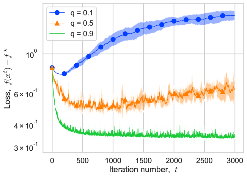
(a) Standard loss (1) convergence for different $q=K/d$.

(b) Test accuracy for different $q=K/d$.

Figure 1: Performance of Double Sketched Gradient Descent (Algorithm 1 (I)) with Rand-$K$ sketch.

In our experiments, we mainly investigate the efficacy of Double Sketched Gradient Descent (Algorithm 1 (I)) with Rand-$K$ sketches. The step size choice was informed by our theory according to Theorem 2. Figure 1 presents the averaged (over 5 runs) results (along with shaded standard deviation) due to the randomness of the method.

Standard (ERM) loss trajectory.

Figure 1(a) shows the trajectory of the train loss function for varied sparsification levels of Rand-$K$, parameterized by $q=K/d$. The findings suggest that Algorithm 1 (I) may be unsuitable for solving the conventional problem formulation (1), echoing our theoretical motivation. Moreover, higher sparsity leads to slower convergence (for low sparsity $q=0.9$) and even divergence (e.g., $q\in\{0.5,0.1\}$) after an initial short decrease of the loss. Remarkably, smaller $q$ leads to higher variance despite decreasing the step size proportionally to $q^{2}$.

Final test accuracy and sparsity.

Figure 1(b) displays the effect of the sparsification parameter $q$ on test accuracy. After running the methods for 3000 iterations, the resulting model weights were used for predictions. We observe that the performance of the method is improved significantly by reducing sparsity (increasing $q$), and accuracy matches Gradient Descent ($\mathsf{GD}$) for $q$ less than 0.4. Notably, the obtained results illustrate our method can be significantly more computationally efficient as, at every iteration, it operates with a submodel half the size of the original one. In some cases, Algorithm 1 (I) even outperforms $\mathsf{GD}$, which confirms the regularization effect of the proposed problem formulation (2) akin to the Dropout mechanism.

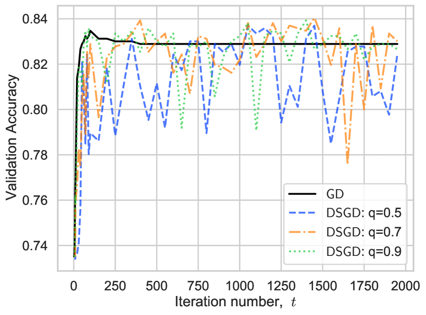
(a) Validation accuracy of Gradient Descent ($\mathsf{GD}$) and Double Sketched Gradient Descent ($\mathsf{DSGD}$).

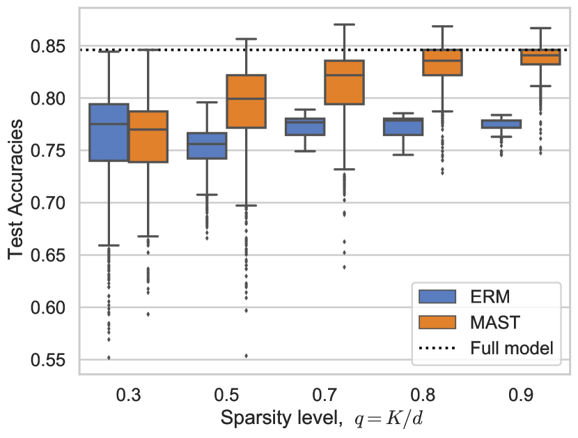
(b) Test accuracies distributions of sparsified solutions for standard (ERM) formulation (1) and MAST problem (2).

Figure 2: Validation and test performance of models based on ERM and MAST (with Rand-$K$ sketches) approaches for different $q=K/d$.

Validation accuracy trajectory.

In Figure 2(a), we compare the validation accuracy of models trained with Gradient Descent ($\mathsf{GD}$) and Double Sketched Gradient Descent (Algorithm 1 (I)) with Rand-$K$ sketch for varied sparsification parameter $q=K/d$. $\mathsf{GD}$ requires around 1500 iterations to solve the problem (drive the gradient norm on train data below $10^{-30}$) and reaches validation accuracy plateau quickly (after around 400 iterations). At the same time, the performance of $\mathsf{DSGD}$ significantly oscillates and with greater variations for higher sparsity levels (lower $q$ values). Wherein validation accuracy of $\mathsf{DSGD}$ surpasses simple $\mathsf{GD}$ at some iterations. This effect is consistent across different parameter values of $q$.

Final test accuracies distributions.

In the subsequent experiment displayed in Figure 2(b), we compare the test accuracy of sparsified solutions for standard (ERM) problem (1) and introduced MAST formulation (2). Visualization is performed using boxplot method from Seaborn (version 0.11.0) library (Waskom, 2021) with default parameters. For ERM, we find the exact (up to machine precision) optimum with $\mathsf{GD}$, subsequently used for the accuracy evaluation. For the MAST optimization problem, we use an approximate solution obtained by running $\mathsf{DSGD}$ on train data with a fixed budget of 2000 iterations for constant step size selected according to Theorem (2). The model for each sparsification level is determined based on the peak validation performance achieved after a certain number of iterations. After the ERM and MAST models ($x^{T}$) are obtained, we sample 1000 random sparsification sketches, apply them to model weights, and evaluate the test accuracy of sparsified solutions (${\bf S}x^{T}$). Figure 2(b) reveals that models obtained using the MAST approach exhibit greater robustness to random pruning compared to their ERM counterparts given the same sparsity. While ERM models show less accuracy variability, the MAST models’ median test accuracies are markedly higher. Reducing the sparsity level (greater $q$) enhances the effectiveness of the MAST models more noticeably than for ERM. In some instances, the sparsified MAST models’ accuracy surpasses that of the full ERM models, as indicated by the dotted line in the figure. These results are consistent across various levels of sparsification, with the exception of the most aggressive setting at $q=0.3$. Here, the ERM models demonstrate greater variability in performance, with a median accuracy slightly superior to that of the MAST models.

7 Conclusions and future work

In this work, a novel theoretical framework for sketched model learning was introduced. We rigorously formalized a new optimization paradigm that captures practical scenarios like Dropout and Sparse training. Efficient optimization algorithms tailored to the proposed formulation were developed and analyzed in multiple settings. Furthermore, we expanded this methodology to distributed environments, encompassing areas like IST and Federated Learning, underscoring its broad applicability.

In the future, it would be interesting to expand the class of linear matrix sketches to encompass other compression techniques, particularly those exhibiting conic variance property (contractive compressors). Such an extension might offer insights into methods like (magnitude-based) pruning and quantized training. Nevertheless, a potential challenge to be considered is the non-differentiability of such compression techniques.

Appendix

Contents

1. 1 Introduction
   1. 1.1 Motivating examples
   2. 1.2 Contributions
2. 2 Sketches
   1. 2.1 Diagonal sketches
3. 3 Problem properties
4. 4 Individual node setting
   1. 4.1 (Stochastic) Inexact Gradient
   2. 4.2 Variance Reduction
   3. 4.3 Related works discussion
5. 5 Distributed setting
   1. 5.1 Related works discussion
6. 6 Experiments
7. 7 Conclusions and future work
8. A Basic facts
9. B Auxiliary facts about functions $f_{\mathcal{D}}(x)$ and $f_{{\bf S}}(x)$
   1. B.1 Consequences of $L_{f}$-smoothness
   2. B.2 Consequences of convexity
   3. B.3 Consequences of $\mu_{f}$-convexity
10. C Relation between minima of $f$ and $f_{\mathcal{D}}$.
    1. C.1 Consequences of Lipschitz continuity of the gradient
11. D Double Sketched $\mathsf{GD}$
    1. D.1 Nonconvex analysis: Proof of Theorem 3
    2. D.2 Strongly convex analysis: Proof of Theorem 2
    3. D.3 Convex analysis
12. E (Stochastic) Inexact Gradient
    1. E.1 Nonconvex analysis: Proof of Theorem 4
    2. E.2 Strongly convex analyis
    3. E.3 Convex analyis
13. F Distributed setting
    1. F.1 Nonconvex analysis: Proof of Theorem 6
    2. F.2 Strongly convex analysis
    3. F.3 Convex analysis
14. G Variance Reduction
    1. G.1 $\mathsf{L}$-$\mathsf{SVRDSG}$: Proof of Theorem 5
       1. G.1.1 Convex analysis
    2. G.2 $\mathsf{S}$-$\mathsf{PAGE}$: Nonconvex analysis
15. H Additional experiments and details
    1. H.1 Experimental details
    2. H.2 Additional experiments

Appendix A Basic facts

For all $a,b\in\mathbb{R}^{d}$ and $\alpha>0,p\in(0,1]$ the following relations hold:

$$2\langle a,b\rangle =\|a\|^{2}+\|b\|^{2}-\|a-b\|^{2}$$ (22)

$$\|a+b\|^{2} \leq(1+\alpha)\|a\|^{2}+\left(1+\alpha^{-1}\right)\|b\|^{2}$$ (23)

$$-\|a-b\|^{2} \leq-\frac{1}{1+\alpha}\|a\|^{2}+\frac{1}{\alpha}\|b\|^{2},$$ (24)

$$(1-p)\left(1+\frac{p}{2}\right) \leq 1-\frac{p}{2},\quad p\geq 0.$$ (25)

Lemma 5 (Lemma 1 from Mishchenko et al. (2020)).

Let $X_{1},\ldots,X_{n}\in\mathbb{R}^{d}$ be fixed vectors, $\overline{X}\stackrel{{\scriptstyle\text{ def }}}{{=}}\frac{1}{n}\sum_{i=1}^{n}X_{i}$ be their average. Fix any $k\in\{1,\ldots,n\}$, let $X_{\pi_{1}},\ldots X_{\pi_{k}}$ be sampled uniformly without replacement from $\left\{X_{1},\ldots,X_{n}\right\}$ and $\overline{X}_{\pi}$ be their average. Then, the sample average and variance are given by

$$\mathbb{E}\left[\overline{X}_{\pi}\right]=\overline{X}$$

$$\mathbb{E}\left[\left\|\overline{X}_{\pi}-\overline{X}\right\|^{2}\right]=\frac{n-k}{k(n-1)}\frac{1}{n}\sum_{i=1}^{n}\left\|X_{i}-\overline{X}\right\|^{2}$$

Lemma 6.

(Lemma 5 from Richtárik et al. (2021)). Let $a,b>0$. If $0\leq\gamma\leq\frac{1}{\sqrt{a}+b}$, then $a\gamma^{2}+b\gamma\leq 1$. The bound is tight up to the factor of 2 since $\frac{1}{\sqrt{a}+b}\leq\min\left\{\frac{1}{\sqrt{a}},\frac{1}{b}\right\}\leq\frac{2}{\sqrt{a}+b}$.

Proposition 1.

Nonzero eigenvalues of $\;{\bf S}{\bf S}^{\top}$ and $\;{\bf S}^{\top}{\bf S}$ coincide.

Proof.

Indeed, suppose $\lambda\neq 0$ is an eigenvalue of ${\bf S}^{\top}{\bf S}$ with an eigenvector $v\in\mathbb{R}^{d},$ then $\lambda$ is an eigenvalue of ${\bf S}{\bf S}^{\top}$ with an eigenvector ${\bf S}v.$ ∎

Lemma 7.

Suppose that $f(x)$ is $L_{f}$-smooth, differentiable and bounded from below by $f^{\inf}.$ Then

$$\left\|\nabla f(x)\right\|^{2}\leq 2L_{f}\left(f(x)-f^{\inf}\right),\quad\forall x\in\mathbb{R}^{d}.$$ (26)

Proof.

Let $x^{+}=x-\frac{1}{L_{f}}\nabla f(x),$ then using the $L_{f}$-smoothness of $f$ we obtain

$$f(x^{+})\leq f(x)+\langle\nabla f(x),x^{+}-x\rangle+\frac{L_{f}}{2}\left\|x^{+}-x\right\|^{2}.$$

Since $f^{\inf}\leq f(x^{+})$ and the definition of $x^{+}$ we have,

$$f^{\inf}\leq f(x^{+})\leq f(x)-\frac{1}{L_{f}}\left\|\nabla f(x)\right\|^{2}+\frac{1}{2L_{f}}\left\|\nabla f(x)\right\|^{2}=f(x)-\frac{1}{2L_{f}}\left\|\nabla f(x)\right\|^{2}.$$

It remains to rearrange the terms to get the claimed result. ∎

Appendix B Auxiliary facts about functions $f_{\mathcal{D}}(x)$ and $f_{{\bf S}}(x)$

For a differentiable function $f:\mathbb{R}^{d}\to\mathbb{R}$ and $x,y\in\mathbb{R}^{d},$ Bregman divergence associated with $f$ is $D_{f}(x,y)\stackrel{{\scriptstyle\text{def}}}{{=}}f(x)-f(y)-\langle\nabla f(y),x-y\rangle.$

Lemma 8 (Bregman divergence).

If $f$ is continuously differentiable, then $D_{f_{\mathcal{D}}}(x,y)={\mathbb{E}}\left[D_{f_{{\bf S}}}(x,y)\right].$

Proof.

Since $f$ is continuously differentiable, we can interchange integration and differentiation. The result follows from the linearity of expectation. ∎

B.1 Consequences of $L_{f}$-smoothness

Recall the $L_{f}$-smoothness assumption.
Assumption 2. Function $f$ is differentiable and $L_{f}$-smooth, i.e., there is $L_{f}>0$ such that $\forall x,h\in\mathbb{R}^{d}$

$$f(x+h)\leq f(x)+\left\langle\nabla f(x),h\right\rangle+\frac{L_{f}}{2}\left\|h\right\|^{2}.$$

We also require $f$ to be lower bounded by $f^{\inf}\in\mathbb{R}$.

Lemma 9 (Consequences of $L_{f}$-smoothness).

If $f$ is $L_{f}$-smooth, then

• $f_{{\bf S}}$ is $L_{f_{\bf S}}$-smooth with $L_{f_{\bf S}}\leq L_{{\bf S}}L_{f}.$ That is,

  $$f_{{\bf S}}(x+h)\leq f_{{\bf S}}(x)+\left\langle\nabla f_{{\bf S}}(x),h\right\rangle+\frac{L_{{\bf S}}L_{f}}{2}\left\|h\right\|^{2},\quad\forall x,h\in\mathbb{R}^{d}.$$

• $f_{\mathcal{D}}$ is $L_{f_{\mathcal{D}}}$-smooth with $L_{f_{\mathcal{D}}}\leq L_{\mathcal{D}}L_{f}.$ That is,

  $$f_{\mathcal{D}}(x+h)\leq f_{\mathcal{D}}(x)+\left\langle\nabla f_{\mathcal{D}}(x),h\right\rangle+\frac{L_{\mathcal{D}}L_{f}}{2}\left\|h\right\|^{2},\quad\forall x,h\in\mathbb{R}^{d}.$$

• $$f_{\mathcal{D}}(x)\leq f(x)+\frac{(L_{\mathcal{D}}-1)L_{f}}{2}\left\|x-{\color[rgb]{.75,0,.25}v}\right\|^{2},\quad\forall x\in\mathbb{R}^{d}.$$ (27)

Proof.

• For any $x,h\in\mathbb{R}^{d}$, we have

  $$f_{{\bf S}}(x+h) = f({\color[rgb]{.75,0,.25}v}+{\bf S}(x+h-{\color[rgb]{.75,0,.25}v}))$$

  $$= f({\color[rgb]{.75,0,.25}v}+{\bf S}(x-{\color[rgb]{.75,0,.25}v})+{\bf S}h)$$

  $$\stackrel{{\scriptstyle\mathrm{Asn.}~{}\ref{ass:l_f_smooth}}}{{\leq}} f({\color[rgb]{.75,0,.25}v}+{\bf S}(x-{\color[rgb]{.75,0,.25}v}))+\left\langle\nabla f({\color[rgb]{.75,0,.25}v}+{\bf S}(x-{\color[rgb]{.75,0,.25}v})),{\bf S}h\right\rangle+\frac{L_{f}}{2}\left\|{\bf S}h\right\|^{2}$$

  $$= f({\color[rgb]{.75,0,.25}v}+{\bf S}(x-{\color[rgb]{.75,0,.25}v}))+\left\langle{\bf S}^{\top}\nabla f({\color[rgb]{.75,0,.25}v}+{\bf S}(x-{\color[rgb]{.75,0,.25}v})),h\right\rangle+\frac{L_{f}}{2}\left\langle{\bf S}^{\top}{\bf S}h,h\right\rangle$$

  $$\leq f_{{\bf S}}(x)+\left\langle\nabla f_{{\bf S}}(x),h\right\rangle+\frac{L_{{\bf S}}L_{f}}{2}\left\|h\right\|^{2}.$$

• For any $x,h\in\mathbb{R}^{d}$, we have

  $$f_{\mathcal{D}}(x+h) = {\mathbb{E}}\left[f({\color[rgb]{.75,0,.25}v}+{\bf S}(x+h-{\color[rgb]{.75,0,.25}v}))\right]$$

  $$= {\mathbb{E}}\left[f({\color[rgb]{.75,0,.25}v}+{\bf S}(x-{\color[rgb]{.75,0,.25}v})+{\bf S}h)\right]$$

  $$\stackrel{{\scriptstyle\mathrm{Asn.}~{}\ref{ass:l_f_smooth}}}{{\leq}} {\mathbb{E}}\left[f({\color[rgb]{.75,0,.25}v}+{\bf S}(x-{\color[rgb]{.75,0,.25}v}))+\left\langle\nabla f({\color[rgb]{.75,0,.25}v}+{\bf S}(x-{\color[rgb]{.75,0,.25}v})),{\bf S}h\right\rangle+\frac{L_{f}}{2}\left\|{\bf S}h\right\|^{2}\right]$$

  $$= {\mathbb{E}}\left[f({\color[rgb]{.75,0,.25}v}+{\bf S}(x-{\color[rgb]{.75,0,.25}v}))\right]+\left\langle{\mathbb{E}}\left[{\bf S}^{\top}\nabla f({\color[rgb]{.75,0,.25}v}+{\bf S}(x-{\color[rgb]{.75,0,.25}v}))\right],h\right\rangle+\frac{L_{f}}{2}{\mathbb{E}}\left[\left\|{\bf S}h\right\|^{2}\right]$$

  $$= f_{\mathcal{D}}(x)+\left\langle\nabla f_{\mathcal{D}}(x),h\right\rangle+\frac{L_{f}}{2}\left\langle{\mathbb{E}}\left[{\bf S}^{\top}{\bf S}\right]h,h\right\rangle$$

  $$\leq f_{\mathcal{D}}(x)+\left\langle\nabla f_{\mathcal{D}}(x),h\right\rangle+\frac{L_{\mathcal{D}}L_{f}}{2}\left\|h\right\|^{2}.$$

• For any $x\in\mathbb{R}^{d}$, we have

  $$f_{\mathcal{D}}(x) = {\mathbb{E}}\left[f({\color[rgb]{.75,0,.25}v}+{\bf S}(x-{\color[rgb]{.75,0,.25}v}))\right]$$

  $$\stackrel{{\scriptstyle\mathrm{Asn.}~{}\ref{ass:l_f_smooth}}}{{\leq}} {\mathbb{E}}\left[f(x)+\left\langle\nabla f(x),{\bf S}(x-{\color[rgb]{.75,0,.25}v})-(x-{\color[rgb]{.75,0,.25}v})\right\rangle+\frac{L_{f}}{2}\left\|{\bf S}(x-{\color[rgb]{.75,0,.25}v})-(x-{\color[rgb]{.75,0,.25}v})\right\|^{2}\right]$$

  $$= f(x)+\left\langle\nabla f(x),{\mathbb{E}}\left[{\bf S}(x-{\color[rgb]{.75,0,.25}v})-(x-{\color[rgb]{.75,0,.25}v})\right]\right\rangle+\frac{L_{f}}{2}{\mathbb{E}}\left[\left\|{\bf S}(x-{\color[rgb]{.75,0,.25}v})-(x-{\color[rgb]{.75,0,.25}v})\right\|^{2}\right]$$

  $$\overset{\eqref{eq:sketch_def}}{=} f(x)+\left\langle\nabla f(x),0\right\rangle+\frac{L_{f}}{2}(x-{\color[rgb]{.75,0,.25}v})^{\top}\left({\mathbb{E}}\left[{\bf S}^{\top}{\bf S}\right]-\mathbf{I}\right)(x-{\color[rgb]{.75,0,.25}v})$$

  $$= f(x)+\frac{(L_{\mathcal{D}}-1)L_{f}}{2}\left\|x-{\color[rgb]{.75,0,.25}v}\right\|^{2}.$$

∎

B.2 Consequences of convexity

We do not assume differentiability of $f$ here. Recall that function $f$ is convex if, for all $x,y\in\mathbb{R}^{d}$ and $\alpha\in[0,1],$ we have that $f(\alpha x+(1-\alpha)y)\leq\alpha f(x)+(1-\alpha)f(y).$

Lemma 10.

If $f$ is convex, then $f_{\mathcal{D}}$ is convex and $f_{\mathcal{D}}(x)\geq f(x)$ for all $x\in\mathbb{R}^{d}$.

Proof.

• Let $x,y\in\mathbb{R}^{d}$ and $\alpha\in[0,1]$. Then

  $$f_{\mathcal{D}}(\alpha x+(1-\alpha)y) \overset{\eqref{eq:pretrained_compressed_problem}}{=} {\mathbb{E}}\left[f({\color[rgb]{.75,0,.25}v}+{\bf S}(\alpha x+(1-\alpha)y-{\color[rgb]{.75,0,.25}v}))\right]$$

  $$= {\mathbb{E}}\left[f(\alpha\left({\color[rgb]{.75,0,.25}v}+{\bf S}(x-{\color[rgb]{.75,0,.25}v})\right)+(1-\alpha)\left({\color[rgb]{.75,0,.25}v}+{\bf S}(y-{\color[rgb]{.75,0,.25}v})\right))\right]$$

  $$\leq {\mathbb{E}}\left[\alpha f({\color[rgb]{.75,0,.25}v}+{\bf S}(x-{\color[rgb]{.75,0,.25}v}))+(1-\alpha)f({\color[rgb]{.75,0,.25}v}+{\bf S}(y-{\color[rgb]{.75,0,.25}v}))\right]$$

  $$= \alpha{\mathbb{E}}\left[f({\color[rgb]{.75,0,.25}v}+{\bf S}(x-{\color[rgb]{.75,0,.25}v}))\right]+(1-\alpha){\mathbb{E}}\left[f({\color[rgb]{.75,0,.25}v}+{\bf S}(y-{\color[rgb]{.75,0,.25}v}))\right]$$

  $$\overset{\eqref{eq:pretrained_compressed_problem}}{=} \alpha f_{\mathcal{D}}(x)+(1-\alpha)f_{\mathcal{D}}(y).$$

  Alternative proof: Each $f_{{\bf S}}$ is obviously convex, and expectation of convex functions is a convex function.

• Fix $x\in\mathbb{R}^{d}$ and let $g\in\partial f(x)$ be a subgradient of $f$ at $x$. Then

  $$f_{\mathcal{D}}(x) \overset{\eqref{eq:pretrained_compressed_problem}}{=} {\mathbb{E}}\left[f({\color[rgb]{.75,0,.25}v}+{\bf S}(x-{\color[rgb]{.75,0,.25}v}))\right]$$

  $$\geq {\mathbb{E}}\left[f(x)+\left\langle g,{\bf S}(x-{\color[rgb]{.75,0,.25}v})-(x-{\color[rgb]{.75,0,.25}v})\right\rangle\right]$$

  $$= f(x)+\left\langle g,{\mathbb{E}}\left[{\bf S}(x-{\color[rgb]{.75,0,.25}v})-(x-{\color[rgb]{.75,0,.25}v})\right]\right\rangle$$

  $$\overset{\eqref{eq:sketch_def}}{=} f(x)+\left\langle g,0\right\rangle$$

  $$= f(x).$$

  Alternative proof: Using Jensen’s inequality, $f({\color[rgb]{.75,0,.25}v}+{\bf S}(x-{\color[rgb]{.75,0,.25}v}))={\mathbb{E}}\left[{\color[rgb]{.75,0,.25}v}+{\bf S}(x-{\color[rgb]{.75,0,.25}v})\right]\geq f({\mathbb{E}}\left[{\color[rgb]{.75,0,.25}v}+{\bf S}(x-{\color[rgb]{.75,0,.25}v})\right])=f(x)$.

∎

B.3 Consequences of $\mu_{f}$-convexity

Recall the $\mu_{f}$-strong convexity (or, for simplicity, $\mu_{f}$-convexity) assumption.
Assumption 3. Function $f$ is differentiable and $\mu_{f}$-strongly convex, i.e., there is $\mu_{f}>0$ such that $\forall x,h\in\mathbb{R}^{d}$

$$f(x+h)\geq f(x)+\left\langle\nabla f(x),h\right\rangle+\frac{\mu_{f}}{2}\left\|h\right\|^{2}.$$

Lemma 11 (Consequences of $\mu_{f}$-convexity).

If $f$ is $\mu_{f}$-convex, then

• $f_{{\bf S}}$ is $\mu_{f_{\bf S}}$-convex with $\mu_{f_{\bf S}}\geq\mu_{{\bf S}}\mu_{f}.$ That is,

  $$f_{{\bf S}}(x+h)\geq f_{{\bf S}}(x)+\left\langle\nabla f_{{\bf S}}(x),h\right\rangle+\frac{\mu_{{\bf S}}\mu_{f}}{2}\left\|h\right\|^{2},\quad\forall x,h\in\mathbb{R}^{d}.$$

• $f_{\mathcal{D}}$ is $\mu_{f_{\mathcal{D}}}$-convex with $\mu_{f_{\mathcal{D}}}\geq\mu_{\mathcal{D}}\mu_{f}.$ That is,

  $$f_{\mathcal{D}}(x+h)\geq f_{\mathcal{D}}(x)+\left\langle\nabla f_{\mathcal{D}}(x),h\right\rangle+\frac{\mu_{\mathcal{D}}\mu_{f}}{2}\left\|h\right\|^{2},\quad\forall x,h\in\mathbb{R}^{d}.$$

• $$f_{\mathcal{D}}(x)\geq f(x)+\frac{(\mu_{\mathcal{D}}-1)\mu_{f}}{2}\left\|x-{\color[rgb]{.75,0,.25}v}\right\|^{2},\quad\forall x\in\mathbb{R}^{d}.$$ (28)

Proof.

• For any $x,h\in\mathbb{R}^{d}$, we have

  $$f_{{\bf S}}(x+h) = f({\color[rgb]{.75,0,.25}v}+{\bf S}(x+h-{\color[rgb]{.75,0,.25}v}))$$

  $$= f({\color[rgb]{.75,0,.25}v}+{\bf S}(x-{\color[rgb]{.75,0,.25}v})+{\bf S}h)$$

  $$\stackrel{{\scriptstyle\mathrm{Asn.}~{}\ref{ass:mu_f-convex}}}{{\geq}} f({\color[rgb]{.75,0,.25}v}+{\bf S}(x-{\color[rgb]{.75,0,.25}v}))+\left\langle\nabla f({\color[rgb]{.75,0,.25}v}+{\bf S}(x-{\color[rgb]{.75,0,.25}v})),{\bf S}h\right\rangle+\frac{\mu_{f}}{2}\left\|{\bf S}h\right\|^{2}$$

  $$= f({\color[rgb]{.75,0,.25}v}+{\bf S}(x-{\color[rgb]{.75,0,.25}v}))+\left\langle{\bf S}^{\top}\nabla f({\color[rgb]{.75,0,.25}v}+{\bf S}(x-{\color[rgb]{.75,0,.25}v})),h\right\rangle+\frac{\mu_{f}}{2}\left\langle{\bf S}^{\top}{\bf S}h,h\right\rangle$$

  $$\geq f_{{\bf S}}(x)+\left\langle\nabla f_{{\bf S}}(x),h\right\rangle+\frac{\mu_{{\bf S}}\mu_{f}}{2}\left\|h\right\|^{2}.$$

• For any $x,h\in\mathbb{R}^{d}$, we have

  $$f_{\mathcal{D}}(x+h) = {\mathbb{E}}\left[f({\color[rgb]{.75,0,.25}v}+{\bf S}(x+h-{\color[rgb]{.75,0,.25}v}))\right]$$

  $$= {\mathbb{E}}\left[f({\color[rgb]{.75,0,.25}v}+{\bf S}(x-{\color[rgb]{.75,0,.25}v})+{\bf S}h)\right]$$

  $$\stackrel{{\scriptstyle\mathrm{Asn.}~{}\ref{ass:mu_f-convex}}}{{\geq}} {\mathbb{E}}\left[f({\color[rgb]{.75,0,.25}v}+{\bf S}(x-{\color[rgb]{.75,0,.25}v}))+\left\langle\nabla f({\color[rgb]{.75,0,.25}v}+{\bf S}(x-{\color[rgb]{.75,0,.25}v})),{\bf S}h\right\rangle+\frac{\mu_{f}}{2}\left\|{\bf S}h\right\|^{2}\right]$$

  $$= {\mathbb{E}}\left[f({\color[rgb]{.75,0,.25}v}+{\bf S}(x-{\color[rgb]{.75,0,.25}v}))\right]+\left\langle{\mathbb{E}}\left[{\bf S}^{\top}\nabla f({\color[rgb]{.75,0,.25}v}+{\bf S}(x-{\color[rgb]{.75,0,.25}v}))\right],h\right\rangle+\frac{\mu_{f}}{2}{\mathbb{E}}\left[\left\|{\bf S}h\right\|^{2}\right]$$

  $$= f_{\mathcal{D}}(x)+\left\langle\nabla f_{\mathcal{D}}(x),h\right\rangle+\frac{\mu_{f}}{2}\left\langle{\mathbb{E}}\left[{\bf S}^{\top}{\bf S}\right]h,h\right\rangle$$

  $$\geq f_{\mathcal{D}}(x)+\left\langle\nabla f_{\mathcal{D}}(x),h\right\rangle+\frac{\mu_{\mathcal{D}}\mu_{f}}{2}\left\|h\right\|^{2}.$$

• For any $x\in\mathbb{R}^{d}$, we have

  $$f_{\mathcal{D}}(x) = {\mathbb{E}}\left[f({\color[rgb]{.75,0,.25}v}+{\bf S}(x-{\color[rgb]{.75,0,.25}v}))\right]$$

  $$\stackrel{{\scriptstyle\mathrm{Asn.}~{}\ref{ass:mu_f-convex}}}{{\geq}} {\mathbb{E}}\left[f(x)+\left\langle\nabla f(x),{\bf S}(x-{\color[rgb]{.75,0,.25}v})-(x-{\color[rgb]{.75,0,.25}v})\right\rangle+\frac{\mu_{f}}{2}\left\|{\bf S}(x-{\color[rgb]{.75,0,.25}v})-(x-{\color[rgb]{.75,0,.25}v})\right\|^{2}\right]$$

  $$= f(x)+\left\langle\nabla f(x),{\mathbb{E}}\left[{\bf S}(x-{\color[rgb]{.75,0,.25}v})-(x-{\color[rgb]{.75,0,.25}v})\right]\right\rangle+\frac{\mu_{f}}{2}{\mathbb{E}}\left[\left\|{\bf S}(x-{\color[rgb]{.75,0,.25}v})-(x-{\color[rgb]{.75,0,.25}v})\right\|^{2}\right]$$

  $$\overset{\eqref{eq:sketch_def}}{=} f(x)+\left\langle\nabla f(x),0\right\rangle+\frac{\mu_{f}}{2}(x-{\color[rgb]{.75,0,.25}v})^{\top}\left({\mathbb{E}}\left[{\bf S}^{\top}{\bf S}\right]-\mathbf{I}\right)(x-{\color[rgb]{.75,0,.25}v})$$

  $$= f(x)+\frac{(\mu_{\mathcal{D}}-1)\mu_{f}}{2}\left\|x-{\color[rgb]{.75,0,.25}v}\right\|^{2}.$$

∎

Appendix C Relation between minima of $f$ and $f_{\mathcal{D}}$.

Theorem 7.

Let Assumptions 2 and 3 hold, and let $x_{\mathcal{D}}^{\star}\in\tilde{{\cal X}}$ and $x^{\star}\in{\cal X}^{\star}$. Then

$$f(x^{\star})\leq f(x_{\mathcal{D}}^{\star})\leq f(x^{\star})+\frac{(L_{\mathcal{D}}-1)L_{f}}{2}\left\|x^{\star}-{\color[rgb]{.75,0,.25}v}\right\|^{2}-\frac{(\mu_{\mathcal{D}}-1)\mu_{f}}{2}\left\|x_{\mathcal{D}}^{\star}-{\color[rgb]{.75,0,.25}v}\right\|^{2}.$$

Proof.

The result follows by combining inequalities (27) and (28):

$$\begin{split}f(x_{\mathcal{D}}^{\star})+\frac{(\mu_{\mathcal{D}}-1)\mu_{f}}{2}\left\|x_{\mathcal{D}}^{\star}-{\color[rgb]{.75,0,.25}v}\right\|^{2}\overset{\eqref{eq:mu_f-convex-iii_appendix}}{\leq}f_{\mathcal{D}}(x_{\mathcal{D}}^{\star})\leq f_{\mathcal{D}}(x^{\star})\overset{\eqref{eq:L_f-smooth-iii_appendix}}{\leq}f(x^{\star})+\frac{(L_{\mathcal{D}}-1)L_{f}}{2}\left\|x^{\star}-{\color[rgb]{.75,0,.25}v}\right\|^{2}.\end{split}$$

∎

C.1 Consequences of Lipschitz continuity of the gradient

Gradient of $f(x)$ is $L_{f}$-Lipschitz if, for all $x,y\in\mathbb{R}^{d},$ we have that $\left\|\nabla f(x)-\nabla f(y)\right\|\leq L_{f}\left\|x-y\right\|.$

Lemma 12.

If $\nabla f$ is $L_{f}$-Lipschitz, then $\nabla f_{\mathcal{D}}$ is $L_{f_{\mathcal{D}}}$-Lipschitz with

$$L_{f_{\mathcal{D}}}\leq L_{f}{\mathbb{E}}\left[\left\|{\bf S}^{\top}\right\|\left\|{\bf S}\right\|\right].$$

Proof.

We have that

$$\left\|\nabla f_{\mathcal{D}}(x)-\nabla f_{\mathcal{D}}(y)\right\| = \left\|\nabla{\mathbb{E}}\left[f({\color[rgb]{.75,0,.25}v}+{\bf S}(x-{\color[rgb]{.75,0,.25}v}))\right]-\nabla{\mathbb{E}}\left[f({\color[rgb]{.75,0,.25}v}+{\bf S}(y-{\color[rgb]{.75,0,.25}v}))\right]\right\|$$

$$= \left\|{\mathbb{E}}\left[{\bf S}^{\top}\nabla f({\color[rgb]{.75,0,.25}v}+{\bf S}(x-{\color[rgb]{.75,0,.25}v}))\right]-{\mathbb{E}}\left[{\bf S}^{\top}\nabla f({\color[rgb]{.75,0,.25}v}+{\bf S}(y-{\color[rgb]{.75,0,.25}v}))\right]\right\|$$

$$= \left\|{\mathbb{E}}\left[{\bf S}^{\top}\nabla f({\color[rgb]{.75,0,.25}v}+{\bf S}(x-{\color[rgb]{.75,0,.25}v}))-{\bf S}^{\top}\nabla f({\color[rgb]{.75,0,.25}v}+{\bf S}(y-{\color[rgb]{.75,0,.25}v}))\right]\right\|$$

$$\leq {\mathbb{E}}\left[\left\|{\bf S}^{\top}\nabla f({\color[rgb]{.75,0,.25}v}+{\bf S}(x-{\color[rgb]{.75,0,.25}v}))-{\bf S}^{\top}\nabla f({\color[rgb]{.75,0,.25}v}+{\bf S}(y-{\color[rgb]{.75,0,.25}v}))\right\|\right]$$

$$\leq {\mathbb{E}}\left[\left\|{\bf S}^{\top}\right\|\left\|\nabla f({\color[rgb]{.75,0,.25}v}+{\bf S}(x-{\color[rgb]{.75,0,.25}v}))-\nabla f({\color[rgb]{.75,0,.25}v}+{\bf S}(y-{\color[rgb]{.75,0,.25}v}))\right\|\right]$$

$$\leq {\mathbb{E}}\left[\left\|{\bf S}^{\top}\right\|L_{f}\left\|{\bf S}x-{\bf S}y\right\|\right]$$

$$\leq L_{f}{\mathbb{E}}\left[\left\|{\bf S}^{\top}\right\|\left\|{\bf S}\right\|\right]\left\|x-y\right\|.$$

∎

Appendix D Double Sketched $\mathsf{GD}$

Recall that $L_{{\bf S}}^{\max}=\sup_{{\bf S}}\left\{\lambda_{\max}\left({\bf S}^{\top}{\bf S}\right)\right\}=\sup_{{\bf S}}\left\{\lambda_{\max}\left({\bf S}{\bf S}^{\top}\right)\right\}$ (we used Proposition 1).

D.1 Nonconvex analysis: Proof of Theorem 3

Lemma 13.

For all $x\in\mathbb{R}^{d},$ we have that

$$\begin{split}{\mathbb{E}}\left[\left\|\nabla f_{{\bf S}}(x)\right\|^{2}\right]&\leq 2L_{f}L_{{\bf S}}^{\max}\left(f_{\mathcal{D}}(x)-f^{\inf}\right).\\ \end{split}$$

where the expectation is taken with respect to ${\bf S}.$

Proof.

Due to $L_{f}$-smoothness of $f,$ we have that

$$\begin{split}{\mathbb{E}}\left[\left\|\nabla f_{{\bf S}}(x)\right\|^{2}\right]&={\mathbb{E}}\left[\left\|{\bf S}^{\top}\nabla f(y)|_{y=s+{\bf S}(x-s)}\right\|^{2}\right]\\ &={\mathbb{E}}\left[\left\langle{\bf S}^{\top}\nabla f(y),{\bf S}^{\top}\nabla f(y)\right\rangle|_{y=s+{\bf S}(x-s)}\right]\\ &={\mathbb{E}}\left[\left\langle{\bf S}{\bf S}^{\top}\nabla f(y),\nabla f(y)\right\rangle|_{y=s+{\bf S}(x-s)}\right]\\ &\leq{\mathbb{E}}\left[\lambda_{\max}\left({\bf S}{\bf S}^{\top}\right)\left\|\nabla f(y)|_{y=s+{\bf S}(x-s)}\right\|^{2}\right]\\ &\leq L_{{\bf S}}^{\max}{\mathbb{E}}\left[\left\|\nabla f(y)|_{y=s+{\bf S}(x-s)}\right\|^{2}\right]\\ &\stackrel{{\scriptstyle\eqref{eq:smoothness_bregman}}}{{\leq}}2L_{f}L_{{\bf S}}^{\max}{\mathbb{E}}\left[f\left(s+{\bf S}(x-s)\right)-f^{\inf}\right]\\ &=2L_{f}L_{{\bf S}}^{\max}\left(f_{\mathcal{D}}(x)-f^{\inf}\right).\\ \end{split}$$

∎

All convergence results in the nonconvex scenarios rely on the following key lemma.

Lemma 14.

The iterates $\{x^{t}\}_{t\geq 0}$ of $\mathsf{SGD}$ satisfy

$$\begin{split}\gamma r^{t}\leq\left(1+\gamma^{2}M_{1}\right)\delta^{t}-\delta^{t+1}+\gamma^{2}M_{2},\end{split}$$ (29)

where $M_{1}$ and $M_{2}$ are non-negative constants, $\delta^{t}\stackrel{{\scriptstyle\text{def}}}{{=}}\mathbb{E}\left[f_{\mathcal{D}}(x^{t})-f_{\mathcal{D}}^{\inf}\right]$ and $r^{t}\stackrel{{\scriptstyle\text{def}}}{{=}}\mathbb{E}\left[\left\|\nabla f_{\mathcal{D}}(x^{t})\right\|^{2}\right].$ Fix $w_{-1}>0$ and, for all $t\geq 0,$ define $w_{t}=\frac{w_{t-1}}{1+\gamma^{2}M_{1}}.$ Then, for any $T\geq 1,$ the iterates $\{x^{t}\}_{t\geq 0}$ satisfy

$$\sum_{t=0}^{T-1}w_{t}r^{t}\leq\frac{w_{1}}{\gamma}\delta^{0}-\frac{w_{T-1}}{\gamma}\delta^{T}+\gamma M_{2}\sum_{t=0}^{T-1}w_{t}.$$

Proof.

Multiplying both sides of (29) by $\frac{w_{t}}{\gamma},$ we obtain

$$w_{t}r^{t}\leq\frac{w_{t-1}}{\gamma}\delta^{t}-\frac{w_{t}}{\gamma}\delta^{t+1}+\gamma w_{t}M_{2}.$$

For every $0\leq t\leq T-1,$ sum these inequalities. We arrive at

$$\sum_{t=0}^{T-1}w_{t}r^{t}\leq\frac{w_{-1}}{\gamma}\delta^{0}-\frac{w_{T-1}}{\gamma}\delta^{T}+\gamma M_{2}\sum_{t=0}^{T-1}w_{t}.$$

∎

Recall that $D\stackrel{{\scriptstyle\text{def}}}{{=}}L_{f}\sqrt{L_{\mathcal{D}}L_{{\bf S}}^{\max}}.$

Theorem 8.

Let Assumptions 1 and 2 hold. For every $t\geq 0,$ put $\delta^{t}\stackrel{{\scriptstyle\text{def}}}{{=}}\mathbb{E}\left[f_{\mathcal{D}}(x^{t})-f_{\mathcal{D}}^{\inf}\right]$ and $r^{t}\stackrel{{\scriptstyle\text{def}}}{{=}}\mathbb{E}\left[\left\|\nabla f_{\mathcal{D}}(x^{t})\right\|^{2}\right].$ Then, for any $T\geq 1,$ the iterates $\{x^{t}\}_{t=0}^{T-1}$ of Algorithm 1 satisfy

$$\min_{0\leq t<T}r^{t}\leq\frac{\left(1+D^{2}\gamma^{2}\right)^{T}}{\gamma T}\delta^{0}+D^{2}\gamma\left(f_{\mathcal{D}}^{\inf}-f^{\inf}\right).$$ (30)

Proof.

Due to $L_{f}$-smoothness of $f,$ we have that

$$\begin{split}f(s+{\bf S}^{t+1}(x^{t+1}-s))&\leq f(s+{\bf S}^{t+1}(x^{t}-s))\\ &+\bigg{<}\nabla f\left(y\right)|_{y=s+{\bf S}^{t+1}(x^{t}-s)},{\bf S}^{t+1}\left(x^{t+1}-s\right)-{\bf S}^{t+1}\left(x^{t}-s\right)\bigg{>}\\ &+\frac{L_{f}}{2}\left\|{\bf S}^{t+1}\left(x^{t+1}-s\right)-{\bf S}^{t+1}\left(x^{t}-s\right)\right\|^{2}\\ &=f(s+{\bf S}^{t+1}(x^{t}-s))-\gamma\bigg{<}\nabla f\left(y\right)|_{y=s+{\bf S}^{t+1}(x^{t}-s)},{\bf S}^{t+1}\nabla f_{{\bf S}^{t}}(x^{t})\bigg{>}\\ &+\frac{L_{f}\gamma^{2}}{2}\left\|{\bf S}^{t+1}\nabla f_{{\bf S}^{t}}(x^{t})\right\|^{2}\\ &\leq f(s+{\bf S}^{t+1}(x^{t}-s))-\gamma\bigg{<}\nabla f_{{\bf S}^{t+1}}\left(x^{t}\right),\nabla f_{{\bf S}^{t}}(x^{t})\bigg{>}\\ &+\frac{L_{f}\gamma^{2}}{2}\bigg{<}\left({\bf S}^{t+1}\right)^{\top}{\bf S}^{t+1}\nabla f_{{\bf S}^{t}}(x^{t}),\nabla f_{{\bf S}^{t}}(x^{t})\bigg{>}.\\ \end{split}$$

Taking the expectation with respect to ${\bf S}^{t+1}$ yields

$$\begin{split}f_{\mathcal{D}}\left(x^{t+1}\right)&\leq f_{\mathcal{D}}\left(x^{t}\right)-\gamma\bigg{<}\nabla f_{\mathcal{D}}\left(x^{t}\right),\nabla f_{{\bf S}^{t}}(x^{t})\bigg{>}+\frac{L_{f}\gamma^{2}}{2}\bigg{<}{\mathbb{E}}\left[\left({\bf S}^{t+1}\right)^{\top}{\bf S}^{t+1}\right]\nabla f_{{\bf S}^{t}}(x^{t}),\nabla f_{{\bf S}^{t}}(x^{t})\bigg{>}\\ &\leq f_{\mathcal{D}}\left(x^{t}\right)-\gamma\bigg{<}\nabla f_{\mathcal{D}}\left(x^{t}\right),\nabla f_{{\bf S}^{t}}(x^{t})\bigg{>}+\frac{L_{f}L_{\mathcal{D}}\gamma^{2}}{2}\left\|\nabla f_{{\bf S}^{t}}(x^{t})\right\|^{2}.\end{split}$$

Conditioned on $x^{t},$ take expectation with respect to ${\bf S}^{t}:$

$$\begin{split}{\mathbb{E}}\left[f_{\mathcal{D}}\left(x^{t+1}\right)|x^{t}\right]\leq f_{\mathcal{D}}\left(x^{t}\right)-\gamma\left\|\nabla f_{\mathcal{D}}\left(x^{t}\right)\right\|^{2}+\frac{L_{f}L_{\mathcal{D}}\gamma^{2}}{2}{\mathbb{E}}\left[\left\|\nabla f_{{\bf S}^{t}}(x^{t})\right\|^{2}\right].\\ \end{split}$$

From Lemma 4 we obtain that

$$\begin{split}{\mathbb{E}}\left[f_{\mathcal{D}}\left(x^{t+1}\right)|x^{t}\right]&\leq f_{\mathcal{D}}\left(x^{t}\right)-\gamma\left\|\nabla f_{\mathcal{D}}\left(x^{t}\right)\right\|^{2}\\ &\qquad+\frac{L_{f}L_{\mathcal{D}}\gamma^{2}}{2}\left(2L_{f}L_{{\bf S}}^{\max}\left(f_{\mathcal{D}}(x)-f_{\mathcal{D}}^{\inf}\right)\right.+\left.2L_{f}L_{{\bf S}}^{\max}\left(f_{\mathcal{D}}^{\inf}-f^{\inf}\right)\right).\end{split}$$

Subtract $f_{\mathcal{D}}^{\inf}$ from both sides, take expectations on both sides, and use the tower property:

$$\begin{split}{\mathbb{E}}\left[f_{\mathcal{D}}\left(x^{t+1}\right)-f_{\mathcal{D}}^{\inf}\right]&\leq\left(1+D^{2}\gamma^{2}\right){\mathbb{E}}\left[f_{\mathcal{D}}\left(x^{t}\right)-f_{\mathcal{D}}^{\inf}\right]-\gamma{\mathbb{E}}\left[\left\|\nabla f_{\mathcal{D}}\left(x^{t}\right)\right\|^{2}\right]+D^{2}\gamma^{2}\left(f_{\mathcal{D}}^{\inf}-f^{\inf}\right).\\ \end{split}$$

We obtain that

$$\begin{split}\gamma r^{t}\leq\left(1+D^{2}\gamma^{2}\right)\delta^{t}-\delta^{t+1}+D\gamma^{2}\left(f_{\mathcal{D}}^{\inf}-f^{\inf}\right).\end{split}$$

Notice that the iterates $\{x^{t}\}_{t\geq 0}$ of Algorithm 1 satisfy condition (29) of Lemma 14 with $M_{1}=D^{2},$ and $M_{2}=D^{2}\left(f_{\mathcal{D}}^{\inf}-f^{\inf}\right).$ Therefore, we can conclude that, for any $T\geq 1,$ the iterates $\{x^{t}\}_{t=0}^{T-1}$ of Algorithm 1 satisfy

$$\sum_{t=0}^{T-1}w_{t}r^{t}\leq\frac{w_{-1}}{\gamma}\delta^{0}-\frac{w_{T-1}}{\gamma}\delta^{T}+D^{2}\gamma\left(f_{\mathcal{D}}^{\inf}-f^{\inf}\right)\sum_{t=0}^{T-1}w_{t}.$$

Divide both sides by $\sum_{t=0}^{T-1}w_{t}.$ From $\sum_{t=0}^{T-1}w_{t}\geq Tw_{T-1}=\frac{Tw_{-1}}{1+D^{2}\gamma^{2}}$ we can conclude that

$$\min_{0\leq t<T}r^{t}\leq\frac{\left(1+D^{2}\gamma^{2}\right)^{T}}{\gamma T}\delta^{0}+D^{2}\gamma\left(f_{\mathcal{D}}^{\inf}-f^{\inf}\right).$$

∎

Corollary 2.

Fix $\varepsilon>0.$ Choose the stepsize $\gamma>0$ as

$$\gamma=\min\left\{\frac{1}{D\sqrt{T}},\frac{\varepsilon^{2}}{2D^{2}\left(f_{\mathcal{D}}^{\inf}-f^{\inf}\right)}\right\}.$$

Then, provided that

$$T\geq\frac{12\delta^{0}D^{2}}{\varepsilon^{4}}\max\left\{3\delta^{0},f_{\mathcal{D}}^{\inf}-f^{\inf}\right\},$$

we have

$$\min_{0\leq t<T}{\mathbb{E}}\left[\left\|\nabla f_{\mathcal{D}}(x^{t})\right\|^{2}\right]\leq\varepsilon^{2}.$$

Proof.

Since $\gamma\leq\frac{\varepsilon^{2}}{2D^{2}\left(f_{\mathcal{D}}^{\inf}-f^{\inf}\right)},$ we obtain

$$D^{2}\gamma\left(f_{\mathcal{D}}^{\inf}-f^{\inf}\right)\leq\frac{\varepsilon^{2}}{2}.$$

Since $\gamma\leq\frac{1}{D\sqrt{T}},$

$$\left(1+D^{2}\gamma^{2}\right)^{T}\leq\exp\left(TD^{2}\gamma^{2}\right)\leq\exp(1)\leq 3.$$

If $\gamma=\frac{1}{D\sqrt{T}},$ then, since

$$T\geq\frac{36\left(\delta^{0}\right)^{2}D^{2}}{\varepsilon^{4}},$$

we have $\frac{3\delta^{0}}{\gamma T}\leq\frac{\varepsilon^{2}}{2}.$ Further, if $\gamma=\frac{\varepsilon^{2}}{2D^{2}\left(f_{\mathcal{D}}^{\inf}-f^{\inf}\right)},$ then, since

$$T\geq\frac{12\delta^{0}D^{2}\left(f_{\mathcal{D}}^{\inf}-f^{\inf}\right)}{\varepsilon^{4}},$$

we have $\frac{3\delta^{0}}{\gamma T}\leq\frac{\varepsilon^{2}}{2}.$ Combining it with $\eqref{eq:main_noncvx_convergence_basicsgd},$ we arrive at $\min_{0\leq t<T}{\mathbb{E}}\left[\left\|\nabla f_{\mathcal{D}}(x^{t})\right\|^{2}\right]\leq\varepsilon^{2}.$ ∎

D.2 Strongly convex analysis: Proof of Theorem 2

Theorem 9.

Let Assumptions 1, 2, and 3 hold. Let $r^{t}\stackrel{{\scriptstyle\text{def}}}{{=}}x^{t}-x_{\mathcal{D}}^{\star},$ $t\geq 0.$ Choose a stepsize $0<\gamma\leq\frac{1}{L_{f}L_{{\bf S}}^{\max}}.$ Then the iterates $\{x^{t}\}_{t\geq 0}$ of Algorithm 1 satisfy

$$\begin{split}{\mathbb{E}}\left[\left\|r^{t+1}\right\|^{2}\right]&=\left(1-\gamma\mu_{\mathcal{D}}\mu_{f}\right){\mathbb{E}}\left[\left\|r^{t}\right\|^{2}\right]+2\gamma^{2}L_{f}L_{{\bf S}}^{\max}\left(f_{\mathcal{D}}^{\inf}-f^{\inf}\right).\\ \end{split}$$ (31)

Proof.

Let $r^{t}\stackrel{{\scriptstyle\text{def}}}{{=}}x^{t}-x_{\mathcal{D}}^{\star}.$ We get

$$\begin{split}\left\|r^{t+1}\right\|^{2}&=\left\|\left(x^{t}-\gamma\nabla f_{{\bf S}^{t}}(x^{t})\right)-x_{\mathcal{D}}^{\star}\right\|^{2}=\left\|x^{t}-x_{\mathcal{D}}^{\star}-\gamma\nabla f_{{\bf S}^{t}}(x^{t})\right\|^{2}\\ &=\left\|r^{t}\right\|^{2}-2\gamma\big{<}r^{t},\nabla f_{{\bf S}^{t}}(x^{t})\big{>}+\gamma^{2}\left\|\nabla f_{{\bf S}^{t}}(x^{t})\right\|^{2}.\end{split}$$

Now we compute expectation of both sides of the inequality, conditional on $x^{t}:$

$$\mathbb{E}\left[\left\|r^{t+1}\right\|^{2}|x^{t}\right]=\left\|r^{t}\right\|^{2}-2\gamma\big{<}r^{t},\mathbb{E}[\nabla f_{{\bf S}^{t}}(x^{t})|x^{t}]\big{>}+\gamma^{2}\mathbb{E}\left[\left\|\nabla f_{{\bf S}^{t}}(x^{t})\right\|^{2}|x^{t}\right].$$

Taking the expectation with respect to ${\bf S}_{t},$ using the fact that $f$ is continuously differentiable and using Lemma 4, we obtain that

$$\begin{split}\mathbb{E}\left[\left\|r^{t+1}\right\|^{2}\right]&=\left\|r^{t}\right\|^{2}-2\gamma\big{<}r^{t},\nabla f_{\mathcal{D}}(x^{t})\big{>}+2\gamma^{2}L_{f}L_{{\bf S}}^{\max}\left(\left(f_{\mathcal{D}}(x^{t})-f_{\mathcal{D}}^{\inf}\right)+\left(f_{\mathcal{D}}^{\inf}-f^{\inf}\right)\right).\\ \end{split}$$

Since $f_{\mathcal{D}}$ is $\mu_{\mathcal{D}}\mu_{f}$-convex, we conclude that $\big{<}r^{t},\nabla f_{\mathcal{D}}(x^{t})\big{>}\geq f_{\mathcal{D}}(x^{t})-f_{\mathcal{D}}^{\inf}+\frac{\mu_{\mathcal{D}}\mu_{f}}{2}\left\|r^{t}\right\|^{2}.$ Therefore,

$$\begin{split}{\mathbb{E}}\left[\left\|r^{t+1}\right\|^{2}\right]&=\left(1-\gamma\mu_{\mathcal{D}}\mu_{f}\right)\left\|r^{t}\right\|^{2}-2\gamma\left(f_{\mathcal{D}}(x^{t})-f_{\mathcal{D}}^{\inf}\right)\left(1-\gamma L_{f}L_{{\bf S}}^{\max}\right)+2\gamma^{2}L_{f}L_{{\bf S}}^{\max}\left(f_{\mathcal{D}}^{\inf}-f^{\inf}\right).\\ \end{split}$$

Since $\gamma\leq\frac{1}{L_{f}L_{{\bf S}}^{\max}},$ taking expectation and using the tower property we get

$$\begin{split}{\mathbb{E}}\left[\left\|r^{t+1}\right\|^{2}\right]&=\left(1-\gamma\mu_{\mathcal{D}}\mu_{f}\right){\mathbb{E}}\left[\left\|r^{t}\right\|^{2}\right]+2\gamma^{2}L_{f}L_{{\bf S}}^{\max}\left(f_{\mathcal{D}}^{\inf}-f^{\inf}\right).\\ \end{split}$$

Unrolling the recurrence, we get

$${\mathbb{E}}\left[\left\|r^{t}\right\|^{2}\right]\leq\left(1-\gamma\mu_{\mathcal{D}}\mu_{f}\right)^{t}\left\|r^{0}\right\|^{2}+\frac{2\gamma L_{f}L_{{\bf S}}^{\max}\left(f_{\mathcal{D}}^{\inf}-f^{\inf}\right)}{\mu_{\mathcal{D}}\mu_{f}}.$$

∎

Corollary 3.

Fix $\delta>0.$ Choose the stepsize $\gamma>0$ as

$$\gamma=\min\left\{\frac{1}{L_{f}L_{{\bf S}}^{\max}},\frac{\mu_{\mathcal{D}}\mu_{f}\delta\left\|r^{0}\right\|^{2}}{2L_{f}L_{{\bf S}}^{\max}\left(f_{\mathcal{D}}^{\inf}-f^{\inf}\right)}\right\}.$$

Then, provided that

$$t\geq\frac{L_{f}L_{{\bf S}}^{\max}}{\mu_{\mathcal{D}}\mu_{f}}\left\{1,\frac{2\left(f_{\mathcal{D}}^{\inf}-f^{\inf}\right)}{\mu_{\mathcal{D}}\mu_{f}\delta\left\|r^{0}\right\|^{2}}\right\}\log\frac{1}{\delta},$$

we have ${\mathbb{E}}\left[\left\|r^{t}\right\|^{2}\right]\leq 2\delta\left\|r^{0}\right\|^{2}.$

Proof.

Since $\gamma\leq\frac{\mu_{\mathcal{D}}\mu_{f}\delta\left\|r^{0}\right\|^{2}}{2L_{f}L_{{\bf S}}^{\max}\left(f_{\mathcal{D}}^{\inf}-f^{\inf}\right)},$ we have that

$$\frac{2\gamma L_{f}L_{{\bf S}}^{\max}\left(f_{\mathcal{D}}^{\inf}-f^{\inf}\right)}{\mu_{\mathcal{D}}\mu_{f}}\leq\delta\left\|r^{0}\right\|^{2}.$$

If $\gamma=\frac{\mu_{\mathcal{D}}\mu_{f}\delta\left\|r^{0}\right\|^{2}}{2L_{f}L_{{\bf S}}^{\max}\left(f_{\mathcal{D}}^{\inf}-f^{\inf}\right)},$ then, since

$$t\geq\frac{2L_{f}L_{{\bf S}}^{\max}\left(f_{\mathcal{D}}^{\inf}-f^{\inf}\right)}{\mu_{\mathcal{D}}^{2}\mu_{f}^{2}\delta\left\|r^{0}\right\|^{2}}\log\frac{1}{\delta},$$

we obtain that

$$\left(1-\gamma\mu_{\mathcal{D}}\mu_{f}\right)^{t}\leq\exp\left(-\gamma\mu_{\mathcal{D}}\mu_{f}t\right)\leq\delta.$$

Further, if $\gamma=\frac{1}{L_{f}L_{{\bf S}}^{\max}},$ then, since

$$t\geq\frac{L_{f}L_{{\bf S}}^{\max}}{\mu_{\mathcal{D}}\mu_{f}}\log\frac{1}{\delta},$$

we obtain that

$$\left(1-\gamma\mu_{\mathcal{D}}\mu_{f}\right)^{t}\leq\exp\left(-\gamma\mu_{\mathcal{D}}\mu_{f}t\right)\leq\delta.$$

Thus, combining it with (31), we arrive at ${\mathbb{E}}\left[\left\|r^{t}\right\|^{2}\right]\leq 2\delta\left\|r^{0}\right\|^{2}.$ ∎

D.3 Convex analysis

Assumption 4.

A set $\tilde{{\cal X}}=\{x_{\mathcal{D}}^{\star}\;|\;f_{\mathcal{D}}\left(x_{\mathcal{D}}^{\star}\right)\leq f_{\mathcal{D}}\left(x\right)\;\forall x\in\mathbb{R}^{d}\}$ is nonempty.

Theorem 10.

Let $r^{t}\stackrel{{\scriptstyle\text{def}}}{{=}}x^{t}-x_{\mathcal{D}}^{\star}.$ Let Assumptions 1, 2 and 4 hold. Let $f$ be convex. Choose a stepsize $0<\gamma\leq\frac{1}{2L_{f}L_{{\bf S}}^{\max}}.$ Fix $T\geq 1$ and let $\bar{x}^{T}$ be chosen uniformly from the iterates $x^{0},\ldots,x^{T-1}$ of Algorithm 1. Then

$$\begin{split}{\mathbb{E}}\left[f_{\mathcal{D}}(\bar{x}^{t})-f_{\mathcal{D}}^{\inf}\right]&\leq\frac{\left\|r^{0}\right\|^{2}}{\gamma T}+2\gamma L_{f}L_{{\bf S}}^{\max}\left(f_{\mathcal{D}}^{\inf}-f^{\inf}\right),\\ \end{split}$$ (32)

where $r^{t}\stackrel{{\scriptstyle\text{def}}}{{=}}x^{t}-x_{\mathcal{D}}^{\star},$ $t\in\{0,\ldots,T-1\}.$

Proof.

Let us start by analyzing the behavior of $\left\|x^{t}-x_{\mathcal{D}}^{\star}\right\|^{2}$. By developing the squares, we obtain

$$\left\|x^{t+1}-x_{\mathcal{D}}^{\star}\right\|^{2} =\left\|x^{t}-x_{\mathcal{D}}^{\star}\right\|^{2}-2\gamma\langle\nabla f_{{\bf S}}(x^{t}),x^{t}-x_{\mathcal{D}}^{\star}\rangle+\gamma^{2}\left\|\nabla f_{{\bf S}}(x^{t})\right\|^{2}$$

Hence, after taking the expectation with respect to ${\bf S}$ conditioned on $x^{t}$, we can use the convexity of $f$ and Lemma 4 to obtain:

$$\begin{split}{\mathbb{E}}\left[\left\|x^{t+1}-x_{\mathcal{D}}^{\star}\right\|^{2}|x^{t}\right]&=\left\|x^{t}-x_{\mathcal{D}}^{\star}\right\|^{2}+2\gamma\langle\nabla f_{\mathcal{D}}(x^{t}),x_{\mathcal{D}}^{\star}-x^{t}\rangle+\gamma^{2}{\mathbb{E}}\left[\left\|\nabla f_{{\bf S}}(x^{t})\right\|^{2}\right]\\ &\leq\left\|x^{t}-x_{\mathcal{D}}^{\star}\right\|^{2}+2\gamma\left(\gamma L_{f}L_{{\bf S}}^{\max}-1\right)\left(f_{\mathcal{D}}(x^{t})-f_{\mathcal{D}}^{\inf}\right)\\ &+2\gamma^{2}L_{f}L_{{\bf S}}^{\max}\left(f_{\mathcal{D}}^{\inf}-f^{\inf}\right).\end{split}$$

Rearranging, taking expectation and taking into account the condition on the stepsize, we have

$$\begin{split}\gamma{\mathbb{E}}\left[f_{\mathcal{D}}(x^{t})-f_{\mathcal{D}}^{\inf}\right]&\leq{\mathbb{E}}\left[\left\|r^{t}\right\|^{2}\right]-{\mathbb{E}}\left[\left\|r^{t+1}\right\|^{2}\right]+2\gamma^{2}L_{f}L_{{\bf S}}^{\max}\left(f_{\mathcal{D}}^{\inf}-f^{\inf}\right).\\ \end{split}$$

Summing over $t=0,\ldots,T-1$ and using telescopic cancellation gives

$$\begin{split}\gamma\sum_{t=0}^{T-1}\left({\mathbb{E}}\left[f_{\mathcal{D}}(x^{t})-f_{\mathcal{D}}^{\inf}\right]\right)&\leq\left\|r^{0}\right\|^{2}-{\mathbb{E}}\left[\left\|r^{T}\right\|^{2}\right]+2T\gamma^{2}L_{f}L_{{\bf S}}^{\max}\left(f_{\mathcal{D}}^{\inf}-f^{\inf}\right).\\ \end{split}$$

Since ${\mathbb{E}}\left[\left\|r^{T}\right\|^{2}\right]\geq 0$, dividing both sides by $\gamma T$ gives:

$$\begin{split}\frac{1}{T}\sum_{t=0}^{T-1}\left({\mathbb{E}}\left[f_{\mathcal{D}}(x^{t})-f_{\mathcal{D}}^{\inf}\right]\right)&\leq\frac{\left\|r^{0}\right\|^{2}}{\gamma T}+2\gamma L_{f}L_{{\bf S}}^{\max}\left(f_{\mathcal{D}}^{\inf}-f^{\inf}\right).\\ \end{split}$$

We treat the $\left(\frac{1}{T},\ldots,\frac{1}{T}\right)$ as if it is a probability vector. Indeed, using that $f_{\mathcal{D}}$ is convex together with Jensen’s inequality gives

$$\begin{split}{\mathbb{E}}\left[f_{\mathcal{D}}(\bar{x}^{t})-f_{\mathcal{D}}^{\inf}\right]&\leq\frac{\left\|r^{0}\right\|^{2}}{\gamma T}+2\gamma L_{f}L_{{\bf S}}^{\max}\left(f_{\mathcal{D}}^{\inf}-f^{\inf}\right).\\ \end{split}$$

∎

Corollary 4.

Fix $\delta>0.$ Choose the stepsize $\gamma>0$ as

$$\gamma=\min\left\{\frac{1}{2L_{f}\lambda_{m}^{{\bf S}}},\frac{\delta\left\|r^{0}\right\|^{2}}{2L_{f}\lambda_{m}^{{\bf S}}\left(f_{\mathcal{D}}^{\inf}-f^{\inf}\right)}\right\}.$$

Then, provided that

$$T\geq\frac{2L_{f}\lambda_{m}^{{\bf S}}}{\delta}\max\left\{1,\frac{f_{\mathcal{D}}^{\inf}-f^{\inf}}{\delta\left\|r^{0}\right\|^{2}}\right\},$$

we have ${\mathbb{E}}\left[f_{\mathcal{D}}(\bar{x}^{t})-f_{\mathcal{D}}^{\inf}\right]\leq 2\delta\left\|r^{0}\right\|^{2}.$

Proof.

Since $\gamma\leq\frac{\delta\left\|r^{0}\right\|^{2}}{2L_{f}\lambda_{m}^{{\bf S}}\left(f_{\mathcal{D}}^{\inf}-f^{\inf}\right)},$ we have that

$$2\gamma L_{f}L_{{\bf S}}^{\max}\left(f_{\mathcal{D}}^{\inf}-f^{\inf}\right)\leq\delta\left\|r^{0}\right\|^{2}.$$

If $\gamma=\frac{\delta\left\|r^{0}\right\|^{2}}{2L_{f}\lambda_{m}^{{\bf S}}\left(f_{\mathcal{D}}^{\inf}-f^{\inf}\right)},$ then, since

$$T\geq\frac{2L_{f}\lambda_{m}^{{\bf S}}\left(f_{\mathcal{D}}^{\inf}-f^{\inf}\right)}{\delta^{2}\left\|r^{0}\right\|^{2}},$$

we obtain that $\frac{\left\|r^{0}\right\|^{2}}{\gamma T}\leq\delta\left\|r^{0}\right\|^{2}.$ Further, if $\gamma=\frac{1}{2L_{f}\lambda_{m}^{{\bf S}}},$ then, since $T\geq\frac{2L_{f}\lambda_{m}^{{\bf S}}}{\delta},$ we have $\frac{\left\|r^{0}\right\|^{2}}{\gamma T}\leq\delta\left\|r^{0}\right\|^{2}.$ Thus, combining it with (32), we arrive at ${\mathbb{E}}\left[f_{\mathcal{D}}(\bar{x}^{t})-f_{\mathcal{D}}^{\inf}\right]\leq 2\delta\left\|r^{0}\right\|^{2}.$ ∎

Appendix E (Stochastic) Inexact Gradient

E.1 Nonconvex analysis: Proof of Theorem 4

We solve the problem (2) with the method

$$x^{t+1}=x^{t}-\gamma g^{t},$$ (33)

where $g^{t}:=g(x^{t})$ is the gradient estimator that satisfies

$${\mathbb{E}}\left[g(x)\right]=\nabla f_{{\bf S}}(x),\quad\forall x\in\mathbb{R}^{d},$$ (34)

$${\mathbb{E}}\left[\left\|g(x)\right\|^{2}\right]\leq 2A\left(f_{{\bf S}}(x)-f^{\inf}_{{\bf S}}\right)+B\left\|\nabla f_{{\bf S}}(x)\right\|^{2}+C,\quad\forall x\in\mathbb{R}^{d}.$$ (35)

Recall that $D_{A,B}=A+BL_{f}L_{{\bf S}}^{\max}.$

Theorem 11.

Let Assumptions 1, 2, 15 and 16 hold. For every $t\geq 0,$ put $\delta^{t}\stackrel{{\scriptstyle\text{def}}}{{=}}\mathbb{E}\left[f_{\mathcal{D}}(x^{t})-f_{\mathcal{D}}^{\inf}\right]$ and $r^{t}\stackrel{{\scriptstyle\text{def}}}{{=}}\mathbb{E}\left[\left\|\nabla f_{\mathcal{D}}(x^{t})\right\|^{2}\right].$ Then, for any $T\geq 1,$ the iterates $\{x^{t}\}_{t=0}^{T-1}$ of Algorithm 14 satisfy

$$\begin{split}\min_{0\leq t<T}r^{t}&\leq\frac{\left(1+D_{A,B}L_{f}L_{\mathcal{D}}\gamma^{2}\right)^{T}}{\gamma T}\delta^{0}+\frac{L_{f}L_{\mathcal{D}}\gamma}{2}\left(2\left(f_{\mathcal{D}}^{\inf}-f^{\inf}\right)D_{A,B}+C\right).\end{split}$$ (36)

Proof.

Due to $L_{f}$-smoothness of $f,$ we have that

$$\begin{split}f(s+{\bf S}^{t+1}(x^{t+1}-s))&\leq f(s+{\bf S}^{t+1}(x^{t}-s))\\ &+\bigg{<}\nabla f\left(y\right)|_{y=s+{\bf S}^{t+1}(x^{t}-s)},{\bf S}^{t+1}\left(x^{t+1}-s\right)-{\bf S}^{t+1}\left(x^{t}-s\right)\bigg{>}\\ &+\frac{L_{f}}{2}\left\|{\bf S}^{t+1}\left(x^{t+1}-s\right)-{\bf S}^{t+1}\left(x^{t}-s\right)\right\|^{2}\\ &=f(s+{\bf S}^{t+1}(x^{t}-s))-\gamma\bigg{<}\nabla f\left(y\right)|_{y=s+{\bf S}^{t+1}(x^{t}-s)},{\bf S}^{t+1}g^{t}\bigg{>}+\frac{L_{f}\gamma^{2}}{2}\left\|{\bf S}^{t+1}g^{t}\right\|^{2}\\ &\leq f(s+{\bf S}^{t+1}(x^{t}-s))-\gamma\bigg{<}\nabla f_{{\bf S}^{t+1}}\left(x^{t}\right),g^{t}\bigg{>}+\frac{L_{f}\gamma^{2}}{2}\bigg{<}\left({\bf S}^{t+1}\right)^{\top}{\bf S}^{t+1}g^{t},g^{t}\bigg{>}.\\ \end{split}$$

Taking the expectation with respect to ${\bf S}^{t+1},$ we obtain that

$$\begin{split}f_{\mathcal{D}}(x^{t+1})&\leq f_{\mathcal{D}}(x^{t})-\gamma\bigg{<}\nabla f_{\mathcal{D}}(x^{t}),g^{t}\bigg{>}+\frac{L_{f}\gamma^{2}}{2}\bigg{<}{\mathbb{E}}\left[\left({\bf S}^{t+1}\right)^{\top}{\bf S}^{t+1}\right]g^{t},g^{t}\bigg{>}\\ &\leq f_{\mathcal{D}}(x^{t})-\gamma\bigg{<}\nabla f_{\mathcal{D}}(x^{t}),g^{t}\bigg{>}+\frac{L_{f}L_{\mathcal{D}}\gamma^{2}}{2}\left\|g^{t}\right\|^{2}.\\ \end{split}$$

Taking the expectation with respect to ${\bf S}^{t},$ conditional on $x^{t},$ using Lemma 4 and (16) we have that

$$\begin{split}{\mathbb{E}}\left[f_{\mathcal{D}}(x^{t+1})|x^{t}\right]&\leq f_{\mathcal{D}}(x^{t})-\gamma\bigg{<}\nabla f_{\mathcal{D}}(x^{t}),{\mathbb{E}}\left[g^{t}|x^{t}\right]\bigg{>}+\frac{L_{f}L\gamma^{2}}{2}{\mathbb{E}}\left[\left\|g^{t}\right\|^{2}|x^{t}\right]\\ &=f_{\mathcal{D}}(x^{t})-\gamma\left\|\nabla f_{\mathcal{D}}(x^{t})\right\|^{2}+\frac{L_{f}L_{\mathcal{D}}\gamma^{2}}{2}{\mathbb{E}}\left[2A\left(f_{{\bf S}_{t}}(x^{t})-f^{\inf}_{{\bf S}_{t}}\right)+B\left\|\nabla f_{{\bf S}_{t}}(x^{t})\right\|^{2}+C\right]\\ &\leq f_{\mathcal{D}}(x^{t})-\gamma\left\|\nabla f_{\mathcal{D}}(x^{t})\right\|^{2}+AL_{f}L_{\mathcal{D}}\gamma^{2}\left(f_{\mathcal{D}}(x^{t})-f_{\mathcal{D}}^{\inf}\right)\\ &+\frac{L_{f}L_{\mathcal{D}}B\gamma^{2}}{2}\left(2L_{f}L_{{\bf S}}^{\max}\left(f_{\mathcal{D}}(x^{t})-f_{\mathcal{D}}^{\inf}\right)+2L_{f}L_{{\bf S}}^{\max}\left(f_{\mathcal{D}}^{\inf}-f^{\inf}\right)\right)\\ &+\frac{L_{f}L_{\mathcal{D}}\gamma^{2}C}{2}+AL_{f}L_{\mathcal{D}}\gamma^{2}\left(f_{\mathcal{D}}^{\inf}-{\mathbb{E}}\left[f_{{\bf S}^{t}}^{\inf}\right]\right).\\ \end{split}$$

Substitute $f_{\mathcal{D}}^{\inf}$ from both sides, take expectation on both sides and use the tower property:

$$\begin{split}{\mathbb{E}}\left[f_{\mathcal{D}}(x^{t+1})-f_{\mathcal{D}}^{\inf}\right]&\leq{\mathbb{E}}\left[f_{\mathcal{D}}(x^{t})-f_{\mathcal{D}}^{\inf}\right]\left(1+D_{A,B}L_{f}L_{\mathcal{D}}\gamma^{2}\right)-\gamma{\mathbb{E}}\left[\left\|\nabla f_{\mathcal{D}}(x^{t})\right\|^{2}\right]\\ &+\frac{L_{f}L_{\mathcal{D}}\gamma^{2}}{2}\left(2\left(f_{\mathcal{D}}^{\inf}-f^{\inf}\right)D_{A,B}+C\right).\end{split}$$

We obtain that

$$\begin{split}\gamma r^{t}&\leq\left(1+D_{A,B}L_{f}L_{\mathcal{D}}\gamma^{2}\right)\delta^{t}-\delta^{t+1}+\frac{L_{f}L_{\mathcal{D}}\gamma^{2}}{2}\left(2\left(f_{\mathcal{D}}^{\inf}-f^{\inf}\right)D_{A,B}+C\right).\end{split}$$

Notice that the iterates $\{x^{t}\}_{t\geq 0}$ of Algorithm 14 satisfy condition (29) of Lemma 14 with $M_{1}=D_{A,B}L_{f}L_{\mathcal{D}},$

$$M_{2}=\frac{L_{f}L_{\mathcal{D}}}{2}\left(2\left(f_{\mathcal{D}}^{\inf}-f^{\inf}\right)D_{A,B}+C\right).$$

Therefore, for any $T\geq 1,$ the iterates $\{x^{t}\}_{t=0}^{T-1}$ of Algorithm 14 satisfy

$$\begin{split}\sum_{t=0}^{T-1}w_{t}r^{t}&\leq\frac{w_{-1}}{\gamma}\delta^{0}-\frac{w_{T-1}}{\gamma}\delta^{T}+\frac{L_{f}L_{\mathcal{D}}\gamma}{2}\left(2A\left(f_{\mathcal{D}}^{\inf}-{\mathbb{E}}\left[f_{{\bf S}^{t}}^{\inf}\right]\right)+2BL_{f}L_{{\bf S}}^{\max}\left(f_{\mathcal{D}}^{\inf}-f^{\inf}\right)+C\right)\sum_{t=0}^{T-1}w_{t}.\end{split}$$

Divide both sides by $\sum_{t=0}^{T-1}w_{t}.$ From $\sum_{t=0}^{T-1}w_{t}\geq Tw_{T-1}=\frac{Tw_{-1}}{1+D_{A,B}L_{f}L_{\mathcal{D}}\gamma^{2}}$ we can conclude that

$$\begin{split}\min_{0\leq t<T}r^{t}&\leq\frac{\left(1+D_{A,B}L_{f}L_{\mathcal{D}}\gamma^{2}\right)^{T}}{\gamma T}\delta^{0}+\frac{L_{f}L_{\mathcal{D}}\gamma}{2}\left(2\left(f_{\mathcal{D}}^{\inf}-f^{\inf}\right)D_{A,B}+C\right).\end{split}$$

∎

Corollary 5.

Fix $\varepsilon>0.$ Choose the stepsize $\gamma>0$ as

$$\begin{split}\gamma&=\min\left\{\frac{1}{\sqrt{L_{f}L_{\mathcal{D}}D_{A,B}T}},\frac{\varepsilon^{2}}{L_{f}L_{\mathcal{D}}\left(2\left(f_{\mathcal{D}}^{\inf}-f^{\inf}\right)D_{A,B}+C\right)}\right\}.\end{split}$$

Then, provided that

$$\begin{split}T&\geq\frac{6\delta^{0}L_{f}L_{\mathcal{D}}}{\varepsilon^{4}}\max\left\{6\delta^{0}D_{A,B},\;\;2\left(f_{\mathcal{D}}^{\inf}-f^{\inf}\right)D_{A,B}+C\right\},\end{split}$$

we have

$$\min_{0\leq t<T}{\mathbb{E}}\left[\left\|\nabla f_{\mathcal{D}}(x^{t})\right\|^{2}\right]\leq\varepsilon^{2}.$$

Proof.

Since $\gamma\leq\frac{\varepsilon^{2}}{L_{f}L_{\mathcal{D}}\left(2\left(f_{\mathcal{D}}^{\inf}-f^{\inf}\right)D_{A,B}+C\right)},$ we obtain

$$\frac{L_{f}L_{\mathcal{D}}\gamma}{2}\left(2\left(f_{\mathcal{D}}^{\inf}-f^{\inf}\right)D_{A,B}+C\right)\leq\frac{\varepsilon^{2}}{2}.$$

Since $\gamma\leq\frac{1}{\sqrt{L_{f}L_{\mathcal{D}}D_{A,B}T}},$ we deduce that

$$\begin{split}\left(1+D_{A,B}L_{f}L_{\mathcal{D}}\gamma^{2}\right)^{T}&\leq\exp\left(TL_{f}L_{\mathcal{D}}\gamma^{2}D_{A,B}\right)\\ &\leq\exp(1)\leq 3.\end{split}$$

If $\gamma=\frac{1}{\sqrt{L_{f}L_{\mathcal{D}}D_{A,B}T}},$ then, since

$$T\geq\frac{36\left(\delta^{0}\right)^{2}L_{f}L_{\mathcal{D}}D_{A,B}}{\varepsilon^{4}},$$

we have $\frac{3\delta^{0}}{\gamma T}\leq\frac{\varepsilon^{2}}{2}.$ Further, if $\gamma=\frac{\varepsilon^{2}}{L_{f}L_{\mathcal{D}}\left(2\left(f_{\mathcal{D}}^{\inf}-f^{\inf}\right)D_{A,B}+C\right)},$ then, since

$$T\geq\frac{6\delta^{0}L_{f}L_{\mathcal{D}}\left(2\left(f_{\mathcal{D}}^{\inf}-f^{\inf}\right)D_{A,B}+C\right)}{\varepsilon^{4}},$$

we have $\frac{3\delta^{0}}{\gamma T}\leq\frac{\varepsilon^{2}}{2}.$ Combining it with $\eqref{eq:main_noncvx_abc},$ we arrive at $\min_{0\leq t<T}{\mathbb{E}}\left[\left\|\nabla f_{\mathcal{D}}(x^{t})\right\|^{2}\right]\leq\varepsilon^{2}.$ ∎

E.2 Strongly convex analyis

Theorem 12.

Let Assumptions 1, 2, 3, 15 and 16 hold. Let $r^{t}\stackrel{{\scriptstyle\text{def}}}{{=}}x^{t}-x_{\mathcal{D}}^{\star},$ $t\geq 0.$ Choose a stepsize $0<\gamma\leq\frac{1}{D_{A,B}}.$ Then the iterates $\{x^{t}\}_{t\geq 0}$ of Algorithm 14 satisfy

$${\mathbb{E}}\left[\left\|r^{t}\right\|^{2}\right]\leq\left(1-\gamma\mu_{\mathcal{D}}\mu_{f}\right)^{t}\left\|r^{0}\right\|^{2}+\frac{\gamma\left(2\left(f_{\mathcal{D}}^{\inf}-f^{\inf}\right)D_{A,B}+C\right)}{\mu_{\mathcal{D}}\mu_{f}}.$$ (37)

Proof.

We get

$$\begin{split}\left\|r^{t+1}\right\|^{2}&=\left\|\left(x^{t}-\gamma g^{t}\right)-x_{\mathcal{D}}^{\star}\right\|^{2}=\left\|x^{t}-x_{\mathcal{D}}^{\star}-\gamma g^{t}\right\|^{2}\\ &=\left\|r^{t}\right\|^{2}-2\gamma\big{<}r^{t},g^{t}\big{>}+\gamma^{2}\left\|g^{t}\right\|^{2}.\end{split}$$

Now we compute expectation of both sides of the inequality with respect to ${\bf S}^{t}$, conditioned on $x^{t},$ use the fact that $f$ is continuously differentiable and use (16):

$$\begin{split}\mathbb{E}\left[\left\|r^{t+1}\right\|^{2}|x^{t}\right]&=\left\|r^{t}\right\|^{2}-2\gamma\big{<}r^{t},{\mathbb{E}}\left[g^{t}|x^{t}\right]\big{>}+\gamma^{2}{\mathbb{E}}\left[\left\|g^{t}\right\|^{2}|x^{t}\right]\\ &\leq\left\|r^{t}\right\|^{2}-2\gamma\big{<}r^{t},{\mathbb{E}}\left[\nabla f_{{\bf S}^{t}}(x^{t})\right]\big{>}+\gamma^{2}{\mathbb{E}}\left[\left(2A\left(f_{{\bf S}_{t}}(x^{t})-f^{\inf}_{{\bf S}_{t}}\right)+B\left\|\nabla f_{{\bf S}_{t}}(x^{t})\right\|^{2}+C\right)\right]\\ &=\left\|r^{t}\right\|^{2}-2\gamma\big{<}r^{t},\nabla f_{\mathcal{D}}(x^{t})\big{>}+2A\gamma^{2}\left(f_{\mathcal{D}}(x^{t})-f_{\mathcal{D}}^{\inf}\right)+\gamma^{2}B{\mathbb{E}}\left[\left\|\nabla f_{{\bf S}_{t}}(x^{t})\right\|^{2}\right]\\ &+\gamma^{2}\left(C+2A\left(f_{\mathcal{D}}^{\inf}-{\mathbb{E}}\left[f_{{\bf S}_{t}}^{\inf}\right]\right)\right).\\ \end{split}$$

Since $f_{\mathcal{D}}$ is $\mu_{\mathcal{D}}\mu_{f}$-convex, we conclude that $\big{<}r^{t},\nabla f_{\mathcal{D}}(x^{t})\big{>}\geq f_{\mathcal{D}}(x^{t})-f_{\mathcal{D}}^{\inf}+\frac{\mu_{\mathcal{D}}\mu_{f}}{2}\left\|r^{t}\right\|^{2}.$ Therefore, taking the expectation and using the tower property, we obtain

$$\begin{split}{\mathbb{E}}\left[\left\|r^{t+1}\right\|^{2}\right]&\leq\left(1-\gamma\mu_{\mathcal{D}}\mu_{f}\right)\left\|r^{t}\right\|^{2}-2\gamma\left(f_{\mathcal{D}}(x)-f_{\mathcal{D}}^{\inf}\right)\left(1-\gamma D_{A,B}\right)+\gamma^{2}\left(2\left(f_{\mathcal{D}}^{\inf}-f^{\inf}\right)D_{A,B}+C\right).\\ \end{split}$$

Since $\gamma\leq\frac{1}{D_{A,B}},$ we get

$$\begin{split}{\mathbb{E}}\left[\left\|r^{t+1}\right\|^{2}\right]&\leq\left(1-\gamma\mu_{\mathcal{D}}\mu_{f}\right){\mathbb{E}}\left[\left\|r^{t}\right\|^{2}\right]+\gamma^{2}\left(2\left(f_{\mathcal{D}}^{\inf}-f^{\inf}\right)D_{A,B}+C\right).\\ \end{split}$$

Unrolling the recurrence, we get

$${\mathbb{E}}\left[\left\|r^{t}\right\|^{2}\right]\leq\left(1-\gamma\mu_{\mathcal{D}}\mu_{f}\right)^{t}\left\|r^{0}\right\|^{2}+\frac{\gamma\left(2\left(f_{\mathcal{D}}^{\inf}-f^{\inf}\right)D_{A,B}+C\right)}{\mu_{\mathcal{D}}\mu_{f}}.$$

∎

Corollary 6.

Fix $\delta>0.$ Choose the stepsize $\gamma>0$ as

$$\gamma=\min\left\{\frac{1}{D_{A,B}},\frac{\mu_{\mathcal{D}}\mu_{f}\delta\left\|r^{0}\right\|^{2}}{2\left(f_{\mathcal{D}}^{\inf}-f^{\inf}\right)D_{A,B}+C}\right\}.$$

Then, provided that

$$t\geq\frac{1}{\mu_{\mathcal{D}}\mu_{f}}\left\{D_{A,B},\frac{2\left(f_{\mathcal{D}}^{\inf}-f^{\inf}\right)D_{A,B}+C}{\mu_{\mathcal{D}}\mu_{f}\delta\left\|r^{0}\right\|^{2}}\right\}\log\frac{1}{\delta},$$

we have ${\mathbb{E}}\left[\left\|r^{t}\right\|^{2}\right]\leq 2\delta\left\|r^{0}\right\|^{2}.$

Proof.

Since $\gamma\leq\frac{\mu_{\mathcal{D}}\mu_{f}\delta\left\|r^{0}\right\|^{2}}{2\left(f_{\mathcal{D}}^{\inf}-f^{\inf}\right)D_{A,B}+C},$ we have that

$$\frac{\gamma\left(2\left(f_{\mathcal{D}}^{\inf}-f^{\inf}\right)D_{A,B}+C\right)}{\mu_{\mathcal{D}}\mu_{f}}\leq\delta\left\|r^{0}\right\|^{2}.$$

If $\gamma=\frac{\mu_{\mathcal{D}}\mu_{f}\delta\left\|r^{0}\right\|^{2}}{2\left(f_{\mathcal{D}}^{\inf}-f^{\inf}\right)D_{A,B}+C},$ then, since

$$t\geq\frac{2\left(f_{\mathcal{D}}^{\inf}-f^{\inf}\right)D_{A,B}+C}{\mu_{\mathcal{D}}^{2}\mu_{f}^{2}\delta\left\|r^{0}\right\|^{2}}\log\frac{1}{\delta},$$

we obtain that

$$\left(1-\gamma\mu_{\mathcal{D}}\mu_{f}\right)^{t}\leq\exp\left(-\gamma\mu_{\mathcal{D}}\mu_{f}t\right)\leq\delta.$$

Further, if $\gamma=\frac{1}{D_{A,B}},$ then, since

$$t\geq\frac{D_{A,B}}{\mu_{\mathcal{D}}\mu_{f}}\log\frac{1}{\delta},$$

we obtain that

$$\left(1-\gamma\mu_{\mathcal{D}}\mu_{f}\right)^{t}\leq\exp\left(-\gamma\mu_{\mathcal{D}}\mu_{f}t\right)\leq\delta.$$

Thus, combining it with (37), we arrive at ${\mathbb{E}}\left[\left\|r^{t}\right\|^{2}\right]\leq 2\delta\left\|r^{0}\right\|^{2}.$ ∎

E.3 Convex analyis

Theorem 13.

Let Assumptions 1, 2, 4, 15 and 16 hold. Let $f$ be convex. Choose a stepsize $0<\gamma\leq\frac{1}{2D_{A,B}}.$ Fix $T\geq 1$ and let $\bar{x}^{T}$ be chosen uniformly from the iterates $x^{0},\ldots,x^{T-1}$ of Algorithm 14. Then

$$\begin{split}{\mathbb{E}}\left[f_{\mathcal{D}}(\bar{x}^{t})-f_{\mathcal{D}}^{\inf}\right]\leq\frac{\left\|r^{0}\right\|^{2}}{\gamma T}+2\gamma\left(f_{\mathcal{D}}^{\inf}-f^{\inf}\right)D_{A,B}+\gamma C,\end{split}$$ (38)

where $r^{t}\stackrel{{\scriptstyle\text{def}}}{{=}}x^{t}-x_{\mathcal{D}}^{\star},$ $t\in\{0,\ldots,T-1\}.$

Proof.

We get

$$\begin{split}\left\|r^{t+1}\right\|^{2}&=\left\|\left(x^{t}-\gamma g^{t}\right)-x_{\mathcal{D}}^{\star}\right\|^{2}=\left\|x^{t}-x_{\mathcal{D}}^{\star}-\gamma g^{t}\right\|^{2}\\ &=\left\|r^{t}\right\|^{2}-2\gamma\big{<}r^{t},g^{t}\big{>}+\gamma^{2}\left\|g^{t}\right\|^{2}.\end{split}$$

Now we compute expectation of both sides of the inequality with respect to ${\bf S}^{t}$, conditioned on $x^{t},$ use the fact that $f$ is continuously differentiable and use (16):

$$\begin{split}\mathbb{E}\left[\left\|r^{t+1}\right\|^{2}|x^{t}\right]&=\left\|r^{t}\right\|^{2}-2\gamma\big{<}r^{t},{\mathbb{E}}\left[g^{t}|x^{t}\right]\big{>}+\gamma^{2}{\mathbb{E}}\left[\left\|g^{t}\right\|^{2}|x^{t}\right]\\ &\leq\left\|r^{t}\right\|^{2}-2\gamma\big{<}r^{t},{\mathbb{E}}\left[\nabla f_{{\bf S}^{t}}(x^{t})\right]\big{>}+\gamma^{2}{\mathbb{E}}\left[\left(2A\left(f_{{\bf S}_{t}}(x^{t})-f^{\inf}_{{\bf S}_{t}}\right)+B\left\|\nabla f_{{\bf S}_{t}}(x^{t})\right\|^{2}+C\right)\right]\\ &=\left\|r^{t}\right\|^{2}-2\gamma\big{<}r^{t},\nabla f_{\mathcal{D}}(x^{t})\big{>}+2A\gamma^{2}\left(f_{\mathcal{D}}(x^{t})-f_{\mathcal{D}}^{\inf}\right)+\gamma^{2}B{\mathbb{E}}\left[\left\|\nabla f_{{\bf S}_{t}}(x^{t})\right\|^{2}\right]\\ &+\gamma^{2}\left(C+2A\left(f_{\mathcal{D}}^{\inf}-{\mathbb{E}}\left[f_{{\bf S}_{t}}^{\inf}\right]\right)\right).\\ \end{split}$$

We can use the convexity of $f$ and Lemma 4 to obtain:

$$\begin{split}{\mathbb{E}}\left[\left\|r^{t+1}\right\|^{2}\right]&=\left\|r^{t}\right\|^{2}-2\gamma\left(f_{\mathcal{D}}(x^{t})-f_{\mathcal{D}}^{\inf}\right)\left(1-A\gamma\right)+2\gamma^{2}BL_{f}L_{{\bf S}}^{\max}\left(f_{\mathcal{D}}(x^{t})-f_{\mathcal{D}}^{\inf}\right)\\ &+2\gamma^{2}BL_{f}L_{{\bf S}}^{\max}\left(f_{\mathcal{D}}^{\inf}-f^{\inf}\right)+\gamma^{2}\left(C+2A\left(f_{\mathcal{D}}^{\inf}-{\mathbb{E}}\left[f_{{\bf S}_{t}}^{\inf}\right]\right)\right)\\ &\leq\left\|r^{t}\right\|^{2}-2\gamma\left(f_{\mathcal{D}}(x^{t})-f_{\mathcal{D}}^{\inf}\right)\left(1-\gamma D_{A,B}\right)\\ &+2\gamma^{2}BL_{f}L_{{\bf S}}^{\max}\left(f_{\mathcal{D}}^{\inf}-f^{\inf}\right)+\gamma^{2}\left(C+2A\left(f_{\mathcal{D}}^{\inf}-f^{\inf}\right)\right).\\ \end{split}$$

Rearranging and taking expectation, taking into account the condition on the stepsize, we have

$$\begin{split}\gamma\left(f_{\mathcal{D}}(x^{t})-f_{\mathcal{D}}^{\inf}\right)&\leq{\mathbb{E}}\left[\left\|r^{t}\right\|^{2}\right]-{\mathbb{E}}\left[\left\|r^{t+1}\right\|^{2}\right]+2\gamma^{2}\left(f_{\mathcal{D}}^{\inf}-f^{\inf}\right)D_{A,B}+\gamma^{2}C.\\ \end{split}$$

Summing over $t=0,\ldots,T-1$ and using telescopic cancellation gives

$$\begin{split}\gamma\sum_{t=0}^{T-1}\left({\mathbb{E}}\left[f_{\mathcal{D}}(x^{t})-f_{\mathcal{D}}^{\inf}\right]\right)&\leq\left\|r^{0}\right\|^{2}-{\mathbb{E}}\left[\left\|r^{T}\right\|^{2}\right]+2\gamma^{2}T\left(f_{\mathcal{D}}^{\inf}-f^{\inf}\right)D_{A,B}+\gamma^{2}TC.\\ \end{split}$$

Since ${\mathbb{E}}\left[\left\|r^{T}\right\|^{2}\right]\geq 0$, dividing both sides by $\gamma T$ gives:

$$\begin{split}\frac{1}{T}\sum_{t=0}^{T-1}\left({\mathbb{E}}\left[f_{\mathcal{D}}(x^{t})-f_{\mathcal{D}}^{\inf}\right]\right)&\leq\frac{\left\|r^{0}\right\|^{2}}{\gamma T}+2\gamma\left(f_{\mathcal{D}}^{\inf}-f^{\inf}\right)D_{A,B}+\gamma C.\\ \end{split}$$

We treat the $\left(\frac{1}{T},\ldots,\frac{1}{T}\right)$ as if it is a probability vector. Indeed, using that $f_{\mathcal{D}}$ is convex together with Jensen’s inequality gives

$$\begin{split}{\mathbb{E}}\left[f_{\mathcal{D}}(\bar{x}^{t})-f_{\mathcal{D}}^{\inf}\right]\leq\frac{\left\|r^{0}\right\|^{2}}{\gamma T}+\gamma\left(2\left(f_{\mathcal{D}}^{\inf}-f^{\inf}\right)D_{A,B}+C\right).\\ \end{split}$$

∎

Corollary 7.

Fix $\delta>0.$ Choose the stepsize $\gamma>0$ as

$$\gamma=\min\left\{\frac{1}{2D_{A,B}},\frac{\delta\left\|r^{0}\right\|^{2}}{2\left(f_{\mathcal{D}}^{\inf}-f^{\inf}\right)D_{A,B}+C}\right\}.$$

Then, provided that

$$T\geq\frac{2L_{f}\lambda_{m}^{{\bf S}}}{\delta}\max\left\{1,\frac{f_{\mathcal{D}}^{\inf}-f^{\inf}}{\delta\left\|r^{0}\right\|^{2}}\right\},$$

we have ${\mathbb{E}}\left[f_{\mathcal{D}}(\bar{x}^{t})-f_{\mathcal{D}}^{\inf}\right]\leq 2\delta\left\|r^{0}\right\|^{2}.$

Proof.

Since $\gamma\leq\frac{\delta\left\|r^{0}\right\|^{2}}{2\left(f_{\mathcal{D}}^{\inf}-f^{\inf}\right)D_{A,B}+C},$ we have that

$$\gamma\left(2\left(f_{\mathcal{D}}^{\inf}-f^{\inf}\right)D_{A,B}+C\right)\leq\delta\left\|r^{0}\right\|^{2}.$$

If $\gamma=\frac{\delta\left\|r^{0}\right\|^{2}}{2\left(f_{\mathcal{D}}^{\inf}-f^{\inf}\right)D_{A,B}+C},$ then, since

$$T\geq\frac{2\left(f_{\mathcal{D}}^{\inf}-f^{\inf}\right)D_{A,B}+C}{\delta^{2}\left\|r^{0}\right\|^{2}},$$

we obtain that $\frac{\left\|r^{0}\right\|^{2}}{\gamma T}\leq\delta\left\|r^{0}\right\|^{2}.$ Further, if $\gamma=\frac{1}{2D_{A,B}},$ then, since $T\geq\frac{2D_{A,B}}{\delta},$ we have $\frac{\left\|r^{0}\right\|^{2}}{\gamma T}\leq\delta\left\|r^{0}\right\|^{2}.$ Thus, combining it with (38), we arrive at ${\mathbb{E}}\left[f_{\mathcal{D}}(\bar{x}^{t})-f_{\mathcal{D}}^{\inf}\right]\leq 2\delta\left\|r^{0}\right\|^{2}.$ ∎

Appendix F Distributed setting

Consider $f$ being a finite sum over a number of machines, i.e., we consider the distributed setup:

$$\min_{x\in\mathbb{R}^{d}}\left[f_{\mathcal{D}}(x)=\frac{1}{n}\sum_{i=1}^{n}f_{i,\mathcal{D}_{i}}(x)\right],$$

where $f_{i,\mathcal{D}_{i}}\stackrel{{\scriptstyle\text{def}}}{{=}}{\mathbb{E}}\left[f_{i,{\bf S}_{i}}(x)\right]={\mathbb{E}}\left[f_{i}({\color[rgb]{.75,0,.25}v}+{\bf S}_{i}(x-{\color[rgb]{.75,0,.25}v}))\right]$.

Recall that $D_{\max}=\max_{i}\left\{L_{f_{i}}^{2}L_{D_{i}}L_{{\bf S}_{i}}^{\max}\right\}.$

F.1 Nonconvex analysis: Proof of Theorem 6

We solve the problem (2) with the method

$$x^{t+1}=x^{t}-\frac{\gamma}{n}\sum_{i=1}^{n}\left({\bf S}^{t}_{i}\right)^{\top}\nabla f_{i}(y^{t})|_{y^{t}={\color[rgb]{.75,0,.25}v}+{\bf S}^{t}_{i}(x^{t}-{\color[rgb]{.75,0,.25}v})}.$$ (39)

Theorem 14.

Assume that each $f_{i},$ $i\in[n],$ is differentiable, $L_{f_{i}}$-smooth and bounded from below by $f_{i}^{\inf}.$ For every $t\geq 0,$ put $\delta^{t}\stackrel{{\scriptstyle\text{def}}}{{=}}\mathbb{E}\left[f_{\mathcal{D}}(x^{t})-f_{\mathcal{D}}^{\inf}\right]$ and $r^{t}\stackrel{{\scriptstyle\text{def}}}{{=}}\mathbb{E}\left[\left\|\nabla f_{\mathcal{D}}(x^{t})\right\|^{2}\right].$ Fix $T\geq 1.$ Then the iterates $\{x^{t}\}_{t=0}^{T-1}$ of Algorithm 20 satisfy

$$\begin{split}\min_{0\leq t<T}r^{t}&\leq\frac{\left(1+\gamma^{2}D_{\max}\right)^{T}}{\gamma T}\delta^{0}+\gamma D_{\max}\left(f_{\mathcal{D}}^{\inf}-\frac{1}{n}\sum_{i=1}^{n}f^{\inf}_{i}\right).\end{split}$$ (40)

Proof.

For $i\in[n],$ due to $L_{f_{i}}$-smoothness of $f_{i},$ we have that

$$\begin{split}f_{i}(s+{\bf S}^{t+1}_{i}(x^{t+1}-s))&\leq f_{i}(s+{\bf S}^{t+1}_{i}(x^{t}-s))-\gamma\bigg{<}\nabla f_{i,{\bf S}^{t+1}_{i}}\left(x^{t}\right),\nabla f_{i,{\bf S}^{t}_{i}}(x^{t})\bigg{>}\\ &+\frac{L_{f_{i}}\gamma^{2}}{2}\bigg{<}\left({\bf S}^{t+1}_{i}\right)^{\top}{\bf S}_{i}^{t+1}\nabla f_{i,{\bf S}^{t}_{i}}(x^{t}),\nabla f_{i,{\bf S}^{t}_{i}}(x^{t})\bigg{>}.\\ \end{split}$$

Taking the expectation with respect to ${\bf S}_{i}^{t+1}$ yields

$$\begin{split}f_{i,\mathcal{D}_{i}}\left(x^{t+1}\right)&\leq f_{i,\mathcal{D}_{i}}\left(x^{t}\right)-\gamma\bigg{<}\nabla f_{i,\mathcal{D}_{i}}\left(x^{t}\right),\nabla f_{{\bf S}_{i}^{t}}(x^{t})\bigg{>}+\frac{L_{f_{i}}L_{\mathcal{D}_{i}}\gamma^{2}}{2}\left\|\nabla f_{i,{\bf S}_{i}^{t}}(x^{t})\right\|^{2}.\end{split}$$

Conditioned on $x^{t},$ take expectation with respect to ${\bf S}^{t}_{i}:$

$$\begin{split}{\mathbb{E}}\left[f_{i,\mathcal{D}_{i}}\left(x^{t+1}\right)|x^{t}\right]\leq f_{i,\mathcal{D}_{i}}\left(x^{t}\right)-\gamma\left\|\nabla f_{i,\mathcal{D}_{i}}\left(x^{t}\right)\right\|^{2}+\frac{L_{f_{i}}L_{\mathcal{D}_{i}}\gamma^{2}}{2}{\mathbb{E}}\left[\left\|\nabla f_{i,{\bf S}^{t}_{i}}(x^{t})\right\|^{2}\right].\\ \end{split}$$

From Lemma 4 we obtain that

$$\begin{split}{\mathbb{E}}\left[f_{i,\mathcal{D}_{i}}\left(x^{t+1}\right)|x^{t}\right]&\leq f_{i,\mathcal{D}_{i}}\left(x^{t}\right)-\gamma\left\|\nabla f_{i,\mathcal{D}_{i}}\left(x^{t}\right)\right\|^{2}+L_{f_{i}}^{2}L_{\mathcal{D}_{i}}L^{\max}_{{\bf S}_{i}}\gamma^{2}\left(f_{i,\mathcal{D}_{i}}(x)-f_{i}^{\inf}\right).\\ \end{split}$$

For every $i\in[n],$ sum these inequalities, divide by $n:$

$$\begin{split}{\mathbb{E}}\left[f_{\mathcal{D}}\left(x^{t+1}\right)|x^{t}\right]&\leq f_{\mathcal{D}}\left(x^{t}\right)-\frac{\gamma}{n}\sum_{i=1}^{n}\left\|\nabla f_{i,\mathcal{D}_{i}}\left(x^{t}\right)\right\|^{2}+\frac{\gamma^{2}D_{\max}}{n}\sum_{i=1}^{n}\left(f_{i,\mathcal{D}_{i}}(x^{t})-f_{i}^{\inf}\right)\\ &=f_{\mathcal{D}}\left(x^{t}\right)-\frac{\gamma}{n}\sum_{i=1}^{n}\left\|\nabla f_{i,\mathcal{D}_{i}}\left(x^{t}\right)\right\|^{2}+\gamma^{2}D_{\max}\left(f_{\mathcal{D}}(x^{t})-\frac{1}{n}\sum_{i=1}^{n}f_{i}^{\inf}\right)\\ &=f_{\mathcal{D}}\left(x^{t}\right)-\frac{\gamma}{n}\sum_{i=1}^{n}\left\|\nabla f_{i,\mathcal{D}_{i}}\left(x^{t}\right)\right\|^{2}+\gamma^{2}D_{\max}\left(f_{\mathcal{D}}(x^{t})-f_{\mathcal{D}}^{\inf}\right)\\ &+\gamma^{2}D_{\max}\left(f_{\mathcal{D}}^{\inf}-\frac{1}{n}\sum_{i=1}^{n}f^{\inf}_{i}\right).\\ \end{split}$$

Notice that by Jensen’s inequality

$$\frac{1}{n}\sum_{i=1}^{n}\left\|\nabla f_{i,\mathcal{D}_{i}}\left(x^{t}\right)\right\|^{2}\geq\left\|\frac{1}{n}\sum_{i=1}^{n}\nabla f_{i,\mathcal{D}_{i}}\left(x^{t}\right)\right\|^{2}=\left\|\nabla f_{\mathcal{D}}(x^{t})\right\|^{2}.$$

Subtract $f_{\mathcal{D}}^{\inf}$ from both sides, take expectation on both sides and use the tower property:

$$\begin{split}{\mathbb{E}}\left[f_{\mathcal{D}}\left(x^{t+1}\right)-f_{\mathcal{D}}^{\inf}\right]&\leq\left(1+\gamma^{2}D_{\max}\right){\mathbb{E}}\left[f_{\mathcal{D}}\left(x^{t}\right)-f_{\mathcal{D}}^{\inf}\right]-\gamma{\mathbb{E}}\left[\left\|\nabla f_{\mathcal{D}}\left(x^{t}\right)\right\|^{2}\right]+\gamma^{2}D_{\max}\left(f_{\mathcal{D}}^{\inf}-\frac{1}{n}\sum_{i=1}^{n}f^{\inf}_{i}\right).\\ \end{split}$$

We obtain that

$$\begin{split}\gamma r^{t}&\leq\left(1+\gamma^{2}D_{\max}\right)\delta^{t}-\delta^{t+1}+\gamma^{2}D_{\max}\left(f_{\mathcal{D}}^{\inf}-\frac{1}{n}\sum_{i=1}^{n}f^{\inf}_{i}\right).\end{split}$$

Notice that the iterates $\{x^{t}\}_{t\geq 0}$ of Algorithm 14 satisfy condition (29) of Lemma 14 with $M_{1}=D_{\max},$

$$M_{2}=D_{\max}\left(f_{\mathcal{D}}^{\inf}-\frac{1}{n}\sum_{i=1}^{n}f^{\inf}_{i}\right).$$

Divide both sides by $\sum_{t=0}^{T-1}w_{t}.$ From $\sum_{t=0}^{T-1}w_{t}\geq Tw_{T-1}=\frac{Tw_{-1}}{1+\gamma^{2}D_{\max}}$ we can conclude that

$$\begin{split}\min_{0\leq t<T}r^{t}&\leq\frac{\left(1+\gamma^{2}D_{\max}\right)^{T}}{\gamma T}\delta^{0}+\gamma D_{\max}\left(f_{\mathcal{D}}^{\inf}-\frac{1}{n}\sum_{i=1}^{n}f^{\inf}_{i}\right).\end{split}$$

∎

Corollary 8.

Fix $\varepsilon>0.$ Choose the stepsize $\gamma>0$ as

$$\begin{split}\gamma&=\min\left\{\frac{1}{\sqrt{D_{\max}T}},\frac{\varepsilon^{2}}{2D_{\max}\left(f_{\mathcal{D}}^{\inf}-\frac{1}{n}\sum_{i=1}^{n}f^{\inf}_{i}\right)}\right\}.\end{split}$$

Then, provided that

$$T\geq\frac{12\delta^{0}D_{\max}}{\varepsilon^{4}}\max\left\{3\delta^{0},f_{\mathcal{D}}^{\inf}-\frac{1}{n}\sum_{i=1}^{n}f^{\inf}_{i}\right\},$$

we have

$$\min_{0\leq t<T}{\mathbb{E}}\left[\left\|\nabla f_{\mathcal{D}}(x^{t})\right\|^{2}\right]\leq\varepsilon^{2}.$$

Proof.

Since $\gamma\leq\frac{\varepsilon^{2}}{2D_{\max}\left(f_{\mathcal{D}}^{\inf}-\frac{1}{n}\sum_{i=1}^{n}f^{\inf}_{i}\right)},$ we obtain

$$\gamma D_{\max}\left(f_{\mathcal{D}}^{\inf}-\frac{1}{n}\sum_{i=1}^{n}f^{\inf}_{i}\right)\leq\frac{\varepsilon^{2}}{2}.$$

Since $\gamma\leq\frac{1}{\sqrt{D_{\max}T}},$ we deduce that

$$\begin{split}\left(1+\gamma^{2}D_{\max}\right)^{T}&\leq\exp\left(T\gamma^{2}D_{\max}\right)\\ &\leq\exp(1)\leq 3.\end{split}$$

If $\gamma=\frac{1}{\sqrt{D_{\max}T}},$ then, since

$$T\geq\frac{36\left(\delta^{0}\right)^{2}D_{\max}}{\varepsilon^{4}},$$

we have $\frac{3\delta^{0}}{\gamma T}\leq\frac{\varepsilon^{2}}{2}.$ Further, if $\gamma=\frac{\varepsilon^{2}}{2D_{\max}\left(f_{\mathcal{D}}^{\inf}-\frac{1}{n}\sum_{i=1}^{n}f^{\inf}_{i}\right)},$ then, since

$$T\geq\frac{12\delta^{0}D_{\max}\left(f_{\mathcal{D}}^{\inf}-\frac{1}{n}\sum_{i=1}^{n}f^{\inf}_{i}\right)}{\varepsilon^{4}},$$

we have $\frac{3\delta^{0}}{\gamma T}\leq\frac{\varepsilon^{2}}{2}.$ Combining it with $\eqref{eq:main_noncvx_finite_sum},$ we arrive at $\min_{0\leq t<T}{\mathbb{E}}\left[\left\|\nabla f_{\mathcal{D}}(x^{t})\right\|^{2}\right]\leq\varepsilon^{2}.$ ∎

F.2 Strongly convex analysis

Theorem 15.

Assume that each $f_{i},$ $i\in[n],$ is differentiable, $L_{f_{i}}$-smooth and bounded from below by $f_{i}^{\inf},$ $f$ is $\mu_{f}$-convex (Assumption 3 holds). Choose a stepsize $0<\gamma\leq\frac{1}{\max_{i}\left\{L_{f_{i}}L_{{\bf S}_{i}}^{\max}\right\}}.$ Then the iterations $\{x^{t}\}_{t\geq 0}$ of Algorithm 20 satisfy

$${\mathbb{E}}\left[\left\|r^{t}\right\|^{2}\right]\leq\left(1-\gamma\mu_{\mathcal{D}}\mu_{f}\right)^{t}\left\|r^{0}\right\|^{2}+\frac{2\gamma\max_{i}\left\{L_{f_{i}}L_{{\bf S}_{i}}^{\max}\right\}\left(f_{\mathcal{D}}^{\inf}-\frac{1}{n}\sum_{i=1}^{n}f_{i}^{\inf}\right)}{\mu\mu_{f}},$$

where $r^{t}\stackrel{{\scriptstyle\text{def}}}{{=}}x^{t}-x_{\mathcal{D}}^{\star}.$

Proof.

We get that

$$\begin{split}\left\|r^{t+1}\right\|^{2}&=\left\|\left(x^{t}-\frac{\gamma}{n}\sum_{i=1}^{n}\nabla f_{i,{\bf S}_{i}^{t}}(x^{t})\right)-x_{\mathcal{D}}^{\star}\right\|^{2}=\left\|x^{t}-x_{\mathcal{D}}^{\star}-\frac{\gamma}{n}\sum_{i=1}^{n}\nabla f_{i,{\bf S}_{i}^{t}}(x^{t})\right\|^{2}\\ &=\left\|r^{t}\right\|^{2}-2\gamma\bigg{<}r^{t},\frac{1}{n}\sum_{i=1}^{n}\nabla f_{i,{\bf S}_{i}^{t}}(x^{t})\bigg{>}+\gamma^{2}\left\|\frac{1}{n}\sum_{i=1}^{n}\nabla f_{i,{\bf S}_{i}^{t}}(x^{t})\right\|^{2}\\ &\leq\left\|r^{t}\right\|^{2}-2\gamma\bigg{<}r^{t},\frac{1}{n}\sum_{i=1}^{n}\nabla f_{i,{\bf S}_{i}^{t}}(x^{t})\bigg{>}+\gamma^{2}\frac{1}{n}\sum_{i=1}^{n}\left\|\nabla f_{i,{\bf S}_{i}^{t}}(x^{t})\right\|^{2}.\\ \end{split}$$

Conditioned on $x^{t},$ take expectation with respect to ${\bf S}^{t}_{i},$ $i\in[n]:$

$$\begin{split}{\mathbb{E}}\left[\left\|r^{t+1}\right\|^{2}|x^{t}\right]&\leq\left\|r^{t}\right\|^{2}-2\gamma\bigg{<}r^{t},\nabla f_{\mathcal{D}}(x^{t})\bigg{>}+\gamma^{2}\frac{1}{n}\sum_{i=1}^{n}{\mathbb{E}}\left[\left\|\nabla f_{i,{\bf S}_{i}^{t}}(x^{t})\right\|^{2}|x^{t}\right].\\ \end{split}$$

From Lemma 4 we obtain that

$$\begin{split}{\mathbb{E}}\left[\left\|r^{t+1}\right\|^{2}|x^{t}\right]&\leq\left\|r^{t}\right\|^{2}-2\gamma\bigg{<}r^{t},\nabla f_{\mathcal{D}}(x^{t})\bigg{>}+\gamma^{2}\frac{2}{n}\sum_{i=1}^{n}L_{f_{i}}L_{{\bf S}_{i}}^{\max}{\mathbb{E}}\left[\left(f_{i}\left(s+{\bf S}_{i}^{t}(x^{t}-s)\right)-f_{i}^{\inf}\right)\right]\\ &=\left\|r^{t}\right\|^{2}-2\gamma\bigg{<}r^{t},\nabla f_{\mathcal{D}}(x^{t})\bigg{>}+\gamma^{2}\frac{2}{n}\sum_{i=1}^{n}L_{f_{i}}L_{{\bf S}_{i}}^{\max}\left(f_{\mathcal{D}_{i}}(x^{t})-f_{i}^{\inf}\right)\\ &\leq\left\|r^{t}\right\|^{2}-2\gamma\bigg{<}r^{t},\nabla f_{\mathcal{D}}(x^{t})\bigg{>}+\frac{2\gamma^{2}\max_{i}\left\{L_{f_{i}}L_{{\bf S}_{i}}^{\max}\right\}}{n}\sum_{i=1}^{n}\left(f_{\mathcal{D}_{i}}(x^{t})-f_{i}^{\inf}\right)\\ &=\left\|r^{t}\right\|^{2}-2\gamma\bigg{<}r^{t},\nabla f_{\mathcal{D}}(x^{t})\bigg{>}+2\gamma^{2}\max_{i}\left\{L_{f_{i}}L_{{\bf S}_{i}}^{\max}\right\}\left(f_{\mathcal{D}}(x^{t})-f_{\mathcal{D}}^{\inf}\right)\\ &+2\gamma^{2}\max_{i}\left\{L_{f_{i}}L_{{\bf S}_{i}}^{\max}\right\}\left(f_{\mathcal{D}}^{\inf}-\frac{1}{n}\sum_{i=1}^{n}f_{i}^{\inf}\right).\\ \end{split}$$

Since $f_{\mathcal{D}}$ is $\mu_{\mathcal{D}}\mu_{f}$-convex, we conclude that $\big{<}r^{t},\nabla f_{\mathcal{D}}(x^{t})\big{>}\geq f_{\mathcal{D}}(x^{t})-f_{\mathcal{D}}^{\inf}+\frac{\mu_{\mathcal{D}}\mu_{f}}{2}\left\|r^{t}\right\|^{2}.$ Therefore,

$$\begin{split}{\mathbb{E}}\left[\left\|r^{t+1}\right\|^{2}|x^{t}\right]&\leq\left(1-\gamma\mu_{\mathcal{D}}\mu_{f}\right)\left\|r^{t}\right\|^{2}-2\gamma\left(1-\gamma\max_{i}\left\{L_{f_{i}}L_{{\bf S}_{i}}^{\max}\right\}\right)\left(f_{\mathcal{D}}(x^{t})-f_{\mathcal{D}}^{\inf}\right)\\ &+2\gamma^{2}\max_{i}\left\{L_{f_{i}}L_{{\bf S}_{i}}^{\max}\right\}\left(f_{\mathcal{D}}^{\inf}-\frac{1}{n}\sum_{i=1}^{n}f_{i}^{\inf}\right).\\ \end{split}$$

Since $\gamma\leq\frac{1}{\max_{i}\left\{L_{f_{i}}L_{{\bf S}_{i}}^{\max}\right\}},$ taking expectation and using the tower property we get

$$\begin{split}{\mathbb{E}}\left[\left\|r^{t+1}\right\|^{2}\right]&\leq\left(1-\gamma\mu_{\mathcal{D}}\mu_{f}\right){\mathbb{E}}\left[\left\|r^{t}\right\|^{2}\right]+2\gamma^{2}\max_{i}\left\{L_{f_{i}}L_{{\bf S}_{i}}^{\max}\right\}\left(f_{\mathcal{D}}^{\inf}-\frac{1}{n}\sum_{i=1}^{n}f_{i}^{\inf}\right).\\ \end{split}$$

Unrolling the recurrence, we get

$${\mathbb{E}}\left[\left\|r^{t}\right\|^{2}\right]\leq\left(1-\gamma\mu_{\mathcal{D}}\mu_{f}\right)^{t}\left\|r^{0}\right\|^{2}+\frac{2\gamma\max_{i}\left\{L_{f_{i}}L_{{\bf S}_{i}}^{\max}\right\}\left(f_{\mathcal{D}}^{\inf}-\frac{1}{n}\sum_{i=1}^{n}f_{i}^{\inf}\right)}{\mu_{\mathcal{D}}\mu_{f}}.$$

∎

Corollary 9.

Fix $\delta>0.$ Choose the stepsize $\gamma>0$ as

$$\gamma=\min\left\{\frac{1}{\max_{i}\left\{L_{f_{i}}L_{{\bf S}_{i}}^{\max}\right\}},\frac{\mu_{\mathcal{D}}\mu_{f}\delta\left\|r^{0}\right\|^{2}}{2\max_{i}\left\{L_{f_{i}}L_{{\bf S}_{i}}^{\max}\right\}\left(f_{\mathcal{D}}^{\inf}-\frac{1}{n}\sum_{i=1}^{n}f_{i}^{\inf}\right)}\right\}.$$

Then, provided that

$$t\geq\frac{L_{f}L_{{\bf S}}^{\max}}{\mu_{\mathcal{D}}\mu_{f}}\left\{1,\frac{2\left(f_{\mathcal{D}}^{\inf}-f^{\inf}\right)}{\mu_{\mathcal{D}}\mu_{f}\delta\left\|r^{0}\right\|^{2}}\right\}\log\frac{1}{\delta},$$

we have ${\mathbb{E}}\left[\left\|r^{t}\right\|^{2}\right]\leq 2\delta\left\|r^{0}\right\|^{2}.$

Proof.

Since $\gamma\leq\frac{\mu_{\mathcal{D}}\mu_{f}\delta\left\|r^{0}\right\|^{2}}{2\max_{i}\left\{L_{f_{i}}L_{{\bf S}_{i}}^{\max}\right\}\left(f_{\mathcal{D}}^{\inf}-\frac{1}{n}\sum_{i=1}^{n}f_{i}^{\inf}\right)},$ we have that

$$\frac{2\gamma\max_{i}\left\{L_{f_{i}}L_{{\bf S}_{i}}^{\max}\right\}\left(f_{\mathcal{D}}^{\inf}-\frac{1}{n}\sum_{i=1}^{n}f_{i}^{\inf}\right)}{\mu_{\mathcal{D}}\mu_{f}}\leq\delta\left\|r^{0}\right\|^{2}.$$

If $\gamma=\frac{\mu_{\mathcal{D}}\mu_{f}\delta\left\|r^{0}\right\|^{2}}{2\max_{i}\left\{L_{f_{i}}L_{{\bf S}_{i}}^{\max}\right\}\left(f_{\mathcal{D}}^{\inf}-\frac{1}{n}\sum_{i=1}^{n}f_{i}^{\inf}\right)},$ then, since

$$t\geq\frac{2\max_{i}\left\{L_{f_{i}}L_{{\bf S}_{i}}^{\max}\right\}\left(f_{\mathcal{D}}^{\inf}-\frac{1}{n}\sum_{i=1}^{n}f_{i}^{\inf}\right)}{\mu_{\mathcal{D}}^{2}\mu_{f}^{2}\delta\left\|r^{0}\right\|^{2}}\log\frac{1}{\delta},$$

we obtain that

$$\left(1-\gamma\mu_{\mathcal{D}}\mu_{f}\right)^{t}\leq\exp\left(-\gamma\mu_{\mathcal{D}}\mu_{f}t\right)\leq\delta.$$

Further, if $\gamma=\frac{1}{\max_{i}\left\{L_{f_{i}}L_{{\bf S}_{i}}^{\max}\right\}},$ then, since

$$t\geq\frac{\max_{i}\left\{L_{f_{i}}L_{{\bf S}_{i}}^{\max}\right\}}{\mu_{\mathcal{D}}\mu_{f}}\log\frac{1}{\delta},$$

we obtain that

$$\left(1-\gamma\mu_{\mathcal{D}}\mu_{f}\right)^{t}\leq\exp\left(-\gamma\mu_{\mathcal{D}}\mu_{f}t\right)\leq\delta.$$

Thus, we arrive at ${\mathbb{E}}\left[\left\|r^{t}\right\|^{2}\right]\leq 2\delta\left\|r^{0}\right\|^{2}.$ ∎

F.3 Convex analysis

Theorem 16.

Assume that each $f_{i},$ $i\in[n],$ is differentiable, $L_{f_{i}}$-smooth and bounded from below by $f_{i}^{\inf},$ $f$ is convex. Let Assumptions 1 and 4 hold. Let $f$ be convex. Choose a stepsize $0<\gamma\leq\frac{1}{2\max_{i}\left\{L_{f_{i}}L_{{\bf S}_{i}}^{\max}\right\}}.$ Fix $T\geq 1$ and let $\bar{x}^{T}$ be chosen uniformly from the iterates $x^{0},\ldots,x^{T-1}.$ Then

$$\begin{split}{\mathbb{E}}\left[f_{\mathcal{D}}(\bar{x}^{T})-f_{\mathcal{D}}^{\inf}\right]&\leq\frac{\left\|r^{0}\right\|^{2}}{\gamma T}+2\gamma\max_{i}\left\{L_{f_{i}}L_{{\bf S}_{i}}^{\max}\right\},\\ \end{split}$$

where $r^{t}\stackrel{{\scriptstyle\text{def}}}{{=}}x^{t}-x_{\mathcal{D}}^{\star},$ $t=\{0,\ldots,T-1\}.$

Proof.

We get that

$$\begin{split}\left\|r^{t+1}\right\|^{2}&=\left\|\left(x^{t}-\frac{\gamma}{n}\sum_{i=1}^{n}\nabla f_{i,{\bf S}_{i}^{t}}(x^{t})\right)-x_{\mathcal{D}}^{\star}\right\|^{2}=\left\|x^{t}-x_{\mathcal{D}}^{\star}-\frac{\gamma}{n}\sum_{i=1}^{n}\nabla f_{i,{\bf S}_{i}^{t}}(x^{t})\right\|^{2}\\ &=\left\|r^{t}\right\|^{2}-2\gamma\bigg{<}r^{t},\frac{1}{n}\sum_{i=1}^{n}\nabla f_{i,{\bf S}_{i}^{t}}(x^{t})\bigg{>}+\gamma^{2}\left\|\frac{1}{n}\sum_{i=1}^{n}\nabla f_{i,{\bf S}_{i}^{t}}(x^{t})\right\|^{2}\\ &\leq\left\|r^{t}\right\|^{2}-2\gamma\bigg{<}r^{t},\frac{1}{n}\sum_{i=1}^{n}\nabla f_{i,{\bf S}_{i}^{t}}(x^{t})\bigg{>}+\gamma^{2}\frac{1}{n}\sum_{i=1}^{n}\left\|\nabla f_{i,{\bf S}_{i}^{t}}(x^{t})\right\|^{2}.\\ \end{split}$$

Conditioned on $x^{t},$ take expectation with respect to ${\bf S}^{t}_{i},$ $i\in[n]:$

$$\begin{split}{\mathbb{E}}\left[\left\|r^{t+1}\right\|^{2}|x^{t}\right]&\leq\left\|r^{t}\right\|^{2}-2\gamma\bigg{<}r^{t},\nabla f_{\mathcal{D}}(x^{t})\bigg{>}+\gamma^{2}\frac{1}{n}\sum_{i=1}^{n}{\mathbb{E}}\left[\left\|\nabla f_{i,{\bf S}_{i}^{t}}(x^{t})\right\|^{2}|x^{t}\right].\\ \end{split}$$

From Lemma 4 and from convexity of $f_{\mathcal{D}}$ we obtain that

$$\begin{split}{\mathbb{E}}\left[\left\|r^{t+1}\right\|^{2}|x^{t}\right]&\leq\left\|r^{t}\right\|^{2}-2\gamma\left(f_{\mathcal{D}}(x^{t})-f_{\mathcal{D}}^{\inf}\right)+\gamma^{2}\frac{2}{n}\sum_{i=1}^{n}L_{f_{i}}L_{{\bf S}_{i}}^{\max}{\mathbb{E}}\left[\left(f_{i}\left(s+{\bf S}_{i,t}(x^{t}-s)\right)-f_{i}^{\inf}\right)\right]\\ &=\left\|r^{t}\right\|^{2}-2\gamma\left(f_{\mathcal{D}}(x^{t})-f_{\mathcal{D}}^{\inf}\right)+\gamma^{2}\frac{2}{n}\sum_{i=1}^{n}L_{f_{i}}L_{{\bf S}_{i}}^{\max}\left(f_{\mathcal{D_{i}}}(x^{t})-f_{i}^{\inf}\right)\\ &\leq\left\|r^{t}\right\|^{2}-2\gamma\left(f_{\mathcal{D}}(x^{t})-f_{\mathcal{D}}^{\inf}\right)+\frac{2\gamma^{2}\max_{i}\left\{L_{f_{i}}L_{{\bf S}_{i}}^{\max}\right\}}{n}\sum_{i=1}^{n}\left(f_{\mathcal{D_{i}}}(x^{t})-f_{i}^{\inf}\right)\\ &=\left\|r^{t}\right\|^{2}-2\gamma\left(f_{\mathcal{D}}(x^{t})-f_{\mathcal{D}}^{\inf}\right)+2\gamma^{2}\max_{i}\left\{L_{f_{i}}L_{{\bf S}_{i}}^{\max}\right\}\left(f_{\mathcal{D}}(x^{t})-f_{\mathcal{D}}^{\inf}\right)\\ &+2\gamma^{2}\max_{i}\left\{L_{f_{i}}L_{{\bf S}_{i}}^{\max}\right\}\left(f_{\mathcal{D}}^{\inf}-\frac{1}{n}\sum_{i=1}^{n}f_{i}^{\inf}\right)\\ &=\left\|r^{t}\right\|^{2}-2\gamma\left(f_{\mathcal{D}}(x^{t})-f_{\mathcal{D}}^{\inf}\right)\left(1-\gamma\max_{i}\left\{L_{f_{i}}L_{{\bf S}_{i}}^{\max}\right\}\right)\\ &+2\gamma^{2}\max_{i}\left\{L_{f_{i}}L_{{\bf S}_{i}}^{\max}\right\}\left(f_{\mathcal{D}}^{\inf}-\frac{1}{n}\sum_{i=1}^{n}f_{i}^{\inf}\right).\\ \end{split}$$

Rearranging and taking expectation, taking into account the condition on the stepsize, we have

$$\begin{split}\gamma\left(f_{\mathcal{D}}(x^{t})-f_{\mathcal{D}}^{\inf}\right)&\leq{\mathbb{E}}\left[\left\|r^{t}\right\|^{2}\right]-{\mathbb{E}}\left[\left\|r^{t+1}\right\|^{2}\right]+2\gamma^{2}\max_{i}\left\{L_{f_{i}}L_{{\bf S}_{i}}^{\max}\right\}\left(f_{\mathcal{D}}^{\inf}-\frac{1}{n}\sum_{i=1}^{n}f_{i}^{\inf}\right).\\ \end{split}$$

Summing over $t=0,\ldots,T-1$ and using telescopic cancellation gives

$$\begin{split}\gamma\sum_{t=0}^{T-1}\left({\mathbb{E}}\left[f_{\mathcal{D}}(x^{t})-f_{\mathcal{D}}^{\inf}\right]\right)&\leq\left\|r^{0}\right\|^{2}-{\mathbb{E}}\left[\left\|r^{T}\right\|^{2}\right]+2T\gamma^{2}\max_{i}\left\{L_{f_{i}}L_{{\bf S}_{i}}^{\max}\right\}\left(f_{\mathcal{D}}^{\inf}-\frac{1}{n}\sum_{i=1}^{n}f_{i}^{\inf}\right).\\ \end{split}$$

Since ${\mathbb{E}}\left[\left\|r^{T}\right\|^{2}\right]\geq 0$, dividing both sides by $\gamma T$ gives:

$$\begin{split}\frac{1}{T}\sum_{t=0}^{T-1}\left({\mathbb{E}}\left[f_{\mathcal{D}}(x^{t})-f_{\mathcal{D}}^{\inf}\right]\right)&\leq\frac{\left\|r^{0}\right\|^{2}}{\gamma T}+2\gamma\max_{i}\left\{L_{f_{i}}L_{{\bf S}_{i}}^{\max}\right\}\left(f_{\mathcal{D}}^{\inf}-\frac{1}{n}\sum_{i=1}^{n}f_{i}^{\inf}\right).\\ \end{split}$$

We treat the $\left(\frac{1}{T},\ldots,\frac{1}{T}\right)$ as if it is a probability vector. Indeed, using that $f_{\mathcal{D}}$ is convex together with Jensen’s inequality gives

$$\begin{split}{\mathbb{E}}\left[f_{\mathcal{D}}(\bar{x}^{T})-f_{\mathcal{D}}^{\inf}\right]&\leq\frac{\left\|r^{0}\right\|^{2}}{\gamma T}+2\gamma\max_{i}\left\{L_{f_{i}}L_{{\bf S}_{i}}^{\max}\right\}\left(f_{\mathcal{D}}^{\inf}-\frac{1}{n}\sum_{i=1}^{n}f_{i}^{\inf}\right).\\ \end{split}$$

∎

Corollary 10.

Fix $\delta>0.$ Choose the stepsize $\gamma>0$ as

$$\gamma=\frac{1}{2\max_{i}\left\{L_{f_{i}}L_{{\bf S}_{i}}^{\max}\right\}}\min\left\{1,\frac{\delta\left\|r^{0}\right\|^{2}}{f_{\mathcal{D}}^{\inf}-\frac{1}{n}\sum_{i=1}^{n}f_{i}^{\inf}}\right\}.$$

Then, provided that

$$T\geq\frac{2L_{f}\lambda_{m}^{{\bf S}}}{\delta}\max\left\{1,\frac{f_{\mathcal{D}}^{\inf}-f^{\inf}}{\delta\left\|r^{0}\right\|^{2}}\right\},$$

we have ${\mathbb{E}}\left[f_{\mathcal{D}}(\bar{x}^{t})-f_{\mathcal{D}}^{\inf}\right]\leq 2\delta\left\|r^{0}\right\|^{2}.$

Proof.

Since $\gamma\leq\frac{\delta\left\|r^{0}\right\|^{2}}{2\max_{i}\left\{L_{f_{i}}L_{{\bf S}_{i}}^{\max}\right\}\left(f_{\mathcal{D}}^{\inf}-\frac{1}{n}\sum_{i=1}^{n}f_{i}^{\inf}\right)},$ we have that

$$2\gamma\max_{i}\left\{L_{f_{i}}L_{{\bf S}_{i}}^{\max}\right\}\left(f_{\mathcal{D}}^{\inf}-\frac{1}{n}\sum_{i=1}^{n}f_{i}^{\inf}\right)\leq\delta\left\|r^{0}\right\|^{2}.$$

If $\gamma=\frac{\delta\left\|r^{0}\right\|^{2}}{2\max_{i}\left\{L_{f_{i}}L_{{\bf S}_{i}}^{\max}\right\}\left(f_{\mathcal{D}}^{\inf}-\frac{1}{n}\sum_{i=1}^{n}f_{i}^{\inf}\right)},$ then, since

$$T\geq\frac{2\max_{i}\left\{L_{f_{i}}L_{{\bf S}_{i}}^{\max}\right\}\left(f_{\mathcal{D}}^{\inf}-\frac{1}{n}\sum_{i=1}^{n}f_{i}^{\inf}\right)}{\delta^{2}\left\|r^{0}\right\|^{2}},$$

we obtain that $\frac{\left\|r^{0}\right\|^{2}}{\gamma T}\leq\delta\left\|r^{0}\right\|^{2}.$ Further, if $\gamma=\frac{1}{2\max_{i}\left\{L_{f_{i}}L_{{\bf S}_{i}}^{\max}\right\}},$ then, since $T\geq\frac{2\max_{i}\left\{L_{f_{i}}L_{{\bf S}_{i}}^{\max}\right\}}{\delta},$ we have $\frac{\left\|r^{0}\right\|^{2}}{\gamma T}\leq\delta\left\|r^{0}\right\|^{2}.$ Thus, we arrive at ${\mathbb{E}}\left[f_{\mathcal{D}}(\bar{x}^{t})-f_{\mathcal{D}}^{\inf}\right]\leq 2\delta\left\|r^{0}\right\|^{2}.$ ∎

Appendix G Variance Reduction

G.1 $\mathsf{L}$-$\mathsf{SVRDSG}$: Proof of Theorem 5

1:Parameters: learning rate $\gamma>0$; probability $p$; sketches ${\bf S}_{1},\ldots,{\bf S}_{N}$; initial model and shift $x^{0},{\color[rgb]{.75,0,.25}v}\in\mathbb{R}^{d}$, sketch minibatch size $b$; initial sketch minibatch $\mathcal{B}^{0}\subset[N]$.

2:Initialization: $w^{0}=x^{0}$, $\hat{h}^{0}=\frac{1}{b}\sum\limits_{i\in\mathcal{B}^{0}}\nabla f_{{\bf S}_{i}}(w^{0})$.

3:for $t=0,1,2\ldots$ do

4:     Sample a sketch ${\bf S}^{t}$ from $\{{\bf S}_{1},\ldots,{\bf S}_{N}\}$

5:     Form a gradient estimator

6:  $h^{t}=\nabla f_{{\bf S}^{t}}(x^{t})-\nabla f_{{\bf S}^{t}}(w^{t})+\hat{h}^{t}$.

7:     Perform a gradient-type step

8:  $x^{t+1}=x^{t}-\gamma h^{t}$

9:     Sample a Bernoulli random variable $\beta_{p}$

10:     if $\beta_{p}=1$ then

11:         Sample $\mathcal{B}^{t}$ uniformly without replacement

12:         $w^{t+1}=x^{t},\quad\hat{h}^{t+1}=\frac{1}{b}\sum\limits_{i\in\mathcal{B}^{t}}\nabla f_{{\bf S}^{t}_{i}}(x^{t})$

13:     else

14:         $w^{t+1}=w^{t},\quad\hat{h}^{t+1}=\hat{h}^{t}$

15:     end if

16:end for

Algorithm 4 Loopless Stochastic Variance Reduced Double Sketched Gradient ($\mathsf{L}$-$\mathsf{SVRDSG}$)

In the following section, we present an analysis of the L-SVRG approach when applied to the novel MAST formulation referred to as 2. We have termed this novel technique L-SVRDSG. It is worth noting that computing the complete gradient is impractical due to the extensive number of sketches, particularly when considering Rand-$K$. This is quantified by the expression $\frac{n!}{(n-k)!k!}$. Therefore, we employ a minibatch estimator to attain a degree of variance reduction by utilizing a large minibatch size $b$.

Lemma 15.

Let Assumptions 1 and 3 hold. Then the following inequality holds:

$${\mathbb{E}}\left[\left\|x^{t+1}-x_{\mathcal{D}}^{\star}\right\|^{2}\right]=\left(1-\gamma\mu_{\mathcal{D}}\mu_{f}\right)\left\|x^{t}-x_{\mathcal{D}}^{\star}\right\|^{2}-2\gamma\left(f_{\mathcal{D}}(x^{t})-f(x_{\mathcal{D}}^{\star})\right)+\gamma^{2}{\mathbb{E}}\left[\left\|h^{t}\right\|^{2}\right].$$

Proof.

We start from expanding squared norm:

$$\begin{split}{\mathbb{E}}\left[\left\|x^{t+1}-x_{\mathcal{D}}^{\star}\right\|^{2}\right]&={\mathbb{E}}\left[\left\|x^{t}-\gamma h^{t}-x_{\mathcal{D}}^{\star}\right\|^{2}\right]\\ &={\mathbb{E}}\left[\left\|x^{t}-x_{\mathcal{D}}^{\star}\right\|^{2}\right]-2\gamma\langle h^{t},x^{t}-x_{\mathcal{D}}^{\star}\rangle+\gamma^{2}{\mathbb{E}}\left[\left\|h^{t}\right\|^{2}\right]\\ &={\mathbb{E}}\left[\left\|x^{t}-x_{\mathcal{D}}^{\star}\right\|^{2}\right]-2\gamma\langle\nabla f_{\mathcal{D}}(x^{t}),x^{t}-x_{\mathcal{D}}^{\star}\rangle+\gamma^{2}{\mathbb{E}}\left[\left\|h^{t}\right\|^{2}\right]\\ &=\left(1-\gamma\mu\mu_{f}\right)\left\|x^{t}-x_{\mathcal{D}}^{\star}\right\|^{2}-2\gamma\left(f_{\mathcal{D}}(x^{t})-f(x_{\mathcal{D}}^{\star})\right)+\gamma^{2}{\mathbb{E}}\left[\left\|h^{t}\right\|^{2}\right].\end{split}$$

∎

Lemma 16.

Let Assumptions 1 and 2 hold. Then the following inequality holds:

$${\mathbb{E}}\left[\left\|h^{t}\right\|^{2}\right]\leq 8L_{f}L_{{\bf S}^{t}}^{\max}\left(f_{\mathcal{D}}(x^{t})-f_{\mathcal{D}}(x_{\mathcal{D}}^{\star})\right)+8\frac{1}{N}\sum_{i=1}^{N}\left\|\nabla f_{{\bf S}^{t}_{i}}(w^{t})-\nabla f_{{\bf S}^{t}_{i}}(x_{\mathcal{D}}^{\star})\right\|^{2}+\frac{8(N-b)}{(N-1)b}L_{f}L_{{\bf S}^{t}}^{\max}\left(f_{\mathcal{D}}^{\inf}-f^{\inf}\right).$$

Proof.

We start the proof from the definition of $h^{t}$:

$$\begin{split}{\mathbb{E}}\left[\left\|h^{t}\right\|^{2}\right]&={\mathbb{E}}\left[\left\|\nabla f_{{\bf S}^{t}}(x^{t})-\nabla f_{{\bf S}^{t}}(w^{t})+\frac{1}{b}\sum_{i\in\mathcal{B}^{t}}\nabla f_{{\bf S}^{t}_{i}}(w^{t})\right\|^{2}\right]\\ &=\mathbb{E}\left[\left\|\nabla f_{{\bf S}^{t}}(x^{t})-\nabla f_{{\bf S}^{t}}(w^{t})+\frac{1}{b}\sum_{i\in\mathcal{B}^{t}}\nabla f_{{\bf S}^{t}_{i}}(w^{t})-\nabla f_{{\bf S}^{t}}(x_{\mathcal{D}}^{\star})+\nabla f_{{\bf S}^{t}}(x_{\mathcal{D}}^{\star})\right.\right.\\ &\left.\left.-\frac{1}{b}\sum_{i\in\mathcal{B}^{t}}\nabla f_{{\bf S}^{t}_{i}}(x_{\mathcal{D}}^{\star})+\frac{1}{b}\sum_{i\in\mathcal{B}^{t}}\nabla f_{{\bf S}^{t}_{i}}(x_{\mathcal{D}}^{\star})\right\|^{2}\right]\\ &\leq 4{\mathbb{E}}\left[\left\|\nabla f_{{\bf S}^{t}}(x^{t})-\nabla f_{{\bf S}^{t}}(x_{\mathcal{D}}^{\star})\right\|^{2}\right]+4{\mathbb{E}}\left[\left\|\nabla f_{{\bf S}^{t}}(w^{t})-\nabla f_{{\bf S}^{t}}(x_{\mathcal{D}}^{\star})\right\|^{2}\right]\\ &+4{\mathbb{E}}\left[\left\|\frac{1}{b}\sum_{i\in\mathcal{B}^{t}}\left(\nabla f_{{\bf S}^{t}_{i}}(w^{t})-\nabla f_{{\bf S}^{t}_{i}}(x_{\mathcal{D}}^{\star})\right)\right\|^{2}\right]+4{\mathbb{E}}\left[\left\|\frac{1}{b}\sum_{i\in\mathcal{B}^{t}}\nabla f_{{\bf S}^{t}_{i}}(x_{\mathcal{D}}^{\star})\right\|^{2}\right]\\ &\stackrel{{\scriptstyle\eqref{eq:smoothness_bregman}}}{{\leq}}8L_{f}L_{{\bf S}^{t}}^{\max}\left(f_{\mathcal{D}}(x^{t})-f_{\mathcal{D}}(x_{\mathcal{D}}^{\star})\right)+8\frac{1}{N}\sum_{i=1}^{N}\left\|\nabla f_{{\bf S}^{t}_{i}}(w^{t})-\nabla f_{{\bf S}^{t}_{i}}(x_{\mathcal{D}}^{\star})\right\|^{2}+4{\mathbb{E}}\left[\left\|\frac{1}{b}\sum_{i\in\mathcal{B}^{t}}\nabla f_{{\bf S}^{t}_{i}}(x_{\mathcal{D}}^{\star})\right\|^{2}\right].\end{split}$$

Using Lemma 5 we obtain

$${\mathbb{E}}\left[\left\|h^{t}\right\|^{2}\right] \leq 8L_{f}L_{{\bf S}^{t}}^{\max}\left(f_{\mathcal{D}}(x^{t})-f_{\mathcal{D}}(x_{\mathcal{D}}^{\star})\right)+8\frac{1}{N}\sum_{i=1}^{N}\left\|\nabla f_{{\bf S}^{t}_{i}}(w^{t})-\nabla f_{{\bf S}^{t}_{i}}(x_{\mathcal{D}}^{\star})\right\|^{2}$$

$$+4\frac{N-b}{\max\{1,N-1\}b}\frac{1}{N}\sum_{i\in\mathcal{B}^{t}}\left\|\nabla f_{{\bf S}^{t}_{i}}(x_{\mathcal{D}}^{\star})\right\|^{2}$$

$$\leq 8L_{f}L_{{\bf S}^{t}}^{\max}\left(f_{\mathcal{D}}(x^{t})-f_{\mathcal{D}}(x_{\mathcal{D}}^{\star})\right)+8\frac{1}{N}\sum_{i=1}^{N}\left\|\nabla f_{{\bf S}^{t}_{i}}(w^{t})-\nabla f_{{\bf S}^{t}_{i}}(x_{\mathcal{D}}^{\star})\right\|^{2}$$

$$+\frac{8(N-b)}{\max\{1,N-1\}b}L_{f}L_{{\bf S}^{t}}^{\max}\left(f_{\mathcal{D}}^{\inf}-f^{\inf}\right).$$

∎

Lemma 17.

Let Assumptions 1 and 2 hold. Let $D^{t}=\frac{16\gamma^{2}}{pN}\sum\limits_{i=1}^{N}\left\|\nabla f_{{\bf S}^{t}_{i}}(x_{\mathcal{D}}^{\star})-\nabla f_{{\bf S}^{t}_{i}}(w^{t})\right\|^{2}.$ Then the following inequality holds:

$$\begin{split}{\mathbb{E}}\left[D^{t+1}\right]\leq(1-p)D^{t}+32\gamma^{2}L_{f}L_{{\bf S}^{t}}^{\max}\left(f_{\mathcal{D}}(w^{t})-f_{\mathcal{D}}(x_{\mathcal{D}}^{\star})\right).\end{split}$$

Proof.

Using smoothness property we obtain

$$\begin{split}{\mathbb{E}}\left[D^{t+1}\right]&=(1-p)D^{t}+p\frac{16\gamma^{2}}{pN}\sum_{i=1}^{N}{\mathbb{E}}\left[\left\|\nabla f_{{\bf S}^{t}_{i}}(x_{\mathcal{D}}^{\star})-\nabla f_{{\bf S}^{t}_{i}}(w^{t})\right\|^{2}\right]\\ &\leq(1-p)D^{t}+32\gamma^{2}L_{f}L_{{\bf S}^{t}}^{\max}\left(f_{\mathcal{D}}(w^{t})-f_{\mathcal{D}}(x_{\mathcal{D}}^{\star})\right).\end{split}$$

∎

Theorem 17.

Assume that $f$ is $L_{f}$-smooth (2), $\mu_{f}$-strongly convex (3), and ${\bf S}$ is sampled from finite set $\{{\bf S}_{1},\ldots,{\bf S}_{N}\}$. Then, for stepsize $\gamma\leq 1/(20L_{f}L_{{\bf S}}^{\max})$ and sketch minibatch size $b\in(0,N]$ the iterates of Algorithm 2 satisfy

$$\begin{split}\mathbb{E}\left[\Psi^{T}\right]&\leq\left(1-\rho\right)^{T}\Psi^{0}+\frac{8\gamma^{2}L_{f}L_{{\bf S}}^{\max}\left(N-b\right)}{\rho\max\left\{1,N-1\right\}b}\left(f_{\mathcal{D}}^{\inf}-f^{\inf}\right),\end{split}$$

where $\rho\stackrel{{\scriptstyle\text{def}}}{{=}}\max\left\{\gamma\mu_{\mathcal{D}}\mu_{f},\nicefrac{{p}}{{2}}\right\}$ and Lyapunov function $\Psi^{t}\stackrel{{\scriptstyle\text{def}}}{{=}}\|x^{t}-x_{\mathcal{D}}^{\star}\|^{2}+\frac{16\gamma^{2}}{pN}\sum\limits^{N}_{i=1}\left\|\nabla f_{{\bf S}_{i}}(w^{t})-\nabla f_{{\bf S}_{i}}(x_{\mathcal{D}}^{\star})\right\|^{2}.$

Proof.

We combine three previous lemmas 15,16, 17:

$$\begin{split}{\mathbb{E}}\left[\left\|x^{t+1}-x_{\mathcal{D}}^{\star}\right\|^{2}+D^{t+1}\right]&\leq\left(1-\gamma\mu_{\mathcal{D}}\mu_{f}\right)\left\|x^{t}-x_{\mathcal{D}}^{\star}\right\|^{2}-2\gamma\left(f_{\mathcal{D}}(x^{t})-f(x_{\mathcal{D}}^{\star})\right)+\gamma^{2}{\mathbb{E}}\left[\left\|g^{t}\right\|^{2}\right]\\ &+(1-p)D^{t}+32\gamma^{2}L_{f}L_{{\bf S}}^{\max}\left(f_{\mathcal{D}}(w^{t})-f_{\mathcal{D}}(x_{\mathcal{D}}^{\star})\right)\\ &\leq\left(1-\gamma\mu_{\mathcal{D}}\mu_{f}\right)\left\|x^{t}-x_{\mathcal{D}}^{\star}\right\|^{2}-2\gamma\left(f_{\mathcal{D}}(x^{t})-f(x_{\mathcal{D}}^{\star})\right)+(1-p)D^{t}\\ &+32\gamma^{2}L_{f}L_{{\bf S}}^{\max}\left(f_{\mathcal{D}}(w^{t})-f_{\mathcal{D}}(x_{\mathcal{D}}^{\star})\right)\\ &+\gamma^{2}\left(8L_{f}L_{{\bf S}}^{\max}\left(f_{\mathcal{D}}(w^{t})-f_{\mathcal{D}}(x_{\mathcal{D}}^{\star})\right)+\frac{p}{2\gamma^{2}}D^{t}+\frac{8(N-b)}{\max\{1,N-1\}b}L_{f}L_{{\bf S}^{t}}^{\max}\left(f_{\mathcal{D}}^{\inf}-f^{\inf}\right)\right)\\ &=\left(1-\gamma\mu_{\mathcal{D}}\mu_{f}\right)\left\|x^{t}-x_{\mathcal{D}}^{\star}\right\|^{2}-2\gamma\left(f_{\mathcal{D}}(x^{t})-f(x_{\mathcal{D}}^{\star})\right)\left(1-20\gamma L_{f}L_{{\bf S}}^{\max}\right)\\ &+\left(1-\frac{p}{2}\right)D^{t}+\frac{8(N-b)}{\max\{1,N-1\}b}\gamma^{2}L_{f}L_{{\bf S}}^{\max}\left(f_{\mathcal{D}}^{\inf}-f^{\inf}\right).\end{split}$$

Since $\gamma\leq\frac{1}{20L_{f}L_{{\bf S}}^{\max}},$ we get that

$$\begin{split}\Psi^{t+1}\leq\left(1-\max\left\{\gamma\mu_{\mathcal{D}}\mu_{f},\frac{p}{2}\right\}\right)\Psi^{t}+\frac{8(N-b)}{\max\{1,N-1\}b}\gamma^{2}L_{f}L_{{\bf S}}^{\max}\left(f_{\mathcal{D}}^{\inf}-f^{\inf}\right).\end{split}$$

Unrolling the recursion and using $\rho=\max\left\{\gamma\mu_{\mathcal{D}}\mu_{f},\frac{p}{2}\right\}$ we obtain

$$\begin{split}\mathbb{E}\left[\Psi^{T}\right]&\leq\left(1-\rho\right)^{T}\Psi^{0}+\frac{8\gamma^{2}L_{f}L_{{\bf S}}^{\max}\left(N-b\right)}{\rho\max\left\{1,N-1\right\}b}\left(f_{\mathcal{D}}^{\inf}-f^{\inf}\right),\end{split}$$

∎

G.1.1 Convex analysis

Now we formulate and prove theorem for general (non-strongly) convex regime:

Theorem 18.

Assume that $f$ is $L_{f}$-smooth (2), convex, and ${\bf S}$ is sampled from finite set $\{{\bf S}_{1},\ldots,{\bf S}_{N}\}$. Then, for stepsize $\gamma\leq 1/(40L_{f}L_{{\bf S}}^{\max})$ and sketch minibatch size $b\in(0,N]$ the iterates of Algorithm 2 satisfy

$${\mathbb{E}}\left[f_{\mathcal{D}}(\bar{x}^{t})\right]-f(x_{\mathcal{D}}^{\star})\leq\frac{\Psi^{0}}{\gamma T}+\frac{8(N-b)}{\max\{1,N-1\}b}\gamma L_{f}L_{{\bf S}}^{\max}\left(f_{\mathcal{D}}^{\inf}-f^{\inf}\right).$$

where $\bar{x}^{T}=\frac{1}{T}\sum^{T-1}_{t=0}x^{t}$ and Lyapunov function $\Psi^{t}\stackrel{{\scriptstyle\text{def}}}{{=}}\|x^{t}-x_{\mathcal{D}}^{\star}\|^{2}+\frac{16\gamma^{2}}{pN}\sum\limits^{N}_{i=1}\left\|\nabla f_{{\bf S}_{i}}(w^{t})-\nabla f_{{\bf S}_{i}}(x_{\mathcal{D}}^{\star})\right\|^{2}.$

Proof.

We start from the recursion in Theorem 17:

$$\begin{split}{\mathbb{E}}\left[\left\|x^{t+1}-x_{\mathcal{D}}^{\star}\right\|^{2}+D^{t+1}\right]&\leq\left(1-\gamma\mu_{\mathcal{D}}\mu_{f}\right)\left\|x^{t}-x_{\mathcal{D}}^{\star}\right\|^{2}-2\gamma\left(f_{\mathcal{D}}(x^{t})-f(x_{\mathcal{D}}^{\star})\right)\left(1-20\gamma L_{f}L_{{\bf S}}^{\max}\right)\\ &+\left(1-\frac{p}{2}\right)D^{t}+\frac{8(N-b)}{\max\{1,N-1\}b}\gamma^{2}L_{f}L_{{\bf S}}^{\max}\left(f_{\mathcal{D}}^{\inf}-f^{\inf}\right).\end{split}$$

Using $\mu_{f}=0$ and $\left(1-\frac{p}{2}\right)\leq 1$ we have

$$\begin{split}{\mathbb{E}}\left[\left\|x^{t+1}-x_{\mathcal{D}}^{\star}\right\|^{2}+D^{t+1}\right]&\leq\left\|x^{t}-x_{\mathcal{D}}^{\star}\right\|^{2}-2\gamma\left(f_{\mathcal{D}}(x^{t})-f(x_{\mathcal{D}}^{\star})\right)\left(1-20\gamma L_{f}L_{{\bf S}}^{\max}\right)\\ &+D^{t}+\frac{8(N-b)}{\max\{1,N-1\}b}\gamma^{2}L_{f}L_{{\bf S}}^{\max}\left(f_{\mathcal{D}}^{\inf}-f^{\inf}\right).\end{split}$$

Since $\gamma\leq\frac{1}{40L_{f}L_{{\bf S}}^{\max}},$ we have $\left(1-20\gamma L_{f}L_{{\bf S}}^{\max}\right)\geq\frac{1}{2}$ and it leads to

$$\begin{split}{\mathbb{E}}\left[\left\|x^{t+1}-x_{\mathcal{D}}^{\star}\right\|^{2}+D^{t+1}\right]&\leq\left\|x^{t}-x_{\mathcal{D}}^{\star}\right\|^{2}-\gamma\left(f_{\mathcal{D}}(x^{t})-f(x_{\mathcal{D}}^{\star})\right)\\ &+D^{t}+\frac{8(N-b)}{\max\{1,N-1\}b}\gamma^{2}L_{f}L_{{\bf S}}^{\max}\left(f_{\mathcal{D}}^{\inf}-f^{\inf}\right).\end{split}$$

Using tower property we have

$$\begin{split}{\mathbb{E}}\left[\Psi^{t+1}\right]&\leq{\mathbb{E}}\left[\Psi^{t}\right]-\gamma{\mathbb{E}}\left[\left(f_{\mathcal{D}}(x^{t})-f(x_{\mathcal{D}}^{\star})\right)\right]+\frac{8(N-b)}{\max\{1,N-1\}b}\gamma^{2}L_{f}L_{{\bf S}}^{\max}\left(f_{\mathcal{D}}^{\inf}-f^{\inf}\right)\\ \gamma{\mathbb{E}}\left[\left(f_{\mathcal{D}}(x^{t})-f(x_{\mathcal{D}}^{\star})\right)\right]&\leq{\mathbb{E}}\left[\Psi^{t}\right]-{\mathbb{E}}\left[\Psi^{t+1}\right]+\frac{8(N-b)}{\max\{1,N-1\}b}\gamma^{2}L_{f}L_{{\bf S}}^{\max}\left(f_{\mathcal{D}}^{\inf}-f^{\inf}\right)\\ \gamma\frac{1}{T}\sum^{T-1}_{t=0}{\mathbb{E}}\left[\left(f_{\mathcal{D}}(x^{t})-f(x_{\mathcal{D}}^{\star})\right)\right]&\leq\frac{1}{T}\sum^{T-1}_{t=0}\left({\mathbb{E}}\left[\Psi^{t}\right]-{\mathbb{E}}\left[\Psi^{t+1}\right]\right)+\frac{8(N-b)}{\max\{1,N-1\}b}\gamma^{2}L_{f}L_{{\bf S}}^{\max}\left(f_{\mathcal{D}}^{\inf}-f^{\inf}\right)\\ {\mathbb{E}}\left[f_{\mathcal{D}}(\bar{x}^{T})\right]-f(x_{\mathcal{D}}^{\star})&\leq\frac{\Psi^{0}}{\gamma T}+\frac{8(N-b)}{\max\{1,N-1\}b}\gamma L_{f}L_{{\bf S}}^{\max}\left(f_{\mathcal{D}}^{\inf}-f^{\inf}\right).\end{split}$$

∎

G.2 $\mathsf{S}$-$\mathsf{PAGE}$: Nonconvex analysis

In this section, we introduce a variant of the Probabilistic Gradient Estimator ($\mathsf{PAGE}$) algorithm applied to the MAST formulation as defined in Equation 2 for non-convex setting. Li et al. (2020) showed that this method is optimal in the non-convex regime. We refer to this method as the Sketched Probabilistic Gradient Estimator ($\mathsf{S}$-$\mathsf{PAGE}$). Calculating the full gradient is not efficient, as the number of possible sketches when considering Rand-$K$ is given by $\frac{n!}{(n-k)!k!}$. Consequently, we employ a minibatch estimator to achieve partial variance reduction, using a large minibatch size where $b>b^{\prime}$. For the purpose of analysis, we assume that the variance of the sketch gradient is bounded.

1:Parameters: learning rate $\gamma>0$; probability $p$; sketches ${\bf S}_{1},\ldots,{\bf S}_{N}$; initial model and shift $x^{0},{\color[rgb]{.75,0,.25}v}\in\mathbb{R}^{d}$, sketch minibatch sizes $b$ and $b^{\prime}<b$; initial sketch minibatch $\mathcal{B}^{0}\subset[N]$.

2:Initialization: $h^{0}=\frac{1}{b}\sum\limits_{i\in\mathcal{B}^{0}}\nabla f_{{\bf S}_{i}}(x^{0})$.

3:for $t=0,1,2\ldots$ do

4:     Perform a gradient estimator

5:   $x^{t+1}=x^{t}-\gamma h^{t}$

6:     Sample a Bernoulli random variable $\beta_{p}$

7:     if $\beta_{p}=1$ then

8:         Sample minibatch $\mathcal{B}^{t}$ with size $b$ uniformly without replacement

9:         Form a gradient estimator

10:   $h^{t+1}=\frac{1}{b}\sum\limits_{i\in\mathcal{B}^{t}}\nabla f_{{\bf S}^{t}_{i}}(x^{t+1})$

11:     else

12:         Sample minibatch $\left(\mathcal{B}^{t}\right)^{\prime}$ with size $b^{\prime}$ uniformly without replacement

13:         Form a gradient estimator

14:   $h^{t+1}=h^{t}+\frac{1}{b^{\prime}}\sum\limits_{i\in\left(\mathcal{B}^{t}\right)^{\prime}}\left(\nabla f_{{\bf S}^{t}_{i}}(x^{t+1})-\nabla f_{{\bf S}^{t}_{i}}(x^{t+1})\right)$

15:     end if

16:end for

Algorithm 5 Sketched ProbAbilistic Gradient Estimator ($\mathsf{S}$-$\mathsf{PAGE}$)

Assumption 5 (Bounded sketch variance).

The sketched gradient has bounded variance if exists $\sigma_{\mathcal{D}}>0$, such that

$$\mathbb{E}\left[\left\|\nabla f_{\mathbf{S}}\left(x\right)-\nabla f_{\mathcal{D}}\left(x\right)\right\|^{2}\right]\leq\sigma_{\mathcal{D}}^{2}\quad\forall x\in\mathbb{R}^{d}.$$

Lemma 18 (Lemma 2 from Li et al. (2020)).

Suppose that function $f$ is $L$-smooth and let $x^{t+1}:=x^{t}-\gamma g^{t}.$ Then for any $g^{t}\in\mathbb{R}^{d}$ and $\gamma>0,$ we have

$$f\left(x^{t+1}\right)\leq f\left(x^{t}\right)-\frac{\gamma}{2}\left\|\nabla f(x^{t})\right\|^{2}-\left(\frac{1}{2\gamma}-\frac{L}{2}\right)\left\|x^{t+1}-x^{t}\right\|^{2}+\frac{\gamma}{2}\left\|h^{t}-\nabla f(x^{t})\right\|^{2}$$ (41)

Lemma 19.

Suppose that function $f$ is $L_{f}$-smooth and ${\bf S}$ satisfies Assumption 1 and let $x^{t+1}=x^{t}-\gamma h^{t}$. Then for any $h^{t}\in\mathbb{R}^{d}$ and $\gamma>0$, we have

$$f_{\mathcal{D}}\left(x^{t+1}\right)\leq f_{\mathcal{D}}\left(x^{t}\right)-\frac{\gamma}{2}\left\|\nabla f_{\mathcal{D}}(x^{t})\right\|^{2}-\left(\frac{1}{2\gamma}-\frac{L_{f}L_{\mathcal{D}}}{2}\right)\left\|x^{t+1}-x^{t}\right\|^{2}+\frac{\gamma}{2}\left\|h^{t}-\nabla f_{\mathcal{D}}(x^{t})\right\|^{2}.$$ (42)

Proof.

Since $f$ is $L_{f}$-smooth and ${\bf S}$ satisfies Assumption 1 the function $f_{\mathcal{D}}$ is $L_{f_{\mathcal{D}}}$. Then using Lemma 19 we obtain

$$f_{\mathcal{D}}\left(x^{t+1}\right)\leq f_{\mathcal{D}}\left(x^{t}\right)-\frac{\gamma}{2}\left\|\nabla f_{\mathcal{D}}(x^{t})\right\|^{2}-\left(\frac{1}{2\gamma}-\frac{L_{f_{\mathcal{D}}}}{2}\right)\left\|x^{t+1}-x^{t}\right\|^{2}+\frac{\gamma}{2}\left\|h^{t}-\nabla f_{\mathcal{D}}(x^{t})\right\|^{2}.$$

Using Lemma 1 we have $L_{f_{\mathcal{D}}}\leq L_{\mathcal{D}}L_{f}$. Plugging it to the inequality we obtain

$$f_{\mathcal{D}}\left(x^{t+1}\right)\leq f_{\mathcal{D}}\left(x^{t}\right)-\frac{\gamma}{2}\left\|\nabla f_{\mathcal{D}}(x^{t})\right\|^{2}-\left(\frac{1}{2\gamma}-\frac{L_{f}L_{\mathcal{D}}}{2}\right)\left\|x^{t+1}-x^{t}\right\|^{2}+\frac{\gamma}{2}\left\|h^{t}-\nabla f_{\mathcal{D}}(x^{t})\right\|^{2}.$$ (43)

∎

Lemma 20.

Suppose that Assumptions 1, 2 and 5 hold. If the gradient estimator $h^{t+1}$ is defined according to Algorithm 5, then we have

$$\mathbb{E}\left[\left\|h^{t+1}-\nabla f_{\mathcal{D}}(x^{t+1})\right\|^{2}\right] \leq\left(1-p\right)\left\|h^{t}-\nabla f_{\mathcal{D}}(x^{t})\right\|^{2}+\frac{N-b^{\prime}}{(N-1)b^{\prime}}\left(1-p\right)L_{f}^{2}L^{\max}_{{\bf S}}L_{\mathcal{D}}\left\|x^{t+1}-x^{t}\right\|^{2}$$

$$+p\frac{N-b}{(N-1)b}\sigma^{2}_{\mathcal{D}}$$

Proof.

We start from considering two events:

$$H =\mathbb{E}\left[\left\|h^{t+1}-\nabla f_{\mathcal{D}}(x^{t+1})\right\|^{2}\right]=p\mathbb{E}\left[\left\|\frac{1}{b}\sum\limits_{i\in\mathcal{B}^{t}}\nabla f_{{\bf S}^{t}_{i}}(x^{t+1})-\nabla f_{\mathcal{D}}(x^{t+1})\right\|^{2}\right]$$

$$+\left(1-p\right)\mathbb{E}\left[\left\|h^{t}+\frac{1}{b^{\prime}}\sum\limits_{i\in\left(\mathcal{B}^{t}\right)^{\prime}}\left(\nabla f_{{\bf S}^{t}_{i}}(x^{t+1})-\nabla f_{{\bf S}^{t}_{i}}(x^{t})\right)-\nabla f_{\mathcal{D}}(x^{t+1})\right\|^{2}\right].$$

Using Assumption 5 and Lemma 5 we obtain

$$H =\mathbb{E}\left[\left\|h^{t+1}-\nabla f_{\mathcal{D}}(x^{t+1})\right\|^{2}\right]$$

$$\leq p\frac{N-b}{(N-1)b}\sigma^{2}_{\mathcal{D}}+\left(1-p\right)\mathbb{E}\left[\left\|h^{t}+\frac{1}{b^{\prime}}\sum_{i\in\left(\mathcal{B}^{t}\right)^{\prime}}\left(\nabla f_{{\bf S}^{t}_{i}}(x^{t+1})-\nabla f_{{\bf S}^{t}_{i}}(x^{t})\right)-\nabla f_{{\bf S}^{t}_{i}}(x^{t+1})\right\|^{2}\right]$$

$$\leq p\frac{N-b}{(N-1)b}\sigma^{2}_{\mathcal{D}}$$

$$+\left(1-p\right)\mathbb{E}\left[\left\|h^{t}-\nabla f_{\mathcal{D}}\left(x^{t}\right)+\frac{1}{b^{\prime}}\sum_{i\in\left(\mathcal{B}^{t}\right)^{\prime}}\left(\nabla f_{{\bf S}^{t}_{i}}(x^{t+1})-\nabla f_{{\bf S}^{t}_{i}}(x^{t})\right)-\nabla f_{\mathcal{D}}\left(x^{t+1}\right)+\nabla f_{\mathcal{D}}\left(x^{t}\right)\right\|^{2}\right]$$

$$\leq p\frac{N-b}{(N-1)b}\sigma^{2}_{\mathcal{D}}+\left(1-p\right)\left\|h^{t}-\nabla f_{\mathcal{D}}\left(x^{t}\right)\right\|^{2}$$

$$+\left(1-p\right)\mathbb{E}\left[\left\|\frac{1}{b^{\prime}}\sum_{i\in\left(\mathcal{B}^{t}\right)^{\prime}}\left(\nabla f_{{\bf S}^{t}_{i}}\left(x^{t+1}\right)-\nabla f_{{\bf S}^{t}_{i}}\left(x^{t}\right)\right)-\nabla f_{\mathcal{D}}\left(x^{t+1}\right)+\nabla f_{\mathcal{D}}\left(x^{t}\right)\right\|^{2}\right]$$

$$\leq p\frac{N-b}{(N-1)b}\sigma^{2}_{\mathcal{D}}+\left(1-p\right)\left\|h^{t}-\nabla f_{\mathcal{D}}\left(x^{t}\right)\right\|^{2}$$

$$+p\frac{N-b^{\prime}}{(N-1)b^{\prime}}\mathbb{E}\left[\frac{1}{N}\sum_{i\in\left(\mathcal{B}^{t}\right)^{\prime}}\left\|\left(\nabla f_{{\bf S}^{t}_{i}}\left(x^{t+1}\right)-\nabla f_{{\bf S}^{t}_{i}}\left(x^{t}\right)\right)-\left(\nabla f\left(x^{t+1}\right)-\nabla f\left(x^{t}\right)\right)\right\|^{2}\right]$$

$$\leq p\frac{N-b}{(N-1)b}\sigma^{2}_{\mathcal{D}}+\left(1-p\right)\left\|h^{t}-\nabla f_{\mathcal{D}}\left(x^{t}\right)\right\|^{2}$$

$$+p\frac{N-b^{\prime}}{(N-1)b^{\prime}}\mathbb{E}\left[\frac{1}{N}\sum_{i\in\left(\mathcal{B}^{t}\right)^{\prime}}\left\|\left(\nabla f_{{\bf S}^{t}_{i}}\left(x^{t+1}\right)-\nabla f_{{\bf S}^{t}_{i}}\left(x^{t}\right)\right)\right\|^{2}\right].$$

Let us consider last term:

$$\mathbb{E}\left[\left\|\nabla f_{{\bf S}^{t}_{i}}\left(x^{t+1}\right)-\nabla f_{{\bf S}^{t}_{i}}\left(x^{t}\right)\right\|^{2}\right] =\mathbb{E}\left[\left\|\left(({\bf S}^{t}_{i})^{\top}\nabla f\left({\color[rgb]{.75,0,.25}v}+{\bf S}^{t}_{i}(x^{t+1}-{\color[rgb]{.75,0,.25}v})\right)-({\bf S}^{t}_{i})^{\top}\nabla f\left({\color[rgb]{.75,0,.25}v}+{\bf S}^{t}_{i}(x^{t}-{\color[rgb]{.75,0,.25}v})\right)\right)\right\|^{2}\right]$$

$$=\mathbb{E}\left[\left\|({\bf S}^{t}_{i})^{\top}\left(\nabla f\left({\color[rgb]{.75,0,.25}v}+{\bf S}^{t}_{i}(x^{t+1}-{\color[rgb]{.75,0,.25}v})\right)-\nabla f\left({\color[rgb]{.75,0,.25}v}+{\bf S}^{t}_{i}(x^{t}-{\color[rgb]{.75,0,.25}v})\right)\right)\right\|^{2}\right]$$

$$\leq\mathbb{E}\left[\lambda_{\max}\left[({\bf S}^{t}_{i})({\bf S}^{t}_{i})^{\top}\right]\left\|\left(\nabla f\left({\color[rgb]{.75,0,.25}v}+{\bf S}^{t}_{i}(x^{t+1}-{\color[rgb]{.75,0,.25}v})\right)-\nabla f\left({\color[rgb]{.75,0,.25}v}+{\bf S}^{t}_{i}(x^{t}-{\color[rgb]{.75,0,.25}v})\right)\right)\right\|^{2}\right]$$

$$\leq L^{\max}_{{\bf S}}\mathbb{E}\left[\left\|\left(\nabla f\left({\color[rgb]{.75,0,.25}v}+{\bf S}^{t}_{i}(x^{t+1}-{\color[rgb]{.75,0,.25}v})\right)-\nabla f\left({\color[rgb]{.75,0,.25}v}+{\bf S}^{t}_{i}(x^{t}-{\color[rgb]{.75,0,.25}v})\right)\right)\right\|^{2}\right].$$

Using Lipschitz continuity of gradient of function $f$ we have

$$\mathbb{E}\left[\left\|\nabla f_{{\bf S}^{t}_{i}}\left(x^{t+1}\right)-\nabla f_{{\bf S}^{t}_{i}}\left(x^{t}\right)\right\|^{2}\right] \leq L^{\max}_{{\bf S}}L_{f}^{2}\mathbb{E}\left[\left\|{\bf S}^{t}_{i}(x^{t+1}-x^{t})\right\|^{2}\right]$$

$$\leq L^{\max}_{{\bf S}}L_{f}^{2}\lambda_{\max}\left[\mathbb{E}\left[{\bf S}^{t}_{i}({\bf S}^{t}_{i})^{\top}\right]\right]\left\|x^{t+1}-x^{t}\right\|^{2}$$

$$=L^{\max}_{{\bf S}}L_{f}^{2}L_{\mathcal{D}}\left\|x^{t+1}-x^{t}\right\|^{2}.$$

Plugging this inequality leads us to the final result:

$$\mathbb{E}\left[\left\|h^{t+1}-\nabla f_{\mathcal{D}}(x^{t+1})\right\|^{2}\right] \leq\left(1-p\right)\left\|h^{t}-\nabla f_{\mathcal{D}}(x^{t})\right\|^{2}+\frac{N-b^{\prime}}{(N-1)b^{\prime}}\left(1-p\right)L_{f}^{2}L^{\max}_{{\bf S}}L_{\mathcal{D}}\left\|x^{t+1}-x^{t}\right\|^{2}$$

$$+p\frac{N-b}{(N-1)b}\sigma^{2}_{\mathcal{D}}.$$

∎

Theorem 19.

Assume that $f$ is $L_{f}$-smooth (2), ${\bf S}$ satisfy Assumptions 1 and 5. Then, for stepsize $\gamma\leq\frac{1}{\sqrt{\frac{1-p}{pb^{\prime}}}L_{f}\left(L_{\mathcal{D}}+\sqrt{L^{\max}_{{\bf S}}L_{\mathcal{D}}}\right)}$, the iterates of Algorithm 5 satisfy

$$\mathbb{E}\left[\left\|\nabla f_{\mathcal{D}}\left(\widehat{x}_{T}\right)\right\|^{2}\right]\leq\frac{2\mathbb{E}\left[\Psi_{0}\right]}{\gamma T}+\frac{N-b}{(N-1)b}\sigma^{2}_{\mathcal{D}}.$$

Proof.

$$\mathbb{E}\left[\Psi^{t+1}\right] =\mathbb{E}\left[f_{\mathcal{D}}(x^{t+1})-f^{\inf}_{\mathcal{D}}+\frac{\gamma}{2p}\left\|g^{t+1}-\nabla f_{\mathcal{D}}(x^{t+1})\right\|^{2}\right]$$ (44)

$$\leq\mathbb{E}\left[f_{\mathcal{D}}(x^{t})-f_{\mathcal{D}}^{\inf}-\frac{\gamma}{2}\left\|\nabla f_{\mathcal{D}}(x^{t})\right\|^{2}-\left(\frac{1}{2\gamma}-\frac{L_{f_{\mathcal{D}}}}{2}\right)\left\|x^{t+1}-x^{t}\right\|^{2}+\frac{\gamma}{2}\left\|g^{t}-\nabla f_{\mathcal{D}}(x^{t})\right\|^{2}\right]$$ (45)

$$+\mathbb{E}\left[\frac{\gamma}{2p}\left(\left(1-p\right)\left\|g^{t}-\nabla f_{\mathcal{D}}(x^{t})\right\|^{2}+\frac{\left(1-p\right)L^{\max}_{{\bf S}}L_{\mathcal{D}}}{b^{\prime}}\left\|x^{t+1}-x^{t}\right\|^{2}+p\frac{N-b}{(N-1)b}\sigma^{2}_{\mathcal{D}}\right)\right]$$ (46)

$$=\mathbb{E}\left[f_{\mathcal{D}}(x^{t})-f_{\mathcal{D}}^{\inf}-\frac{\gamma}{2}\left\|\nabla f_{\mathcal{D}}(x^{t})\right\|^{2}+\frac{\gamma}{2p}\left(\left(1-p\right)\left\|g^{t}-\nabla f_{\mathcal{D}}(x^{t})\right\|^{2}+p\left\|g^{t}-\nabla f_{\mathcal{D}}(x^{t})\right\|^{2}\right)\right]$$ (47)

$$+\mathbb{E}\left[\frac{\gamma}{2}\frac{N-b}{(N-1)b}\sigma^{2}_{\mathcal{D}}-\left(\frac{1}{2\gamma}-\frac{L_{f_{\mathcal{D}}}}{2}-\frac{\left(1-p\right)\gamma L^{\max}_{{\bf S}}L_{\mathcal{D}}}{2pb^{\prime}}\right)\left\|x^{t+1}-x^{t}\right\|^{2}\right].$$ (48)

Using stepsize $\gamma\leq\frac{1}{\sqrt{\frac{1-p}{pb^{\prime}}}L_{f}\left(L_{\mathcal{D}}+\sqrt{L^{\max}_{{\bf S}}L_{\mathcal{D}}}\right)}$ and Lemma we get

$$\mathbb{E}\left[\Psi^{t+1}\right] \leq\mathbb{E}\left[\Psi^{t}-\frac{\gamma}{2}\left\|\nabla f_{\mathcal{D}}(x^{t})\right\|^{2}+\frac{\gamma}{2}\frac{N-b}{(N-1)b}\sigma^{2}_{\mathcal{D}}\right]$$ (49)

$$\frac{\gamma}{2}\left\|\nabla f_{\mathcal{D}}(x^{t})\right\|^{2} \leq\mathbb{E}\left[\Psi^{t}\right]-\mathbb{E}\left[\Psi^{t+1}\right]+\frac{\gamma}{2}\frac{N-b}{(N-1)b}\sigma^{2}_{\mathcal{D}}$$ (50)

$$\frac{\gamma}{2}\sum^{T-1}_{t=0}\left\|\nabla f_{\mathcal{D}}(x^{t})\right\|^{2} \leq\mathbb{E}\left[\Psi^{T}\right]-\mathbb{E}\left[\Psi^{0}\right]+\frac{\gamma}{2}\frac{N-b}{(N-1)b}\sigma^{2}_{\mathcal{D}}.$$ (51)

Let $\widehat{x}_{T}$ be randomly chosen from $\left\{x^{t}\right\}_{t\in[T]},$ we have

$$\mathbb{E}\left[\left\|\nabla f_{\mathcal{D}}\left(\widehat{x}_{T}\right)\right\|^{2}\right]\leq\frac{2\mathbb{E}\left[\Psi_{0}\right]}{\gamma T}+\frac{N-b}{(N-1)b}\sigma^{2}_{\mathcal{D}}.$$

∎

Appendix H Additional experiments and details

First, we provide additional details on the experimental setting from Section 6.

H.1 Experimental details

The approximate optimal $f^{\star}$ solution of optimization problem (21) is obtained by running Accelerated Gradient Descent (Nesterov, 1983) for the whole dataset until $\|\nabla f^{\star}\|^{2}\leq 10^{-30}$. Our implementation is based on public Github repository of Konstantin Mishchenko.

Details for Figure 1.

Regularization parameter $\lambda$ in (21) is set to guarantee that the condition number of the loss function $\kappa_{f}$ is equal to $10^{5}$. The dataset is shuffled and split to train and test in 0.75 to 0.25 proportions. Initial model weights $x^{0}\in\mathbb{R}^{d}$ are generated from a standard Gaussian distribution $\mathcal{N}(0,1)$.

Details for Figure 2.

In our second set of experiments, we consider the same optimization problem (21) with $\lambda$ set to make sure $\kappa_{f}=10^{2}$. The dataset is shuffled and split to train/validation/test in 0.7/0.18/0.12 proportions. Entries of $x^{0}\in\mathbb{R}^{d}$ are generated from a standard Gaussian distribution $\mathcal{N}(0,1)$.

H.2 Additional experiments

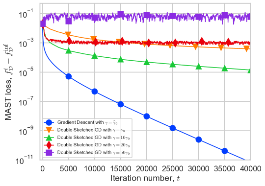
Figure 3: MAST loss (2) convergence with varying step size in case of Rand-$1$ sketches. We denote theoretical stepsizes as $\widehat{\gamma}_{0}=\frac{1}{L_{f}L_{\mathcal{D}}}$ and $\gamma_{0}=\frac{1}{L_{f}L^{\max}_{{\bf S}}}.$ Gradient Descent applied to MAST problem requires computing double sketched gradient for all possible ($N=d$) sketches.

In our final experiment depicted in Figure 3, we validate the claims of Theorem 2. We consider the same Logistic regression optimization problem (21) with $\lambda$ set to make sure $\kappa_{f}=10^{3}$. We use the whole dataset a1a and initialization $x^{0}=0$. Consider $\mathcal{D}$ as a uniform distribution over Rand-$K$ sketches for $K=1$. Then MAST stochastic optimization formulation (2) leads to a finite-sum problem over sketches ${\bf C}_{i}$, as defined in (17). This allows us to evaluate the performance of Algorithm 1 (I), which converges linearly for the exact MAST loss (2). Our findings accentuate the pivotal role of the appropriate step size $\gamma$ in steering the trajectory of sparse training. Guided by our theoretical framework, this step size must be adjusted in proportion to $K^{2}/d^{2}$ for Rand-$K$. Notably, for this particular problem at hand, a larger $\gamma$ (e.g., $\gamma=10\gamma_{0}$) can accelerate convergence. Yet, surpassing a delineated boundary can result in the stagnation of progress (e.g., $\gamma=20\gamma_{0}$) and, in specific scenarios, even derail the convergence altogether (e.g., $\gamma=50\gamma_{0}$). Such observations underscore the imperative of modulating the learning rate, especially within the realms of sparse and Dropout training.

References

- Alam et al. (2022) S. Alam, L. Liu, M. Yan, and M. Zhang. FedRolex: Model-heterogeneous federated learning with rolling sub-model extraction. In A. H. Oh, A. Agarwal, D. Belgrave, and K. Cho, editors, Advances in Neural Information Processing Systems, 2022. URL https://openreview.net/forum?id=OtxyysUdBE.
- Alistarh et al. (2018) D. Alistarh, T. Hoefler, M. Johansson, S. Khirirat, N. Konstantinov, and C. Renggli. The convergence of sparsified gradient methods. In Advances in Neural Information Processing Systems (NeurIPS), 2018.
- Allen (1971) D. M. Allen. Mean square error of prediction as a criterion for selecting variables. Technometrics, 13(3):469–475, 1971.
- Bertsekas (1977) D. P. Bertsekas. Approximation procedures based on the method of multipliers. Journal of Optimization Theory and Applications, 23(4):487–510, 1977.
- Bottou et al. (2018) L. Bottou, F. E. Curtis, and J. Nocedal. Optimization methods for large-scale machine learning. SIAM review, 60(2):223–311, 2018.
- Bouacida et al. (2021) N. Bouacida, J. Hou, H. Zang, and X. Liu. Adaptive federated dropout: Improving communication efficiency and generalization for federated learning. In IEEE INFOCOM 2021 - IEEE Conference on Computer Communications Workshops (INFOCOM WKSHPS), pages 1–6, 2021.
- Caldas et al. (2018) S. Caldas, J. Konečný, H. B. McMahan, and A. Talwalkar. Expanding the reach of federated learning by reducing client resource requirements. arXiv preprint arXiv:1812.07210, 2018.
- Chang and Lin (2011) C.-C. Chang and C.-J. Lin. LIBSVM: a library for support vector machines. ACM Transactions on Intelligent Systems and Technology (TIST), 2(3):1–27, 2011.
- Chang et al. (2021) X. Chang, Y. Li, S. Oymak, and C. Thrampoulidis. Provable benefits of overparameterization in model compression: From double descent to pruning neural networks. In Proceedings of the AAAI Conference on Artificial Intelligence, volume 35, pages 6974–6983, 2021.
- Charles et al. (2022) Z. Charles, K. Bonawitz, S. Chiknavaryan, B. McMahan, et al. Federated select: A primitive for communication-and memory-efficient federated learning. arXiv preprint arXiv:2208.09432, 2022.
- Chen et al. (2022) Y. Chen, Z. Chen, P. Wu, and H. Yu. FedOBD: Opportunistic block dropout for efficiently training large-scale neural networks through federated learning. arXiv preprint arXiv:2208.05174, 2022.
- Chraibi et al. (2019) S. Chraibi, A. Khaled, D. Kovalev, P. Richtárik, A. Salim, and M. Takáč. Distributed fixed point methods with compressed iterates. arXiv preprint arXiv:2102.07245, 2019.
- Condat et al. (2023) L. Condat, D. Kitahara, A. Contreras, and A. Hirabayashi. Proximal splitting algorithms for convex optimization: A tour of recent advances, with new twists. SIAM Review, 65(2):375–435, 2023.
- Demidovich et al. (2023) Y. Demidovich, G. Malinovsky, I. Sokolov, and P. Richtárik. A guide through the Zoo of biased SGD. arXiv preprint arXiv:2305.16296, 2023.
- Diao et al. (2021) E. Diao, J. Ding, and V. Tarokh. HeteroFL: Computation and communication efficient federated learning for heterogeneous clients. In International Conference on Learning Representations, 2021. URL https://openreview.net/forum?id=TNkPBBYFkXg.
- Drori and Shamir (2020) Y. Drori and O. Shamir. The complexity of finding stationary points with stochastic gradient descent. In International Conference on Machine Learning, pages 2658–2667. PMLR, 2020.
- Dun et al. (2022) C. Dun, C. R. Wolfe, C. M. Jermaine, and A. Kyrillidis. ResIST: Layer-wise decomposition of resnets for distributed training. In Uncertainty in Artificial Intelligence, pages 610–620. PMLR, 2022.
- Dun et al. (2023) C. Dun, M. Hipolito, C. Jermaine, D. Dimitriadis, and A. Kyrillidis. Efficient and light-weight federated learning via asynchronous distributed dropout. In International Conference on Artificial Intelligence and Statistics, pages 6630–6660. PMLR, 2023.
- Ermoliev (1988) Y. Ermoliev. Stochastic quasigradient methods. numerical techniques for stochastic optimization. Springer Series in Computational Mathematics, (10):141–185, 1988.
- Evci et al. (2019) U. Evci, F. Pedregosa, A. Gomez, and E. Elsen. The difficulty of training sparse neural networks. arXiv preprint arXiv:1906.10732, 2019.
- Evci et al. (2020) U. Evci, T. Gale, J. Menick, P. S. Castro, and E. Elsen. Rigging the lottery: Making all tickets winners. In International Conference on Machine Learning, pages 2943–2952. PMLR, 2020.
- Fan et al. (2019) A. Fan, E. Grave, and A. Joulin. Reducing transformer depth on demand with structured dropout. In International Conference on Learning Representations, 2019.
- Finn et al. (2017) C. Finn, P. Abbeel, and S. Levine. Model-agnostic meta-learning for fast adaptation of deep networks. In International Conference on Machine Learning, pages 1126–1135. PMLR, 2017.
- Frankle and Carbin (2018) J. Frankle and M. Carbin. The lottery ticket hypothesis: Finding sparse, trainable neural networks. In International Conference on Learning Representations, 2018.
- Frazier-Logue and Hanson (2018) N. Frazier-Logue and S. J. Hanson. Dropout is a special case of the stochastic delta rule: Faster and more accurate deep learning. arXiv preprint arXiv:1808.03578, 2018.
- Ghadimi and Lan (2013) S. Ghadimi and G. Lan. Stochastic first-and zeroth-order methods for nonconvex stochastic programming. SIAM Journal on Optimization, 23(4):2341–2368, 2013.
- Gomez et al. (2019) A. N. Gomez, I. Zhang, S. R. Kamalakara, D. Madaan, K. Swersky, Y. Gal, and G. E. Hinton. Learning sparse networks using targeted dropout. arXiv preprint arXiv:1905.13678, 2019.
- Goodfellow et al. (2016) I. Goodfellow, Y. Bengio, and A. Courville. Deep learning. MIT press, 2016.
- Gorbunov et al. (2020) E. Gorbunov, F. Hanzely, and P. Richtárik. A unified theory of SGD: Variance reduction, sampling, quantization and coordinate descent. In International Conference on Artificial Intelligence and Statistics, pages 680–690. PMLR, 2020.
- Gower et al. (2019) R. M. Gower, N. Loizou, X. Qian, A. Sailanbayev, E. Shulgin, and P. Richtárik. SGD: General analysis and improved rates. Proceedings of the 36th International Conference on Machine Learning, Long Beach, California, 2019.
- Gower et al. (2020) R. M. Gower, M. Schmidt, F. Bach, and P. Richtárik. Variance-reduced methods for machine learning. Proceedings of the IEEE, 108(11):1968–1983, 2020.
- Guo et al. (2016) Y. Guo, A. Yao, and Y. Chen. Dynamic network surgery for efficient dnns. Advances in Neural Information Processing Systems, 29, 2016.
- Hanson (1990) S. J. Hanson. A stochastic version of the delta rule. Physica D: Nonlinear Phenomena, 42(1-3):265–272, 1990.
- Hanzely and Richtárik (2020) F. Hanzely and P. Richtárik. Federated learning of a mixture of global and local models. arXiv preprint arXiv:2002.05516, 2020.
- Hearst et al. (1998) M. A. Hearst, S. T. Dumais, E. Osuna, J. Platt, and B. Scholkopf. Support vector machines. IEEE Intelligent Systems and their applications, 13(4):18–28, 1998.
- Hinton et al. (2012) G. E. Hinton, N. Srivastava, A. Krizhevsky, I. Sutskever, and R. R. Salakhutdinov. Improving neural networks by preventing co-adaptation of feature detectors. arXiv preprint arXiv:1207.0580, 2012.
- Hoefler et al. (2021) T. Hoefler, D. Alistarh, T. Ben-Nun, N. Dryden, and A. Peste. Sparsity in deep learning: Pruning and growth for efficient inference and training in neural networks. The Journal of Machine Learning Research, 22(1):10882–11005, 2021.
- Hofmann et al. (2015) T. Hofmann, A. Lucchi, S. Lacoste-Julien, and B. McWilliams. Variance reduced stochastic gradient descent with neighbors. Advances in Neural Information Processing Systems, 28, 2015.
- Holland and Welsch (1977) P. W. Holland and R. E. Welsch. Robust regression using iteratively reweighted least-squares. Communications in Statistics-theory and Methods, 6(9):813–827, 1977.
- Horváth et al. (2021) S. Horváth, S. Laskaridis, M. Almeida, I. Leontiadis, S. Venieris, and N. Lane. FjORD: Fair and accurate federated learning under heterogeneous targets with ordered dropout. Advances in Neural Information Processing Systems, 34:12876–12889, 2021.
- J Reddi et al. (2015) S. J Reddi, A. Hefny, S. Sra, B. Poczos, and A. J. Smola. On variance reduction in stochastic gradient descent and its asynchronous variants. Advances in neural information processing systems, 28, 2015.
- Jiang et al. (2022) Y. Jiang, S. Wang, V. Valls, B. J. Ko, W.-H. Lee, K. K. Leung, and L. Tassiulas. Model pruning enables efficient federated learning on edge devices. IEEE Transactions on Neural Networks and Learning Systems, 2022.
- Kairouz et al. (2021) P. Kairouz, H. B. McMahan, B. Avent, A. Bellet, M. Bennis, A. N. Bhagoji, K. A. Bonawitz, Z. Charles, G. Cormode, R. Cummings, R. G. L. D’Oliveira, H. Eichner, S. E. Rouayheb, D. Evans, J. Gardner, Z. Garrett, A. Gascón, B. Ghazi, P. B. Gibbons, M. Gruteser, Z. Harchaoui, C. He, L. He, Z. Huo, B. Hutchinson, J. Hsu, M. Jaggi, T. Javidi, G. Joshi, M. Khodak, J. Konečný, A. Korolova, F. Koushanfar, S. Koyejo, T. Lepoint, Y. Liu, P. Mittal, M. Mohri, R. Nock, A. Özgür, R. Pagh, H. Qi, D. Ramage, R. Raskar, M. Raykova, D. Song, W. Song, S. U. Stich, Z. Sun, A. T. Suresh, F. Tramèr, P. Vepakomma, J. Wang, L. Xiong, Z. Xu, Q. Yang, F. X. Yu, H. Yu, and S. Zhao. Advances and open problems in federated learning. Found. Trends Mach. Learn., 14(1-2):1–210, 2021. doi: 10.1561/2200000083. URL https://doi.org/10.1561/2200000083.
- Khaled and Richtárik (2019) A. Khaled and P. Richtárik. Gradient descent with compressed iterates. NeurIPS 2019 Workshop on Federated Learning for Data Privacy and Confidentiality, 2019.
- Khaled and Richtárik (2023) A. Khaled and P. Richtárik. Better theory for SGD in the nonconvex world. Transactions on Machine Learning Research, 2023. ISSN 2835-8856. URL https://openreview.net/forum?id=AU4qHN2VkS. Survey Certification.
- Khaled et al. (2020) A. Khaled, K. Mishchenko, and P. Richtárik. Tighter theory for local SGD on identical and heterogeneous data. In International Conference on Artificial Intelligence and Statistics, pages 4519–4529. PMLR, 2020.
- Khaled et al. (2023) A. Khaled, O. Sebbouh, N. Loizou, R. M. Gower, and P. Richtárik. Unified analysis of stochastic gradient methods for composite convex and smooth optimization. Journal of Optimization Theory and Applications, pages 1–42, 2023.
- Khirirat et al. (2018) S. Khirirat, H. R. Feyzmahdavian, and M. Johansson. Distributed learning with compressed gradients. arXiv preprint arXiv:1806.06573, 2018.
- Konečný et al. (2016) J. Konečný, H. B. McMahan, F. X. Yu, P. Richtárik, A. T. Suresh, and D. Bacon. Federated learning: Strategies for improving communication efficiency. NIPS Private Multi-Party Machine Learning Workshop, 2016.
- Kovalev et al. (2020) D. Kovalev, S. Horváth, and P. Richtárik. Don’t jump through hoops and remove those loops: SVRG and Katyusha are better without the outer loop. In Algorithmic Learning Theory, pages 451–467. PMLR, 2020.
- Li et al. (2020) Z. Li, H. Bao, X. Zhang, and P. Richtarik. PAGE: A simple and optimal probabilistic gradient estimator for nonconvex optimization. arXiv preprint arXiv:2008.10898, 2020.
- Liao and Kyrillidis (2022) F. Liao and A. Kyrillidis. On the convergence of shallow neural network training with randomly masked neurons. Transactions on Machine Learning Research, 2022. URL https://openreview.net/forum?id=e7mYYMSyZH.
- Lin et al. (2019) T. Lin, S. U. Stich, L. Barba, D. Dmitriev, and M. Jaggi. Dynamic model pruning with feedback. In International Conference on Learning Representations, 2019.
- Louizos et al. (2018) C. Louizos, M. Welling, and D. P. Kingma. Learning sparse neural networks through l_0 regularization. In International Conference on Learning Representations, 2018.
- Mansour et al. (2020) Y. Mansour, M. Mohri, J. Ro, and A. T. Suresh. Three approaches for personalization with applications to federated learning. arXiv preprint arXiv:2002.10619, 2020.
- McMahan et al. (2017) B. McMahan, E. Moore, D. Ramage, S. Hampson, and B. A. y Arcas. Communication-efficient learning of deep networks from decentralized data. In Artificial Intelligence and Statistics, pages 1273–1282. PMLR, 2017.
- Mianjy and Arora (2020) P. Mianjy and R. Arora. On convergence and generalization of dropout training. Advances in Neural Information Processing Systems, 33:21151–21161, 2020.
- Mishchenko et al. (2020) K. Mishchenko, A. Khaled, and P. Richtárik. Random reshuffling: Simple analysis with vast improvements. Advances in Neural Information Processing Systems, 33:17309–17320, 2020.
- Mocanu et al. (2016) D. C. Mocanu, E. Mocanu, P. H. Nguyen, M. Gibescu, and A. Liotta. A topological insight into restricted boltzmann machines. Machine Learning, 104:243–270, 2016.
- Mocanu et al. (2018) D. C. Mocanu, E. Mocanu, P. Stone, P. H. Nguyen, M. Gibescu, and A. Liotta. Scalable training of artificial neural networks with adaptive sparse connectivity inspired by network science. Nature Communications, 9(1):2383, 2018.
- Mohtashami et al. (2022) A. Mohtashami, M. Jaggi, and S. Stich. Masked training of neural networks with partial gradients. In International Conference on Artificial Intelligence and Statistics, pages 5876–5890. PMLR, 2022.
- Moulines and Bach (2011) E. Moulines and F. Bach. Non-asymptotic analysis of stochastic approximation algorithms for machine learning. In J. Shawe-Taylor, R. Zemel, P. Bartlett, F. Pereira, and K. Weinberger, editors, Advances in Neural Information Processing Systems, volume 24. Curran Associates, Inc., 2011. URL https://proceedings.neurips.cc/paper_files/paper/2011/file/40008b9a5380fcacce3976bf7c08af5b-Paper.pdf.
- Nesterov (1983) Y. Nesterov. A method of solving a convex programming problem with convergence rate . Doklady Akademii Nauk USSR, 269(3):543–547, 1983.
- Nikdan et al. (2023) M. Nikdan, T. Pegolotti, E. Iofinova, E. Kurtic, and D. Alistarh. SparseProp: Efficient sparse backpropagation for faster training of neural networks at the edge. In A. Krause, E. Brunskill, K. Cho, B. Engelhardt, S. Sabato, and J. Scarlett, editors, Proceedings of the 40th International Conference on Machine Learning, volume 202 of Proceedings of Machine Learning Research, pages 26215–26227. PMLR, 23–29 Jul 2023. URL https://proceedings.mlr.press/v202/nikdan23a.html.
- Peste et al. (2021) A. Peste, E. Iofinova, A. Vladu, and D. Alistarh. AC/DC: Alternating compressed/decompressed training of deep neural networks. Advances in neural information processing systems, 34:8557–8570, 2021.
- Poljak (1979) B. Poljak. On the bertsekas’ method for minimization of composite functions. In International Symposium on Systems Optimization and Analysis, pages 178–186. Springer Berlin/Heidelberg, 1979.
- Qiu et al. (2022) X. Qiu, J. Fernandez-Marques, P. P. Gusmao, Y. Gao, T. Parcollet, and N. D. Lane. ZeroFL: Efficient on-device training for federated learning with local sparsity. In International Conference on Learning Representations, 2022. URL https://openreview.net/forum?id=2sDQwC_hmnM.
- Richtárik et al. (2021) P. Richtárik, I. Sokolov, and I. Fatkhullin. Ef21: A new, simpler, theoretically better, and practically faster error feedback. arXiv preprint arXiv:2106.05203, 2021.
- Robbins and Monro (1951) H. Robbins and S. Monro. A stochastic approximation method. The Annals of Mathematical Statistics, pages 400–407, 1951.
- Schmidhuber (1987) J. Schmidhuber. Evolutionary principles in self-referential learning, or on learning how to learn: the meta-meta-… hook. PhD thesis, Technische Universität München, 1987.
- Seide et al. (2014) F. Seide, H. Fu, J. Droppo, G. Li, and D. Yu. 1-bit stochastic gradient descent and its application to data-parallel distributed training of speech DNNs. In Fifteenth Annual Conference of the International Speech Communication Association, 2014.
- Senen-Cerda and Sanders (2020) A. Senen-Cerda and J. Sanders. Almost sure convergence of dropout algorithms for neural networks. arXiv preprint arXiv:2002.02247, 2020.
- Senen-Cerda and Sanders (2022) A. Senen-Cerda and J. Sanders. Asymptotic convergence rate of dropout on shallow linear neural networks. Proceedings of the ACM on Measurement and Analysis of Computing Systems, 6(2):1–53, 2022.
- Shulgin and Richtárik (2022) E. Shulgin and P. Richtárik. Shifted compression framework: Generalizations and improvements. In The 38th Conference on Uncertainty in Artificial Intelligence, 2022.
- Shulgin and Richtárik (2023) E. Shulgin and P. Richtárik. Towards a better theoretical understanding of independent subnetwork training. arXiv preprint arXiv:2306.16484, 2023.
- Smith et al. (2017) V. Smith, C.-K. Chiang, M. Sanjabi, and A. S. Talwalkar. Federated multi-task learning. Advances in neural information processing systems, 30, 2017.
- Srivastava et al. (2014) N. Srivastava, G. Hinton, A. Krizhevsky, I. Sutskever, and R. Salakhutdinov. Dropout: a simple way to prevent neural networks from overfitting. The journal of machine learning research, 15(1):1929–1958, 2014.
- Stich and Karimireddy (2020) S. U. Stich and S. P. Karimireddy. The error-feedback framework: SGD with delayed gradients. Journal of Machine Learning Research, 21(237):1–36, 2020. URL http://jmlr.org/papers/v21/19-748.html.
- Stich et al. (2018) S. U. Stich, J.-B. Cordonnier, and M. Jaggi. Sparsified SGD with memory. In Advances in Neural Information Processing Systems, pages 4447–4458, 2018.
- Sun (2020) R.-Y. Sun. Optimization for deep learning: An overview. Journal of the Operations Research Society of China, 8(2):249–294, 2020.
- Szlendak et al. (2022) R. Szlendak, A. Tyurin, and P. Richtárik. Permutation compressors for provably faster distributed nonconvex optimization. In International Conference on Learning Representations, 2022. URL https://openreview.net/forum?id=GugZ5DzzAu.
- Szlendak et al. (2023) R. Szlendak, E. Gasanov, and P. Richtárik. Understanding progressive training through the framework of randomized coordinate descent. arXiv preprint arXiv:2306.03626, 2023.
- Villalobos et al. (2022) P. Villalobos, J. Sevilla, T. Besiroglu, L. Heim, A. Ho, and M. Hobbhahn. Machine learning model sizes and the parameter gap. arXiv preprint arXiv:2207.02852, 2022.
- Wan et al. (2013) L. Wan, M. Zeiler, S. Zhang, Y. Le Cun, and R. Fergus. Regularization of neural networks using dropconnect. In International Conference on Machine Learning, pages 1058–1066. PMLR, 2013.
- Wang et al. (2022) H.-P. Wang, S. Stich, Y. He, and M. Fritz. Progfed: effective, communication, and computation efficient federated learning by progressive training. In International Conference on Machine Learning, pages 23034–23054. PMLR, 2022.
- Wang and Manning (2013) S. Wang and C. Manning. Fast dropout training. In International Conference on Machine Learning, pages 118–126. PMLR, 2013.
- Wang et al. (2018) S. Wang, T. Tuor, T. Salonidis, K. K. Leung, C. Makaya, T. He, and K. Chan. When edge meets learning: Adaptive control for resource-constrained distributed machine learning. In IEEE INFOCOM 2018-IEEE Conference on Computer Communications, pages 63–71. IEEE, 2018.
- Wangni et al. (2018) J. Wangni, J. Wang, J. Liu, and T. Zhang. Gradient sparsification for communication-efficient distributed optimization. In Advances in Neural Information Processing Systems, pages 1299–1309, 2018.
- Waskom (2021) M. L. Waskom. seaborn: statistical data visualization. Journal of Open Source Software, 6(60):3021, 2021. doi: 10.21105/joss.03021. URL https://doi.org/10.21105/joss.03021.
- Wen et al. (2022) D. Wen, K.-J. Jeon, and K. Huang. Federated dropout—a simple approach for enabling federated learning on resource constrained devices. IEEE Wireless Communications Letters, 11(5):923–927, 2022.
- Wolfe et al. (2023) C. R. Wolfe, J. Yang, F. Liao, A. Chowdhury, C. Dun, A. Bayer, S. Segarra, and A. Kyrillidis. GIST: Distributed training for large-scale graph convolutional networks. Journal of Applied and Computational Topology, pages 1–53, 2023.
- Wu et al. (2016) J. Wu, C. Leng, Y. Wang, Q. Hu, and J. Cheng. Quantized convolutional neural networks for mobile devices. In Proceedings of the IEEE Conference on Computer Vision and Pattern Recognition, pages 4820–4828, 2016.
- Yang et al. (2017) T.-J. Yang, Y.-H. Chen, J. Emer, and V. Sze. A method to estimate the energy consumption of deep neural networks. In 2017 51st Asilomar Conference on Signals, Systems, and Computers, pages 1916–1920. IEEE, 2017.
- Yang et al. (2022) T.-J. Yang, D. Guliani, F. Beaufays, and G. Motta. Partial variable training for efficient on-device federated learning. In ICASSP 2022-2022 IEEE International Conference on Acoustics, Speech and Signal Processing (ICASSP), pages 4348–4352. IEEE, 2022.
- Yuan et al. (2022) B. Yuan, C. R. Wolfe, C. Dun, Y. Tang, A. Kyrillidis, and C. Jermaine. Distributed learning of fully connected neural networks using independent subnet training. Proceedings of the VLDB Endowment, 15(8):1581–1590, 2022.
- Zhang and Sabuncu (2018) Z. Zhang and M. Sabuncu. Generalized cross entropy loss for training deep neural networks with noisy labels. Advances in Neural Information Processing Systems, 31, 2018.
- Zhou et al. (2022) H. Zhou, T. Lan, G. Venkataramani, and W. Ding. On the convergence of heterogeneous federated learning with arbitrary adaptive online model pruning. arXiv preprint arXiv:2201.11803, 2022. URL https://openreview.net/forum?id=p3EhUXVMeyn.