Paramagnetic contribution in superconductors with different-mass Cooper pairs

Abstract

Cooper pairs formed by two electrons with different effective mass are common in multiband superconductors, pair density wave states and other superconducting systems with multi-degrees of freedom. In this work, we show that there are paramagnetic contributions to the superfluid stiffness in superconductors with different-mass Cooper pairs. This paramagnetic response is owing to the relative motion between two electrons with different mass. We investigate the paramagnetic contributions based on the linear response theory in two-band superconductors with interband pairings and in pair density wave states respectively. Our results offer a new perspective to the electromagnetic superfluid stiffness in unconventional superconductors beyond BCS theory.

Superconductors (SCs) are defined by zero resistance and Meissner effect with perfect diamagnetism Schrieffer (1964). Microscopically, the central ingredients for superconductors are the Cooper pairs and their phase coherence, in which electrons bind together two by two and condense to form a coherent quantum state Schrieffer (1964); Bardeen et al. (1957). Especially, the phase coherence plays an essential role in the electromagnetic response of SCs. Any phase disturbance induced by external magnetic fields is disfavored by Cooper pairs’ phase coherence leading to the diamagnetic Meissner effect. The diamagnetic rigidity in SCs are normally characterized by the superfliud stiffness $\rho_{s}$, which is defined in the London equation coefficient as $\mathbf{j}=-\frac{4e^{2}}{\hbar^{2}}\rho_{s}\mathbf{A}=\frac{1}{\lambda^{2}}\mathbf{A}$ Schrieffer (1964); Coleman (2015); Scalapino et al. (1993). As schematically illustrated in Fig.1(a), Cooper pairs’ diamagnetic supercurrent expels the magnetic field from the interior of the superconductor with a characteristic penetration depth $\lambda$. Understanding superfliud stiffness is not only one key question in BCS theory Schrieffer (1964); Bardeen et al. (1957), but also a window towards understanding high-temperature superconductors Xiang and Wu (2022); Uemura et al. (1993); Božović et al. (2016, 2018); Mahmood et al. (2019); Lee-Hone et al. (2020); Wang et al. (2022); Li et al. (2021).

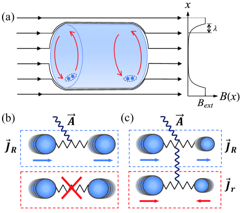
Figure 1: (a) Schematic diagram of the Meissner effect for superconductors. The red arrow indicates the Cooper pairs’ supercurrent, which expels the magnetic field from the interior of the superconductor, as shown in the right panel. (b,c) Schematic diagram of the response current to the electromagnetic field of the two-electron pair with (b) equal mass, (c) different mass. In case (b), there is no $\bf{J}_{r}$ contribution and gauge field $\mathbf{A}$ couples with $\bf{J}_{R}$. In case (c), the $\bf{J}_{r}$ contributes owing to its coupling with $\bf{J}_{R}$. $\bf{J}_{r}$ plays the key role in paramagnetic response.

On the other hand, Cooper pairs are formed by two electrons. Since effective mass of electrons can vary dramatically in a solid state system, there are superconducting pairing systems with Cooper pairs formed by two electrons with different effective mass, namely the different-mass Copper pair systems. The different-mass Copper pair systems are common in superconductors. For example, in multiband systems, interband pairings between two different electron bands generically provide different-mass Copper pairsSuhl et al. (1959); a pair density wave state (PDW) with vector $Q$ connecting $k$ and $-k+Q$ sectors can easily host different mass Cooper pairs as wellAgterberg et al. (2020a). Therefore, it is natural to ask whether new properties can be associated to the different-mass pairing. In this work, we show that different mass Cooper pairs, surprisingly, carry out a new paramagnetic response. The paramagnetic contribution is important to understand the superfluid stiffness in unconventional superconducting states.

To investigate the electromagnetic response of SC with different-mass Cooper pairs, we start from how a system with two different-mass electrons couples to the electromagnetic gauge field ${\bf A}$ from a Cooper problem Cooper (1956). The kinetic part Hamiltonian of this Cooper problem can be written as

$$H_{c}=\frac{\left[-{\mathrm{i}}\bf{\nabla}_{{\bf r}_{1}}-e{\bf A}({\bf r}_{1})\right]^{2}}{2m_{1}}+\frac{\left[-{\mathrm{i}}\bf{\nabla}_{{\bf r}_{2}}-e{\bf A}({\bf r}_{2})\right]^{2}}{2m_{2}}$$ (1)

Using the center-of-mass (COM) coordinate ${\bf R}=\frac{{\bf r}_{1}+{\bf r}_{2}}{2}$, the relative coordinate $\bar{{\bf r}}={\bf r}_{1}-{\bf r}_{2}$ and their corresponding mass $M_{\pm}^{-1}=m_{1}^{-1}\pm m_{2}^{-1}$, the Hamiltonian $H_{c}$ transforms into

$$H_{c} = \frac{1}{2M_{+}}\left[-{\mathrm{i}}\frac{\nabla_{{\bf R}}}{2}-e{\bf A}({\bf R})\right]^{2}+\frac{\left(-{\mathrm{i}}\nabla_{\bar{{\bf r}}}\right)^{2}}{2M_{-}}+$$ (2)

$$\qquad\qquad\frac{1}{2M_{-}}\left\{-{\mathrm{i}}\frac{\nabla_{{\bf R}}}{2}-e{\bf A}({\bf R}),-{\mathrm{i}}\nabla_{\bar{{\bf r}}}\right\}.$$

From Eq. 2, we can see the first term describing the energy of COM coupled to the gauge field $\mathbf{A}$, which contains both the paramagnetic and diamagnetic contribution. Note that we approximate the vector potential as ${\bf A}({\bf R}\pm\bar{{\bf r}}/2)\approx{\bf A}({\bf R})$, due to the slowly varying field. The second term $\left(-{\mathrm{i}}\nabla_{\bar{{\bf r}}}\right)^{2}/2M_{-}$ describes the kinetic energy of the relative motion without coupling to the gauge field because the relative motion is a charge-less process. The last term $\frac{1}{2M_{-}}\left\{-{\mathrm{i}}\frac{\nabla_{{\bf R}}}{2}-e{\bf A}({\bf R}),-{\mathrm{i}}\nabla_{\bar{{\bf r}}}\right\}$ describes the coupling between the COM motion and relative motion, which plays an important role in linking the relative motion to the gauge field as discussed later.

Taking the $H_{c}$ derivative respective to $\mathbf{A}$, the response current $\bf{J}$ is obtained with two contribution from COM and relative motions as $\mathbf{J}=-\partial H_{c}/\partial{\bf A}=\bf{J}_{R}+\bf{J}_{r}$, as schematically plotted in Fig.1(b,c). Starting from the equal mass limit with $M_{-}=0$, the last two terms in $H_{c}$ vanishes. Hence, there only remains the current $\bf{J}_{R}$ from COM motion, as shown in Fig.1(b). On the other hand, for the Cooper pair with different mass plotted in Fig.1(c), both $\bf{J}_{R}$ in the up panel and $\bf{J}_{r}$ in the lower panel exist. Especially, the $\bf{J}_{r}$ emerges from the coupling between COM motion and relative motion in the last term of $H_{c}$.

In other words, if the two different-mass electrons form the Cooper pair in SC, the COM part performs like the Cooper pair composed of the equal mass electrons. The electromagnetic response of COM shows perfect diamagnetism, where the paramagnetic response is strictly zero. However, the relative motion contributes a paramagnetic response, resulting in the reduction of the superfluid stiffness owing to the vanishing diamagnetic term related to $M_{-}$ in $\left(-{\mathrm{i}}\nabla_{\bar{{\bf r}}}\right)^{2}/2M_{-}$.

To illustrate above ideas, we first study the superfluid stiffness in the multiband SCs with interband pairing. The multiband effect in superconductivity is a long-term topic Suhl et al. (1959), since the discovery of BCS theory. The multiple band signatures have been widely observed in superconductors, including elemental metals Nb, Ta, V and Pb Shen et al. (1965); Blackford and March (1969), MgB₂ Souma et al. (2003), doped-SrTiO₃ Schooley et al. (1964), especially the iron pnictides and chalcogenides Kamihara et al. (2008); Takahashi et al. (2008); Paglione and Greene (2010). Here, we consider a simplified two-band model with interband pairing:

$$H_{\mathbf{k}}=\sum_{\alpha,\sigma}\xi_{\alpha}(\mathbf{k})c_{\mathbf{k},\alpha,\sigma}^{\dagger}c_{\mathbf{k},\alpha,\sigma}+\Delta\sum_{\alpha\neq\beta}\left(c_{\mathbf{k},\alpha,\uparrow}^{\dagger}c_{-\mathbf{k},\beta,\downarrow}^{\dagger}+\text{ H.c. }\right)$$ (3)

where $\alpha,\beta=1,2$ label two separated bands. These two bands host the dispersion $\xi_{\alpha}(k)=\frac{k^{2}}{2m_{\alpha}}-\mu$ with mass $m_{\alpha}$ and chemical potential $\mu$, as the red and blue parabolic bands illustrated in Fig.2(a). $\Delta$ is the mean-field interband pairing order parameter. Normally, this interband pairing should not be the leading pairing instability. However, we take a phenomenology approach to this problem and assume the interband pairing is dominated in this toy model. Below we define $\gamma_{\alpha}=\frac{1}{2m_{\alpha}}$ for convenience. Under the basis $\Psi_{k}^{\dagger}=\{c_{1k\uparrow}^{\dagger},c_{2k\uparrow}^{\dagger},c_{1,-k\downarrow},c_{2,-k\downarrow}\}^{\mathrm{T}}$, the BdG Hamiltonian can be written as

$$H_{BdG}=\left(\begin{array}[]{cccc}\gamma_{1}k^{2}-\mu&0&0&\Delta\\ 0&\gamma_{2}k^{2}-\mu&\Delta&0\\ 0&\Delta&-\gamma_{1}k^{2}+\mu&0\\ \Delta&0&0&-\gamma_{2}k^{2}+\mu\end{array}\right).$$ (4)

where $k^{2}=k_{x}^{2}+k_{y}^{2}$. The Hamiltonian is composed of two decoupled blocks, which are particle-hole related. Thus, we can focus on the $H_{1}$ block for convenience as

$$H_{1}=\left(\begin{array}[]{cc}\gamma_{1}k^{2}-\mu&\Delta\\ \Delta&-\gamma_{2}k^{2}+\mu\end{array}\right).$$ (5)

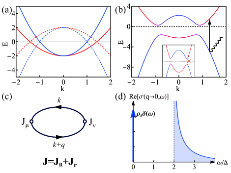
Figure 2: (a) The energy of the two parabolic bands with different mass. The dashed line is the particle-hole symmetric band. (b) The band structure of the two different-mass band superconductor with inter-band pairing. The arrow represents the direct transition between the two asymmetric Bogoliubov band due to the optical absorption. Inset: the case of the two bands with the equal mass where the optical process is forbidden. (c) The Feynman diagram of the current-current correlation. (d) The complex optical conductance spectrum of the system. The zero frequency peak $\rho_{s}\delta(\omega)$ is from superfluid while the area under $\sigma(\omega\neq 0)$ is proportional to paramagnetic contribution $\Pi_{\mu\nu}$. The parameters used in the calculation are $\gamma_{1}=1$, $\gamma_{2}=2$, $\mu=2$ and $\Delta=1$.

The eigenvalue of $H_{1}$ are $E_{k}^{\pm}=\eta_{k}\pm\sqrt{\epsilon_{k}^{2}+\Delta^{2}}$, where $\eta_{k}=\frac{\gamma_{1}-\gamma_{2}}{2}k^{2}$ and $\epsilon_{k}=\frac{\gamma_{1}+\gamma_{2}}{2}k^{2}-\mu$. Note that the system is fully gapped only when $\Delta>\frac{\mu\absolutevalue{\gamma_{1}-\gamma_{2}}}{2\sqrt{\gamma_{1}\gamma_{2}}}$, namely $E_{k}^{+}>0$ and $E_{k}^{-}<0$. Fig.2(b) shows the band dispersion of $H_{1}$ block in the fully-gapped region. The color of the band represents the weight of the two band in Fig.2(a). It’s obvious that the two band is not particle-hole symmetric because of the $\eta_{k}$ contribution in this block. This $\eta_{k}$ is just the contribution from the relative motion. The particle-hole symmetry is recovered for all bands in $H_{BdG}$.

The next step is to find the superfluid stiffness. Within linear response theory, the response current to the vector potential of electromagnetic field can be obtained via $J_{\mu}({{\bf q}},\Omega)=-\sum_{\nu}K_{\mu\nu}({{\bf q}},\Omega)A_{\nu}({{\bf q}},\Omega)$. Here $K_{\mu\nu}$ is the electromagnetic response tensor with two part of contributions, paramagnetic response from current-current correlation function $\Pi_{\mu\nu}$ and diamagnetic response from charge density $\langle\frac{\hat{n}}{m}\rangle$ as $K_{\mu\nu}=-e^{2}(\Pi_{\mu\nu}+\langle\frac{\hat{n}}{m}\rangle)$. According to London equation,the superfluid stiffness can be defined via $\rho_{s}=\frac{\hbar^{2}}{4e^{2}}\real K_{\mu\mu}(\omega=0,q\xrightarrow{}0)$. Notice that the paramagnetic current obtained from Eq.5 can be decomposed into two components as discussed above: the COM motion and the relative motion,

$$J^{P}(q) = J^{P}_{R}+J^{P}_{r}=\frac{\gamma_{1}+\gamma_{2}}{2}(2k+q)\sigma_{0}+\frac{\gamma_{1}-\gamma_{2}}{2}(2k+q)\sigma_{3}$$

Then the current-current correlation function can be calculated by $\Pi_{\mu\nu}(q,{\mathrm{i}}\Omega_{n})=\frac{1}{V\beta}\sum_{k,{\mathrm{i}}\omega_{n}}\Tr[J^{P}_{\mu}\mathcal{G}J^{P}_{\nu}\mathcal{G}]$ as the Feynman diagram in Fig.2(c), where $\mathcal{G}$ is the Green’s function for $H_{1}$ (see Supplemental Material (SM) for more details).

At zero temperature, considering the complete model given in Eq.4, the paramagnetic contribution of the superfluid response of this system with interband pairing is

$$\real\Pi_{\mu\nu}(\Omega=0,q\to 0)=-\frac{2(\gamma_{1}-\gamma_{2})^{2}\epsilon_{F}N_{\gamma^{+}}(0)}{\gamma_{1}+\gamma_{2}}\delta_{\mu\nu}$$ (6)

where $N_{\gamma^{+}}$ is the DOS of the 2D free electron gas with energy dispersion $\epsilon_{k}$, which is proportional to $\frac{1}{\gamma_{1}+\gamma_{2}}$. The factor $2$ comes from the equivalence when exchanging $\gamma_{1}$ and $\gamma_{2}$. This nonzero paramagnetic contribution is the key finding in this work. We can also calculate the diamagnetic contribution $\langle\frac{\hat{n}}{m}\rangle=2(\gamma_{1}+\gamma_{2})n_{c}$, where $n_{c}$ is the number of carriers in either band. (More details of the calculation can be found in SM.)

The paramagnetic contrition $\real\Pi_{\mu\nu}(\Omega=0,q\to 0)$ vanishes if $\gamma_{1}=\gamma_{2}$, which corresponds to the Cooper pairs composed of the equal mass electrons. This is consistent with the conventional BCS theory, where the $\Pi_{\mu\nu}$ contribution is strictly zero owing to the SC gap. Hence, the SC shows perfect diamagnetism from $\langle\frac{\hat{n}}{m}\rangle$ due to the vanishing $\Pi_{\mu\nu}$. On the other hand, if $\gamma_{1}\neq\gamma_{2}$, the paramagnetic response $\Pi_{\mu\nu}$ remains finite at zero temperature. Although the whole SC system remains diamagnetism, the existence of relative motion current $J^{P}_{r}(q)$ reduces the superfluid stiffness with finite $\Pi_{\mu\nu}$.

Actually the above results can be understood from the optical perspective. In the optical response, the optical conductivity $\sigma(\omega)$ follow a sum rule $\int_{0}^{\infty}\real\sigma(\omega)=\langle\frac{\pi e^{2}}{2m}\hat{n}\rangle$ Ferrell and Glover (1958); Tinkham and Ferrell (1959). For clean SCs in BCS theory, all the optical weight transfers into the $\omega=0$ with $\rho_{s}\delta(\omega)$ with $\real\sigma(\omega\neq 0)=0$. This $\real\sigma(\omega\neq 0)=0$ is due to the forbidden optical selection rule from particle-hole symmetry, as proved in Ref. Ahn and Nagaosa (2021) and illustrated in Fig.2(b) inset. However, this situation changes in the multiband system Ahn and Nagaosa (2021). The $\sigma(\omega\neq 0)$ becomes finite, as calculated in Fig.2(d). To satisfy optical sum rule, the superfluid stiffness in $\delta(\omega)$ must have finite $\Pi_{\mu\nu}$ contribution.

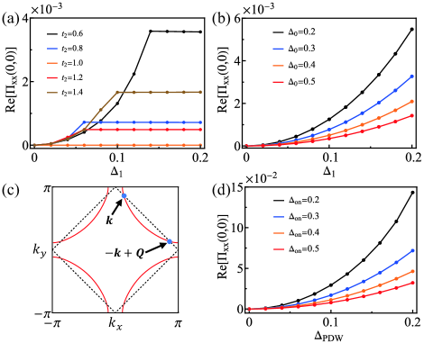
Figure 3: (a) The paramagnetic response of the two-band lattice model with only interband pairing for different hopping parameter. (b) The paramagnetic response of the two-band lattice model with both intraband and interband pairing. (c) The first Brillouin zone (BZ) of the square lattice. The red lines represent the Fermi surface (FS) of the dispersion in Eq.7. The arrows show the $k$ on the FS and its counterpart $-k+Q$ forming PDW Cooper pairs with $Q=(\pi,\pi)$. The dashed lines are the reduced BZ. (d) The paramagnetic response of the $(\pi,\pi)$-PDW with finite onsite pairing.

To further demonstrate above analytical results, we can numerically calculate the paramagnetic response using lattice models. Here we consider two band model on square lattice with the energy dispersion $\xi_{1,2}=-2t_{1,2}\left(\cos{k_{x}}+\cos{k_{y}}\right)-\mu$, where $t_{1,2}$ is the nearest-neighbor hopping parameter for band 1,2 respectively. We set $t_{1}=1$ as an energy scale. The ratio of the effective mass, defined by $m^{*}=\left(\frac{\partial^{2}\xi_{k}}{\partial k^{2}}\right)^{-1}$ of two energy bands is $m^{*}_{1}/m^{*}_{2}=t_{2}/t_{1}$. The paramagnetic responses $\real\Pi_{xx}(\Omega=0,q\to 0)$ as a function of interband pairing order parameter $\Delta_{1}$ for different value of $t_{2}$ are plotted in in Fig.3(a). Notice that, as we fix intraband pairing to zero, the system is gapless with Bogoliubov Fermi surface contributed by the lower quasiparticle band when $\Delta_{1}$ is small. Here we only focus on the interband transition process as shown by the arrow in Fig.2(b), although the Bogoliubov Fermi surface also contributes to the paramagnetic response through the intraband process.

From Fig.3(a), we can find that the paramagnetic response is always zero for any $\Delta_{1}$ at $t_{1}=t_{2}$, which corresponds to $m_{1}=m_{2}$. For $t_{1}\neq t_{2}$, the interband process starts to generate finite response. For small value of interband pairing, the $\Pi_{xx}$ response strengthens as $\Delta_{1}$ increases. This is because the only the quasiparticles under the Fermi surface contribute to the paramagnetic response, whose number increases as $\Delta_{1}$ increases. After $\Delta_{1}$ exceeds a critical value $\Delta_{c}$, the Bogoliubov Fermi surface disappears, and all quasiparticles in the lower band participate in interband processes, leading to a saturated response. We can also find that the saturated response is positively correlated with $\absolutevalue{t_{1}-t_{2}}$ and negatively correlated with $t_{1}+t_{2}$. These are consistent with the our analytical calculation results based on the effective continuum model.

In more realistic multiband SC cases such as iron based SCs, the intraband pairing is always the leading instability, which always dominates in comparison to the interband pairing Cvetkovic and Vafek (2013). The influence of the intraband pairing to $\Pi_{\mu\nu}$ becomes important. We plot the paramagnetic response for different intraband pairing order parameter $\Delta_{0}$ in Fig.3(b) with fixed hopping parameter $t_{1}=1$ and $t_{2}=0.6$. The system is fully gapped for all parameters in the calculation. So the response completely results from interband processes. The result in Fig.3(b) suggests that the interband pairing strengthens the paramagnetic response, while the intraband pairing suppresses it as $\Delta_{0}$ increasing from $0.2$ to $0.5$. Thus, although the paramagnetic response is small in the intraband pairing $\Delta_{0}$ dominated multiband system, it does exist as long as the interband pairing is finite.

Pair density wave is another important example for different-mass Copper pairs Agterberg et al. (2020b). Recently, the PDW has been widely explored in CsV₃Sb₅, cuprates and other superconducting system Chen et al. (2021); Edkins et al. (2019); Hamidian et al. (2016); Ruan et al. (2018); Lee (2014). PDW is a special SC state composed of the Copper pairs with momentum $k$ and $-k\pm Q$. The effective mass of band electrons are naturally different for electrons in PDW Cooper pairs due to the finite momentum $Q$. To simplify our discussion, we calculate the paramagnetic response in a PDW with $Q=(\pi,\pi)$ on square lattice. As the pure PDW state may host a Bogoliubov Fermi surface, we also add an onsite pairing term to achieve a gap system. The Hamiltonian $H_{PDW}$ under the basis $\Psi_{k}^{\dagger}=\{c_{k\uparrow}^{\dagger},c_{k+Q\uparrow}^{\dagger},c_{-k\downarrow},c_{-k+Q\downarrow}\}^{\mathrm{T}}$ can be written as

$$H_{PDW}=\left(\begin{array}[]{cccc}\xi_{k}&0&\Delta_{on}&\Delta_{PDW}\\ 0&\xi_{k+Q}&\Delta_{PDW}&\Delta_{on}\\ \Delta_{on}&\Delta_{PDW}&-\xi_{-k}&0\\ \Delta_{PDW}&\Delta_{on}&0&-\xi_{-k+Q}\end{array}\right).$$ (7)

where $\xi_{k}=-2t\left(\cos{k_{x}}+\cos{k_{y}}\right)-4t^{\prime}\cos{k_{x}}\cos{k_{y}}-\mu$. In the calculation we set $t=1$, $t^{\prime}=-0.3$ and $\mu=-1$. Fig.3(c) shows the Fermi surface of $\xi_{k}$ and the reduced Brillouin zone (BZ). $\Delta_{on}$ and $\Delta_{PDW}$ represents the onsite pairing order parameter and the PDW order parameter respectively. The paramagnetic responses as a function of $\Delta_{PDW}$ for different $\Delta_{on}$ are shown in Fig.3(d). The result is similar to the case in Fig.3(b). As $\Delta_{PDW}$ dominating different-mass pairing increases, the $\Pi_{\mu\nu}$ keep increasing as the interband cases. On the other hand, the onsite pairing term suppresses the paramagnetic response because it leads to the pairing of electrons with opposite momenta, i.e., electrons with the equal mass.

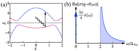
Figure 4: (a) The single particle excitation of the charge $4e$ SC model using the wavefunction method Li et al. (2022). The arrow represents the direct transition between the two bands due to the optical absorption. (b) The complex optical conductance spectrum of the system. The parameters used in the calculation are $m=0.5$, $\mu=2$ and $\Delta_{4e}=1$.

Above results can be further extended to charge $4e$ superconductors Li et al. (2022), where the superfluid density reduced to $3/4$ of that in a two-electron BCS superconductors. Using the wavefunction method Li et al. (2022), we can calculate the Green’s function of charge $4e$ SC as

$$G^{R}(k\sigma,\omega)_{\alpha\alpha} = \frac{u_{k}^{2}}{\omega+\mathrm{i}\eta-(E_{k}-\xi_{k})}+\frac{v_{k}^{2}}{\omega+\mathrm{i}\eta+(E_{k}+\xi_{k})},$$

where $\xi_{k}=\frac{k^{2}}{2m}-\mu$ and $E_{k}=\sqrt{4\xi_{k}^{2}+\Delta_{4e}^{2}}$. The single particle excitation spectrum is shown in Fig.4(a). This spectrum is highly particle-hole asymmetric, since adding one electron and adding one hole are related to different excitation states Li et al. (2022). Through the optical conductance shown in Fig.4(b), we find that finite paramagnetic response corresponding to the direct transition between the two excitations at high frequency leads to a reduction in the superfluid density. Although it stems from the multi-body pairing rather than different-mass Cooper pairs, the reduction of the superfluid stiffness due to finite paramagnetic contribution is a common property in unconventional superconductors.

In summary, we carry out a systematic study of electromagnetic property in superconductors with different-mass Cooper pairs. We find that the different-mass Cooper pairing can result in new paramagnetic contributions in superfluid stiffness. This paramagnetic response directly links to the relative motion between two different mass electrons inside each Cooper pair. Using the two-band model with interband pairing, the paramagnetic responses are calculated based on the linear-response theory from both continuum model and lattice model. This paramagnetic response is finite only at $m_{1}\neq m_{2}$. Furthermore, this reduced superfluid stiffness can be understood from the optical sum rule. The weight from finite $\sigma(\omega\neq 0)$ is equal to this paramagnetic response. Besides the interband pairing in multiband systems, this paramagnetic response also exists in PDW system and other different-mass Cooper pair SCs. Finally, we want to point out this paramagnetic contribution is common both in different-mass Cooper pair systems and multi-body pairing superconducting systems, as we have demonstrated in the charge $4e$ and correlated BCS superconductors Li et al. (2022, 2023). These results offer a new perspective on the superfluid stiffness in superconductors beyond BCS theory.

.1 Acknowledgement

This work is supported by the Ministry of Science and Technology (Grant No. 2022YFA1403901), the National Natural Science Foundation of China (Grant No. NSFC-11888101, No. NSFC-12174428), the Strategic Priority Research Program of the Chinese Academy of Sciences (Grant No. XDB28000000, XDB33000000), the New Cornerstone Investigator Program, and the Chinese Academy of Sciences through the Project for Young Scientists in Basic Research (2022YSBR-048).

Supplemental Material

I superfluid response and optical conductance

The eigenenergy of the Hamiltonian $H_{1}$ (Eq.5) in the main text is

$$E_{k}^{\pm}=\eta_{k}\pm\mathcal{E}_{k}=\eta_{k}\pm\sqrt{\epsilon_{k}^{2}+\Delta^{2}}$$ (S1)

with corresponding eigenvectors $(u_{k},v_{k})^{\mathrm{T}}$ and $(v_{k},-u_{k})^{\mathrm{T}}$ respectively in which

$$u_{k} = \sqrt{\frac{1}{2}\left(1+\frac{\epsilon_{k}}{\mathcal{E}_{k}}\right)}$$ (S2)

$$v_{k} = \sqrt{\frac{1}{2}\left(1-\frac{\epsilon_{k}}{\mathcal{E}_{k}}\right)}$$ (S3)

The Green’s function of the system described by $H_{1}$ can be expressed as

$$\mathcal{G}=\left({\mathrm{i}}\omega_{n}-H_{1}\right)^{-1}\equiv\left(\begin{array}[]{cc}G(k,{\mathrm{i}}\omega_{n})&F(k,{\mathrm{i}}\omega_{n})\\ F^{\dagger}(k,{\mathrm{i}}\omega_{n})&\bar{G}(k,{\mathrm{i}}\omega_{n})\end{array}\right)$$ (S4)

where

$$G(k,{\mathrm{i}}\omega_{n}) = \frac{u_{k}^{2}}{{\mathrm{i}}\omega_{n}-E_{+}}+\frac{v_{k}^{2}}{{\mathrm{i}}\omega_{n}-E_{-}},$$ (S5)

$$\bar{G}(k,{\mathrm{i}}\omega_{n}) = \frac{v_{k}^{2}}{{\mathrm{i}}\omega_{n}-E_{+}}+\frac{u_{k}^{2}}{{\mathrm{i}}\omega_{n}-E_{-}},$$ (S6)

$$F(k,{\mathrm{i}}\omega_{n}) = \frac{u_{k}v_{k}}{{\mathrm{i}}\omega_{n}-E_{+}}-\frac{u_{k}v_{k}}{{\mathrm{i}}\omega_{n}-E_{-}}.$$ (S7)

The paramagnetic current is defined as

$$\hat{J}^{P}_{\mu}(q)=\sum_{\alpha,k}\gamma_{\alpha}(2k+q)_{\mu}c_{k+q,\alpha}^{\dagger}c_{k\alpha}$$ (S8)

which can be decomposed into two components as discussed in the main text: the COM motion and the relative motion,

$$J^{P}(k,q) = J^{P}_{R}+J^{P}_{r}=\frac{\gamma_{1}+\gamma_{2}}{2}(2k+q)\sigma_{0}+\frac{\gamma_{1}-\gamma_{2}}{2}(2k+q)\sigma_{3}$$ (S9)

Then the paramagnetic part of the linear response, i.e. current-current correlation function, can be calculated by

$$\Pi_{\mu\nu}(q,{\mathrm{i}}\Omega_{n}) = \frac{1}{V\beta}\sum_{k,{\mathrm{i}}\omega_{n}}\Tr[J^{P}_{\mu}(q)\mathcal{G}(k,{\mathrm{i}}\omega_{n})J^{P}_{\nu}(q)\mathcal{G}(k+q,{\mathrm{i}}\omega_{n}+{\mathrm{i}}\Omega_{n})]$$ (S10)

$$= (\gamma_{1}+\gamma_{2})^{2}\chi_{00}+2(\gamma_{1}^{2}-\gamma_{2}^{2})\chi_{30}+(\gamma_{1}-\gamma_{2})^{2}\chi_{33}$$ (S11)

where

$$\chi_{ij}(q,{\mathrm{i}}\Omega_{n})=\frac{1}{4V\beta}\sum_{k,{\mathrm{i}}\omega_{n}}(2k+q)_{\mu}(2k+q)_{\nu}\Tr\left[\sigma_{i}\mathcal{G}(k,{\mathrm{i}}\omega_{n})\sigma_{j}\mathcal{G}(k+q,{\mathrm{i}}\omega_{n}+{\mathrm{i}}\Omega_{n})\right].$$ (S12)

Considering the case $T=0$, the results of these correlation functions are

$$\chi_{00}(q,{\mathrm{i}}\Omega_{n}) = \frac{1}{4V}\sum_{k}(2k+q)_{\mu}(2k+q)_{\nu}\left[-\frac{u^{2}\tilde{v}^{2}+v^{2}\tilde{u}^{2}-2uv\tilde{u}\tilde{v}}{{\mathrm{i}}\Omega_{n}+E^{+}-\tilde{E}^{-}}+\frac{\tilde{u}^{2}v^{2}+u^{2}\tilde{v}^{2}-2uv\tilde{u}\tilde{v}}{{\mathrm{i}}\Omega_{n}+E^{-}-\tilde{E}^{+}}\right].$$ (S13)

$$\chi_{33}(q,{\mathrm{i}}\Omega_{n}) = \frac{1}{4V}\sum_{k}(2k+q)_{\mu}(2k+q)_{\nu}\left[-\frac{u^{2}\tilde{v}^{2}+v^{2}\tilde{u}^{2}+2uv\tilde{u}\tilde{v}}{{\mathrm{i}}\Omega_{n}+E^{+}-\tilde{E}^{-}}+\frac{\tilde{u}^{2}v^{2}+u^{2}\tilde{v}^{2}+2uv\tilde{u}\tilde{v}}{{\mathrm{i}}\Omega_{n}+E^{-}-\tilde{E}^{+}}\right].$$ (S14)

$$\chi_{30}(q,{\mathrm{i}}\Omega_{n}) = \frac{1}{4V}\sum_{k}(2k+q)_{\mu}(2k+q)_{\nu}\left[-\frac{u^{2}\tilde{v}^{2}-v^{2}\tilde{u}^{2}}{{\mathrm{i}}\Omega_{n}+E^{+}-\tilde{E}^{-}}+\frac{\tilde{u}^{2}v^{2}-u^{2}\tilde{v}^{2}}{{\mathrm{i}}\Omega_{n}+E^{-}-\tilde{E}^{+}}\right].$$ (S15)

where $u=u_{k}$, $v=v_{k}$, $E^{\pm}=E_{k}^{\pm}$, $\tilde{u}=u_{k+q}$, $\tilde{v}=v_{k+q}$ and $\tilde{E}^{\pm}=E^{\pm}_{k+q}$.

In the long wavelength limit $q\to 0$, we have $\tilde{u}\to u$, $\tilde{v}\to v$ and $\tilde{E}^{\pm}\to E^{\pm}$ and obviously $\chi_{00}=\chi_{30}=0$ and then

$$\real\Pi_{\mu\nu}({\mathrm{i}}\Omega_{n}=0,q\to 0) = -\frac{4}{V}\sum_{k}k_{\mu}k_{\nu}\frac{(\gamma_{1}-\gamma_{2})^{2}u^{2}v^{2}}{\mathcal{E}_{k}}$$ (S16)

$$= -\frac{(\gamma_{1}-\gamma_{2})^{2}}{V}\sum_{k}k_{\mu}^{2}\frac{\Delta^{2}}{\mathcal{E}_{k}^{3}}\delta_{\mu\nu}$$

$$= -\frac{(\gamma_{1}-\gamma_{2})^{2}}{2(\gamma_{1}+\gamma_{2})}\int d\epsilon N_{\gamma^{+}}(\epsilon)\epsilon_{F}\frac{\Delta^{2}}{(\epsilon^{2}+\Delta^{2})^{3/2}}\delta_{\mu\nu}$$

$$= -\frac{(\gamma_{1}-\gamma_{2})^{2}\epsilon_{F}N_{\gamma^{+}}(0)}{\gamma_{1}+\gamma_{2}}\delta_{\mu\nu}$$

where $N_{\gamma_{1}+\gamma_{2}}$ is the DOS of the 2D free electron gas with energy dispersion $(\gamma_{1}+\gamma_{2})k^{2}$, which is proportional to $\frac{1}{\gamma_{1}+\gamma_{2}}$. If $\gamma_{1}=\gamma_{2}$, the paramagnetic contrition vanishes which is just the single band case. This result suggests that the nonzero paramagnetic contribution stems from interband pairing.

Then we shall consider the diamagnetic contribution. The diamagnetic current is defined as

$$J^{D}_{\mu}=\sum_{k\alpha}\frac{e^{2}\hat{n}_{\alpha,\mu\nu}}{m_{\alpha}}A_{\nu}$$ (S17)

The matrix form is

$$J^{D}(q)=\left(\begin{array}[]{cc}2\gamma_{1}&0\\ 0&-2\gamma_{2}\end{array}\right)=J^{D}_{R}+J^{D}_{r}=(\gamma_{1}+\gamma_{2})\sigma_{3}+(\gamma_{1}-\gamma_{2})\sigma_{0}$$ (S18)

Thus the diamagnetic contribution of superfluid stiffness can be obtained by calculating

$$\left<\bf{J}^{D}\right> = \frac{1}{V\beta}\sum_{k,{\mathrm{i}}\omega_{n}}\Tr\left[J^{D}\mathcal{G}(k,{\mathrm{i}}\omega_{n})\right]\bf{A}$$ (S19)

$$= \sum_{k}(\gamma_{1}+\gamma_{2})\left[1-\frac{\epsilon_{k}}{\mathcal{E}_{k}}\left[n_{F}(E_{k}^{-})-n_{F}(E_{k}^{+})\right]\right]-\sum_{k}(\gamma_{1}-\gamma_{2})\left[1-\left[n_{F}(E_{k}^{-})-n_{F}(E_{k}^{+})\right]\right]\bf{A}$$

$$\xlongequal{T=0} \sum_{k}(\gamma_{1}+\gamma_{2})\left[1-\frac{\epsilon_{k}}{\mathcal{E}_{k}}\right]\bf{A}$$

$$= (\gamma_{1}+\gamma_{2})n_{c}\bf{A}$$

where $n_{c}$ is the number of carriers in either band.

Below we shall calculate the optical conductance and check the optical sum rule

$$\imaginary\Pi_{\mu\nu}(\Omega,q\to 0) = -\frac{\pi}{V}\sum_{k}k_{\mu}^{2}\frac{(\gamma_{1}-\gamma_{2})^{2}\Delta^{2}}{\mathcal{E}_{k}^{2}}\left[\delta(\Omega+2\mathcal{E}_{k})-\delta(\Omega-2\mathcal{E}_{k})\right]\delta_{\mu\nu}$$ (S20)

$$= -\frac{\pi(\gamma_{1}-\gamma_{2})^{2}\epsilon_{F}N_{\gamma^{+}}(0)}{2(\gamma_{1}+\gamma_{2})}\int d\epsilon\frac{\Delta^{2}}{\epsilon^{2}+\Delta^{2}}\left[\delta\left(\Omega+2\sqrt{\epsilon^{2}+\Delta^{2}}\right)-\delta\left(\Omega-2\sqrt{\epsilon^{2}+\Delta^{2}}\right)\right]\delta_{\mu\nu}$$

Using the property of $\delta$-function $\delta\left[g(\epsilon)\right]=\sum_{i}\frac{\delta(\epsilon-\epsilon_{i})}{\absolutevalue{g^{\prime}(\epsilon_{i})}}$, we have

$$\int d\epsilon\frac{\Delta^{2}}{\epsilon^{2}+\Delta^{2}}\delta\left(\Omega-2\sqrt{\epsilon^{2}+\Delta^{2}}\right) = \int d\epsilon\frac{\Delta^{2}}{\epsilon^{2}+\Delta^{2}}\left[\frac{\delta\left(\epsilon-\frac{1}{2}\sqrt{\Omega^{2}-4\Delta^{2}}\right)}{2\sqrt{\Omega^{2}-4\Delta^{2}}/\Omega}+\frac{\delta\left(\epsilon+\frac{1}{2}\sqrt{\Omega^{2}-4\Delta^{2}}\right)}{2\sqrt{\Omega^{2}-4\Delta^{2}}/\Omega}\right]$$ (S21)

$$= \frac{4\Delta^{2}}{\Omega\sqrt{\Omega^{2}-4\Delta^{2}}},\quad(\Omega>0)$$

Since $\imaginary\Pi_{\mu\nu}(\Omega,q\to 0)$ is odd function of $\Omega$, the integration of it is

$$\int_{-\infty}^{\infty}d\Omega\frac{\imaginary\Pi_{\mu\nu}(\Omega,q\to 0)}{\Omega} = 2\int_{0}^{\infty}d\Omega\frac{\imaginary\Pi_{\mu\nu}(\Omega,q\to 0)}{\Omega}$$ (S22)

$$= \frac{\pi(\gamma_{1}-\gamma_{2})^{2}\epsilon_{F}N_{\gamma^{+}}(0)}{\gamma_{1}+\gamma_{2}}\delta_{\mu\nu}\int_{2\Delta}^{\infty}d\Omega\frac{4\Delta^{2}}{\Omega^{2}\sqrt{\Omega^{2}-4\Delta^{2}}}$$

$$= \frac{\pi(\gamma_{1}-\gamma_{2})^{2}\epsilon_{F}N_{\gamma^{+}}(0)}{\gamma_{1}+\gamma_{2}}\delta_{\mu\nu}$$

$$= \pi\real\Pi_{\mu\nu}(\Omega=0,q\to 0)$$

Thus the optical sum rule is satisfied.

The real part of optical conductance is

$$\real\sigma_{\mu\mu}(q\to 0,\Omega>0)=\frac{\imaginary\Pi_{\mu\nu}(\Omega,q\to 0)}{\Omega}=\frac{4\pi(\gamma_{1}-\gamma_{2})^{2}\Delta^{2}\epsilon_{F}N_{\gamma^{+}}(0)}{2(\gamma_{1}+\gamma_{2})\Omega^{2}\sqrt{\Omega^{2}-4\Delta^{2}}}$$ (S23)

which is showed in Fig.2(d).

II Two different-mass bands with the same Fermi surface

In our main text, the two different-mass bands have a degeneracy at the band bottom, resulting in separated Fermi surfaces. Consequently, the interband pairing order parameter needs to exceed a critical value for the system to be fully gapped. Actually, the bottom of the two bands may not be degenerate, allowing their Fermi surfaces to coincide. That means the two bands hosts the dispersion with different Fermi energy $\xi_{\alpha}(k)=\frac{k^{2}}{2m_{\alpha}}-\mu_{\alpha}$. By tuning $\mu_{1}/\mu_{2}=\gamma_{1}/\gamma_{2}$, we can get this case as shown in Fig.S1(a). Due to the perfectly nesting Fermi surface of the two bands, infinitesimal interband pairing order parameter can make the system fully gapped as shown in Fig.S1(b).

We find that in this case, the eigenvalue of $H_{1}$ are $E_{k}^{\pm}=\eta_{k}\pm\sqrt{\epsilon_{k}^{2}+\Delta^{2}}$, where $\eta_{k}=\frac{\gamma_{1}-\gamma_{2}}{2}k^{2}-\frac{\mu_{1}-\mu_{2}}{2}$ and $\epsilon_{k}=\frac{\gamma_{1}+\gamma_{2}}{2}k^{2}-\frac{\mu_{1}+\mu_{2}}{2}$. It is a little different from the case in the main text, but the result of superfuild response is the same.

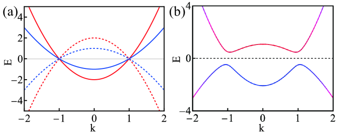
Figure S1: (a) The energy of the two bands with different mass and the same Fermi surface. The dashed line is the particle-hole symmetric band. (b) The band structure of the two different-mass band superconductor with inter-band pairing. The parameters used in the calculation are $\gamma_{1}=2$, $\gamma_{2}=1$, $\mu_{1}=2$, $\mu_{2}=1$ and $\Delta=0.5$.

III Quasiparticle band of PDW

We plot the quasiparticle band of the $Q=(\pi,\pi)$ PDW in Fig.S2(b) along the high symmetric line shown in Fig.S2(a). The optical transition process is similar to that of the interband pairing SC with different mass Cooper pairs.

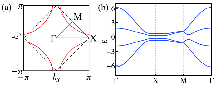
Figure S2: (a) The first Brillouin zone (BZ) of the square lattice. Red lines show the Fermi surface of $\xi_{k}$. Dashed lines are the reduced BZ. Blue lines are the high symmetry line. (b) The quasiparticle band of the Hamiltonian Eq.7 along the high symmetry line. The order parameter is set as $\Delta_{on}=0.5$ and $\Delta_{PDW}=0.2$.

IV superfluid response and optical conductance of the charge 4$e$ SC

Following the paper Li et al. (2022), the current operator matrix under the basis $\left(c_{1\bm{k}\uparrow},\;c_{2\bm{k}\uparrow},\;c_{1-\bm{k}\downarrow}^{\dagger},\;c_{2-\bm{k}\downarrow}^{\dagger}\right)^{\mathrm{T}}$ can be written as

$$J^{P}(k,q)=\frac{2k+q}{2m}\tau_{0}\sigma_{0}$$ (S24)

where $\tau$ and $\sigma$ are Pauli matrix in particle-hole and orbital space respectively. The single particle Green’s function has the form

$$\bar{G}^{R}(\bm{k},{\mathrm{i}}\omega_{n})=\left(\begin{array}[]{cccc}\frac{\omega+{\mathrm{i}}\eta+3\xi_{{\bf k}}}{(\omega+{\mathrm{i}}\eta+\xi_{{\bf k}})^{2}-E_{{\bf k}}^{2}}&&&\\ &\frac{\omega+{\mathrm{i}}\eta+3\xi_{{\bf k}}}{(\omega+{\mathrm{i}}\eta+\xi_{{\bf k}})^{2}-E_{{\bf k}}^{2}}&&\\ &&\frac{\omega+{\mathrm{i}}\eta-3\xi_{{\bf k}}}{(\omega+{\mathrm{i}}\eta-\xi_{{\bf k}})^{2}-E_{{\bf k}}^{2}}&\\ &&&\frac{\omega+{\mathrm{i}}\eta-3\xi_{{\bf k}}}{(\omega+{\mathrm{i}}\eta-\xi_{{\bf k}})^{2}-E_{{\bf k}}^{2}}\end{array}\right).$$ (S25)

Then the current-current correlation function can be calculated via Eq.S10 and the result at zero temperature are

$$\real\Pi_{\mu\mu}({\mathrm{i}}\Omega_{n}=0,q\to 0)=\frac{\epsilon_{F}N(\epsilon_{F})}{6m}$$ (S26)

$$\imaginary\Pi_{\mu\mu}(\Omega,q\to 0)=\frac{\pi\epsilon_{F}N(\epsilon_{F})}{3m}\frac{\Delta^{2}}{\Omega\sqrt{\Omega^{2}-4\Delta^{2}}}$$ (S27)

Thus, the superfluid density is obtained as

$$\rho_{s}={\langle}\frac{n}{m}{\rangle}-\real\Pi_{\mu\mu}({\mathrm{i}}\Omega_{n}=0,q\to 0)=\frac{3\rho}{4}$$ (S28)

where $\rho=\frac{2\epsilon_{F}N(\epsilon_{F})}{3m}$, and the real part of the optical conductance is

$$\real\sigma_{\mu\mu}(q\to 0,\Omega>0)=\frac{\imaginary\Pi_{\mu\nu}(\Omega,q\to 0)}{\Omega}=\frac{\pi\epsilon_{F}N(\epsilon_{F})}{3m}\frac{\Delta^{2}}{\Omega^{2}\sqrt{\Omega^{2}-4\Delta^{2}}}$$ (S29)

It’s straightforward to check that the optical sum rule is satisfied.

References

Schrieffer (1964)J.R. Schrieffer, Theory of
Superconductivity (Addison-Wesley, Reading, MA, 1964).
Bardeen et al. (1957)J. Bardeen, L. N. Cooper,
and J. R. Schrieffer, “Theory of
superconductivity,” Phys. Rev. 108, 1175–1204 (1957).
Coleman (2015)Piers Coleman, Introduction to
many-body physics (Cambridge University Press, 2015).
Scalapino et al. (1993)Douglas J. Scalapino, Steven R. White, and Shoucheng Zhang, “Insulator, metal, or superconductor: The criteria,” Phys.
Rev. B 47, 7995–8007
(1993).
Xiang and Wu (2022)Tao Xiang and Congjun Wu, D-wave Superconductivity (Cambridge University Press, 2022).
Uemura et al. (1993)Y. J. Uemura, A. Keren,
L. P. Le, G. M. Luke, W. D. Wu, Y. Kubo, T. Manako, Y. Shimakawa,
M. Subramanian, J. L. Cobb, and J. T. Markert, “Magnetic-field penetration depth in
ti2ba2cuo6+ in the overdoped regime,” Nature 364, 605–607 (1993).
Božović et al. (2016)I. Božović, X. He, J. Wu, and A. T. Bollinger, “Dependence of the critical
temperature in overdoped copper oxides on superfluid density,” Nature 536, 309–311
(2016).
Mahmood et al. (2019)Fahad Mahmood, Xi He,
Ivan Božović, and N. P. Armitage, “Locating the missing
superconducting electrons in the overdoped cuprates
,” Phys. Rev. Lett. 122, 027003 (2019).
Lee-Hone et al. (2020)N. R. Lee-Hone, H. U. Özdemir, V. Mishra,
D. M. Broun, and P. J. Hirschfeld, “Low energy phenomenology of
the overdoped cuprates: Viability of the landau-bcs paradigm,” Phys. Rev. Res. 2, 013228 (2020).
Wang et al. (2022)Da Wang, Jun-Qi Xu,
Hai-Jun Zhang, and Qiang-Hua Wang, “Anisotropic scattering
caused by apical oxygen vacancies in thin films of overdoped high-temperature
cuprate superconductors,” Phys. Rev. Lett. 128, 137001 (2022).
Li et al. (2021)Zi-Xiang Li, Steven A. Kivelson, and Dung-Hai Lee, “Superconductor-to-metal transition in overdoped cuprates,” npj Quantum Materials 6, 36 (2021).
Suhl et al. (1959)H. Suhl, B. T. Matthias,
and L. R. Walker, “Bardeen-cooper-schrieffer
theory of superconductivity in the case of overlapping bands,” Phys. Rev. Lett. 3, 552–554 (1959).
Agterberg et al. (2020a)Daniel F. Agterberg, J.C. Séamus Davis, Stephen D. Edkins, Eduardo Fradkin, Dale J. Van Harlingen, Steven A. Kivelson, Patrick A. Lee, Leo Radzihovsky, John M. Tranquada, and Yuxuan Wang, “The
physics of pair-density waves: Cuprate superconductors and beyond,” Annual Review of Condensed Matter Physics 11, 231–270 (2020a).
Shen et al. (1965)Lawrence Yun Lung Shen, N. M. Senozan, and Norman E. Phillips, “Evidence for
two energy gaps in high-purity superconducting nb, ta, and v,” Phys. Rev. Lett. 14, 1025–1027 (1965).
Blackford and March (1969)B. L. Blackford and R. H. March, “Tunneling
investigation of energy-gap anisotropy in superconducting bulk pb,” Phys. Rev. 186, 397–399 (1969).
Souma et al. (2003)S. Souma, Y. Machida,
T. Sato, T. Takahashi, H. Matsui, S. C. Wang, H. Ding, A. Kaminski, J. C. Campuzano, S. Sasaki, and K. Kadowaki, “The origin of multiple
superconducting gaps in mgb2,” Nature 423, 65–67 (2003).
Schooley et al. (1964)J. F. Schooley, W. R. Hosler, and Marvin L. Cohen, “Superconductivity
in semiconducting srti,” Phys.
Rev. Lett. 12, 474–475
(1964).
Takahashi et al. (2008)Hiroki Takahashi, Kazumi Igawa, Kazunobu Arii,
Yoichi Kamihara, Masahiro Hirano, and Hideo Hosono, “Superconductivity at 43 k in an iron-based
layered compound ,” Nature 453, 376–378 (2008).
Paglione and Greene (2010)Johnpierre Paglione and Richard L. Greene, “High-temperature superconductivity in iron-based materials,” Nature Physics 6, 645–658 (2010).
Ferrell and Glover (1958)Richard A. Ferrell and Rolfe E. Glover, “Conductivity of superconducting films: A sum rule,” Phys.
Rev. 109, 1398–1399
(1958).
Tinkham and Ferrell (1959)M. Tinkham and R. A. Ferrell, “Determination
of the superconducting skin depth from the energy gap and sum rule,” Phys. Rev. Lett. 2, 331–333 (1959).
Ahn and Nagaosa (2021)Junyeong Ahn and Naoto Nagaosa, “Theory of optical responses in clean multi-band superconductors,” Nature Communications 12, 1617 (2021).
Cvetkovic and Vafek (2013)Vladimir Cvetkovic and Oskar Vafek, “Space group symmetry, spin-orbit coupling, and the low-energy effective
hamiltonian for iron-based superconductors,” Phys.
Rev. B 88, 134510
(2013).
Chen et al. (2021)Hui Chen, Haitao Yang,
Bin Hu, Zhen Zhao, Jie Yuan, Yuqing Xing, Guojian Qian, Zihao Huang, Geng Li,
Yuhan Ye, Sheng Ma, Shunli Ni, Hua Zhang, Qiangwei Yin, Chunsheng Gong, Zhijun Tu, Hechang Lei,
Hengxin Tan, Sen Zhou, Chengmin Shen, Xiaoli Dong, Binghai Yan, Ziqiang Wang, and Hong-Jun Gao, “Roton pair density wave in a strong-coupling
kagome superconductor,” Nature 599, 222–228 (2021).
Edkins et al. (2019)S. D. Edkins, A. Kostin,
K. Fujita, A. P. Mackenzie, H. Eisaki, S. Uchida, Subir Sachdev, Michael J. Lawler, E.-A. Kim, J. C. Séamus Davis, and M. H. Hamidian, “Magnetic field–induced pair density wave state in the cuprate vortex
halo,” Science 364, 976–980 (2019), https://www.science.org/doi/pdf/10.1126/science.aat1773 .
Hamidian et al. (2016)M. H. Hamidian, S. D. Edkins, Sang Hyun Joo,
A. Kostin, H. Eisaki, S. Uchida, M. J. Lawler, E. A. Kim, A. P. Mackenzie, K. Fujita,
Jinho Lee, and J. C. Séamus Davis, “Detection of a cooper-pair
density wave in bi2sr2cacu2o8+x,” Nature 532, 343–347 (2016).
Ruan et al. (2018)Wei Ruan, Xintong Li,
Cheng Hu, Zhenqi Hao, Haiwei Li, Peng Cai, Xingjiang Zhou, Dung-Hai Lee, and Yayu Wang, “Visualization of the periodic modulation of cooper pairing in a cuprate
superconductor,” Nature Physics 14, 1178–1182 (2018).
Lee (2014)Patrick A. Lee, “Amperean pairing and the pseudogap phase of cuprate superconductors,” Phys. Rev. X 4, 031017 (2014).
Li et al. (2022)Pengfei Li, Kun Jiang, and Jiangping Hu, “Charge 4 superconductor: a
wavefunction approach,” arXiv preprint arXiv:2209.13905 (2022).
Li et al. (2023)Pengfei Li, Kun Jiang, and Jiangping Hu, “Correlated bcs wavefunction approach to
unconventional superconductors,” arXiv preprint arXiv:2309.02695 (2023).