Scheduling and Communication Schemes for Decentralized Federated Learning

Abstract

Federated learning (FL) is a distributed machine learning paradigm in which a large number of clients coordinate with a central server to learn a model without sharing their own training data. One central server is not enough, due to problems of connectivity with clients. In this paper, a decentralized federated learning (DFL) model with the stochastic gradient descent (SGD) algorithm has been introduced, as a more scalable approach to improve the learning performance in a network of agents with arbitrary topology. Three scheduling policies for DFL have been proposed for communications between the clients and the parallel servers, and the convergence, accuracy, and loss have been tested in a totally decentralized implementation of SGD. The experimental results show that the proposed scheduling polices have an impact both on the speed of convergence and in the final global model.

I Introduction

Data generated at device terminals has recently increased exponentially, owing to the explosive growth of powerful individual computing devices worldwide and the rapid advancement of the Internet of Things (IoT). Data-driven machine learning is becoming a popular technique for making predictions and decisions about future events by making full use of massive amounts of data. Federated Learning (FL), a promising data-driven machine learning variant, provides a communication-efficient approach for processing large amounts of distributed data and is gaining popularity.FL was first proposed as a critical technique of distributed machine learning in a centralised form, in which edge clients perform local model training in parallel and a central server aggregates the trained model parameters from the edge without transmitting raw data from the edge clients to the central server.

FL was first tested on a Google Android keyboard (Gboard). It supports multilingual typing, including Google searches and sharing results from the keyboard, as well as auto-correction, voice typing, and glide typing. When Gboard displays some suggestions on the screen based on user behavior, local learning occurs, and FL gains sway by improving future suggestions/interactions with the user. As a result, improved features such as next-word prediction, word completion, corrections, and many more are available. To implement and experiment FL on decentralized data, the following open-source frameworks are in development/available: TensorFlow Federated (TFF) [1], Federated AI Technology Enabler (FATE) [2], PySyft [3], PaddleFL [4], Clara Training Framework [5].

FL plays a crucial role in supporting the privacy protection of user data and deploying in a complex environment with massive intelligent terminal access to the network center due to the property of transmitting model parameters instead of user data and the distributed network structure that an arbitrary number of edge nodes are coordinated through one central server. FL operates as a centralized model with decentralized data, which makes the central server a critical point of failure. Besides, in many cases of interest, not every client has a direct connection to the server for learning of the global model [6].

Decentralized Federated Learning (DFL) is therefore well suited to implement distributed learning with multiple data aggregators, thus reducing the cost of communication and the workload of the central server. DFL has been proposed and analyzed in the literature under specific updating algorithms in the distributed servers (see [7, 8, 9], but these works rely on a strict and rigid strategy for the update and communication phases of the protocol. This might be difficult to achieve in general networks, where density and asymmetry are frequent. Consequently, the impact of the scheduling policy between the nodes acting as clients and the servers is a complex decision affecting the global behavior of learning algorithm.

In this work, scheduling policies have been proposed for DFL designed to get insights about convergence, loss, and accuracy. The paper is organized as follows. In Section II, the related work is introduced. Next, Section III presents the proposed DFL system model and the main assumptions. The experimental results are presented and discussed in Section IV, and finally conclusions appear in Section V.

II Related Work

Numerous authors have discussed and created solutions for problems with FL resource allocation in their writings. The FL problem over wireless networks formulated in [10] captures the following trade-offs : (1) using the Pareto efficiency model, measuring learning time in relation to customer energy use, and (2) computation versus communication learning time by determining the ideal learning accuracy. In [11], by developing a joint bandwidth allocation and scheduling issue to reduce training time and achieve the desired model accuracy, the authors suggest a method for increasing the convergence rate of FL training concerning time. For the bandwidth allocation problem, they design an efficient binary search algorithm, while for maximum device scheduling, they adopt a greedy approach for achieving a trade-off between the latency and learning efficiency in each round. In [12], The authors define the joint learning, wireless resource allocation, and client selection problem as an optimization problem to minimize the FL loss function. In [13], the authors describe a method for self-organizing FL over wireless networks. They use a heuristic algorithm to minimize global FL time while taking local energy consumption and resource blocks into account.

IN [14], the authors suggests a paradigm for evaluating and describing FL performance. For the convergence rate of FL, traceable expressions are generated that consider the impact of inter-cell interference as well as scheduling strategies. They also looked at the efficiency (convergence rate) of scheduling rules such as proportional fair scheduling, round robin scheduling, and random scheduling. Other works have begun examining scheduling strategies influenced by the chances for model improvement during FL rounds. According to the channel circumstances and the importance of local model updates, [15] establishes scheduling policies for selecting the subset of devices to handle the transmission inside each round.

In wireless networks with clients sharing a single wireless link, the contribution of [16] offers a long-term perspective for resource allocation. The method is grounded in experimental observation showing that choosing fewer customers during the initial learning rounds and then gradually increasing this number is the strategy having the best impact on learning performance. In [17], the clients are divided into tiers according to how well they performed during training, and an adaptive tier-based client selection method is used in the authors’ proposed Tier-based Federated Learning (TEFL) System. In [18], it is suggested a scheduling strategy to make use of variation in multi-user channels as well as diversity in the significance of edge device learning updates (measured by gradient divergence). In [19], the authors propose a proactive algorithm that selects mobile clients based on predictions of their future training and reporting abilities. The adopted approach is divided into two parts: (1) In a metropolitan mobile edge computing environment, predicting users’ mobility trajectory patterns and the apps they use on their smartphones, as well as (2) a deep reinforcement learning-based client-selection algorithm handling unanticipated dynamic events, are all possible. CPU, bandwidth, GPS coordinates, and the success or failure of downloading and uploading local and global parameters are the metrics that are observed and forecast.

The authors at [20] advocate the decentralized approach that leaves the training data distributed on the edge devices and learns a shared model by aggregating locally computed updates. They show a practical method for FL of deep networks based on iterative model averaging, and conduct an extensive empirical evaluation, considering five different model architectures and four datasets. The Decentralized SGD is a driving engine for FL and its performance is influenced by internode communications and local updates. At [21] propose a DFL framework that implements both internode communication periodically and multiple local updates to strike a balance between communication efficiency and model consensus. They establish strong convergence guarantees for the DFL algorithm without the assumption of convex objects.

III Model of Peer-to-Peer Decentralized FL

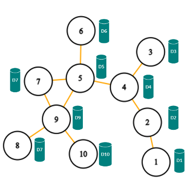
Figure 1: System Model for Decentralized Federated Learning.

TABLE I: Scheduling policies for the decentralized learning algorithm.

	scheduler a	scheduler b	scheduler c
Rounds $t=2k+1$	$\{2,3\}\to 4$, $\{6,7\}\to 5$, $\{8,10\}\to 9$	$\{2,3\}\to 4$, $\{6\}\to 5$, $\{7,8,10\}\to 9$	$\{2,3\}\to 4$, $\{8,10\}\to 9$
Rounds $t=2k$	$\{4,9\}\to 5$, $\{1\}\to 2$	$\{4,9\}\to 5$, $\{1\}\to 2$	$\{4,6,7,9\}\to 5$, $\{1\}\to 2$

The graph, the scheduler, and the global parameters aggregation are the three parts of the system model that are defined in this section.the first part explains how edge devices in the graph are connected to one another. the second scheduler plans the aggregators and clients. the third part is the aggregator way will combine the parameters given in the aggregation section as well as the specifics of how the new global model parameters will be calculated using FedAvg.

III-A Graph

We consider a community of learning nodes modeled as an undirected graph $G=(V,E)$ with $n=|V|$ nodes. For $i,j\in V$, edge $(i,j)\in E$ represents a bidirectional communication link between nodes $i$ and $j$. Each node is assumed to have access to a local dataset $D_{i},i\in V$, containing $d_{i}=|Di|$ samples of a common unknown distribution D from which we are interested in learning, i.e., in building a statistical model $F_{\boldsymbol{\theta}}$ from a given class, where $\boldsymbol{\theta}$ denotes the model parameters which are to be optimized during the learning process. For instance, $F_{\boldsymbol{\theta}}$ can be a (deep) neural network, and $\boldsymbol{\theta}$ the weights between its adjacent layers. Different from centralized and federated learning (FL), where only a single node is in charge of building $F_{\boldsymbol{\theta}}$, in decentralized or distributed learning (DL) we allow each node to learn from its neighbors, possibly in an asynchronous way.

III-B Schedulers

The scheduler role is choosing which node will work as an aggregator for the parameters from specific neighbors. We propose, for the graph depicted in Figure 1, the three scheduling policies listed in Table I. The notation $\{X,Y\}\to Z$ is used to denote that nodes $X$ and $Y$ are clients and node Z is aggregation node. The criteria for choosing a node to work as an aggregator is based on the round number and it is expressed by the formula Rounds $t=2k+1$ for odd rounds, Rounds $t=2k$ for even rounds.

We see at Table I, for instance, that node $5$ aggregates weights each round in scheduler A. This node was crucial in this scheduler since it aggregates from the other aggregators, so it will hold the most recent model that was averaged across multiple nodes.in every scheduler, the sequence of communications between clients and servers yields, after a pair of rounds, a connected graph.

III-C Decentralized Federated Averaging

Figure 2: Tracking Models for first two rounds for Scheduler A.

The FedAvg Algorithm is the most widely used technique for calculating the global model parameters. We anticipate that the aggregators’ average model will satisfy full convergence. McMahan [20] proposed FedAvg, in which clients collaboratively send updates of locally trained models to the aggregator node, each client running a local copy of the global model on its local trainning data. The global model weights are then updated with an average of the updates from clients and deployed back to clients. This extends previous training work by not only supplying local models but also performing training on each device locally. As a result, FedAvg may enable clients (particularly those with small datasets) to collaboratively learn a shared prediction model while retaining all training data locally. before aggregators construct the global model. neighbors send new model parameters and old global parameters that were kept from previous rounds. The aggregator sums new parameters and old global parameters from itself and the received from neighbors ,then calculate the average to build the new global parameters by using FedAvg. If any node did not participate in any previous rounds, it will send only new local parameters to the aggregator. as it will not have old global parameters. Fig 2 Aggregator nodes are coloured blue in the first round and red in the second. In the first and second rounds, we concentrate on node 5. In the first round, node 5 will aggregate weights from neighbors as well as the old global model four GM4. Node 4 created GM4 while acting as an aggregator. After which a new global model was calculated The new global model is known as GM5, which stands for Global model for node 5. In the second round of GM5, weights from neighbors are added to the old global models from previous rounds. The total will be divided by the number of models. The same criteria will be used in subsequent odd and even rounds.

Pseudo code 1 for each round there are one aggregator and set of clients. When the round starts the aggregator will initialize the clients with random weights . clients will get the random weights or last round weights that are kept from the aggregator. clients and their aggregator will start executing local computations for epochs. the updates will be sent to the aggregator. The aggregator will combine clients updates with its update then generate new parameters using FedAvg. The new parameters will be sent to clients and each client will save it locally . Clients will use global parameters to initiate their clients when they work as aggregators.after round finished the algorithm extracts a new aggregator. the aggregators determined by schedulers.

Algorithm 1 Decentralized FedAVg.

1:while $Q$ is not empty do

2:     for each round $t=1,2\dots$ do

3:         $AG\leftarrow\text{Dequeue(Q) }$ $\triangleright$ extract a new node to work as aggregator from queue

4:         $N\leftarrow\text{set of neighbors/clients of Aggregator (AG)}$

5:         if $w_{t-1}$ Exist then

6:              $\mathbf{w}_{t}\leftarrow\mathbf{w}_{t-1}$$\triangleright$ set initial weights with last round weights aggregated

7:         else

8:              $\mathbf{w}_{t}\leftarrow\mathbf{w}_{0}$$\triangleright$ set initial weights randomly

9:         end if

10:         $AddNeighbour(N,AG)$ $\triangleright$ add aggregator node to neighbor set

11:         for each neighbour $X$ in $N$ do

12:              $\mathbf{w}^{d}_{t+1}\leftarrow\mathsf{NeighborUpdate}(d,\mathbf{w}_{t})$

13:              $\mathbf{w}_{t+1}\leftarrow\sum_{i=1}^{|N_{x}|}\frac{n_{i}}{n}\mathbf{w}_{t+1}^{k}$

14:         end for

15:     end for

16:end while

IV Experimental Results

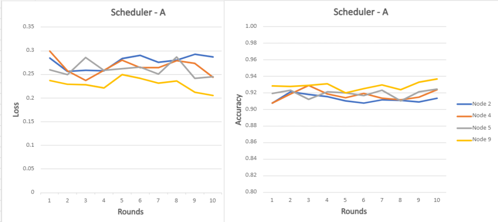
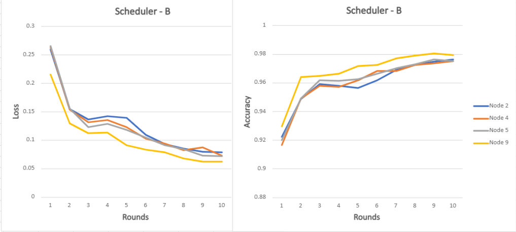
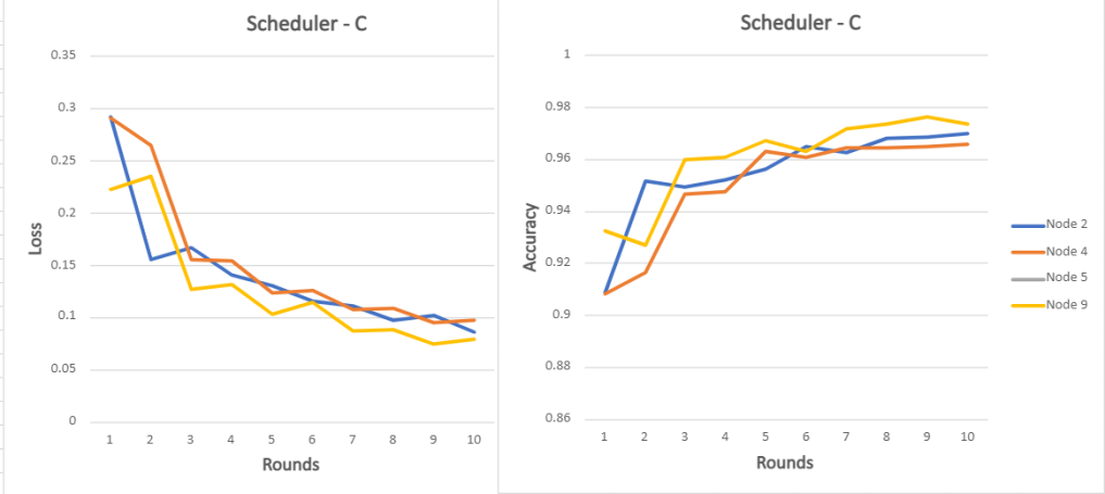
Figure 3: Performance Across Schedulers and Nodes in the graph.

IV-A Environment

IV-A1 Flwr

The implementation was developed under an Flwr environment with anaconda with python. The Project itself contains one python code. When this code is executed the graph description is read. working on Flwr gives the flexibility to simulate real-world scenarios as we need to simulate the communication noise between nodes, and it can work in simulation mode which is very good at simulating nodes to get results quickly.

IV-A2 Google Colab

Google-colab is an online website that we can use to run machine learning model notebooks in the cloud. It provides a good GPU and CPU to run ML notebooks smoothly and get results and save outputs so easily.

IV-A3 WandB

WandB is abbreviated for weight and bias [22] it is an online API that is used with our ML Project for teaching and logging results in an interactive way. It is a very helpful tool for good visualizations and creating reports and notes for any ML Model and tracking parameters, supports many formats and representations to download or view results.

IV-A4 MNIST

The Modified National Institute of Standards and Technology for handwritten digits was used in our experiment to assess the proposed Decentralized FL.

IV-B Results

TABLE II: Loss and accuracy for the network graph and scheduler A and B, per round of learning.

	scheduler a				scheduler b
round	node 2	node 4	node 5	node 9	node 2	node 4	node 5	node 9
$1$	$(0.29,91\%)$	$(0.3,92\%)$	$(0.26,92\%)$	$(0.24,93\%)$	$(0.26,92\%)$	$(0.26,92\%)$	$(0,27,92\%)$	$(0.22,93\%)$
$2$	$\mathbf{(0.26,92\%)}$	$(0.26,92\%)$	$\mathbf{(0.25,92\%)}$	$(0.23,93\%)$	$(0.15,95\%)$	$(0.15,95\%)$	$(0.16,95\%)$	$(0.13,96\%)$
$3$	$\mathbf{(0.26,92\%)}$	$\mathbf{(0.24,93\%)}$	$(0.29,91\%)$	$(0.23,93\%)$	$(0.14,96\%)$	$(0.13,96\%)$	$(0.12,96\%)$	$(0.11,97\%)$
$4$	$\mathbf{(0.26,92\%)}$	$(0.26,92\%)$	$(0.26,92\%)$	$(0.22,93\%)$	$(0.14,96\%)$	$(0.14,96\%)$	$(0.13,96\%)$	$(0.11,97\%)$
$5$	$(0.28,91\%)$	$(0.28,91\%)$	$(0.26,92\%)$	$(0.25,92\%)$	$(0.14,96\%)$	$(0.12,96\%)$	$(0.12,96\%)$	$(0.09,97\%)$
$6$	$(0.29,91\%)$	$(0.26,92\%)$	$(0.27,92\%)$	$(0.24,93\%)$	$(0.11,96\%)$	$(0.1,97\%)$	$(0.1,97\%)$	$(0.08,97\%)$
$7$	$(0.28,91\%)$	$(0.26,91\%)$	$\mathbf{(0.25,92\%)}$	$(0.23,93\%)$	$(0.09,97\%)$	$(0.09,97\%)$	$(0.09,97\%)$	$(0.08,98\%)$
$8$	$(0.28,91\%)$	$(0.28,91\%)$	$(0.29,91\%)$	$(0.24,92\%)$	$(0.09,97\%)$	$(0.08,97\%)$	$(0.08,97\%)$	$(0.07,98\%)$
$9$	$(0.29,91\%)$	$(0.27,92\%)$	$(0.24,92\%)$	$(0.21,93\%)$	$(0.08,97\%)$	$(0.09,97\%)$	$\mathbf{(0.07,98\%)}$	$\mathbf{(0.06,98\%)}$
$10$	$(0.29,91\%)$	$(0.24,92\%)$	$\mathbf{(0.25,92\%)}$	$\mathbf{(0.21,94\%)}$	$\mathbf{(0.08,98\%)}$	$\mathbf{(0.07,98\%)}$	$\mathbf{(0.07,98\%)}$	$\mathbf{(0.06,98\%)}$

TABLE III: Loss and accuracy for the network graph and scheduler C, per round of learning.

round	node 2	node 4	node 5	node 9
$1$	$(0.29,91\%)$	$(0.29,91\%)$	—	$(0.22,93\%)$
$2$	$(0.16,95\%)$	$(0.27,92\%)$	$(0.28,91\%)$	$(0.23,93\%)$
$3$	$(0.17,95\%)$	$(0.16,95\%)$	—	$(0.13,96\%)$
$4$	$(0.14,95\%)$	$(0.15,95\%)$	$(0.16,95\%)$	$(0.13,96\%)$
$5$	$(0.13,96\%)$	$(0.12,96\%)$	—	$(0.1,97\%)$
$6$	$(0.12,97\%)$	$(0.13,96\%)$	$(0.13,96\%)$	$(0.11,96\%)$
$7$	$(0.11,96\%)$	$(0.11,96\%)$	—	$(0.09,97\%)$
$8$	$(0.1,97\%)$	$(0.11,96\%)$	$(0.11,96\%)$	$(0.09,97\%)$
$9$	$(0.1,97\%)$	$(0.1,96\%)$	—	$\mathbf{(0.08,98\%)}$
$10$	$\mathbf{(0.09,97\%)}$	$\mathbf{(0.1,97\%)}$	$\mathbf{(0.1,97\%)}$	$(0.08,97\%)$

[23] has many advantages like stability and the capability of operating in real federated learning scenarios. Tracking both the loss and accuracy obtained for aggregator nodes in the graph is considered. Tables II and III, and Figure 3 demonstrate the accuracy and loss through the rounds. Regarding these results, we can make the following observations.

IV-B1 Scheduler A

In respect of aggregator nodes 4, 5, 2 and 9. the first three rounds, node 4 loss is diminishing. before the last round, between 0.25 and 0.28 The lowest loss in the previous round was 0.24. Node 5 was 0.25 in the first round. Node 5 and subsequent rounds are unstable. It fluctuated between growing and falling, but it eventually fell to 0.24.node 2 at first round loss is 0.28 and accuracy is 91%. rounds 2 ,3 and 4 same loss 0.25 for node 2 lower than first round.rounds through 5 - 9 loss in range 0.28 - 0.29. final round loss for node 2 is 0.29 and accuracy is 91%. In the first round, node 9 has a value of 0.23. Except for rounds six, seven, and eight, loss dropped across the rounds. Loss is 0.24, 0.23, and 0.23, respectively. The last round had the lowest loss of 0.2. At final rounds aggregator accuracy is 92%, whereas node 9 accuracy is 94%. When compared to other aggregators or clients, Node 9 has the highest accuracy and lowest loss.

IV-B2 Scheduler B

By monitoring node learning rates It is obvious that every node learning loss will decrease. This means that nodes are growing better with each cycle. Except for node 1, which participates only in even rounds, all nodes lose between 0.21 and 0.26 after the first round. The loss for node 1 in the second round is 0.16. Node 2 has a value of 0.15 while node 9 has a value of 0.12. Because node 2 and node 9 participated in the first round, their losses were lower than node 1. Through the rounds, all nodes lost less. The final round loss for nodes 3, 4, and 5 is 0.07. The loss at node 1 is 0.08. Node 9 has the lowest loss value of 0.06. Note : node 1 not drawn at the chart.at final round, nodes 2,4,5 and 9 accuracies is 97%.

IV-B3 Scheduler C

The first loss for aggregators 2, 4, 5, and 9 is 0.29, 0.29, 0.27, and 0.22, respectively. Node 2 loss decreases in all rounds except round nine, where it increases by 0.01. In the final round, node 2 had the lowest loss of 0.08. Node 4 loss is reduced through all rounds, with the exception of the last round, which grew by 0.002 and became 0.097. Even though they lost in the last round, they are still doing well. Except for round nine, node 9 loss is reduced across all rounds. The final round defeat is 0.079 percent more than the previous round loss. Throughout all rounds, the loss of Node 5 is reduced. The rate of change of loss at node 5 is large between rounds, as seen. by looking at the nodes in the network as a whole. Every round, the loss changed and dropped efficiently. For the 10 rounds, the accuracy of all nodes rose by about 7%. They began with an accuracy of roughly 90% and gradually grew to 97%. When compared to other aggregators or clients, Node 9 has the highest accuracy and lowest loss.

V Conclusions and Future Work

Performance in FL depends crucially on whether full or partial participation from the nodes In this paper, thorough a series of case studies, we have shown that the design of the scheduling strategies between clients and servers —where a node can act in different rounds either as a client sending its own model/parameters or as an aggregator for a subset of its nearby neighbors— it is fundamental to balance the trade-off between the precision in the global model, the global learning rate, and the communication costs. We have shown that, with different schedulers, not only convergence to a global model is not substantially affected by the network topology, but that instead the rate of learning at the different nodes in the graph is rather homogeneous, despite slight stochastic variations due to the local topology. Nevertheless, even though the global model retains a similar quality as compared to centralized FL, in DFL the scheduling of clients and servers turns out to be essential for minimizing the number of messages exchanged, and also for guaranteeing that all nodes in the system learn the global model at a similar pace. The highest accuracy shown by the proposed model is 97%, and the lowest loss is 0.07. A few promising future directions include measuring communication cost the number of messages exchanged.

References

- [1] “Tensorflow federated: Machine learning on decentralized data.” [Online]. Available: https://www.tensorflow.org/federated
- [2] “Federated ai ecosystemcollaborative learning and knowledge transfer with data protection.” [Online]. Available: https://www.fedai.org
- [3] “Pysyft: A library for encrypted, privacy-preserving machine learning.” [Online]. Available: https://github.com/OpenMined/PySyft
- [4] “Pfl: Federated deep learning in paddle.” [Online]. Available: https://github.com/PaddlePaddle/PaddleFL
- [5] “Federated learning powered by nvidia clara.” [Online]. Available: https://developer.nvidia.com/blog/federated-learning-clara/
- [6] M. Chen, H. V. Poor, W. Saad, and S. Cui, “Wireless communications for collaborative federated learning,” IEEE Communications Magazine, vol. 58, no. 12, pp. 48–54, 2020.
- [7] K. Yuan, Q. Ling, and W. Yin, “On the convergence of decentralized gradient descent,” SIAM Journal on Optimization, vol. 26, no. 3, pp. 1835–1854, jan 2016.
- [8] B. Sirb and X. Ye, “Decentralized consensus algorithm with delayed and stochastic gradients,” SIAM Journal on Optimization, vol. 28, no. 2, pp. 1232–1254, jan 2018.
- [9] H. Xing, O. Simeone, and S. Bi, “Federated learning over wireless device-to-device networks: Algorithms and convergence analysis,” IEEE J. on Selected Areas in Commun., vol. 39, no. 12, pp. 3723–3741, 2021.
- [10] N. H. Tran, W. Bao, A. Zomaya, M. N. H. Nguyen, and C. S. Hong, “Federated learning over wireless networks: Optimization model design and analysis,” in IEEE INFOCOM 2019 - IEEE Conf. on Computer Communications. IEEE, apr 2019.
- [11] W. Shi, S. Zhou, and Z. Niu, “Device scheduling with fast convergence for wireless federated learning,” 2019.
- [12] M. Chen, Z. Yang, W. Saad, C. Yin, H. V. Poor, and S. Cui, “Performance optimization of federated learning over wireless networks,” in 2019 IEEE Global Communications Conf. (GLOBECOM). IEEE, 2019.
- [13] L. U. Khan, M. Alsenwi, Z. Han, and C. S. Hong, “Self organizing federated learning over wireless networks: A socially aware clustering approach,” in 2020 Int. Conf. on Information Networking (ICOIN). IEEE, jan 2020.
- [14] H. H. Yang, Z. Liu, T. Q. S. Quek, and H. V. Poor, “Scheduling policies for federated learning in wireless networks,” IEEE Trans. on Communications, vol. 68, no. 1, pp. 317–333, jan 2020.
- [15] M. M. Amiri, D. Gunduz, S. R. Kulkarni, and H. V. Poor, “Update aware device scheduling for federated learning at the wireless edge,” in 2020 IEEE Int. Symposium on Information Theory (ISIT). IEEE, jun 2020.
- [16] J. Xu and H. Wang, “Client selection and bandwidth allocation in wireless federated learning networks: A long-term perspective,” IEEE Trans. on Wireless Communications, vol. 20, no. 2, pp. 1188–1200, 2021.
- [17] Z. Chai, A. Ali, S. Zawad, S. Truex, A. Anwar, N. Baracaldo, Y. Zhou, H. Ludwig, F. Yan, and Y. Cheng, “Tifl: A tier-based federated learning system,” 2020.
- [18] J. Ren, Y. He, D. Wen, G. Yu, K. Huang, and D. Guo, “Scheduling for cellular federated edge learning with importance and channel awareness,” 2020.
- [19] H. Huang, K. Lin, S. Guo, P. Zhou, and Z. Zheng, “Prophet: Proactive candidate-selection for federated learning by predicting the qualities of training and reporting phases,” 2020.
- [20] H. B. McMahan, E. Moore, D. Ramage, S. Hampson, and B. Agüera y Arcas, “Communication-efficient learning of deep networks from decentralized data,” in Proc. of the 20th Int. Conf. on Artificial Intelligence and Statistics (AISTATS) 2017, vol. 54. JMLR: W&CP, 2017.
- [21] W. Liu, L. Chen, and W. Zhang, “Decentralized federated learning: Balancing communication and computing costs,” IEEE Trans. on Signal and Information Processing over Networks, vol. 8, pp. 131–143, 2022.
- [22] “Experiment tracking with weights & biases.” [Online]. Available: https://wandb.ai/site/experiment-tracking
- [23] D. J. Beutel, T. Topal, A. Mathur, X. Qiu, J. Fernandez-Marques, Y. Gao, L. Sani, K. H. Li, T. Parcollet, P. P. B. de Gusmão, and N. D. Lane, “Flower: A friendly federated learning research framework,” 2020.