Sketched and truncated polynomial Krylov subspace methods: matrix equations

Abstract.

Thanks to its great potential in reducing both computational cost and memory requirements, combining sketching and Krylov subspace techniques has attracted a lot of attention in the recent literature on projection methods for linear systems, matrix function approximations, and eigenvalue problems. Applying this appealing strategy in the context of linear matrix equations turns out to be far more involved than a straightforward generalization. These difficulties include establishing well-posedness of the projected problem and deriving possible error estimates depending on the sketching properties. Further computational complications include the lack of a natural residual norm estimate and of an explicit basis for the generated subspace.

In this paper we propose a new sketched-and-truncated polynomial Krylov subspace method for Sylvester equations that aims to address all these issues. The potential of our novel approach, in terms of both computational time and storage demand, is illustrated with numerical experiments. Comparisons with a state-of-the-art projection scheme based on rational Krylov subspaces are also included.

1. Introduction

In the recent literature sketching has been successfully combined with Krylov subspace methods for the solution of linear systems of equations and eigenvalue problems [4, 5, 25, 38] as well as the numerical approximation of the action of a matrix function on a vector [28, 11, 17]. In this paper we address another central problem in numerical linear algebra, namely the solution of large-scale Sylvester matrix equations of the form

(1.1) $$\bm{A}\bm{X}+\bm{X}\bm{B}=C_{1}C_{2}^{\top},$$

where $\bm{A}\in\mathbb{R}^{n_{1}\times n_{1}}$, $\bm{B}\in\mathbb{R}^{n_{2}\times n_{2}}$, and the right-hand side is supposed to be of low rank, i.e., $C_{1}\in\mathbb{R}^{n_{1}\times r}$, $C_{2}\in\mathbb{R}^{n_{2}\times r}$ with $r\ll\max\{n_{1},n_{2}\}$. The low rank of the right-hand side, along with suitable additional conditions on the coefficient matrices, like, e.g., a large enough relative distance between the spectra of $\bm{A}$ and $-\bm{B}$, implies that the desired solution $\bm{X}$ admits accurate low-rank approximations; see, e.g., [3, 16, 31].

For the sake of simplicity, in the following we focus on the case $n\equiv n_{1}=n_{2}$, namely the solution $\bm{X}$ is an $n\times n$ matrix, but everything we present here can be straightforwardly generalized to the case $n_{1}\neq n_{2}$.

The Sylvester equation (1.1) can be encountered in a variety of applications. For instance, several model order reduction techniques give rise to Sylvester equations that feature very large and sparse coefficients $\bm{A}$ and $\bm{B}$ [1]. Similarly, the discretization of certain elliptic and parabolic PDEs yields Sylvester equations of the form (1.1); see, e.g., [29, 27]. Another source of applications are linearizations of nonlinear problems, such as the algebraic Riccati equation, where, in general, the solution of (1.1) is needed in iterative solvers [8]. We refer to the survey [35] for further applications and details.

Our goal is to design an efficient projection procedure for the solution of (1.1) based on the polynomial Krylov subspaces $\mathcal{K}_{d}(\bm{A},C_{1})$ and $\mathcal{K}_{d}(\bm{B}^{\top},C_{2})$, where the Krylov subspace is defined as

(1.2) $$\mathcal{K}_{d}(\bm{A},C_{1})=\text{Range}\{[C_{1},\bm{A}C_{1},\ldots,\bm{A}^{d-1}C_{1}]\},$$

and analogously for $\mathcal{K}_{d}(\bm{B}^{\top},C_{2})$.

Early contributions to matrix equation solvers suggested the use of (1.2) as approximation space as well; see the pioneering work in [32] for the Lyapunov equation, and later contributions in, e.g., [21] for the Sylvester equation. However, it is well-known that the rate of convergence of plain polynomial Krylov subspace methods for Sylvester equations is rather poor in general, and a significant number of iterations is often needed to converge, thus worsening the performance of the overall solution procedure. Attempts to lower the computational cost per iteration and the memory requirements in case of symmetric $\bm{A}$ and $\bm{B}$ can be found in [30]. With the same goals, a restarted procedure is presented in [23]. These contributions come with their limitations and restrictions, so that in practice, projection schemes based on the extended Krylov subspace and the rational Krylov subspace are usually preferred, in spite of their more expensive basis construction; see [35].

In this paper we significantly improve the performance of polynomial Krylov subspace methods for Sylvester equations by combining the projection scheme with randomized sketching [24, 41]. In particular, we tackle two of the main computational issues due to the large number of iterations needed by polynomial Krylov subspace methods: (i) the high cost of the orthogonalization step and (ii) the large storage demand due to the full allocation of the basis of (1.2).

As has been shown for linear systems and matrix functions [11, 17, 28, 25], one way to unlock the potential of sketching is to combine it with a truncated Krylov scheme, i.e., a Krylov subspace method where the constructed basis is only locally orthogonal. The latter approach dramatically reduces the cost of the orthogonalization step. On the other hand, it often leads to a convergence delay; such phenomenon is well-documented for linear systems [37] and matrix functions [14]. Sketching comes into play to overcome this drawback. In particular, we show that the use of sketching is able to restore the rate of convergence of the full Krylov subspace method without significantly increasing the overall cost of the truncated technique. We would like to mention that, to the best of our knowledge, plain (non-sketched) truncated polynomial Krylov subspace methods for the solution of matrix equations have also never been proposed in the literature. This can thus be seen as a further contribution of this paper.

Thanks to the truncated orthogonalization step, the whole basis is not required during the basis construction. On the other hand, the full basis is needed to retrieve the final solution. We avoid storing the whole basis by employing a so-called two-pass strategy. This is a common procedure which in our case consists in first running the sketched and truncated method without storing the basis. Then, once the prescribed level of accuracy is met, the solution is constructed by computing its low-rank factors during a second, cheaper truncated Arnoldi step; see, e.g., [22].

The truncated and sketched Krylov machinery has not been used so far in the solution of matrix equations, and as we will illustrate, its formulation and implementation require special attention to obtain an efficient and reliable method.

The remainder of the paper is organized as follows. In Section 2, we review the basics of polynomial Krylov methods and randomized sketching, as well as the combination of both. Section 3 introduces the general framework for sketched and truncated Krylov approximations for Sylvester equations and discusses how they relate to the standard Arnoldi approximation. In Section 4, we investigate the influence of sketching on the field of values and perform a convergence analysis for Lyapunov equations. In Section 5, we discuss implementation aspects and present an algorithm for the sketched Arnoldi method, before presenting numerical experiments in Section 6. Concluding remarks are given in Section 7. Appendix A contains an algorithmic description of a truncated Arnoldi method (without sketching), and Appendix B collects auxiliary results on tensorized subspace embeddings.

We assume that exact arithmetic is employed in all the derivations presented in this paper.

Throughout the manuscript, we use the following notation. Vectors are denoted by regular lowercase letters and block vectors (i.e., thin matrices with $r$ columns) are denoted by regular uppercase letters. “Block scalars” (i.e., matrices of size $r\ \times r$ that would be scalars in the rank-1 case) are denoted by bold-face lowercase letters. All other matrices are denoted by bold-face uppercase letters. At some places, calligraphic font is used to help distinguish quantities connected to specific algorithms, which will be explicitly made clear where it is used. By $E_{i}\in{\mathbb{R}}^{dr\times r}$, we denote the block vector which is all zero except for an identity matrix in its $i$th $r\times r$ block. Given an $n\times n$ real matrix $\bm{M}$, the quantity $\alpha(\bm{M}):=\lambda_{\max}((\bm{M}+\bm{M}^{\top})/2)$ denotes the rightmost point of the field of values of $\bm{M}$, defined as $W(\bm{M})=\{\frac{x^{*}\bm{M}x}{x^{*}x},\,{\rm with}\,0\neq x\in{\mathbb{C}}^{n}\}$; here $\lambda_{\max}(\cdot)$ denotes the rightmost eigenvalue of the argument symmetric matrix. We say that $\bm{M}$ is negative definite if $\alpha(\bm{M})<0$.

2. Background material

In this section we review a few known tools that will be crucial ingredients in what follows.

2.1. The block Arnoldi relation

Krylov subspace methods for the solution of Sylvester equations (1.1) build upon the Arnoldi process [2], or a block version of the Arnoldi process (​​[33, Section 6.12]) if the rank $r$ of the right-hand side $C_{1}C_{2}^{\top}$ is larger than one. We present all methods in the more general block setting in the following, without writing out the obvious simplifications that are possible when $r=1$.

Given the coefficient matrices $\bm{A},\bm{B}\in\mathbb{R}^{n\times n}$, the blocks of vectors $C_{1},C_{2}\in\mathbb{R}^{n\times r}$, and number of Krylov iterations $d$, the block Arnoldi method computes nested orthonormal bases $\bm{\mathscr{U}}_{d}\in\mathbb{R}^{n\times dr}$ of $\mathcal{K}_{d}(\bm{A},C_{1})$ and $\bm{\mathscr{V}}_{d}\in\mathbb{R}^{n\times dr}$ of $\mathcal{K}_{d}(\bm{B}^{\top},C_{2})$ via modified block Gram–Schmidt orthonormalization. This yields the block Arnoldi relations

(2.1) $$\begin{split}\bm{A}\bm{\mathscr{U}}_{d}&=\bm{\mathscr{U}}_{d+1}\underline{\bm{\mathscr{H}}}_{d}=\bm{\mathscr{U}}_{d}\bm{\mathscr{H}}_{d}+\mathpzc{U}_{d+1}\contour[2]{black}{$\mathpzc{h}$}_{d+1,d}E_{d}^{\top},\\ \bm{B}^{\top}\bm{\mathscr{V}}_{d}&=\bm{\mathscr{V}}_{d+1}\underline{\bm{\mathscr{G}}}_{d}=\bm{\mathscr{V}}_{d}\bm{\mathscr{G}}_{d}+\mathpzc{V}_{d+1}\contour[2]{black}{$\mathpzc{g}$}_{d+1,d}E_{d}^{\top},\end{split}$$

where

$$\underline{\bm{\mathscr{H}}}_{d}=\begin{bmatrix}\contour[2]{black}{$\mathpzc{h}$}_{1,1}&\contour[2]{black}{$\mathpzc{h}$}_{1,2}&\cdots&\contour[2]{black}{$\mathpzc{h}$}_{1,d}\\ \contour[2]{black}{$\mathpzc{h}$}_{2,1}&\contour[2]{black}{$\mathpzc{h}$}_{2,2}&\cdots&\contour[2]{black}{$\mathpzc{h}$}_{2,d}\\ &\contour[2]{black}{$\mathpzc{h}$}_{3,2}&\ddots&\vdots\\ &\ &\ddots&\contour[2]{black}{$\mathpzc{h}$}_{d,d}\\ &&&\contour[2]{black}{$\mathpzc{h}$}_{d+1,d}\\ \end{bmatrix},\qquad\underline{\bm{\mathscr{G}}}_{d}=\begin{bmatrix}\contour[2]{black}{$\mathpzc{g}$}_{1,1}&\contour[2]{black}{$\mathpzc{g}$}_{1,2}&\cdots&\contour[2]{black}{$\mathpzc{g}$}_{1,d}\\ \contour[2]{black}{$\mathpzc{g}$}_{2,1}&\contour[2]{black}{$\mathpzc{g}$}_{2,2}&\cdots&\contour[2]{black}{$\mathpzc{g}$}_{2,d}\\ &\contour[2]{black}{$\mathpzc{g}$}_{3,2}&\ddots&\vdots\\ &\ &\ddots&\contour[2]{black}{$\mathpzc{g}$}_{d,d}\\ &&&\contour[2]{black}{$\mathpzc{g}$}_{d+1,d}\\ \end{bmatrix}$$

are block upper Hessenberg matrices of size $(d+1)r\times r$, with blocks $\contour[2]{black}{$\mathpzc{g}$}_{i,j},\contour[2]{black}{$\mathpzc{h}$}_{i,j}\in\mathbb{R}^{r\times r}$ and $\bm{\mathscr{U}}_{d+1}=[\mathpzc{U}_{1},\dots,\mathpzc{U}_{d+1}],\bm{\mathscr{V}}_{d+1}=[\mathpzc{V}_{1},\dots,\mathpzc{V}_{d+1}]\in\mathbb{R}^{n\times(d+1)r}$ contain the basis block vectors $\mathpzc{U}_{i},\mathpzc{V}_{i}\in\mathbb{R}^{n\times r}$, respectively.

Performing $d$ steps of the two block Arnoldi schemes requires $2dr$ matrix vector products (half of them with $\bm{A}$ and half of them with $\bm{B}^{\top}$) at a cost of $\mathcal{O}(dr\operatorname{nnz}(\bm{A})+dr\operatorname{nnz}(\bm{B}))$ floating point operations (flops), assuming that $\bm{A}$ and $\bm{B}$ are sparse with $\operatorname{nnz}(\bm{A})$ and $\operatorname{nnz}(\bm{B})$ nonzeros, respectively. In addition, the modified block Gram–Schmidt orthogonalization needs to be carried out, which in total, across all $d$ iterations, induces a cost of $\mathcal{O}((rd)^{2}(n_{1}+n_{2}))$ flops. This quadratic growth in computational complexity means that with growing iteration number, the orthogonalization step tends to dominate the overall cost of the method. This becomes even more severe on modern high performance architectures where each inner product introduces a global synchronization point requiring communication.

2.2. Oblivious subspace embeddings

The basis of sketched Krylov methods is the use of so-called oblivious subspace embeddings [34, 12, 41]. These allow to embed a (low-dimensional) subspace $\mathcal{V}$ of $\mathbb{R}^{n}$ into $\mathbb{R}^{s}$, $s\ll n$, such that norms (or inner products) are distorted in a controlled manner. Precisely, it is required that for a given $\varepsilon\in[0,1)$, there exists $\bm{S}\in\mathbb{R}^{s\times n}$ such that for all vectors $v\in\mathcal{V}$,

(2.2) $$(1-\varepsilon)\|v\|^{2}\leq\|\bm{S}v\|^{2}\leq(1+\varepsilon)\|v\|^{2},$$

where $\|\cdot\|$ denotes the Euclidean vector norm, or equivalently,

(2.3) $${}\langle u,v\rangle-\varepsilon\|u\|\|v\|\leq\langle\bm{S}u,\bm{S}v\rangle\leq\langle u,v\rangle+\varepsilon\|u\|\|v\|,$$

for all $u,v\in\mathcal{V}$. In this case, $\bm{S}$ is called an $\varepsilon$-subspace embedding for $\mathcal{V}$. Alternatively, for brevity and following established terminology, we will also often simply call $\bm{S}$ a “sketching matrix” if the subspace $\mathcal{V}$ and accuracy parameter $\varepsilon$ are clear from the context (or not important).

An embedding is called oblivious if it can be constructed without explicit knowledge of the subspace $\mathcal{V}$ that shall be embedded. This is, e.g., necessary in our context of Krylov subspace methods as the final Krylov space is not known at the start of the method. Oblivious embeddings are typically constructed using probabilistic methods which only require the dimension $d=\dim(\mathcal{V})$ of the space to be embedded and the target dimension $s$ of the embedding space as input; see, e.g., [24, Section 8]. Typical constructions for $\bm{S}$ involve randomly subsampled fast Fourier transforms, discrete cosine transforms or Walsh–Hadamard transforms; see, e.g., [24, Section 9]. In order for the embedding condition (2.2) or (2.3) to hold with high probability, the sketching dimension $s$ needs to be chosen large enough. For the subsampled trigonometric transforms mentioned before, it was shown in [39] that this requires a sketching dimension $s=\mathcal{O}(d\log d)$, and practical evidence suggests that in many situations, $s=\mathcal{O}(d)$ is actually sufficient. As the constants hidden in the $\mathcal{O}$ depend quadratically on the distortion $\varepsilon$, one needs to work with rather crude accuracies, e.g., $\varepsilon=1/\sqrt{2}$.

As an alternative viewpoint, we mention that a subspace embedding $\bm{S}$ induces a semidefinite inner product

$$\langle u,v\rangle_{\bm{S}}:=\langle\bm{S}u,\bm{S}v\rangle$$

which, when restricted to $\mathcal{V}$, is an actual (positive definite) inner product; see, e.g., [6, Section 3.1].

2.3. The sketched Arnoldi relation

The combination of Krylov subspace methods with randomized oblivious subspace embeddings in order to increase computational efficiency in the orthogonalization step (and potentially reduce storage requirements and communication) is a topic that has recently gained a lot of traction and was investigated in the context of linear systems and eigenvalue computations [4, 5, 25] as well as in the approximation of matrix functions [9, 11, 17, 28]. The approach taken in [17, 25, 28] advocates the use of partially orthogonalized Krylov bases together with a subspace embedding $\bm{S}$ that allows to “approximately orthogonalize” the Krylov basis at a much lower cost.

In order to analyze the resulting methods and allow to compare them to their standard, non-sketched counterparts, a sketched Arnoldi relation is derived in [28], which we recall in the following. Assume that a truncated (block) Arnoldi procedure is employed for constructing bases of $\mathcal{K}_{d}(\bm{A},C_{1})$ and $\mathcal{K}_{d}(\bm{B}^{\top},C_{2})$, where only orthogonalization against the previous $k$ blocks is performed. This results in the truncated Arnoldi relations

(2.4) $$\bm{A}\bm{U}_{d}=\bm{U}_{d+1}\underline{\bm{H}}_{d},\qquad\bm{B}^{\top}\bm{V}_{d}=\bm{V}_{d+1}\underline{\bm{G}}_{d},$$

where $\underline{\bm{H}}_{d}$ and $\underline{\bm{G}}_{d}$ are upper Hessenberg and banded (with upper bandwidth $kr$), and $\bm{U}_{d}$, $\bm{V}_{d}$ do not have all orthogonal columns. We denote $\underline{\bm{H}}_{d}=[\bm{H}_{d};H^{\top}]$, $\underline{\bm{G}}_{d}=[\bm{G}_{d};G^{\top}]$, where only the last $r\times r$ blocks of $H^{\top}=\bm{h}_{d+1,d}E_{d}^{\top}$ and $G^{\top}=\bm{g}_{d+1,d}E_{d}^{\top}$ are nonzero. Letting $\bm{S}_{\bm{U}}$, $\bm{S}_{\bm{V}}$ be sketching matrices for $\mathcal{K}_{d+1}(\bm{A},C_{1})$ and $\mathcal{K}_{d+1}(\bm{B}^{\top},C_{2})$, respectively, the corresponding sketched Arnoldi relations are given by the following result.

Proposition 2.1 (Proposition 3.1 in [28], adapted to the block setting).

Let $\bm{S}_{\bm{U}}\bm{U}_{d+1}=\bm{Q}_{\bm{U},d+1}\bm{T}_{\bm{U},d+1}$ be a reduced QR decomposition with

$$\bm{Q}_{\bm{U},d+1}=[\bm{Q}_{\bm{U},d},Q_{\bm{U},d+1}]\text{ and }\bm{T}_{\bm{U},d+1}=\begin{bmatrix}\bm{T}_{\bm{U},d}&T_{H}\\ 0^{\top}&\bm{\tau}_{d+1}\end{bmatrix}.$$

Then, for the sketched method, the following Arnoldi-like formula holds:

$$\bm{S}_{\bm{U}}\bm{A}\bm{U}_{d}=\bm{S}_{\bm{U}}\bm{U}_{d}(\bm{H}_{d}+R_{H}E_{d}^{\top})+Q_{\bm{U},d+1}\bm{\tau}_{d+1}\bm{h}_{d+1,d}E_{d}^{\top},$$

with $R_{H}=\bm{T}_{\bm{U},d}^{-1}T_{H}\bm{h}_{d+1,d}$ and $Q_{\bm{U},d+1}\perp\bm{S}_{\bm{U}}\bm{U}_{d}$. Similarly, if

$$\bm{S}_{\bm{V}}\bm{V}_{d+1}=\bm{Q}_{V,d+1}\bm{T}_{V,d+1},\qquad\bm{T}_{V,d+1}=\begin{bmatrix}\bm{T}_{V,d}&T_{G}\\ 0^{\top}&\bm{\theta}_{d+1}\\ \end{bmatrix},$$

then

$$\bm{S}_{\bm{V}}\bm{B}^{\top}\bm{V}_{d}=\bm{S}_{\bm{V}}\bm{V}_{d}(\bm{G}_{d}+R_{G}E_{d}^{\top})+Q_{V,d+1}\bm{\theta}_{d+1}\bm{g}_{d+1,d}E_{d}^{\top},$$

where $R_{G}:=\bm{T}_{V,d}^{-1}T_{G}\bm{g}_{d+1,d}$.

The above reduced QR decompositions of $\bm{S}_{\bm{U}}\bm{U}_{d+1}$ and $\bm{S}_{\bm{V}}\bm{V}_{d+1}$ can be interpreted as a means of orthogonalizing the bases $\bm{U}_{d}$ and $\bm{V}_{d}$ with respect to the inner product $\langle\cdot,\cdot\rangle_{\bm{S}}$, via the transformations $\bm{U}_{d}\rightarrow\bm{U}_{d}\bm{T}_{\bm{U},d}^{-1}$ and $\bm{V}_{d}\rightarrow\bm{V}_{d}\bm{T}_{V,d}^{-1}$, respectively. Thanks to the $\varepsilon$-subspace embedding property (2.3), the bases

(2.5) $$\widehat{\bm{U}}_{d}:=\bm{U}_{d}\bm{T}_{\bm{U},d}^{-1},\quad\widehat{\bm{V}}_{d}:=\bm{V}_{d}\bm{T}_{V,d}^{-1},$$

are expected to be well-conditioned. Indeed, it holds (​​[5, Corollary 2.2])

$$\kappa_{2}(\widehat{\bm{U}}_{d})\leq\sqrt{\frac{1+\varepsilon}{1-\varepsilon}},$$

and similarly for $\widehat{\bm{V}}_{d}$. The transformations in (2.5) yield the whitened-sketched Arnoldi relations (​​[28, Section 3])

(2.6) $$\begin{split}\bm{S}_{\bm{U}}\bm{A}\widehat{\bm{U}}_{d}=\bm{S}_{\bm{U}}\widehat{\bm{U}}_{d}(\widehat{\bm{H}}_{d}+\widehat{H}E_{d}^{\top})+Q_{\bm{U},d+1}\bm{h}_{d+1,d}E_{d}^{\top},\\ \bm{S}_{\bm{V}}\bm{B}^{\top}\widehat{\bm{V}}_{d}=\bm{S}_{\bm{V}}\widehat{\bm{V}}_{d}(\widehat{\bm{G}}_{d}+\widehat{G}E_{d}^{\top})+Q_{V,d+1}\bm{g}_{d+1,d}E_{d}^{\top},\end{split}$$

where

$$\widehat{\bm{H}}_{d}=\bm{T}_{\bm{U},d}\bm{H}_{d}\bm{T}_{\bm{U},d}^{-1}, \qquad\widehat{H}=T_{H}\bm{h}_{d+1,d}\bm{\tau}_{d}^{-1},$$

$$\widehat{\bm{G}}_{d}=\bm{T}_{V,d}\bm{G}_{d}\bm{T}_{V,d}^{-1}, \qquad\widehat{G}=T_{G}\bm{g}_{d+1,d}\bm{\theta}^{-1}_{d}.$$

Finally, from (2.6) we can derive the relations

(2.7) $$\begin{split}\widehat{\bm{U}}_{d}^{\top}\bm{S}_{\bm{U}}^{\top}\bm{S}_{\bm{U}}\bm{A}\widehat{\bm{U}}_{d}=\widehat{\bm{H}}_{d}+\widehat{H}E_{d}^{\top},\qquad\widehat{\bm{V}}_{d}^{\top}\bm{S}_{\bm{V}}^{\top}\bm{S}_{\bm{V}}\bm{B}^{\top}\widehat{\bm{V}}_{d}=\widehat{\bm{G}}_{d}+\widehat{G}E_{d}^{\top},\end{split}$$

which emphasize the role of the right-hand side matrices as projection and reduction of the matrices $\bm{A}$ and $\bm{B}^{\top}$ onto the generated spaces, in the $\bm{S}_{\bm{U}}^{\top}\bm{S}_{\bm{U}}$ and $\bm{S}_{\bm{V}}^{\top}\bm{S}_{\bm{V}}$ inner product, respectively.

3. Sketched and truncated Krylov methods for matrix equations

We now turn more specifically to the solution of the Sylvester equation (1.1) by means of projection onto the generated spaces; see, e.g., [35]. We seek an approximation in the form $\bm{X}_{d}=\bm{U}_{d}\bm{Y}_{d}\bm{V}_{d}^{\top}$, with $\bm{U}_{d},\bm{V}_{d}$ generated above and $\bm{Y}_{d}\in\mathbb{R}^{dr\times dr}$ computed by solving some surrogate problem. Using the truncated Arnoldi relations in (2.4) and $\bm{X}_{d}=\bm{U}_{d}\bm{Y}_{d}\bm{V}_{d}^{\top}$, the residual matrix $\bm{R}_{d}=\bm{A}\bm{X}_{d}+\bm{X}_{d}\bm{B}-C_{1}C_{2}^{\top}$ can be written as

(3.1) $$\bm{R}_{d}=[\bm{U}_{d},U_{d+1}]\begin{bmatrix}\bm{H}_{d}\bm{Y}_{d}+\bm{Y}_{d}\bm{G}_{d}^{\top}-E_{1}{\bm{\beta}}_{1}{\bm{\beta}}_{2}^{\top}E_{1}^{\top}&\bm{Y}_{d}E_{d}\bm{g}_{d+1,d}^{\top}\\ \bm{h}_{d+1,d}E_{d}^{\top}\bm{Y}_{d}&0\\ \end{bmatrix}[\bm{V}_{d},V_{d+1}]^{\top},$$

where $C_{1}=\bm{U}_{d}E_{1}{\bm{\beta}}_{1}$, $C_{2}=\bm{V}_{d}E_{1}{\bm{\beta}}_{2}$, and ${\bm{\beta}}_{1},{\bm{\beta}}_{2}\in\mathbb{R}^{r\times r}$. If $\bm{U}_{d+1}=[\bm{U}_{d},U_{d+1}]$ and $\bm{V}_{d+1}=[\bm{V}_{d},V_{d+1}]$ had orthonormal columns, imposing the Galerkin condition $\bm{U}_{d}^{\top}\bm{R}_{d}\bm{V}_{d}=0$ would correspond to zeroing out the top left term in the inner block matrix, thus solving $\bm{H}_{d}\bm{Y}_{d}+\bm{Y}_{d}\bm{G}_{d}^{\top}=E_{1}{\bm{\beta}}_{1}{\bm{\beta}}_{2}^{\top}E_{1}^{\top}$ for $\bm{Y}_{d}$. Hence, it would also hold that $\|\bm{R}_{d}\|_{F}^{2}=\|\bm{h}_{d+1,d}E_{d}^{\top}\bm{Y}_{d}\|_{F}^{2}+\|\bm{Y}_{d}E_{d+1}\bm{g}_{d+1,d}^{\top}\|_{F}^{2}$; see, e.g., [35]. In our setting, not all the columns of $\bm{U}_{d+1}$ and $\bm{V}_{d+1}$ are orthonormal, nonetheless, by denoting $\bm{X}_{d}^{\textsc{tr}}=\bm{U}_{d}\bm{Y}_{d}^{\textsc{tr}}\bm{V}_{d}^{\top}$, we can still compute $\bm{Y}_{d}^{\textsc{tr}}$ by solving the same equation, namely

(3.2) $$\bm{H}_{d}\bm{Y}_{d}^{\textsc{tr}}+\bm{Y}_{d}^{\textsc{tr}}\bm{G}_{d}^{\top}=E_{1}{\bm{\beta}}_{1}{\bm{\beta}}_{2}^{\top}E_{1}^{\top}.$$

Such an approach is reminiscent of truncated methods for linear systems; see, e.g. [33, Sections 6.4.2 and 6.5.6]. To the best of our knowledge, these truncated Arnoldi methods have never been used in the matrix equation setting.

If sketching is employed, we look for an approximate solution $\bm{X}_{d}^{\textsc{sk}}=\widehat{\bm{U}}_{d}\bm{Y}_{d}^{\textsc{sk}}\widehat{\bm{V}}_{d}^{\top}$. Thanks to the WS-Arnoldi relations (2.6), we generalize the previous relation for the residual to get

(3.3) $$\bm{S}_{\bm{U}}\bm{R}_{d}^{\textsc{sk}}\bm{S}_{\bm{V}}^{\top}$$

$$=\bm{S}_{\bm{U}}\widehat{\bm{U}}_{d+1}\begin{bmatrix}(\widehat{\bm{H}}_{d}+\widehat{H}E_{d}^{\top})\bm{Y}_{d}^{\textsc{sk}}+\bm{Y}^{\textsc{sk}}_{d}(\widehat{\bm{G}}_{d}+\widehat{G}E_{D}^{\top})^{\top}-E_{1}\bm{\beta}_{1}\bm{\beta}_{2}^{\top}E_{1}^{\top}&\bm{Y}_{d}^{\textsc{sk}}E_{d+1}\bm{g}_{d+1,d}^{\top}\\ \bm{h}_{d+1,d}E_{d}^{\top}\bm{Y}^{\textsc{sk}}_{d}&0\\ \end{bmatrix}\widehat{\bm{V}}_{d+1}^{\top}\bm{S}_{\bm{V}}^{\top},$$

where now $C_{1}=\widehat{\bm{U}}_{d}E_{1}\bm{\beta}_{1}$, $C_{2}=\widehat{\bm{V}}_{d}E_{1}\bm{\beta}_{2}$. It is thus again natural to compute $\bm{Y}^{\textsc{sk}}_{d}$ so as to annihilate the (1,1) block in the inner matrix, that is

(3.4) $$(\widehat{\bm{H}}_{d}+\widehat{H}E_{d}^{\top})\bm{Y}^{\textsc{sk}}_{d}+\bm{Y}^{\textsc{sk}}_{d}(\widehat{\bm{G}}_{d}+\widehat{G}E_{d}^{\top})^{\top}=E_{1}{\bm{\beta}}_{1}{\bm{\beta}}_{2}^{\top}E_{1}^{\top}.$$

This way of determining $\bm{Y}^{\textsc{sk}}_{d}$ stands on more solid grounds than in the truncated case. Indeed, the columns of $\widehat{\bm{U}}_{d}$ and $\widehat{\bm{V}}_{d}$ are orthogonal bases with respect to the sketched inner products defined by $\bm{S}_{\bm{U}}^{\top}\bm{S}_{\bm{U}}$ and $\bm{S}_{\bm{V}}^{\top}\bm{S}_{\bm{V}}$, respectively. Thus, solving (3.4) is equivalent to imposing the following Galerkin $\bm{S}_{*}^{\top}\!\bm{S}_{*}$-orthogonality condition on the residual matrix, namely

$$\widehat{\bm{U}}_{d}^{\top}\bm{S}_{\bm{U}}^{\top}\bm{S}_{\bm{U}}\bm{R}_{d}^{\textsc{sk}}\bm{S}_{\bm{V}}^{\top}\bm{S}_{\bm{V}}\widehat{\bm{V}}_{d}=0.$$

The equivalence follows from the expression (3.3) and the WS-Arnoldi relations (2.7).

The discussion above also provides information on how to evaluate or estimate the residual norm. For the residual matrix $\bm{R}_{d}^{\textsc{tr}}$ stemming from the truncated scheme, the following result holds true.

Proposition 3.1.

Let $\bm{R}_{d}^{\textsc{tr}}=\bm{A}\bm{X}_{d}^{\textsc{tr}}+\bm{X}_{d}^{\textsc{tr}}\bm{B}-C_{1}C_{2}^{\top}$, $\bm{X}_{d}^{\textsc{tr}}=\bm{U}_{d}\bm{Y}_{d}^{\textsc{tr}}V_{d}^{\top}$, be the residual matrix stemming from the $d$th iteration of the truncated Krylov method. Then

(3.5) $$\|\bm{R}_{d}^{\textsc{tr}}\|_{F}\leq\sqrt{dr}(\|\bm{Y}_{d}^{\textsc{tr}}E_{d}\bm{g}_{d+1,d}^{\top}\|_{F}+\|\bm{h}_{d+1,d}E_{d}^{\top}\bm{Y}_{d}^{\textsc{tr}}\|_{F}).$$

Proof.

The expression in (3.1) is equivalent to writing $\bm{R}_{d}^{\textsc{tr}}$ as

$$\bm{R}_{d}^{\textsc{tr}}=\bm{U}_{d}\bm{Y}^{\textsc{tr}}_{d}E_{d}\bm{g}_{d+1,d}^{\top}V_{d+1}^{\top}+U_{d+1}\bm{h}_{d+1,d}E_{d}^{\top}\bm{Y}_{d}^{\textsc{tr}}\bm{V}_{d}^{\top}.$$

Therefore, by recalling that $U_{d+1}^{\top}U_{d+1}=V_{d+1}^{\top}V_{d+1}=\bm{I}_{r}$, it holds

$$\|\bm{R}_{d}^{\textsc{tr}}\|_{F}^{2} = \|\bm{U}_{d}\bm{Y}^{\textsc{tr}}_{d}E_{d}\bm{g}_{d+1,d}^{\top}V_{d+1}^{\top}\|_{F}^{2}+\|U_{d+1}\bm{h}_{d+1,d}E_{d}^{\top}\bm{Y}^{\textsc{tr}}_{d}\bm{V}_{d}^{\top}\|_{F}^{2}$$

$$\qquad+2\langle\bm{U}_{d}\bm{Y}_{d}^{\textsc{tr}}E_{d}\bm{g}_{d+1,d}^{\top}V_{d+1}^{\top},U_{d+1}\bm{h}_{d+1,d}E_{d}^{\top}\bm{Y}_{d}^{\textsc{tr}}\bm{V}_{d}^{\top}\rangle_{F}$$

$$\leq \|\bm{U}_{d}\bm{Y}^{\textsc{tr}}_{d}E_{d}\bm{g}_{d+1,d}^{\top}\|_{F}^{2}+\|\bm{h}_{d+1,d}E_{d}^{\top}\bm{Y}_{d}^{\textsc{tr}}\bm{V}_{d}^{\top}\|_{F}^{2}$$

$$\qquad+2\|\bm{U}_{d}\bm{Y}_{d}^{\textsc{tr}}E_{d}\bm{g}_{d+1,d}^{\top}\|_{F}\|\bm{h}_{d+1,d}E_{d}^{\top}\bm{Y}_{d}^{\textsc{tr}}\bm{V}_{d}^{\top}\|_{F}$$

$$= (\|\bm{U}_{d}\bm{Y}^{\textsc{tr}}_{d}E_{d}\bm{g}_{d+1,d}^{\top}\|_{F}+\|\bm{h}_{d+1,d}E_{d}^{\top}\bm{Y}_{d}^{\textsc{tr}}\bm{V}_{d}^{\top}\|_{F})^{2}$$

$$\leq (\|\bm{U}_{d}\|_{F}\|\bm{Y}^{\textsc{tr}}_{d}E_{d}\bm{g}_{d+1,d}^{\top}\|_{F}+\|\bm{V}_{d}\|_{F}\|\bm{h}_{d+1,d}E_{d}^{\top}\bm{Y}_{d}^{\textsc{tr}}\|_{F})^{2}.$$

The result follows by noticing that $\|\bm{U}_{d}\|_{F}=\|\bm{V}_{d}\|_{F}=\sqrt{dr}$, since $\bm{U}_{d},\bm{V}_{d}\in{\mathbb{R}^{n\times dr}}$ have unit norm columns. ∎

For the sketched-and-truncated method, a standard Arnoldi relation no longer holds, so that a bound like (3.5) cannot be derived. Nonetheless, the Frobenius norm of the sketched residual, namely $\|\bm{S}_{\bm{U}}\bm{R}_{d}^{\textsc{sk}}\bm{S}_{\bm{V}}^{\top}\|_{F}$, can be cheaply evaluated as

(3.6) $$\|\bm{S}_{\bm{U}}\bm{R}_{d}^{\textsc{sk}}\bm{S}_{\bm{V}}^{\top}\|_{F}^{2}=\|\bm{Y}_{d}^{\textsc{sk}}E_{d}\bm{g}_{d+1,d}^{\top}\|_{F}^{2}+\|\bm{h}_{d+1,d}E_{d}^{\top}\bm{Y}_{d}^{\textsc{sk}}\|_{F}^{2},$$

where (3.3) was used together with the orthogonality of the bases $\widehat{\bm{U}}_{d}$ and $\widehat{\bm{V}}_{d}$ with respect to the sketched inner products. Indeed, this corresponds to using the $\bm{S}_{*}^{\top}\!\bm{S}_{*}$-norm, supported by the fact that this will be close to the Frobenius norm thanks to the $\varepsilon$-subspace embedding property. More precisely,

(3.7) $$(1+\widetilde{\varepsilon})^{-1}\|\bm{S}_{\bm{U}}\bm{R}_{d}^{\textsc{sk}}\bm{S}_{\bm{V}}^{\top}\|_{F}^{2}\leq\|\bm{R}_{d}^{\textsc{sk}}\|_{F}^{2}\leq(1-\widetilde{\varepsilon})^{-1}\|\bm{S}_{\bm{U}}\bm{R}_{d}^{\textsc{sk}}\bm{S}_{\bm{V}}^{\top}\|_{F}^{2},$$

where $\widetilde{\varepsilon}=\varepsilon(2+\varepsilon)$; see Appendix B.

3.1. Distance from the Arnoldi approximation

It is relevant to study the discrepancy between the solution to the optimal reduced equation and the solution $\bm{Y}_{d}^{\textsc{sk}}$ to the sketched reduced equation (3.4). Analogous results can be obtained for the truncated approximation. The full Galerkin method determines the Arnoldi approximation $\bm{X}_{d}^{\textsc{full}}=\bm{\mathscr{U}}_{d}\bm{\mathscr{Y}}_{d}^{\textsc{full}}\bm{\mathscr{V}}_{d}^{\top}$, where $\bm{\mathscr{Y}}_{d}^{\textsc{full}}$ is such that

(3.8) $$\bm{\mathscr{H}}_{d}\bm{\mathscr{Y}}_{d}^{\textsc{full}}+\bm{\mathscr{Y}}_{d}^{\textsc{full}}\bm{\mathscr{G}}_{d}^{\top}=E_{1}\bm{\beta}_{1}^{\textsc{full}}(\bm{\beta}_{2}^{\textsc{full}})^{\top}E_{1}^{\top},$$

with $\bm{\mathscr{U}}_{d}$, $\bm{\mathscr{V}}_{d}$ the orthonormal bases, $\bm{\mathscr{G}}_{d},\bm{\mathscr{H}}_{d}$ the projected matrices from (2.1), and $C_{1}=\mathpzc{U}_{1}\bm{\beta}_{1}^{\textsc{full}}$, $C_{2}=\mathpzc{V}_{1}\bm{\beta}_{2}^{\textsc{full}}$; see, e.g., [35].

It is possible to also represent the sketched approximation in terms of the orthogonal basis $\bm{\mathscr{U}}_{d}$ instead of the basis $\bm{\widehat{U}}_{d}$, see [28, Section 6]. First, note that there exist upper triangular matrices $\bm{\mathscr{T}}_{\bm{U}},\bm{\mathscr{T}}_{\bm{V}}$ such that $\bm{\widehat{U}}_{d}=\bm{\mathscr{U}}_{d}\bm{\mathscr{T}}_{\bm{U}}$ and $\bm{\widehat{V}}_{d}=\bm{\mathscr{V}}_{d}\bm{\mathscr{T}}_{\bm{V}}$. Hence,

$$\bm{\mathscr{T}}_{\bm{U}}(\bm{\widehat{H}}_{d}+\widehat{H}E_{d}^{\top})\bm{\mathscr{T}}_{\bm{U}}^{-1} = \bm{\mathscr{H}}_{d}-\bm{\mathscr{U}}_{d}^{\top}\widehat{U}_{d+1}\bm{h}_{d+1,d}\bm{t}_{U,d}^{-1}E_{d}^{\top},$$

$$\bm{\mathscr{T}}_{\bm{V}}(\bm{\widehat{G}}_{d}+\widehat{G}E_{d}^{\top})\bm{\mathscr{T}}_{\bm{V}}^{-1} = \bm{\mathscr{G}}_{d}-\bm{\mathscr{V}}_{d}^{\top}\widehat{V}_{d+1}\bm{g}_{d+1,d}\bm{t}_{V,d}^{-1}E_{d}^{\top},$$

where $\bm{t}_{U,d}=E_{d}^{\top}\bm{\mathscr{T}}_{\bm{U}}E_{d}$ and $\bm{t}_{V,d}=E_{d}^{\top}\bm{\mathscr{T}}_{\bm{V}}E_{d}$. Therefore, by pre- and postmultiplying (3.4) by $\bm{\mathscr{T}}_{\bm{U}}$ and $\bm{\mathscr{T}}_{\bm{V}}^{\top}$, respectively, we can write $\bm{X}_{d}^{\textsc{sk}}=\bm{\mathscr{U}}_{d}\bm{\mathscr{Y}}_{d}^{\textsc{sk}}\bm{\mathscr{V}}_{d}^{\top}$, where $\bm{\mathscr{Y}}_{d}^{\textsc{sk}}=\bm{\mathscr{T}}_{\bm{U}}\bm{Y}^{\textsc{sk}}\bm{\mathscr{T}}_{\bm{V}}^{\top}$ solves

(3.9) $$(\bm{\mathscr{H}}_{d}-{\widehat{R}}_{H}E_{d}^{\top})\bm{\mathscr{Y}}_{d}^{\textsc{sk}}+\bm{\mathscr{Y}}_{d}^{\textsc{sk}}(\bm{\mathscr{G}}_{d}-{\widehat{R}}_{G}E_{d}^{\top})^{\top}=E_{1}\bm{\beta}_{1}^{\textsc{full}}(\bm{\beta}_{2}^{\textsc{full}})^{\top}E_{1}^{\top},$$

with ${\widehat{R}}_{H}:=\bm{\mathscr{U}}_{d}^{\top}\widehat{U}_{d+1}\bm{h}_{d+1,d}\bm{t}_{U,d}^{-1}$, ${\widehat{R}}_{G}:=\bm{\mathscr{V}}_{d}^{\top}\widehat{V}_{d+1}\bm{g}_{d+1,d}\bm{t}_{V,d}^{-1}$. The right-hand side is derived as $\bm{\mathscr{T}}_{\bm{U}}E_{1}\bm{\beta}_{1}=E_{1}\bm{t}_{U,1}\bm{\beta}_{1}=E_{1}\bm{\beta}_{1}^{\textsc{full}}$. Similarly for $\bm{\beta}_{2}^{\textsc{full}}$.

Subtracting (3.9) from (3.8) we obtain

$$\bm{\mathscr{H}}_{d}(\bm{\mathscr{Y}}^{\textsc{full}}-\bm{\mathscr{Y}}^{\textsc{sk}})+(\bm{\mathscr{Y}}^{\textsc{full}}-\bm{\mathscr{Y}}^{\textsc{sk}})\bm{\mathscr{G}}_{d}^{\top}=-{\widehat{R}}_{H}E_{d}^{\top}\bm{\mathscr{Y}}^{\textsc{sk}}-\bm{\mathscr{Y}}^{\textsc{sk}}E_{d}{\widehat{R}}_{G}\phantom{)\!\!\!\!\!\!}^{\top}.$$

Hence,

$$\|\bm{\mathscr{Y}}^{\textsc{full}}-\bm{\mathscr{Y}}^{\textsc{sk}}\|_{F}\leq\|\bm{\mathcal{L}}^{-1}\|_{F}\,\|{\widehat{R}}_{H}E_{d}^{\top}\bm{\mathscr{Y}}^{\textsc{sk}}+\bm{\mathscr{Y}}^{\textsc{sk}}E_{d}{\widehat{R}}_{G}\phantom{)\!\!\!\!\!\!}^{\top}\|_{F},\qquad\bm{\mathcal{L}}=\bm{\mathscr{G}}_{d}\otimes\bm{I}+\bm{I}\otimes\bm{\mathscr{H}}_{d}.$$

The above bound estimates the distance $\|\bm{\mathscr{Y}}^{\textsc{full}}-\bm{\mathscr{Y}}^{\textsc{sk}}\|_{F}$ in terms of a quantity associated with the sketched residual norm, and the spectral term $\|\bm{\mathcal{L}}^{-1}\|_{F}$, which coincides with the reciprocal of the separation between the matrices $\bm{\mathscr{G}}_{d}$ and $\bm{\mathscr{H}}_{d}$. Hence, for a well-posed full orthogonalization procedure, we expect the whitened-sketched scheme to yield a solution not far from that of the full orthogonalization method.

One could also write an analogous bound for the error norms in terms of the bottom entries of $\bm{\mathscr{Y}}^{\textsc{full}}$, for which we have a better understanding of the convergence behavior. The proof follows the derivation above, by first substituting $\bm{\mathscr{Y}}^{\textsc{sk}}$ with $(\bm{\mathscr{Y}}^{\textsc{sk}}-\bm{\mathscr{Y}}^{\textsc{full}})+\bm{\mathscr{Y}}^{\textsc{full}}$ into (3.9) to get

$$(\bm{\mathscr{H}}_{d}-{\widehat{R}}_{H}E_{d}^{\top})(\bm{\mathscr{Y}}^{\textsc{full}}-\bm{\mathscr{Y}}^{\textsc{sk}})+(\bm{\mathscr{Y}}^{\textsc{full}}-\bm{\mathscr{Y}}^{\textsc{sk}})(\bm{\mathscr{G}}_{d}-{\widehat{R}}_{G}E_{d}^{\top})^{\top}$$

$$=-{\widehat{R}}_{H}E_{d}^{\top}\bm{\mathscr{Y}}^{\textsc{full}}-\bm{\mathscr{Y}}^{\textsc{full}}E_{d}{\widehat{R}}_{G}\phantom{)\!\!\!\!\!\!}^{\top},$$

so that

$$\|\bm{\mathscr{Y}}^{\textsc{full}}-\bm{\mathscr{Y}}^{\textsc{sk}}\|_{F}\leq\|\bm{\mathcal{\widetilde{L}}}^{-1}\|_{F}\,\|{\widehat{R}}_{H}E_{d}^{\top}\bm{\mathscr{Y}}^{\textsc{full}}+\bm{\mathscr{Y}}^{\textsc{full}}E_{d}{\widehat{R}}_{G}\phantom{)\!\!\!\!\!\!}^{\top}\|_{F},$$

where $\bm{\mathcal{\widetilde{L}}}=(\bm{\mathscr{G}}_{d}-{\widehat{R}}_{G}E_{d}^{\top})\otimes\bm{I}+\bm{I}\otimes(\bm{\mathscr{H}}_{d}-{\widehat{R}}_{H}E_{d}^{\top})$. On the other hand, the spectral term $\|\bm{\mathcal{\widetilde{L}}}^{-1}\|_{F}$ of the resulting bound is not easy to control as it depends on low-rank modifications to $\bm{\mathscr{H}}_{d}$ and $\bm{\mathscr{G}}_{d}$.

Following the same reasonings as above, very similar results can be derived for the truncated approach. In this case, we can also borrow some of the results from the theory of truncated algorithms for (vector) linear systems. Indeed, using the vector form, we have that $x^{\textsc{tr}}=\operatorname{vec}(\bm{X}^{\textsc{tr}})=(\bm{V}_{d}\otimes\bm{U}_{d})y^{\textsc{tr}}$ with $y^{\textsc{tr}}=\operatorname{vec}(\bm{Y}^{\textsc{tr}})$. Under this form we can derive a relation with the optimal Arnoldi solution $x^{\textsc{full}}$, that is the one that keeps both bases orthonormal, namely $\bm{\mathscr{V}}_{d}\otimes\bm{\mathscr{U}}_{d}$. To this end, let $\bm{\mathcal{M}}=\bm{I}\otimes\bm{A}+\bm{B}\otimes\bm{I}$ and $\bm{\mathcal{W}}:=\bm{V}_{d}\otimes\bm{U}_{d}$ be the Kronecker sum and product with quantities as in (2.4), and let $\bm{\mathcal{P}}_{\bm{\mathcal{M}}}$ be the oblique projection $\bm{\mathcal{P}}_{\bm{\mathcal{M}}}=\bm{\mathcal{M}}\bm{\mathcal{W}}(\bm{\mathcal{W}}^{\top}\!\bm{\mathcal{M}}\bm{\mathcal{W}})^{-1}\bm{\mathcal{W}}^{\top}$, where we assume that the inner matrix is nonsingular, that is, the two spaces spanned by $\bm{U}_{d},\bm{V}_{d}$ keep growing. The following equality was proved in [37, Th. 3.1],

$$\frac{\|r^{\textsc{full}}-r^{\textsc{tr}}\|}{\|r^{\textsc{full}}\|}=\frac{\|\bm{\mathcal{P}}_{\bm{\mathcal{M}}}w\|}{\|(\bm{I}-\bm{\mathcal{P}}_{\bm{\mathcal{M}}})w\|},\qquad w=v_{d+1}\otimes u_{d+1},$$

where $r^{\textsc{full}},r^{\textsc{tr}}$ are the vector residuals corresponding to the above approximations and for simplicity we have assumed a rank-one right-hand side matrix $C_{1}C_{2}^{\top}$. This equality shows that as long as the next vectors of the bases, $u_{d+1},v_{d+1}$, provide significant new information with respect to the previously computed vectors, then the two residuals will be close to each other. In other words, orthogonality is not paramount, only the angle between the new vectors and the previous spaces is.

4. Theoretical investigation

In this section we explore some of the theoretical aspects related to the presented sketching technique. For the sake of simiplicity, some of the results will be presented for the Lyapunov equation only, that is in case of $\bm{B}=\bm{A}^{\top}$ and $C_{2}=C_{1}$ in (1.1).

4.1. On the field of values of the projected problem

It is well-known that for standard Krylov subspace methods for Sylvester equations, the well-posedness of the projected problems can be guaranteed by assuming that the fields of values of $\bm{A}$ and $-\bm{B}$ have empty intersection, namely $W(\bm{A})\cap W(-\bm{B})=\emptyset$; see, e.g., [35]. In the sketching framework, stronger assumptions have to be considered to ensure that equation (3.4) has a unique solution for any $d$.

In general, the field of values of the matrix associated with the sketching procedure is not a significant tool to analyze well-posedness, as sketching may substantially change the field of values of $\bm{A}$. In the following we illustrate the quality of this change. To this end, we first describe a general result on “sketched” field of values that will then be adapted to our setting.

Proposition 4.1.

Let $\bm{S}$ be an $\varepsilon$-subspace embedding for $\mathcal{V}$. Then for any complex vector $v$ such that $v,\bm{A}v\in\mathcal{V}$ it holds that

$$|\Re(v^{*}\bm{S}^{\top}\!\bm{SA}v)-\Re(v^{*}\!\bm{A}v)|\leq\varepsilon\|v\|\|\bm{A}v\|,$$

so that

(4.1) $$\frac{1}{1+\varepsilon}\Re\left(\frac{v^{*}\!\bm{A}v}{v^{*}v}\right)-\varepsilon\|v\|\|\bm{A}v\|\leq\Re(v^{*}\bm{S}^{\top}\!\bm{SA}v)\leq\frac{1}{1-\varepsilon}\Re\left(\frac{v^{*}\!\bm{A}v}{v^{*}v}\right)+\varepsilon\|v\|\|\bm{A}v\|.$$

Proof.

Let $v=v_{1}+\imath v_{2}$. Then

$$\Re(v^{*}\bm{S}^{\top}\!\bm{SA}v) = \langle\bm{S}v_{1},\bm{S}\bm{A}v_{1}\rangle+\langle\bm{S}v_{2},\bm{S}\bm{A}v_{2}\rangle$$

$$= \left\langle(I_{2}\otimes\bm{S})\begin{bmatrix}v_{1}\\ v_{2}\end{bmatrix},(I_{2}\otimes\bm{S})\begin{bmatrix}Av_{1}\\ Av_{2}\end{bmatrix}\right\rangle.$$

By Propositions B.1 to B.2, $I_{2}\otimes\bm{S}$ is an $\varepsilon$-subspace embedding for

$$\mathcal{V}_{2}:=\left\{\begin{bmatrix}x\\ y\end{bmatrix}:x,y\in\mathcal{V}\right\},$$

so that by (2.3),

$$\Re(v^{*}\!\bm{A}v)-\varepsilon\|v\|\,\|\bm{A}v\|\leq\Re(v^{*}\bm{S}^{\top}\!\bm{SA}v)\leq\Re(v^{*}\!\bm{A}v)+\varepsilon\|v\|\,\|\bm{A}v\|.$$

The factor involving $1\pm\varepsilon$ stems from (2.2). ∎

​​The bounds above help us appreciate the distance between elements in the sketched and nonsketched field of values. Indeed, let range$(\bm{\widehat{U}})=\mathcal{V}$. If we write $v=\bm{\widehat{U}}_{d}y$, with $y\neq 0$, then it holds that $\|\bm{S}_{\bm{U}}v\|=\|y\|$ thanks to $\bm{S}_{\bm{U}}^{\top}\!\bm{S}_{\bm{U}}$-orthogonality of $\bm{\widehat{U}}_{d}$. Moreover,

$$v^{*}\bm{S}_{\bm{U}}^{\top}\!\bm{S}_{\bm{U}}\bm{A}v=y^{*}\bm{\widehat{U}}_{d}^{\top}\bm{S}_{\bm{U}}^{\top}\!\bm{S}_{\bm{U}}\bm{A}\bm{\widehat{U}}_{d}y=y^{*}(\widehat{\bm{H}}_{d}+\widehat{H}E_{d}^{\top})y.$$

Hence, points of $W(\widehat{\bm{H}}_{d}+\widehat{H}E_{d}^{\top})$ may be distant from $W(\widehat{\bm{U}}^{\top}\!\!\bm{A}\widehat{\bm{U}})$ as much as $\mathcal{O}(\|\bm{A}\|)$. The following example makes this point clearer.

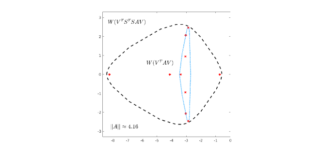
Figure 1. Example 4.2. Fields of values $\partial W(\bm{V}^{\top}\!\!\bm{A}\bm{V})$ (dotted blue line) and $\partial W(\bm{V}^{\top}\!\bm{S}^{\top}\!\bm{S}\bm{A}\bm{V})$ (dashed black line), together with the corresponding eigenvalues.

Example 4.2.

Consider the following code, building the Arnoldi basis matrix $\bm{V}$ for the given $\bm{A}$ of size $n\times n$;

n=30; rng(35);
A=-toeplitz([3,-1,-0.5,zeros(1,n-3)],[3,1,1,zeros(1,n-3)]);
b=ones(n,1);b=b/norm(b);
K=[b,A*b,A*(A*b), A*(A*(A*b)), A*(A*(A*(A*b)))];  %Krylov matrix
d=size(K,2); s=2*d;
[V,R]=qr(K,0);  %Arnoldi basis
S = 1/sqrt(s)*randn(s,n);

Note that the Arnoldi relation can be recovered as A*V(:,1:d-1) = V*H; with H=R(1:d,2:d)/R(1:d-1,1:d-1);. The sketching operator $\bm{S}$ is chosen as a random Gaussian matrix [26, 24]. Figure 1 reports the fields of values $W(\bm{V}^{\top}\!\!\bm{A}\bm{V})$ and $W(\bm{V}^{\top}\!\bm{S}^{\top}\!\bm{S}\bm{A}\bm{V})$, together with the corresponding eigenvalues. The quantity $\|\bm{A}\|$ is also reported and the distance between the two boundaries clearly reaches the magnitude of this norm.

We next deepen the analysis of the properties of the projected equations (3.4). To simplify the presentation, we consider the Lyapunov equation

$$\bm{A}\bm{X}+\bm{X}\bm{A}^{\top}=cc^{\top},$$

with $c\in\mathbb{R}^{n}$ in place of the more general setting described in (1.1). Moreover, we assume that the eigenvalues of $\bm{A}$ are simple to avoid working with invariant subspaces.

As a prerequisite for our analysis, we require the following technical lemma. A similar result was proved in [28, Section 7] using the eigenvalue decomposition of the given matrix. To deal with matrix equations, here we generalize the result to the use of the Schur decomposition, which appears to be more appropriate in this context.

Lemma 4.3.

Let $(\widehat{\bm{H}}_{d}+\widehat{h}e_{d}^{\top})^{\top}=\mathcal{Q}\mathcal{R}\mathcal{Q}^{*}$ be the Schur decomposition of (the transpose of) the given matrix. For $\eta>0$, assume that there exists an index $\bar{i}\leq d$ such that $\operatorname{dist}(\mathcal{R}_{ii},W(\widehat{\bm{H}}_{d}))$ $=\mathcal{O}(\eta^{-1})$, $i=1,\ldots\bar{i}$ for an appropriate spectral ordering in the Schur decomposition. Then it holds that $\mathcal{Q}_{1,i}=\mathcal{O}((\eta/\xi)^{d})$, for $i=1,\ldots\bar{i}$, with $\xi=\max_{j\leq\bar{i}}|1/(\widehat{\bm{H}}_{d})_{j+1,j}|$.

Proof.

Let us write $\mathcal{Q}=[q_{1},\ldots,q_{d}]$. Consider the first column in the Schur decomposition, that is $(\widehat{\bm{H}}_{d}^{\top}+e_{d}\widehat{h}^{\top})q_{1}=q_{1}\mathcal{R}_{1,1}$. Let $\bm{N}:=\widehat{\bm{H}}_{d}^{\top}$ and recall that $\bm{N}$ is lower Hessenberg. For each row $k<d$ of this eigenvalue equation we have

$$\bm{N}_{k,1:k+1}q_{1:k+1,1}=q_{k,1}\mathcal{R}_{1,1}.$$

Reordering terms, $\bm{N}_{k,k+1}q_{k+1,1}=(\bm{N}_{k,k}-\mathcal{R}_{1,1})q_{k,1}+\bm{N}_{k,1:k-1}q_{1:k-1,1}$, from which we obtain

$$q_{k+1,1}=\frac{(\bm{N}_{k,k}-\mathcal{R}_{1,1})}{\bm{N}_{k,k+1}}q_{k,1}+\frac{\bm{N}_{k,1:k-1}}{\bm{N}_{k,k+1}}q_{1:k-1,1}.$$

Taking into account the unit norm of $q_{1}$ it follows

$$|q_{k+1,1}|\leq\frac{|\bm{N}_{k,k}-\mathcal{R}_{1,1}|}{|\bm{N}_{k,k+1}|}|q_{k,1}|+\frac{\|\bm{N}_{k,1:k-1}\|}{|\bm{N}_{k,k+1}|}.$$

Hence, the entries of $q_{1}$ satisfy the relation $|q_{k+1,1}|=\mathcal{O}(\xi\eta^{-1}|q_{k,1}|)$. Normalization of $q_{1}$ yields the sought after result.

For a subsequent Schur vector $q_{i}$ with $1<i\leq\bar{i}$ we have

$$\bm{N}_{k,1:k+1}q_{1:k+1,i}=q_{k,i}\mathcal{R}_{i,i}+q_{k,1:i-1}\mathcal{R}_{1:i-1,i},$$

from which $\bm{N}_{k,k+1}q_{k+1,i}=(\bm{N}_{k,k}-\mathcal{R}_{i,i})q_{k,i}+\bm{N}_{k,1:k-1}q_{1:k-1,i}+q_{k,1:i-1}\mathcal{R}_{1:i-1,i}$ follows, so that

$$q_{k+1,i}=\frac{(\bm{N}_{k,k}-\mathcal{R}_{i,i})}{\bm{N}_{k,k+1}}q_{k,i}+\frac{\bm{N}_{k,1:k-1}}{\bm{N}_{k,k+1}}q_{1:k-1,i}+\frac{\mathcal{R}_{1:i-1,i}}{\bm{N}_{k,k+1}}q_{1:k-1,i-1}.$$

Taking once again absolute values we finally obtain

$$|q_{k+1,i}|\leq\frac{|\bm{N}_{k,k}-\mathcal{R}_{i,i}|}{|\bm{N}_{k,k+1}|}|q_{k,i}|+\frac{\|\bm{N}_{k,1:k-1}\|}{|\bm{N}_{k,k+1}|}+\frac{\|\mathcal{R}_{1:i-1,i}\|}{|\bm{N}_{k,k+1}|},$$

so that $|q_{k+1,i}|=\mathcal{O}(\xi\eta^{-1}|q_{k,i}|)$. ∎

If some of the eigenvalues of $\widehat{\bm{H}}_{d}+\widehat{h}e_{d}^{\top}$ are significantly far from the field of values of $\widehat{\bm{H}}_{d}$, the first entry of the corresponding Schur vectors will be far below machine precision, orders of magnitude smaller, especially for $d\gg 10$. Therefore, to simplify the derivation, in the following proposition we will assume that these Schur vector entries are in fact zero. Such sparsity property allows us to derive the following result on the rank structure of the solution to the Lyapunov equation.

Proposition 4.4.

Let $\widehat{\bm{H}}_{d}^{\top}+e_{d}\widehat{h}^{\top}=\mathcal{Q}R\mathcal{Q}^{*}$ be the Schur decomposition of the given matrix, with $\mathcal{Q}=[q_{1},\ldots,q_{d}]$. Under the hypotheses of Lemma 4.3 in the limit for $\eta=0$, define the partition $\mathcal{Q}=[\mathcal{Q}_{0},\mathcal{Q}_{1}]$ with $e_{1}^{\top}\mathcal{Q}_{0}=0$ and $e_{1}^{\top}\mathcal{Q}_{1}\neq 0$. Then the solution $\bm{Y}_{d}$ to

(4.2) $$(\widehat{\bm{H}}_{d}+\widehat{h}e_{d}^{\top})\bm{Y}_{d}+\bm{Y}_{d}(\widehat{\bm{H}}_{d}+\widehat{h}e_{d}^{\top})^{*}=e_{1}\beta^{2}e_{1}^{*}$$

is given by $\bm{Y}_{d}=\mathcal{Q}_{1}\mathcal{Z}\mathcal{Q}_{1}^{*}$ where $\mathcal{Z}$ solves

(4.3) $$\mathcal{Q}_{1}^{*}(\widehat{\bm{H}}_{d}+\widehat{h}e_{d}^{\top})\mathcal{Q}_{1}\mathcal{Z}+\mathcal{Z}\mathcal{Q}_{1}^{*}(\widehat{\bm{H}}_{d}+\widehat{h}e_{d}^{\top})^{*}\mathcal{Q}_{1}=\mathcal{Q}_{1}^{*}e_{1}\beta^{2}e_{1}^{*}\mathcal{Q}_{1}.$$

Proof.

Left and right multiplication of (4.2) by $\mathcal{Q}^{*}$ and $\mathcal{Q}$, respectively, gives

(4.4) $$\mathcal{Q}^{*}(\widehat{\bm{H}}_{d}+\widehat{h}e_{d}^{\top})\mathcal{Q}\mathcal{Q}^{*}\bm{Y}_{d}\mathcal{Q}+\mathcal{Q}^{*}\bm{Y}_{d}\mathcal{Q}\mathcal{Q}^{*}(\widehat{\bm{H}}_{d}+\widehat{h}e_{d}^{\top})^{*}\mathcal{Q}=\mathcal{Q}^{*}e_{1}\beta^{2}e_{1}^{*}\mathcal{Q}.$$

Using the hypotheses, $\mathcal{Q}^{*}e_{1}\beta=[0;q]$ with $q=\mathcal{Q}_{1}^{*}e_{1}\beta$. Let us use the partitions

$$\mathcal{Q}^{*}(\widehat{\bm{H}}_{d}+\widehat{h}e_{d}^{\top})\mathcal{Q}=:\!\begin{bmatrix}\mathcal{R}_{11}^{*}&0\\ \mathcal{R}_{12}^{*}&\mathcal{R}_{22}^{*}\end{bmatrix},\,\,\mathcal{Q}^{*}\bm{Y}_{d}\mathcal{Q}=:\!\begin{bmatrix}\mathcal{Z}_{11}&\mathcal{Z}_{12}\\ \mathcal{Z}_{12}^{*}&\mathcal{Z}_{22}\end{bmatrix},\,\,\mathcal{Q}^{*}e_{1}e_{1}^{*}\mathcal{Q}=:\!\begin{bmatrix}0&0\\ 0&qq^{*}\end{bmatrix}.$$

Then equating all blocks in (4.4) we obtain

(4.5) $$\mathcal{R}_{11}^{*}\mathcal{Z}_{11}+\mathcal{Z}_{11}\mathcal{R}_{11}=0,\quad\mathcal{R}_{12}^{*}\mathcal{Z}_{11}+\mathcal{R}_{22}^{*}\mathcal{Z}_{12}^{*}+\mathcal{Z}_{12}^{*}\mathcal{R}_{11}=0,$$

and

(4.6) $$\mathcal{R}_{11}^{*}\mathcal{Z}_{12}+\mathcal{Z}_{11}\mathcal{R}_{12}+\mathcal{Z}_{12}\mathcal{R}_{22}=0,\quad\mathcal{R}_{12}^{*}\mathcal{Z}_{12}+\mathcal{R}_{22}^{*}\mathcal{Z}_{22}+\mathcal{Z}_{12}^{*}\mathcal{R}_{12}+\mathcal{Z}_{22}\mathcal{R}_{22}=qq^{*}.$$

From the left matrix equation in (4.5) we obtain $\mathcal{Z}_{11}=0$, since $\mathcal{R}_{11}$ is nonsingular. This in turn leads to $\mathcal{Z}_{12}=0$ from the right equation, since $\mathcal{R}_{11}$ and $\mathcal{R}_{22}$ have distinct eigenvalues. The left matrix equation in (4.6) is then an identity. The right matrix equation in (4.6) gives the sought after solution $\mathcal{Z}=\mathcal{Z}_{22}$. ∎

In light of the previous result, for $\mathcal{Q}_{1}\in{\mathbb{C}}^{d\times\ell}$, we call the effective field of values of $\widehat{\bm{H}}_{d}+\widehat{h}e_{d}^{\top}$ the set

$$W_{\textnormal{eff}}(\widehat{\bm{H}}_{d}+\widehat{h}e_{d}^{\top})=W(\mathcal{Q}_{1}^{*}(\widehat{\bm{H}}_{d}+\widehat{h}e_{d}^{\top})\mathcal{Q}_{1})=\left\{\frac{v^{*}\mathcal{Q}_{1}^{*}(\widehat{\bm{H}}_{d}+\widehat{h}e_{d}^{\top})\mathcal{Q}_{1}v}{v^{*}v},\,\,0\neq v\in{\mathbb{C}}^{\ell}\right\}.$$

The following example illustrates the difference between the field of values and the effective field of values.

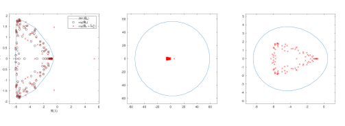
Figure 2. Example 4.5. Left: $\partial W(\bm{\widehat{H}}_{d})$ (blue solid line) spectra of $\bm{\widehat{H}}_{d}$ (black circles) and $\bm{\widehat{H}}_{d}+\widehat{h}e_{d}^{\top}$ (red crosses). Center: $\partial W(\bm{\widehat{H}}_{d}+\widehat{h}e_{d}^{\top})$ (blue solid line) and spectrum of $\bm{\widehat{H}}_{d}+\widehat{h}e_{d}^{\top}$ (red crosses). Right: $\partial W(\mathcal{Q}_{1}^{*}(\bm{\widehat{H}}_{d}+\widehat{h}e_{d}^{\top})\mathcal{Q}_{1})$ (blue solid line) and spectrum of $\mathcal{Q}_{1}^{*}(\bm{\widehat{H}}_{d}+\widehat{h}e_{d}^{\top})\mathcal{Q}_{1}$ (red crosses).

Example 4.5.

For this example we take inspiration from [28, Example 5.6]. In particular, we set $d=100$ and construct the matrix $\bm{\widehat{H}}_{d}$ and the vector $\widehat{h}$ as follows

rng(21*pi); d=100;
Hhat=toeplitz([-4, 2, zeros(1,d-2)], [-4, 1/2, 1/2, randn(1,d-3)/20]);
hhat=flipud(linspace(1,20,d))’.*randn(d,1);

In Figure 2 (left) we report $\partial W(\bm{\widehat{H}}_{d})$ (blue solid line) along with the spectra of $\bm{\widehat{H}}_{d}$ (black circles) and $\bm{\widehat{H}}_{d}+\widehat{h}e_{d}^{\top}$ (red crosses). This figure shows that, although $\bm{\widehat{H}}_{d}$ is negative definite, the matrix $\bm{\widehat{H}}_{d}+\widehat{h}e_{d}^{\top}$ has eigenvalues with positive real part. In particular, the set $W(\bm{\widehat{H}}_{d}+\widehat{h}e_{d}^{\top})$ reported in Figure 2 (center) significantly trespasses the imaginary axis. This may jeopardize the well-posedness of the projected equation (4.2) and/or the positive semidefiniteness of its solution $\bm{Y}_{d}$. This situation is mitigated by looking at the effective field of values of $\bm{\widehat{H}}_{d}+\widehat{h}e_{d}^{\top}$, namely $W(\mathcal{Q}_{1}^{*}(\bm{\widehat{H}}_{d}+\widehat{h}e_{d}^{\top})\mathcal{Q}_{1})$; see Figure 2 (right). Indeed, $W(\mathcal{Q}_{1}^{*}(\bm{\widehat{H}}_{d}+\widehat{h}e_{d}^{\top})\mathcal{Q}_{1})$ is much smaller than $W(\bm{\widehat{H}}_{d}+\widehat{h}e_{d}^{\top})$ and all the eigenvalues of $\mathcal{Q}_{1}^{*}(\bm{\widehat{H}}_{d}+\widehat{h}e_{d}^{\top})\mathcal{Q}_{1}$ have negative real part. This means that the matrix $\bm{Y}_{d}$ can be constructed by first computing the solution $\mathcal{Z}$ to (4.3) and then setting $\bm{Y}_{d}=\mathcal{Q}_{1}\mathcal{Z}\mathcal{Q}_{1}^{*}$. This guarantees both the existence and the positive semidefiniteness of $\bm{Y}_{d}$.

Remark 4.6.

Proposition 4.4 deals with the Lyapunov equation. The general Sylvester equation is more involved. The analysis comprises the sketched distortion of both coefficient matrices. While neither matrix is constrained to lie on one side of the complex plane, a vertical line separating the modified fields of values is still desirable so as to prevent instabilities. Nonetheless, the concept of effective field of values can be applied to both left and right matrices, and a result similar to Proposition 4.4 can again been obtained, possibly allowing the line constraint to still be satisfied also in case the original fields of values do not grant it.

4.2. Convergence analysis for the Lyapunov setting

We focus again on the Lyapunov equation

(4.7) $$\bm{A}\bm{X}+\bm{X}\bm{A}^{\top}=cc^{\top},$$

where, for convenience, we assume that the right-hand side has rank 1 and that $\|c\|=1$.

We next show that if $\bm{A}$ and the reduced matrix $\widehat{\bm{H}}_{d}+\widehat{h}e_{d}^{\top}$ are both negative definite, a convergence analysis is possible in a very similar way to the standard, non-sketched setting. We closely follow the techniques from [36].

Theorem 4.7.

Let $\bm{A}$ be negative definite and let $\bm{X}_{d}^{\textsc{{sk}}}$ denote the sketched-and-whitened Arnoldi approximation for the solution of (4.7). Assume that $\widehat{\bm{H}}_{d}+\widehat{h}e_{d}^{\top}$ is negative definite as well and denote $\alpha_{\max}:=\max\{\alpha(\bm{A}),\alpha(\widehat{\bm{H}}_{d}+\widehat{h}e_{d}^{\top})\}$.

Further, let $\mathbb{E}\subset\mathbb{C}^{-}$ be a compact, convex set containing the field of values of both $\bm{A}$ and $\widehat{\bm{H}}_{d}+\widehat{h}e_{d}^{\top}$, let $\Phi_{k},k=0,1,\dots$ with $\deg(\Phi_{k})=k$ denote the Faber polynomials with respect to $\mathbb{E}$ and let

(4.8) $$\exp(\tau z)=\sum\limits_{k=0}^{\infty}f_{k}(\tau)\Phi_{k}(z),$$

be the Faber series of the exponential. Then

(4.9) $$\|\bm{X}-\bm{X}_{d}^{\textsc{{sk}}}\|\leq 2\eta_{\varepsilon}\sum_{k=d}^{\infty}\int_{0}^{\infty}\exp(\tau\alpha_{\max})|f_{k}(\tau)|d\tau,$$

with $\eta_{\varepsilon}=\left(1+\sqrt{\frac{1+\varepsilon}{1-\varepsilon}}\right)\left(1+\frac{1}{\sqrt{1-\varepsilon}}\right)$.

Proof.

We have $\bm{X}_{d}^{\textsc{{sk}}}=\widehat{\bm{U}}_{d}\bm{Y}_{d}^{\textsc{sk}}\widehat{\bm{U}}_{d}^{\top}$ with

$$(\widehat{\bm{H}}_{d}+\widehat{h}e_{d}^{\top})\bm{Y}_{d}^{\textsc{sk}}+\bm{Y}_{d}^{\textsc{sk}}(\widehat{\bm{H}}_{d}+\widehat{h}e_{d}^{\top})^{\top}=e_{1}\beta^{2}e_{1}^{\top},$$

where $\beta=\|\bm{S}_{\bm{U}}c\|$. Therefore, using the standard integral representation for the solution of the Lyapunov equation,

$$\bm{X}_{d}^{\textsc{{sk}}} =\widehat{\bm{U}}_{d}\bm{Y}_{d}^{\textsc{sk}}\widehat{\bm{U}}_{d}^{\top}$$

$$=\int_{0}^{\infty}\widehat{\bm{U}}_{d}\exp(\tau(\widehat{\bm{H}}_{d}+\widehat{h}e_{d}^{\top}))e_{1}\beta^{2}e_{1}^{\top}\exp(\tau(\widehat{\bm{H}}_{d}+\widehat{t}e_{d}^{\top})^{\top})\widehat{\bm{U}}_{d}^{\top}d\tau,$$

(4.10) $$=\int_{0}^{\infty}x^{\textsc{{sk}}}(\tau)(x^{\textsc{{sk}}}(\tau))^{\top}d\tau,$$

with the short-hand notation $x^{\textsc{{sk}}}(\tau):=\widehat{\bm{U}}_{d}\exp(\tau(\widehat{\bm{H}}_{d}+\widehat{h}e_{d}^{\top}))e_{1}\beta$ for the sketched Krylov approximation of $x(\tau):=\exp(\tau\bm{A})c$.

Subtracting (4.10) from the integral representation $\bm{X}=\int_{0}^{\infty}x(\tau)(x(\tau))^{\top}d\tau$ gives

$$\|\bm{X}-\bm{X}_{d}^{\textsc{{sk}}}\| \leq\int_{0}^{\infty}\|x(\tau)(x(\tau))^{\top}-x_{d}^{\textsc{{sk}}}(\tau)(x_{d}^{\textsc{{sk}}}(\tau))^{\top}\|$$

$$\leq\int_{0}^{\infty}(\|x(\tau)\|+\|x_{d}^{\textsc{{sk}}}(\tau)\|)\|x(\tau)-x_{d}^{\textsc{{sk}}}(\tau)\|d\tau$$

(4.11) $$\leq(1+\|\widehat{\bm{U}}_{d}\|)\int_{0}^{\infty}\exp(\tau\alpha_{\max})\|x(\tau)-x^{\textsc{{sk}}}(\tau)\|d\tau,$$

where for the last inequality we have used $\|x(\tau)\|\leq\exp(\tau\alpha_{\max})$ and $\|x_{d}^{\textsc{{sk}}}(\tau)\|\leq\exp(\tau\alpha_{\max})\|\widehat{\bm{U}}_{d}\|$. To bound the norm inside the integral in (4.11), we use the Faber series (4.8) together with the polynomial exactness property

$$\widehat{\bm{U}}_{d}p_{d-1}(\widehat{\bm{H}}_{d}+\widehat{h}e_{d}^{\top})e_{1}=p_{d-1}(\bm{A})c,$$

for any polynomial of degree at most $d-1$, which gives

(4.12) $$x(\tau)-x_{d}^{\textsc{{sk}}}(\tau)=\sum_{k=d}^{\infty}f_{k}(\tau)(\Phi_{k}(\bm{A})c-\widehat{\bm{U}}_{d}\Phi_{k}(\widehat{\bm{H}}_{d}+\widehat{h}e_{d}^{\top})e_{1}\beta).$$

Taking norms in (4.12) yields

(4.13) $$\|x(\tau)-x_{d}^{\textsc{{sk}}}(\tau)\|\leq\sum_{k=d}^{\infty}|f_{k}(\tau)|(\|\Phi_{k}(\bm{A})\|+\beta\|\widehat{\bm{U}}_{d}\|\|\Phi_{k}(\widehat{\bm{H}}_{d}+\widehat{h}e_{d}^{\top})\|).$$

By [7, Théorème 1.1], we have $\|\Phi_{k}(\bm{A})\|\leq 2,\|\Phi_{k}(\widehat{\bm{H}}_{d}+\widehat{h}e_{d}^{\top})\|\leq 2$, by [5, Corollary 2.2] it holds $\|\widehat{\bm{U}}_{d}\|\leq\frac{1}{\sqrt{1-\varepsilon}}$ and further $\beta=\|\bm{S}_{\bm{U}}c\|\leq\sqrt{1+\varepsilon}\|c\|=\sqrt{1+\varepsilon}$, because $\bm{S}_{\bm{U}}$ is an $\varepsilon$-subspace embedding for $\mathcal{K}_{d+1}(\bm{A},c).$ Inserting these relations into (4.13) gives

$$\|x(\tau)-x_{d}^{\textsc{{sk}}}(\tau)\|\leq 2\left(1+\sqrt{\frac{1+\varepsilon}{1-\varepsilon}}\right)\sum_{k=d}^{\infty}|f_{k}(\tau)|.$$

Further inserting this into (4.11) and using the bound $\|\widehat{\bm{U}}_{d}\|\leq\frac{1}{\sqrt{1-\varepsilon}}$ once again completes the proof. ∎

Note that for the usually assumed sketching quality $\varepsilon=1/\sqrt{2}$, we have

$$2\eta_{\varepsilon}\approx 19.45.$$

The result of Theorem 4.7 is very similar to what one can obtain in the non-sketched setting. In that case, a bound like (4.9) holds, where the factor $2\eta_{\varepsilon}$ is replaced by $8$, one can use $\exp(\tau\alpha(\bm{A}))$ instead of $\exp(\tau\alpha_{\max})$, and $\mathbb{E}$ only needs to contain $W(\bm{A})$, as it then also contains $W(\bm{\mathscr{H}}_{d})$. This shows that as long as $W(\widehat{\bm{H}}_{d}+\widehat{h}e_{d}^{\top})$ is not much larger than $W(\bm{A})$, one can expect the sketched method to converge similarly to the non-sketched variant.

For specific shapes of the set $\mathbb{E}$, the bound in Theorem 4.7 can be made more explicit. The following corollary exemplifies this for the case that $\mathbb{E}$ is an ellipse.

Corollary 4.8.

Let the assumptions of Theorem 4.7 hold and further assume that $\mathbb{E}$ is an ellipse in $\mathbb{C}^{-}$ with center $(-c,0)$, foci $(-c,\pm\delta)$ and semi-axes $a_{1}$ and $a_{2}$, so that $\delta=\sqrt{a_{1}^{2}-a_{2}^{2}}$. Define $\rho_{1}=\frac{a_{1}+a_{2}}{2}$ and $\rho_{2}=\frac{c-\alpha_{\max}}{2\rho_{1}}+\frac{1}{2\rho_{1}}\sqrt{(c-\alpha_{\max})^{2}-\delta^{2}}$. Then

$$\|\bm{X}-\bm{X}_{d}^{\textsc{{sk}}}\|\leq 2\eta_{\varepsilon}\frac{1}{\sqrt{(c-\alpha_{\max})^{2}-\delta^{2}}}\frac{\rho_{2}}{\rho_{2}-1}\left(\frac{1}{\rho_{2}}\right)^{d}.$$

Proof.

This proof works along the same lines as that of [36, Proposition 4.1], exploiting that the Faber coefficients for $\mathbb{E}$ have an explicit representation in terms of the modified Bessel functions $I_{k}$, giving

$$\|\bm{X}-\bm{X}_{d}^{\textsc{{sk}}}\| \leq 2\eta_{\varepsilon}\sum_{k=d}^{\infty}\int_{0}^{\infty}\exp(\tau\alpha_{\max})\left(\exp(-\tau c)I_{k}(\tau\delta)\widehat{\rho}^{d}\right)d\tau,$$

with $\widehat{\rho}=\frac{2\rho_{1}}{\delta}$.

The integral above is essentially a Laplace transform of the modified Bessel function, which is explicitly known,

$$\int_{0}^{\infty}\exp(-\tau s)I_{k}(\delta\tau)d\tau=\frac{\delta^{k}}{\sqrt{\gamma^{2}-\delta^{2}}(s+\sqrt{s^{2}-\delta^{2}})^{k}}.$$

In our setting, we have $s=c-\alpha_{\max}$, so that we obtain

$$\|\bm{X}-\bm{X}_{d}^{\textsc{{sk}}}\| \leq 2\eta_{\varepsilon}\sum_{k=d}^{\infty}\widehat{\rho}^{k}\frac{\delta^{k}}{\sqrt{(c-\alpha_{\max})^{2}-\delta^{2}}(c-\alpha_{\max}+\sqrt{(c-\alpha_{\max})^{2}-\delta^{2}})^{k}}.$$

The assertion of the corollary now follows by standard algebraic manipulations. ∎

The results above may appear to be of rather limited use, since $W(\widehat{\bm{H}}_{d}+\widehat{h}e_{d}^{\top})$ may significantly differ from $W(\bm{A})$. However, the results that led us to introduce the effective field of values of $\widehat{\bm{H}}_{d}+\widehat{h}e_{d}^{\top}$ enable us to obtain more informative convergence bounds. Indeed, under the hypotheses of Proposition 4.4, we have

$$\bm{X}_{d}^{\textsc{{sk}}} = (\widehat{\bm{U}}_{d}\mathcal{Q}_{1})\mathcal{Z}(\widehat{\bm{U}}_{d}\mathcal{Q}_{1})^{*}$$

$$= \int_{0}^{\infty}\widehat{\bm{U}}_{d}\mathcal{Q}_{1}\exp(\tau(\mathcal{Q}_{1}^{*}(\widehat{\bm{H}}_{d}+\widehat{h}e_{d}^{\top})\mathcal{Q}_{1})\mathcal{Q}_{1}^{*}e_{1}\beta^{2}e_{1}^{\top}\mathcal{Q}_{1}\exp(\tau(\mathcal{Q}_{1}^{*}(\widehat{\bm{H}}_{d}+\widehat{t}e_{d}^{\top})\mathcal{Q}_{1})^{*})\mathcal{Q}_{1}^{*}\widehat{\bm{U}}_{d}^{\top}d\tau$$

$$= \int_{0}^{\infty}x^{\textsc{{sk}}}(\tau)(x^{\textsc{{sk}}}(\tau))^{\top}d\tau,$$

where

$$x^{\textsc{{sk}}}(\tau)=\widehat{\bm{U}}_{d}\exp(\tau(\widehat{\bm{H}}_{d}+\widehat{h}e_{d}^{\top}))e_{1}\beta=\widehat{\bm{U}}_{d}\mathcal{Q}_{1}\exp(\tau(\mathcal{Q}_{1}^{*}(\widehat{\bm{H}}_{d}+\widehat{h}e_{d}^{\top})\mathcal{Q}_{1}))\mathcal{Q}_{1}^{*}e_{1}\beta,$$

and the last equality follows from noticing that under the proposition hypotheses, $\mathcal{Q}^{*}e_{1}=[0;\mathcal{Q}_{1}^{*}e_{1}]$. In particular, in the proof of Theorem 4.7, we have that $\|x^{\textsc{{sk}}}(\tau)\|\leq\exp(\tau\alpha_{\max}^{\prime})$, where $\alpha_{\max}^{\prime}$ is the rightmost point of $W_{\textnormal{eff}}(\widehat{\bm{H}}_{d}+\widehat{h}e_{d}^{\top})$. Moreover,

$$\|x(\tau)-x_{d}^{\textsc{{sk}}}(\tau)\|\leq\sum_{k=d}^{\infty}|f_{k}(\tau)|(\|\Phi_{k}(\bm{A})\|+\beta\|\widehat{\bm{U}}_{d}\|\|\Phi_{k}(\mathcal{Q}_{1}^{*}(\widehat{\bm{H}}_{d}+\widehat{h}e_{d}^{\top})\mathcal{Q}_{1})\|).$$

It thus follows that we can obtain a result such as Theorem 4.7 based on the effective field of values of $\widehat{\bm{H}}_{d}+\widehat{h}e_{d}^{\top}$, which can be significantly closer to that of $\widehat{\bm{H}}_{d}$ than $W(\widehat{\bm{H}}_{d}+\widehat{h}e_{d}^{\top})$.

Corresponding convergence results can be obtained for the Sylvester equation, taking into account spectral properties of both left and right coefficient matrices, with only technical modifications. To avoid proliferation of similar results, we omit this derivation.

5. The algorithms

We report the complete algorithms presented in the previous sections for solving the Sylvester equation. In Algorithm 1 we depict the sketched-and-truncated approach for Sylvester equations. The truncated Arnoldi method for (1.1) is illustrated in Algorithm 2 in Appendix A.

Along with the definition of the projected problem and the residual norm expression, the main difference between Algorithm 2 and Algorithm 1 lies in the update of the QR factorizations of the sketched bases in 12. In particular, only the update of the QR decomposition is performed in 12 of Algorithm 1. Similarly, the new block upper Hessenberg matrix $\widehat{\bm{H}}_{d+1}=\bm{T}_{\bm{U},d+1}\bm{H}_{d+1}\bm{T}_{\bm{U},d+1}^{-1}$ is not recomputed from scratch but rather updated: if $\bm{T}_{\bm{U},d+1}$ is as in Proposition 2.1, then a direct computation shows that $\bm{T}_{\bm{U},d+1}^{-1}=\begin{bmatrix}\bm{T}_{\bm{U},d}^{-1}&\bm{T}_{\bm{U},d}^{-1}T_{H}\bm{\tau}_{d+1}^{-1}\\ &\bm{\tau}_{d+1}^{-1}\\ \end{bmatrix}$ so that

$$\small\widehat{\bm{H}}_{d+1}=\begin{bmatrix}\widehat{\bm{H}}_{d}+T_{H}\bm{h}_{d+1,d}{\bm{\tau}}_{d}^{-1}E_{d}^{\top}&\widehat{H}_{\textnormal{new}}\\ {\bm{\tau}}_{d+1}\bm{h}_{d+1,d}{\bm{\tau}}_{d}^{-1}E_{d}^{\top}&{\bm{\tau}}_{d+1}(\bm{h}_{d+1,d}{\bm{\tau}}_{d}^{-1}E_{d}^{\top}T_{H}+\bm{h}_{d+1,d+1}){\bm{\tau}}_{d+1}^{-1}\\ \end{bmatrix},$$

where $\widehat{H}_{\textnormal{new}}=(\widehat{\bm{H}}_{d}+T_{H}\bm{h}_{d+1,d}{\bm{\tau}}_{d}^{-1}E_{d}^{\top})T_{H}{\bm{\tau}}_{d+1}^{-1}+\bm{T}_{d}H{\bm{\tau}}_{d+1}^{-1}+T_{H}\bm{h}_{d+1,d+1}{\bm{\tau}}_{d}^{-1}$ and $H=[\bm{h}_{1,d+1}^{\top},\ldots,\bm{h}_{d,d+1}^{\top}]^{\top}\in\mathbb{R}^{dr\times r}$. A corresponding update for $\widehat{\bm{G}}_{d+1}$ is performed.

Algorithm 1 Sketched-and-truncated Arnoldi method for Sylvester equations

1:Input:   $\bm{A}\in\mathbb{R}^{n_{1}\times n_{1}}$, $\bm{B}\in\mathbb{R}^{n_{2}\times n_{2}}$, $C_{1}\in\mathbb{R}^{n_{1}\times r}$, $C_{2}\in\mathbb{R}^{n_{2}\times r}$, $\bm{S}_{\bm{U}}\in\mathbb{R}^{s\times n_{1}}$, $\bm{S}_{\bm{V}}\in\mathbb{R}^{s\times n_{2}}$, integers $0<k\leq\text{maxit}\ll\min\{n_{1},n_{2}\}$, $\texttt{tol}>0$, $p\geq 1$

2:Output: $\bm{X}^{(1)},\bm{X}^{(2)}$ such that $\bm{X}^{(1)}(\bm{X}^{(2)})^{\top}=\bm{X}_{d}$ approximately solves $\bm{A}\bm{X}+\bm{X}\bm{B}=C_{1}C_{2}^{\top}$

3:Compute skinny QRs: $U_{1}\bm{\ell}=C_{1}$, $V_{1}\bm{s}=C_{2}$, $\bm{Q}_{\bm{U},1}\bm{\beta}_{1}=\bm{S}_{\bm{U}}C_{1}$, $\bm{Q}_{V,1}\bm{\beta}_{2}=\bm{S}_{\bm{U}}C_{2}$, and set $\bm{T}_{\bm{U},1}=\bm{\beta}_{1}$, $\bm{T}_{V,1}=\bm{\beta}_{2}$

4:for $d=1,\ldots,\text{maxit}$ do

5:     Compute $\,\,\widetilde{U}=\bm{A}U_{d}$, $\,\,\widetilde{V}=\bm{B}^{\top}V_{d}$

6:     for $i=\max\{1,d-k+1\},\ldots,d$ do

7:         Set $\widetilde{U}=\widetilde{U}-U_{i}\bm{h}_{i,d}\,\,$ with $\,\,\bm{h}_{i,d}=U_{i}^{\top}\widetilde{U}$

8:         Set $\widetilde{V}=\widetilde{V}-V_{i}\bm{g}_{i,d}\,\,$ with $\,\,\bm{g}_{i,d}=V_{i}^{\top}\widetilde{V}$

9:     end for

10:     Compute skinny QRs: $U_{d+1}\bm{h}_{d+1,d}=\widetilde{U}$ and $V_{d+1}\bm{g}_{d+1,d}=\widetilde{V}$

11:     Update QRs: $\bm{Q}_{\bm{U},d+1}\bm{T}_{\bm{U},d+1}=\bm{S}_{\bm{U}}[\bm{U}_{d},U_{d+1}]$,

12:        $\bm{Q}_{V,d+1}\bm{T}_{V,d+1}=\bm{S}_{\bm{V}}[\bm{V}_{d},V_{d+1}]$ 

13:     Update $\widehat{\bm{H}}_{d}=\bm{T}_{\bm{U},d}\bm{H}_{d}\bm{T}_{\bm{U},d}^{-1}$, $\widehat{H}=T_{H}\bm{h}_{d+1,d}\bm{\tau_{d}}^{-1}$,

14:      $\widehat{\bm{G}}_{d}=\bm{T}_{V,d}\bm{G}_{d}\bm{T}_{V,d}^{-1}$, $\widehat{G}=T_{G}\bm{g}_{d+1,d}\bm{\theta}_{d}^{-1}$

15:     if $\mathtt{mod}(d,p)=0$ then

16:         Solve $\,\,(\widehat{\bm{H}}_{d}+\widehat{H}E_{d}^{\top})\bm{Y}+\bm{Y}(\widehat{\bm{G}}_{d}+\widehat{G}E_{d}^{\top})^{\top}=E_{1}\bm{\beta}_{1}\bm{\beta}^{\top}_{2}E_{1}^{\top}$ for $\bm{Y}$

17:         Compute $\rho=\sqrt{\|\bm{h}_{d+1,d}E_{d}^{\top}\bm{Y}\|_{F}^{2}+\|\bm{Y}E_{d}\bm{g}_{d+1,d}^{\top}\|_{F}^{2}}$ 

18:         if $\rho<\texttt{tol}$ then

19:              Go to line 23

20:         end if

21:     end if

22:end for

23:Compute (possibly low-rank) factors $\bm{Y}_{1},\bm{Y}_{2}$ such that $\bm{Y}\approx\bm{Y}_{1}\bm{Y}_{2}^{\top}$

24:Retrieve $\bm{X}^{(1)}=\bm{U}_{d}\bm{T}_{\bm{U},d}^{-1}\bm{Y}_{1}$, $\bm{X}^{(2)}=\bm{V}_{d}\bm{T}_{V,d}^{-1}\bm{Y}_{2}$ by the two-pass step

At convergence, the matrix $\bm{T}_{\bm{U},d}^{-1}\bm{Y}_{d}(\bm{T}_{V,d}^{-1})^{\top}$ is approximated by a low-rank factorization, $\bm{T}_{\bm{U},d}^{-1}\bm{Y}_{d}(\bm{T}_{V,d}^{-1})^{\top}\approx\bm{Z}^{(1)}(\bm{Z}^{(2)})^{\top}$, with $\bm{Z}^{(1)},\bm{Z}^{(2)}\in\mathbb{R}^{dr\times\ell}$, $\ell\leq dr$ so that the final approximate solution $\bm{X}_{d}$ is available as the low-rank product $\bm{X}_{d}\approx\bm{X}^{(1)}(\bm{X}^{(2)})^{\top}=(\widehat{\bm{U}}_{d}\bm{Z}^{(1)})(\widehat{\bm{V}}_{d}\bm{Z}^{(2)})^{\top}$; cf. 23 to 24 of Algorithm 1. Since $\widehat{\bm{U}}_{d},\widehat{\bm{V}}_{d}$ are not stored, to finalize the computation a two-pass strategy is employed; see, e.g. [22, 30, 15]. More precisely, the original Arnoldi iteration is performed once again to iteratively construct the two matrices $\widehat{\bm{U}}_{d}\bm{Z}^{(1)},\widehat{\bm{V}}_{d}\bm{Z}^{(2)}$. Since the orthogonalization coefficients are available in the matrices $\bm{H}_{d},\bm{G}_{d}$, the cost of this second Arnoldi iteration does not involve inner products for the local orthogonalization. To improve efficiency, the reconstruction of $\widehat{\bm{U}}_{d}\bm{Z}^{(1)}$ and $\widehat{\bm{V}}_{d}\bm{Z}^{(2)}$ should be performed in chunks of $kr$ basis vectors at a time.

Table 1 summarizes the main memory requirements of full Arnoldi and the proposed methods. Algorithm 1 and Algorithm 2 require the same amount of long vector allocations for fixed truncation parameter $k$ and number of iterations and we thus report only the storage demand of the former.

	Memory Allocation		Memory Allocation		Extra
Method	Bases		Approximate Solution		Terms
Full Arnoldi	$\bm{\mathscr{U}}_{d},\bm{\mathscr{V}}_{d}$	$2(d+1)r\cdot n$	$(\bm{X}_{d}^{\textsc{full}})^{(1)},(\bm{X}_{d}^{\textsc{full}})^{(2)}$	$2\ell\cdot n$	${\mathcal{O}}(d^{2}r^{2})$
Algorithm 1	$\widehat{\bm{U}}_{d},\widehat{\bm{V}}_{d}$	$2(k+1)r\cdot n$	$\bm{X}^{(1)},\bm{X}^{(2)}$	$2\ell\cdot n$	${\mathcal{O}}(d^{2}r^{2}+drs)$

Table 1. Memory requirements of full Arnoldi and Algorithm 1.

For $k,\ell\ll d$ the main difference between the two classes of methods stands in the memory allocations for the generated bases. On the other hand, storage for the solution factors depends on the spectral decay properties of the solution to the reduced problem. Since the polynomial Krylov space generates redundant information, the numerical rank $\ell$ of $\bm{Y}_{d}$ may be significantly lower than its dimension, allowing major savings in storing the approximate solution in factored form. We refer to the examples of Section 6 for experimental evidence. The extra allocations concern matrices in the reduced spaces, together with the $s\times dr$ sketched basis, which is kept orthonormal.

Finally, we remark that our stopping criterion is based on the residual norm or its estimation, in both algorithms. This criterion is checked periodically, not necessarily at each iteration, to save computational efforts.

6. Numerical experiments

In this section we report numerical experiments to illustrate the potential of the new algorithms. In all the experiments presented here, we employ the sketching matrix $\bm{S}=\sqrt{s/n}\cdot\bm{DNE}\in\mathbb{R}^{s\times n}$ where $\bm{E}\in\mathbb{R}^{n\times n}$ is a diagonal matrix containing Rademacher random variables on its diagonal, $\bm{N}\in\mathbb{R}^{n\times n}$ denotes the discrete cosine transform matrix and $\bm{D}\in\mathbb{R}^{s\times n}$ randomly selects $s$ rows.

All the experiments have been run using Matlab (version 2022b) on a machine with a 1.2GHz Intel quad-core i7 processor with 16GB RAM on an Ubuntu 20.04.2 LTS operating system.

Example 6.1.

We compare the new sketched-and-truncated method with the full Arnoldi method. Moreover, we analyze the role of the truncation parameter in the performance of the new algorithm.

We consider the matrices $\bm{A}$ and $\bm{B}$ in (1.1) coming from the discretization of a convection-diffusion differential operator of the form

(6.1) $$\mathcal{L}(u)=-\nu\Delta u+w\nabla u,$$

on the unit square $[0,1]^{2}$ by centered finite differences using 300 nodes in each direction, yielding $\bm{A},\bm{B}\in\mathbb{R}^{n\times n}$, $n=90\,000$. We consider the same viscosity parameter $\nu$ in the construction of both $\bm{A}$ and $\bm{B}$ whereas for the convection vectors we use $w_{\bm{A}}=(1,1)$ for $\bm{A}$ and $w_{\bm{B}}=(3y(1-x^{2}),-2x(1-y^{2}))$ for $\bm{B}$. The vectors $c_{1},c_{2}\in\mathbb{R}^{n}$ in (1.1) have random entries drawn from the standard normal distribution and are normalized to have unit norm. The threshold for the stopping criterion in Algorithm 1 and Algorithm 2 is $\texttt{tol}=10^{-6}$.

We start by comparing the full Arnoldi method and Algorithm 1. In both procedures we solve the projected equation, and thus check the stopping criterion, every $p$ iterations with $p\in\{1,10\}$. The truncation parameter in Algorithm 1 is set to $k=10$, the sketching dimension is $s=1\,200$ and maxit$=600$.

	Full Arnoldi						Algorithm 1
	$p=1$			$p=10$			$p=1$			$p=10$
$\nu$	$d$	Time	Mem	$d$	Time	Mem	$d$	Time	Mem	$d$	Time	Mem
$0.1$	460	117.69	922	460	90.49	922	452	44.10	74	460	14.95	74
$0.01$	553	185.65	1 108	560	133.50	1 122	550	77.80	104	550	20.05	104
$0.001$	745	409.26	1 492	750	255.58	1 502	766	217.30	194	770	43.99	194

Table 2. Example 6.1. Performance of the full Arnoldi method and Algorithm 1. The reported CPU timings are in seconds. “Mem” indicates the number of vectors of length $n$ used.

In Table 2 we report the number of iterations and CPU times of the full Arnoldi method and the sketched-and-truncated scheme, as $\nu$ varies. The two schemes perform a very similar number of iterations for all tested values of $\nu$. This shows that on this example the basis truncation does not significantly affect (delay) convergence and the implicit use of the $\bm{S}^{\top}\!\bm{S}$-orthogonal bases $\bm{\widehat{U}}_{d}$ and $\bm{\widehat{V}}_{d}$ pays off. We recall that in Algorithm 1 we check the $\bm{S}^{\top}\!\bm{S}$-norm of the residual matrix whereas full Arnoldi computes its Frobenius norm. Although rather close thanks to the $\varepsilon$-embedding property of the sketching, these two norms may slightly differ (cf. (3.7)), leading to a small gap in the number of iterations needed to achieve a prescribed level of accuracy in the two algorithms.

Thanks to an effective truncation strategy with $k=10$, Algorithm 1 always requires less CPU time than full Arnoldi, for a similar number of iterations. Moreover, the rather small dimension of the sketching ($s=1\,200$), limits the impact of the full orthogonalization of the sketched bases on the overall solution process. We also stress that only about $k=10$ long vector allocations are required by the truncated approach for each space, as opposed to the full basis. For more on-point insight on the memory requirements, Table 2 (column labeled “Mem”) includes the number of vectors of length $n$ stored by the two algorithms. With an eye to Table 1, for full Arnoldi memory allocations are mainly due to the bases, whereas for Algorithm 1 they are mainly due to storing the low-rank factors of the computed solution for Algorithm 1. The memory requirements of Algorithm 1 are always one order of magnitude smaller than what is needed by full Arnoldi, making the sketched-and-truncated Krylov subspace method very competitive.

The cost of solving the projected equations becomes more and more dominant as the dimensions of the reduced matrices increase, being of the order of $d^{3}$. To mitigate this shortcoming and leverage the cheap basis construction of polynomial Krylov subspaces for sparse coefficient matrices, it is common practice to solve the projected problem every $p\geq 1$ iterations. Adopting this practice is much more convenient (60% savings) for Algorithm 1 than for full Arnoldi (see Table 2 for $p=10$). This is because in the latter, the cost of constructing a fully orthonormal basis still remains largely dominant.

We next turn our attention to the plain truncated scheme to analyze how different selections of the truncation parameters for the two spaces, namely $k_{\bm{A}}$ and $k_{\bm{B}}$, may affect performance. In contrast to what happens for Algorithm 1 (cf. Table 2 for $k_{\bm{B}}=10$), Algorithm 2 was unable to achieve the prescribed level of accuracy for $k_{\bm{A}}=k_{\bm{B}}=10$ within maxit=1000 iterations for any considered value of $\nu$. We thus fix $k_{\bm{A}}=40$ and in Table 3 we report the number of iterations and computational timings of Algorithm 2 when varying $\nu$ and $k_{\bm{B}}$.

	Full Arnoldi						Algorithm 2
	$p=1$			$p=10$				$p=1$			$p=10$
$\nu$	$d$	Time	Mem	$d$	Time	Mem	$k_{\bm{B}}$	$d$	Time	Mem	$d$	Time	Mem
0.1	460	117.69	922	460	90.49	922	40	587	101.99	143	590	46.04	143
							60	619	127.03	166	630	62.77	166
0.01	553	185.65	1 108	560	133.50	1 122	40	675	150.58	194	680	56.27	194
							60	744	211.61	200	750	80.74	200

Table 3. Example 6.1. Performance of the full Arnoldi method and Algorithm 2. In Algorithm 2, basis truncation parameters $k_{\bm{A}}=40$ (left space) and varying $k_{\bm{B}}$ (right space). The reported CPU timings are in seconds. “Mem” indicates the number of vectors of length $n$ used.

With these values of $k_{\bm{A}}$ and $k_{\bm{B}}$, Algorithm 2 converges and considerations about the use of $p\geq 1$ similar to the ones discussed for the sketched-and-truncated procedure still hold. Similarly for the memory requirements.

To conclude this example, we would like to highlight a somehow unexpected phenomenon: Algorithm 2 performs more iterations for $k_{\bm{B}}=60$ than for $k_{\bm{B}}=40$, in spite of the former having more orthogonal basis vectors. This peculiar aspect shows that selecting sensible values of $k$ for Algorithm 2 may be a rather difficult task. Further analysis is needed to fully understand this behavior.

Example 6.2.

For this example we take inspiration from [18, Example 5.1]. We consider the heat equation $u_{t}+\Delta u=f$ in the cube $(-1,1)^{3}$ and time interval $[0,1]$, with homogeneous Dirichlet boundary conditions and zero initial value. The source term is $f(t,x,y,z):=10\,t\sin(t)\cos(2\pi x)\cos(2\pi y)\cos(2\pi z)$ so that its space-time discretized form has rank equal to one. The discretization of this differential problem leads to the following Sylvester equation

(6.2) $$\bm{K}\bm{X}\bm{B}_{1}+\bm{M}\bm{X}\bm{B}_{2}=c_{1}c_{2}^{\top},$$

where $\bm{B}_{1}$, $\bm{B}_{2}\in\mathbb{R}^{\ell\times\ell}$, with $\ell$ the number of time steps, are such that

$$\bm{B}_{1}=\frac{1}{2(\ell-1)}\begin{bmatrix}1&&&\\ 1&1&&\\ &\ddots&\ddots&\\ &&1&1\\ \end{bmatrix},\quad\bm{B}_{2}=\begin{bmatrix}1&&&\\ -1&1&&\\ &\ddots&\ddots&\\ &&-1&1\\ \end{bmatrix},$$

and correspond to the discrete Crank-Nicolson time integrator, whereas $\bm{K}$, $\bm{M}\in\mathbb{R}^{n\times n}$ are, respectively, the stiffness and mass matrix coming from the discretization of the space component of the differential operator by linear finite elements; see [18] for more details.

We recast equation (6.2) in terms of a standard Sylvester equation by inverting $\bm{M}$ and $\bm{B}_{1}$. In particular, we consider the Sylvester equation

(6.3) $$\bm{M}^{-1}\bm{K}\bm{X}+\bm{X}\bm{B}_{2}\bm{B}_{1}^{-1}=\bm{M}^{-1}c_{1}c_{2}^{\top}\bm{B}_{1}^{-1}.$$

Thanks to the moderate number of time steps $\ell$ we consider ($\ell=800$) and the sparsity pattern of $\bm{B}_{1}$, we can explicitly construct the matrix $\bm{B}_{2}\bm{B}_{1}^{-1}$. On the other hand, the mass matrix $\bm{M}$ inherits the possibly involved sparsity pattern of $\bm{K}$. Moreover, we employ large values of degrees of freedom $n$ in space so that $\bm{M}^{-1}\bm{K}$ cannot be explicitly computed. The action of this matrix is computed on the fly during the construction of the Krylov subspace $\mathcal{K}_{d}(\bm{M}^{-1}\bm{K},\bm{M}^{-1}c_{1})$. In particular, quantities of the form $\bm{M}^{-1}v$ are approximated by applying the preconditioned conjugate gradient method (PCG) [19] with diagonal (Jacobi) preconditioning. PCG is stopped as soon as the relative residual norm is smaller than $10^{-6}$.

Following [18], equation (6.3) can be solved by performing only a left projection, that is, only the left space $\mathcal{K}_{d}(\bm{M}^{-1}\bm{K},\bm{M}^{-1}c_{1})$ is constructed. The projected problem has the form

$$\bm{\widetilde{H}}_{d}\bm{Y}+\bm{Y}\bm{B}_{2}\bm{B}_{1}^{-1}=e_{1}\bm{\beta}_{1}c_{2}^{\top}\bm{B}_{1}^{-1},$$

where $\bm{\widetilde{H}}_{d}\in\mathbb{R}^{d\times d}$ stems from the adopted projection technique, namely full Arnoldi ($\bm{\widetilde{H}}_{d}=\bm{\mathscr{H}}_{d}$), Algorithm 2 ($\bm{\widetilde{H}}_{d}=\bm{H}_{d}$), and Algorithm 1 ($\bm{\widetilde{H}}_{d}=\bm{\widehat{H}}_{d}+\widehat{H}e_{d}^{\top}$).

	Full Arnoldi			Algorithm 2			Algorithm 1
$n$	$d$	Time	Mem	$d$	Time	Mem	$d$	Time	Mem
$393968$	260	100.93	261	520	172.96	25	260	84.57	20
$482768$	280	145.43	281	780	317.47	26	320	131.25	21
$685214$	300	224.10	301	660	352.41	25	300	196.65	20
$880370$	320	327.02	321	780	531.06	26	340	258.65	20

Table 4. Example 6.2. Performance of all considered methods for varying $n$ ($\ell=800$, truncation $k=3$). The reported CPU timings are in seconds. “Mem” indicates the number of vectors of length $n$ used.

We compare the three schemes as $n$ varies, in terms of number of iterations and computational time, by checking the stopping criterion every $p=20$ iterations, and $\mathtt{tol}=10^{-6}$. For the sketched-and-truncated scheme we adopt $s=1200$; the truncation parameter takes the value $k=3$ in both Algorithm 1 and Algorithm 2.

The results displayed in Table 4 show that full Arnoldi and Algorithm 1 perform a rather similar number of iterations for all tested values of $n$ with Algorithm 1 being always faster than full Arnoldi. On the contrary, Algorithm 2 needs a much larger number of iterations to converge, at least twice as many as with Algorithm 1, leading to correspondingly large CPU time.

For this problem, the real potential of Algorithm 1 and Algorithm 2 can be appreciated by looking at their memory consumption. Indeed, both schemes require storing one order of magnitude fewer vectors of length $n$ than what is done in full Arnoldi, making the memory requirements of the former solvers extremely affordable.

Example 6.3.

In this example we compare the sketched-and-truncated strategy with the rational Krylov subspace method (RKSM); see, e.g. [13]. We consider the matrices $\bm{A},\bm{B}\in\mathbb{R}^{n\times n}$ in (1.1) coming from the centered finite differences discretization of three-dimensional convection-diffusion operators of the form (6.1) on $[0,1]^{3}$ with $\nu=0.005$ and convection vectors $w_{\bm{A}}=(x\sin(x),y\cos(y),e^{z^{2}-1})$ and $w_{\bm{B}}=((1-x^{2})yz,1,e^{z})$. The vectors $c_{1},c_{2}\in\mathbb{R}^{n}$ have normally distributed random entries, and they are such that $c_{1}c_{2}^{\top}$ has unit norm.

The shifts employed in RKSM are computed by following the on-line procedure presented in [13]. Moreover, the large shifted linear systems occurring in the basis construction are solved by means of preconditioned BICGstab($\ell$) [40] with no fill-in ILU preconditioning, and similarly for $\bm{B}$. BICGstab($\ell$) is stopped as soon as the relative residual norm reached $10^{-8}$.

The stopping threshold in Algorithm 1 and RKSM is $\texttt{tol}=10^{-6}$ while maxit$=250$. Finally, in Algorithm 1 the truncation parameter was $k=3$ while the sketching dimension was $s=500$.

	Algorithm 1				RKSM
$n$	$d$	Time	rank	Mem	$d$ ($d_{\textnormal{inn}}^{\bm{A}}$, $d_{\textnormal{inn}}^{\bm{B}}$)	Time	rank	Mem
$125\,000$	133	3.97	30	66	29 (7.9, 7.0)	9.86	28	58+36
$216\,000$	149	6.32	31	68	28 (7.6, 7.0)	17.57	27	56+36
$343\,000$	163	11.29	31	68	29 (7.9, 7.3)	30.83	27	58+36
$512\,000$	179	21.42	32	70	30 (8.3, 7.7)	48.92	28	60+36
$729\,000$	194	35.42	32	70	29 (9.2, 8.3)	76.60	28	58+36
$1\,000\,000$	210	52.56	33	72	30 (9.9, 8.6)	114.91	29	60+36

Table 5. Example 6.3. Performance of Algorithm 1 and RKSM. The reported CPU timings are in seconds. The column “rank” indicates the rank of the solution matrix $\bm{X}_{d}$ and “Mem” indicates the number of vectors of length $n$ used. For RKSM, the memory requirements are reported as the sum of the memory required for basis allocation and for the preconditioner.

In Table 5 we report the number of iterations, the computational timings and the rank of the solution computed by Algorithm 1 and RKSM by varying the problem dimension $n$. Table 5 also reports the average number of (inner) BICGStab($\ell$) iterations, $d_{\text{inn}}^{\bm{A}}$ and $d_{\text{inn}}^{\bm{B}}$, to approximately solve the shifted linear systems with $\bm{A}$ and $\bm{B}^{\top}$, respectively, during the generation of the rational Krylov spaces. Although RKSM requires a much smaller space to converge, Algorithm 1 is always faster. Indeed, the solution of two shifted linear systems (one with $\bm{A}$ and one with $\bm{B}^{\top}$) at each RKSM iteration has a detrimental impact on the overall running time. Even though these values remain rather moderate, the BICGStab($\ell$) iteration count increases with $n$, making the linear system solution step increasingly more expensive. Such shortcoming may be fixed by employing more robust preconditioning operators. On the other hand, Algorithm 1 requires only matrix-vector products and the cost of the orthogonalization step is moderate thanks to the truncated approach. Moreover, the possible delay coming from the use of locally orthogonal bases is mitigated by sketching.

Algorithm 1 turns out to be surprisingly competitive when compared to RKSM also in terms of storage allocation. Indeed, as reported in the columns “Mem” of Table 5, the memory requirements of Algorithm 1 and RKSM are always rather similar. We mention that in case of RKSM we denote the storage demand as the sum of two terms to emphasize the different nature of the allocated components. While the first one is related to the basis storage, the second one comes from the allocation of the preconditioners. Indeed, for this example, storing the four incomplete LU factors is equivalent to storing about 36 vectors of length $n$.

7. Conclusions

By fully exploiting the promising combination of sketching and Krylov methods, in this paper we developed a sketched-and-truncated Krylov subspace method for matrix equations. In addition to making polynomial Krylov methods feasible, the approach turns out to be competitive also with respect to state-of-the-art schemes based on rational Krylov subspaces. In particular, the proposed method reduces the storage demand of the overall solution process, and concurrently provides a 50% CPU time speed-up over RKSM. Therefore, the sketched-and-truncated polynomial Krylov subspace method can be a valid candidate for solving large-scale matrix equations for which projection methods based on more sophisticated subspaces struggle due to, e.g., expensive linear systems solves.

The whitened-sketched recurrence produces matrices that can, in theory, endanger the applicability of the generated space as projection method; fortunately, the projected linear equations are usually solvable in practice, and very effective performance resulted in our numerical experiments. We have theoretically explained this perceivable contradiction. Indeed, we have proved that sketching takes place into what we have called the effective field of values of the involved matrices, for which the projected solution can be well-defined.

A convergence analysis for the sketched approximation has also been presented, which conveniently extends results obtained in the literature for the full Arnoldi method.

As a supplementary numerical contribution of this paper, we have derived and analyzed truncated Krylov methods, which appear to be new in the matrix equation context.

Appendix A Algorithmic description of truncated Arnoldi

Algorithm 2 Truncated Arnoldi method for Sylvester equations

1:Input:   $\bm{A}\in\mathbb{R}^{n_{1}\times n_{1}}$, $\bm{B}\in\mathbb{R}^{n_{2}\times n_{2}}$, $C_{1}\in\mathbb{R}^{n_{1}\times r}$, $C_{2}\in\mathbb{R}^{n_{2}\times r}$, integers $0<k\leq\text{maxit}\ll\min\{n_{1},n_{2}\}$, $\texttt{tol}>0$, $p\geq 1$

2:Output: $\bm{X}^{(1)},\bm{X}^{(2)}$ such that $\bm{X}^{(1)}(\bm{X}^{(2)})^{\top}=\bm{X}_{d}$ approximately solves $\bm{A}\bm{X}+\bm{X}\bm{B}=C_{1}C_{2}^{\top}$

3:Compute skinny QRs: $U_{1}\bm{\beta}_{1}=C_{1}$, $V_{1}\bm{\beta}_{2}=C_{2}$

4:for $d=1,\ldots,maxit$ do

5:     Compute $\,\,\widetilde{U}=\bm{A}U_{d}$, $\,\,\widetilde{V}=\bm{B}^{\top}V_{d}$

6:     for $i=\max\{1,d-k+1\},\ldots,d$ do

7:         Set $\widetilde{U}=\widetilde{U}-U_{i}\bm{h}_{i,d}\,\,$ with $\,\,\bm{h}_{i,d}=U_{i}^{\top}\widetilde{U}$

8:         Set $\widetilde{V}=\widetilde{V}-V_{i}\bm{g}_{i,d}\,\,$ with $\,\,\bm{g}_{i,d}=V_{i}^{\top}\widetilde{V}$

9:     end for

10:     Compute skinny QRs: $U_{d+1}\bm{h}_{d+1,d}=\widetilde{U}$ and $V_{d+1}\bm{g}_{d+1,d}=\widetilde{V}$

11:     if $\mathtt{mod}(d,p)=0$ then

12:         Solve $\,\,\bm{H}_{d}\bm{Y}+\bm{Y}\bm{G}_{d}^{\top}=e_{1}\bm{\beta_{1}}\bm{\beta_{2}}e_{1}^{\top}$ for $\bm{Y}$

13:         Compute $\rho=\sqrt{dr}(\|\bm{Y}_{d}E_{d}\bm{g}_{d+1,d}^{\top}\|_{F}+\|\bm{h}_{d+1,d}E_{d}^{\top}\bm{Y}_{d}\|_{F})$ 

14:         if $\rho<\texttt{tol}$ then

15:              Go to line 19

16:         end if

17:     end if

18:end for

19:Compute (possibly low-rank) factors $\bm{Y}_{1},\bm{Y}_{2}$ such that $\bm{Y}\approx\bm{Y}_{1}\bm{Y}_{2}^{\top}$

20:Retrieve $\bm{X}^{(1)}=\bm{U}_{d}\bm{Y}_{1}$, $\bm{X}^{(1)}=\bm{V}_{d}\bm{Y}_{2}$ by the two-pass step

In Algorithm 2 we report the algorithm pseudocode for the truncated polynomial Krylov method for Sylvester equations. Notice that, in principle, one can use the sketched inner product also in the computation of the truncated bases $\bm{U}_{d}$ and $\bm{V}_{d}$, thus avoiding any inner product in $\mathbb{R}^{n}$. We refrain from reporting also this pseudocode here as it can be easily derived from Algorithm 2.

Appendix B Tensorized subspace embeddings

In our context of solving matrix equations, sketchings of the form $\bm{S}_{\bm{U}}\bm{M}\bm{S}_{\bm{V}}^{\top}$ occur; see, e.g., formula (3.6) involving the norm of the sketched residual.

The embeddings $\bm{S}_{\bm{U}}$ and $\bm{S}_{\bm{V}}$ are constructed as usual subspace embeddings for the block Krylov spaces $\mathcal{K}_{d+1}(\bm{A},C_{1}),\mathcal{K}_{d+1}(\bm{B}^{\top},C_{2})$, so that (2.2) holds for $\bm{S}_{\bm{U}}$ and $v\in\mathcal{K}_{d+1}(\bm{A},C_{1})$ as well as for $\bm{S}_{\bm{V}}$ and $v\in\mathcal{K}_{d+1}(\bm{B}^{\top},C_{2})$. We now investigate what this implies for $\|\bm{S}_{\bm{U}}\bm{M}\bm{S}_{\bm{V}}^{\top}\|_{F}$ in relation to $\|\bm{M}\|_{F}$, when $\bm{M}$ is of the form $\bm{M}=\bm{\mathscr{U}}_{d+1}\bm{\mathscr{Z}}\bm{\mathscr{V}}_{d+1}^{\top}$ (as it is the case for the Sylvester equation residual).

Our derivations closely follow the ideas in [10], generalizing their results from random Gaussian matrices to general $\varepsilon$-subspace embeddings. We start with the following simple observation.

Proposition B.1.

Let $\bm{S}\in\mathbb{R}^{s\times n}$ be an $\varepsilon$-subspace embedding of $\mathcal{V}$ with $\dim(\mathcal{V})=d+1$ and let the columns of $\bm{\mathscr{V}}$ form an orthonormal basis of $\mathcal{V}$. Then $\bm{S}\bm{\mathscr{V}}$ is an $\varepsilon$-subspace embedding for $\mathbb{R}^{d+1}$.

Proof.

Let $z\in\mathbb{R}^{d+1}$. Then $\bm{\mathscr{V}}z\in\mathcal{V}$, so that by (2.2), we have

$$(1-\varepsilon)\|\bm{\mathscr{V}}z\|^{2}\leq\|\bm{S}\bm{\mathscr{V}}z\|^{2}\leq(1+\varepsilon)\|\bm{\mathscr{V}}z\|^{2},$$

The result follows by noting that $\|\bm{\mathscr{V}}z\|=\|z\|$ due to the orthonormality of the columns of $\bm{\mathscr{V}}$. ∎

We further need the following auxiliary result.

Proposition B.2 (Lemma 1 and Corollary 3 in [10]).

Let $\bm{S}_{1},\bm{S}_{2}\in\mathbb{R}^{s\times(d+1)}$ be $\varepsilon$-subspace embeddings of $\mathbb{R}^{d+1}$. Then $\bm{S}_{i}\otimes\bm{I}_{n}$ and $\bm{I}_{n}\otimes\bm{S}_{i},i=1,2$ are $\varepsilon$-subspace embeddings of $\mathbb{R}^{n(d+1)}$ and $\bm{S}_{1}\otimes\bm{S}_{2}$ is an $\varepsilon(2+\varepsilon)$-subspace embedding of $\mathbb{R}^{(d+1)^{2}}$.

With these results, we can now state a tensorized embedding property.

Theorem B.3.

Let $\bm{S}_{\bm{U}}\in\mathbb{R}^{s\times n_{1}}$ be an $\varepsilon$-subspace embedding for the subspace $\mathcal{U}\subseteq\mathbb{R}^{n_{1}}$ and $\bm{S}_{\bm{V}}\in\mathbb{R}^{s\times n_{2}}$ be an $\varepsilon$-subspace embedding for the subspace $\mathcal{V}\subseteq\mathbb{R}^{n_{2}}$, with $\dim(\mathcal{U})=\dim(\mathcal{V})=d+1$. Further, let the columns of $\bm{\mathscr{U}},\bm{\mathscr{V}}$ contain orthonormal bases of $\mathcal{U},\mathcal{V}$, respectively.

Then, for any $\bm{M}=\bm{\mathscr{U}}\bm{\mathscr{Z}}\bm{\mathscr{V}}^{\top}$, we have

(B.1) $$(1-\widetilde{\varepsilon})\|\bm{M}\|_{F}\leq\|\bm{S}_{\bm{U}}\bm{M}\bm{S}_{\bm{V}}^{\top}\|_{F}\leq(1+\widetilde{\varepsilon})\|\bm{M}\|_{F}$$

with $\widetilde{\varepsilon}=\varepsilon(2+\varepsilon)$.

Proof.

Using the vectorized form, for any $\bm{M}$, we have $\|\bm{M}\|_{F}=\|\operatorname{vec}(\bm{M})\|$. By a direct calculation, we obtain

$$\|\bm{S}_{\bm{U}}\bm{M}\bm{S}_{\bm{V}}^{\top}\|_{F}=\|(\bm{S}_{\bm{V}}\bm{\mathscr{V}}\otimes\bm{S}_{\bm{U}}\bm{\mathscr{U}})\operatorname{vec}(\bm{\mathscr{Z}})\|.$$

By Proposition B.1, $\bm{S}_{\bm{U}}\bm{\mathscr{U}}$ and $\bm{S}_{\bm{V}}\bm{\mathscr{V}}$ are $\varepsilon$-subspace embeddings of $\mathbb{R}^{d+1}$, so that by Proposition B.2, $\bm{S}_{\bm{V}}\bm{\mathscr{V}}\otimes\bm{S}_{\bm{U}}\bm{\mathscr{U}}$, is an $\widetilde{\varepsilon}$-subspace embedding of $\mathbb{R}^{(d+1)^{2}}$. Thus,

(B.2) $$(1-\widetilde{\varepsilon})\|\operatorname{vec}(\bm{\mathscr{Z}})\|\leq\|(\bm{S}_{\bm{V}}\bm{\mathscr{V}}\otimes\bm{S}_{\bm{U}}\bm{\mathscr{U}})\operatorname{vec}(\bm{\mathscr{Z}})\|\leq(1+\widetilde{\varepsilon})\|\operatorname{vec}(\bm{\mathscr{Z}})\|.$$

Furthermore, $\|\operatorname{vec}(\bm{\mathscr{Z}})\|=\|\operatorname{vec}(\bm{M})\|$, because $(\bm{\mathscr{V}}\otimes\bm{\mathscr{U}})\operatorname{vec}(\bm{\mathscr{Z}})=\operatorname{vec}(\bm{M})$ and $\bm{\mathscr{V}}\otimes\bm{\mathscr{U}}$ has orthonormal columns. Inserting this into (B.2) completes the proof. ∎

Remark B.4.

The lower bound in (B.1) is only informative if $1-\widetilde{\varepsilon}>0$, or equivalently, $\varepsilon<\sqrt{2}-1\approx 0.4142$. This means that in order to obtain theoretical guarantees, one needs to impose a stricter subspace embedding condition than when solving linear systems or approximating the action of matrix functions via sketched Krylov methods (where any $\varepsilon<1$ works in principle, and $\varepsilon=1/\sqrt{2}$ guarantees that, e.g., the sketched residual norm differs from the true residual norm by a factor of at most $6$).

However, our numerical experiments indicate that in practice, a cruder tolerance typically also suffices for obtaining a method that works well.

References

- [1] A. C. Antoulas, Approximation of Large-Scale Dynamical Systems, Society for Industrial and Applied Mathematics, 2005.
- [2] W. E. Arnoldi, The principle of minimized iteration in the solution of the matrix eigenvalue problem, Q. Appl. Math. 9 (1951), 17–29.
- [3] J. Baker, M. Embree, and J. Sabino, Fast singular value decay for Lyapunov solutions with nonnormal coefficients, SIAM J. Matrix Anal. Appl. 36 (2015), no. 2, 656–668.
- [4] O. Balabanov and L. Grigori, Randomized block Gram–Schmidt process for solution of linear systems and eigenvalue problems, arXiv preprint arXiv:2111.14641 (2021).
- [5] by same author, Randomized Gram–Schmidt process with application to GMRES, SIAM J. Sci. Comput. 44 (2022), no. 3, A1450–A1474.
- [6] O. Balabanov and A. Nouy, Randomized linear algebra for model reduction. Part I: Galerkin methods and error estimation, Adv. Comput. Math. 45 (2019), no. 5, 2969–3019.
- [7] B. Beckermann, Image numérique, GMRES et polynômes de Faber, Comptes Rendus Math. 340 (2005), no. 11, 855–860.
- [8] D. A. Bini, B. Iannazzo, and B. Meini, Numerical Solution of Algebraic Riccati Equations, Society for Industrial and Applied Mathematics, 2011.
- [9] L. Burke and S. Güttel, Krylov subspace recycling with randomized sketching for matrix functions, arXiv preprint arXiv:2308.02290 (2023).
- [10] K. Chen, Q. Li, K. Newton, and S. J. Wright, Structured random sketching for PDE inverse problems, SIAM J. Matrix Anal. Appl. 41 (2020), no. 4, 1742–1770.
- [11] A. Cortinovis, D. Kressner, and Y. Nakatsukasa, Speeding up Krylov subspace methods for computing via randomization, arXiv preprint arXiv:2212.12758 (2022).
- [12] P. Drineas, M. W. Mahoney, and S. Muthukrishnan, Subspace sampling and relative-error matrix approximation: Column-based methods, Approximation, Randomization, and Combinatorial Optimization. Algorithms and Techniques, Springer, 2006, pp. 316–326.
- [13] V. Druskin and V. Simoncini, Adaptive rational Krylov subspaces for large-scale dynamical systems, Systems & Control Letters 60 (2011), no. 8, 546–560.
- [14] M. Eiermann and O. G. Ernst, A restarted Krylov subspace method for the evaluation of matrix functions, SIAM J. Numer. Anal. 44 (2006), no. 6, 2481–2504.
- [15] A. Frommer and V. Simoncini, Matrix functions, Model Order Reduction: Theory, Research Aspects and Applications (W. H. A. Schilders, H. A. van der Vorst, and J. Rommes, eds.), Springer, Berlin Heidelberg, 2008, pp. 275–303.
- [16] L. Grasedyck, Existence of a low rank or -matrix approximant to the solution of a Sylvester equation, Numer. Linear Algebra Appl. 11 (2004), no. 4, 371–389.
- [17] S. Güttel and M. Schweitzer, Randomized sketching for Krylov approximations of large-scale matrix functions, SIAM J. Matrix Anal. Appl. 44 (2023), no. 3, 1073–1095.
- [18] J. Henning, D. Palitta, V. Simoncini, and K. Urban, Matrix Oriented Reduction of Space-Time Petrov-Galerkin Variational Problems, Numerical Mathematics and Advanced Applications ENUMATH 2019 (Cham) (Fred J. Vermolen and Cornelis Vuik, eds.), Springer International Publishing, 2021, pp. 1049–1057.
- [19] M. R. Hestenes and E. Stiefel, Methods of conjugate gradients for solving linear systems, J. Research Nat. Bur. Standards 49 (1952), 409–436 (1953). MR 0060307
- [20] N. J. Higham, The Matrix Computation Toolbox, http://www.ma.man.ac.uk/~higham/mctoolbox.
- [21] I. M. Jaimoukha and E. M. Kasenally, Krylov subspace methods for solving large Lyapunov equations, SIAM J. Numer. Anal. 31 (1994), no. 1, 227–251.
- [22] D. Kressner, Memory-efficient Krylov subspace techniques for solving large-scale Lyapunov equations, 2008 IEEE International Conference on Computer-Aided Control Systems, IEEE, 2008, pp. 613–618.
- [23] D. Kressner, K. Lund, S. Massei, and D. Palitta, Compress-and-restart block Krylov subspace methods for Sylvester matrix equations, Numer. Linear Algebra Appl. 28 (2021), no. 1, e2339.
- [24] P.-G. Martinsson and J. A. Tropp, Randomized numerical linear algebra: Foundations and algorithms, Acta Numer. 29 (2020), 403–572.
- [25] Y. Nakatsukasa and J. A. Tropp, Fast & accurate randomized algorithms for linear systems and eigenvalue problems, arXiv preprint arXiv:2111.00113 (2021).
- [26] S. Oymak and J. A. Tropp, Universality laws for randomized dimension reduction, with applications, Inf. Inference 7 (2018), no. 3, 337–446.
- [27] D. Palitta, Matrix equation techniques for certain evolutionary partial differential equations, J. Sci. Comput 87 (2021), no. 99.
- [28] D. Palitta, M. Schweitzer, and V. Simoncini, Sketched and truncated polynomial Krylov methods: Evaluation of matrix functions, arXiv preprint arXiv:2306.06481 (2023).
- [29] D. Palitta and V. Simoncini, Matrix-equation-based strategies for convection–diffusion equations, BIT 56 (2016), no. 2, 751–776.
- [30] by same author, Computationally enhanced projection methods for symmetric Sylvester and Lyapunov matrix equations, J. Comput. Appl. Math. 330 (2018), 648–659.
- [31] T. Penzl, Eigenvalue decay bounds for solutions of Lyapunov equations: the symmetric case, Systems & Control Letters 40 (2000), no. 2, 139–144.
- [32] Y. Saad, Numerical solution of large Lyapunov equations, Signal Processing, Scattering, Operator Theory, and Numerical Methods. Proceedings of the international symposium MTNS-89, vol III (Boston) (M. A. Kaashoek, J. H. van Schuppen, and A. C. Ran, eds.), Birkhauser, 1990, pp. 503–511.
- [33] by same author, Iterative methods for sparse linear systems, 2nd edition, SIAM, Philadelphia, 2000.
- [34] T. Sarlós, Improved approximation algorithms for large matrices via random projections, 47th Annual IEEE Symposium on Foundations of Computer Science (FOCS’06), IEEE, 2006, pp. 143–152.
- [35] V. Simoncini, Computational methods for linear matrix equations, SIAM Rev. 58 (2016), no. 3, 377–441.
- [36] V. Simoncini and V. Druskin, Convergence analysis of projection methods for the numerical solution of large Lyapunov equations, SIAM J. Numer. Anal. 47 (2009), no. 2, 828–843.
- [37] V. Simoncini and D. B. Szyld, The effect of non-optimal bases on the convergence of Krylov subspace methods, Numerische Mathematik 100 (2005), 711–733.
- [38] E. Timsit, L. Grigori, and O. Balabanov, Randomized orthogonal projection methods for Krylov subspace solvers, arXiv preprint arXiv:2302.07466 (2023).
- [39] J. A. Tropp, Improved analysis of the subsampled randomized Hadamard transform, Adv. Adapt. Data Anal. 3 (2011), no. 01n02, 115–126.
- [40] H. A. van der Vorst, BI-CGSTAB: A fast and smoothly converging variant of BI-CG for the solution of nonsymmetric linear systems, SIAM J. Sci. Stat. Comput. 13 (1992), 631–644.
- [41] D. P. Woodruff, Sketching as a tool for numerical linear algebra, Found. Trends Theor. Comput. Sci. 10 (2014), no. 1–2, 1–157.