Bayesian Analysis for Remote Biosignature Identification on exoEarths (BARBIE) II: Using Grid-Based Nested Sampling in Coronagraphy Observation Simulations for O2 and O3

Abstract

We present the results for the detectability of the O2 and O3 molecular species in the atmosphere of an Earth-like planet using reflected light at visible wavelengths. By quantifying the detectability as a function of signal-to-noise ratio (SNR), we can constrain the best methods to detect these biosignatures with next-generation telescopes designed for high-contrast coronagraphy. Using 25 bandpasses between 0.515 and 1 m) and a pre-constructed grid of geometric albedo spectra, we examined the spectral sensitivity needed to detect these species for a range of molecular abundances. We first replicate a modern-Earth twin atmosphere to study the detectability of current O2 and O3 levels, and then expand to a wider range of literature-driven abundances for each molecule. We constrain the optimal 20%, 30%, and 40% bandpasses based on the effective SNR of the data, and define the requirements for the possibility of simultaneous molecular detection. We present our findings of O2 and O3 detectability as functions of SNR, wavelength, and abundance, and discuss how to use these results for optimizing future instrument designs. We find that O2 is detectable between 0.64 and 0.83 m with moderate-SNR data for abundances near that of modern-Earth and greater, but undetectable for lower abundances consistent with a Proterozoic Earth. O3 is detectable only at very high SNR data in the case of modern-Earth abundances, however it is detectable at low-SNR data for higher O3 abundances that can occur from efficient abiotic O3 production mechanisms.

1 Introduction

Over 5,000 exoplanets have been discovered and confirmed in the last three decades. With the field of exoplanet exploration booming since the first exoplanet atmosphere discovery (HD 209458; Charbonneau et al., 2002; Seager & Deming, 2010; Kaltenegger, 2017; Madhusudhan, 2019), the next hurdle is the detection and characterization of terrestrial exoplanet atmospheres. Current space-based observatories (e.g. Spitzer, HST, JWST) are beginning to probe the characteristics of potentially rocky planets with both transmission (de Wit et al., 2016; Lim et al., 2023) and emission (Kreidberg et al., 2019; Zieba et al., 2023) measurements, but potentially habitable planets will be remain largely inaccessible except for 1-2 unique systems around the smallest stars (e.g. TRAPPIST-1) and impossible to characterize for Sun-like stars. However, with the advancements of high-contrast instrument technology and future mission concepts (e.g., Roberge & Moustakas, 2018; The LUVOIR Team, 2019; Gaudi et al., 2020), the ability to find a habitable Earth-twin around a Sun-like star is now a realistic goal for the next flagship visible-light space telescope, the Habitable Worlds Observatory (HWO).

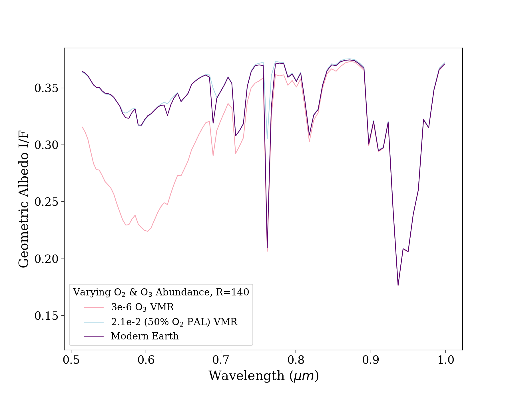
Figure 1: Reflection spectra of a modern-Earth atmospheric composition but with varied O3 and O2 abundances. We feature a high O3 abundance (3$\times 10^{-6}$), a 50% PAL O2 abundance (2.1$\times 10^{-2}$), and a modern Earth (7$\times 10^{-7}$ O3, and 2.1$\times 10^{-1}$ O2), respectively. All spectra are binned at R=140.

In the search for signs of planetary habitability, the detection of potential biosignatures can hint at biological activity on the planetary surface. Since Earth is currently our only example of a conclusively habitable (and inhabited) planet, using model scenarios with conditions similar to those on modern Earth or its distant past serves as a starting point for examining the detectability of planetary characteristics (Arney et al., 2016; Rugheimer & Kaltenegger, 2018). In particular, at different times in its history Earth hosted varying concentrations of the atmospheric biomarkers O2 and O3, which are primarily produced on Earth through photosynthesis and subsequent photochemical reactions; therefore measurements of geochemical proxies for the oxygenation of Earth’s surface and atmosphere over time provide examples of possible global biogeochemical scenarios that we could encounter when observing Earth-like exoplanets. It is also useful to consider planets that - like Earth - have global liquid water oceans, but no biospheres. In some conditions, such

The Phanerozoic (modern) epoch of Earth (541 million years ago – present), which forms the basis for most habitability and biosignature studies, has relatively high levels of both O2 (21%) and O3 (0.7 ppm) generated by abundant plant life and subsequent photochemistry. However, in the Proterozoic epoch (2.5 billion – 541 million years ago), photosynthetic life was less abundant and measurements suggest oxygen accumulation in the atmosphere at approximately 0.1% to 1% of modern Earth O2 levels but with potentially detectable levels of O3 (Planavsky et al., 2014). In a planetary atmosphere similar to the Archean epoch of Earth (4 – 2.5 billion years ago), we would expect an oxygen-poor and ozone-poor atmosphere, with a large abundance of greenhouse gases including CO2 and CH4, which may have in turn formed a photochemical organic atmospheric haze (Zerkle et al., 2012; Arney et al., 2016; Krissansen-Totton et al., 2018). In addition to past epochs of Earth’s history, models of alternative atmospheric scenarios are capable of producing of O2 and O3 dramatically higher than today’s values - even without the presence of biology - due to a variety of mechanisms (Hu et al., 2012; Domagal-Goldman et al., 2014; Gao et al., 2015; Tian, 2015; Harman et al., 2018).

As shown in Figure 1, we can see how varying the abundances of O2 and O3 can alter the resultant visible spectra and lead to differences in the detectability of these gases. In this work we quantify the detectability of O2 and O3, using reflected-light measurements at visible wavelengths (0.515 – 1 m), for a range of abundance values and spectral bandpasses. This project is a direct continuation from Latouf et al. (2023, hereafter BARBIE1) - in BARBIE1, we studied the detection of H2O as a function of SNR and abundance throughout the visible spectral range, and in this paper we extend the same methodology to the study of O2 and O3 and also examine the impact of the width of spectral bands on the SNR required for detection.In $[\S]$ 2 we present the methodology of our simulations, also providing a brief summary of BARBIE1. In $[\S]$ 3 we present the results of our simulations for both the modern Earth-like SNR study and the molecular abundance study. In $[\S]$ 4 we discuss the presented results and analyze the impact for future observations of varying Earth-twin epochs. In $[\S]$ 5 we present our conclusions and ideas for future work.

2 Methodology

We follow a similar methodological approach to that of BARBIE1. Herein we present a summary of the main steps in our analysis.

2.1 Inputs

2.1.1 Pre-Computed Spectral Grid

We use a geometric albedo spectral grid that was pre-computed by Susemiehl et al. (2023, hereafter S23). This grid is housed in the Planetary Spectrum Generator (PSG, Villanueva et al., 2018, 2022). The grid contains 1.4 million geometric albedo spectra that have been pre-computed with the parameters, minimum, and maximum values laid out in Table 1 of S23. The native resolution of the grid is set to R=500 and binned to R=140 for our analysis. For more information on the creation and verification of the grid, see S23 and BARBIE1. There are three molecular species in the grid: H2O, O3, and O2, with N2 as the assumed background gas. The minimum and maximum grid values for these parameters are as follows: H2O in [$10^{-8}$, $10^{-1}$]; O3 in [$10^{-10}$, $10^{-1}$]; O2 in [$10^{-10}$, $0.8$]; N2 = 1 - H2O - O3 - O2. The model is comprised of 50% clear and 50% cloudy spectra, i.e. $\mathrm{C_{f}}$ = 50%. There are three planetary parameters in the grid: surface pressure ($\mathrm{P_{0}}$), surface albedo ($\mathrm{A_{s}}$), and gravity (g). The minimum and maximum values for these parameters are as follows: $\mathrm{P_{0}}$ in [$10^{-3}$ Bar, 10 Bar]; $\mathrm{A_{s}}$ in [$10^{-2}$, 1]; gravity in [1 m/s², 100 m/s²]; and $\mathrm{R_{p}}$ is fixed to 1 $R_{\earth}$. The grid covers a wavelength range from 0.515 – 1.0 m as this range has been defined as the VIS channel in the exoplanet imaging instrument concepts studied in the Astro2020 Decadal Survey that form the starting point for HWO.

Log-Step O2	O2 (VMR)
0	2.1$\times 10^{-1}$†
-0.25	1.2$\times 10^{-1}$
-0.5	6.7$\times 10^{-2}$
-0.75	3.8$\times 10^{-2}$
-1	2.1$\times 10^{-2}$
-1.25	1.2$\times 10^{-2}$
-1.5	6.7$\times 10^{-3}$
-2	2.1$\times 10^{-3}$
-2.5	6.7$\times 10^{-4}$
-3	2.1$\times 10^{-4}$

Table 1: The above values were used in our simulations for O2, moving from Earth-like values into different epochs of Earth’s history.
^† Modern Earth-like value.

Log-Step O3	O3 (VMR)
+0.65	3$\times 10^{-6}$
+0.55	2.5$\times 10^{-6}$
+0.45	2$\times 10^{-6}$
+0.35	1.5$\times 10^{-6}$
+0.25	1.25$\times 10^{-6}$
+0.15	1$\times 10^{-6}$
+0	7$\times 10^{-7}$†

Table 2: The above values were used in our simulations for O3, moving from Earth-like values up to a high-O3 build-up regime.
^† Modern Earth-like value.

2.1.2 Mock Data and Retrieval Methodology

Our fiducial “data” spectrum is primarily set as a modern-Earth twin following Feng et al. (2018), with constant volume mixing ratios (VMRs) H2O$=3\times 10^{-3}$, O3$=7\times 10^{-7}$, O2=$0.21$, a background gas of N2=$1-$H2O$-$O3$-$O2, constant temperature profile at 250 K, $\mathrm{A_{s}}$ of 0.3, $\mathrm{P_{0}}$ of 1 Bar, and a planetary radius fixed at $\mathrm{R_{p}}$ = 1 $\mathrm{R_{\earth}}$. We consider a resolving power of 140, binned from the native grid resolving power of 500. This fiducial spectrum is given as data to the nested sampler in conjunction with the grid. We use the modern-Earth twin fiducial spectrum for our initial SNR study, wherein we focused on SNRs 3–16 moving in steps of 1. We then change the fiducial spectrum for our abundance study, changing only the molecule of interest one at a time, to the values listed in Table 2 and  2. All other parameters were left to modern-Earth values, in order to specifically constrain the molecule of interest. In BARBIE1, we focused on H2O, centered on modern-Earth values and moving in increasing and decreasing log-steps. This was due to the lack of constraint on H2O abundance throughout time. In this study, we consider O2 and O3, and set our maximum O2 value as the modern-Earth value of 0.21 VMR and move in decreasing log-steps of 0.25 and 0.5 down to values of 1% to 0.1% to represent a mid-Proterozoic Earth epoch (Planavsky et al., 2014). For O3 we wished to test the possibility that values higher than on modern-day Earth might present stronger detectability. To study this potential, we set the maximum value as 3 $\times 10^{-6}$ VMR, a value that is $\sim 5$x the modern-Earth value of 7 $\times 10^{-7}$ VMR, and well within the values created in models with high rates of abiotic O2 and O3 production on planets around F-, K, or M-type stars (Hu et al., 2012; Domagal-Goldman et al., 2014; Gao et al., 2015; Tian, 2015; Harman et al., 2018). and decrease to the minimum value as the modern-Earth value.In log space, we decreased in steps of 0.1, due to the small gap between the maximum and minimum values.

As in BARBIE1, to examine the detectability of the molecular species as a function of the central wavelength and width of a bandpass, we chose 25 evenly spaced values for the bandpass central wavelength. However, in this study we also vary the total width of the spectral bandpass, examining values of 20%, 30%, and 40%. These ranges are consistent with the simultaneous bandpasses that may be achieved with future high-performance coronagraphs (Ruane et al., 2015; Por, 2020; Juanola-Parramon et al., 2022). Using these bandpass values and the inputs laid out in 2.1.1 and 2.1.2, we run a series of Bayesian nested sampling retrievals for each abundance and SNR combination using the PSGnest application for the Planetary Spectrum Generator (PSG; Villanueva et al., 2018, 2022).

PSG is a radiative transfer model and tool for synthesizing and retrieving upon planetary spectra. This includes planetary atmospheres and surfaces covering wavelengths from 50 nm to 100 mm (i.e. from UV to Radio) and a large range of planetary properties. PSG includes aerosol, atomic, continuum, and molecular scattering/radiative processes, implemented layer-by-layer. PSG also includes the nested sampling routine PSGnest , which is an adaptation of the algorithm used in Fortran MultiNest (Feroz et al., 2009). PSGnest is a Bayesian retrieval tool based on the well-known MultiNest framework and designed for exoplanetary observations; for more information on PSGnest and our retrieval methodology, see S23 and BARBIE1.

2.2 Outputs

The output results file from PSGnest contains highest-likelihood values of output parameters, the average value resulting from the posterior distribution, uncertainties which are estimated from the standard deviation of the posterior distribution, and the log evidence (logZ) (Villanueva et al., 2022). It also includes the input data (wavelength, uncertainty, and input spectrum, in respective columns) with the best-fit spectrum. We calculate the median values, as well as the upper and lower limits of the 68% credible region (Harrington et al., 2022) using the output results. We also extract the posteriors and global log-evidence for use in our detectability calculations, which is the numerical representation that quantifies the relative support per each model given the input data (Feroz et al., 2009). Using these outputs, we compute the Bayes factor. The Bayes factor is calculated by subtracting the Bayesian log-evidence per retrieval using the fiducial gas abundances. The resulting differences are referred to as the log-Bayes factor ($\mathrm{lnB}$; Benneke & Seager, 2013). The log-Bayes factor determines which scenario is most likely by examining the hypothesis where all parameters are present, and systematically subtracting the evidences from scenarios where each parameter in turn is nullified. In our studies, if $\mathrm{lnB}$ is less than 2.5, it represents an unconstrained detection; if $\mathrm{lnB}$ is between 2.5 and 5, it is a weak detection; if $\mathrm{lnB}$ is greater than 5, it is a strong detection (reference Table 2 of Benneke & Seager, 2013). This differs slightly from Table 2 of Benneke & Seager (2013), in which $\mathrm{lnB}$ represents a weak, moderate, and strong detection respectively. We do not calculate the log-Bayes factor for non-gaseous components, as those factors cannot be absent and thus the calculation cannot represent a detection of those components.

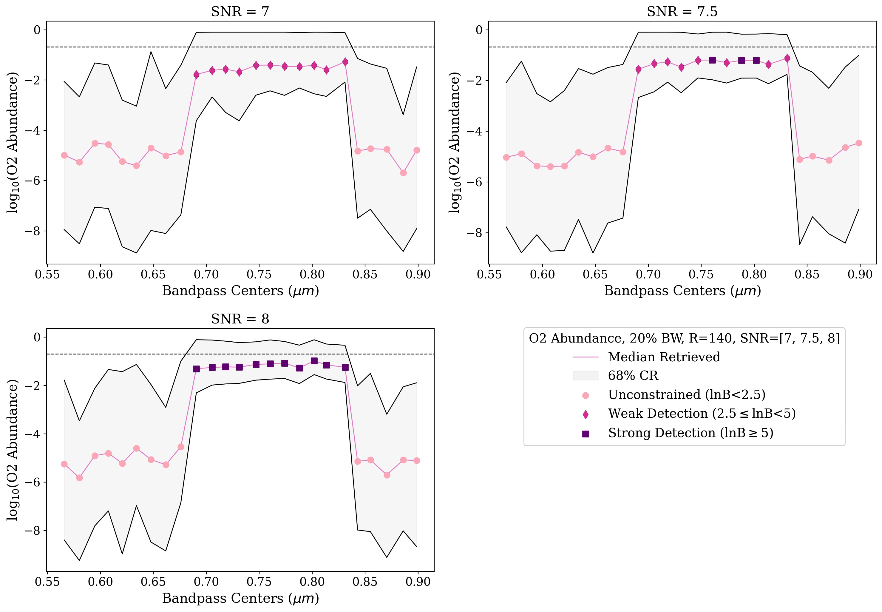
Figure 2: Results of the fiducial case study for O2, but showing only a narrow range of SNR values. The y-axis shows the abundance values for each molecule in log scale, with the true value is shown with the black dashed line (in this case, a modern Earth-like O2 value of 0.21 VMR). Each dot represents a bandpass center, with the pink line portraying the median retrieved values of O2 abundance for that bandpass, and the gray shaded region representing the upper and lower limits for the 68% credible region. Increased retrieval certainty can be seen where the gray regions narrow. Each point is colored to indicate varying detection strength. Unconstrained regions ($lnB<2.5$) are shown in light pink dots, weak detections ($2.5\leq lnB<5$) are shown in dark pink diamonds, and strong detections ($lnB>5$) are shown in purple squares. We present the range at which detectability materially changes for O2.

Figure 3: Results of the fiducial case study for O3 but focused on a specific narrow SNR range. We show the SNR range at which detectability materially changes for O3. All facets of the plot remain the same as in Figure 2. We notice that for SNR=20, 3 bandpasses achieve a strong detection but none of these bandpasses correctly constrain the abundance of O3 within the 68% credible region. We present further investigation on this in Figure 4.

Figure 4: Corner plots for O3 at 0.64 m at SNR=20 to portray the lack of continuum and its impact on O3 abundance retrieval. We also show a corner plot for SNR = 200 with all parameters set to exact grid points to portray the interpolation error in $A_{s}$. The 68% credible region is shown as pink shading in the 1D marginalized posterior distributions along the diagonal of the corner plot, and the true values are represented by black lines in the diagonals of the corner plot, and black stars within the 2D plots. It is clear that the error in A_S is due to a combination of parameter degeneracy and interpolation error in the grid-derived forward models.

3 Results

3.1 Modern Earth Case Results

We begin by presenting the detectability of O2 and O3 as a function of SNR for the fiducial modern-Earth case, as first examined by S23 and BARBIE1; all of the O2 and O3 data and calculated log-Bayes factors across abundance, SNR, and wavelength are available to the community on Zenodo. We only present the narrow SNR range within which detectability strength changes materially for O2 and O3 in Figures 2 and 3. We can see that based on Figure 2, for SNR $\leq 7$ there is only a weak or unconstrained detection possible for O2. However, beginning at SNR = 7.5, we can see strong detections of O2 corresponding to bandpasses containing deep O2 spectral features, such as at 0.74 m. A strong detection of O2 becomes possible from 0.68 - 0.84 m by SNR = 8. At SNRs higher than 8, all bandpass locations yield a strong detection of O2 with increasingly better constraints of the 68% credible region.

Looking to Figure 3, it was required to significantly increase the SNR to achieve a strong detection for O3. We look at an SNR range of 18 – 20, which is quite high, however it is only at this point that we begin to see a strong detection of O3 within the wavelength range of our simulations. At an SNR of 18, we can see a small area of weak detection between 0.6 and 0.67 m covering six bandpasses. At an SNR of 19, strong detection becomes possible for two bandpasses, and three bandpasses at SNR of 20. We can see it takes a very high SNR to achieve a strong detection of O3, which would lead to an exceptionally high integration time.

We can also see that although three bandpasses yield a strong detection at SNR=20, none of those bandpasses correctly constrain the abundance of O3 within the 68% credible region. We present further investigation on this in Figure 4a. In this corner plot, which is focused on 0.64 m at a 20% bandpass, O3 is not retrieved within the 68% credible region, and there is a large spread of the high probability region which does not center on the true value of O3. This is largely due to the lack of continuum caused by the depth and width of the ozone features; a similar problem for detecting H2O at long wavelengths is discussed at length in BARBIE1. We present Figure 4b to show that by increasing the bandpass width from 20% to 40% centered on 0.64 m, and thus increasing the amount of spectral region covered in each bandpass, an adequate continuum is constrained and the retrieval of O3 is firmly within the 68% credible region with little spread in the high probability regions.

However, we can see in the corner plots shown in Figure 4a and 4b that $A_{s}$ is also consistently retrieved at a value at least a factor of two away from the true value. To investigate the source of this incorrect retrieved parameter, we ran several retrievals with very high SNR (200) and with a data spectrum using values centered on a grid point, and compared both sets of results to our lower-SNR modern-Earth results. This allowed us to test whether the result was due to degeneracies for lower-SNR data or due to the impact of interpolation error in our grid-based retrieval scheme (as examined by S23). In Figure 4c, where we use a very high SNR and all of the parameters are set to exact values found in the S23 grid, we can see that all parameters are retrieved within a 68% credible region except for $C_{f}$ which is known to be degenerate. When $C_{f}$ is locked to its true value (0.5) as in Figure 4d, we can see this issue disappears and the range in the highest likelihood region decreases. There is higher interpolation error in $A_{s}$ likely due to the scarce sampling in the grid points and the limited bandwidth of the sampled spectra considered here. As there is only three grid points in this parameter space, there is a higher likelihood for interpolation error as there is more distance between the given true value and the nearest grid point. For a more in-depth description of this interpolation error and its impact, see S23.

In Figure 5 we present the shortest wavelength at which a weak or strong detection is achieved for O2 and O3; as described in BARBIE1, this is an important metric since the number of planets amenable to high-contrast coronagraphic imaging is higher when observing at shorter wavelengths due to the smaller inner working angle. Figure 5a provides a summarial result of Figures 2 and 3, covering the full range of SNR from 3-20 at a 20% bandpass. In Figure 5b, we present the shortest wavelength for strong detection if we assume a 30% bandpass, while in Figure 5c we present the shortest wavelength for strong detection if we assume a 40% bandpass. We also present the range for a strong detection of H2O as in BARBIE1, with additional SNRs to 20, to provide context to the results and present the possibilities for dual or triple molecule detection. To show the full range, we shade out to the longest wavelength where detection is possible.

Figure 5: In all panels, the shortest bandpass center at which one can achieve a strong detection for O2, or a strong or weak detection for O3 are shown in purple triangles, dark purple diamonds, and light pink dots respectively. The strong detection range for H2O is presented in pink squares, to provide context for dual or triple molecule detection. The range between the shortest and longest bandpass center at which detection is possible is filled in. We present the range for a strong detection SNR is on the y-axis, and the bandpass centers are on the x-axis. Note that the last bandpass center for strong detection is shaded out to the long edge of the bandpass, to maintain ability to directly compare the panels.

In Figure 5a we can see that O3 is only detectable, whether weakly or strongly, with high SNR ($\geq 14$) data over a very narrow range. We can see that O3 can be detected (albeit weakly) simultaneously with a strong detection of H2O at high SNR ($\geq 17$) with careful bandpass selection. However, the high SNR required for detection indicates that this would be costly in terms of observing time. Conversely, O2 is strongly detectable at an SNR of 8, with the range between shortest and longest wavelength encompassing all O2 features in the visible wavelength range. This detectability range overlaps significantly with the strong detection range of H2O. We can see that O2 and H2O can be simultaneously observed with SNR = 10 with careful selection of wavelength and corresponding bandpass. This also allows for a range of possible SNR depending on the desired wavelength of detection - if a longer wavelength such as 0.83 m is accessible, then SNR = 10 would allow for a dual detection, but if a short wavelength such as 0.68 m is required, then a much higher SNR is required. Next looking to Figure 5b, we see the detectability change, with triple molecule detection possible from a shortest wavelength of 0.66 m out to 0.7 m at an SNR $\geq 13$. O2 remains strongly detectable beginning at an SNR of 8 as in Figure 5a; however, while the shortest wavelength of detectability for O2 starts at approximately 0.69 m with a bandpass of 20%, the shortest wavelength of detectability for O2 with a bandpass of 30% starts at approximately 0.66 m. When we look to Figure 5c, we see that detectability changes drastically, with triple molecule strong detection possible from a shortest wavelength of 0.625 m out to 0.725 m at an SNR $\geq 11$. We can also see that once again, O2 remains strongly detectable beginning at an SNR of 8 as in Figure 5a and 5b, the shortest wavelength of detectability for O2 changes once more, starting at approximately 0.625 m with a bandpass of 40%. Thus, although the SNR of strong detectability does not change, the minimum possible wavelength of strong detectability significantly decreases as a function of bandpass width.

3.2 Results for Varying Abundance Cases

Figure 6: Shown above is the lowest SNR values for strong detection of the 0.74 m O2 feature as a function of O2 abundance. We note that although the 0.1% and 1% modern O2 abundances (i.e. mid-Proterozoic abundances) are in our study, they are not presented on the plot. We denote these abundances with a pink arrow. The VMR values are on the x-axis, with SNR on the y-axis. Strong detection is shown in purple squares, weak detection is shown in pink dots, the modern abundance range is highlighted with a light pink strip.

At this point in our study, we shift to present our abundance case study, wherein we vary the abundance of O2 below modern-Earth values and O3 above modern-Earth values. To assess the trade-off between longer observations (i.e., higher SNR) and different concentrations of O2 and O3, we varied the SNR on the observations for the full range of different VMRs per molecule. In Figure 6a, 6b, and  6c, we display the minimum SNR required to achieve a strong detection for each abundance of O2 at 0.76 m at 20%, 30%, and 40% bandpasses respectively. Looking first to Figure 6a, we notice that O2 quickly requires mid- to high-SNR data to be strongly or weakly detected with even one order of magnitude decrease in abundance. In fact, many of the abundances in our simulation are not detectable at all in this SNR range. The Proterozoic abundances of O2 (0.1% to 1% of modern Earth abundance) are not detectable at any SNR $\leq 20$, and in fact will likely require an extremely high SNR to become detectable, as these values are two to three magnitudes lower than modern Earth abundance values. As seen in Figure 6b, varying the bandpass to 30% decreases the required SNR for detection across almost all abundances of O2. For instance, where at a 20% bandpass it requires an SNR of 19 to strongly detect O2 at 2.1$\times 10^{-2}$ VMR, with a 30% bandpass the required SNR drops to 18. This is true for all detectable abundance cases except modern Earth values, which consistently requires an SNR of 8 for strong detection. In Figure 6c, we do not see a difference in required SNR for strong detection with a 40% bandpass.

While bandpass width makes little difference to the detectability of O2, it makes a significant difference when detecting O3. We can see in Figure 7 the large impact of the change in bandpass width. With a 20% bandpass centered on the 0.76 m O2, we capture the entirety of the O2 feature, along with the two smaller H2O features at 0.74 and 0.84 m. When the bandpass is widened to 40%, we capture all off the above, along with a portion of both the O3 feature that peaks at approximately 0.63 m and the 0.9 m H2O feature. In Figure 8a, 8b, and 8c, we display the minimum SNR required to achieve a strong detection for each abundance of O3 at 0.64 m with 20%, 30%, and 40% bandpasses respectively. In Figure 8a, we can see that O3 is detectable, strongly and weakly, in the full range of our simulation values. At modern Earth abundances, the required SNR for a strong detection is high at 19, but it is possible to achieve a weak detection at SNR = 14. When we increase to high O3 values, approximately 5x higher in abundance than modern Earth, the required SNR drops drastically, with strong or weak detection requiring SNRs of 7 or 5 respectively. The largest decrease in required SNR occurs between modern Earth values (7$\times 10^{-7}$ VMR) and 1.25$\times 10^{-6}$ VMR, dropping steeply from a required SNR of 19 to 11 for a strong detection, and 14 to 9 for a weak detection. When we increase the bandpass width to 30% as in Figure 8b, we see the required SNR for detection drop across all abundance values. For instance, at 1.5$\times 10^{-6}$ VMR, the required SNR for strong detection at a 20% bandpass is 10, with a 30% bandpass the required SNR drops to 8. This is true for all values across the abundances cases, to varying degrees of severity. This happens once more when the bandpass is widened to 40% as in Figure 8c. Looking to the same example case of 1.5$\times 10^{-6}$ VMR, the required SNR for strong detection drops to 6 at a 40% bandpass. With each increase of bandpass width, strong detectability at mid-low SNR data becomes more accessible, with a required SNR as low as 4 for a strong detection at 3$\times 10^{-6}$ VMR.

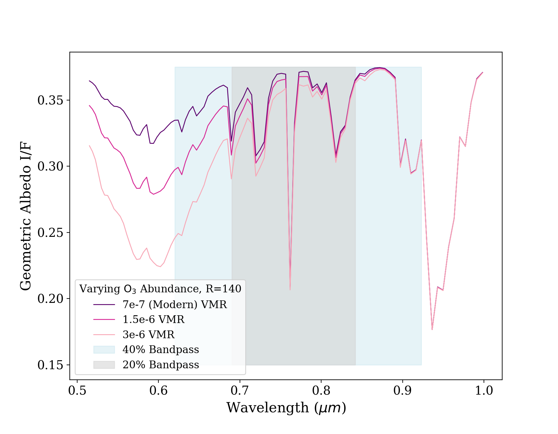
Figure 7: Spectra with varied O3 abundances. We feature the highest abundance (3$\times 10^{-6}$), the mid point abundance (1.5$\times 10^{-6}$), and lowest abundance in the study (7$\times 10^{-7}$) (modern Earth), respectively. All spectra are binned at R=140. We also present a 20% and 40% bandpass range width, in light grey and light blue respectively.

Figure 8: Shown above is the lowest SNR values for strong detection of the 0.63 m O3 feature as a function of O3 abundance. The VMR values are on the x-axis, with SNR on the y-axis. Strong detection is shown in purple squares, weak detection is shown in pink dots, and the modern abundance range is highlighted with a light pink strip.

3.3 Self-Consistent Chemistry Comparison

Parameter Symbol	Fiducial	New Values
$\mathrm{C_{f}}$	0.5
H2O	3$\times 10^{-3}$ VMR
O3	7$\times 10^{-7}$ VMR	105%, 110%, 105% PAL
O2	0.21 VMR	10%, 50%, 75% PAL
$\mathrm{P_{0}}$	1.0 Bar
$\mathrm{g}$	9.8 m/s
$\mathrm{A_{s}}$	0.3

Table 3: New input data spectrum values for the chemically consistent retrievals, following the Atmos values found in Kozakis et al. (2022) for O2 and O3

Figure 9: The shortest bandpass center at which one can achieve a strong detection for O2 or O3 at varying present atmospheric levels (PALs) for a specific SNR are shown in purple triangles and dark purple diamonds respectively. The range between the shortest and longest bandpass center at which detection is possible is filled in. The strong detection range for H2O is presented in pink squared to provide context to the results.

Figure 10: Shown above are the regions of single, dual, and triple molecular detection as a function of wavelength. wavelength is presented on the x-axis, SNR is presented on the y axis. The hatched regions symbolize regions with single molecule detection, shaded regions symbolize only the overlapping areas between dual molecular strong detection zones, and the black outlined shaded regions symbolize the overlapping areas between triple molecular strong detection. We present the 10% O2 PAL and 105% O3 PAL case in the first row, the 50% O2 PAL and 110% O3 PAL case in the second row, and the 100% O2 PAL and 100% O3 PAL case in the last row. For all cases, we present a 20%, 30%, and 40% bandpass width.

As previously discussed, in our previous simulations we varied one molecular abundance (for O2) while the other parameters were held fixed to modern Earth-like values, thus we did not explore the relationship between varying both O2 and O3 and the resultant change in detectability. However, due to the photochemical relationship between the O2 abundance and the production of O3, the abundances of both molecules would actually be linked in any atmospheric scenario. As found in Kozakis et al. (2022), the relationship between O2 and O3 varies for model atmospheres depending on the type of host star, and the linearity of the relationship also appears to vary. When looking to hotter host stars (e.g., a G2 star), peak O3 abundance occurs at lower than modern Earth O2 abundances due to the O3 layer shifting in the atmosphere downwards to O2 levels due to O2 photochemical shielding.

This O2/O3 relationship means that we can constrain the overall molecular oxygen abundance by detecting either of the species; O3 is in fact a highly sensitive tracer of lower abundances of O2. In order to explore the impact of this, we examined several scenarios where we varied our parameter values as coupled parameters, i.e. 10% PAL O2/105% PAL O3, etc., consistent with the results for a Sun-like star from Kozakis et al. (2022) (as seen in Table 3). We present our detectability results for these abundance pairs in Figure 9. In Figure 9a-c, we present the O2 results with H2O at 20%, 30%, and 40% bandpasses at 10% PAL, 50% PAL, and 75% PAL of O2. We can see that at 10% PAL, O2 detectability is unlikely, requiring a minimum SNR of 19 at a 20% bandpass, and SNR of 18 at 30% and 40% bandpasses. However, between 50% PAL, 75% PAL, and the previously presented 100% PAL of O2, there are little difference, with slight variance in SNR (e.g. from requiring SNR of 8 for 100% PAL O2 to requiring SNR of 10 for 50% PAL O2) and little change across bandpass width as in Figure 5. In Figure 9d-f, we present the O3 results with H2O at 20%, 30%, and 40% bandpasses at 105% PAL and 110% PAL of O3. We can see that detectability does not shift significantly for O3, as our values do not vary greatly from a modern-Earth like value. However, one notable difference is that there is a larger range for strong O3 detection at both 105% and 110% O3 PAL with bandpass width 20% than the same bandpass width with 100% O3 PAL as in Figure 5. We also see that O3 is detectable at an SNR of 17 rather than 19 as in the modern-Earth like results for a 20% bandpass. The detectability range of O3 increases with increasing bandpass width, as expected following Figure 5.

Following this, we analyze the limiting molecule in double or triple molecular detection in Figure 10. We present 10% O2/105% O3 PAL in Figure 10a-c. We can see that detection of O2 dually or triply with H2O or O3 is difficult. At a 20% bandpass, H2O and O2 are dual detectable only at an SNR $\geq 19$. At a 30% bandpass, triple H2O/O2/O3 detection is possible at an SNR $\geq 18$ in a very narrow wavelength range (approximately 0.66 to 0.7 m), and dual H2O/O2 detection is also possible at an SNR $\geq 18$, while dual H2O/O3 detection has a wider range of detectability, from SNR $\geq 14$, and from approximately 0.63 to 0.7 m. At a bandpass of 40%, the range for triple detection increases in wavelength, to approximately 0.63 to 0.76 m. The range for dual H2O/O3 detection also increases, starting from SNR $\geq 11$ and from 0.63 to 0.75 m. At all bandpasses, H2O has a large range in wavelength and SNR of single detectability thus it is highly likely to strongly detect H2O. In all bandpasses, O2 is the limiting molecule for dual or triple detection in both SNR and wavelength. In terms of dual H2O/O3 detection, O3 is the limiting molecule in wavelength, but H2O is the limiting molecule in SNR.

We present 50% O2/110% O3 PAL in Figure 10d-f. We can see that, as in the modern Earth case, dual detection of H2O and O2 is always possible at all bandpasses. The same is not true for H2O and O3 however, with dual strong detection possible at only a single point in the 20% bandpass, and with a wider range possible at 30%. At 40%, there is no dual detection of H2O and O3, however there is a large range (approximately 0.12 m in width) wherein triple detection is possible from SNR $\geq 11$. At 30% and 40% bandpasses there are also areas where dual detection is possible with O2 and O3 at mid-high SNR and short wavelengths. With a 20% bandpass, H2O is the limiting molecule for dual H2O/O2 detection in both SNR and wavelength. At a 30% bandpass, H2O is still the limiting molecule for dual H2O/O2 detection and triple H2O/O2/O3 detection in SNR, however O3 is the limiting molecule in wavelength. When looking at dual H2O/O3 detections, H2O is the limiting molecule in SNR and wavelength, mimicking the dual H2O/O2 detection. At a 40% bandpass, O3 is the limiting molecule in wavelength for a triple H2O/O2/O3 detection, and H2O is the limiting molecule in SNR for a triple H2O/O2/O3 detection. We then have the same H2O limiting for dual H2O/O2 detection in SNR, although there is no limiting molecule for dual detection in wavelength since the final bandpasses have detections for both H2O and O2.

We present 100% O2/100% O3 PAL in Figure 10g-i. In the 20% bandpass, we see extremely similar results to Figure 10d, with the notable difference that O2 detection is possible down to an SNR of 8, compared to an SNR of 10. In the 30% bandpass, we again see almost identical results to the 50% O2/110% O3 PAL case shown in Figure 10e. The differences here are once again that O2 is detectable down to an SNR of 8, but we also notice that O3 has a smaller region of single detectablity, which is also seen in the smaller region of dual O2/O3 detection. As a result of the lower SNR requirements for O2 detectability, this results in a large region of dual H2O/O2 detection. In the 40% bandpass, once again the results mimic the 50% O2/110% O3 PAL counterpoint case shown in Figure 10f. The differences shown are a smaller region of triple H2O/O2/O3 detection and dual O2/O3, resulting in larger single O2 and dual H2O/O2 detection regions. This also results in a smaller single H2O detection region. In these cases, the limiting molecules are the same as above: At a 20% bandpass, H2O is the limiting molecule for dual H2O/O2 detection in both SNR and wavelength. At a 30% bandpass, H2O is the limiting molecule for dual H2O/O2 detection and triple H2O/O2/O3 detection in SNR, however O3 is the limiting molecule in wavelength. At a 40% bandpass, O3 is the limiting molecule in wavelength and SNR for a triple H2O/O2/O3 detection.

4 Discussion

The primary utility of the retrieval results presented here is to help understand how the impact of O2 and O3 abundance affects the optimal strategy for detecting the presence of an atmosphere with water and oxygen with spectroscopic bandpasses in the visible-light spectral region. Here we discuss the major conclusions from this work, as well as some of the limitations to the study that may impact these conclusions.

The most important result is the role that the width of the bandpass plays. When examining Figures 6 and 8, we can see the notable difference in how a widening bandpass changes the detectability of molecules across abundance and type; where O2 detectability does not vary significantly as a function of bandpass across abundance values, O3 changes significantly as the bandpass widens. This is likely due to the fact that the O2 feature is narrow and deep, thus making it easily detectable at high abundance values, but easily captured in a smaller bandpass width, whereas O3 has a very broad feature thus the widening of the bandpass allows for a stronger continuum and significant change in detection as a function of bandpass. O3 also does not have any strong features in the 0.515 – 1 m region, leading to inherent difficulty in detection in this range. However, if we are able to observe the strong O3 band at 0.36 m, detection would become stronger at lower SNR data. Recent works, such as by Damiano et al. (2023), have investigated this principle and come to the conclusion that even with impacts of possible confusion due to SO2 and other species, O3 detection is indeed easier at lower SNR and lower resolution data. Damiano et al. (2023) found that with spectral resolution of 7, and SNR = 10, O3 can be detected in the UV at sub-PAL VMRs; they also note that observing additional signatures of habitability in the NIR region is crucial to interpreting O3 detections at UV and VIS wavelengths.We will examine these questions further in future work addressing the complete UV, VIS and NIR wavelength regions.

A wider bandpass also better enables detections of one or more molecules with a single bandpass - in particular, the detection of O3 with other molecules. In Figure 5, we can see that for modern Earth abundances a bandpass width of $\geq 30\%$ would allow for a detection of H2O at slightly shorter wavelengths (long-wavelength cutoff of $\sim$0.95 m versus 0.99 m for a 20% bandpass) and also a joint measurement of a strong O2 detection and at least a weak O3 detection with SNR = 8-9 versus only O2 (which could help to limit false positives and motivate additional observations). Furthermore, Figure 10 shows that a 40% bandpass width enables a significant improvement in the ability to detect all three species with a single bandpass at around 0.72 m; this could either be used alone as a first reconnaissance bandpass or could be used as the follow-up to a longer-wavelength search for H2O alone at low SNR. The optimal choice between these two options depends significantly on whether a planet is detectable at longer wavelengths (due to IWA) and whether the exposure time required for longer-wavelength measurements is significantly impacted by instrument sensitivity; we leave these instrument- and target-dependent considerations to future work.

The second important result is that the abundance versus SNR results in Figures 6 and 8 show a non-linear increase in the required SNR at smaller abundances. Combined with the fact that SNR is linearly dependent on the square of exposure time, this suggests that our exposure time will be extremely sensitive to the limiting abundance that must be detectable. Figure 10 further demonstrates this, showing that when O2 drops from 50% PAL (12% VMR) to 10% PAL (2% VMR), it essentially becomes undetectable. This motivates a deeper analysis of whether detecting O2 at visible wavelength should be a high priority in the progression of measurements if there is a high likelihood of a non-detection for even a moderate abundance, compared with a measurement of more sensitive markers of atmospheric abundance in the UV or NIR.

We note that high O3 abundances are challenging to model, in that it takes a very small amount to completely overwhelm the spectrum. Spectra with high O3 have continua near zero, which also causes the error value to increase substantially, thus high values of O3 must be handled with care. At high abundances, the error value increase can lead to poorly constrained retrievals using our grid. Susemiehl et al. (2023) found that this occurs at high O3 ($log_{10}\ce{O3}>-5$) concurrently occurring with low $\mathrm{P_{0}}$ ($log_{10}\mathrm{P_{0}}<-1.7$) using our grid. Our simulations go no higher than $log_{10}\ce{O3}\leq-6$ and therefore avoid this degeneracy and resulting poorly constrained retrievals.

As discussed in BARBIE1, there have been similar prior works that investigated the relationship between SNR and detectability, specifically Feng et al. (2018) and Damiano & Hu (2022). We explore the differences in retrieval parameterization structure in BARBIE1, however even with the differences in techniques and analysis, our results for O2 and O3 detectability are in agreement. An SNR of 10 at R = 140 is sufficient to firmly constrain the abundances for an Earth-twin atmosphere with O2 and O3. Our work also explores the influence of varying bandpass width on molecular detection, which varies from prior work, and thus presents a new analysis of detection possibilities.

5 Conclusions & Future Work

To summarize, by investigating bandpass width in tandem with SNR, we can see that detectability is intrinsically linked to both factors as an additional function of molecular type. The ability to properly prioritize and select the best combination of parameters can drive efficient observing practices. By understanding the SNR requirements for strong detection of O2 and O3 and also understanding which bandpass width could result in simultaneous strong detection of O2, O3, and H2O, we can properly prioritize the best combination of bandpass and required SNR for detection, thereby informing the best options for instrument design trades and observing procedure. O3 is most easily observable using a 30 or 40% bandpass width at shorter wavelengths with mid-low SNR data. With a 20% bandpass width, O3 is difficult to detect, requiring SNR $\geq 19$ at modern-Earth values. O2 is not significantly affected by bandpass width, and consistently requires an SNR of $\geq 8$ to be strongly detected at modern-Earth values at 0.76 m and shorter. It is not detectable at SNR $\leq 20$ at Proterozoic era abundances. Since the coronagraph and instrument capabilities may dictate that the best observation occurs at shorter wavelengths, O2 and O3 are well within the most optimized instrument capabilities. O2 and O3 have strong geochemical markers that provide a depth of knowledge to potential Earth observations, and a heightened ability to constrain the observed Earth-like epoch.

By also investigating coupled atmospheric abundances of O2 and O3, we can study how detectability of these molecules vary with the other parameter. Allowing parameters to vary with each other following leading coupled photochemistry and atmospheric models, we can prioritize the optimal bandpass width for more realistic exo-Earth simulations.

In future work, we plan to build a new spectral model grid that includes a wider range of molecular species, and we will extend to shorter and longer wavelengths than the visible range. Specifically, we will cover the same wavelengths as the proposed coronagraph instrument for the Habitable Worlds Observatory (Juanola-Parramon et al., 2022), including UV, Optical, and NIR. This will allow us to study more biosignatures and molecular species of interest, and represent the physical chemistries more accurately. This will allow us to expand our simulations of possible observations and establish best observational practices for exoEarth observations using next generation telescopes. We will also develop a PSG module to display all detectability information in a publicly accessible format. We note that SNR results may be subject to minor changes following grid reconstruction due to PSG radiative transfer upgrades. We will also include a full exoplanet yield calculation using the data contained within BARBIE1 and BARBIE2 to give an educated baseline for detection of biomarkers. The interpolation metric used in this work is a trilinear interpolation scheme which can be used on 3D grids as in this work, but in future works we will investigate if another interpolation metric, such as inverse distance weighted interpolation or multiplicative weight interpolation, can minimize interpolation error in grid-based retrievals.

We will also conduct photochemically self-consistent studies in order to inform and broaden the results for future retrieval studies using grids. The expansion of grid parameter space will allow for the possibility of chemically consistent modeling, combined with input from updated photochemical models to ensure self-consistent atmospheric gas compositions with retrievals. This will be particularly important for considerations of gas detections for planets around different star types, given the impact star type has on the photochemistry of planetary atmospheres (Segura et al., 2005, 2010; France et al., 2012).

N. L. gratefully acknowledges financial support from an NSF GRFP. N.L. gratefully acknowledges Dr. Joesph Weingartner for his support and editing. N. L. also gratefully acknowledges Greta Gerwig, Margot Robbie, Ryan Gosling, Emma Mackey, and Mattel Inc.™ for Barbie (doll, movie, and concept), for which this project is named after. This Barbie is an astrophysicist! The authors also gratefully acknowledge conversation with Dr. Chris Stark regarding exoEarth yields and instrument design. The authors would like to thank the Sellers Exoplanet Environments Collaboration (SEEC) and ExoSpec teams at NASA’s Goddard Space Flight Center for their consistent support. MDH was supported by an appointment to the NASA Postdoctoral Program at the NASA Goddard Space Flight Center, administered by Oak Ridge Associated Universities under contract with NASA.

References

- Arney et al. (2016) Arney, G., Domagal-Goldman, S. D., Meadows, V. S., et al. 2016, Astrobiology, 16, 873, doi: 10.1089/ast.2015.1422
- Benneke & Seager (2013) Benneke, B., & Seager, S. 2013, ApJ, 778, 153, doi: 10.1088/0004-637X/778/2/153
- Charbonneau et al. (2002) Charbonneau, D., Brown, T. M., Noyes, R. W., & Gilliland, R. L. 2002, ApJ, 568, 377, doi: 10.1086/338770
- Damiano & Hu (2022) Damiano, M., & Hu, R. 2022, arXiv e-prints, arXiv:2204.13816. https://arxiv.org/abs/2204.13816
- Damiano et al. (2023) Damiano, M., Hu, R., & Mennesson, B. 2023, AJ, 166, 157, doi: 10.3847/1538-3881/acefd3
- de Wit et al. (2016) de Wit, J., Wakeford, H. R., Gillon, M., et al. 2016, Nature, 537, 69, doi: 10.1038/nature18641
- Domagal-Goldman et al. (2014) Domagal-Goldman, S. D., Segura, A., Claire, M. W., Robinson, T. D., & Meadows, V. S. 2014, ApJ, 792, 90, doi: 10.1088/0004-637X/792/2/90
- Feng et al. (2018) Feng, Y. K., Robinson, T. D., Fortney, J. J., et al. 2018, AJ, 155, 200, doi: 10.3847/1538-3881/aab95c
- Feroz et al. (2009) Feroz, F., Hobson, M. P., & Bridges, M. 2009, MNRAS, 398, 1601, doi: 10.1111/j.1365-2966.2009.14548.x
- France et al. (2012) France, K., Linsky, J. L., Tian, F., Froning, C. S., & Roberge, A. 2012, ApJ, 750, L32, doi: 10.1088/2041-8205/750/2/L32
- Gao et al. (2015) Gao, P., Hu, R., Robinson, T. D., Li, C., & Yung, Y. L. 2015, ApJ, 806, 249, doi: 10.1088/0004-637X/806/2/249
- Gaudi et al. (2020) Gaudi, B. S., Seager, S., Mennesson, B., et al. 2020, arXiv e-prints, arXiv:2001.06683, doi: 10.48550/arXiv.2001.06683
- Harman et al. (2018) Harman, C. E., Felton, R., Hu, R., et al. 2018, ApJ, 866, 56, doi: 10.3847/1538-4357/aadd9b
- Harrington et al. (2022) Harrington, J., Himes, M. D., Cubillos, P. E., et al. 2022, \psj, 3, 80, doi: 10.3847/PSJ/ac3513
- Hu et al. (2012) Hu, R., Seager, S., & Bains, W. 2012, ApJ, 761, 166, doi: 10.1088/0004-637X/761/2/166
- Juanola-Parramon et al. (2022) Juanola-Parramon, R., Zimmerman, N. T., Pueyo, L., et al. 2022, Journal of Astronomical Telescopes, Instruments, and Systems, 8, 034001, doi: 10.1117/1.JATIS.8.3.034001
- Kaltenegger (2017) Kaltenegger, L. 2017, ARA&A, 55, 433, doi: 10.1146/annurev-astro-082214-122238
- Kozakis et al. (2022) Kozakis, T., Mendonça, J. M., & Buchhave, L. A. 2022, A&A, 665, A156, doi: 10.1051/0004-6361/202244164
- Kreidberg et al. (2019) Kreidberg, L., Koll, D. D. B., Morley, C., et al. 2019, Nature, 573, 87, doi: 10.1038/s41586-019-1497-4
- Krissansen-Totton et al. (2018) Krissansen-Totton, J., Olson, S., & Catling, D. C. 2018, Science Advances, 4, eaao5747, doi: 10.1126/sciadv.aao5747
- Latouf et al. (2023) Latouf, N., Mandell, A. M., Villanueva, G. L., et al. 2023, AJ, 166, 129, doi: 10.3847/1538-3881/acebc3
- Lim et al. (2023) Lim, O., Benneke, B., Doyon, R., et al. 2023, arXiv e-prints, arXiv:2309.07047, doi: 10.48550/arXiv.2309.07047
- Madhusudhan (2019) Madhusudhan, N. 2019, ARA&A, 57, 617, doi: 10.1146/annurev-astro-081817-051846
- Planavsky et al. (2014) Planavsky, N. J., Reinhard, C. T., Wang, X., et al. 2014, Science, 346, 635, doi: 10.1126/science.1258410
- Por (2020) Por, E. H. 2020, ApJ, 888, 127, doi: 10.3847/1538-4357/ab3857
- Roberge & Moustakas (2018) Roberge, A., & Moustakas, L. A. 2018, Nature Astronomy, 2, 605, doi: 10.1038/s41550-018-0543-8
- Ruane et al. (2015) Ruane, G. J., Huby, E., Absil, O., et al. 2015, A&A, 583, A81, doi: 10.1051/0004-6361/201526561
- Rugheimer & Kaltenegger (2018) Rugheimer, S., & Kaltenegger, L. 2018, ApJ, 854, 19, doi: 10.3847/1538-4357/aaa47a
- Seager & Deming (2010) Seager, S., & Deming, D. 2010, ARA&A, 48, 631, doi: 10.1146/annurev-astro-081309-130837
- Segura et al. (2005) Segura, A., Kasting, J. F., Meadows, V., et al. 2005, Astrobiology, 5, 706, doi: 10.1089/ast.2005.5.706
- Segura et al. (2010) Segura, A., Walkowicz, L. M., Meadows, V., Kasting, J., & Hawley, S. 2010, Astrobiology, 10, 751, doi: 10.1089/ast.2009.0376
- Susemiehl et al. (2023) Susemiehl, N., Mandell, A. M., Villanueva, G. L., et al. 2023, AJ, 166, 86, doi: 10.3847/1538-3881/ace43b
- The LUVOIR Team (2019) The LUVOIR Team. 2019, arXiv e-prints, arXiv:1912.06219. https://arxiv.org/abs/1912.06219
- Tian (2015) Tian, F. 2015, Earth and Planetary Science Letters, 432, 126, doi: 10.1016/j.epsl.2015.09.051
- Villanueva et al. (2022) Villanueva, G. L., Liuzzi, G., Faggi, S., et al. 2022, Fundamentals of the Planetary Spectrum Generator (Self-Published)
- Villanueva et al. (2018) Villanueva, G. L., Smith, M. D., Protopapa, S., Faggi, S., & Mandell, A. M. 2018, J. Quant. Spec. Radiat. Transf., 217, 86, doi: 10.1016/j.jqsrt.2018.05.023
- Zerkle et al. (2012) Zerkle, A. L., Claire, M. W., Domagal-Goldman, S. D., Farquhar, J., & Poulton, S. W. 2012, Nature Geoscience, 5, 359, doi: 10.1038/ngeo1425
- Zieba et al. (2023) Zieba, S., Kreidberg, L., Ducrot, E., et al. 2023, Nature, 620, 746, doi: 10.1038/s41586-023-06232-z