Sparsify-then-Classify:
From Internal Neurons of Large Language Models
To Efficient Text Classifiers

Abstract

Among the many tasks that Large Language Models (LLMs) have revolutionized is text classification. However, existing approaches for applying pretrained LLMs to text classification predominantly rely on using single token outputs from only the last layer of hidden states. As a result, they suffer from limitations in efficiency, task-specificity, and interpretability. In our work, we contribute an approach that uses all internal representations by employing multiple pooling strategies on all activation and hidden states. Our novel lightweight strategy, Sparsify-then-Classify (STC) first sparsifies task-specific features layer-by-layer, then aggregates across layers for text classification. STC can be applied as a seamless plug-and-play module on top of existing LLMs. Our experiments on a comprehensive set of models and datasets demonstrate that STC not only consistently improves the classification performance of pretrained and fine-tuned models, but is also more efficient for both training and inference, and is more intrinsically interpretable.

$\star$ The authors contribute equally to this paper.

1 Introduction

Ever since the groundbreaking work of Vaswani et al. (2017), transformer-based models have rapidly become mainstream and firmly established the research forefront. Large Language Models (LLMs) have in recent years rapidly evolved into remarkably advanced and sophisticated tools with emergent capabilities that, in many cases, often rival or even surpass human performances across a spectrum of rather complex Natural Language Processing (NLP) tasks, including natural language inference, machine translation, text summarization, and question answering (Srivastava et al., 2022).

Despite the supreme performance in a wide variety of NLP tasks which is still not saturated with increasing parameters, researchers are currently facing with several pivotal challenges in applying novel advanced LLMs like GPT-4 to text classification tasks. Contemporary mainstream paradigms leveraging pretrained LLMs as text classifiers include sentence embedding, model fine-tuning and in-context learning, among which each paradigm, however, comes with its own set of limitations. In general,

• The sentence embedding approach directly using pretrained model outputs often results in suboptimal performance, as the entire sentence embedding process is designed to be task-agnostic.

• While the model fine-tuning approach frequently achieves state-of-the-art (SotA) performance in text classification tasks, it demands a substantial investment in computational resources and time, especially as model sizes grow. Additionally, the per-task-per-model nature often limits the model’s versatility, making it suitable only for the specific task it was fine-tuned for.

• The in-context learning (ICL), as exemplified by the few-shot prompting (Brown et al., 2020) that demands no explicit fine-tuning, has its own set of challenges. The effectiveness of ICL hinges critically on the quality of the prompts used, with performance varying dramatically from matching the SotA fine-tuned models to mere random guess, leading to the necessity of prompt engineering which can become an intricate and costly trial-and-error process (Lu et al., 2021, Liu et al., 2023).

Additionally, among all existing text classification paradigms, the vastly underlying implicit processes, by which the models achieve their prominent capabilities, have been inadvertently neglected, as shown in Figure 5. In specific, a common trait among the three conventional approaches is their naïve reliance on a single token output from the final layer’s hidden state output of the model, such as the first [CLS] token in BERT or the last token in GPT for each input sentence, which potentially loses task-specific information learned by the internal representations of the model. On the other hand, recent studies in LLM interpretability (Bills et al., 2023, Gurnee and Tegmark, 2023) have demonstrated that internal representations are remarkably adept at capturing essential features, yet barely have they explored the possibility of establishing better text classifiers from leveraging multi-layer representations.

Table 1: Baselines and Sparsify-then-Classify for LLM application in text classification

	Fine-tuning / (Re-)training
Approach	Prompt	Model Weights	Clf. Head	Structure Focus	Representation
Sentence Embedding	N	N	Y	encoder	single token last layer hidden states
Model Fine-tuning	N	Y	Y	all
In-context Learning	Y	N	N (LM head)	generative
Sparsify-then-Classify (proposed)	N	N	Y	encoder / decoder	multiple pooling layer aggregation hidden states & activations

Table 2: Performance and efficiency improvement of Sparsify-then-Classify in IMDb dataset

Metrics	DistilBERT	RoBERTa	GPT2	GPT2-M	GPT2-L	GPT2-XL
Performance boost on frozen models	+0.13%	+2.95%	+6.40%	+5.24%	+2.83%	+3.33%
Performance boost on fine-tuned models	+0.09%	+1.07%	+2.17%	+3.14%	+2.02%	+2.02%
est. number of trainable parameters	0.14%	0.18%	0.19%	0.24%	0.25%	0.25%
est. total training floating point operations	34.95%	34.98%	36.42%	36.29%	36.03%	35.51%

To address the aforementioned issues accompanied by traditional text classification approaches, in this work, we propose the Sparsify-then-Classify (STC) approach shifting focus from the final layer outputs to the rich internal representations within LLMs that could be utilized respectively for text classification tasks. As shown in Table 1, our method leverages activations of feedforward neural network (FFN) neurons within transformer blocks and hidden states across different layers of pretrained models, with neither the need for retraining or fine-tuning model weights nor prompt engineering. By investigating the massive internal representations hidden beneath model outputs, we sparsify salient features relevant to specific tasks using logistic regression probes, and subsequently develop aggregation strategies emphasizing the multi-layer representation of sparsified features to form task-specific classifiers.

Given that model structure and weights are transparent, STC can be seamlessly integrated into existing pretrained and fine-tuned transformer-based models in a plug-and-play fashion. Current results from our experiments on RoBERTa, DistilBERT, and GPT2 family, as Table 2 shows, demonstrate that our proposed approach not only consistently outperforms conventional sequence classification methods on both pretrained and fine-tuned models, but also achieves greatly improved efficiency. Specifically, when applied to a frozen pretrained GPT2-XL model for the IMDb sentiment classification task, our method, by aggregating only the activation results from the lower 60% layers yields a 94.72% accuracy that can already surpass the 93.11% of the fully fine-tuned model. Extending STC to all layers makes merely 0.25% of original trainable parameters and 35.51% of the training cost compared with fine-tuning baseline, with further boosting the performance to 94.92%, all from a frozen task-agnostic pretrained model.

The primary contributions of our work are as follows:

1. We propose a lightweight Sparsify-then-Classify method. After layer-wise linear probing on pooled FFN activation or hidden state patterns across layers of pretrained LLMs, we sparsify salient neurons on each layer and aggregate across layers to train a hierarchical text classifier.

2. We show that for different transformer-based LLMs, our approach consistently outperforms existing LLM application paradigms for text classification. Our method applying to frozen models yields results approaching or even surpassing the fine-tuned models, and deployed on already fine-tuned models could even further improve the performance.

3. Through comparative analyses, our method, when applied to well-established models, demonstrates improved performance compared with the best results independently derived from probing single layers, along with better efficiency in training and inference, and intrinsic interpretability.

2 Preliminaries

This section lays the groundwork for our exploration of transformer-based LLMs by delving into internal mechanisms and representations. We establish here the essential nomenclature and terminology to facilitate a clear and consistent understanding of the concepts and methodologies discussed throughout this study.

The foundational structures of transformer-based models, including encoder-only variants like BERT and decoder-only variants like GPT, always comprise three principal components: (1) an embedding layer at the base focusing on translating tokens into dense vectors within a high-dimensional hidden space, (2) $L$ identical encoder or decoder blocks, each of which contains a $H$-head (self-)attention mechanism and a feed-forward network (FFN), jointly applying nonlinear transformations on intermediate representations of $D$-dimensional hidden space, and (3) a head layer on top of the last-layer hidden states that reshapes and refines representation outputs to generate desired final output, for instance, language modeling head (LM head) in GPT for next token output, or sequence classification head for label output. An illustration is provided in A.1.

Encoder and Decoder Mechanisms

Raw texts tailored for specific tasks serve as inputs to the pretrained tokenizers before entering the language model. After going through model-specific word-token embedding and word-position embedding mechanisms, a tokenized input sequence of length $N$ becomes the first hidden state $\bm{X}_{0}\in\mathbb{R}^{N\times D}$ that works as the input to the block at layer $0$. Afterward, the inner mechanism of each transformer block at layer $l\in\{0,\cdots,L-1\}$ can be formulated as follows:

$$\bm{Q}_{l,h} =\bm{X}_{l}\bm{W}_{l,h}^{Q},\bm{K}_{l,h}=\bm{X}_{l}\bm{W}_{l,h}^{K},\bm{V}_{l,h}=\bm{X}_{l}\bm{W}_{l,h}^{V}$$

$$\text{Attn}_{l}(\bm{X}_{l}) =\bigoplus_{h=0}^{H}\text{Attn}_{l,h}(\bm{X}_{l})=\bigoplus_{h=0}^{H}\text{softmax}(\bm{Q}_{l,h}\bm{K}_{l,h}^{T})\bm{V}_{l,h}$$

$$\bm{H}_{l} =\bm{X}_{l}+\text{Attn}_{l}(\bm{X}_{l})$$

$$\text{FFN}_{l}(\bm{H}_{l}) =f_{\text{act}}(\bm{H}_{l}\bm{W}_{l,1}+\bm{b}_{l,1})\bm{W}_{l,2}+\bm{b}_{l,2}$$

$$\bm{X}_{l+1} =\bm{H}_{l}+\text{FFN}_{l}(\bm{H}_{l})$$

where matrices with $h\in\{0,\cdots,H\}$ represent different attention heads, $\text{Attn}_{l}(\bm{X}_{l})$ being formed by concatenating the (self-)attention output of all heads $\text{Attn}_{l,h}(\bm{X}_{l})$, $\bm{H}_{l}$ the attention output with residual added, which serves as input for FFN, whose output with residual added subsequently becomes the next hidden state $\bm{X}_{l+1}$. The scaling factors, layer norms, and dropouts are omitted here for simplicity.

Internal Representations

For each layer, we focus on the hidden state and activation records of $\text{FFN}_{l}$

$$\bm{X}_{l} \in\mathbb{R}^{N\times D},\qquad l=0,\cdots,L$$

$$\bm{A}_{l} =f_{\text{act}}(\bm{H}_{l}\bm{W}_{l,1}+\bm{b}_{l,1})\in\mathbb{R}^{N\times A},\qquad l=0,\cdots,L-1$$

in which $A=kD$ is by convention a multiple of $D$ representing the number of FFN neurons, i.e., the dimension of hidden space within the FFN.

The Head Layer

Conventionally, the hidden states in the last layer $L$ of each neuron are condensed token-wise across the entire input sequence with a variable sequence length $N$ into a feature space with a static size of $1$, by $f_{\text{single}}$ picking the result on the specific position at a certain single token, i.e. [CLS] at the beginning of each sentence for BERT variants and the last token of each sentence for GPT variants, as:

$$g(\bm{X}_{L},f_{\text{single}}:\mathbb{R}^{N}\mapsto\mathbb{R}) :\mathbb{R}^{N\times D}\mapsto\mathbb{R}^{D}$$

This g with condensed sentence information is either subsequently passed to typically a linear layer followed by a softmax activation to output the probability distribution of next token predicted as the LM head, or passed to one or more linear layers followed by a softmax or sigmoid activation to output the label of text as the classification head.

In practice, the models always run on token sequence inputs pre-processed as batches $\bm{\tilde{X}}_{0}\in\mathbb{R}^{B\times\tilde{N}\times D}$ along with masks for attention $\bm{M}\in\{0,1\}^{B\times\tilde{N}}$, in which $B$ is the batch size and $\tilde{N}$ length of the longest token sequence within the batch. In this case, the pooling function should also incorporate the mask to calculate the $f_{\text{single}}$ results on the correct positions within the range of sentences.

3 Methodology

We hereby propose our Sparsify-then-Classify method that leverages LLM internal neural representations for text classification tasks, as illustrated in Figure 1, following a procedure of

• Extracting hidden states and activations using multiple pooling strategies;

• Layer-wise linear probing for attributing task-specific capabilities onto features;

• Layer-wise sparsification capturing and filtering different importance of features;

• Cross-layer aggregating and leveraging sparsified task-specific features for text classification.

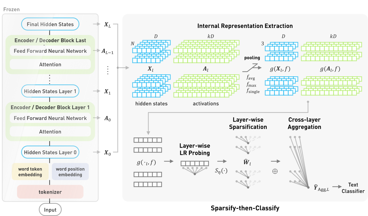
Figure 1: Proposed architecture of Sparsify-then-Classify

3.1 Internal Representation Extraction

In Section 2 we have described how the last layer of hidden state records are condensed token-wise by the pooling function extracting the result on the specific position at a certain single token, which is purely based on the way the model is pretrained on the last layer of output, ignoring the large amount of potentially useful information inside the sentence and model. Previous studies (Bills et al., 2023) have shown that the activations among tokens within the sentence input also hold meaningful position-specific patterns that vary across different layers of the model, intuitively suggesting more expressive representations to be utilized.

Hence in this study, we investigate the FFN activations and hidden states for all layers

$$g(\bm{X}_{l},f_{\text{single}}:\mathbb{R}^{N}\mapsto\mathbb{R}) :\mathbb{R}^{N\times D}\mapsto\mathbb{R}^{D}\qquad l=0,\cdots,L$$

$$g(\bm{A}_{l},f_{\text{single}}:\mathbb{R}^{N}\mapsto\mathbb{R}) :\mathbb{R}^{N\times A}\mapsto\mathbb{R}^{A}\qquad l=0,\cdots,L-1$$

along with two more pooling methods, average pooling and max pooling, to additionally express more detailed information about how specific neurons are activated across tokens within a sentence.

By using $f\in\{f_{\text{avg}},f_{\text{max}},f_{\text{single}}\}$ we map the hidden states and activation of sentences with variable lengths into a feature space with a static size of $3$. The pooled hidden states $\{g(\bm{X},f_{\text{avg}}),g(\bm{X},f_{\text{max}}),g(\bm{X},f_{\text{single}})\}$ and activations $\{g(\bm{A},f_{\text{avg}}),g(\bm{A},f_{\text{max}}),g(\bm{A},f_{\text{single}})\}$ are calculated in batches and stored.

3.2 Linear Probing

On the existing understanding of the LLM interpretability literature, it is important to note the linear representation hypothesis, which posits that features within neural networks are represented linearly (Mikolov et al., 2013, Elhage et al., 2022). By delving deeper into these linear dimensions, linear probing (Alain and Bengio, 2016) could help unravel the intricate functionalities of LLM internal representations. Therefore our investigation focuses on the technique of linear probing on each layer independently within LLM internal representations, which is widely adopted for interpretability and evaluating the quality of features in LLMs (Dalvi et al., 2019, Suau et al., 2020, Wang et al., 2022, Gurnee et al., 2023).

Based on the pooled results of hidden states and FFN activations, we train logistic regressors (LR) with $\mathcal{L}^{1}$-regularization (also known as Lasso regularization) as the linear classifier probes, to predict the category that the text belongs to. Each layer of the LLMs is examined independently to understand the behavior and contribution of neurons at different depths. For LR probes, the objective is to predict the target $\bm{Y}\in\mathbb{R}^{B}$ from pooled hidden states $g(\bm{\tilde{X}}_{l},f)\in\mathbb{R}^{B\times D}$ or activations $g(\bm{\tilde{A}}_{l},f)\in\mathbb{R}^{B\times(kD)}$ for all $B$ sentences at a given layer $l$ of model. The optimization problem for fitting LR probes with $\mathcal{L}^{1}$-regularization is formulated as:

$$\bm{\hat{W}}_{X,l},\bm{\hat{b}}_{X,l} =\arg\min_{\bm{W},\bm{b}}||\bm{Y}-\sigma(g(\bm{\tilde{X}}_{l},f)\bm{W}+\bm{b})||_{1}+\lambda||\bm{W}||_{1},\qquad l=0,\cdots,L$$

$$\bm{\hat{W}}_{A,l},\bm{\hat{b}}_{A,l} =\arg\min_{\bm{W},\bm{b}}||\bm{Y}-\sigma(g(\bm{\tilde{A}}_{l},f)\bm{W}+\bm{b})||_{1}+\lambda||\bm{W}||_{1},\qquad l=0,\cdots,L-1$$

where $\sigma(\cdot)$ denotes the logistic sigmoid function, and $\lambda\geq 0$ is the regularization parameter that controls the trade-off between the fidelity of the model to the training data and the complexity of the model’s weights. The term $||\bm{W}||_{1}$ represents the $\mathcal{L}^{1}$-norm of the weight vector, which is the sum of the absolute values of the weights. The regularization term controlled by hyper-parameter $\lambda$, encourages sparsity in the weight vector, effectively performing feature selection by driving certain weights to zero. The regression yields a logistic predictor $\bm{\hat{Y}}_{X}=\sigma(g(\bm{\tilde{X}}_{l},f)\bm{\hat{W}}_{X,l}+\bm{\hat{b}}_{X,l})$ and $\bm{\hat{Y}}_{A}=\sigma(g(\bm{\tilde{A}}_{l},f)\bm{\hat{W}}_{A,l}+\bm{\hat{b}}_{A,l})$ of each layer for inference.

3.3 Layer-wise Sparsification

One aspect of the $\mathcal{L}^{1}$-regularized LR probes is that the learned weights $\bm{\hat{W}}$ can be interpreted as indicators of the importance of neurons at that layer for the specific task (Tibshirani, 1996, Ng, 2004). Weights with higher magnitudes suggest that the corresponding neurons play a crucial role in making task-specific predictions. When a weight is close to zero, it indicates that the corresponding contribution of the neuron is minute for the task. In essence, LR probes provide a mechanism to identify task-specific salient neurons within the internal representations of LLMs. By the sparsity of $\mathcal{L}^{1}$-regularized LR weights, where weights have been inherently pushed towards zero with less important features often having weights exactly at zero, we can derive an intuitive criterion for neuron selection.

Here we consider the trained LR probes as sparsified salient feature indicators by investigating the magnitude of weights they learned. Given logistic predictor $\bm{\hat{Y}}_{X}=\sigma(g(\bm{\tilde{X}}_{l},f)\bm{\hat{W}}_{X,l}+\bm{\hat{b}}_{X,l})$ and $\bm{\hat{Y}}_{A}=\sigma(g(\bm{\tilde{A}}_{l},f)\bm{\hat{W}}_{A,l}+\bm{\hat{b}}_{A,l})$ for each layer $l=0,\cdots,L_{\text{temp}}$ as the LR probes we trained independently based on each layer’s hidden states and activations by running the LLM up to layer $L_{\text{temp}}$, we focus on the logistic regression weights $\bm{\hat{W}}_{X,l}\in\mathbb{R}^{D}$ and $\bm{\hat{W}}_{A,l}\in\mathbb{R}^{(kD)}$.

In this context a measure that emphasizes larger weights is advantageous, as it aligns with the underlying assumption that a higher logistic regression weight correlates with stronger informativeness and a more significant contribution the corresponding input feature makes to the model’s predictive capacity. Consequently, ranking neurons according to their absolute magnitude of weights in trained linear probes yields good feature selection results in LLMs (Bau et al., 2018, Dalvi et al., 2019). At the same time, selecting a large number of features, especially those that are not strongly predictive of the outcome, will dilute the effect of the predictive features and make it harder to identify the signal amidst the noise (Guyon and Elisseeff, 2003).

To encourage better layer-wise sparsification, we introduce the squared $\mathcal{L}^{2}$-norm from the perspective of signal processing to being employed as a measure of the energy exerted by the LR weights. Mathematically, the squared $\mathcal{L}^{2}$-norm of a weight vector $||\bm{\hat{W}}||_{2}^{2}$ as the sum of the squares of its components, effectively amplifies the impact of larger weights, thereby providing a unified scale that accentuates the more influential features in terms of their contribution to the model’s predictions (Hastie et al., 2009). On this foundation, a threshold $\eta$ is established on the squared $\mathcal{L}^{2}$-norm $||\bm{\hat{W}}_{X,l}||_{2}^{2}$ and $||\bm{\hat{W}}_{A,l}||_{2}^{2}$, which is calculated by the sum of squared weights corresponding all input features within that layer, serving as a measure of the cumulative importance of different features’ contributions to the layer’s LR probe. By sorting all squared feature weights in descending order and calculating the cumulative sum across features, we can assess the collective importance of any given set of individual features. when the cumulative sum for a set of neurons $S_{\eta}(\bm{\tilde{X}}_{l})$ or $S_{\eta}(\bm{\tilde{A}}_{l})$ exactly exceeds $\eta||\bm{\hat{W}}_{X,l}||_{2}^{2}$ for hidden states or $\eta||\bm{\hat{W}}_{A,l}||_{2}^{2}$ for activation, we designate the given set of neurons as salient. This process, similar to the weight pruning techniques in neural networks (LeCun et al., 1989) that adopts backward elimination of variables, can effectively filter out neurons with minimal impact according to the learned logistic regression weights, thereby emphasizing the features most relevant to the probe’s decision-making.

3.4 Cross-layer Aggregation

Current probing techniques predominantly focus on layer-specific analysis that falls short in detecting features distributed across multiple layers of the model (Gurnee et al., 2023). A straightforward concatenation of all layer inputs is not a viable solution; such an approach suffers from the nature of sparsity of LLM internal representations, rendering training process ineffective. A common understanding in the field of interpretation, particularly studies on generative models, suggests a potential solution. In LLMs it is often observed that the lower layers tend to focus on encoding elementary features of input text like syntax, grammar, and basic semantics, foundational information which higher layers utilize for more abstract and complex aspects of understanding broader concepts, generating coherent responses, applying more sophisticated operations like deduction and creativity, etc. (Dalvi et al., 2022, Sajjad et al., 2022, Wang et al., 2022, Voita et al., 2023)

To address this, we introduce a simple yet highly potent way to aggregate the salient neurons dispersed across various layers together, using previously attributed layer-specific importance of hidden state and activation features. The neurons passing the $\eta$ criterion are now leveraged to construct a refined feature vector record for each instance, aggregating across the collected layers to highlight the features learned at different parts of LLM. The rationale behind this aggregation is to harness the diverse yet complementary information captured by different layers of the LLM, thereby enhancing the overall predictive capability on specific text classification tasks. This aggregation forms a composite representation $\bm{\tilde{X}}_{\text{Agg},L_{\text{temp}}}$ and $\bm{\tilde{A}}_{\text{Agg},L_{\text{temp}}}$, by concatenating the activations and hidden states of selected salient neurons from the previous layer-wise sparsification process:

$$\bm{\tilde{X}}_{\text{Agg},L_{\text{temp}}} =\bigoplus_{l=0}^{L_{temp}}\bigoplus_{i\in{S_{\eta}(\bm{\tilde{X}}_{l})}}\bm{\tilde{X}}_{l,i},\qquad L_{\text{temp}}=0,\cdots,L$$

$$\bm{\tilde{A}}_{\text{Agg},L_{\text{temp}}} =\bigoplus_{l=0}^{L_{temp}}\bigoplus_{j\in{S_{\eta}(\bm{\tilde{A}}_{l})}}\bm{\tilde{A}}_{l,j},\qquad L_{\text{temp}}=0,\cdots,L-1$$

where $\bigoplus$ represents concatenation, $S_{X,l}$ and $S_{A,l}$ the sets of indices for salient neurons in hidden states and activations, respectively, and $\bm{\tilde{X}}_{l,i}$ and $\bm{\tilde{A}}_{l,j}$ the hidden states and activations at the $i$-th and $j$-th salient feature in layer $l$ of model.

Finally, we utilize these aggregated feature vectors to train higher-order LR classifiers for each $L_{\text{temp}}$ on pooled representations $g(\bm{\tilde{X}}_{\text{Agg},L_{\text{temp}}},f)$ and $g(\bm{\tilde{A}}_{\text{Agg},L_{\text{temp}}},f)$, which yields logistic predictors $\bm{\hat{Y}}_{\text{Agg},X,L\text{temp}}=\sigma(g(\bm{\tilde{X}}_{\text{Agg},L_{\text{temp}}},f)\bm{\hat{W}}_{X,L_{\text{temp}}}+\bm{\hat{b}}_{X,L_{\text{temp}}})$ and $\bm{\hat{Y}}_{\text{Agg},A,L\text{temp}}=\sigma(g(\bm{\tilde{A}}_{\text{Agg},L_{\text{temp}}},f)\bm{\hat{W}}_{A,L_{\text{temp}}}+\bm{\hat{b}}_{A,L_{\text{temp}}})$ for each $L_{\text{temp}}$, as our text classifiers.

To summarize, we present the overall algorithm design of STC within 3.2, 3.3 and 3.4 as an end-to-end solution for leveraging the internal representations of LLMs for text classification tasks, as illustrated in Algorithm 1.

Input: $\{g(\bm{\tilde{A}}_{l},f),\quad l\in\{0,\cdots,L_{\text{temp}}-1\}\},\bm{Y},\eta\in(0,1)$

Output: $\bm{\hat{Y}}_{\text{Agg}}=\sigma(g(\bm{\tilde{A}}_{\text{Agg}},f)\bm{\hat{W}}+\bm{\hat{b}}),\hat{l}_{\text{Agg}}$

1 $\bm{\tilde{A}}_{\text{Agg}}\leftarrow\varnothing$;

2 $\bm{\hat{Y}}_{\text{Agg}}\leftarrow\varnothing$;

3 $\hat{l}_{\text{Agg}}\leftarrow 0$;

4 $l\leftarrow 0$;

5 while $l<L_{\text{temp}}$ do

       /* Layer-wise LR Probing */

6       $\bm{\hat{W}},\bm{\hat{b}}\leftarrow\arg\min_{\bm{W},\bm{b}}||\bm{Y}-\sigma(g(\bm{\tilde{A}}_{l},f)\bm{W}+\bm{b})||_{1}+\lambda||\bm{W}||_{1}$;

       /* Layer-wise Sparsification */

7       $\bm{J}\leftarrow$ index$(\bm{\hat{W}})$;

8       $\bm{\hat{W}},\bm{J}\leftarrow$ sort$(\bm{\hat{W}},\bm{J})$;

9       $\bm{S}\leftarrow\varnothing$;

10       $\Sigma\leftarrow 0$;

11       $k\leftarrow 1$;

12       while $\Sigma\leq\eta\cdot||\bm{\hat{W}}||_{2}^{2}$ do

13             $\bm{S}\leftarrow\bm{S}\cup\{\bm{J}_{k}\}$;

14             $\Sigma\leftarrow\Sigma+(\bm{\hat{W}}_{k})^{2}$;

15             $k\leftarrow k+1$;

16            

      /* Cross-layer Aggregation */

17       $\bm{\tilde{A}}_{\text{Agg}}\leftarrow\bm{\tilde{A}}_{\text{Agg}}\cup\{\bm{\tilde{A}}_{l,i}\forall i\in\bm{S}\}$;

18      

19      $\bm{\hat{W}},\bm{\hat{b}}\leftarrow\arg\min_{\bm{W},\bm{b}}||\bm{Y}-\sigma(g(\bm{\tilde{A}}_{\text{Agg}},f)\bm{W}+\bm{b})||_{1}+\lambda||\bm{W}||_{1}$;

20      

21      $\bm{\hat{Y}}=\sigma(g(\bm{\tilde{A}}_{\text{Agg}},f)\bm{\hat{W}}+\bm{\hat{b}})$;

22       if $||\bm{Y}-\bm{\hat{Y}}||_{1}<||\bm{Y}-\bm{\hat{Y}}_{\text{Agg}}||_{1}$ then

23             $\bm{\hat{Y}}_{\text{Agg}}\leftarrow\bm{\hat{Y}}$;

24             $\hat{l}_{\text{Agg}}\leftarrow l$;

25            

26      

Algorithm 1 Sparsify then Classify

4 Experimental Setup and Results

4.1 Data Ingredients Preparation

To evaluate the performance of STC leveraging the internal representations of LLMs as text classifiers, we collect 3 relevant datasets and study the hidden states and FFN activation patterns of multiple well-established transformer-based language models: RoBERTa, DistilBERT, and GPT2 family, including GPT2, GPT2-M, GPT2-L and GPT2-XL.

Dataset Collection

We select the following 3 datasets, as details summarized in Table 3:

• IMDb: The IMDb dataset (Maas et al., 2011) is one of the most popular sentiment classification datasets, curated for the binary classification task of positive and negative movie reviews.

• SST-2: The SST-2 dataset for sentiment analysis, part of the General Language Understanding Evaluation (GLUE) benchmark (Wang et al., 2018), provides a binary classification task based on the Stanford Sentiment Treebank. The true test set labels of datasets within GLUE benchmark are not publicly accessible, and conventionally the fine-tuned models often report the performance on the validation set, hence we adopt the same approach by using the original validation set as the test set.

• EDOS (SemEval-2023 Task 10): Kirk et al. (2023) collects dataset for facilitating exploratory experiments of Explainable Detection of Online Sexism (EDOS). The dataset contributes a hierarchical taxonomy of sexism content, in which we select Task A for our experiments, where systems are expected to predict whether a post is sexist or not.

Table 3: All datasets and features used

Dataset	Subset	Task	Class	# of Text
IMDb	—	Sentiment Analysis	pos, neg	50,000
GLUE	sst2	Sentiment Analysis	pos, neg	70,000
EDOS	Task A	Stance Detection	non_sexist, sexist	20,000

In practice, if the dataset does not provide a validation set, we randomly split 20% of the training set as validation and record the random seed to ensure reproducible results.

Inner Represetation Acquisition

We replicated and validated the forward pass of DistilBERT, RoBERTa base, GPT2 base, GPT2-M, GPT2-L, and GPT2-XL model to access their internal representations, integrating with both pretrained and fine-tuned weights sourced from HuggingFace. Within each transformer block in the models, the activations of the Feed-Forward Neural Network, which comprises $A=kD$ neurons in each transformer block, along with block hidden states comprising $D$ neurons in between transformer blocks, are collected, pooled using $f\in\{f_{\text{avg}},f_{\text{max}},f_{\text{single}}\}$, and stored.

4.2 Baseline Performance

Sentence Embedding

For BERT and its variants, the models take the output of [CLS] token in the final hidden states for downstream tasks (Devlin et al., 2018). For the GPT2 family, models take the final hidden states output of the last valid token for each input sequence to perform downstream tasks. Thus, We collect the output of the first [CLS] token in the last layer hidden states for BERT and its variants, and output of the last valid tokens for each sentence in the last layer hidden states from GPT2 and its variants. A fully connected layer with softmax is then trained atop with $\bm{\tilde{Y}}=\text{softmax}(g(\bm{\tilde{X}}_{L},f_{\text{single}})\bm{W})$. The results are calculated in our experiments and presented in the Embedding column of Table 4 as the frozen LLM baseline performance.

Model Fine-tuning

For all the fine-tuned models we found that were fine-tuned on the studied dataset and uploaded to HuggingFace, we test their baseline performance using the same classification head structure as the sentence embedding approach, and compare the results with those reported on the corresponding model web pages. Several notable findings comparing our experiment results to the reported ones are discussed in 5.1.2. The results are reported in the Fine-tuning column of Table 4 as the baseline performance of fine-tuned LLMs, in which the entries for several models are skipped as no publicly available fine-tuning models.

In-context Learning

The in-context learning (ICL) approach, particularly fashionable in the realm triggered by the recent enthusiasm in generative LLMs, involves few-shot learning, i,e, leveraging a limited number of examples within prompts as prefixes and suffixes of input texts to guide the model to generate textual output in the desired way. This technique is provided here as an estimation on the effectiveness of context-based learning without extensive training or fine-tuning, showing the adaptability of pretrained LLMs using a few examples as reference within input for generating response. The results are shown in the ICL avg. column of Table 4, in which entries for BERT variants are skipped as such paradigm is not supported by their encoder-only architecture with no LM heads.

Table 4: Performance of LLM application in text classification for baselines and Sparsify-then-Classify

		Baseline			Frozen + STC		Fine-tuned + STC
Dataset	Model	Embedding	Fine-tuning	ICL avg.	Probes	Agg.	Probes	Agg.
IMDb (acc.)	DistilBERT	86.95	92.80	—	86.34	87.06	92.76	92.88
	RoBERTa	89.61	94.67	—	92.09	92.25	95.64	95.68
	GPT2	85.46	94.06	(55.07)	90.02	90.93	96.05	96.10
	GPT2-M	88.72	(90.70)	(59.48)	92.46	93.37	93.04	93.92
	GPT2-L	91.76	(92.74)	(77.39)	93.22	94.36	93.92	94.76
	GPT2-XL	91.86	(93.11)	(80.43)	94.23	94.92	94.50	95.12
GLUE SST-2 (val acc.)	DistilBERT	84.06	91.30	—	84.06	84.40	90.59	91.19
	RoBERTa	84.06	94.03	—	88.76	90.59	94.15	94.38
	GPT2	85.89	91.51	58.90	85.89	87.73	91.63	92.32
	GPT2-M	86.12	91.98	61.00	87.16	90.25	92.09	92.32
	GPT2-L	90.14	—	74.50	90.94	91.97	—	—
	GPT2-XL	90.02	—	66.80	91.86	93.23	—	—
EDOS Task A (Macro F1)	DistilBERT	65.09	78.74	—	71.16	75.79	80.44	81.12
	RoBERTa	60.29	80.48	—	70.84	73.97	80.32	80.88
	GPT2	68.90	—	(52.97)	72.53	74.19	—	—
	GPT2-M	71.17	—	(55.62)	72.57	75.74	—	—
	GPT2-L	72.05	—	(66.07)	73.44	76.33	—	—
	GPT2-XL	72.56	—	(67.85)	73.88	76.69	—	—

4.3 Sparsify then Classify

Layer-wise Probing

The classification performance of layer-wise linear probes is regarded as an important indicator for measuring the knowledge acquisition in individual layers. To maintain a non-overfitting evaluation of the best per-layer performance, however, it is crucial to note that we treat both the pooling function and the layer l as hyper-parameters. Meanwhile, as the best number of iterations for training the probes cannot be determined in advance, we also treat it as a hyper-parameter with a sufficient maximum limit.

Consequently, the test performance we report is derived from applying this best combination of hyper-parameters, as determined by the validation set, ensuring that our reported results are not overfitted. Our findings are presented in the Probes column of Table 4, demonstrating the fact that the best individual layer performance of both frozen and fine-tuned models could be close to, and mostly even well above the results using their respective classification heads.

In addition, to corroborate the linear representation hypothesis in our selected models and datasets, we also examine the more expressive nonlinear single layer perceptrons (SLP) probes as the comparative group to LR probes. We report the details and results of SLP in A.2.

Feature Sparsification

Once the layer-wise probes are fitted, the weights of the linear models, $\bm{\hat{W}}$, are sorted in descending order, after which the most indicative neurons on the specific task are selected based on their contribution to the model’s predictive power. This selection procedure is achieved by accumulating the squared weights of the neurons until a predefined threshold, $\eta$, of the total squared weight magnitude is reached. The neurons that meet this criterion are then marked as salient for the corresponding layer and prepared for further aggregation. In practice, we have $\eta$ ranged from 0.001 to 0.5, indicating a wide range of levels in sparsification with the number of neurons selected per layer ranging from 1 to 5%-10% of total.

Our experimental results confirm the findings of Wang et al. (2022) and Gurnee et al. (2023) where a minimal amount of most informative neurons could embrace comparable performance with the model classification head, yet within single layer and without further aggregation, we have not found evidence that using only sparsified neurons could yield better performance than than the layer-wise probes. Thus, to visually demonstrate how well feature sparsification actually works, we refer to Section 5.3 with further details showcasing the intrinsic interpretability of STC’s sparsification process.

Multi-layer Aggregation

Finally, the salient neurons identified across different layers of the LLM are combined to form an aggregated representation. This representation is then used to train a new LR model, which is called then-Classify and aligns with our aforementioned linear representation hypothesis. The aggregated LR models, starting from the bottom layer and extending to each subsequent layers, are then evaluated based on their performance in predicting the output categories.

Similar to section 4.3, the processes of evaluating and updating the LR models are all conducted specifically on the validation set . Through this workflow, the predetermined parameters, such as the threshold $\eta$, the choices of pooling methods, and the number of layers to aggregate, are all regarded as hyper-parameters in our reporting the results based on the test performance of the classifier that demonstrates the best performance on the validation set in the Agg. column of Table 4.

Noteworthy Results

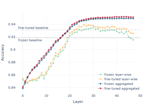
Figure 2: Layer-wise LR probe and aggregated ($\eta=0.5$) performance on IMDb dataset, using max-pooling on GPT2-XL activation records

Here we take the GPT2-XL activation records with max-pooling as a representative example to demonstrate the concrete performance our proposed aggregation method yields. As shown in Figure 2, we report the performance of layer-wise LR probes and cross-layer aggregation with $\eta=0.5$ of each layer for both frozen models and fine-tuned models. In this case, the STC manages to consistently outperform the layer-wise results starting from the second layer (for the first layer only features within $\eta=0.5$ cumulative importance threshold are utilized, thereby leading to a slight decrement in performance). Specifically, during the first half of the model layers the aggregated method yields a smoother rise in the curve above the layer-wise probes, at some point the lift between even approaches 4%. After the layer-wise curve reaches its peak performance and starts to retrace, the aggregation method maintains its performance till the final layer of the model, and even manages to achieve slight improvements from the latter part of the layers.

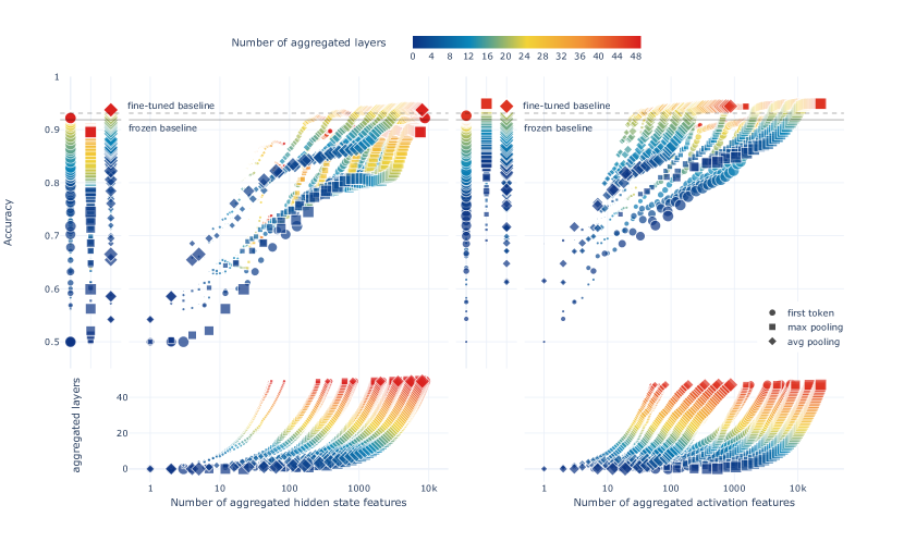
((a))

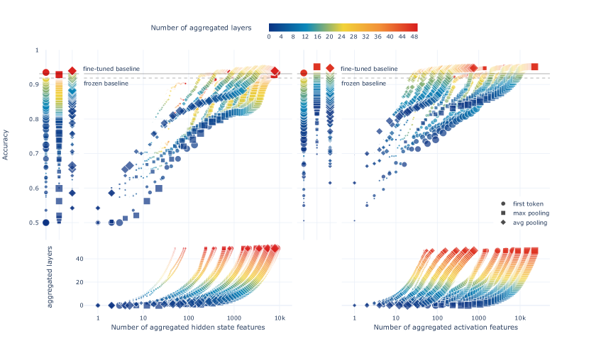
((b))

Figure 3: What-which-where plots for Sparsify-then-Classify performance on frozen and fine-tuned GPT2-XL models over IMDb dataset. The left subfigures are for hidden states, and the right subfigures are for activations.

For a given LLM, we train and evaluate the classifier $\bm{\tilde{Y}}$ on aggregated features for each combination of pooling function $f$, the number of aggregated layers $l$ and the aggregation threshold $\eta$. We refer to Figure 3(a) and Figure 3(b) as what-which-where plots as they visualize the performance along with information of what aggregation threshold is used, which pooling choice is selected, and where in depth the layer aggregation takes place in LLMs. Respectively, the pooling choice is indicated with different marker shapes, the magnitude of $\eta$ is reflected by the marker sizes, and the number of aggregated layers is shown with different colors in the color bar. In addition, we present how the number of features evolves with every combination in the lower subfigures of each plot, further demonstrating the efficacy of STC.

5 Discussion

5.1 Performance

Our experimental evaluations comparing performance metrics of different LLM paradigms along with our approaches yield promising results. Notably, we observed a consistent improvement in performance by integrating our method into well-established approaches, namely comparing the sentence embedding baseline with frozen LLM + STC, and model fine-tuning baseline with fine-tuned LLM + STC in Table 4.

5.1.1 Frozen LLMs

The prevalent practice of sentence embedding in the realm of LLM application involves the employment of frozen models, where the pretrained weights are not modified. This involves appending a task-specific sequence classification head to the top of the model for adapting the pretrained representations to particular tasks. Our experiments suggest that this paradigm exhibits relatively poor performance as expected, and may not fully exploit the model’s capabilities. The limitation primarily lies within the head solely relying on the representation of a single token from the last layer of pretrained models, which, in pretrained models, is originally designed and trained for performing general tasks like token prediction rather than specialized ones. The nuanced, layer-specific representations remain largely untapped, yielding suboptimal task performance.

In contrast, our methodology adopts a more granular approach by delving into the multi-layered architecture of transformer-based LLMs, embarking on an anatomical perspective by exploring the internal representations hidden beneath the final layer outputs. With detailed examination of salient neurons for each layer and layer aggregation strategy capitalizing on the diverse and rich internal features encapsulated across the model’s depth, we manage to harness the previously neglected intermediates. The outcome is a clear elevation in performance, compared with the frozen model’s sentence embedding baseline performance we have a 2.63% (layer-wise) and 3.37% (aggregation) accuracy improvement on average for the IMDb sentiment classification task, demonstrating the effectiveness of the in-depth utilization of LLMs’ inherent capabilities.

5.1.2 Fine-tuned LLMs

Another standard practice undergoes a phase of retraining or fine-tuning massive amounts of pretrained model weights to adapt the head to specific tasks. This process, albeit effective to a certain extent, often demands a significant investment of computational resources and time.

Intriguingly, the experiments on fine-tuned models reveal that our proposed method can always further improve their performance when deployed on already fine-tuned models, with 1.41% (layer-wise) and 1.75% (aggregation) accuracy improvement on average for the IMDb sentiment classification task. This has from another perspective verified our previous testament about the confined informativeness by conventional classification heads’ only using single tokens on the final layer output, and the robustness of our approach that rediscovers the capabilities of inner representation in capturing essential features.

It is also worth mentioning that in our reproducing the reported performance of fine-tuned models, we observed a phenomenon as by freezing the fine-tuned model weights and further retraining the classification head, we could sometimes achieve a higher performance compared with the reported baseline. For example, given reported accuracy results of 92.80%, 94.67%, and 94.06% for fine-tuned DistilBERT, RoBERTa, and GPT2 base models, the corresponding performance of our retrained classification heads are 92.68%, 95.64%, and 95.89%. These originally imperfect fine-tuning classification heads can be attributed to an intrinsic vulnerability of the current fine-tuning strategy, by which the weights of language models along with classification heads on top are jointly evaluated and backward propagated together. Such approach may suffer from the difference in model weight sizes of the LLM and classification head themselves, yielding an inconsistency in the effectiveness of fine-tuning on each part. This becomes more obvious for larger models, where the the pre-trained model and the classification head often require different learning rates for optimal training: the layers having been extensively pre-trained usually only need smaller updates, while the classification head being initialized from scratch, might benefit from larger updates. The discrepancy in the size and complexity between the large pre-trained layers and the relatively small classification head can lead to inefficiencies in joint training. By decoupling the fine-tuned model, our retrained classification heads contribute a better-optimized performance compared with the original ones.

5.1.3 Comparison

Comparing experiments implemented on frozen pretrained models with fine-tuned models, we notice that our approach working on fine-tuned models yields better performance than frozen pretrained ones for each model structure respectively. This not only fits the logic that fine-tuning on LLMs has improved the performance of the classification head’s output as it was originally designed and fine-tuned for, but also suggests that fine-tuning has enhanced the salience of model inner representations in capturing task-specific features as well, which is subsequently leveraged by our method.

Specifically, a pattern could be found that for larger models, the performance improvement that model fine-tuning brings compared with frozen models becomes smaller. For example, for the smallest DistilBERT the accuracy of model fine-tuning is 5.85% higher than the sentence embedding approach, and for GPT2-XL this has dropped to 1.25%. The same can be observed in the results of models integrated with our methods, that the accuracy of fine-tuned + STC is 6.40% higher than frozen + STC for DistilBERT, and only 0.07% higher for GPT2-XL. This suggests a relationship between the size of LLMs and their amenability to fine-tuning, that for larger LLMs, the less improvement introducing model fine-tuning brings. This can be due to the fact that larger pretrained models already hold greater capacity for learning and generalization. Also, the increase in size makes the models harder to be effectively fine-tuned, as with their vast number of parameters, larger models can be more prone to overfitting when fine-tuned on small datasets.

5.2 Efficiency

Efficiency during training and inference in terms of both computational resources and environmental impact have become increasingly relevant in discussions about recent large-scale models and provoked a paramount consideration in the adaptation of LLMs for specialized tasks. Time, storage, money and energy required can often pose significant hurdles, particularly in scenarios with enormous data for training and deployments. In this investigation, we lead a quantitative analysis with trainable parameters, floating-point arithmetic and performance results on the merits of our proposed approach as means to mitigate these challenges, by comparing our method with current fashionable fine-tuning strategies as baseline.

For number of trainable parameters of language models, we report the total amount of trainable parameters within LLM (without embedding layers at the bottom) $N_{\text{param}}$ porvided by HuggingFace. For STC we estimate the number of parameters using

$$N_{\text{param LR}} \approx L(1+k)D$$

$$N_{\text{param STC}} \approx(1+\rho_{\eta}\cdot N_{f}\cdot\frac{L+1}{2})N_{\text{param LR}}$$

where $L$ as the number of layers within LLM, $D$ dimension of LLM hidden states, $k$ the ratio of FFN activation dimension to the hidden states, $\rho_{\eta}$ the ratio of features with $\eta$ parameter selected during aggregation, which we take 0.1 for estimation, and $N_{f}$ the number of pooling methods which we take 3 in our experiments.

For the total floating point operations needed for the conventional practice of model fine-tuning and our STC approach, we estimate with empirical estimations given by (Kaplan et al., 2020), we have

$$C_{\text{LLM train}} \approx 6N_{\text{param}}BS$$

$$C_{\text{LLM forward}} \approx(2N_{\text{param}}+2LND)B$$

in which $B$ represents the batch size, $S$ the steps used in training, $N$ the length of input sequence in tokens. For the cost of layer-wise LR probes and cross-layer aggregation, we can similarly derive

$$C_{\text{LR train}} \approx 2L(1+k)DBS+LBS$$

$$C_{\text{LR forward}} \approx(1+k)DB+B$$

where $k$ the ratio of activation dimension to the hidden states dimension, and

$$C_{\text{Frozen + STC train}} \approx C_{\text{LLM forward}}S+\rho_{\eta}\cdot\frac{L+1}{2}C_{\text{LR train}}$$

$$C_{\text{Frozen + STC forward}} \approx\frac{L_{\text{temp}}}{L}C_{\text{LLM forward}}+C_{\text{LR forward}}\approx\frac{L_{\text{temp}}}{L}C_{\text{LLM forward}}$$

All the training cost here is calculated in terms of $BS$ which is the total amount of input sequences inputted during all epochs in training on the entire training set, and the forward cost is calculated in the amount of input sequences within a single batch.

5.2.1 Training Phase

Our proposed STC method demonstrates a significant reduction in the trainable parameters across all models, as shown in Table 5. For instance, for the largest model GPT2-XL we examined, the STC reduces trainable parameters to just 0.25% of its original amount updated in the standard model fine-tuning baseline.

Table 5: Trainable parameters for fine-tuning baseline and STC

	est. # Trainable Param.
Model	Fine-tuning	STC	est. ratio
DistilBERT	66M	93.3K	707:1
RoBERTa	125M	228K	548:1
GPT2	117M	228K	513:1
GPT2-M	345M	829K	416:1
GPT2-L	774M	1.97M	393:1
GPT2-XL	1.56B	3.97M	393:1

This substantial decrease in complexity not only lessens memory demands particularly when retaining the original pretrained weights, but also accelerates training times in IO especially considering that the fine-tuning approach always updates the whole model in a uniform way even if the forward pass and backward gradient calculations can be parallelized, which is not always feasible. Our approach makes the training process more accessible and feasible, especially in environments with limited hardware computational resources.

Table 6: Training cost on IMDb dataset for fine-tuning baseline and Frozen + STC

	est. total floating point operations
Model	Fine-tuning	Forward	LR Probes	LR Agg.	Frozen + STC	est. Speedup
DistilBERT	9.90T	3.43T	23.0B	8.05B	3.46T	2.86
RoBERTa	37.5T	6.48T	46.1B	30.0B	6.56T	5.72
GPT2	17.6T	6.33T	46.1B	30.0B	6.41T	2.75
GPT2-M	51.8T	18.5T	123B	154B	18.8T	2.76
GPT2-L	116T	41.1T	230B	426B	41.8T	2.78
GPT2-XL	234T	81.8T	384B	941B	83.1T	2.82

In terms of computational load, as measured by floating point operation costs in training shown in Table 6, our STC method consistently shows a reduction across all models. Remarkably, the estimated speedup values range from approximately 2.8 times of traditional fine-tuning methods using all IMDb training data in a single epoch, to an impressive 5.7 times when fine-tuning extends over two epochs, which highlights STC’s significant efficiency advantage.

Intriguingly these benefits of STC appear to be more pronounced in cases where model scales go larger with the same architecture, which is particularly evident when examining results within the GPT2 family. Such a reduction in computational load directly translates to decreased energy consumption and reduced GPU/CPU usage time. Consequently, this leads to enhanced cost-effectiveness, a critical aspect in promoting sustainable AI practices and facilitating large-scale AI deployments.

5.2.2 Inference Phase

Efficiency during inference is crucial for real-time applications and deployments of services that leverage LLMs. The storage needed for storing the model weights and speed at which a model can provide accurate predictions directly impacts the usability and effectiveness of the model in practical scenarios.

Table 7: Performance on IMDb dataset for STC using part of the lower layers of models

		acc. using part (%) of the lower layers
Approach	Model	20%	40%	60%	80%	100%	acc. Baseline
Frozen + STC	DistilBERT	78.37	81.96	83.22	86.64	87.06	86.95
	RoBERTa	86.11	88.35	91.19	92.04	92.25	89.61
	GPT2	85.01	86.85	90.02	90.61	90.93	85.46
	GPT2-M	85.16	87.47	92.18	93.30	93.37	88.72
	GPT2-L	87.48	90.79	93.68	94.25	94.34	91.76
	GPT2-XL	88.66	92.82	94.72	94.88	94.89	91.86
Fine-tuned + STC	DistilBERT	85.36	87.10	90.04	92.00	92.88	92.80
	RoBERTa	85.97	90.62	95.22	95.53	95.68	94.67
	GPT2	89.00	92.07	95.94	95.93	95.95	94.06
	GPT2-M	86.93	90.70	93.45	93.85	93.92	(90.70)
	GPT2-L	87.35	90.91	94.09	94.48	94.76	(92.74)
	GPT2-XL	88.98	92.97	94.87	95.10	95.12	(93.11)

Layer Aggregation

As has already been illustrated in Figure 2, the STC performance is mostly enhanced in the lower half of LLM layers, with only marginal improvements in the rest part of the model. This qualitative observation agrees with our initial idea of introducing layer aggregation as mentioned in 3.4 that the lower layers of LLMs are sufficiently salient for capturing task-specific features within input texts.

Here we further compare the baseline performance of conventional classification heads with our STC method aggregating different proportions of the lower model layers to quantitatively substantiate the possibility of only running part of the LLM forward pass during inference. With our results in Table 7, we can observe that for most cases, utilizing the first 60% layers of the model is sufficient for STC to outperform the corresponding baselines that employ full model forward passes. Based on the results of 20% layers, the incremental improvements for including every additional 20% layers, are on average 3.69%, 3.35%, 0.94%, and 0.23%, among which a clear distinction can be found that highlights the efficiency-performance trade-off.

Such a pattern underscores the effectiveness of our layer aggregation approach. After training and determining an optimal $L_{\text{temp}}$ that balances performance and efficiency as expected, our method can operate efficiently using only initial segments of LLMs, reducing both the storage needs for model weights and the computational time required for inference. This makes the STC a highly pragmatic solution, particularly in efficiency-critical real-world application scenarios that are more speed- and resource-management-focused and less sensitive to performance metrics, such as cases involving handling large volumes of text or API deployments that may face high concurrency demands.

Multi-task Learning

Our approach makes no modification to model weights and hence is inherently suitable for a multi-task learning workflow. This stands in stark contrast to the model fine-tuning approach, which necessitates the training and independent storage of task-specific model weights for each individual task. Once the most compute-intensive acquisition of inner representations from input texts is complete, multiple salient feature sparsification and layer aggregation processes can not only proceed with their training phases respectively focusing on different features for specific tasks in perfect parallel, but are also allowed to generate results in inference at the same time with maintaining the same level of task-specific performance as if they were operating independently. Therefore, in cases where multiple tasks are present, our STC approach showcases a significant advantage over model fine-tuning by achieving multiple times savings in model weight storage as reported in Table 5 of trainable parameters, speedups in training floating point operation costs as in Table 6 and in inference as in Table 7.

5.3 Intrinsic Interpretability

The interpretability of machine learning models, especially LLMs that have often been criticized as “black box" models, is always crucial for researchers to understand how these models make decisions, and can also become an essential aspect for transparency-demanding real-world applications. In this section, we focus on providing a brief illustration and discussion on the interpretability of our STC method.

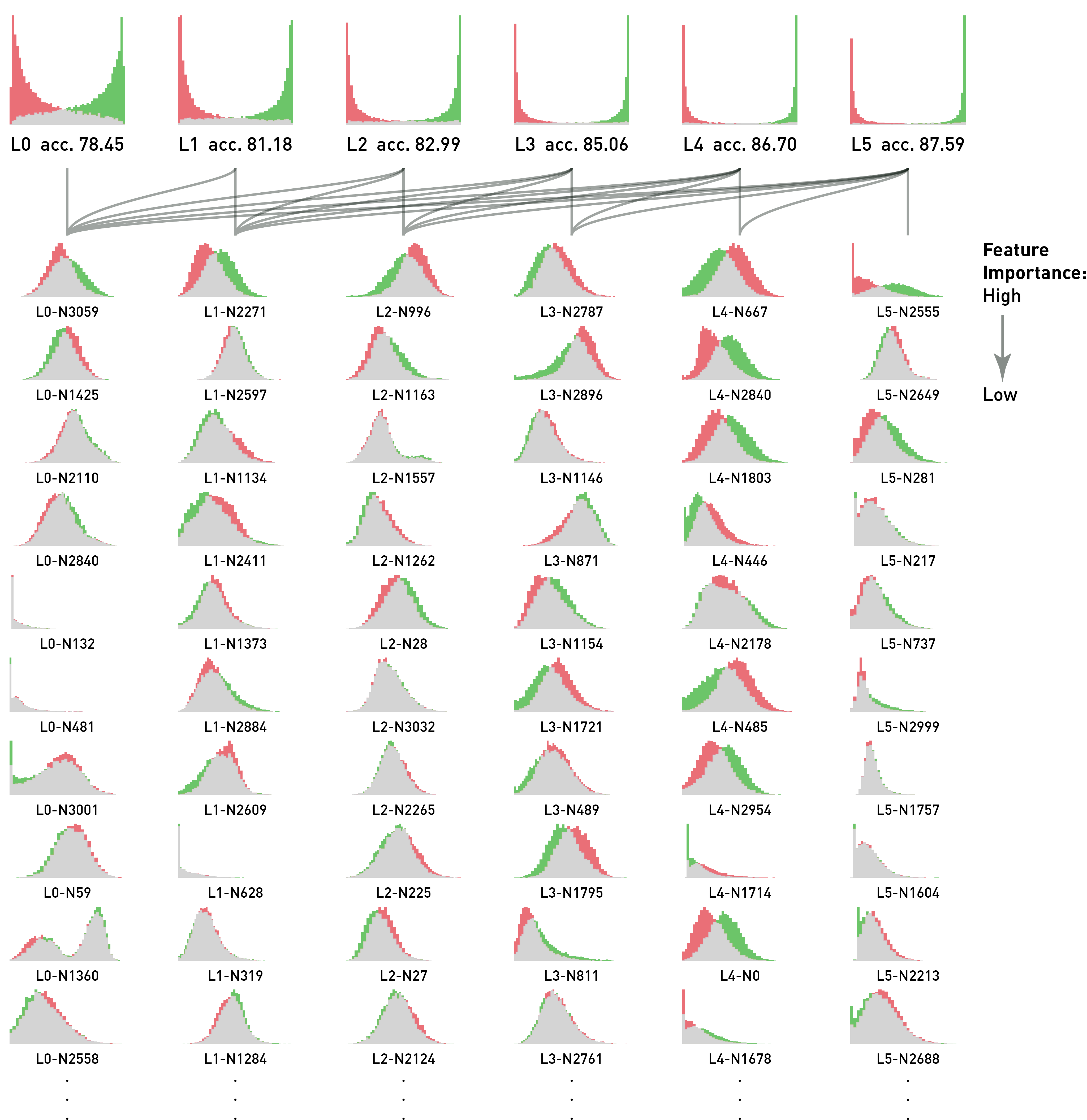
((a)) Layer-wise sparsification and cross-layer aggregation results

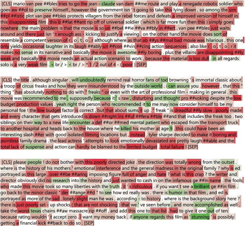
(b1) negative samples

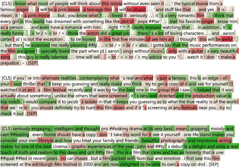
(b2) positive samples

((b)) Token-wise classification results

Figure 4: DistilBert Frozen + STC on IMDb dataset, with $\eta=0.4$ and max pooling on activation records

Sparisifed Neurons vs. Aggregated Classifiers

Here we illustrate how STC gains its ability by its layer-wise feature sparsification and cross-layer aggregation processes. In Figure 4(a) we plot the histograms of the sparsified neuron activations in each layer in a descending way of their importance attributed by layer-wise probing, along with the aggregated STC prediction results, by which we use the sigmoid function output the logistic predictor $\bm{\hat{Y}}_{\text{Agg},A,L\text{temp}}=\sigma(g(\bm{\tilde{A}}_{\text{Agg},L_{\text{temp}}},f)\bm{\hat{W}}_{A,L_{\text{temp}}}+\bm{\hat{b}}_{A,L_{\text{temp}}})$ for each $L_{\text{temp}}$ yields.

As is illustrated in the upper part of Figure 4(a), each layer of the sparsified neurons collectively contributes their distinctiveness of positive and negative samples to the aggregated classifiers at that layer and above, consistently resulting in better performance of the aggregated classifiers at higher levels. This visualization helps in understanding how neurons and layers with different levels of abstraction in the model empower the overall decision-making and performance of the aggregation process for text classification tasks.

As mentioned in 3.3, our layer-wise sparsification is actually a greedy strategy that approximates a 1-step backward elimination process which efficiently filters out the least promising features, yet for getting an exact ranking of features requires a progressively multi-step filtering techniques (LeCun et al., 1989, Dalvi et al., 2019), which is less favorable in our case as another cross-layer aggregation structure would be trained above the filtered sparsification results. When examining individual neurons in each layer, the abilities of their activations in separating samples apart are indeed not strictly in the order of their importance attributed by layer-wise LR probes, as they adopt a linear combination perspective instead of naïvely estimating each neuron’s contribution independently. In LLMs, there are often scenarios where individual neuron activations might not be significantly indicative of studied classification labels on their own, but when combined, reveal a clearer picture, for instance, the contextual polarities, intensity modifiers, sarcastic statements, etc. Features that seem useless by themselves can provide performance improvement when taken together with others (Guyon and Elisseeff, 2003), this nature allows our retraining of LR in cross-layer aggregation to further capture the nuances within selected features, which can been verified by comparing the layer-wise and aggregated performance results in Figure 2 as well.

Generalization to Token-level Classification

Extending the trained sentence-wise classifiers to provide token-wise predictions provides a transparent breakdown of how each token contributes to the sentence-level classification, allows for a nuanced post-hoc examination of understanding of how STC processes and interprets each individual components (words or sub-word patterns) of the input text, and also serve as a proof showcasing the robustness of cross-domain generalization adaptability of our method. This can be implemented as a tool for real-world applications in visualizing complex sentences or documents where different parts may carry different classification results, laying the foundation for more transparent, accountable, and user-trustworthy systems.

By examining Figure 4(b), it is evident that the STC prediction results correspond well with the fine-grained local sentiment expressed by individual tokens at different places within both positive and negative sample sentences. This remarkable capabilities come from incorporating the max and average pooling strategies in our approach, which enable the model initially trained on more generalized features to adeptly transition to recognizing token-specific patterns. In contrast, baseline models typically lack this nuanced capability of transferring to a token-level breakdown since they are largely constrained by their structural dependencies on the first or last token results for performing classification.

6 Related Work

Conventional LLM Application Paradigms in Text Classification

In the realm of text classification, LLMs are applied through distinct paradigms, each with unique methodologies and focal areas. Traditional paradigms include the following three: sentence embedding method, model fine-tuning, and in-context learning. The sentence embedding approach, following Mikolov et al. (2013), primarily utilizing encoder-focused LLMs, leverages the last layer’s hidden states of single tokens, focusing on generating sentence-level embeddings for text classification without modifying model weights or prompt fine-tuning, as demonstrated in seminal works by Le and Mikolov (2014), Devlin et al. (2018), Reimers and Gurevych (2019), etc. In contrast, the model fine-tuning approach involves a comprehensive adaptation of the entire LLM structure, including model weights and classification heads, for task-specific adjustments, with research including Howard and Ruder (2018), Sun et al. (2019) and Yu et al. (2019) demonstrating the effectiveness. The in-context learning (ICL) approach, exemplified by a trend of generative models after GPT-3 (Brown et al. (2020)), adopts a decoder-focused structure and relies on prompt-based learning without altering model weights or using a separate classification head, offering a flexible and prompt-driven methodology.

Interpreting Internal Representations

The quest to unravel the interpretability of model internal representations has long become a cornerstone in understanding AI decision-making process. Classic methods like word2vec (Mikolov et al., 2013) initially illustrated that linearly interpretable features capturing semantic nuances could be extracted from embedding spaces. Alain and Bengio (2016) introduced the concept of linear probes for deep convolutional networks. Subsequent research in LLMs has furthered our understanding in how they acquire task-specific knowledge, including studies by Geva et al. (2020) delving into how FFN layers in transformer-based models operate as key-value memories, Dai et al. (2021) exploring the concept of knowledge neurons within Transformer models, and Suau et al. (2020) identifying specific LLM units as experts in certain aspects of tasks based on their pattern of activations. Burns et al. (2022) and Gurnee and Tegmark (2023) have explored the encoding of spatial, temporal, and factual data within LLMs. Recent work by OpenAI including Bills et al. (2023) extends our understanding of LLMs by letting GPT4 to interpret the different levels of features captured by individual neurons in GPT2-XL. This collection of research has provided vast evidence of internal representations in LLMs being able to capture task-specific features.

Leveraging Internal Representations as Text Classifiers

Leveraging activations and hidden states of LLMs for text classification tasks has gained traction. Studies as early as Radford et al. (2017) have shown the potential of utilizing individual neuron activations in LSTM to conduct sentiment classification. Research by Durrani et al. (2020) and Gurnee et al. (2023) provided further insights into hidden states being used for linguistic and factual representation in models like ELMo, BERT, and the Pythia family. Closely relevant research also includes Wang et al. (2022) identifying specific neurons within RoBERTa that are responsible for particular skills over neuron activations, and empirically validating the potential of using the top-ranked task-specific neurons for classification with competitive performance. Moreover, Durrani et al. (2022) and Gurnee and Tegmark (2023) from the LLaMA2 family, demonstrated the effectiveness of leveraging these internal representations for more nuanced and specific text classification tasks. These works highlight the adaptability and robustness of LLMs in text classification by employing innovative techniques like sparse probing to unravel the complexities within the internal representations, and herald the potential for better text classifiers using neuron representations than LM head or classification head.

7 Conclusion

In this work, we introduce a novel approach, Sparsify-then-Classify (STC), for leveraging the internal representations of Large Language Models (LLMs) in text classification tasks. Our methodology diverges from traditional practices, such as sentence embedding and model fine-tuning, by focusing on the rich, yet often neglected, intermediate representations within LLMs. We demonstrate that by utilizing multiple pooling strategies and layer-wise linear probing to identify salient neurons and aggregating these features across layers, we can significantly boost the performance and efficiency of LLMs as text classifiers.

The experimental results across various datasets and LLM architectures, including RoBERTa, DistilBERT, and the GPT2 family, empirically highlight the effectiveness of our approach. Notably, the STC method consistently outperforms traditional sentence embedding approaches when applied to frozen models and even improved the performance of already fine-tuned models. This enhancement is particularly evident in larger models, where our method effectively leveraged the complex, multi-layered structure of LLMs.

In terms of efficiency, the STC approach shows substantial reductions in the number of trainable parameters and computational load during the training phase, and versatility of efficiently utilizing the lower layers of LLMs and multi-task learning strategies in inference phases. This efficiency gain is crucial, considering the growing concerns about the environmental and computational costs associated with training and deploying large-scale models.

Additionally, by visualizing a breakdown of the intrinsic sparisification and aggregation processes and the token-level classification possibilities, we underscore the advanced interpretability and adaptability of STC in handling complex textual nuances.

Future Work

Looking ahead, there are several promising directions for further refining and extending our methodology. By exploring these avenues, we envision a comprehensive enhancement of the understanding and utilization of LLMs, making them more efficient, interpretable, and adaptable to a wide range of applications.

• Advanced Layer Aggregation Techniques The current approach of layer aggregation in STC is relatively simplistic and intuitive. Future work could explore more advanced methods for aggregating features sparsified across layers, potentially using learning techniques to automatically determine the most effective combination of layers and features for a given task.

• Adaptation to Other NLP Tasks While this study focused on text classification, the STC method has potential applications in other NLP tasks such as regression and token-level classification. Adapting and optimizing STC for these tasks could further demonstrate its versatility.

• Incorporation of Unsupervised Learning Leveraging unsupervised or semi-supervised learning techniques in the STC framework could allow it to automatically discover features and attribute them accordingly, enhancing its applicability in scenarios with limited labeled data. This could make the approach more accessible and reduce the reliance on extensive labeled datasets.

• Exploration of Transfer Learning Investigating the transferability of our approach across different domains could be valuable. Understanding how well the salient features identified in one domain can be adapted to another could lead to more efficient model training and broader applicability.

Appendices

Appendix A.1 Baseline Architecture

Figure 5 illustrates the detailed architectures for text classification using LLMs in three conventional mainstream paradigms, which are served as baseline methods in our study.

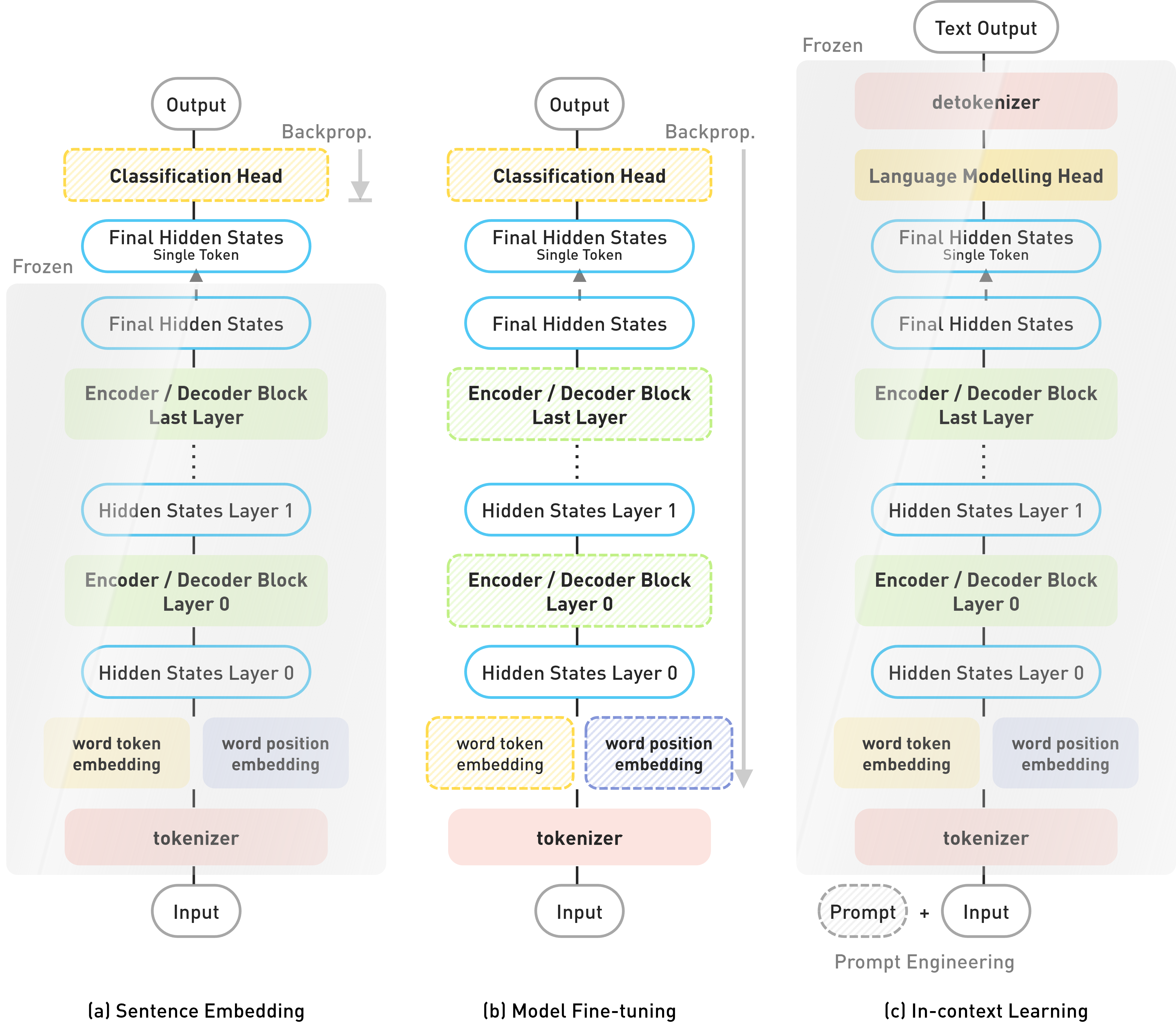
Figure 5: Baseline architectures for LLM application in text classification

Appendix A.2 Linear vs. Nonlinear Probes

In addition to linear probes, we examine the Single Layer Perceptron as nonlinear probes with $S_{X}=\sqrt{D}$ neurons in its mere hidden layer for probing hidden state representations, and $S_{A}=\sqrt{kD}$ neurons for probing FFN activations. This is to decode the potential non-linearity of LLM internal representations, such as polysemantic properties, by introducing a substantially more expressive model. The optimization of SLP probes can be formulated as

$$\bm{\hat{W}}_{X,l},\bm{\hat{b}}_{X,l} =\arg\min_{\bm{W},\bm{b}}||\bm{Y}-\sigma((f_{\text{act}}(g(\bm{\tilde{X}}_{l},f)\bm{W}_{1}+\bm{b}_{1})\bm{W}_{2}+\bm{b}_{2}))||_{1},\qquad l=0,\cdots,L$$

$$\bm{\hat{W}}_{A,l},\bm{\hat{b}}_{A,l} =\arg\min_{\bm{W},\bm{b}}||\bm{Y}-\sigma((f_{\text{act}}(g(\bm{\tilde{A}}_{l},f)\bm{W}_{1}+\bm{b}_{1})\bm{W}_{2}+\bm{b}_{2}))||_{1},\qquad l=0,\cdots,L-1$$

Table 8: Performance on IMDb dataset for LR and SLP probes on individual layers of frozen LLMs

		Pooled Activations from Single Layer
Model	Baseline	0	2	4	6	8	10	12	16	20	25	32	last
DistilBERT + Linear	86.95	82.85	84.06	87.24	—	—	—	—	—	—	—	—	86.12
DistilBERT + SLP	87.37	85.83	86.68	88.53	—	—	—	—	—	—	—	—	88.25
RoBERTa + Linear	89.61	83.54	86.31	89.65	92.09	90.99	90.65	—	—	—	—	—	90.18
RoBERTa + SLP	91.11	86.51	88.84	91.22	93.18	92.72	92.49	—	—	—	—	—	91.39
GPT2 + Linear	85.46	85.04	83.92	86.72	89.46	90.12	89.85	—	—	—	—	—	89.30
GPT2 + SLP	86.78	87.03	87.08	89.07	91.27	91.25	90.80	—	—	—	—	—	89.66
GPT2-M + Linear	88.72	85.80	84.03	84.59	86.50	89.18	90.77	91.83	92.51	91.74	—	—	91.45
GPT2-M + SLP	89.82	87.41	86.74	87.69	89.36	90.87	92.23	92.85	92.77	92.32	—	—	91.57
GPT2-L + Linear	91.76	84.94	83.46	84.23	84.67	85.36	87.05	88.25	92.00	93.13	93.21	92.69	92.06
GPT2-L + SLP	90.59	87.57	87.34	87.52	88.26	88.54	89.92	90.32	92.67	93.74	93.44	92.07	91.92
GPT2-XL + Linear	91.86	85.47	84.74	85.09	85.15	85.96	87.07	88.44	90.47	93.11	93.92	93.82	93.10
GPT2-XL + SLP	91.32	87.22	86.81	87.84	88.49	88.33	89.67	91.09	92.29	93.50	93.69	93.56	92.35

For $f_{\text{act}}$ we used ReLU as the activation function in our SLP probes. We report the testing accuracy of IMDb dataset for both sequence classification head and layer-wise probing in Table 8, demonstrating that the more expressive SLP yields a minute and inconsistent improvement for all models. The results are referred to as decent support to the hypothesis that for the text classification tasks, the features are as well represented linearly in Large Language Models.

References

- Alain and Bengio (2016) Guillaume Alain and Yoshua Bengio. Understanding intermediate layers using linear classifier probes. arXiv preprint arXiv:1610.01644, 2016.
- Bau et al. (2018) Anthony Bau, Yonatan Belinkov, Hassan Sajjad, Nadir Durrani, Fahim Dalvi, and James Glass. Identifying and controlling important neurons in neural machine translation. arXiv preprint arXiv:1811.01157, 2018.
- Bills et al. (2023) Steven Bills, Nick Cammarata, Dan Mossing, Henk Tillman, Leo Gao, Gabriel Goh, Ilya Sutskever, Jan Leike, Jeff Wu, and William Saunders. Language models can explain neurons in language models. URL https://openaipublic.blob.core.windows.net/neuron-explainer/paper/index.html. (Date accessed: 14.05. 2023), 2023.
- Brown et al. (2020) Tom Brown, Benjamin Mann, Nick Ryder, Melanie Subbiah, Jared D Kaplan, Prafulla Dhariwal, Arvind Neelakantan, Pranav Shyam, Girish Sastry, Amanda Askell, et al. Language models are few-shot learners. Advances in neural information processing systems, 33:1877–1901, 2020.
- Burns et al. (2022) Collin Burns, Haotian Ye, Dan Klein, and Jacob Steinhardt. Discovering latent knowledge in language models without supervision. arXiv preprint arXiv:2212.03827, 2022.
- Dai et al. (2021) Damai Dai, Li Dong, Yaru Hao, Zhifang Sui, Baobao Chang, and Furu Wei. Knowledge neurons in pretrained transformers. arXiv preprint arXiv:2104.08696, 2021.
- Dalvi et al. (2019) Fahim Dalvi, Nadir Durrani, Hassan Sajjad, Yonatan Belinkov, Anthony Bau, and James Glass. What is one grain of sand in the desert? analyzing individual neurons in deep nlp models. In Proceedings of the AAAI Conference on Artificial Intelligence, volume 33, pages 6309–6317, 2019.
- Dalvi et al. (2022) Fahim Dalvi, Abdul Rafae Khan, Firoj Alam, Nadir Durrani, Jia Xu, and Hassan Sajjad. Discovering latent concepts learned in BERT. arXiv preprint arXiv:2205.07237, 2022.
- Devlin et al. (2018) Jacob Devlin, Ming-Wei Chang, Kenton Lee, and Kristina Toutanova. Bert: Pre-training of deep bidirectional transformers for language understanding. arXiv preprint arXiv:1810.04805, 2018.
- Durrani et al. (2020) Nadir Durrani, Hassan Sajjad, Fahim Dalvi, and Yonatan Belinkov. Analyzing individual neurons in pre-trained language models. arXiv preprint arXiv:2010.02695, 2020.
- Durrani et al. (2022) Nadir Durrani, Fahim Dalvi, and Hassan Sajjad. Linguistic correlation analysis: Discovering salient neurons in deepnlp models. arXiv preprint arXiv:2206.13288, 2022.
- Elhage et al. (2022) Nelson Elhage, Tristan Hume, Catherine Olsson, Neel Nanda, Tom Henighan, Scott Johnston, Sheer ElShowk, Nicholas Joseph, Nova DasSarma, Ben Mann, et al. Softmax linear units. Transformer Circuits Thread, 2022.
- Geva et al. (2020) Mor Geva, Roei Schuster, Jonathan Berant, and Omer Levy. Transformer feed-forward layers are key-value memories. arXiv preprint arXiv:2012.14913, 2020.
- Gurnee and Tegmark (2023) Wes Gurnee and Max Tegmark. Language Models Represent Space and Time. arXiv preprint arXiv:2310.02207, 2023.
- Gurnee et al. (2023) Wes Gurnee, Neel Nanda, Matthew Pauly, Katherine Harvey, Dmitrii Troitskii, and Dimitris Bertsimas. Finding Neurons in a Haystack: Case Studies with Sparse Probing. arXiv preprint arXiv:2305.01610, 2023.
- Guyon and Elisseeff (2003) Isabelle Guyon and Andre Elisseeff. An introduction to variable and feature selection. Journal of machine learning research, 3(Mar):1157–1182, 2003.
- Hastie et al. (2009) Trevor Hastie, Robert Tibshirani, Jerome H Friedman, and Jerome H Friedman. The elements of statistical learning: data mining, inference, and prediction, volume 2. Springer, 2009.
- Howard and Ruder (2018) Jeremy Howard and Sebastian Ruder. Universal language model fine-tuning for text classification. arXiv preprint arXiv:1801.06146, 2018.
- Kaplan et al. (2020) Jared Kaplan, Sam McCandlish, Tom Henighan, Tom B Brown, Benjamin Chess, Rewon Child, Scott Gray, Alec Radford, Jeffrey Wu, and Dario Amodei. Scaling laws for neural language models. arXiv preprint arXiv:2001.08361, 2020.
- Kirk et al. (2023) Hannah Rose Kirk, Wenjie Yin, Bertie Vidgen, and Paul Röttger. SemEval-2023 Task 10: Explainable Detection of Online Sexism. arXiv preprint arXiv:2303.04222, 2023.
- Le and Mikolov (2014) Quoc Le and Tomas Mikolov. Distributed representations of sentences and documents. In International conference on machine learning, pages 1188–1196. PMLR, 2014.
- LeCun et al. (1989) Yann LeCun, John Denker, and Sara Solla. Optimal brain damage. Advances in neural information processing systems, 2, 1989.
- Liu et al. (2023) Pengfei Liu, Weizhe Yuan, Jinlan Fu, Zhengbao Jiang, Hiroaki Hayashi, and Graham Neubig. Pre-train, prompt, and predict: A systematic survey of prompting methods in natural language processing. ACM Computing Surveys, 55(9):1–35, 2023.
- Lu et al. (2021) Yao Lu, Max Bartolo, Alastair Moore, Sebastian Riedel, and Pontus Stenetorp. Fantastically ordered prompts and where to find them: Overcoming few-shot prompt order sensitivity. arXiv preprint arXiv:2104.08786, 2021.
- Maas et al. (2011) Andrew Maas, Raymond E Daly, Peter T Pham, Dan Huang, Andrew Y Ng, and Christopher Potts. Learning word vectors for sentiment analysis. In Proceedings of the 49th annual meeting of the association for computational linguistics: Human language technologies, pages 142–150, 2011.
- Mikolov et al. (2013) Tomas Mikolov, Kai Chen, Greg Corrado, and Jeffrey Dean. Efficient estimation of word representations in vector space. arXiv preprint arXiv:1301.3781, 2013.
- Ng (2004) Andrew Y Ng. Feature selection, L 1 vs. L 2 regularization, and rotational invariance. In Proceedings of the twenty-first international conference on Machine learning, page 78, 2004.
- Radford et al. (2017) Alec Radford, Rafal Jozefowicz, and Ilya Sutskever. Learning to generate reviews and discovering sentiment. arXiv preprint arXiv:1704.01444, 2017.
- Reimers and Gurevych (2019) Nils Reimers and Iryna Gurevych. Sentence-bert: Sentence embeddings using siamese bert-networks. arXiv preprint arXiv:1908.10084, 2019.
- Sajjad et al. (2022) Hassan Sajjad, Nadir Durrani, Fahim Dalvi, Firoj Alam, Abdul Rafae Khan, and Jia Xu. Analyzing encoded concepts in transformer language models. arXiv preprint arXiv:2206.13289, 2022.
- Srivastava et al. (2022) Aarohi Srivastava, Abhinav Rastogi, Abhishek Rao, Abu Awal Md Shoeb, Abubakar Abid, Adam Fisch, Adam R Brown, Adam Santoro, Aditya Gupta, Adrià Garriga-Alonso, et al. Beyond the imitation game: Quantifying and extrapolating the capabilities of language models. arXiv preprint arXiv:2206.04615, 2022.
- Suau et al. (2020) Xavier Suau, Luca Zappella, and Nicholas Apostoloff. Finding experts in transformer models. arXiv preprint arXiv:2005.07647, 2020.
- Sun et al. (2019) Chi Sun, Xipeng Qiu, Yige Xu, and Xuanjing Huang. How to fine-tune bert for text classification? In Chinese Computational Linguistics: 18th China National Conference, CCL 2019, Kunming, China, October 18–20, 2019, Proceedings 18, pages 194–206. Springer, 2019.
- Tibshirani (1996) Robert Tibshirani. Regression shrinkage and selection via the lasso. Journal of the Royal Statistical Society Series B: Statistical Methodology, 58(1):267–288, 1996.
- Vaswani et al. (2017) Ashish Vaswani, Noam Shazeer, Niki Parmar, Jakob Uszkoreit, Llion Jones, Aidan N Gomez, Łukasz Kaiser, and Illia Polosukhin. Attention is all you need. Advances in neural information processing systems, 30, 2017.
- Voita et al. (2023) Elena Voita, Javier Ferrando, and Christoforos Nalmpantis. Neurons in large language models: Dead, n-gram, positional. arXiv preprint arXiv:2309.04827, 2023.
- Wang et al. (2018) Alex Wang, Amanpreet Singh, Julian Michael, Felix Hill, Omer Levy, and Samuel R Bowman. GLUE: A multi-task benchmark and analysis platform for natural language understanding. arXiv preprint arXiv:1804.07461, 2018.
- Wang et al. (2022) Xiaozhi Wang, Kaiyue Wen, Zhengyan Zhang, Lei Hou, Zhiyuan Liu, and Juanzi Li. Finding skill neurons in pre-trained transformer-based language models. arXiv preprint arXiv:2211.07349, 2022.
- Yu et al. (2019) Shanshan Yu, Jindian Su, and Da Luo. Improving bert-based text classification with auxiliary sentence and domain knowledge. IEEE Access, 7:176600–176612, 2019.