Anti-Gauss cubature rules with applications to Fredholm integral equations on the square

Abstract

The purpose of this paper is to develop the anti-Gauss cubature rule for approximating integrals defined on the square whose integrand function may have algebraic singularities at the boundaries. An application of such a rule to the numerical solution of second-kind Fredholm integral equations is also explored. The stability, convergence, and conditioning of the proposed Nyström-type method are studied. The numerical solution of the resulting dense linear system is also investigated and several numerical tests are presented.

1 Introduction

Let us consider the integral

$$\mathcal{I}(f)=\int_{\mathcal{S}}f_{1}({\mathbf{x}})\,d{\mathbf{x}},$$

where $\mathcal{S}:=[-1,1]\times[-1,1]$, ${\mathbf{x}}=(x_{1},x_{2})$, and $f_{1}$ is an integrable bivariate function which may have algebraic singularities on the boundary of $\mathcal{S}$. As usual, we deal with such singularities by writing

$$\mathcal{I}(f)=\int_{\mathcal{S}}f({\mathbf{x}})w({\mathbf{x}})\,d{\mathbf{x}}=\int_{-1}^{1}\int_{-1}^{1}f(x_{1},x_{2})w_{1}(x_{1})w_{2}(x_{2})\,dx_{1}dx_{2},$$ (1)

that is, by factoring $f_{1}$ as the product of a function $f$ which is sufficiently smooth on $\mathcal{S}$ and a weight function

$$w({\mathbf{x}})=w_{1}(x_{1})w_{2}(x_{2}),$$ (2)

with

$$w_{i}(x_{i})=(1-x_{i})^{\alpha_{i}}(1+x_{i})^{\beta_{i}},\quad\alpha_{i},\beta_{i}>-1,\quad i=1,2.$$

For the numerical approximation of the integral (1), we may opt for two alternative techniques; see [6, 45]. The first one, known as the “indirect” approach, consists of approximating each one-dimensional integral in (1) by a well-known quadrature rule. This procedure takes advantage of the fact that univariate rules have been deeply studied and explored, compared with the multivariate ones. In [35], the authors propose to approximate integrals of type (1) by a cubature formula obtained as a tensor product of two Gaussian rules; see also formula (6) in Section 2. They investigate the stability and convergence of the formula in suitable weighted spaces, and provide asymptotic estimates of the weighted quadrature error for an increasing number of nodes. Specifically, they state the order of convergence as a function on the smoothness properties of the integrand function $f$, providing a lower bound which involves an unknown constant independent of $f$ and of the number of nodes.

The second approach, which can be considered “direct”, consists of constructing true bivariate cubature schemes from scratch. This case is more involved. Indeed, it is well known that Gaussian cubature rules based on bivariate orthogonal polynomials exist only in few cases; see for instance [43, 50]. An interesting example is given in [31], where the nodes are zeros of suitable bivariate orthogonal polynomials; see also [11, 30, 42, 51].

In this paper, we initially focus on the “indirect” approach and develop an anti-Gaussian cubature rule as a tensor product of two anti-Gaussian univariate formulae. Anti-Gauss rules were introduced for the first time in [26] and subsequently investigated by many authors; see, for example, [33, 34, 39, 40]. According to our knowledge, such formulae have been investigated in the bivariate case only on the real semi-axis [10]. Their utility is twofold. On the one hand, they allow one to build new cubature rules, namely, averaged or stratified cubature formulae, which turns out to have several advantages in terms of accuracy and computational cost. On the other hand, they provide numerical estimates for the error of the Gaussian cubature rule for a fixed number of points, so that one can determine the number of points needed to approximate the integral with a prescribed accuracy. The estimates so obtained do not depend on unknown constants and are not asymptotic.

In the second part of the paper, we apply anti-Gauss rules to the numerical solution of the integral equation

$$(I-K)f=g,$$ (3)

where $f$ is the bivariate function to be recovered, defined on the square $\mathcal{S}$, $I$ is the identity operator, and $g$ is a given right-hand side, which is sufficiently smooth on $(-1,1)\times(-1,1)$ and may have algebraic singularities at the boundary of $\mathcal{S}$. The integral operator $Kf$ is defined as

$$(Kf)({\mathbf{y}})=\int_{\mathcal{S}}k({\mathbf{x}},{\mathbf{y}})f({\mathbf{x}})w({\mathbf{x}})d{\mathbf{x}},$$

where ${\mathbf{x}}=(x_{1},x_{2})$ and ${\mathbf{y}}=(y_{1},y_{2})$ belong to $\mathcal{S}$, the kernel function $k$ defined on $\mathcal{S}\times\mathcal{S}$ is known, $d{\mathbf{x}}=dx_{1}dx_{2}$, and $w$ is the weight function given in (2). Defining the function $w$ as the product of two classical Jacobi weights aims at accounting for possible algebraic singularities at the boundary of the kernel domain.

Equation (3) arises in several problems related to electromagnetic scattering, aerodynamics, computer graphics and mathematical physics that can be rewritten in terms of equations of type (3). Examples are the radiosity equation [2] and the rendering equation [23].

In view of such applications, several numerical methods have been developed for the numerical solution of equation (3), such as weighted Nyström type methods [25, 35, 36], integral mean value methods [27], Galerkin methods [20, 22], collocation methods [1, 21, 29], and wavelets methods [49].

Recently, much attention has been devoted to “stratified” quadrature formulae [26, 40, 44]. They are linear combination of an $m$-points Gauss rule and a formula with more than $m$ nodes, e.g., the anti-Gauss rule, to reach an algebraic precision larger than $2m-1$. In the light of the accurate numerical results that such formulae are able to give in the one dimensional case (see, for instance, [7] or [14]), in this paper we propose a weighted Nyström method based on anti-Gauss cubature formulae. We investigate the stability and convergence of the proposed method in suitable weighted spaces, and propose to combine it with the Nyström method based on the Gauss rule presented in [35]. This combination allows us to have two Nyström interpolants that, under suitable assumptions, bracket the solution of the integral equation. As a consequence, an average of the two numerical solution produces a better accuracy.

The numerical solution of the resulting linear system is also investigated. The system is characterized by a dense coefficients matrix and by a dimension which becomes large when the functions involved have a low degree of smoothness. The iterative solution by the GMRES method is investigated and the special case of a separable kernel is also considered.

The paper is organized as follows. In Section 2, we introduce the anti-Gauss cubature rule and investigate its properties with Proposition 1. Under suitable assumptions, we extend the bracketing property to a general function $f$ (Theorem 2) and provide simpler assumptions in the Chebychev case; see Corollaries 3 and 4. We also present two numerical examples to support the theoretical analysis of the new formulae. Section 3 describes a Nytröm method based on the Gauss and anti-Gauss rules, and show that the two corresponding Nyström interpolants bracket the solution of the integral equation, suggesting that a better accuracy can be obtained by taking the average of the two interpolants. In Section 4, we analyze the linear systems that yield the interpolants and solve them by optimized versions of the GMRES iterative method. In particular, we investigate the special case of a separable kernel. Finally, Section 5 presents the results of a numerical experimentation on integral equations.

2 Cubature rules

Let us consider the integral (1), with the weight function $w$ defined in (2). To obtain a numerical approximation, we apply to each nested weighted integral the optimal Gauss-Jacobi rule

$$G^{(\ell)}_{n}(g)=\sum_{j=1}^{n}\lambda_{j}^{(\ell)}g(x_{j}^{(\ell)}),$$ (4)

where $g(x)$ is a univariate function defined on $[-1,1]$, $\lambda_{j}^{(\ell)}$ is the $j$th Christoffel number with respect to the weight $w_{\ell}(x)$ appearing in the integral, and $x_{j}^{(\ell)}$ is the $j$th zero of the monic polynomial $p_{n}^{(\ell)}(x)$ orthogonal with respect to the same weight, for $\ell=1,2$.

To ease exposition, we recall that $p_{n}^{(\ell)}(x)$ satisfies the following three-term recurrence relation

$$\begin{cases}p^{(\ell)}_{-1}(x)=0,\quad p^{(\ell)}_{0}(x)=1,\\ p^{(\ell)}_{j+1}(x)=(x-a^{(\ell)}_{j})p^{(\ell)}_{j}(x)-b^{(\ell)}_{j}p^{(\ell)}_{j-1}(x),\quad j=0,1,2,\ldots,\end{cases}$$

where the coefficients $a^{(\ell)}_{j}$ and $b^{(\ell)}_{j}$ are given by

$$a^{(\ell)}_{j} =\frac{\beta_{\ell}^{2}-\alpha_{\ell}^{2}}{(2j+\alpha_{\ell}+\beta_{\ell})(2j+\alpha_{\ell}+\beta_{\ell}+2)}, j\geq 0,$$ (5)

$$b^{(\ell)}_{0} =\frac{2^{\alpha_{\ell}+\beta_{\ell}+1}\Gamma(\alpha_{\ell}+1)\Gamma(\beta_{\ell}+1)}{\Gamma(\alpha_{\ell}+\beta_{\ell}+2)},$$

$$b^{(\ell)}_{j} =\frac{4j(j+\alpha_{\ell})(j+\beta_{\ell})(j+\alpha_{\ell}+\beta_{\ell})}{(2j+\alpha_{\ell}+\beta_{\ell})^{2}((2j+\alpha_{\ell}+\beta_{\ell})^{2}-1)}, j\geq 1.$$

It is well known [16] that the zeros of $p_{n}^{(\ell)}(x)$ can be efficiently computed as the eigenvalues of the Jacobi matrix associated to the polynomials, while the Christoffel numbers are the squared first components of the normalized eigenvectors of the same matrix.

Let us go back to the approximation of (1). By using $n_{1}$ points in the integral with the differential $dx_{1}$ and $n_{2}$ nodes in that with $dx_{2}$, we obtain the $(n_{1}\times n_{2})$-point Gauss cubature rule

$$\mathcal{G}_{n_{1},n_{2}}(f)=\sum_{j_{1}=1}^{n_{1}}\sum_{j_{2}=1}^{n_{2}}\lambda_{j_{1}}^{(1)}\lambda_{j_{2}}^{(2)}f(x_{j_{1}}^{(1)},x_{j_{2}}^{(2)}).$$ (6)

Denoting by $R^{(G)}_{n_{1},n_{2}}(f)$ the remainder term for the integral, i.e.,

$$\mathcal{I}(f)=\mathcal{G}_{n_{1},n_{2}}(f)+R^{(G)}_{n_{1},n_{2}}(f),$$

it is immediately to observe that the interpolatory scheme (6) is such that

$$R^{(G)}_{n_{1},n_{2}}(p)=0,\qquad\forall p\in\mathbb{P}_{2n_{1}-1,2n_{2}-1},$$

where $\mathbb{P}_{k,\ell}$ is the set of all bivariate polynomials of the type

$$p(x,y)=\sum_{i=0}^{k}\sum_{j=0}^{\ell}a_{ij}x^{i}y^{j},\qquad a_{ij}\in\mathbb{R},$$

of degree at most $k$ in the variable $x$ and at most $\ell$ in the variable $y$.

In [35, Proposition 2.2], estimates for the error $R^{(G)}_{n_{1},n_{2}}(f)$ are given in terms of the smoothness properties of the function $f$. Basically, the cubature error goes to zero as the error of best polynomial approximation for $f$. Here, we want to provide an estimate for such error by using stratified schemes. This approach is well consolidated in the one-dimensional case through the well known Gauss-Kronrod formulae [32], the anti-Gauss quadrature rules [26], and their recent extensions [9, 10, 39, 44].

To this end, we introduce the anti-Gaussian cubature scheme

$$\mathcal{A}_{n_{1}+1,n_{2}+1}(f)=\sum_{j_{1}=1}^{n_{1}+1}\sum_{j_{2}=1}^{n_{2}+1}\mu_{j_{1}}^{(1)}\mu_{j_{2}}^{(2)}f(\eta_{j_{1}}^{(1)},\eta_{j_{2}}^{(2)}),$$ (7)

where $\mu_{i}^{(\ell)}$ is the $i$th anti-Gaussian quadrature weight for $\ell=1,2$, and $\eta_{i}^{(\ell)}$ is the $i$th zero of the polynomial

$$q^{(\ell)}_{n_{\ell}+1}(x) =p^{(\ell)}_{n_{\ell}+1}(x)-b^{(\ell)}_{n_{\ell}}p^{(\ell)}_{n_{\ell}-1}(x),\qquad\ell=1,2.$$

Anti-Gaussian cubature formulae and related generalizations have been very recently investigated in [8] for the Laguerre weight.

Similarly to (4) and (6), such a cubature rule has been obtained as a tensor product of two univariate anti-Gauss rules [26], which we denote by $A^{(\ell)}_{n_{\ell}+1}$, $\ell=1,2$. Therefore, the zeros $\{\eta_{i}^{(\ell)}\}_{i=1}^{n_{\ell}+1}$ are the eigenvalues of the matrix

$${\Psi}^{(\ell)}_{n_{\ell}+1}=\begin{bmatrix}J^{(\ell)}_{n_{\ell}}&\sqrt{2b^{(\ell)}_{n_{\ell}}}\mathbf{e}_{n_{\ell}}\\ \sqrt{2b^{(\ell)}_{n_{\ell}}}\mathbf{e}^{T}_{n_{\ell}}&a^{(\ell)}_{n_{\ell}}\\ \end{bmatrix},$$

where

$$J^{(\ell)}_{n_{\ell}}{=}\begin{bmatrix}a^{(\ell)}_{0}&\sqrt{b^{(\ell)}_{1}}\\ \sqrt{b^{(\ell)}_{1}}&a^{(\ell)}_{1}&\ddots\\ &\ddots&\ddots&\sqrt{b^{(\ell)}_{n_{\ell}-1}}\\ &&\sqrt{b^{(\ell)}_{n_{\ell}-1}}&a^{(\ell)}_{n_{\ell}-1}\\ \end{bmatrix}$$

and $\mathbf{e}_{n_{\ell}}=(0,0,\dots,1)^{T}\in\mathbb{R}^{n_{\ell}}$. The coefficients $\{\mu_{i}^{(\ell)}\}_{i=1}^{n_{\ell}+1}$ are determined as

$$\mu^{(\ell)}_{i}=b^{(\ell)}_{0}\,(v^{(\ell)}_{i,1})^{2},$$

where $b^{(\ell)}_{0}$ is defined as in (5) and $v^{(\ell)}_{i,1}$ is the first component of the normalized eigenvector corresponding to the eigenvalue $\eta^{(\ell)}_{i}$.

We remark that for the computation of the eigenvalues and eigenvectors we can use the algorithm devised by Golub and Welsch in [18]. It is based on the QR factorization with a Wilkinson-like shift and has a computational cost $cn_{\ell}^{2}+O(n_{\ell})$, $\ell=1,2$, where $c$ is a small positive constant independent of $n_{\ell}$.

Let us mention that, by definition, all the weights are positive and the zeros interlace the nodes of the Gauss rule [26], i.e.,

$$\eta_{1}^{(\ell)}<x_{1}^{(\ell)}<\eta_{2}^{(\ell)}<x_{2}^{(\ell)}<\cdots<x^{(\ell)}_{n_{\ell}}<\eta^{(\ell)}_{n_{\ell}+1}.$$

Moreover, the anti-Gauss nodes $\eta^{(\ell)}_{i}$ belong to the interval $[-1,1]$ when

$$\begin{cases}\alpha_{\ell}\geq-\frac{1}{2},\\ \beta_{\ell}\geq-\frac{1}{2},\\ (2\alpha_{\ell}+1)(\alpha_{\ell}+\beta_{\ell}+2)+\frac{1}{2}(\alpha_{\ell}+1)(\alpha_{\ell}+\beta_{\ell})(\alpha_{\ell}+\beta_{\ell}+1)\geq 0,\\ (2\beta_{\ell}+1)(\alpha_{\ell}+\beta_{\ell}+2)+\frac{1}{2}(\beta_{\ell}+1)(\alpha_{\ell}+\beta_{\ell})(\alpha_{\ell}+\beta_{\ell}+1)\geq 0.\end{cases}$$ (8)

We remark that some classical Jacobi weights, such as the Legendre weight ($\alpha_{\ell}=\beta_{\ell}=0$) and the Chebychev weights of the first ($\alpha_{\ell}=\beta_{\ell}=-1/2$), second ($\alpha_{\ell}=\beta_{\ell}=1/2$), third ($\alpha_{\ell}=-1/2$, $\beta_{\ell}=1/2$), and fourth kind ($\alpha_{\ell}=1/2$, $\beta_{\ell}=-1/2$), satisfy conditions (8). However, we emphasize that the nodes might include the endpoints $\pm 1$. This happens, for instance, with the Chebychev weights of the first (${\eta}_{1}=-1$ and $\eta_{n_{\ell}+1}=1$), third ($\eta_{n_{\ell}+1}=1$), and fourth kind ($\eta_{1}=-1$). In the case of Chebychev polynomials of the first kind an explicit form for the nodes and weights have been given in [7, Theorem 2]. From now on, we assume that conditions (8) are satisfied.

Denoting by $R^{(A)}_{n_{1}+1,n_{2}+1}(f)$ the related cubature error, i.e.,

$$\mathcal{I}(f)=:\mathcal{A}_{n_{1}+1,n_{2}+1}(f)+R^{(A)}_{n_{1}+1,n_{2}+1}(f),$$

we have the following proposition, which has been proved in [8, Proposition 1] for the Laguerre weight on $[0,\infty)$.

Proposition 1.

The error of the anti-Gauss cubature scheme (7) has the following property

$$R^{(A)}_{n_{1}+1,n_{2}+1}(p)=-R^{(G)}_{n_{1},n_{2}}(p),\quad\forall p\in\mathbb{P}_{2n_{1}+1,2n_{2}-1}\cup\mathbb{P}_{2n_{1}-1,2n_{2}+1}.$$ (9)

Proof.

The proof follows the same line as that of [8, Proposition 1]. ∎

Hence, by virtue of (9), we can immediately deduce some important features of the rule $\mathcal{A}_{n_{1}+1,n_{2}+1}$:

1. If $p\in\mathbb{P}_{2n_{1}-1,2n_{2}-1}$, then $R^{A}_{n_{1}+1,n_{2}+1}(p)=0$.

2. If $p\in\mathbb{P}_{2n_{1}+1,2n_{2}-1}\cup\mathbb{P}_{2n_{1}-1,2n_{2}+1}$, the Gauss and the anti-Gauss cubature rules provide an interval containing the exact integral $\mathcal{I}(p)$. Indeed, it either holds

   $$\mathcal{A}_{n_{1}+1,n_{2}+1}(p)\leq\mathcal{I}(p)\leq\mathcal{G}_{n_{1},n_{2}}(p)\quad\text{or}\quad\mathcal{G}_{n_{1},n_{2}}(p)\leq\mathcal{I}(p)\leq\mathcal{A}_{n_{1}+1,n_{2}+1}(p).$$

3. For every polynomial $p\in\mathbb{P}_{2n_{1}+1,2n_{2}-1}\cup\mathbb{P}_{2n_{1}-1,2n_{2}+1}$, it holds

   $$\mathcal{I}(p)=\frac{1}{2}\left[\mathcal{G}_{n_{1},n_{2}}(p)+\mathcal{A}_{n_{1}+1,n_{2}+1}(p)\right].$$

   This means that the convex combination of the two cubature formulae at the right-hand side is a cubature formula more accurate than the Gauss rule. From now on, we will denote it by

   $$\mathcal{G}^{Avg}_{2n_{1}+1,2n_{2}+1}(f)=\frac{1}{2}\left[\mathcal{G}_{n_{1},n_{2}}(f)+\mathcal{A}_{n_{1}+1,n_{2}+1}(f)\right],$$

   and we will call it averaged Gauss cubature formula. It has positive weights and involves $(2n_{1}+1)\times(2n_{2}+1)$ real and distinct nodes.

4. By using the scheme $\mathcal{G}^{Avg}_{2n_{1}+1,2n_{2}+1}$, we can estimate the error $R^{(G)}_{n_{1},n_{2}}$ as

   $$R^{(G)}_{n_{1},n_{2}}=\mathcal{I}(f)-\mathcal{G}_{n_{1},n_{2}}(f) \simeq\mathcal{G}^{Avg}_{2n_{1}+1,2n_{2}+1}(f)-\mathcal{G}_{n_{1},n_{2}}(f)$$

   $$=\frac{1}{2}\left[\mathcal{A}_{n_{1}+1,n_{2}+1}(f)-\mathcal{G}_{n_{1},n_{2}}(f)\right]=:R^{[1]}_{n_{1},n_{2}}(f).$$

The computational cost for computing nodes and weights of $\mathcal{G}^{Avg}_{2n_{1}+1,2n_{2}+1}$ is
$2cn_{\ell}^{2}+2O(n_{\ell})$, that is one half of the cost of the Gauss rule $\mathcal{G}_{2n_{1},2n_{2}}$, which is $4cn_{\ell}^{2}+2O(n_{\ell})$.

We recall that the anti-Gauss cubature rule (7) is a stable formula. This means that if we look at the rule as a linear functional $\mathcal{A}_{n_{1}+1,n_{2}+1}:\mathcal{X}\to\mathbb{R}$ where $\mathcal{X}$ is a Banach space, then

$$\sup_{n_{1},n_{2}}\|\mathcal{A}_{n_{1}+1,n_{2}+1}\|<\infty.$$

This is a consequence of the stability of the univariate anti-Gauss rule, which has also been proved in weighted spaces equipped with the uniform norm in [7], under suitable assumptions; see also [14], where such assumptions are relaxed.

In the univariate case it has been proved, under rather restrictive assumptions on the integrand function $f$, that the Gauss and the anti-Gauss quadrature rules bracket the integral $I(f)$; see [5, Equations (26)-(28)], [13, p. 1664], and [38, Theorem 3.1]. The same result has been proved under much less limiting assumptions in [7, Corollary 1], for the solution of second-kind integral equations.

In the following, we extend the bracketing condition to bivariate integrals, that is, we give assumptions for which property 2) is valid for a general function $f$ of two variables.

Let us expand the integrand function $f({\mathbf{x}})$ in terms of the polynomials

$$p_{n_{1},n_{2}}({\mathbf{x}})=p^{(1)}_{n_{1}}(x_{1})p^{(2)}_{n_{2}}(x_{2}),$$

orthogonal with respect to the weight function $w({\mathbf{x}})$, in the form

$$f({\mathbf{x}})=\sum_{i=0}^{\infty}\sum_{j=0}^{\infty}\alpha_{i,j}p_{i,j}({\mathbf{x}}),$$ (10)

where

$$\alpha_{i,j}=\left(b_{0}^{(1)}b_{0}^{(2)}\right)^{-\frac{1}{2}}\int_{\mathcal{S}}f({\mathbf{x}})p_{i,j}({\mathbf{x}})w({\mathbf{x}})\,d{\mathbf{x}}.$$

Theorem 2.

Let us assume that the coefficients $\alpha_{i,j}$ in (10) converge to zero sufficiently rapidly, and the following relation holds true

$$(\mathcal{I}-\mathcal{G}_{n_{1},n_{2}})(f) =-S_{n_{1},n_{2}}+\mathcal{E}^{(1)}_{n_{1},n_{2}},$$

$$(\mathcal{I}-\mathcal{A}_{n_{1}+1,n_{2}+1})(f) =S_{n_{1},n_{2}}+\mathcal{E}^{(2)}_{n_{1},n_{2}},$$

with

$$\max(|\mathcal{E}^{(1)}_{n_{1},n_{2}}|,|\mathcal{E}^{(2)}_{n_{1},n_{2}}|)<|S_{n_{1},n_{2}}|,$$ (11)

where

$$S_{n_{1},n_{2}}=\sqrt{b_{0}^{(2)}}\sum_{i=2n_{1}}^{2n_{1}+1}\alpha_{i,0}G^{(1)}_{n_{1}}(p^{(1)}_{i})+\sqrt{b_{0}^{(1)}}\sum_{j=2n_{2}}^{2n_{2}+1}\alpha_{0,j}G^{(2)}_{n_{2}}(p^{(2)}_{j}),$$

with $G^{(\ell)}_{n_{\ell}}$ defined by (4). The terms $\mathcal{E}^{(1)}_{n_{1},n_{2}}$ and $\mathcal{E}^{(2)}_{n_{1},n_{2}}$ depend on both $f$ and the quadrature formulae involved; their expression will be given in the proof.

Then, either

$$\mathcal{G}_{n_{1},n_{2}}(f)\leq\mathcal{I}(f)\leq\mathcal{A}_{n_{1}+1,n_{2}+1}(f)\quad\text{or}\quad\mathcal{A}_{n_{1}+1,n_{2}+1}(f)\leq\mathcal{I}(f)\leq\mathcal{G}_{n_{1},n_{2}}(f).$$

Proof.

From (10),

$$\mathcal{I}(f)=\alpha_{0,0}\left(b_{0}^{(1)}b_{0}^{(2)}\right)^{\frac{1}{2}}.$$

Substituting (10) in (6) yields

$$\mathcal{G}_{n_{1},n_{2}}(f)=\sum_{i=0}^{\infty}\sum_{j=0}^{\infty}\alpha_{i,j}G^{(1)}_{i}G^{(2)}_{j},$$

where $G^{(\ell)}_{i}=G^{(\ell)}_{n_{\ell}}(p^{(\ell)}_{i})$, $\ell=1,2$. Then, exploiting the degree of exactness of $G^{(\ell)}_{i}$ we obtain

$$(\mathcal{I}-\mathcal{G}_{n_{1},n_{2}})(f)=-S_{n_{1},n_{2}}+\mathcal{E}^{(1)}_{n_{1},n_{2}},$$

with

$$\mathcal{E}^{(1)}_{n_{1},n_{2}}= -\sum_{i=2n_{1}}^{2n_{1}+1}\sum_{j=2n_{2}}^{2n_{2}+1}\alpha_{i,j}G^{(1)}_{i}G^{(2)}_{j}-\sum_{i=2n_{1}+2}^{\infty}\left[\alpha_{i,0}\sqrt{b_{0}^{(2)}}+\sum_{j=2n_{2}}^{2n_{2}+1}\alpha_{i,j}G^{(2)}_{j}\right]G^{(1)}_{i}$$

$$-\sum_{i=2n_{1}+2}^{\infty}\sum_{j=2n_{2}+2}^{\infty}\alpha_{i,j}G^{(1)}_{i}G^{(2)}_{j}-\sum_{j=2n_{2}+2}^{\infty}\left[\alpha_{0,j}\sqrt{b_{0}^{(1)}}+\sum_{i=2n_{1}}^{2n_{1}+1}\alpha_{i,j}G^{(1)}_{i}\right]G^{(2)}_{j}.$$

Now, substituting (10) in (7) leads to

$$\mathcal{A}_{n_{1}+1,n_{2}+1}(f)=\sum_{i=0}^{\infty}\sum_{j=0}^{\infty}\alpha_{i,j}A^{(1)}_{i}A^{(2)}_{j},$$

where $A^{(\ell)}_{i}=A^{(\ell)}_{n_{\ell}+1}(p^{(\ell)}_{i})$, $\ell=1,2$. The definition of the anti-Gauss rule implies that

$$A^{(\ell)}_{n_{\ell}+1}(p)=2I(p)-G^{(\ell)}_{n_{\ell}}(p)=-G^{(\ell)}_{n_{\ell}}(p),$$

for any polynomial $p$ of degree larger than zero and smaller or equal to $2n_{\ell}+1$. By applying this property and a similar argument as before, we have

$$(\mathcal{I}-\mathcal{A}_{n_{1}+1,n_{2}+1})(f)=S_{n_{1},n_{2}}+\mathcal{E}^{(2)}_{n_{1},n_{2}},$$

with

$$\mathcal{E}^{(2)}_{n_{1},n_{2}}= -\sum_{i=2n_{1}}^{2n_{1}+1}\sum_{j=2n_{2}}^{2n_{2}+1}\alpha_{i,j}G^{(1)}_{i}G^{(2)}_{j}-\sum_{i=2n_{1}+2}^{\infty}\left[\alpha_{i,0}\sqrt{b_{0}^{(2)}}-\sum_{j=2n_{2}}^{2n_{2}+1}\alpha_{i,j}G^{(2)}_{j}\right]A^{(1)}_{i}$$

$$-\sum_{i=2n_{1}+2}^{\infty}\sum_{j=2n_{2}+2}^{\infty}\alpha_{i,j}A^{(1)}_{i}A^{(2)}_{j}-\sum_{j=2n_{2}+2}^{\infty}\left[\alpha_{0,j}\sqrt{b_{0}^{(1)}}-\sum_{i=2n_{1}}^{2n_{1}+1}\alpha_{i,j}G^{(1)}_{i}\right]A^{(2)}_{j}.$$

The above relations show that when assumption (11) is satisfied, there is a change of sign in the errors produced by the Gauss and anti-Gauss rules. This proves the assertion. ∎

In the next two examples, we give a practical illustratation of the theoretical properties of the cubature error.

Example 1.

Let us consider the following integral

$$\int_{-1}^{1}\int_{-1}^{1}|\sin(1-x_{1})|^{\frac{9}{2}}(1+x_{1}+x_{2})w(x_{1},x_{2})dx_{1}dx_{2},$$

where $w$ is the weight function defined in (2) with $\alpha_{1}=\beta_{1}=-1/2$ and $\alpha_{2}=\beta_{2}=0$. The integrand function is smooth with respect to the variable $x_{2}$, whereas only its first four derivatives with respect to $x_{1}$ are continuous. Hence, it is sufficient to use few points (for instance $n_{2}=8$) to approximate the integral in $x_{2}$. In Table 1 we report the cubature errors for increasing values of $n_{1}$. In addition to the cubature error of the Gauss and anti-Gauss rule, we also give

$$R^{(Avg)}_{n_{1},n_{2}}(f)=\mathcal{I}(f)-\mathcal{G}^{Avg}_{2n_{1}+1,2n_{2}+1}(f).$$

From the third and fourth columns, we can see that the error provided by the anti-Gauss rule is of the same magnitude of the error given by the Gauss rule and opposite in sign. This improves the accuracy of the averaged rule; see fifth column. The last column shows that formula $\mathcal{G}^{Avg}_{2n_{1}+1,2n_{2}+1}(f)$ is a good estimate for the Gauss rule error.

Table 1: Cubature errors for Example 1.

$n_{1}$	$n_{2}$	$R^{(G)}_{n_{1},n_{2}}(f)$	$R^{(A)}_{n_{1},n_{2}}(f)$	$R^{(Avg)}_{n_{1},n_{2}}(f)$	$R^{[1]}_{n_{1},n_{2}}(f)$
2	8	2.70e-01	-2.73e-01	-1.63e-03	2.71e-01
4	8	1.63e-03	-1.63e-03	1.27e-07	1.63e-03
8	8	-1.27e-07	1.27e-07	1.22e-10	-1.27e-07
16	8	-1.21e-10	1.22e-10	1.11e-13	-1.22e-10
32	8	-1.15e-13	1.10e-13	-2.66e-15	-1.12e-13
64	8	-2.22e-15	-3.11e-15	-2.66e-15	4.44e-16

The graph on the left in Figure 1 displays the two terms of inequality (11) for $n_{1}=1,\ldots,30$ and $n_{2}=8$. It shows that the assumption of Theorem 2 is verified, ensuring the change of sign in the errors of the two cubature rules.

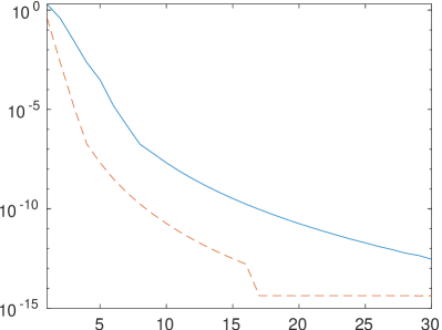
Figure 1: Graph of the two terms in inequality (11) for Example 1 (left) and Example 2 (right): $|S_{n_{1},n_{2}}|$ is represented by a continuous line, $\max(|\mathcal{E}^{(1)}_{n_{1},n_{2}}|,|\mathcal{E}^{(2)}_{n_{1},n_{2}}|)$ by a dashed one.

Example 2.

Let us consider integral (1) with

$$f(x_{1},x_{2})=x_{1}\left|\cos\left(\frac{1}{2}-x_{1}\right)\right|^{\frac{3}{2}}+x_{2}|\sin(1+x_{2})|^{\frac{3}{2}},$$

and

$$w(x_{1},x_{2})=\sqrt{\frac{1-x_{1}^{2}}{1-x_{2}}}.$$

In this case, the integrand function has a low smoothness with respect to both variables. Then, to obtain a good approximation we need to increase both $n_{1}$ and $n_{2}$. In Table 2, we can see the computational advantage of the averaged rule with respect to the Gauss scheme. To obtain an error of the order $10^{-13}$ we have two options: we may apply the averaged rule with $n_{1}=n_{2}=128$, and this requires $n_{1}n_{2}+(n_{1}+1)(n_{2}+1)=33.025$ function evaluations, or we may use the Gauss cubature formula with $n_{1}=n_{2}=256$. In this case, we have to perform $n_{1}n_{2}=65.536$ function evaluations.

Table 2: Cubature errors for Example 2.

$n_{1}$	$n_{2}$	$R^{(G)}_{n_{1},n_{2}}(f)$	$R^{(A)}_{n_{1},n_{2}}(f)$	$R^{(Avg)}_{n_{1},n_{2}}(f)$	$R^{[1]}_{n_{1},n_{2}}(f)$
2	2	-1.71e-01	1.71e-01	-6.53e-05	-1.71e-01
4	4	-7.14e-04	7.19e-04	2.45e-06	-7.16e-04
8	8	-1.53e-05	1.55e-05	9.05e-08	-1.54e-05
16	16	-4.66e-07	4.72e-07	2.98e-09	-4.69e-07
32	32	-1.49e-08	1.51e-08	9.62e-11	-1.50e-08
64	64	-4.73e-10	4.79e-10	3.07e-12	-4.76e-10
128	128	-1.49e-11	1.51e-11	1.13e-13	-1.50e-11
256	256	-4.51e-13	4.84e-13	1.60e-14	-4.67e-13
512	512	-6.22e-15	2.40e-14	8.88e-15	-1.51e-14

The graph on the right in Figure 1 shows that for some values of $n_{1}=n_{2}$ the assumption (11) of Theorem 2 is violated. However, numerical experiments show that the change of sign in the error always happens. In particular, the graph shows that inequality (11) is not verified when $n_{1}=n_{2}=20$, but we have $R^{(G)}_{20,20}(f)=-1.54\cdot 10^{-07}$ and $R^{(A)}_{20,20}(f)=1.56\cdot 10^{-07}$.

The assumption (11) is undoubtedly restrictive, but it is only a sufficient condition for the bracketing of the solution. In [7, Corollary 1] a less restrictive assumption has been given, in the univariate case, for the Chebychev weight of the first kind. The following corollary extends that result to bivariate integrals.

Corollary 3.

Let $\alpha_{i}=\beta_{i}=-\frac{1}{2}$ in (2). Then, if

$$\max(|\tilde{\mathcal{E}}^{(1)}_{n_{1},n_{2}}|,|\tilde{\mathcal{E}}^{(2)}_{n_{1},n_{2}}|)<|\alpha_{2n_{1},0}+\alpha_{0,2n_{2}}|,$$

holds true for $n_{1}$ and $n_{2}$ large enough, where

$$\tilde{\mathcal{E}}^{(1)}_{n_{1},n_{2}} =\sqrt{2}\alpha_{2n_{1},2n_{2}}+\sum_{k_{1}=2}^{\infty}(-1)^{k_{1}}\left(\alpha_{2n_{1}k_{1},0}-\sqrt{2}\,\alpha_{2n_{1}k_{1},2n_{2}}\right)$$

$$\phantom{=}+\sqrt{2}\sum_{k_{1}=2}^{\infty}\sum_{k_{2}=2}^{\infty}(-1)^{k_{1}+k_{2}}\alpha_{2n_{1}k_{1},2n_{2}k_{2}}+\sum_{k_{2}=2}^{\infty}(-1)^{k_{2}}\left(\alpha_{0,2n_{2}k_{2}}-\sqrt{2}\,\alpha_{2n_{1},2n_{2}k_{2}}\right),$$

and

$$\tilde{\mathcal{E}}^{(2)}_{n_{1},n_{2}} =\sqrt{2}\alpha_{2n_{1},2n_{2}}+\sum_{k_{1}=2}^{\infty}\left(\alpha_{2n_{1}k_{1},0}+\sqrt{2}\,\alpha_{2n_{1}k_{1},2n_{2}}\right)$$

$$\phantom{=}+\sqrt{2}\sum_{k_{1}=2}^{\infty}\sum_{k_{2}=2}^{\infty}\alpha_{2n_{1}k_{1},2n_{2}k_{2}}+\sum_{k_{2}=2}^{\infty}\left(\alpha_{0,2n_{2}k_{2}}+\sqrt{2}\,\alpha_{2n_{1},2n_{2}k_{2}}\right),$$

then the statement of Theorem 2 holds true.

Proof.

The identity

$$G_{n}(p_{i}^{(\ell)})=\begin{cases}(-1)^{k}\sqrt{2\pi},&\text{if $i=2nk$},\\ 0,&\text{otherwise},\end{cases}$$

reported in proof of Corollary 1 in [7], allows us to obtain a simplified expression for the terms $S_{n_{1},n_{2}}$, $\mathcal{E}^{(1)}_{n_{1},n_{2}}$ and $\mathcal{E}^{(2)}_{n_{1},n_{2}}$ given in Theorem 2, that is,

$$S_{n_{1},n_{2}}=\sqrt{2}\pi(\alpha_{2n_{1},0}+\alpha_{0,2n_{2}}),\quad\mathcal{E}^{(1)}_{n_{1},n_{2}}=\sqrt{2}\pi\tilde{\mathcal{E}}^{(1)}_{n_{1},n_{2}},\quad\mathcal{E}^{(2)}_{n_{1},n_{2}}=\sqrt{2}\pi\tilde{\mathcal{E}}^{(2)}_{n_{1},n_{2}}.$$

By applying Theorem 2, we conclude the proof. ∎

We remark here that, for the Chebychev case, the number of coefficients $\alpha_{i,j}$ present in the different series terms is much smaller than the ones involved in the completed expression of $|\mathcal{E}^{(1)}_{n_{1},n_{2}}|$ and $|\mathcal{E}^{(2)}_{n_{1},n_{2}}|$ introduced in the proof of Theorem 2, simplifying the relation (11).

In the next corollary, we further streamline the results in Corollary 3.

Corollary 4.

Let us consider $\alpha_{i}=\beta_{i}=-\frac{1}{2}$ in (2). Then, if

$$|\theta_{n_{1},n_{2}}|<|\alpha_{2n_{1},0}+\alpha_{0,2n_{2}}|,$$

holds true for $n_{1}$ and $n_{2}$ large enough, where

$$|\theta_{n_{1},n_{2}}| =\sqrt{2}|\alpha_{2n_{1},2n_{2}}|+\sum_{k_{1}=2}^{\infty}|\alpha_{2n_{1}k_{1},0}|+\sqrt{2}\,|\alpha_{2n_{1}k_{1},2n_{2}}|$$

$$+\sqrt{2}\sum_{k_{1}=2}^{\infty}\sum_{k_{2}=2}^{\infty}|\alpha_{2n_{1}k_{1},2n_{2}k_{2}}|+\sum_{k_{2}=2}^{\infty}|\alpha_{0,2n_{2}k_{2}}|+\sqrt{2}\,|\alpha_{2n_{1},2n_{2}k_{2}}|,$$

then the statement of Theorem 2 holds true.

Proof.

By using the triangle inequality and taking into account the hypothesis, we have

$$\max(|\tilde{\mathcal{E}}^{(1)}_{n_{1},n_{2}}|,|\tilde{\mathcal{E}}^{(2)}_{n_{1},n_{2}}|)\leq|\theta_{n_{1},n_{2}}|\leq|\alpha_{2n_{1},0}+\alpha_{0,2n_{2}}|,$$

which yields the assertion, by virtue of Theorem 2. ∎

3 Nyström methods and the averaged Nyström interpolant

The aim of this section is to approximate the solution of (3) by an interpolant function whose construction is based on Gauss and anti-Gauss cubature rules (6) and (7).

If the right hand side of (3) have algebraic singularities at $\pm 1$, the solution inherits the same singularities. The same happens if the kernel is singular at $\pm 1$ with respect to the external variables $(y_{1},y_{2})$. Therefore, we solve the equation in a suitable weighted space. Let us introduce the weight function

$$u({\mathbf{x}})=u_{1}(x_{1})u_{2}(x_{2}),$$ (12)

with

$$u_{i}(x_{i})=(1-x_{i})^{\gamma_{i}}(1+x_{i})^{\delta_{i}},\quad\gamma_{i},\delta_{i}\geq 0,\quad i=1,2.$$

We search for the solution of (3) in the space $C_{u}$ of all functions $f$ continuous in the interior of the square $\mathcal{S}$ and such that

$$\begin{cases}\displaystyle\lim_{x_{1}\to\pm 1}(fu)(x_{1},x_{2})=0,\qquad\forall x_{2}\in[-1,1],\\ \displaystyle\lim_{x_{2}\to\pm 1}(fu)(x_{1},x_{2})=0,\qquad\forall x_{1}\in[-1,1],\end{cases}$$

endowed with the norm

$$\|f\|_{C_{u}}=\|fu\|_{\infty}=\sup_{{\mathbf{x}}\in\mathcal{S}}|(fu)({\mathbf{x}})|.$$

If $\gamma_{i}=\delta_{i}=0$ for $i=1,2$, then $C_{u}$ coincides with the set of all continuous functions on the square, i.e., $C_{u}\equiv C(\mathcal{S})$. If the function $f$ has one or more singularities on the boundary of $\mathcal{S}$, then the corresponding parameter $\gamma_{i}$ or $\delta_{i}$ is set to a positive value in order to compensate the singularity.

This approach amounts to solving the weighted equation

$$(fu)({\mathbf{y}})-\int_{\mathcal{S}}k({\mathbf{x}},{\mathbf{y}})\frac{u({\mathbf{y}})}{u({\mathbf{x}})}(fu)({\mathbf{x}})w({\mathbf{x}})d{\mathbf{x}}=(gu)({\mathbf{y}}),$$ (13)

in the space $C(\mathcal{S})$ of continuous functions on the square.

To deal with smoother functions having some discontinuous derivatives on the boundary of $\mathcal{S}$, we introduce the Sobolev-type space

$$W^{r}_{u}=\{f\in C_{u}:\|f_{x_{i}}^{(r)}\varphi^{r}u\|_{\infty}<\infty,\ i=1,2\},$$

where $\varphi(z)=\sqrt{1-z^{2}}$. The superscript $(r)$ denotes the $r$th derivative of the univariate function $f_{x_{i}}$, obtained by fixing either $x_{1}$ or $x_{2}$ in the function $f$. We equip $W^{r}_{u}$ with the norm

$$\|f\|_{W^{r}_{u}}=\|fu\|_{\infty}+\max_{i=1,2}\|f_{x_{i}}^{(r)}\varphi^{r}u\|_{\infty}.$$

The error of best polynomial approximation in $C_{u}$ can be defined as

$$E_{m,n}(f)_{u}=\inf_{p\in\mathbb{P}_{m,n}}\|[f-p]u\|_{\infty}.$$

From now on, the symbol $\mathcal{C}$ will denote a positive constant and we will use the notation $\mathcal{C}\neq\mathcal{C}(a,b,\ldots)$ to say that $\mathcal{C}$ is independent of the parameters $a,b,\ldots$, and $\mathcal{C}=\mathcal{C}(a,b,\ldots)$ to say that it depends on them. Moreover, if $A,B>0$ are quantities depending on some parameters, we will write $A\sim B$, if there exists a positive constant $\mathcal{C}\neq\mathcal{C}(A,B)$ such that $\frac{B}{\mathcal{C}}\leq A\leq CB.$

Next proposition gives an estimate for the above error in Sobolev-type spaces.

Proposition 5.

For each $f\in W^{r}_{u}$, it holds

$$E_{m,n}(f)_{u}\leq\mathcal{C}\left[\frac{1}{m^{r}}+\frac{1}{n^{r}}\right]\cdot\max_{i=1,2}\|f_{x_{i}}^{(r)}\varphi^{r}u\|_{\infty},$$

where $\mathcal{C}\neq\mathcal{C}(m,n,f)$.

Proof.

Following [37, Theorem 2.1], one has

$$E_{m,n}(f)_{u}\leq\mathcal{C}\left[\sup_{x_{2}\in[-1,1]}u_{2}(x_{2})E_{m}(f_{x_{2}})_{u_{1}}+\sup_{x_{1}\in[-1,1]}u_{1}(x_{1})E_{n}(f_{x_{1}})_{u_{2}}\right],$$

where $E_{\ell}(g)_{u_{i}}$ is the $u_{i}$-weighted best approximation error of the univariate function $g$ by a polynomial of degree at most $\ell$; see [28, estimate (2.5.16)]. Then, by the inequality

$$E_{\ell}(g)_{u_{i}}\leq\frac{\mathcal{C}}{\ell^{r}}\|g^{(r)}\varphi^{r}u_{i}\|_{\infty},$$

from [28, estimate (2.5.22)], we obtain the assertion. ∎

To ease the exposition, we introduce a multi-index notation, where an index may take integer vectorial values. Such indexes will be denoted by bold letters. Let ${\mathbf{n}}=(n_{1},n_{2})$ and consider the set of bi-indices

$$\mathfrak{I}_{\mathbf{n}}=\left\{{\mathbf{i}}=(i_{1},i_{2}):1\leq i_{1}\leq n_{1},\,1\leq i_{2}\leq n_{2}\right\}.$$

For ${\mathbf{i}}\in\mathfrak{I}_{\mathbf{n}}$, consistently with the notation ${\mathbf{x}}=(x_{1},x_{2})$, we define ${\mathbf{x}}_{\mathbf{i}}=(x_{i_{1}}^{(1)},x_{i_{2}}^{(2)})$, where $x_{i_{1}}^{(1)}$ and $x_{i_{2}}^{(2)}$ are the Gaussian nodes introduced in the cubature rule (6), which we will denote by $\mathcal{G}_{\mathbf{n}}$.

Let us now write the classical Nyström method for the integral equation (3), based on approximating the operator $K$ by the Gauss cubature formula $\mathcal{G}_{\mathbf{n}}$. This leads to the functional equation

$$(I-K_{\mathbf{n}})f_{\mathbf{n}}=g,$$ (14)

where $f_{\mathbf{n}}$ is an unknown function approximating $f$ and

$$(K_{\mathbf{n}}f)({\mathbf{y}})=\sum_{j_{1}=1}^{n_{1}}\sum_{j_{2}=1}^{n_{2}}\lambda_{j_{1}}^{(1)}\lambda_{j_{2}}^{(2)}\,k({\mathbf{x}}_{\mathbf{j}},{\mathbf{y}})f({\mathbf{x}}_{\mathbf{j}}),$$

where $\mathbf{j}=(j_{1},j_{2})\in\mathfrak{I}_{\mathbf{n}}$.

By multiplying both sides of (14) by the weight function $u$ and collocating at the points ${\mathbf{x}}_{\mathbf{i}}$, ${\mathbf{i}}\in\mathfrak{I}_{\mathbf{n}}$, we obtain the linear system

$$\sum_{j_{1}=1}^{n_{1}}\sum_{j_{2}=1}^{n_{2}}\left[\delta_{i_{1},j_{1}}\delta_{i_{2},j_{2}}-\lambda_{j_{1}}^{(1)}\lambda_{j_{2}}^{(2)}\,\dfrac{u({\mathbf{x}}_{\mathbf{i}})}{u({\mathbf{x}}_{\mathbf{j}})}\,k({\mathbf{x}}_{\mathbf{j}},{\mathbf{x}}_{\mathbf{i}})\right]\,a_{j_{1},j_{2}}=(gu)({\mathbf{x}}_{\mathbf{i}}),$$ (15)

where $\delta_{i,k}$ is the Kronecker symbol, and $a_{j_{1},j_{2}}=(fu)({\mathbf{x}}_{\mathbf{j}})$ are the unknowns. By defining $\delta_{{\mathbf{i}},\mathbf{j}}=\delta_{i_{1},j_{1}}\delta_{i_{2},j_{2}}$, $\lambda_{\mathbf{j}}=\lambda_{j_{1}}^{(1)}\lambda_{j_{2}}^{(2)}$, and collapsing the two summations into a single one, (15) can be rewritten as

$$\sum_{\mathbf{j}\in\mathfrak{I}_{\mathbf{n}}}\left[\delta_{{\mathbf{i}},\mathbf{j}}-\lambda_{\mathbf{j}}\,\dfrac{u({\mathbf{x}}_{\mathbf{i}})}{u({\mathbf{x}}_{\mathbf{j}})}\,k({\mathbf{x}}_{\mathbf{j}},{\mathbf{x}}_{\mathbf{i}})\right]\,a_{\mathbf{j}}=(gu)({\mathbf{x}}_{\mathbf{i}}),\qquad{\mathbf{i}}\in\mathfrak{I}_{\mathbf{n}}.$$ (16)

This corresponds to the Nyström method for the weighted equation (13).

We remark that the quantities $k({\mathbf{x}}_{\mathbf{j}},{\mathbf{x}}_{\mathbf{i}})$ are entries $k_{i_{1},i_{2},j_{1},j_{2}}$ of a fourth order tensor $\mathcal{K}\in\mathbb{R}^{I_{1}\times I_{2}\times I_{1}\times I_{2}}$, where $I_{k}=\{1,2,\ldots,n_{k}\}$, $k=1,2$; see [24]. Moreover, the tensor-matrix product in (16) and the tensor-tensor product that will be used in next section corresponds to the so-called Einstein product [4, 12]. We prefer to adopt the multi-index formalism, used, e.g., in [46, 47, 48], because it is closer to the usual matrix notation.

The solution of system (16) provides the unique solution of equation (14) and vice-versa. In fact, if $a^{*}_{\mathbf{j}}$ is a solution of (16), then we can determine the weighted solution of (14) by the so-called Nyström interpolant

$$(f_{\mathbf{n}}u)({\mathbf{x}})=(gu)({\mathbf{x}})+u({\mathbf{x}})\sum_{\mathbf{j}\in\mathfrak{I}_{\mathbf{n}}}\frac{\lambda_{\mathbf{j}}}{u({\mathbf{x}}_{\mathbf{j}})}\,k({\mathbf{x}}_{\mathbf{j}},{\mathbf{x}})\,a^{*}_{\mathbf{j}}.$$ (17)

Vice-versa, if we evaluate (17) at the cubature points we obtain the solution of (16).

Now, we apply the Nyström method to the anti-Gaussian cubature formula $\mathcal{A}_{{\mathbf{n}}+\mathbf{1}}$, with $\mathbf{1}=(1,1)$, as an approximation for the operator $K$, obtaining the equation

$$(I-\widetilde{K}_{{\mathbf{n}}+\mathbf{1}})\tilde{f}_{{\mathbf{n}}+\mathbf{1}}=g,$$ (18)

where $\tilde{f}_{{\mathbf{n}}+\mathbf{1}}$ is the unknown and

$$(\widetilde{K}_{{\mathbf{n}}+\mathbf{1}}f)({\mathbf{y}})=\sum_{\mathbf{j}\in\mathfrak{I}_{{\mathbf{n}}+\mathbf{1}}}\mu_{\mathbf{j}}\,k(\boldsymbol{\eta}_{\mathbf{j}},{\mathbf{y}})f(\boldsymbol{\eta}_{\mathbf{j}}),$$

with $\mu_{\mathbf{j}}=\mu_{j_{1}}^{(1)}\mu_{j_{2}}^{(2)}$ and $\boldsymbol{\eta}_{\mathbf{j}}=(\eta_{j_{1}}^{(1)},\eta_{j_{2}}^{(2)})$.

A simple collocation of equation (18) at the knots $\boldsymbol{\eta}_{\mathbf{i}}$ and a multiplication of both sides by $u(\boldsymbol{\eta}_{\mathbf{i}})$ leads to the linear system

$$\sum_{\mathbf{j}\in\mathfrak{I}_{{\mathbf{n}}+\mathbf{1}}}\left[\delta_{{\mathbf{i}},\mathbf{j}}-\mu_{\mathbf{j}}\,\dfrac{u(\boldsymbol{\eta}_{\mathbf{i}})}{u(\boldsymbol{\eta}_{\mathbf{j}})}\,k(\boldsymbol{\eta}_{\mathbf{j}},\boldsymbol{\eta}_{\mathbf{i}})\right]\,\tilde{a}_{\mathbf{j}}=(gu)(\boldsymbol{\eta}_{\mathbf{i}}),\qquad{\mathbf{i}}\in\mathfrak{I}_{{\mathbf{n}}+\mathbf{1}}.$$ (19)

where $\tilde{a}_{\mathbf{j}}=(fu)(\boldsymbol{\eta}_{\mathbf{j}})$ are the unknowns.

If $\tilde{a}^{*}_{\mathbf{j}}$ is the solution of (19), then the Nyström interpolant

$$(\tilde{f}_{{\mathbf{n}}+\mathbf{1}}u)({\mathbf{x}})=(gu)({\mathbf{x}})+u({\mathbf{x}})\sum_{\mathbf{j}\in\mathfrak{I}_{{\mathbf{n}}+\mathbf{1}}}\frac{\mu_{\mathbf{j}}}{u(\boldsymbol{\eta}_{\mathbf{j}})}\,k(\boldsymbol{\eta}_{\mathbf{j}},{\mathbf{x}})\,\tilde{a}^{*}_{\mathbf{j}},$$ (20)

solves (18), and hence approximates the solution of (3). Vice-versa, if we evaluate the above function at the cubature points we obtain the solution of (19).

Theorem 6.

Let $\ker\{I+K\}=\{0\}$ in $C_{u}$ and let the parameters of the weight $u$ given in (12) be such that

$$0\leq\gamma_{i}<\alpha_{i}+1,\qquad 0\leq\beta_{i}<\delta_{i}+1,\qquad i=1,2.$$

We also assume that

$$g\in W_{u}^{r},\quad\sup_{{\mathbf{x}}\in\mathcal{S}}\|k_{{\mathbf{x}}}\|_{W^{r}_{u}}<\infty,\quad\sup_{{\mathbf{y}}\in\mathcal{S}}u({\mathbf{y}})\|k_{{\mathbf{y}}}\|_{W^{r}}<\infty.$$

Then, there exist a sufficiently large bi-index ${\mathbf{n}}_{0}$ such that, for ${\mathbf{n}}\geq{\mathbf{n}}_{0}$, equations (14) and (18) admit a unique solution $f^{*}_{\mathbf{n}}\in C_{u}$ and $\tilde{f}^{*}_{{\mathbf{n}}+\mathbf{1}}\in C_{u}$, respectively. Moreover, if $f^{*}$ is the unique solution of (3), then

$$\max\left\{\|(f^{*}-f^{*}_{\mathbf{n}})u\|_{\infty},\|(f^{*}-\tilde{f}^{*}_{{\mathbf{n}}+\mathbf{1}})u\|_{\infty}\right\}\leq\mathcal{C}\left[\frac{1}{n_{1}^{r}}+\frac{1}{n_{2}^{r}}\right]\cdot\max_{i=1,2}\|f_{x_{i}}^{*(r)}\varphi^{r}u\|_{\infty},$$ (21)

where $\mathcal{C}\neq\mathcal{C}({\mathbf{n}},f).$

Proof.

The stability of the Nyström method based on the Gauss rule as well as the error estimate (21) has been proved in [35] (see also [25, Theorem 4.1] for the case $u\equiv 1$). The proof of the assertion related to the Nyström method based on the anti-Gauss rule follows the same line of the corresponding theorem of [35]; see also [15, Theorem 3.1]. ∎

Corollary 7.

Let $f^{*}$ be the unique solution of (3). Consider the orthogonal expansion of the kernel $k$ multiplied by $f^{*}$ and its approximations $f_{\mathbf{n}}$ and $\tilde{f}_{{\mathbf{n}}+\mathbf{1}}$

$$k({\mathbf{x}},{\mathbf{y}})f^{*}({\mathbf{x}}) =\sum_{i=0}^{\infty}\sum_{j=0}^{\infty}\alpha_{i,j}({\mathbf{y}})p_{i,j}({\mathbf{x}}),\, \alpha_{i,j}({\mathbf{y}}) =\left(b_{0}^{(1)}b_{0}^{(2)}\right)^{-\frac{1}{2}}(K(f^{*}p_{i,j}))({\mathbf{y}}),$$

$$k({\mathbf{x}},{\mathbf{y}})f_{\mathbf{n}}({\mathbf{x}}) =\sum_{i=0}^{\infty}\sum_{j=0}^{\infty}\alpha_{i,j}^{\mathbf{n}}({\mathbf{y}})p_{i,j}({\mathbf{x}}),\, \alpha_{i,j}^{\mathbf{n}}({\mathbf{y}}) =\left(b_{0}^{(1)}b_{0}^{(2)}\right)^{-\frac{1}{2}}(K(f_{\mathbf{n}}p_{i,j}))({\mathbf{y}}),$$

$$k({\mathbf{x}},{\mathbf{y}})\tilde{f}_{{\mathbf{n}}+\mathbf{1}}({\mathbf{x}}) =\sum_{i=0}^{\infty}\sum_{j=0}^{\infty}\tilde{\alpha}_{i,j}^{{\mathbf{n}}+\mathbf{1}}({\mathbf{y}})p_{i,j}({\mathbf{x}}), \tilde{\alpha}_{i,j}^{{\mathbf{n}}+\mathbf{1}}({\mathbf{y}}) =\left(b_{0}^{(1)}b_{0}^{(2)}\right)^{-\frac{1}{2}}(K(\tilde{f}_{{\mathbf{n}}+\mathbf{1}}p_{i,j}))({\mathbf{y}}).$$

Then, under the assumption of Theorem 6,

$$\lim_{n_{1},n_{2}\to\infty}\|[\alpha_{i,j}^{\mathbf{n}}-\alpha_{i,j}]u\|_{\infty}=0\qquad\text{and}\qquad\lim_{n_{1},n_{2}\to\infty}\|[\tilde{\alpha}_{i,j}^{{\mathbf{n}}+\mathbf{1}}-\alpha_{i,j}]u\|_{\infty}=0.$$

Proof.

The proof follows the same line of Theorem 4 from [7]. ∎

Theorem 8.

Let us assume that inequality (11) is satisfied and the assumptions of Theorem 6 are verified. Then, for any ${\mathbf{y}}\in\mathcal{S}$, either

$$\tilde{f}_{{\mathbf{n}}+\mathbf{1}}({\mathbf{y}})\leq f^{*}({\mathbf{y}})\leq f_{\mathbf{n}}({\mathbf{y}})\quad\text{or}\quad f_{\mathbf{n}}({\mathbf{y}})\leq f^{*}({\mathbf{y}})\leq\tilde{f}_{{\mathbf{n}}+\mathbf{1}}({\mathbf{y}}).$$

Proof.

By (3), $f=Kf+g$. Proceeding similarly with equations (14) and (18), we deduce that to prove the assertion it is sufficient to state either of the following two relations

$$\begin{gathered}(\widetilde{K}_{{\mathbf{n}}+\mathbf{1}}\tilde{f}_{{\mathbf{n}}+\mathbf{1}})({\mathbf{y}})\leq(Kf^{*})({\mathbf{y}})\leq(K_{\mathbf{n}}f_{\mathbf{n}})({\mathbf{y}})\\ (K_{\mathbf{n}}f_{\mathbf{n}})({\mathbf{y}})\leq(Kf^{*})({\mathbf{y}})\leq(\widetilde{K}_{{\mathbf{n}}+\mathbf{1}}\tilde{f}_{{\mathbf{n}}+\mathbf{1}})({\mathbf{y}}).\end{gathered}$$

By virtue of the assumptions and Corollary 7, the above inequalities follow by applying Theorem 2 to the function $h_{\mathbf{y}}({\mathbf{x}})=k({\mathbf{x}},{\mathbf{y}})f({\mathbf{x}})$. ∎

Once we have proven under which conditions the unique solution $f^{*}$ of the integral equation is bracketed by the Nyström interpolants for any ${\mathbf{y}}\in\mathcal{S}$, we can introduce the averaged Nyström interpolant

$$\mathfrak{f_{\mathbf{n}}({\mathbf{y}})}=\dfrac{1}{2}\left(f_{\mathbf{n}}({\mathbf{y}})+\tilde{f}_{{\mathbf{n}}+\mathbf{1}}({\mathbf{y}})\right),\quad{\mathbf{y}}\in\mathcal{S},$$ (22)

which yields a better approximation of the solution.

4 Solving the linear systems

In this section we describe a tensor representation of systems (16) and (19), we study their condition number, and propose numerical methods for their resolution. In the following, the product between two tensors $\mathcal{M}$, $\mathcal{N}$, and between a tensor $\mathcal{M}$ and a matrix $\mathbf{a}$, must be considered in the multi-index sense, that is,

$$(\mathcal{M}\mathcal{N})_{{\mathbf{i}},\mathbf{j}}=\sum_{\mathsf{k}\in\mathfrak{I}_{\mathbf{n}}}\mathcal{M}_{{\mathbf{i}},\mathsf{k}}\mathcal{N}_{\mathsf{k},\mathbf{j}},\qquad(\mathcal{M}\mathbf{a})_{\mathbf{i}}=\sum_{\mathsf{k}\in\mathfrak{I}_{\mathbf{n}}}\mathcal{M}_{{\mathbf{i}},\mathsf{k}}\mathbf{a}_{\mathsf{k}},\qquad{\mathbf{i}},\mathbf{j}\in\mathfrak{I}_{\mathbf{n}}.$$

The inverse tensor is such that $\mathcal{M}\mathcal{M}^{-1}=\mathcal{I}$, where $(\mathcal{I})_{{\mathbf{i}},\mathbf{j}}=\delta_{{\mathbf{i}},\mathbf{j}}$. Moreover, the infinity norm $\|\mathcal{M}\|_{\infty}$ is defined in the usual operatorial sense, and the condition number is $\kappa_{\infty}(\mathcal{M})=\|\mathcal{M}\|_{\infty}\|\mathcal{M}^{-1}\|_{\infty}$.

Let us introduce the notation

$$\Lambda_{\mathbf{n}}=\mathop{\operator@font diag}\nolimits(\lambda_{\mathbf{j}})_{\mathbf{j}\in\mathfrak{I}_{\mathbf{n}}},\quad\text{with}\quad(\Lambda_{\mathbf{n}})_{{\mathbf{i}},\mathbf{j}}=\begin{cases}\lambda_{\mathbf{j}},&{\mathbf{i}}=\mathbf{j},\\ 0&{\mathbf{i}}\neq\mathbf{j}.\end{cases}$$

We give a compact representation of systems (16) and (19),

$$(\mathcal{I}_{\mathbf{n}}-\mathcal{U}_{\mathbf{n}}\mathcal{K}_{\mathbf{n}}\mathcal{U}_{\mathbf{n}}^{-1}\Lambda_{\mathbf{n}}){\mathbf{a}} ={\mathbf{h}},$$ (23)

$$(\mathcal{I}_{{\mathbf{n}}+\mathbf{1}}-\widetilde{\mathcal{U}}_{{\mathbf{n}}+\mathbf{1}}\widetilde{\mathcal{K}}_{{\mathbf{n}}+\mathbf{1}}\widetilde{\mathcal{U}}_{{\mathbf{n}}+\mathbf{1}}^{-1}\widetilde{\Lambda}_{{\mathbf{n}}+\mathbf{1}})\widetilde{{\mathbf{a}}} =\widetilde{{\mathbf{h}}},$$ (24)

where

$$\mathcal{K}_{{\mathbf{i}}\mathbf{j}}=k({\mathbf{x}}_{\mathbf{j}},{\mathbf{x}}_{\mathbf{i}})=k(x_{j_{1}}^{(1)},x_{j_{2}}^{(2)},x_{i_{1}}^{(1)},x_{i_{2}}^{(2)}),$$

$\mathcal{U}_{\mathbf{n}}=\mathop{\operator@font diag}\nolimits(u({\mathbf{x}}_{\mathbf{j}}))_{\mathbf{j}\in\mathfrak{I}_{\mathbf{n}}}$, and ${\mathbf{h}}=((gu)({\mathbf{x}}_{\mathbf{i}}))_{{\mathbf{i}}\in\mathfrak{I}_{\mathbf{n}}}$. Matrices $\widetilde{\mathcal{U}}_{{\mathbf{n}}+\mathbf{1}}$, $\widetilde{\mathcal{K}}_{{\mathbf{n}}+\mathbf{1}}$, $\widetilde{\Lambda}_{{\mathbf{n}}+\mathbf{1}}$, and the array $\widetilde{{\mathbf{h}}}$ are defined similarly.

In the next theorem we state the numerical stability of the Nyström method.

Theorem 9.

Under the assumptions of Theorem 6, it holds

$$\kappa_{\infty}(\mathcal{I}_{\mathbf{n}}-\mathcal{U}_{\mathbf{n}}\mathcal{K}_{\mathbf{n}}\mathcal{U}_{\mathbf{n}}^{-1}\Lambda_{\mathbf{n}})\leq\mathcal{C},\qquad\kappa_{\infty}(\mathcal{I}_{{\mathbf{n}}+\mathbf{1}}-\mathcal{U}_{{\mathbf{n}}+\mathbf{1}}\widetilde{\mathcal{K}}_{{\mathbf{n}}+\mathbf{1}}\widetilde{\mathcal{U}}_{{\mathbf{n}}+\mathbf{1}}^{-1}\widetilde{\Lambda}_{{\mathbf{n}}+\mathbf{1}})\leq\mathcal{C},$$

where $\mathcal{C}$ is independent of ${\mathbf{n}}$.

Proof.

The proof follows the same line of Theorem 3.1 from [35]. ∎

4.1 The general case

Let us first solve linear systems (23) and (24) in the general case, that is, when the coefficient tensor is not structured. For the sake of clarity and brevity, from now on we will only refer to system (23) and set

$$\mathcal{F}_{\mathbf{n}}=\mathcal{I}_{\mathbf{n}}-\mathcal{U}_{\mathbf{n}}\mathcal{K}_{\mathbf{n}}\mathcal{U}_{\mathbf{n}}^{-1}\Lambda_{\mathbf{n}}.$$

The same considerations will be valid for system (24) and the corresponding tensor $\widetilde{\mathcal{F}}_{{\mathbf{n}}+\mathbf{1}}$. We note that even if the kernel is a symmetric function like, for instance, $k({\mathbf{x}},{\mathbf{y}})={\mathbf{x}}^{2}+{\mathbf{y}}^{2}+{\mathbf{x}}{\mathbf{y}}$, the resulting coefficient tensor may not be not symmetric, that is, $(\mathcal{F}_{\mathbf{n}})_{{\mathbf{i}},\mathbf{j}}\neq(\mathcal{F}_{\mathbf{n}})_{\mathbf{j},{\mathbf{i}}}$, due to the presence of the weight function $u$ and the Christoffel numbers.

Before solving system (23), we rewrite it in matrix form, i.e., we transform the matrices containing the unknowns and the right-hand side into vectors, and represent the multi-index tensor as a standard matrix. To do this, we employ the lexicographical order to obtain the matrix $\mathbf{F}_{N}\in\mathbb{R}^{N\times N}$ given by

$$(\mathbf{F}_{N})_{\ell,k}=(\mathcal{F}_{\mathbf{n}})_{{\mathbf{i}},\mathbf{j}},\quad\ell=i_{1}+(i_{2}-1)n_{1},\quad k=j_{1}+(j_{2}-1)n_{1}.$$

This process is known as matricization or unfolding [24]. A similar procedure is applied to arrays $\mathbf{a}$ and $\mathbf{h}$ to obtain vectors $\bar{\mathbf{a}},\bar{\mathbf{h}}\in\mathbb{R}^{N}$, with $N=n_{1}n_{2}$, defined as

$$\bar{a}_{k}=a_{j_{1},j_{2}},\qquad\bar{h}_{k}=h_{j_{1},j_{2}},\qquad k=j_{1}+(j_{2}-1)n_{1},$$

for $j_{1}=1,\dots,n_{1}$, $j_{2}=1,\dots,n_{2}$, and $k=1,\dots,N$, so that the system becomes

$$\mathbf{F}_{N}\bar{\mathbf{a}}=\bar{\mathbf{h}}.$$ (25)

To solve system (25), we employ the generalized minimal residual (GMRES) method [41]. The GMRES iterative method for the solution of the linear system $\mathbf{F}_{N}\bar{\mathbf{a}}=\bar{\mathbf{h}}$ is based on the Arnoldi partial factorization

$$\mathbf{F}_{N}Q_{r}=Q_{r+1}H_{r+1,r},\qquad r=1,2,\ldots,N,$$

where $Q_{r}=[q_{1},q_{2},\ldots,q_{r}]$ has orthonormal columns, with $q_{1}=\bar{\mathbf{h}}/\|\bar{\mathbf{h}}\|$, and $H_{r+1,r}$ is an Hessenberg matrix; $\|\cdot\|$ denotes the vector 2-norm.

At the $r$th iteration, GMRES approximates the solution of the system as

$$\bar{\mathbf{a}}^{(r)}=\arg\min_{\bar{\mathbf{a}}\in K_{r}}\|\mathbf{F}_{N}\bar{\mathbf{a}}-\bar{\mathbf{h}}\|^{2}=\min_{y\in\mathbb{R}^{r}}\|H_{r+1,r}y-\|\bar{\mathbf{h}}\|\boldsymbol{{\mathrm{e}}}_{1}\|^{2},$$

where $K_{r}=\operatorname{span}\{\bar{\mathbf{h}},\mathbf{F}_{N}\bar{\mathbf{h}},\ldots,\mathbf{F}_{N}^{r-1}\bar{\mathbf{h}}\}=\operatorname{span}\{q_{1},\ldots,q_{r}\}$ is a Krylov space of dimension $r$.

Once the tensor $\mathcal{K}_{\mathbf{n}}$ has been computed, this requires $2N^{2}$ floating point operations to assemble the matrix $\mathbf{F}_{N}$ and a matrix-vector product at each iteration, leading to a computational cost of $O((2+r)N^{2})$.

The complexity can be slightly reduced by avoiding to assemble $\mathbf{F}_{N}$ and performing the product $\mathbf{F}_{N}\mathbf{q}_{k}$ at each iteration as

$$\mathbf{q}_{k}-\mathbf{u}\circ[K_{N}(\mathbf{d}\circ\mathbf{q}_{k})],$$

where $\mathbf{u}_{\mathbf{j}}=u(\mathbf{x}_{\mathbf{j}})$, $\mathbf{d}_{\mathbf{j}}=\lambda_{\mathbf{j}}/\mathbf{u}_{\mathbf{j}}$, $K_{N}$ is the matricization of $\mathcal{K}_{\mathbf{n}}$, and $\circ$ denotes the component-wise Hadamard product $(\mathbf{a}\circ\mathbf{b})_{\mathbf{j}}=\mathbf{a}_{\mathbf{j}}\mathbf{b}_{\mathbf{j}}$. In this case the computational cost is $O(rN^{2})$. We will denote this approach with a factored coefficient matrix by GMRES-FM.

4.2 The case of a separable kernel

Let us assume that the kernel in (3) is separable, that is,

$$k({\mathbf{x}},{\mathbf{y}})=k(x_{1},x_{2},y_{1},y_{2})=k_{1}(x_{1},y_{1})\,k_{2}(x_{2},y_{2}).$$

This means that $\mathcal{K}_{\mathbf{n}}=K^{(1)}_{n_{1}}\otimes K^{(2)}_{n_{2}}$, where $K^{(1)}_{n_{1}}$ and $K^{(2)}_{n_{2}}$ are two square matrices of dimension $n_{1}$ and $n_{2}$, respectively, with

$$(K^{(1)}_{n_{1}})_{i_{1},j_{1}}=k_{1}(x_{j_{1}}^{(1)},x_{i_{1}}^{(1)}),\qquad(K^{(2)}_{n_{2}})_{i_{2},j_{2}}=k_{2}(x_{j_{2}}^{(2)},x_{i_{2}}^{(2)}),$$

and $\otimes$ denotes the Kronecker tensor product, that is,

$$(\mathcal{K}_{\mathbf{n}})_{{\mathbf{i}},\mathbf{j}}=(K^{(1)}_{n_{1}})_{i_{1},j_{1}}(K^{(2)}_{n_{2}})_{i_{2},j_{2}}.$$

Keeping into account that $u({\mathbf{x}})=u_{1}(x_{1})u_{2}(x_{2})$ and $\lambda_{\mathbf{j}}=\lambda_{j_{1}}^{(1)}\lambda_{j_{2}}^{(2)}$, the system (16) becomes

$$\sum_{j_{1}=1}^{n_{1}}\sum_{j_{2}=1}^{n_{2}}\left[\delta_{i_{1},j_{1}}\delta_{i_{2},j_{2}}-\phi^{(1)}_{i_{1},j_{1}}\phi^{(2)}_{i_{2},j_{2}}\right]\,a_{j_{1},j_{2}}=h_{i_{1},i_{2}},$$

for $i_{1}=1,\ldots,n_{1}$ and $i_{2}=1,\ldots,n_{2}$, with

$$\phi^{(\ell)}_{i_{\ell},j_{\ell}}=\lambda^{(\ell)}_{j_{\ell}}\,\frac{u_{\ell}(x^{(\ell)}_{i_{\ell}})}{u_{\ell}(x^{(\ell)}_{j_{\ell}})}\,(K^{(\ell)}_{n_{\ell}})_{i_{\ell},j_{\ell}},\qquad\ell=1,2.$$

This amounts to solving the Stein matrix equation

$$\Phi^{(1)}A(\Phi^{(2)})^{T}-A+H=0,$$ (26)

where $A=(a_{j_{1},j_{2}})$, $H=(h_{i_{1},i_{2}})$, and $\Phi^{(\ell)}=(\phi^{(\ell)}_{i_{\ell},j_{\ell}})$, for $\ell=1,2$. There is a wide literature on numerical methods for solving this kind of matrix equations, some classical references are [3, 17, 19]. We will use the dlyap function of MATLAB.

The structure of the Stein equation (26) also allows for speeding up the GMRES method and reducing the storage space. Indeed, the product $\mathbf{F}_{N}\mathbf{q}_{k}$ can be expressed, at each iteration, in the form

$$Q_{k}-\Phi^{(1)}Q_{k}(\Phi^{(2)})^{T},$$

where the vector $\mathbf{q}_{k}$ is the unfolding of the matrix $Q_{k}$. In this way, the number of floating point operations of a matrix-vector product decreases from $O(N^{2})$ to $O(N)$, as well as the storage space. This implementation will be denoted in the following by GMRES-SK.

5 Numerical results

In this section we numerically solve several integral equations of the type (3) to investigate the performance of the method presented in Section 3 and Section 4, and support the theoretical analysis. For each example, we first identify the space $C_{u}$, in which the solution is sought, according to Theorem 6, solve systems (16) and (19), compute the Nyström interpolant (17) and (20), and calculate the averaged Nyström interpolant (22). The algorithms were implemented in Matlab version 9.10 (R2021a), and the numerical experiments were carried out on an Intel(R) Xeon(R) Gold 6136 server with 128 GB of RAM memory and 32 cores, running the Linux operating system.

To test the accuracy, we compute the relative errors

$$\xi^{(G)}_{{\mathbf{n}}}=\frac{\|f^{*}-f_{{\mathbf{n}}}\|_{C_{u}}}{\|f^{*}\|_{C_{u}}},\qquad\xi^{(A)}_{{\mathbf{n}}}=\frac{\|f^{*}-\tilde{f}_{{\mathbf{n}}+\mathbf{1}}\|_{C_{u}}}{\|f^{*}\|_{C_{u}}},\qquad\xi^{(Avg)}_{{\mathbf{n}}}=\frac{\|f^{*}-\mathfrak{f_{\mathbf{n}}}\|_{C_{u}}}{\|f^{*}\|_{C_{u}}},$$

where the infinity norm is approximated on a grid of $50\times 50$ points and $f^{*}$ is the exact solution of the equation. If the solution is unknown, then we consider as exact the approximated solution obtained by the Nyström interpolant (17) for sufficiently large $n_{1}$, $n_{2}$. The adopted value of ${\mathbf{n}}=(n_{1},n_{2})$ will be specified case by case.

In our tests, we consider both separable and non-separable kernels. When a low regularity of the kernel and/or the right-hand side yields the necessity of increasing the size of the linear system, we explore the efficiency of the proposed approaches for its solution methods, both in terms of accuracy and of computational time. In some examples, we report the $\infty$-norm condition numbers $\kappa_{\infty}^{(G)}$ and $\kappa_{\infty}^{(A)}$ of systems (24) and (23), respectively, to confirm the theoretical analysis of Theorem 9.

Example 3.

Let us first test our method on an integral equation whose exact solution is known. Consider the equation

$$f(y_{1},y_{2})-\int_{-1}^{1}\int_{-1}^{1}x_{2}y_{2}{\mathrm{e}}^{x_{1}+y_{1}}f(x_{1},x_{2})dx_{1}dx_{2}=g(y_{1},y_{2}),$$

with

$$g(y_{1},y_{2})=\cos{(y_{1}+y_{2})}-(\cos{2}+{\mathrm{e}}^{2}(\sin{2}-1))y_{2}{\mathrm{e}}^{y_{1}-1},$$

whose solution is $f(x_{1},x_{2})=\cos{(x_{1}+x_{2})}$. Since the kernel and right-hand side are smooth functions, we search for the solution in the space $C_{u}$ with $u\equiv 1$, i.e., we set $\gamma_{i}=\delta_{i}=0$ for $i=1,2$.

Table 3 reports the relative errors for increasing values of $n_{1}=n_{2}$. As expected, since the kernel and right-hand side are analytic functions, it shows a fast convergence. The averaged Nyström interpolant allows to improve accuracy up to four significant digits, with respect to the two Nyström interpolants based, respectively, on the Gauss and anti-Gauss rules. Since the size of the system is small, in this example we solve the linear systems by Gauss’s method with column pivoting. As highlighted by the last two columns of Table 3, the two systems are very well conditioned.

Table 3: Numerical results for Example 3.

${\mathbf{n}}$	$\xi^{(G)}_{{\mathbf{n}}}(f)$	$\xi^{(A)}_{{\mathbf{n}}}(f)$	$\xi^{(Avg)}_{{\mathbf{n}}}(f)$	$\kappa_{\infty}^{(G)}$	$\kappa_{\infty}^{(A)}$
(2,2)	3.79e-02	3.30e-02	2.43e-03	2.678	8.504
(4,4)	2.38e-06	2.38e-06	3.00e-10	19.016	30.849
(6,6)	2.50e-11	2.50e-11	1.33e-15	30.308	36.235
(8,8)	5.55e-16	9.99e-16	7.22e-16	34.967	34.941

A plot of the pointwise errors for the Gauss and the anti-Gauss interpolants is reported in Figure 2, for ${\mathbf{n}}=(4,4)$, in two different perspectives. It can be observed that the errors provided by the two cubature rules are of opposite sign, confirming the assertion of Theorem 8.

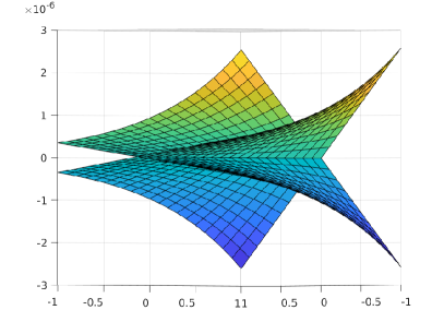
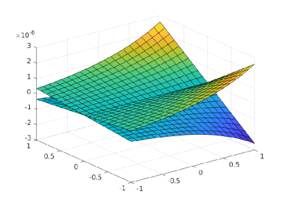
Figure 2: Error graphs for Example 3

Example 4.

In this example, we solve the integral equation

$$f(y_{1},y_{2})-\frac{3}{10}\int_{-1}^{1}\int_{-1}^{1}\sin{(x_{2}+x_{1})}(1+x_{1}+y_{2})f(x_{1},x_{2})w(x_{1},x_{2})dx_{1}dx_{2}=g(y_{1},y_{2}),$$

with

$$g(y_{1},y_{2})=\log{(2+y_{2})}\sin{(\sqrt{1-y_{1}})},$$

where $w(x_{1},x_{2})=\sqrt{1-x_{1}^{2}}$ ($\alpha_{1}=\frac{1}{2}$, $\beta_{1}=\frac{1}{2}$, $\alpha_{2}=0$, and $\beta_{2}=0$). According to Theorem 6, we fix $\gamma_{1}=1$, $\delta_{1}=\frac{5}{4}$, $\gamma_{2}=\frac{2}{3}$, and $\delta_{2}=\frac{2}{3}$ for the weight $u$ of the function space. Here, the exact solution $f^{*}$ is not available, so we approximate it by the Nyström interpolant based on the Gaussian formula with ${\mathbf{n}}=(700,32)$. The kernel is a smooth non-separable function whereas, for each fixed $y_{2}$, $g_{y_{2}}(y_{1})\in W_{3}$; therefore, by virtue of (21), the expected order of convergence is $O(n_{1}^{-3})$. Note that since the right-hand side has a different degree of smoothness with respect to the two variables, we can use a number of nodes $n_{2}$ much smaller than $n_{1}$, thus reducing the number of equations of the system. However, the low smoothness of the right-hand side causes $n_{1}$ to grow. So the size of the linear systems is moderately large, and we solve them by the GMRES-FM method, that is, the implementation with a factored coefficient matrix.

Table 4 reports the obtained relative errors. In this example the good performance of the averaged interpolant in term of accuracy is evident. To compute it, when ${\mathbf{n}}=(128,16)$, we have to solve two linear systems of order $128\cdot 16=2048$, with an error of order $10^{-11}$. The same error is produced by the Nyström method based on the Gauss rule, as reported in Table 4, but this requires to solve a system of order $256\cdot 16=4096$, and so a much larger complexity and storage space.

We see that GMRES-FM converges in few iterations (reported, in parentheses, in the second and third columns) and it is clear that the order of the system has no effect on the speed of convergence. In accordance with Theorem 9, this happens because the condition number of the coefficient matrices is small and does not depend on the size of the systems; see the last two columns of Table 4.

Table 4: Numerical results for Example 4.

${\mathbf{n}}$	$\xi^{(G)}_{{\mathbf{n}}}(f)$ (iter)	$\xi^{(A)}_{{\mathbf{n}}}(f)$ (iter)	$\xi^{(Avg)}_{{\mathbf{n}}}(f)$	$\kappa_{\infty}^{(G)}$	$\kappa_{\infty}^{(A)}$
(2,16)	8.12e-03 (3)	7.55e-03 (3)	2.86e-04	4.027	26.364
(4,16)	4.77e-04 (3)	4.22e-04 (3)	2.78e-05	20.280	39.241
(8,16)	4.26e-05 (3)	3.74e-05 (3)	2.61e-06	26.498	48.749
(16,16)	3.28e-06 (3)	2.88e-06 (3)	2.04e-07	32.148	51.621
(32,16)	2.30e-07 (3)	2.01e-07 (3)	1.44e-08	36.045	54.606
(64,16)	1.53e-08 (3)	1.34e-08 (3)	9.52e-10	38.933	56.108
(128,16)	9.82e-10 (3)	8.62e-10 (3)	6.03e-11	40.998	57.277
(256,16)	6.13e-11 (3)	5.57e-11 (3)	2.78e-12	42.433	58.044
(512,16)	2.80e-12 (3)	4.57e-12 (3)	8.80e-13	43.442	58.591

Example 5.

Let us now consider the following equation with a separable kernel

$$f(y_{1},y_{2})-\frac{3}{10}\int_{-1}^{1}\int_{-1}^{1}{\mathrm{e}}^{-(1+x_{1})(1+y_{1})-(1+y_{2})(1+x_{2})}f(x_{1},x_{2})w(x_{1},x_{2})dx_{1}dx_{2}=g(y_{1},y_{2}),$$

with a right-hand side characterized by a low degree of smoothness with respect to both variables

$$g(y_{1},y_{2})=\cos{(3+y_{2})}\,(1+y_{2})^{\frac{3}{2}}\,\sin\left((1-y_{1})^{\frac{3}{2}}\right),$$

where $w(x_{1},x_{2})=\sqrt{(1-x_{1}^{2})(1-x_{2}^{2})}$ with $\alpha_{1}=\beta_{1}=\frac{1}{2}$ and $\alpha_{2}=\beta_{2}=\frac{1}{2}$. For the weight $u$, we set $\gamma_{1}=\delta_{1}=\frac{5}{4}$ and $\gamma_{2}=\delta_{2}=\frac{5}{4}$.

In this test, we investigate the computational time required for solving the linear systems by Gauss’s method ($PA=LU$) and the four approaches described in the previous section: GMRES, GMRES-FM, where the coefficient matrix is multiplied in a factored form, GMRES-SK, specially suited for the case of a separable kernel, and the solution of Stein’s equation (26) by the dlyap function of MATLAB.

As highlighted in Table 5, the application of Gauss’s method, the standard implementation of GMRES, and GMRES-FM, are unfeasible when the system becomes moderately large. Moreover, the first three methods go out of memory when $n_{1},n_{2}>128$. On the contrary, GMRES-SK has a good performance and the computational time is comparable with that of MATLAB solver function dlyap. Both method can be applied for large problem dimensions.

Table 5: Computing times in seconds for Example 5.

${\mathbf{n}}$	$PA=LU$	GMRES	GMRES-FM	GMRES-SK	dlyap
(2,2)	0.0031	0.0044	0.0038	0.0048	0.0097
(4,4)	0.0061	0.0068	0.0067	0.0063	0.0064
(8,8)	0.0265	0.0234	0.0248	0.0230	0.0246
(16,16)	0.0784	0.0849	0.0864	0.0716	0.0705
(32,32)	0.3703	0.3070	0.2928	0.1905	0.1736
(64,64)	7.9212	7.2356	3.7162	2.8094	3.0727
(128,128)	59.0927	41.9451	18.9175	8.3955	8.4749
(256,256)	-	-	-	26.8196	26.1663
(512,512)	-	-	-	128.1439	121.2557

Table 6 reports the relative errors with respect to the approximation obtained setting ${\mathbf{n}}=(512,512)$, which we consider exact. The linear system is solved by the GMRES-SK method. The averaged Nyström interpolant provides 2 additional significant digits with respect to the base interpolants starting from ${\mathbf{n}}=(4,4)$, until it reaches machine precision for ${\mathbf{n}}=(128,128)$, while the approximation based on the standard Gauss cubature rule produces the same approximation for ${\mathbf{n}}=(256,256)$.

It is also important to remark that, if the assertion of Theorem 8 holds, the halved difference between the Gauss and anti-Gauss interpolants yields a bound for the approximation error of the averaged interpolant, that is,

$$\|f^{*}-\mathfrak{f_{\mathbf{n}}}\|_{\infty}\leq\frac{\|f_{{\mathbf{n}}}-\tilde{f}_{{\mathbf{n}}+\mathbf{1}}\|_{\infty}}{2}.$$

Such a bound is not directly available when a single formula is employed.

Table 6: Numerical results for Example 5.

${\mathbf{n}}$	$\xi^{(G)}_{{\mathbf{n}}}(f)$	$\xi^{(A)}_{{\mathbf{n}}}(f)$	$\xi^{(Avg)}_{{\mathbf{n}}}(f)$
(2,2)	3.41e-03	3.50e-03	1.41e-04
(4,4)	1.80e-05	1.78e-05	1.33e-07
(8,8)	2.48e-07	2.40e-07	3.97e-09
(16,16)	5.60e-09	5.42e-09	8.77e-11
(32,32)	1.05e-10	1.02e-10	1.64e-12
(64,64)	1.80e-12	1.74e-12	2.81e-14
(128,128)	2.94e-14	2.87e-14	5.29e-16
(256,256)	8.82e-16	9.71e-16	2.65e-16

Example 6.

In this example, we analyze the effect of a smooth right-hand side and a kernel which is not smooth with respect to the first variable. Hence, we apply our method to the equation

$$f(y_{1},y_{2})-\frac{1}{7}\int_{-1}^{1}\int_{-1}^{1}(x_{2}+y_{2})|\cos(1+x_{1})|^{\frac{9}{2}}f(x_{1},x_{2})w(x_{1},x_{2})dx_{1}dx_{2}=g(y_{1},y_{2}),$$

where

$$g(y_{1},y_{2})={\mathrm{e}}^{y_{1}}\sin{y_{2}},$$

$w(x_{1},x_{2})=\frac{\sqrt{1-x_{2}^{2}}}{\sqrt{1-x_{1}}}$ ($\alpha_{1}=-\frac{1}{2}$, $\beta_{1}=0$, $\alpha_{2}=\frac{1}{2}$, and $\beta_{2}=\frac{1}{2}$), and we fix $\gamma_{1}=0$, $\delta_{1}=\frac{1}{4}$, $\gamma_{2}=\frac{1}{2}$, and $\delta_{2}=\frac{5}{4}$, for the weight $u$ of the function space defined in (12). Also in this case the exact solution $f(x_{1},x_{2})$ is not available, so we approximate it by the Nyström interpolant based on the Gauss rule with ${\mathbf{n}}=(512,32)$.

Table 7 displays in the second and third columns the numerical errors provided by the Gauss and anti-Gauss Nyström methods. The results are better than the theoretical estimate, which is of order $O(n_{1}^{-4})$. The accuracy of the averaged interpolant improves of 1–2 significant digits, until machine precision is reached.

Table 7: Numerical results for Example 6

${\mathbf{n}}$	$\xi^{(G)}_{{\mathbf{n}}}(f)$	$\xi^{(A)}_{{\mathbf{n}}}(f)$	$\xi^{(Avg)}_{{\mathbf{n}}}(f)$
(2,16)	7.52e-04	6.85e-04	3.34e-05
(4,16)	1.33e-05	1.35e-05	8.22e-08
(8,16)	1.87e-07	1.79e-07	3.70e-09
(16,16)	4.71e-09	4.92e-09	1.05e-10
(32,16)	8.90e-11	8.99e-11	4.97e-13
(64,16)	5.44e-13	6.32e-13	4.39e-14
(128,16)	2.49e-14	2.65e-14	8.34e-16
(256,16)	9.12e-16	1.17e-15	1.56e-16

6 Conclusion and extensions

This paper introduces a new anti-Gauss cubature rule and proposes its application to the resolution of Fredholm integral equations of the second kind defined on the square. A Nyström-type method based on Gauss and anti-Gauss cubature rules is developed and analyzed in terms of stability and convergence, and an averaged Nyström interpolant is proposed to better approximate the solution of the problem. Numerical tests investigate the performance of the methods and confirm the computational advantage of the averaged Nyström interpolant, in comparison with the classical approach based on the Gauss rule. Extensions to other averaged cubature formulae are presently being developed by the authors.

References

- [1] A. Alipanah and S. Esmaeili, Numerical solution of the two-dimensional Fredholm integral equations using Gaussian radial basis function, J. Comput. Appl. Math., 235 (2011), pp. 5342–5347.
- [2] K. Atkinson, D. D.-K. Chien, and J. Seol, Numerical analysis of the radiosity equation using the collocation method, Electron. Trans. Numer. Anal., 11 (2000), pp. 94–120.
- [3] A. Barraud, A numerical algorithm to solve , IEEE Trans. Autom. Control, 22 (1977), pp. 883–885.
- [4] M. Brazell, N. Li, C. Navasca, and C. Tamon, Solving multilinear systems via tensor inversion, SIAM J. Matr. Anal. Appl., 34 (2013), pp. 542–570.
- [5] D. Calvetti, L. Reichel, and F. Sgallari, Applications of anti-Gauss quadrature rules in linear algebra, in Applications and Computation of Orthogonal Polynomials, W. Gautschi, G. H. Golub, and G. Opfer, eds., Birkhauser, Basel, 1999, pp. 41–56.
- [6] R. Cools, Constructing cubature formulae: The science behind the art, Acta Numer., 6 (1997), pp. 1–54.
- [7] P. Díaz de Alba, L. Fermo, and G. Rodriguez, Solution of second kind Fredholm integral equations by means of Gauss and anti-Gauss quadrature rules, Numer. Math., 146 (2020), pp. 699–728.
- [8] D. L. Djukić, L. Fermo, and R. M. Mutavdžić Djukić, Averaged cubature schemes on the real positive semiaxis, Numer. Algorithms, 92 (2023), pp. 545–569.
- [9] D. L. Djukić, R. M. Mutavdzić Djukić, L. Reichel, and M. M. Spalević, Internality of generalized averaged Gauss quadrature rules and truncated variants for modified Chebyshev measures of the first kind, J. Comput. Appl. Math., 398 (2021), p. 113696.
- [10] D. L. Djukić, L. Reichel, and M. M. Spalević, Truncated generalized averaged Gauss quadrature rules, J. Comput. Appl. Math., 308 (2016), pp. 408–418.
- [11] C. F. Dunkl and Y. Xu, Orthogonal Polynomials of Several Variables, Encyclopedia of Mathematics and its Applications, Cambridge University Press, 2 ed., 2014.
- [12] A. Einstein, The foundation of the general theory of relativity, Annalen Phys., 49 (1916), pp. 769–822.
- [13] C. Fenu, D. Martin, L. Reichel, and G. Rodriguez, Block Gauss and anti-Gauss quadrature with application to networks, SIAM J. Matrix Anal. Appl., 34 (2013), pp. 1655–1684.
- [14] L. Fermo, L. Reichel, G. Rodriguez, and M. M. Spalević, Averaged Nyström interpolants for the solution of Fredholm integral equations of the second kind, Appl. Math. Comput., (2023). To appear. Available at https://arxiv.org/abs/2307.11601.
- [15] L. Fermo and M. G. Russo, Numerical methods for Fredholm integral equations with singular right-hand sides, Adv. Comput. Math., 33 (2010), pp. 305–330.
- [16] W. Gautschi, Orthogonal polynomials. Computation and Approximation, Numerical Mathematics and Scientific Computation, Oxford University Press, Oxford, 2004.
- [17] G. Golub, S. Nash, and C. Van Loan, A Hessenberg-Schur method for the problem , IEEE Trans. on Autom. Control, 24 (1979), pp. 909–913.
- [18] G. Golub and J. H. Welsch, Calculation of Gauss quadrature rules, Math. Comp., 23 (1969), pp. 221–230.
- [19] S. J. Hammarling, Numerical solution of the stable, non-negative definite Lyapunov equation, IMA J. Numer. Anal., 2 (1982), pp. 303–323.
- [20] G. Han and R. Wang, Richardson extrapolation of iterated discrete Galerkin solution for two-dimensional Fredholm integral equations, J. Comput. Appl. Math., 139 (2002), pp. 49–63.
- [21] S. Hatamzadeh-Varmazyar and Z. Masouri, Numerical method for analysis of one- and two-dimensional electromagnetic scattering based on using linear Fredholm integral equation models, Math. Comput. Model., 54 (2011), pp. 2199–2210.
- [22] H. B. Jebreen, A novel and efficient numerical algorithm for solving 2d Fredholm integral equations, J. Math., 2020 (2020).
- [23] J. T. Kajiya, The rendering equation, in Proceedings of the 13th annual conference on Computer graphics and interactive techniques, 1986, pp. 143–150.
- [24] T. G. Kolda and B. W. Bader, Tensor decompositions and applications, SIAM Rev., 51 (2009), pp. 455–500.
- [25] A. L. Laguardia and M. G. Russo, Numerical methods for Fredholm integral equations based on Padua points, Dolomit. Res. Notes Approx., 15 (2022), pp. 65–77.
- [26] D. P. Laurie, Anti-Gaussian quadrature formulas, Math. Comp., 65 (1996), pp. 739–747.
- [27] Y. Ma, J. Huang, and H. Li, A novel numerical method of two-dimensional Fredholm integral equations of the second kind, Math. Probl. Eng., 2015 (2015).
- [28] G. Mastroianni and G. V. Milovanović, Interpolation Processes: Basic Theory and Applications, Springer Monographs in Mathematics, Springer Verlag, Berlin, 2008.
- [29] F. Mirzaee and E. Hadadiyan, Numerical solution of linear Fredholm integral equations via two-dimensional modification of hat functions, Appl. Math. Comput., 250 (2015), pp. 805–816.
- [30] C. R. Morrow and T. N. L. Patterson, Construction of algebraic cubature rules using polynomial ideal theory, SIAM J. Numer. Anal., 15 (1978), pp. 953–976.
- [31] I. P. Mysovskikh, Numerical characteristics of orthogonal polynomials in two variables, Vestnik Leningrad Univ. Math., 3 (1976), pp. 323–332.
- [32] S. E. Notaris, Gauss-Kronrod quadrature formulae - a survey of fifty years of research, Electron. Trans. Numer. Anal., 45 (2016), pp. 371–404.
- [33] , Anti-Gaussian quadrature formulae based on the zeros of Stieltjes polynomials, BIT, 58 (2018), pp. 179–198.
- [34] , Anti-Gaussian quadrature formulae of Chebyshev type, Math. Comp., 91 (2022), p. 2803 – 2816.
- [35] D. Occorsio and M. G. Russo, Numerical methods for Fredholm integral equations on the square, Appl. Math. Comput., 218 (2011), pp. 2318–2333.
- [36] , Bivariate Generalized Bernstein operators and their application to Fredholm integral equations, Publ. Inst. Math.-Beograd, 100 (2016), pp. 141–162.
- [37] , Nyström methods for bivariate Fredholm integral equations on unbounded domains, Appl. Math. and Comput., 318 (2018), pp. 19–34.
- [38] M. S. Pranić and L. Reichel, Generalized anti-Gauss quadrature rules, J. Comput. Appl. Math., 284 (2015), pp. 235–243.
- [39] L. Reichel and M. M. Spalević, A new representation of generalized averaged Gauss quadrature rules, Appl. Numer. Math., 165 (2021), pp. 614–619.
- [40] L. Reichel and M. M. Spalević, Averaged Gauss quadrature formulas: Properties and applications, J. Comput. Appl. Math., 410 (2022).
- [41] Y. Saad and M. H. Schultz, GMRES: A generalized minimal residual algorithm for solving nonsymmetric linear systems, SIAM J. Sci. Stat. Comput., 7 (1986), pp. 856–869.
- [42] H. J. Schmid, On cubature formulae with a minimal number of knots, Numer. Math., 31 (1978), pp. 281–297.
- [43] H. J. Schmid and Y. Xu, On Bivariate Gaussian Cubature Formulae, Proc. Amer. Math. Soc., 122 (1994), pp. 833–841.
- [44] M. M. Spalević, On generalized averaged Gaussian formulas, Math. Comp., 76 (2007), pp. 1483–1492.
- [45] A. H. Stroud, Approximate calculation of multiple integrals, Prentice-Hall, Englewood Cliffs, 1971.
- [46] C. V. M. van der Mee, G. Rodriguez, and S. Seatzu, Semi-infinite multi-index perturbed block Toeplitz systems, Linear Algebra Appl., 366 (2003), pp. 459–482.
- [47] , Fast computation of two-level circulant preconditioners, Numer. Algorithms, 41 (2006), pp. 275–295.
- [48] , Fast superoptimal preconditioning of multiindex Toeplitz matrices, Linear Algebra Appl., 418 (2006), pp. 576–590.
- [49] Y. Wang and Y. Xu, A fast wavelet collocation method for integral equations on polygons, J. Integral Equ. Appl., 17 (2005), pp. 277–330.
- [50] Y. Xu, Minimal cubature rules and polynomial interpolation in two variables, J. Approx. Theory, 164 (2012), pp. 6–30.
- [51] , Generalized characteristic polynomials and Gaussian cubature rules, SIAM J. Matrix Anal. Appl., 36 (2015), p. 1129 – 1142.