FLASC: A Flare-Sensitive Clustering Algorithm

Abstract.

We present FLASC, an algorithm for flare-sensitive clustering. Our algorithm builds upon HDBSCAN*—which provides high-quality density-based clustering performance—through a post-processing step that differentiates branches within the detected clusters’ manifold, adding a type of pattern that can be discovered. Two variants of the algorithm are presented, which trade computational cost for noise robustness. We show that both variants scale similarly to HDBSCAN* in terms of computational cost and provide stable outputs using synthetic data sets, resulting in an efficient flare-sensitive clustering algorithm. In addition, we demonstrate the algorithm’s benefit in data exploration over HDBSCAN* clustering on two real-world data sets.

Figure 1. Weighted cluster segmentation for HDBSCAN* (left) and FLASC (right). FLASC distinguishes flares in clusters with distinct labels. Point cloud adapted from HDBSCAN*’s online tutorial pages (McInnes et al., 2017, 2022).

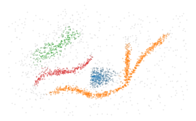
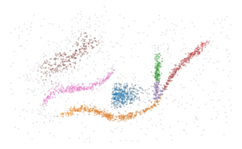
Two scatterplots with points coloured by their cluster membership strength. HDBSCAN* detects the Y-shaped cluster as a single subgroup. FLASC detects four subgroups within that cluster: one for each branch and one for the centre where the branches merge.

1. Introduction

Exploratory Data Analysis (EDA)—i.e., searching for interesting patterns in data—is ubiquitous in data science and knowledge discovery workflows. Detecting which subpopulations exist in a data set is a common step in EDA. Not only clusters but also their shapes can reveal relevant subgroups. Specifically, flares—i.e. the branches in a cluster’s manifold—can represent meaningful subpopulations (f.i., see (Lum et al., 2013; Skaf and Laubenbacher, 2022; Kamruzzaman et al., 2018; Reaven and Miller, 1979)). Informally, flares are attachments to a cluster’s core, such as the Y-shaped cluster’s branches in Figure 1.

Several data exploration techniques exist that can detect such branch-based subgroups. Structure learning algorithms—such as Bonnaire et al.’s mixture model approach (Bonnaire et al., 2022) and Mao et al.’ Reversed Graph Embedding (Mao et al., 2017)—model a data set’s principal curve as a graph representing the paths through the middle of the point cloud. These algorithms can, for example, extract road networks from GPS car position samples (Bonnaire et al., 2022) or describe developmental trajectories in single-cell gene expression data (Qiu et al., 2017; Mao et al., 2017). The resulting graphs can also partition the data by the segments between their intersections to detect flare-sensitive subgroups (Chervov et al., 2020). Mapper (Singh et al., 2007) summarises a data set’s structure over manually-specified lens dimensions allowing researchers to inject their domain knowledge into the analysis. The algorithm has been used successfully for finding patterns that previously went unnoticed (Lum et al., 2013; Skaf and Laubenbacher, 2022). When a centrality metric is used as lens dimension, Mapper’s output graph describes the data’s branching structure from which flare-sensitive subgroups can be extracted (f.i. see (Kamruzzaman et al., 2018; Madhobi et al., 2019)).

Clustering algorithms, on the other hand, generally cannot detect this type of subgroup because there is no gap that separates flares from their cluster (Carlsson, 2014). For example, HDBSCAN* (Campello et al., 2013, 2015)—which provides state-of-the-art density-based clustering performance—detects the Y-shaped orange cluster in Figure 1 as a single entity. In the present paper, we extend HDBSCAN* with a flare-detection post-processing step to enable it to detect branch-based subgroups (for example, see Figure 1). This approach provides several benefits: (1) operating on the clusters found by HDBSCAN* reduces the effects of noisy observations, and (2) not building an explicit model of the data’s structure avoids computational costs. We call the resulting algorithm Flare-Sensitive Clustering (FLASC). We empirically analyse its computational cost and stability on synthetic data sets to show that the cost of detecting flares is relatively low. In addition, we demonstrate FLASC on two real-world data sets, illustrating its benefits for data exploration.

In the remainder of this section, we discuss related work and our contributions. Section 2 briefly recaps the HDBSCAN* clustering algorithm. Section 3 describes how FLASC builds on HDBSCAN* to detect branches within clusters and discusses the algorithm’s complexity and stability. Section 4 presents our empirical analyses that show how the algorithm behaves. Finally, Sections 5 and 6 discuss our results and present our conclusions.

1.1. Clustering for Exploratory Data Analysis

Currently, HDBSCAN* (Campello et al., 2013, 2015) provides state-of-the-art clustering performance. The algorithm is well suited for exploring unfamiliar data because—unlike older popular clustering algorithms—HDBSCAN* does not require the number of clusters or the distance between clusters to be specified in advance. Additionally, the algorithm is robust to noise and makes no assumptions about the data’s underlying distribution.

HDBSCAN* is a density-based clustering algorithm. Informally, density-based clustering specifies clusters as regions of high density separated by regions of lower density. Visually, this notion is very intuitive. For example, even without the colours, one could easily differentiate the clusters from the noise in Figure 1. In addition, density-based clusters are not limited to convex shapes, and the formulation provides a natural way to separate noise points from clusters.

The principles of density-based clustering were pioneered by Wishart in (1969) (Wishart, 1969). In that article, Wishart presents One Level Mode Analysis, the—to our knowledge—first clustering algorithm based on non-parametric density estimation (as mentioned in (Campello et al., 2015)). Hartigan later formalised the concepts of density contour clusters and density contour trees (Hartigan, 1975), which underpin all density-based clustering algorithms in some form (Campello et al., 2015). The latter concept can also be viewed from a topological perspective, as the split tree constructed in a filtration over the density. See, for example, Figure 2, which shows a 1D continuous density profile with the resulting density contour clusters and density contour tree.

Since HDBSCAN*’s introduction, several studies have implemented and adapted the algorithm: McInnes and Healy (McInnes and Healy, 2017) improved the algorithm’s computational performance by using space trees for finding the data points’ nearest neighbours and provide a popular and efficient Python implementation (McInnes et al., 2017). Stewart and Al-Khassaweneh (Stewart and Al-Khassaweneh, 2022) created a Java implementation with a novel prediction technique for unseen data points. Jackson et al. (Jackson et al., 2018) presented an approximate HDBSCAN* algorithm that uses NN-descent (Dong et al., 2011) for finding the nearest neighbours providing fast distributed performance. Malzer and Baum (Malzer and Baum, 2020) introduced a cluster selection distance threshold that effectively creates a hybrid between DBSCAN’s (Ester et al., 1996) and HDBSCAN*’s cluster selection, improving the algorithm’s performance on data sets with small clusters and a large density variability. Neto et al. (Neto et al., 2021) showed how Relative Neighbourhood Graphs (RNGs) (Toussaint, 1980) can be used to efficiently compute HDBSCAN* cluster hierarchies for multiple min cluster size values. Their follow-up work presented MustaCHE, a visualisation tool for the resulting meta-cluster hierarchy (Neto et al., 2018). To our knowledge, no previous study has adapted HDBSCAN* for detecting flares.

1.2. Flare Detection

As mentioned before, clustering algorithms generally cannot detect flares within clusters. Using Figure 1 as an example, the Y-shaped cluster is found as a single entity by HDBSCAN*. This is expected because no lower-density region separates the flares. In other words, there is a path between data points in different branches that exclusively goes through data points ‘that lie close together’. From a topological perspective, as explained by Carlsson (Carlsson, 2014), clustering algorithms capture the 0-dimensional homology of the data space. That is, clustering describes the connected components in a simplicial complex of the data. Flares are connected in the simplicial complex. Therefore, they have a vanishing homology and cannot be detected as clusters.

It should be noted, though, that implicit in this argument is the assumption that the density across flares is constant (or decreasing). Subpopulations in real-world data sets tend to have some location in feature space where observations are more likely. These locations are detectable as local density maxima forming distinct clusters in a density contour tree, allowing the data points surrounding them to be classified as a particular subgroup. The corresponding cluster hierarchy, however, does not describe the data’s branching structure; it only detects the presence of these local maxima.

Having observed that data sets tend to have a central core connecting everything, Carlsson (Carlsson, 2014) proposes functional persistence to detect branches. The underlying idea is to remove the ‘core’ of the data set, separating branches from each other and making them detectable as clusters (see Figure 3). Carlsson (Carlsson, 2014) provides a centrality measure based on each data point’s distances sum to specify which data points are part of the ‘core’. Here, central data points have lower distances than points towards the extreme ends of the feature space. How much of the ‘core’ should be removed is controlled manually.

Ideally, the complete branching hierarchy is evaluated, describing how branches grow and merge as more of the ‘core’ gets introduced. Note the similarity to HDBSCAN* building the entire cluster hierarchy. Detecting a data set’s clusters and branches in a single filtration requires analysing the multi-parameter persistence over the density and eccentricity, which is expensive to compute (Lesnick and Wright, 2022; Kerber and Rolle, 2021). The resulting bigraded hierarchy is also complicated to work with, as there is no compact representation (Carlsson, 2014) (though research into usable representations is ongoing (Botnan et al., 2022)), and existing visualisations for two-parameter filtrations are non-trivial (Lesnick and Wright, 2015; Scoccola and Rolle, 2023). Strategies that simultaneously vary both dimensions in a single-parameter filtration also exist (Chazal et al., 2009); however, they remain computationally expensive (Vandaele et al., 2021).

It is possible, however, to efficiently compute the complete branching hierarchy at a fixed density threshold using a graph approximation of the data. This replaces the question of how much ‘core’ to remove with which data points should be connected (which we will answer based on HDBSCAN*’s design). Conceptually, this approach can be thought of as creating a sequence of subgraphs which progressively include more and more central points and tracking the remaining connected components. Interestingly, a method like this has been used by Li et al. to detect actual branches in 3D models of plants (Li et al., 2017). Vandaele et al. show that flare-detection in graph approximations works well with a centrality metric based on the maximum shortest path for each point in the network when the graphs accurately approximate the data (Vandaele et al., 2021).

1.3. Contributions

Our main contribution is FLASC: an algorithm that combines density-based clustering and the graph-based flare detection approach described in Section 1.2 to efficiently detect clusters and their flares in unfamiliar data using intuitive parameters and interpretable results. We propose two methods for constructing the approximation graphs with which flares are detected in clusters that naturally arise from HDBSCAN*’s design. We also provide a practical centrality metric for points within a cluster that is computable in linear complexity. Combining density-based clustering and the flare detection approach into a single algorithm provides several attractive properties: (1) the resulting algorithm can deal with data sets that contain more than one cluster, (2) the flare detection sensitivity is increased by operating only on density-based clusters, which suppresses spurious noisy connectivity between branches, and (3) the branching structures are described at each cluster’s density, allowing the algorithm to operate at multiple distance scales.

2. HDBSCAN* Revisited

In this section, we briefly introduce HDBSCAN*, following Campello et al.’s (Campello et al., 2015) explanation. We refer the reader to McInnes and Healy (McInnes and Healy, 2017) for a more formal, statistically motivated description of the algorithm.

Let $\mathbf{X}=\{\mathbf{x}_{1},\dots,\mathbf{x}_{N}\}$ be a data set consisting of $N$ feature vectors $\mathbf{x}_{(\cdot)}$ and a distance metric $d(\mathbf{x}_{i},\mathbf{x}_{j})$. Then, we define a point’s core distance $\kappa(\mathbf{x}_{i})$ to be the distance to its $k$-th nearest neighbour and the mutual reachability distance to be:

(1) $$d_{mreach}(\mathbf{x}_{i},\mathbf{x}_{j})=\begin{cases}\max{\left\{\kappa(\mathbf{x}_{i}),\kappa(\mathbf{x}_{j}),d(\mathbf{x}_{i},\mathbf{x}_{j})\right\}}&\text{if }\mathbf{x}_{i}\neq\mathbf{x}_{j}\text{,}\\ 0&\text{otherwise,}\end{cases}$$

where the value of $k$ is specified manually.

Standard Single Linkage Clustering (Sibson, 1973) is applied on the data set with the mutual reachability distance $(\mathbf{X},d_{mreach})$. The resulting clustering hierarchy is then simplified using a manually specified minimum cluster size $m_{c}$. From the root down, only the sides of a split containing more than $m_{c}$ points are considered to represent clusters. Sides with fewer points are interpreted as ‘falling out of the cluster’ or the cluster disappearing completely. The result is a condensed cluster hierarchy that still contains detailed data point membership information.

This condensed hierarchy is expressed in terms of density rather than distance, which is defined as $\lambda_{k}(\cdot)=1/d_{mreach}(\cdot)$. Here, $k$—as used in $\kappa(\cdot)$—acts as a smoothing factor for the density estimation. The relative stability of the clusters is also defined in terms of density. Specifically, cluster $C_{j}$’s relative stability $\sigma_{k}(C_{j})$ is:

(2) $$\sigma_{k}(C_{j})=\sum_{\mathbf{x}_{i}\in C_{j}}{\lambda_{k,max}^{C_{j}}(\mathbf{x}_{i})-\lambda_{k,min}^{C_{j}}},$$

where $\lambda_{k,max}^{C_{j}}(\mathbf{x}_{i})$ is the density at which $\mathbf{x}_{i}$ falls out of $C_{j}$ or $C_{j}$ separates into two clusters, and $\lambda_{k,min}^{C_{i}}$ is the minimum density at which $C_{j}$ exists. In words, a cluster’s stability is the sum of the density ranges in which points are part of the cluster. In the case of a continuous 1D density function, the clusters’ relative stabilities can be visualised as the area under the curve between the births and deaths of the clusters (see Figure 2).

HDBSCAN* provides two strategies for selecting a ‘flat’ clustering: the excess of mass (eom) strategy and the leaf strategy (Campello et al., 2015). The eom strategy locally decides between selecting a cluster or its children in the condensed cluster hierarchy based on their relative stabilities. The resulting set of clusters maximises the relative cluster stability while preventing any data point from being a member of more than one selected cluster. The leaf strategy selects all leaf segments in the condensed hierarchy, typically resulting in more and smaller clusters.

Figure 2. An illustration of the relative cluster stability for a continuous 1D density function. The tree in black indicates the (condensed) cluster hierarchy or density contour tree. The coloured areas indicate each contour cluster’s relative stability. Image inspired by (McInnes and Healy, 2017).

A 1D density curve with three local maxima. The area under the curve between the local maxima and local minima is coloured, distinguishing each cluster. A cluster hierarchy tree is drawn on top, emphasising where the clusters merge.

3. Flare-sensitive HDBSCAN*

Conceptually, FLASC combines HDBSCAN* and the graph-based flare detection approach described in Section 1.2. An open source implementation of the algorithm is available, which builds upon McInnes et al.’s HDBSCAN* implementation (McInnes et al., 2017).

3.1. The FLASC Algorithm

Algorithm 1 shows the high-level pseudocode of FLASC. The algorithm starts by evaluating a ‘flat’ HDBSCAN* clustering, keeping track of the space tree used in HDBSCAN* (McInnes et al., 2017; McInnes and Healy, 2017) to accelerate later steps. One noteworthy change from McInnes et al.’s implementation (McInnes et al., 2017) is that we give all points the zero label when a single cluster is allowed and selected and no cluster selection epsilon is applied, rather than only the points that joined in one of the cluster’s children in the condensed hierarchy. This enables FLASC to better analyse branching structures in data sets that contain a single cluster. Then, for each selected cluster $C_{j}$, a branch detection step is performed (potentially in parallel), which we explain in more detail below.

The first flare detection step is computing the cluster centrality $c(\mathbf{x}_{i})$ for $\mathbf{x}_{i}\in C_{j}$. We use a centrality metric that can be computed in $\mathcal{O}(N)$ based on the points’ distance to the cluster’s centroid $\bar{\mathbf{x}}_{C_{j}}$, i.e., the cluster’s weighted average (see Figure 3). HDBSCAN*’s cluster membership probabilities are used as weights. These distances are then reversed to compute the cluster centralities (see Figure 3):

(3) $$c(\mathbf{x}_{i})=\max_{\mathbf{x}_{l}\in C_{j}}{\{d(\bar{\mathbf{x}}_{C_{j}},\mathbf{x}_{l})\}}-d(\bar{\mathbf{x}}_{C_{j}},\mathbf{x}_{i}).$$

The second flare detection step is extracting the cluster approximation graph $\mathbf{G}_{k}^{C_{j}}$. Two types of approximation graphs are supported: the full approximation graph and the core approximation graph. Both types contain a vertex for each point in the cluster $\mathbf{x}_{i}\in C_{j}$. The approaches differ in which edges they include. The full approximation graph adds all edges with $d_{mreach}(\mathbf{x}_{i},\mathbf{x}_{l})\leq d_{max}^{C_{j}}$, where $d_{max}^{C_{j}}$ is the largest distance in the cluster’s minimum spanning tree (MST). The resulting graph accurately describes the connectivity within the cluster at the density where the last point joins the cluster. The space tree constructed by HDBSCAN* is used to retrieve these edges efficiently. The core approximation graph adds all edges with $d_{mreach}(\mathbf{x}_{i},\mathbf{x}_{j})\leq\max{\{\kappa{(\mathbf{x}_{i})},\kappa{(\mathbf{x}_{j})}\}}$. The resulting graph accurately describes the connectivity in the cluster’s MST. Alternatively, this graph can be considered as the cluster’s subgraph from the $k$-nearest neighbour graph over the entire data set. HDBSCAN* already extracted these edges when the core distances were computed, so this approach has a lower additional cost. Finally, the extracted edges are re-weighted with the maximum centrality of the points they connect: $\max{\{c(\mathbf{x}_{i}),c(\mathbf{x}_{l})\}},$ to form a cluster centrality graph $\mathbf{G}_{c}^{C_{j}}$ from which branches can be detected (see Figure 3).

Figure 3. A visual explanation of FLASC. (a) A centroid (red pentagon) within each cluster detected by HDBSCAN* is computed as the weighted average data point. (b) The points’ reversed distance to that centroid is used as centrality metric. (c) Single Linkage Clustering and HDBSCAN*’s hierarchy simplification is applied to the cluster’s centrality graph, resulting in a condensed branch hierarchy.

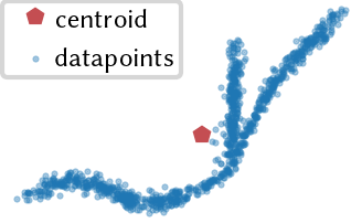
Three plots are shown in this figure. The first plot shows the data points of a Y-shaped cluster. The cluster’s weighted average data point is indicated. The second plot shows the same cluster’s data points coloured by the points’ centrality. The third plot shows three thresholded versions of the cluster centrality graph where increasingly more eccentric edges are removed, indicating how branches separate and become detectable as clusters.

Algorithm 1 A high-level overview of the FLASC algorithm.

1:function flasc($\mathbf{X},d$)

2:$\triangleright$ $\mathbf{X}$ is a dataset with $N$ feature vectors $\mathbf{x}_{(\cdot)}$ and $d$ is a distance metric $d(\mathbf{x}_{i},\mathbf{x}_{j})$.

3:     evaluate hdbscan($\mathbf{X},d$) and store its internal data structures.

4:     for each detected cluster $C_{j}$ do

5:         compute the centrality $c(\mathbf{x}_{i})$ for all $\mathbf{x}_{i}\in Cj$.

6:         extract the cluster centrality graph $\mathbf{G}_{c}^{C_{j}}$.

7:         compute the Single Linkage Clustering hierarchy of $\mathbf{G}_{c}^{C_{j}}$

8:         simplify the clustering hierarchy using a minimum branch size $m_{b}$.

9:         extract labels and probabilities for a ‘flat’ clustering.

10:     end for

11:     combine the cluster and branch labels and probabilities.

12:     return the membership labels and probabilities.

13:end function

Detecting flares in a cluster centrality graph $\mathbf{G}_{c}^{C_{j}}$ is conceptually similar to detecting density-based clusters. Instead of the density profile (as in Figure 2), we now look at the eccentricity profile ($e(\mathbf{x}_{i})=1/c(\mathbf{x}_{i})$). The contour clusters in this profile correspond to the flares we want to detect. Effectively, we perform Single Linkage Clustering (Sibson, 1973) on the cluster centrality graph $\mathbf{G}_{c}^{C_{j}}$ using a Union-Find data structure as in (McInnes and Healy, 2017). The resulting hierarchy is simplified using a minimum branch size $m_{b}$.

HDBSCAN*’s ‘flat’ clustering strategies are used to compute branch labels and membership probabilities from these condensed hierarchies. Points that enter the filtration after the selected flares have connected—i.e. points with the noise label—are given a single non-noise label representing the cluster’s centre. Finally, the cluster and branch labels are combined (see Figure 1). By default, points in clusters with two or fewer branches are given a single label because two branches are expected in all clusters, indicating the outsides growing towards each other. The label sides as branches parameter can be used to turn off this behaviour and separate the ends of elongated clusters in the labelling. The cluster and branch probabilities are combined by taking their average value (see Figure 4).

Other labelling and probability combinations are possible. For example, the cluster and branch probability product more strongly emphasises the outsides of the flares (see Figure 4). Like McInnes et al.’s HDBSCAN* implementation (McInnes et al., 2017), FLASC supports computing flare membership vectors, describing how much a point $\mathbf{x}_{i}\in C_{j}$ belongs to each branch $B_{b}\subset C_{j}$. These membership values are based on the geodesic distances in the cluster approximation graph $\mathbf{G}_{k}^{C_{j}}$: $d_{geo}(\mathbf{r}_{B_{b}},\mathbf{x}_{i})$, where $\mathbf{r}_{B_{b}}$ is the branch’ root, i.e., the point closest to the branch’s weighted average $\bar{\mathbf{x}}_{B_{b}}$, where the probability assigned to each point is used as weight. The flare membership vectors can be used to label points by the closest branch root, as in Figure 4, which can change the label for central points. Alternatively, a softmax function can be used to convert $d_{geo}(\mathbf{r}_{B_{b}},\mathbf{x}_{i})$ into the membership probabilities:

(4) $$p(\mathbf{x}_{i},B_{b})=\frac{e^{c_{b}(\mathbf{x}_{i},B_{b})}}{\sum_{B_{l}\in C_{j}}{e^{c_{b}(\mathbf{x}_{i},B_{l})}}},$$

where $c_{b}(\mathbf{x}_{i},B_{b})$ converts $d_{geo}(\mathbf{r}_{B_{b}},\mathbf{x}_{i})$ into a flare centrality as in (3) (see Figure 4).

Low persistent branches can be ignored using a branch selection persistence parameter, analogous to HDBSCAN*’s cluster selection epsilon (Malzer and Baum, 2020). However, flares do not have to start at zero centrality, so branch selection persistence describes the minimum centrality range rather than a single centrality threshold value. The procedure for applying this persistence threshold evaluates selected branches in increasing order of persistence to avoid parent-child relations in the final chosen branches. In addition, the flare membership probability is based on the flare’s maximum eccentricity rather than the selected segment’s maximum eccentricity in the branch condensed tree, as is used for clusters.

Figure 4. Different ways to combine cluster and branch membership probabilities. The cluster and branch probability average (a) and product (b) are visualised with desaturation. (c) Points labelled by the geodesically closest branch root—i.e., the point closest to the branch’s weighted average—and desaturated as in (a). (d) Weighted branch membership for the orange branch is visualised by transparency. Branch memberships are computed from the traversal distance to the branch’s root.

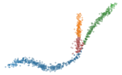
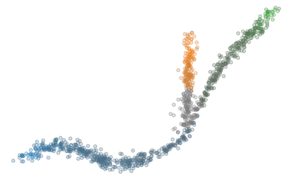
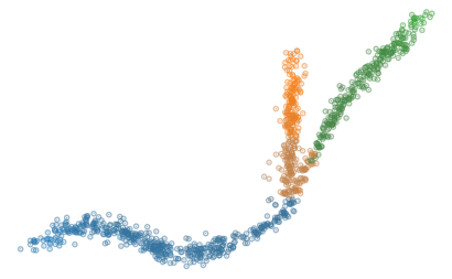
Four scatterplots of a Y-shaped cluster with different cluster and branch labelling and probability combinations.

3.2. Stability

Two notions of stability are relevant: (1) the algorithm has to provide similar results when run repeatedly on (different) samples of an underlying distribution, and (2) the detected branch hierarchies have to represent the clusters’ underlying topology accurately.

Vandaele et al. analysed the latter notion of stability for graph-based branch detection, explaining that the graph approximation should accurately represent the underlying shape and the graph-based centrality function should accurately describe the points’ centrality in a cluster’s metric space $(C_{j},d_{mreach})$. For the normalised centrality used by Carlsson (Carlsson, 2014), they showed that the bound on the bottleneck distances between true and empirical persistence diagrams is tight if the metric distortion induced by the graph and its maximum edge weight is small.

Both the full and core cluster approximation graph used by FLASC satisfy the low maximum edge weight requirement as their largest edge weight is the minimum mutual reachability distance required for all points in the cluster to be connected in the graph. Additionally, the metric distortion should be small as only edges in the local neighbourhood of data points are included because the clusters do not contain noise points.

The centrality metric (Equation (3)) is more complex to analyse. It is a $\mathrm{c}$-Lipschitz-continuous function when considered over the cluster centrality graph’s edges:

$$|\max{\{c(\mathbf{x}_{i}),c(\mathbf{x}_{j})\}}-\max{\{c(\mathbf{x}_{k}),c(\mathbf{x}_{l})\}}|\leq\mathrm{c}\;d_{mreach}(\mathbf{x}_{i},\mathbf{x}_{l}),$$

where $\mathrm{c}$ is a constant describing the continuity, $(\mathbf{x}_{i},\mathbf{x}_{j})\in\mathbf{G}_{c}^{C_{j}}$ and $(\mathbf{x}_{k},\mathbf{x}_{l})\in\mathbf{G}_{c}^{C_{j}}$, and the mutual reachability between $\mathbf{x}_{i}$ and $\mathbf{x}_{l}$ is the largest of the four points. However, the position of the cluster’s centroid $\bar{\mathbf{x}}_{C_{j}}$ influences how well the function represents the centrality in the cluster’s metric space $(C_{j},d_{mreach})$. We aim to show the current approach strikes a good balance between computational cost and stability in the experiments presented in Section 4.

3.3. Complexity

The algorithm’s most computationally expensive steps are constructing the full cluster approximation graphs and computing the cluster centrality graphs’ single linkage hierarchies. Naively, the worst-case complexity for creating a cluster approximation graph is $\mathcal{O}(n_{c}^{2})$, where $n_{c}$ is the number of points in the cluster. Usually, the average case is much better because the approximation graphs rarely are fully connected. After all, HDBSCAN*’s noise classification limits the density range within the clusters. Furthermore, the space tree that we re-use from the HDBSCAN* clustering step provides fast asymptotic performance for finding the graph’s edges. The exact run-time bounds depend on the data properties. They are challenging to describe (as explained in (McInnes and Healy, 2017)), but an average complexity proportional to $\mathcal{O}(n_{e}\log{N})$ is expected, where $n_{e}$ is the number of edges in the graph. Computing single linkage hierarchies from the cluster centrality graphs is possible in $\mathcal{O}(n_{e}\alpha(n_{e}))$ using McInnes et al. (McInnes et al., 2017)’s Union-Find implementation adapted to ignore edges between data points that are already in the same connected component. Like McInnes and Healy (McInnes and Healy, 2017), we feel confident that FLASC achieves sub-quadratic complexity on average, which we demonstrate in a practical example in Section 4.4.

4. Experiments and Results

This section presents two case studies demonstrating how FLASC can be used on real-world data to detect branch-based subgroups. In addition, we describe two analyses of synthetic data sets to demonstrate FLASC’s stability and computational performance.

4.1. Case Study: Diabetes Types

In 1979, Reaven and Miller (Reaven and Miller, 1979) collected and analysed a data set about diabetes patients. Previously, they had found a “horse shoe”-shaped relation between glucose levels and insulin responses in diabetes patients (Reaven and Miller, 1979). Their 1979 paper attempted to clarify that relationship by measuring additional metabolic variables. Three of those variables turned out to be very informative in a 3D scatterplot. Our recreation of that scatterplot is shown in Figure 5(a), illustrating a dense core with two less-dense branches, which Reaven and Miller considered unlikely to be a single population (Reaven and Miller, 1979).

More recently, Singh et al. used the data set to demonstrate how Mapper with a density-based lens function visualises these flares without manually specifying which dimensions to plot (Singh et al., 2007). Their analysis leverages the flares’ lower density, allowing them to be detected without a centrality metric. In general, though, local density minima do not always relate to branches, especially for data sets with multiple branching clusters.

In this section, we show how FLASC can detect the branching pattern in this data set and classify the observations by their branch without manually extracting the flares from a visualisation.

4.1.1. Evaluation and settings

The data set—obtained from (Andrews and Herzberg, 1985)—contains five variables describing 145 subjects: the relative weight, the plasma glucose level after a period of fasting, the steady-state plasma glucose response (SSPG), and two areas under a curve—one for glucose (AUGC) and one for insulin (AUIC)—representing the total amount observed during the experimental procedure described in (Reaven and Miller, 1979). All five variables were z-score normalised and used to compute the Euclidean distance between subjects.

Both FLASC and HDBSCAN* were evaluated on the normalised data set. FLASC was tuned to find a single cluster with multiple branches by setting min samples $k=5$, min cluster size $m_{c}=100$, min branch size $m_{b}=5$, and enabling allow single cluster. HDBSCAN* was tuned to find multiple clusters with min samples $k=5$ and min cluster size $m_{c}=10$.

4.1.2. Results

(a) Illustration

(b) FLASC

(c) HDBSCAN*

Figure 5. (a) A three-dimensional scatterplot showing the area under the plasma glucose curve (AUGC), the area under the insulin curve (AUIC), and the steady state plasma glucose response (SSPG) as described by (Reaven and Miller, 1979). (b) FLASC’s classification tuned to find one cluster with multiple branches. One low-persistent branch (blue) corresponding to the bottom of the centre could be filtered out by specifying a persistence threshold. (c) HDBSCAN*’s labels tuned to find multiple clusters. Grey points were classified as noise.

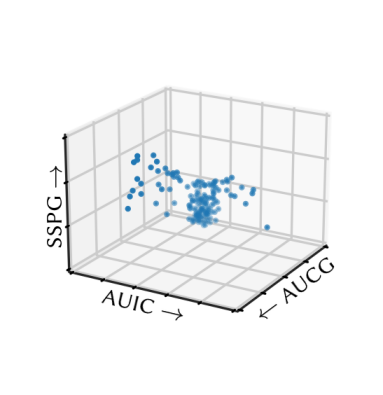
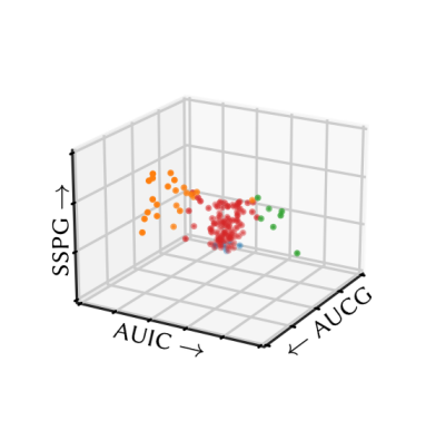
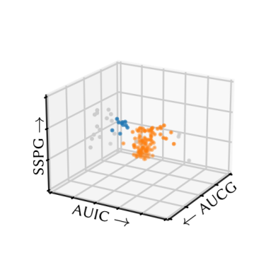
Three variants of the 3D scatterplot indicating how the subgroups that HDBSCAN* and FLASC detect relate to Reaven and Millers interpretation.

Figure 5 shows the resulting classifications encoded as colour on the 3D scatterplot. FLASC’s classification (Figure 5(b)) distinguishes the flares from the central core. The algorithm also finds a low-persistent flare representing the central core’s bottom. This flare could be ignored by specifying a persistence threshold. In contrast, as expected, HDBSCAN*’s classification (Figure 5(c)) does not find the flares. Instead, it finds part of the left flare as a small low-persistent cluster and merges most of the right flare with the central core. This demonstrates that branching structures cannot be detected as density-based clusters when they do not contain local density maxima. In this case, though, specifying a larger minimum cluster size and re-clustering the points classified as noise should detect the two branch-based subgroups because these branches have a lower density than the central core.

All in all, this case study demonstrated how FLASC detects branch-based subgroups that do not contain local density maxima without having to specify the relevant features in advance or extract the subgroups visually. Practically, FLASC would have made it easier for researchers to detect the three groups in this data set, which was relevant for understanding diabetes and its causes.

4.2. Case Study: Cell Development

The small roundworm C. Elegans is often used in biological studies and was the first animal to have its genome sequenced completely (elegans Sequencing Consortium*, 1998). More recently, Packer et al. analysed gene expressions in C. Elegans embryos through single-cell RNA sequencing to uncover the trajectories along which cells develop (Packer et al., 2019). Broadly speaking, this data set describes what happens in cells as they develop from a single egg cell into all the different tissues within fully grown C. Elegans worms.

After pre-processing, the data set appears to contain both cluster and branching structures when viewed in Packer et al.’s 3D projection (Packer et al., 2019). In this case study, we demonstrate that FLASC can provide additional information about a data set’s structure even when the main subgroups can be detected as clusters. This information, however, is limited to the most eccentric connections between branches.

4.2.1. Evaluation and settings

The data and pre-processing scripts were obtained from Monocle 3’s (Cao et al., 2019) documentation (Pliner et al., 2022). The pre-processing stages normalise the data, extract the 50 strongest PCA components, and correct for batch effects using algorithms from (Haghverdi et al., 2018). HDBSCAN* and FLASC were evaluated on the pre-processed data using the angular distance metric because neither algorithm supports the cosine distance metric in their optimised code paths. HDBSCAN* was tuned to find multiple clusters with min samples $k$ and min cluster size $m_{c}$ set to $20$. FLASC was tuned to find a single cluster by selecting min samples $k=5$, min cluster size $m_{c}=20$, min branch size $m_{b}=20$, enabling allow single cluster, and setting cluster selection epsilon to $1/1.4$ to classify points as noise if they are ‘too far away’ from the clusters. Branches were detected using the core cluster approximation graph.

4.2.2. Results

Figures 6(a) and 6(b) show the pre-processed data projected into two dimensions using densMAP (Narayan et al., 2021). Data points are coloured to indicate the detected flares and clusters, respectively. In Figure 6(a), the core cluster approximation graph’s edges are also drawn. Notice how some parts of the projection are not connected as one might assume from their coordinates. For example, there are edges between branches 1 and 5 and branches 12 and 14.

(a) FLASC

(b) HDBSCAN*

(c) Branch hierarchy

(d) Cluster hierarchy

Figure 6. 2D densMAP (Narayan et al., 2021) projections of the 50 dimensional pre-processed single-cell gene expression data from (Packer et al., 2019) coloured by the detected branches (a) and clusters (b). (c) and (d) show the branch and cluster condensed trees as icicle plots adapted from (McInnes et al., 2017). The selected branches and clusters are indicated with numbers and coloured. The cluster approximation graph’s edges are drawn on top of the 2d projection in (a).

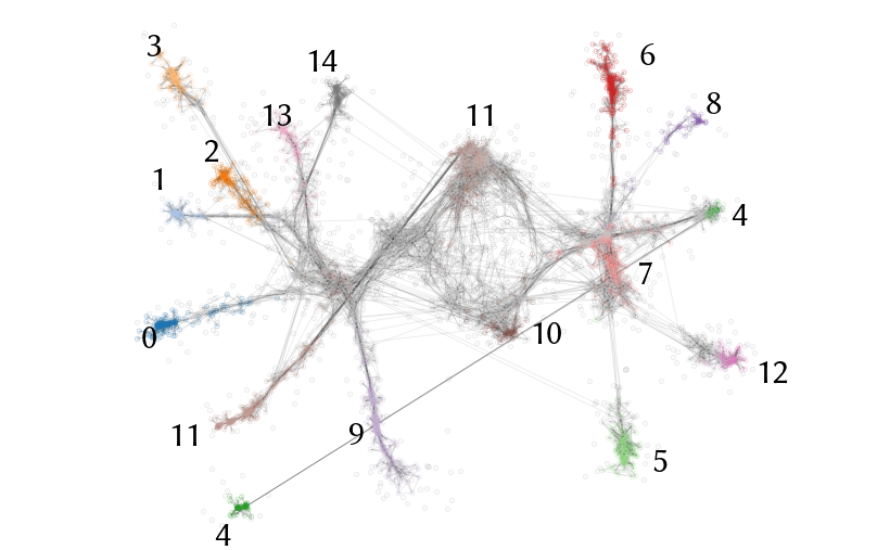
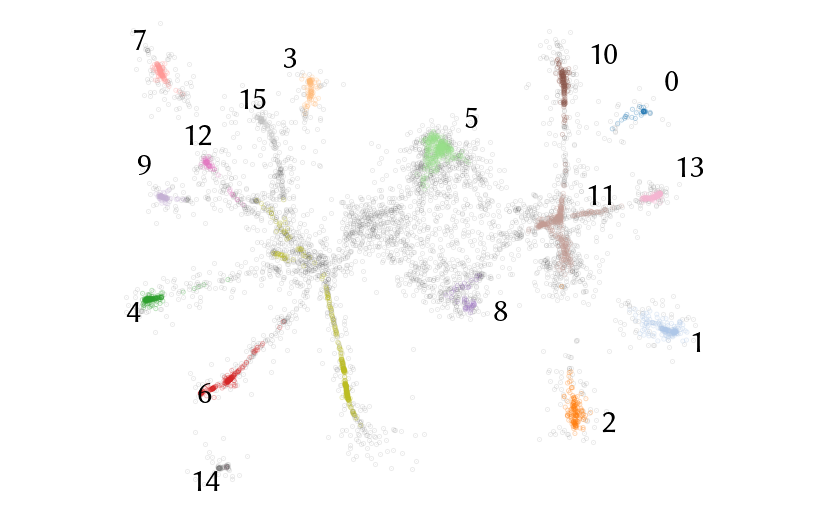
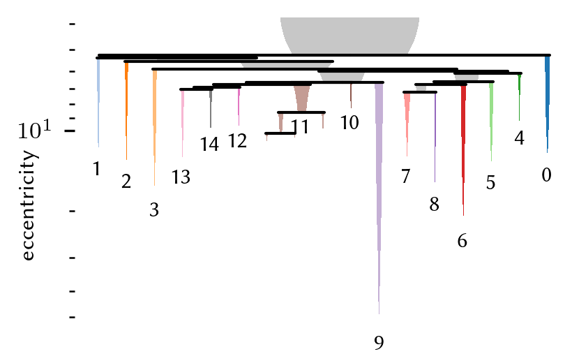
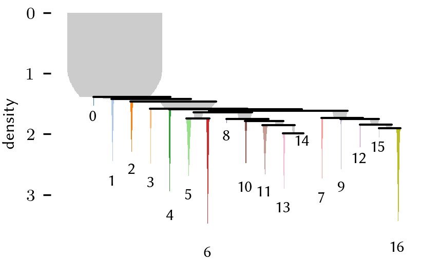
The clusters that HDBSCAN* and branches that FLASC detect on the single-cell sequencing data. The cluster and branch hierarchies partially communicate the point cloud’s shape.

Figures 6(c) and 6(d) visualise the branch and cluster condensed trees, respectively, using an icicle plot adapted from McInnes et al. (McInnes et al., 2017). Segment widths encode the number of points in the tree below the segment. Numbers and colours indicate the selected branches and clusters.

In contrast to the previous case study, HDBSCAN* appears to detect all flares as clusters, indicating that the branches have a local density maximum. Considering that the branches correspond to cell fates—i.e., the developmental end-states—it is unsurprising that local density maxima occur within them. One could imagine that the variation in gene expression is higher during development and that fully developed cells are observed more frequently. Both scenarios could cause these local density maxima. HDBSCAN* also classifies a lot of points as noise. Consequently, it does not capture the trajectories: it only detects the subgroups and does not provide information about how they relate. For example, clusters 5 and 6 are neighbours in the cluster-condensed tree (Figure 6(d)), but the trajectory between those clusters would pass through cluster 16.

FLASC finds the same subgroups, except that clusters 5 and 6 are combined into branch 11 and clusters 13 and 15 into branch 4. In addition, the branch condensed tree (Figure 6(c)) captures (some of) the cluster’s shape. Branches that merge into the cluster near each other are also close in the branch-condensed tree. See, for example, branches 6 and 8. For branches connected to multiple other branches in the cluster approximation graph, only the most eccentric connection is captured by the branch-condensed tree. For example, branches 12 and 14 are neighbours in the hierarchy, while their connections to other branches are more apparent in the densMAP projection (Figure 6(a)).

All in all, this case study demonstrated that FLASC’s branch hierarchy can provide information about a cluster’s shape that may not be obvious in 2D projections.

4.3. Flare Stability

In this section, we explore FLASC’s stability in terms of its difference in output on multiple samples of the same underlying distribution and its accuracy compared to a ground truth.

4.3.1. Datasets

For this comparison, two-dimensional data sets containing a single cluster with $3$ branches laid out as a three-pointed star were generated (Figure 7). The branches span from the centre outwards and are spread out equally across the $2$D plane—i.e., the angle between adjacent branches is $120$ degrees. Each branch has a length $b_{l}$ and contains $100$ points exponentially spaced from the inside out. Consequently, the density is highest at the cluster’s centre and lowest in the branch ends, and this difference increases with the branch length. Normally distributed noise ($\mu=0$) is added to the points’ coordinates using a noise ratio parameter $n_{r}$ to determine the distribution’s standard deviation $\sigma$:

(5) $$n_{r}=\frac{4\sigma}{\sqrt{\frac{1}{2}}b_{l}}.$$

Here, $n_{r}$ indicates that approximately $95\%$ of the sampled noise values fall within $\pm\sqrt{\frac{1}{2}}n_{r}b_{l}$ of zero. Consequently, approximately $90\%$ of points are moved less than $n_{r}b_{l}$ from their original 2D position. By design, the branches do not reliably contain local density maxima, making them practically undetectable as density-based clusters (see Figure 11).

4.3.2. Evaluation and settings

The data sets were sampled with varying branch lengths $b_{l}$ ($2$ to $100$ in $10$ exponentially spaced steps) and noise ratios $n_{r}$ ($0$ to $1$ in $10$ exponentially spaced steps). Ten data sets were sampled for each parameter combination, resulting in $1000$ point clouds (see Figure 8 for one example of each combination). FLASC was evaluated with full and core approximation graphs on each data set, allow single cluster enabled, min samples $k=5$, min cluster size $m_{c}=25$, a varying min branch size $m_{b}$ ($2$ to $24$ in steps of $2$), and both the eom and leaf branch selection strategies.

For each evaluation, the resulting data point labels and probabilities were stored. From these values, we computed the Adjusted Rand Index (ARI) (Hubert and Arabie, 1985) to describe the agreement between ground truth and assigned partitioning labels adjusted for chance. In addition, for each subgroup detected by FLASC, we computed the weighted average coordinates—i.e., found centroids—to describe the algorithm’s stability. These centroids were assigned to the closest ground truth centroid, and their (unweighted) average position was computed for each ground truth group over the $10$ data sets with the same branch length $b_{l}$ and noise ratio $n_{r}$. The distances between the centroids and their (unweighted) average normalised by the branch length $b_{l}$ serve as a stability metric referred to as the centroid spread (see Figure 7).

Finally, we selected the parameter values that maximised the average ARI and minimised the average centroid spread over all data sets. These parameter values were: min branch size $m_{b}=12$, the full cluster approximation graph, and eom branch selection strategy.

Figure 7. An illustration explaining the centroid spread stability metric. (a) A single point cloud with branch length $b_{l}=65$ and noise ratio $n_{r}=0.852$ coloured by the ground truth labels. The average position per ground truth label—i.e., true centroid—is indicated by black crosses: one for each branch and one for the entire cluster. (b) The weighted average position of each subgroup detected by FLASC—i.e., found centroids—for all $10$ data sets with these parameters coloured by the closest true centroid. (c) The unweighted average found centroid positions per subgroup shown as black pentagons. The centroid spread is quantified by the distances from the centroids to this root position normalised by the branch length $b_{l}$. Consequently, the metric describes stability, not accuracy.

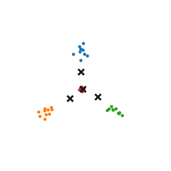
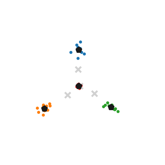
A visual explanation of the centroid spread stability metric.

4.3.3. Results

Figure 8. Data sets with varying noise ratios and branch lengths coloured by the FLASC labels. Notice that the central subgroup in red increases with the noise ratio. Branch lengths (columns) are normalised visually.

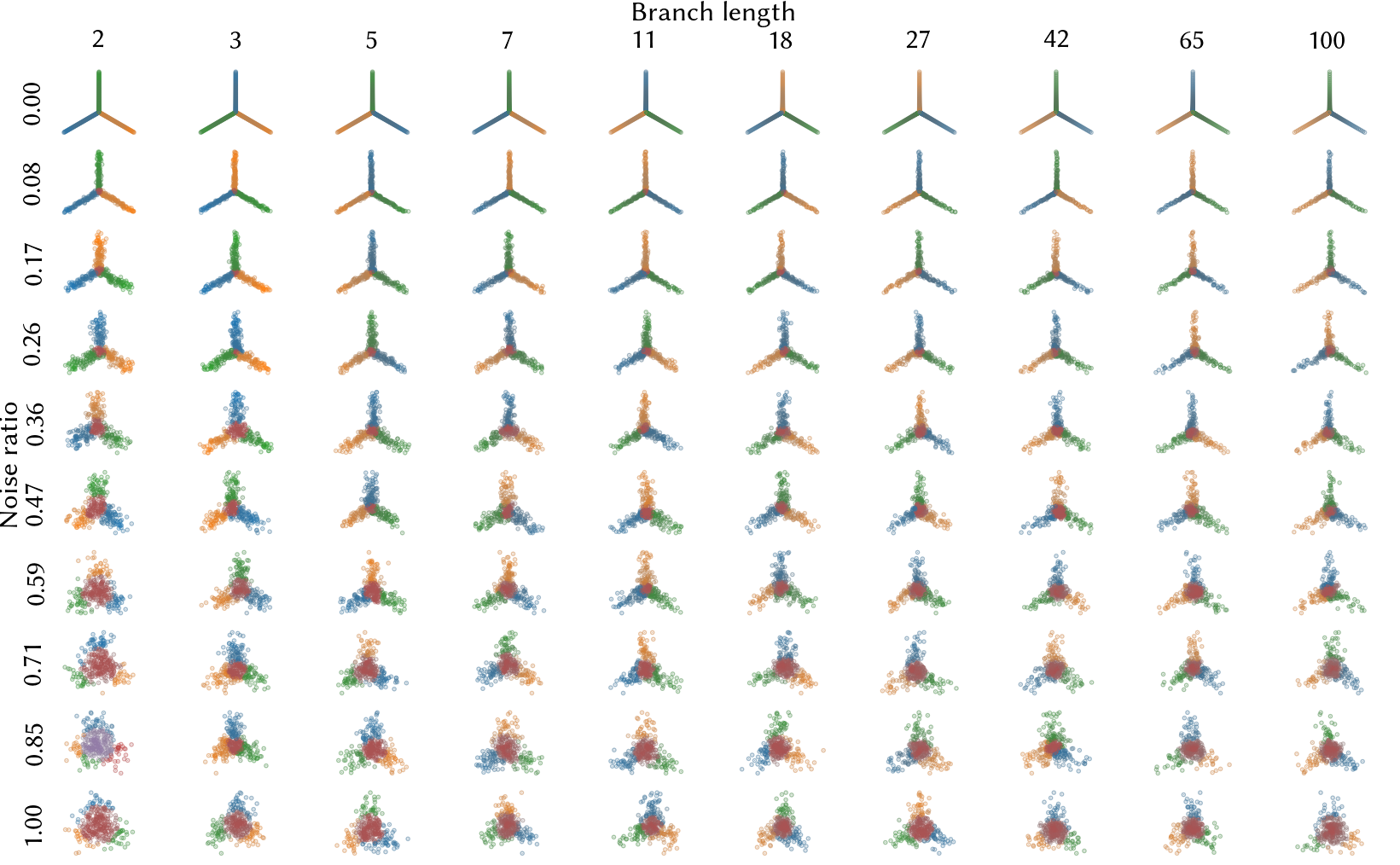
Scatterplots for the tree-pointed star point clouds for all branch length and noise ratio combinations with FLASC’s labelling indicating that FLASC detects the branches as a single subgroup in almost all combinations.

Figure 9. Heatmaps showing FLASC’s (a) average Adjusted Rand Index (ARI) and (b) $95$th percentile centroid spread over $10$ point-clouds generated with noise ratio $n_{r}$ and branch length $b_{l}$. The centroid spread distances were normalised with the branch length $b_{l}$, allowing for comparison between data sets with different parameters.

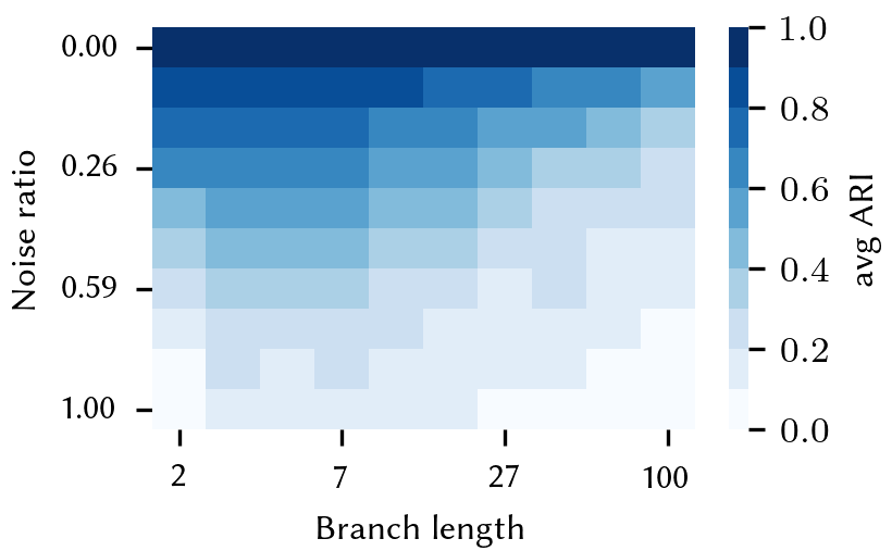
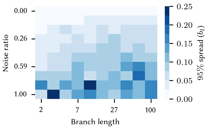
Two heatmaps indicating for which branch lengths and noise ratios FLASC performs well.

Figure 8 shows one data set for each branch length $b_{l}$ and noise ratio $n_{r}$ combination, where the data points are coloured by their FLASC labels. As expected, FLASC detected the three branches and the cluster’s centre in almost all data sets. This pattern was consistent across all $10$ data sets generated for each branch length $b_{l}$ and noise ratio $n_{r}$ combination, as shown by the average ARI value heatmap in Figure 9. This latter figure indicates that FLASC’s average ARI decreases as the noise ratio increases, which can be explained by an increasing number of points assigned to the centre label. While this centre label makes sense semantically, it is not present in the ground truth labels. Therefore, the ARI value is expected to decrease as more points are given the centre label. For this reason, it could be argued that the ARI values give a too-pessimistic view of FLASC’s performance on this data set.

FLASC’s stability was analysed through its centroid spread over different data set samples with the same branch length $b_{l}$ and noise ratio $n_{r}$. Figure 9 visualises the $95$th percentile of the centroid spread distances as a heatmap. In general, the centroid spread was relatively low, with the $95$th distance percentile being less than $\frac{1}{8}b_{l}$ in most of the evaluated noise ratio–branch length space. All in all, these values demonstrate that FLASC produces a similar output on data set samples with the same underlying distribution.

4.4. Computational Performance

In this section, we explore how the computational cost of FLASC compares to other clustering algorithms. Given the challenges in accurately benchmarking the computational performance of algorithms (Kriegel et al., 2017), we limit this comparison to the trends in run time scaling over data set size and number of dimensions for specific implementations.

4.4.1. Datasets

A Gaussian random walk process was used to generate data sets for the performance comparison. Specifically, for a space with $d$ dimensions, $c$ uniform random starting points were sampled in a volume that fits five times the number of to-be-generated clusters. Then, $5$ random walks, with $50$ steps each, were sampled from each starting point. Every step moved along one of the dimensions with a length sampled from a normal distribution ($\mu=0$, $\sigma=0.1$). The resulting point clouds have more varied properties than the Gaussian blobs McInnes and Healy (McInnes and Healy, 2017) used for their run time comparison of HDBSCAN*, including non-trivially varying densities and branching patterns within clusters. Note that the number of (density-based) clusters in each point cloud may differ from the number of starting points $c$ due to possible overlaps or sparse regions in the random walks.

4.4.2. Evaluation and settings

The random walk data sets were generated with varying numbers of dimensions ($2$, $8$, $16$) and starting points ($2$ to $800$ in $10$ exponentially spaced steps). $10$ data sets were sampled for each combination of parameters, resulting in a total of $300$ point clouds.

Three clustering algorithms’ Python implementations were compared: fastcluster (Müllner, 2013) (version 1.1.26), McInnes and Healy’s HDBSCAN* (McInnes et al., 2017) (version 0.8.28), and FLASC with the full and core approximation graphs. HDBSCAN* and both FLASC versions were evaluated with min samples $k=10$, min cluster size $m_{c}=100$, min branch size $m_{b}=20$, allow single cluster enabled, and their multiprocessing support disabled to better describe the algorithms’ intrinsic complexity. Fastcluster’s default parameter values were used, resulting in a single linkage dendrogram.

Time measurements were performed on a computer with a $3.4$GHz Intel Core i7-6700 processor and $16$GB RAM. Each algorithm was evaluated on each data set once, recording the run time and number of detected clusters. The smallest data set for which an algorithm required more than $80$ seconds was recorded for each number of dimensions. Larger data sets were not evaluated for those algorithms.

(a) 2D

(b) 8D

(c) 16D

Figure 10. Average run time in seconds over $10$ random walk point clouds with (a) 2 dimensions, (b) 8 dimensions, and (c) 16 dimensions. The shaded areas around each line indicate the mean’s $95\%$ confidence interval. Note the changes in the $y$ range between the sub-figures.

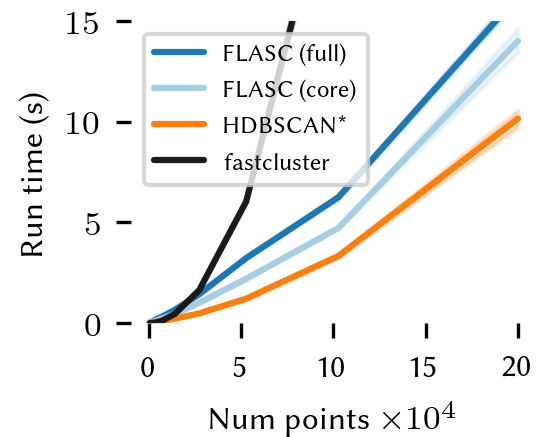
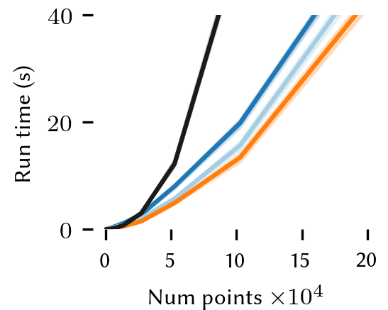
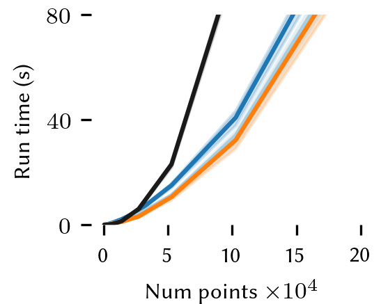
Three line plots indicating the average run times of fastcluster, HDBSCAN*, and the two FLASC variants for random walk data sets with 2, 8, and 16 dimensions.

4.4.3. Results

Figure 10 shows the algorithms’ average run times in seconds over the data set size and number of dimensions. There are three patterns of note: firstly, fastcluster shows a quadratic trend, resulting in the longest run times. The other algorithms show sub-quadratic trends on the $2$ and $8$ dimensional data sets but approach fastcluster’s quadratic trend in the $16$ dimensional case. This is expected because constructing and querying space trees becomes more expensive with more dimensions. Secondly, HDBSCAN* and both FLASC variants scale similarly in all three conditions. HDBSCAN* is consistently the fastest of the three, followed by FLASC with the core approximation graph. However, their run time differences diminish in the higher dimensional cases, indicating that the additional cost of branch detection is relatively low compared to the cost of detecting the clusters.

In conclusion, both FLASC variants’ computational performance scale similarly to HDBSCAN* and the more dimensions the data contains, the smaller the scaling trend differences between the algorithm.

5. Discussion

Two case studies on real-world data and two analyses on synthetic data were performed to demonstrate FLASC and its properties. Section 4.1 showed how the flare-detection post-processing step enabled the detection of subgroups representing two diabetes types. Section 4.2 showed a more complex data set in which the subgroups are detectable by both FLASC and HDBSCAN*. FLASC still provides a benefit for exploration because the uncovered branch hierarchy includes information about the connectivity between the subgroups. However, structure learning algorithms—such as Reversed Graph Embeddings (Mao et al., 2017) and Bonnaire et al.’s mixture model approach (Bonnaire et al., 2022)—can provide even more information about the data’s shape at more computational costs. Section 3.2 demonstrated FLASC’s stability by showing that its output is similar on multiple samples of the same underlying distribution. This analysis could be expanded to investigate how well FLASC deals with shapes with unequal branch lengths. The weighted average data point—and centrality metric as a result—may not accurately reflect the centre of such clusters. Consequently, FLASC’s branch hierarchy will be a less accurate representation of the underlying topology but should still detect the flares. Monocle 3 (Qiu et al., 2017) deals with this problem by selecting the centre point in a projection manually (Pliner et al., 2022). Section 4.4 demonstrated that FLASC’s computational performance scales similar to HDBSCAN*. The scaling trends appeared to become more similar as the data contained more dimensions. However, neither algorithm was evaluated with multiprocessing enabled, which can introduce run-time differences in practical applications. In addition, extracting the full cluster approximation graph can be more expensive than reported, depending on the data’s characteristics.

5.1. Branch-detection’s practical value

As briefly mentioned in Section 1.2, the argument that branches are not detectable as clusters only applies when they do not contain local density maxima. In other cases, the subgroups can be detected as density-based clusters. If one is only interested in the existence of subgroups, then there may not be many data sets where FLASC provides a benefit over HDBSCAN*, as relevant (sparse) subgroups may be rare, and HDBSCAN*’s assumption that such points are noise may be valid. However, FLASC provides a benefit when looking for patterns in the relatively uncommon parts of a data set or when the cluster’s shapes are relevant. The algorithm, therefore, is not the default go-to solution for all things clustering. Instead, we envision it as a valuable tool for exploring unfamiliar data, providing guidance into which subpopulations exist and informing follow-up questions. Knowing that a cluster may represent multiple subgroups can be very relevant.

5.2. Alternative centrality metrics

The presented FLASC algorithm uses a geometric distance-to-centroid centrality metric to describe how central data points lie within a cluster (Figure 3, Equation 3). An interesting alternative is a geodesic centrality, which measures the number of edges between each data point and the cluster’s root point in the cluster approximation graph. Here, the root point can be chosen as the data point closest to the cluster’s centroid, as we did for the branch-membership vectors in Section 3.1 (Figure 4). This geodesic centrality would agree with the notion that distances in high dimensional data may not accurately reflect distances along the intrinsic structure of a data set, which was one of the motivations for Reversed Graph Embeddings (Mao et al., 2017). It would also be closer to the maximum shortest-path centrality metric used by Vandaele et al. (Vandaele et al., 2021).

Several trade-offs between the geometric and geodesic centrality metrics made us choose the geometric one. (1) Computing the geodesic centrality is more expensive because it requires an additional traversal over the entire cluster approximation graph. The extra cost, however, should be low compared to other parts of the algorithm. (2) The resolution of the geodesic centrality is lower, as it expresses the number of edges to the root point. As a result, zero-persistent branches are more likely to occur. In addition, it reduces the detectability of small branches that are well connected. On the other hand, that can be seen as beneficial noise suppression. In addition, the branch selection persistence parameter becomes more interpretable and would represent the traversal depth of a branch in the approximation graph. (3) The cluster’s centroid may lie outside of the cluster itself, resulting in a root point and centrality values that do not accurately describe its centre. For example, imagine a U-shaped cluster. The centroid would lie in between the two arms, and the root would lie in one of the arms. As a result, the geodesic metric would find one smaller and one larger branch rather than two equal branches. On the other hand, the geometric centrality finds the two branches and the connecting bend as three separate groups. Confusingly, it also contains two regions with a local centrality maximum, which FLASC gives a single label.

FLASC’s general process can also be used with metrics that capture other aspects than data points’ centrality. At its core, FLASC consists of two filtrations, one to determine the connectivity between data points and one to analyse a signal on the resulting graph. The process would then describe how many distinct local minima (or maxima) of the metric exist within the clusters. The resulting interpretation does not have to relate to the cluster’s shape.

One could even interpret FLASC as two applications of HDBSCAN*: one over the density and one over the eccentricity. This perspective raises a possible improvement to the algorithm by translating the mutual reachability concept to the centrality metric. The idea of ‘pushing away points in low-density regions’ can also be applied to the centrality and would emphasise the centrality difference between the centre and branch ends. Additionally, smoothing the centrality profile by incorporating neighbouring values could improve the algorithm’s robustness to noise. The additional computational cost should be low, as points’ neighbours are already known when the centrality is computed. Another way to improve noise robustness could be to implement the mutual $k$-nearest neighbour approach used by Dalmia and Sia (Dalmia and Sia, 2021) to improve UMAP projections. It would provide a subgraph of the core approximation graph that better reflects the cluster’s connectivity in high dimensional data sets. We leave evaluating these ideas for future work.

5.3. Visually summarising data’s shape

A strength of Mapper (Singh et al., 2007) and Reversed Graph Embeddings (Mao et al., 2017) is that they can summarise the data’s shape using intuitive visualisations. While FLASC’s branch-condensed tree provides some information about the clusters’ shapes, interpreting the cluster’s shape from it is not trivial. Practically, this means that detecting branch-based subgroups is simple, but interpreting trajectories or shapes is difficult. For example, in Section 4.2, some connections in the branch hierarchy (Figure 6(c)) are not apparent from the 2D densMAP (Narayan et al., 2021) projection (Figure 6(a)). However, such 2D projections should not be interpreted as a canonical representation of the data’s shape, as they do not necessarily retain the data’s local and global structures (Chari et al., 2021).

Studying how well two-dimensional layouts of FLASC’s cluster approximation graphs work as shape summarising visualisations would be an interesting future research direction. These graphs directly encode the connectivity used by the algorithm. Therefore, explicitly drawing their edges avoids the visual conflicts we found with the densMAP projections. Another benefit is that all (non-noise) data points are represented in the graphs once. Directly visualising the graphs, however, probably does not scale to larger sizes in terms of computational cost for the layout algorithm and visual interpretability. Ways to summarise the networks would have to be found, which could be based on $k$-means centroids like in Reversed Graph Embeddings or the local density maxima in the cluster.

6. Conclusion

We presented the FLASC algorithm that combines HDBSCAN* clustering with a graph-based branch-detection approach. We have shown that the algorithm can detect flare-based subgroups that do not contain local density maxima in real-world data without specifying features of interest or extracting the flares from a visualisation manually. In addition, we demonstrated that the branching hierarchy, as found by FLASC, can provide information about a cluster’s shape that is not present in HDBSCAN*’s output when the subgroups are detectable as clusters. Two analyses of synthetic data showed that FLASC provides similar results for samples of the same underlying distribution and that its computational performance scales similarly to HDBSCAN*.

Appendix A HDBSCAN* on branch stability data

Section 4.3.1 briefly mentioned that the data sets used for the stability analysis were designed so that the branches do not contain local density maxima. This section shows which subgroups HDBSCAN* detects on those data sets. HDBSCAN* was tuned with min samples $k=5$, min cluster size $m_{c}=8$, and the leaf cluster selection strategy. The parameters were selected using the procedure described in Section 4.3.1. Figure 11 shows the resulting classifications. Notice that subgroups are found within the branches, but the branches are not described by a single subgroup. In addition, many points are classified as noise by HDBSCAN*.

Figure 11. The data sets with varying noise ratios and branch lengths from Section 4.3 coloured by HDBSCAN*’s classification when tuned to detect multiple clusters. Branch lengths (columns) are normalised visually.

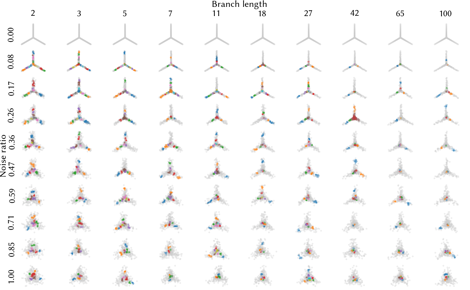
This figure shows the tree-pointed star point clouds for all branch length and noise ratio combinations with HDBSCAN*’s labelling indicating that it does not detect the branches as a single subgroup.