Policy Learning with Distributional Welfare

Abstract

In this paper, we explore optimal treatment allocation policies that target distributional welfare. Most literature on treatment choice has considered utilitarian welfare based on the conditional average treatment effect (ATE). While average welfare is intuitive, it may yield undesirable allocations especially when individuals are heterogeneous (e.g., with outliers)—the very reason individualized treatments were introduced in the first place. This observation motivates us to propose an optimal policy that allocates the treatment based on the conditional quantile of individual treatment effects (QoTE). Depending on the choice of the quantile probability, this criterion can accommodate a policymaker who is either prudent or negligent. The challenge of identifying the QoTE lies in its requirement for knowledge of the joint distribution of the counterfactual outcomes, which is generally hard to recover even with experimental data. Therefore, we introduce minimax policies that are robust to model uncertainty. A range of identifying assumptions can be used to yield more informative policies. For both stochastic and deterministic policies, we establish the asymptotic bound on the regret of implementing the proposed policies. In simulations and two empirical applications, we compare optimal decisions based on the QoTE with decisions based on other criteria. The framework can be generalized to any setting where welfare is defined as a functional of the joint distribution of the potential outcomes.

JEL Numbers: C14, C31, C54.

Keywords: Treatment regime, treatment rule, individualized treatment, distributional treatment effects, quantile treatment effects, partial identification, sensitivity analysis.

1 Introduction

Individuals are heterogeneous, so are their responses to treatments or programs. When designing policies (e.g., rules of allocating treatments or programs), it is important to reflect the heterogeneity of individual treatment effects. A policymaker (PM), or equivalently an analyst, would devise a policy to achieve a specific objective (e.g., welfare). Depending on how the PM aggregates individual gains, her objective can be viewed as either utilitarian or non-utilitarian. A utilitarian PM would consider welfare that takes the sum or average of individual gains to ensure the greatest benefits for the greatest number, whereas a non-utilitarian (e.g., prioritarian, maximin) PM would prioritize specific groups of individuals. The utilitarian objective has been the most widely-used criterion in the literature of treatment allocations and policy learning (e.g., Manski (2004); see below for a further review). However, there may be settings where the utilitarian goal is less sensible. For example, the target population may exhibit skewed heterogeneity (e.g., outliers). As another example, the PM may want to target a vulnerable population or privileged individuals, or a certain share of benefited individuals. The purpose of this paper is to explore objectives of a (non-utilitarian) PM who is concerned with certain aspects of the distribution (e.g., tails) of treatment effects or who has political incentives and thus makes decisions influenced by vote shares.

In this paper, we develop a policy learning framework that concerns distributional welfare. A policy is defined as a mapping from individuals’ observed characteristics to either a deterministic or stochastic decision of treatment allocation. Intuitively, the knowledge of individual treatment effects conditional on characteristics plays a crucial role in learning such a policy. We propose an objective function that is formulated based on the conditional quantile of individual treatment effects (QoTE). This objective function is robust to outliers of treatment effects and, more importantly, can reflect the PM’s level of prudence toward the target population. As quantifying the uncertainty of allocation decisions is intrinsically difficult (e.g., Chen et al. (2023)), the ability to adjust the level of prudence can be practically valuable to the PM.

Suppose the PM employs the utilitarian welfare, which can be written as a function of the conditional average treatment effect (ATE). If the policy class is unconstrained, it is optimal for the utilitarian PM to treat each subgroup (defined by observed characteristics) whenever their ATE is positive. Suppose that this PM faces a target subgroup, say black females, whose distribution of treatment effects exhibits that a small share of individuals enjoys positive treatment effects that dominate the negative effects of the remaining majority. If the resulting ATE is positive, then the PM would treat all black females, harming the majority. The objective function based on the QoTE with the quantile probability $\tau=0.5$ (i.e., the median of treatment effects) would not suffer from this sensitivity to outliers. Moreover, the PM can choose the quantile probability $\tau$ (i.e., the rank in individual treatment effects) to set a reference group. A large $\tau$ corresponds to a PM who is willing to focus on privileged individuals in each subgroup, ignoring the majority of less advantaged, thus being a negligent PM. A small $\tau$ corresponds to a PM who is concerned with the disadvantaged, treating each subgroup only if most benefit from the treatment, thus being a prudent PM. Relatedly, we show that the PM equipped with the QoTE can be interpreted as being concerned with vote shares when each individual casts a vote whenever he or she experiences a positive gain from the treatment.

An alternative objective function that can be robust to certain outliers is the one based on the conditional quantile treatment effect (QTE) which contrasts the quantiles of treated and untreated outcomes. We argue that this quantity may not be an appropriate basis for individualized treatment decisions because an individual represented by the quantile of treated outcomes is not necessarily the same individual represented by the same quantile of untreated outcomes. On the other hand, the QoTE by definition captures an individual with a specific rank in gains. Moreover, as shown later, there is no clear interpretation of prudence when the PM’s criterion is based on the QTE.

Despite the desirable properties of the PM’s objective function constructed from the QoTE, the challenge is that the QoTE is not generally point-identified even when the PM has access to experimental data. This is due to the fact that the joint distribution of counterfactual outcomes is involved in the definition of the QoTE. We therefore propose a minimax criterion that is robust to model ambiguity. In particular, we propose to minimize the worst-case regret calculated over the class of joint distributions of counterfactual outcomes that are compatible with the data and identifying assumptions. We then show that a range of identifying assumptions that can be imposed to tighten the identified set of the QoTE, sometimes to a singleton, leading to more informative policies. These assumptions can be imposed by practitioners depending on their specific settings. For some assumptions, bounds on the QoTE may not have a closed-form expression. In this case, an optimization algorithm can be used to compute the bounds. By using a Bernstein approximation, we show how the optimization problem becomes a simple linear programming.

We establish theoretical properties of the proposed minimax policy by providing asymptotic bounds on the regret of implementing the estimated policy. First, when the policy class is unconstrained, we show that the estimated policy is consistent if either the bounds on the QoTE are sign-determining or the QoTE is point-identified. Otherwise, the leading term of the regret bound has a magnitude that depends on the relative location of zero in the QoTE bounds. It is important to allow the policy class to be constrained as the PM may prefer a parsimonious policy or face institutional or budget constraints. In this case of constrained policy classes, we propose to use the machine learning (ML) technique of the outcome-weighting framework with a surrogate loss (Zhao et al. (2012)). We then show that the ML-estimated policy is consistent and characterize the rate in terms of approximation and estimation errors. We provide the theory for both stochastic and deterministic policies. Through numerical exercises, we show how the treatment allocations can differ across welfare criteria especially when the QoTE is partially identified and when one is preferred over the others. We find that the correct classification rate tends to be high when the welfare criterion of the estimated policy matches that of the population policy.

In this paper, we consider empirical applications in two well-known randomized control trials in medicine and economics . The first application concerns the allocation of a diagnostic procedure for critically ill patients using data from the Study to Understand Prognoses and Preferences for Outcomes and Risks of Treatments (Hirano and Imbens (2001)). The second application examines the allocation of job training using data from the US National Job Training Partnership Act (Bloom et al. (1997)). In both applications, a common finding is that there exists substantial heterogeneity in the distributional treatment effects and thus in the corresponding allocation decisions based on the QoTE. To deliver the main messages of this paper, we show in the space of covariates how the allocation decisions take place (see Figures 2–3 and 5–6 below). As expected, the allocation becomes more aggressive as the quantile probability $\tau$ increases. We compare this result with the decisions based on the QTE and ATE. The QTE decisions do not exhibit the change in the degree of prudence in $\tau$. Comparing the ATE decisions with the QoTE decisions with $\tau=0.5$, we can inspect whether outliers are problematic in calculating the ATE decision in these data sets. In this sense, we view the QoTE decisions as a means of a robustness check for the ATE decisions prevalent in the literature.

The policy learning framework of this paper can be generalized to any setting where welfare is defined as a functional of the joint distribution of potential outcomes. Towards the end of the paper, we introduce a general framework and propose other examples of welfare criteria that may be interest a non-utilitarian PM. These include criteria targeting individuals who are either worst off in the counterfactual baseline or worst-affected by the treatment.

1.1 Related Literature

Learning optimal treatment regimes has received considerable interest in the past few years across multiple disciplines including computer science (Dudík et al., 2011), econometrics (Manski, 2004; Hirano and Porter, 2009; Stoye, 2009; Kitagawa and Tetenov, 2018; Athey and Wager, 2021; Mbakop and Tabord-Meehan, 2021; Ida et al., 2022), and statistics (Murphy, 2003; Kosorok and Moodie, 2015; Kosorok and Laber, 2019; Tsiatis et al., 2019; Jiang et al., 2019). In statistics, existing methods for learning optimal treatment regimes are mostly through either Q-learning (Watkins and Dayan, 1992; Qian and Murphy, 2011) or A-learning (Murphy, 2003; Robins, 2004; Shi et al., 2018). Alternative approaches have emerged from a classification perspective (Zhao et al., 2012; Zhang et al., 2012; Rubin and van der Laan, 2012), which has proven more robust to model misspecification in some settings.

Recently, there is a growing literature on learning optimal treatment allocations that aims to relax the unconfoundedness assumption. Within this literature, a strand of work considers cases where the welfare and optimal treatment regime is point-identified, that is, the treatment decision is free from ambiguity given the observed data. Cui and Tchetgen Tchetgen (2021b); Qiu et al. (2021) consider instrumental variable (IV) approaches under a point identification and Han (2021); Cui and Tchetgen Tchetgen (2021a) consider IV methods under a sign identification. Kallus et al. (2021); Qi et al. (2023a); Shen and Cui (2023) consider optimal policy learning under the proximal causal inference framework. Another strand of work considers robust policy learning under ambiguity. Kallus and Zhou (2021) propose to learn an optimal policy in the presence of partially identified treatment effects under a sensitivity model. Pu and Zhang (2021) consider a minimax regret policy for IV models under partial identification. Cui (2021) and D’Adamo (2021) consider a variety of decision rules in general settings where treatment effects are partially identified. Stoye (2012); Yata (2021) develop finite-sample minimax regret rules under partial identification of welfare. Moreover, Han (2023) proposes optimal dynamic treatment regimes through a partial welfare ordering when the sequential randomization assumption is violated. Policy learning under ambiguity is not limited to confounded settings. There are other settings of robust decisions under ambiguity, for example, when the treatment positivity assumption is violated (Ben-Michael et al., 2021), when data sets are aggregated in meta analyses (Ishihara and Kitagawa, 2021) and when the target population is shifted from the experiment population (Adjaho and Christensen, 2022). The present paper contributes to this literature of model ambiguity by considering a distributional welfare that is partially identified.

There is also work focused on policy learning based on distributional properties under point identification. Leqi and Kennedy (2021) consider the QTE as a criterion and Qi et al. (2023b) consider maximizing the average outcomes that are below a certain quantile. Wang et al. (2018); Linn et al. (2017) consider maximizing the quantile of global welfare, which can be viewed as a special case of Kitagawa and Tetenov (2021). The latter study considers estimating the optimal treatment allocation based on individual characteristics when the objective is to maximize an equality-minded rank-dependent welfare function, which essentially puts higher weights on individuals with lower-ranked outcomes. Our work complements this line of literature by introducing a different type of distributional welfare using the distribution of treatment effects and proposing decision-making under ambiguity. Further comparisons to this line of work are made in Section 2. Finally, Manski and Tetenov (2023); Kitagawa et al. (2023) consider a distribution or nonlinear function of regret and establish admissible treatment rules within that framework. Although our welfare has distributional aspects, when showing the theoretical guarantee of the estimated rules, we use the standard the notion of the (mean) regret.

1.2 Organization of the Paper

The paper is organized as follows. The next section formally introduces our welfare criterion and compare it with criteria previously considered in the literature. Then the minimax framework is proposed. Section 3 lists a menu of identifying assumptions that can be used to narrow the bounds on the QoTE. Section 4 presents the theoretical properties of the estimated policies for constrained and unconstrained policy classes. Section 5 discusses how to systematically calculate the bounds on the QoTE using linear programming. Section 6 presents the two empirical applications. Finally, Section 7 concludes the paper by generalizing the paper’s framework to other related non-utilitarian welfare criteria. In the Appendix, Section A contains numerical exercises. Section B further discusses stochastic rules and Section C contains proofs.

2 Treatment Rules and Distributional Welfare

Let $Y\in\mathcal{Y}$ be the outcome, $X\in\mathcal{X}$ be covariates, and $D\in\{0,1\}$ be binary treatment in respective supports. Let $Y_{d}$ be the potential outcome that is consistent with the observed outcome, that is, $Y=DY_{1}+(1-D)Y_{0}$. We define a treatment allocation rule, or equivalently a policy, as $\delta:\mathcal{X}\rightarrow\mathcal{A}\subseteq[0,1]$ where $\mathcal{A}$ is the action space. A deterministic rule corresponds to $\mathcal{A}=\{0,1\}$ and a stochastic rule corresponds to $\mathcal{A}=[0,1]$. Unless noted otherwise, we allow both in our general framework. Let $\delta\in\mathcal{D}$ where $\mathcal{D}$ is the (potentially constrained) space of $\delta$. For the allocation problem, a policymaker (PM) would set an objective function that she maximizes to find the optimal allocation rule.

2.1 Introducing Distributional Welfare

To motivate the objective function we propose, we first review the most common objective function considered in the literature: the average welfare. The optimal policy under this welfare criterion can be defined as

$$\delta_{ATE}^{*} \in\arg\max_{\delta\in\mathcal{D}}E[\delta(X)Y_{1}+(1-\delta(X))Y_{0}].$$

With deterministic rules in particular, the welfare can be written as $E[\delta(X)Y_{1}+(1-\delta(X))Y_{0}]=E[Y_{\delta(X)}]$. See Section B in the Appendix that shows how $E[\delta(X)Y_{1}+(1-\delta(X))Y_{0}]$ (and other welfare criteria appearing below) is compatible with stochastic rules. Because

$$E[\delta(X)Y_{1}+(1-\delta(X))Y_{0}] =E[Y_{0}+\delta(X)(Y_{1}-Y_{0})]=E[Y_{0}]+E[\delta(X)E[Y_{1}-Y_{0}|X]],$$

$\delta_{ATE}^{*}$ also satisfies

$$\delta_{ATE}^{*} \in\arg\max_{\delta\in\mathcal{D}}E[\delta(X)E[Y_{1}-Y_{0}|X]],$$ (2.1)

where the objective function corresponds to the welfare gain. Therefore, subject to the constraints, $\delta_{ATE}^{*}$ maximizes the average of conditional average treatment effects (ATEs) either chosen (in the case of deterministic policies) or weighted (in the case of stochastic policies) by $\delta$, thus the notation “$\delta_{ATE}^{*}$.” For example, when $\mathcal{D}$ is not constrained, $\delta_{ATE}^{*}(x)=1\{E[Y_{1}-Y_{0}|X=x]\geq 0\}$ for both deterministic and stochastic policies. In general, the formulation (2.1) reveals an important fact: the conditional treatment effect is the important basis for the policy choice. This makes sense because the treatment should be allocated to those who would benefit the most from it. This idea becomes important in introducing our distributional welfare later.

Although it is the most common form of welfare, the average welfare is obviously sensitive to outliers. For example, a small share of individuals with $X=x$ and substantially large $Y_{1}-Y_{0}$ can make $E[Y_{1}-Y_{0}|X=x]$ positive, suggesting to treat all individuals with $X=x$ even though the majority suffers from receiving the treatment. This can be especially problematic when the distribution of $Y_{1}-Y_{0}|X=x$ is skewed and heavy-tailed. This motivates us to alternatively consider the quantile of individual treatment effects $Y_{1}-Y_{0}$ (QoTE) as the basis for a welfare criterion (analogous to (2.1)) and a corresponding optimal policy. Let $Q_{\tau}(Y)\equiv\inf\{y:F_{Y}(y)\geq\tau\}$ be the $\tau$-quantile of $Y$ and $Q_{\tau}(Y|X)\equiv\inf\{y:F_{Y|X}(y)\geq\tau\}$ be the $\tau$-quantile of $Y$ conditional on $X$. We consider an optimal policy that satisfies

$$\delta^{*}\equiv\delta_{\tau}^{*} \in\arg\max_{\delta\in\mathcal{D}}E[\delta(X)Q_{\tau}(Y_{1}-Y_{0}|X)],$$ (2.2)

where $Q_{\tau}(Y_{1}-Y_{0}|X)$ is the $\tau$-quantile of $Y_{1}-Y_{0}$ given $X$. That is, $\delta^{*}$ maximizes the average of conditional QoTEs chosen (in the case of deterministic policies) or weighted (in the case of stochastic policies) by $\delta$. With no constraint in $\mathcal{D}$, $\delta^{*}(x)=1\{Q_{\tau}(Y_{1}-Y_{0}|X=x)\geq 0\}$ for both deterministic and stochastic policies. The QoTE is less sensitive to outliers than the ATE, so for example (2.2) with $\tau=0.5$ may be preferred to (2.1). This aspect makes the allocation decision within the $X=x$ group not driven by treatment effects of a small share of individuals. In this sense, this aspect of robustness can be viewed as the “within-group fairness” (Leqi and Kennedy (2021)). In general, $\tau$ (i.e., the rank in individual treatment effects) represents individuals in that specific quantile as a reference group chosen by the PM. For example, by choosing low $\tau$, the PM allocates the treatment only if most individuals benefit from it because $Q_{\tau^{\prime}}(Y_{1}-Y_{0}|X)\geq Q_{\tau}(Y_{1}-Y_{0}|X)$ for any $\tau^{\prime}>\tau$. In other words, she ensures that disadvantaged individuals with poor treatment effects are not harmed from receiving the allocation. In this sense, low $\tau$ corresponds to a prudent PM. On the other hand, by choosing high $\tau$, the PM focuses on benefiting solely the top-ranked individuals even though the majority would suffer from it. In this sense, high $\tau$ corresponds to a negligent PM. Therefore, the choice of $\tau$ reflects the level of prudence of the policy that the PM commits to.

The proposed optimal policy has another interesting interpretation that relates to the PM’s incentive. Let $\delta_{\tau}^{\dagger}\equiv 1\{Q_{\tau}(Y_{1}-Y_{0}|X)\geq 0\}\in\arg\max_{\delta:\mathcal{X\rightarrow\mathcal{A}}}E[\delta(X)Q_{\tau}(Y_{1}-Y_{0}|X)]$ be the first-best rule for $\mathcal{A}$ being either $[0,1]$ or $\{0,1\}$. As mentioned above, $\delta_{\tau}^{\dagger}$ is an optimal rule when no restriction is imposed on the class of $\delta$. Suppose individuals who benefit from the treatment would vote for it. Also suppose $\tau=0.5$. Then $\delta_{0.5}^{\dagger}(X)=1\{Q_{0.5}(Y_{1}-Y_{0}|X)\geq 0\}$ can be viewed as a policy that obeys majority vote. To see this, note the following for continuously distributed $Y_{d}$:

$$Q_{0.5}(Y_{1}-Y_{0}|X)\geq 0\quad\Leftrightarrow\quad F_{Y_{1}-Y_{0}|X}(0)\leq 1/2$$

$$\Leftrightarrow\quad P[Y_{1}\geq Y_{0}|X]\geq 1/2$$

$$\Leftrightarrow\quad P[Y_{1}\geq Y_{0}|X]\geq P[Y_{1}<Y_{0}|X]$$

Therefore, the distributional welfare criterion (2.2) is consistent with a PM who has political incentive and whose decision is influenced by vote shares. This interpretation can be generalized by considering $Q_{0.5-\alpha/2}(Y_{1}-Y_{0}|X)\geq 0$ for $0\leq\alpha\leq 1$, which is equivalent to $P[Y_{1}\geq Y_{0}|X]\geq P[Y_{1}<Y_{0}|X]+\alpha$ where $\alpha$ can be viewed as the vote share margin.

Exploring this interpretation further, we can show that the first-best policy for the median can be viewed as the one that maximizes the share of positively affected individuals or the correct classification rate over a class of deterministic policies:

Theorem 2.1.

Suppose $Y_{d}$ is continuously distributed and $\mathcal{A}$ is either $[0,1]$ or $\{0,1\}$. Then, the first best rule $\delta_{\tau}^{\dagger}(x)\equiv 1\{Q_{\tau}(x)\geq 0\}$ for $\tau=0.5$ satisfies

$$\delta_{0.5}^{\dagger}\in\arg\max_{\delta:\mathcal{X}\rightarrow\mathcal{A}}E[\delta(X)Q_{0.5}(X)] =\arg\max_{\delta:\mathcal{X}\rightarrow\{0,1\}}P\left[Y_{\delta(X)}-Y_{1-\delta(X)}>0\right]$$ (2.3)

$$=\arg\max_{\delta:\mathcal{X}\rightarrow\{0,1\}}P\left[\delta(X)\in\arg\max_{d}Y_{d}\right].$$ (2.4)

In the theorem, (2.3) holds by the equivalence result in the previous paragraph and (2.4) is immediate. Note that $P\left[\delta(X)\in\arg\max_{d}Y_{d}\right]$ is the correct classification rate. We can equivalently say that $\delta_{0.5}^{\dagger}$ minimizes the fraction negatively affected by switching from $1-\delta$ to $\delta$, namely, $P[Y_{\delta(X)}-Y_{1-\delta(X)}<0]$, or the misclassification rate, $P\left[\delta(X)\notin\arg\max_{d}Y_{d}\right]$. The latter extends Kallus (2022)’s definition which focuses on binary $Y_{d}$.

2.2 Other Related Quantile Welfare Criteria

Related to the proposed welfare criterion, one can consider alternative criteria that are robust to outliers. Focusing on a deterministic policy (i.e., $\mathcal{A}=\{0,1\}$), Wang et al. (2018) consider the marginal quantile of $Y_{\delta(X)}$ as their criterion, while Leqi and Kennedy (2021) focus on the average of conditional quantile $Y_{\delta(X)}$. First, Wang et al. (2018) explore the optimal policy under $Q_{\tau}(Y_{\delta(X)})$, which can be viewed as a sensible quantity robust to outliers. Note that the randomness in $Y_{\delta(X)}$ arises from both $Y_{d}$ and $X$. Because of that, the optimal policy under $Q_{\tau}(Y_{\delta(X)})$ does not have a closed form solution, which make the interpretation of the optimal policy somewhat elusive. Moreover, Leqi and Kennedy (2021) demonstrate that the policy under this welfare criterion lacks “across-group fairness,” in that the allocation decision for one group (defined by $X=x$) can be influenced by the treatment effects of other groups (defined by other $X=x^{\prime}$). This issue stems from the difficulty in associating the objective function $Q_{\tau}(Y_{\delta(X)})$ with a clear notion of treatment effects or gains, unlike the other criteria discussed in this section.

To overcome this issue, Leqi and Kennedy (2021) consider the optimal policy under $E[Q_{\tau}(Y_{\delta(X)}|X)]$, which achieves across-group fairness as $X$ is fixed in the calculation of quantile. As shown in their paper,

$$E[Q_{\tau}(Y_{\delta(X)}|X)] =E[\delta(X)Q_{\tau}(Y_{1}|X)+(1-\delta(X))Q_{\tau}(Y_{0}|X)]$$

$$=E[Q_{\tau}(Y_{0}|X)]+E[\delta(X)\{Q_{\tau}(Y_{1}|X)-Q_{\tau}(Y_{0}|X)\}]$$

and therefore the optimal policy also satisfies

$$\delta_{QTE}^{*} \in E[\delta(X)\{Q_{\tau}(Y_{1}|X)-Q_{\tau}(Y_{0}|X)\}].$$

That is, $\delta_{QTE}^{*}$ maximizes the average of conditional QTEs chosen by $\delta$. However, allocating the treatment based on the QTE may be questionable because the individual at the $\tau$-quantile of $Y_{1}$ may not be the same individual as the one at the $\tau$-quantile of $Y_{0}$. This aspect is also reflected in the fact that generally $Q_{\tau}(Y_{1}|X)-Q_{\tau}(Y_{0}|X)\neq Q_{\tau}(Y_{1}-Y_{0}|X)$ unlike in the expectation operator (i.e., the ATE). Since the QTE is introduced in Doksum (1974) and Lehmann (1975), its limitation as a causal parameter has been acknowledged in the literature but the problem seems more pronounced in the context of treatment allocation. Moreover, this aspect implies that there is no clear notion of a negligent or prudent PM associated with the level of $\tau$; see Figures 3 and 6 in the application (Section 6) for related discussions.

2.3 Policies Robust to Model Ambiguity

Despite the desirable properties of our proposed objective function, the main challenge of using (2.2) as the welfare criterion is that the QoTE is generally not point-identified even under unconfoundedness. Therefore, we propose optimal policies that are robust to this ambiguity. One may consider maximizing the worst-case gain:

$$\delta_{mmw}^{*} \in\arg\max_{\delta\in\mathcal{D}}\min_{F_{Y_{1},Y_{0}|X}\in\mathcal{F}}E[\delta(X)Q_{\tau}(Y_{1}-Y_{0}|X)],$$ (2.5)

where $F_{Y_{1},Y_{0}|X}$ is the joint distribution of $(Y_{1},Y_{0})$ conditional on $X$ and $\mathcal{F}\equiv\mathcal{F}(P)$ is the identified set of $F_{Y_{1},Y_{0}|X}$ given the data $P$. However, this criterion is known to be overly pessimistic (Savage (1951)). Therefore, one may instead consider minimizing the worst-case regret:

$$\delta_{mmr}^{*} \in\arg\min_{\delta\in\mathcal{D}}\max_{F_{Y_{1},Y_{0}|X}\in\mathcal{F}}E[\{\delta^{\dagger}(X)-\delta(X)\}Q_{\tau}(Y_{1}-Y_{0}|X)],$$ (2.6)

where $\delta^{\dagger}\equiv\delta_{\tau}^{\dagger}\equiv 1\{Q_{\tau}(Y_{1}-Y_{0}|X)\geq 0\}$ is the first-best rule. The minimax regret criterion is free from priors and thus avoids the feature of maximin mentioned above. Therefore, our primary focus is the minimax policy.

For each $x$, define the identified interval for $Q_{\tau}(Y_{1}-Y_{0}|X=x)$ as

$$[Q_{\tau}^{L}(x),Q_{\tau}^{U}(x)] =\{Q_{\tau}(Y_{1}-Y_{0}|X=x):F_{Y_{1},Y_{0}|X}\in\mathcal{F}\}.$$

Using these lower and upper bounds, we can derive closed-form expressions for the inner optimization in (2.5) and (2.6). To this end, we impose a very weak assumption on the identified interval.

Assumption RC.

The identified set $\mathcal{Q}(P)$ of $Q_{\tau}(Y_{1}-Y_{0}|X=\cdot)$ is rectangular, that is,

$$\mathcal{Q}(P) =\{Q_{\tau}(Y_{1}-Y_{0}|X=\cdot):Q_{\tau}(Y_{1}-Y_{0}|X=x)\in[Q_{\tau}^{L}(x),Q_{\tau}^{U}(x)]\}.$$

This assumption holds for the identified sets we derive in this paper. It will be violated if one imposes certain shape restrictions on $Q_{\tau}(Y_{1}-Y_{0}|X=\cdot)$ such as monotonicity. We do not consider shape restrictions in this paper as allowing for unrestricted heterogeneity across $X$ is important in the context of optimal allocations. Essentially, this assumption allows us to interchange the maximum or minimum over $\mathcal{F}$ with the expectation over $X$ (Kasy (2016); D’Adamo (2021)). Under Assumption RC, we can easily show that $\delta_{mmr}^{*}$ equivalently satisfies

$$\delta_{mmr}^{*} \in\arg\max_{\delta\in\mathcal{D}}E[\delta(X)\bar{Q}_{\tau}(X)],$$ (2.7)

where

$$\bar{Q}_{\tau}(x) =Q_{\tau}^{U}(x)1\{Q_{\tau}^{L}(x)\geq 0\}+Q_{\tau}^{L}(x)1\{Q_{\tau}^{U}(x)\leq 0\}$$

$$\qquad+\left(Q_{\tau}^{U}(x)+Q_{\tau}^{L}(x)\right)1\{Q_{\tau}^{L}(x)<0<Q_{\tau}^{U}(x)\}.$$

Also, we can show $\delta_{mmw}^{*}\in\arg\max_{\delta\in\mathcal{D}}E[\delta(X)Q_{\tau}^{L}(X)].$ In general, finding the optimal $\delta$ for (2.7) does not yield a closed-form expression when the policy class $\mathcal{D}$ is constrained. Additionally, solving $\max_{\delta\in\mathcal{D}}E[\delta(X)\bar{Q}_{\tau}(X)]$ proves to be a challenging task as $\bar{Q}_{\tau}(\cdot)$ incorporates an indicator function. Nonetheless, allowing the policy class to be constrained is important because the PM may prefer a more parsimonious rule (e.g., a linear rule) or be limited by certain institutional constraints. Following Zhao et al. (2012), we consider a convex and continuous relaxation of (2.7) by utilizing the hinge loss function $\phi(t)=\max(1-t,0)$ and introducing a regularization term. This is done in Section 4.2 below. The consistency of hinge loss is shown even when the class of $\delta$ is restricted (Kitagawa et al. (2021)).

3 Possible Identifying Assumptions

We now provide a menu of identifying assumptions that researchers may want to consider imposing to shrink $\mathcal{F}$ (i.e., the identified set for the joint distribution of $(Y_{1},Y_{0})$ conditional on $X$). This would consequently tighten $[Q_{\tau}^{L}(x),Q_{\tau}^{U}(x)]$ (i.e., the bounds on the conditional QoTE), and sometimes reduce it to a singleton, achieving point identification. First, there are ways to identify the marginal distribution of $Y_{d}$. The most obvious approach is to impose conditional independence.

Assumption CI (Conditional Independence).

For $d\in\{0,1\}$, $Y_{d}\perp D|X$.

An clear example where this assumption holds is when data from randomized experiments are available. In general, one can argue that the treatment is exogenous after adequately controlling for covariates. Alternatives to Assumption CI, such as panel quantile regression models (Chernozhukov et al. (2013)), can be used to identify $Q_{\tau}(Y_{d}|X)$.

The identification of the marginal distribution of $Y_{d}$ yields bounds on the QoTE, $Q_{\tau}(Y_{1}-Y_{0}|X=x)$. The best-known sharp bounds on the QoTE are derived by Makarov (1982) and Williamson and Downs (1990) without imposing further restrictions on the data-generating mechanism. We describe the Makarov bounds here by trivially extending Lemma 2.3 in Fan and Park (2010) to incorporate covariates.

Proposition 3.1.

For $0\leq\tau\leq 1$, $Q_{\tau}^{L}(x)\leq Q_{\tau}(Y_{1}-Y_{0}|X=x)\leq Q_{\tau}^{U}(x)$ where

$$Q_{\tau}^{L}(x) =\begin{cases}\inf_{u\in[\tau,1]}[Q_{u}(Y_{1}|X=x)-Q_{u-q}(Y_{0}|X=x)]&\text{if }q\neq 0\\ Q_{0}(Y_{1}|X=x)-Q_{1}(Y_{0}|X=x)&\text{if }q=0,\end{cases}$$

$$Q_{\tau}^{U}(x) =\begin{cases}\sup_{u\in[0,\tau]}[Q_{u}(Y_{1}|X=x)-Q_{1+u-q}(Y_{0}|X=x)]&\text{if }q\neq 1\\ Q_{1}(Y_{1}|X=x)-Q_{0}(Y_{0}|X=x)&\text{if }q=1.\end{cases}$$

It is known that the Makarov bounds tend to be uninformative, which may result in the subsequent treatment allocation decisions being similarly uninformative. We now consider a range of identifying assumptions that can be used to yield tighter bounds, leading to more informative decisions.

Assumption PD (Positive Dependence).

For $x\in\mathcal{X}$, either (i) $P[Y_{1}\leq y_{1},Y_{0}\leq y_{0}|X=x]\leq P[Y_{1}\leq y_{1}|X=x]P[Y_{0}\leq y_{0}|X=x]$, (ii) $P[Y_{1}>y_{1}|Y_{0}>\cdot|X=x]$ and $P[Y_{0}>y_{0}|Y_{1}>\cdot|X=x]$ are non-decreasing and $P[Y_{1}\leq y_{1}|Y_{0}\leq\cdot|X=x]$ and $P[Y_{0}\leq y_{0}|Y_{1}\leq\cdot|X=x]$ are non-increasing, or (iii) $P[Y_{1}>y_{1}|Y_{0}=\cdot,X=x]$ and $P[Y_{0}>y_{0}|Y_{1}=\cdot,X=x]$ are non-decreasing, for all $y_{1},y_{0}\in\mathcal{Y}$.

Assumption PD imposes various versions of positive dependence between $Y_{1}$ and $Y_{0}$. This assumption makes sense when individuals with high $Y_{1}$ (e.g., potential earning with the job training) tend to have high $Y_{0}$ (e.g., potential earning without the job training) and vice versa. Due to its plausibility in many settings, we consider this assumption as our leading one in later analyses. Note that Assumption PD(i) is implied by (ii), and (ii) by (iii) (Joe (2014)). Maintaining Assumption CI, Assumption PD is helpful to obtain more informative bounds on the conditional QoTE. For example, Frandsen and Lefgren (2021) derive bounds on the distribution of treatment effects under an unconditional version of PD(iii). Instead of assuming positive dependence between $Y_{1}$ and $Y_{0}$, one may want to impose stochastic dominance of $Y_{d}$ between treatment and control groups or stochastic dominance between $Y_{1}$ and $Y_{0}$ for each subgroup:

Assumption SD (Stochastic Dominance).

For $x\in\mathcal{X}$, either (i) $P[Y_{d}\leq y|D=1,X=x]\leq P[Y_{d}\leq y|D=0,X=x]$, or (ii) $P[Y_{1}\leq y|D=d,X=x]\leq P[Y_{0}\leq y|D=d,X=x]$.

Either under Assumption CI or the existence of instrumental variables (IVs), Assumption SD(i) or SD(ii) can be used to narrow the bounds on the distribution of treatment effects (Blundell et al. (2007), Lee (2021)) and thus on the QoTE.

Next, we present assumptions that help point-identify the conditional QoTE.

Assumption CI2 (Joint Conditional Independence).

$(Y_{1},Y_{0})\perp D|X$.

This assumption is stronger than Assumption CI.

Assumption DC (Deconvolution).

$Y_{1}-Y_{0}\perp Y_{0}|X$.

Heckman and Smith (1995) show how Assumption DC can be useful to point identify $F_{Y_{1},Y_{0}|X}$ when combined with Assumption CI2. Interested readers can refer to Section 2.5.5 of Abbring and Heckman (2007), which shows that this assumption relates to a normal random coefficient model. The next set of assumptions explicitly posits that the treatment selection is determined by the net gain from the treatment.

Assumption RY (Roy Model).

$D=1\{Y_{1}\geq Y_{0}\}$ and $X=(X_{0},X_{1},X_{c})$ where (i) $Y_{1}=g_{1}(X_{1},X_{c})+U_{1}$ and $Y_{0}=g_{0}(X_{0},X_{c})+U_{0}$, (ii) $(U_{0},U_{1})\perp(X_{0},X_{1},X_{c})$, (iii) $(U_{0},U_{1})$ are absolutely continuous with $\text{Supp}(U_{0},U_{1})=\mathbb{R}^{2}$, (iv) for each $X_{c}$ and $d\in\{0,1\}$, $g_{d}(X_{d},X_{c}):\mathbb{R}^{k_{d}}\rightarrow\mathbb{R}$ for all $X_{1-d}$, $\text{Supp}(g_{d}(X_{d},X_{c})|X_{c},X_{1-d})=\mathbb{R}$ for all $X_{c},X_{1-d}$, and $\text{Supp}(X_{d}|X_{1-d},X_{c})=\text{Supp}(X_{d})=\mathbb{R}$ for all $X_{c},X_{1-d}$, and (v) for $d\in\{0,1\}$, $U_{d}$ has zero median.

Under Assumption RY, $g_{0}$, $g_{1}$, and $F_{U_{0},U_{1}}$ are point identified (Heckman and Smith (1995, Theorem A-1)); see Heckman and Honore (1990) for Gaussian case.

Assumption RY2 (Extended Roy Model).

$D=1\{Y_{1}\geq h(Y_{0},X,Z)\}$ where (i) $(Y_{0},Y_{1})\perp Z|X$, (ii) $\text{Supp}(Y_{0},Y_{1}|X)=\mathbb{R}^{2}$, (iii) $h(y_{0},x,\cdot)$ and $h(\cdot,x,z)$ are strictly increasing for any $(y_{0},x,z)$, and (iv) $h(y_{0},x,\cdot)$ is differentiable.

Under Assumption RY2, Lee and Park (2023) show that $F_{Y_{1},Y_{0}|X}(y_{1},y_{0}|x)$ is point identified for $(y_{1},y_{0})\in\mathcal{H}(x)$ where $\mathcal{H}(x)\equiv\{(y_{1},y_{0})\in\mathbb{R}^{2}:y_{1}=h(y_{0},x,z)\text{ for some }z\in\text{Supp}(Z|X=x)\}$. Its implication for our purpose is that $Q_{\tau}(Y_{1}-Y_{0}|X=x)$ is identified if and only if $\{(y_{1},y_{0})\in\mathbb{R}^{2}:y_{1}-y_{0}=Q_{\tau}(Y_{1}-Y_{0}|X=x)\}\subseteq\mathcal{H}(x)$. The next assumption is a special instance of Assumption PD.

Assumption RI (Rank Invariance).

For $d\in\{0,1\}$, $Y_{d}=m_{d}(X,U_{d})$ where $m_{d}(x,\cdot)$ is strictly increasing and $U_{d}|X=x$ is absolutely continuous and satisfies $U_{1}|_{X=x}=U_{0}|_{X=x}$ for given $x\in\mathcal{X}$.

Heckman et al. (1997) and Chernozhukov and Hansen (2005) show the identifying power of Assumption RI. This assumption essentially restricts heterogeneity by holding the ranks in $Y_{1}$ and $Y_{0}$ the same. This implies that, under this assumption, the QTE can be interpreted as the difference between $Y_{1}$ and $Y_{0}$ for the same individual. Yet, the QTE is not identical to the OoTE even under this assumption. Moreover, Assumption RI implies Assumption PD because, suppressing $X$, $\Pr[Y_{1}\leq y_{1}|Y_{0}=y_{0}]=\Pr[m_{1}(U)\leq y_{1}|m_{0}(U)=y_{0}]=\Pr[U\leq m_{1}^{-1}(y_{1})|U=m_{0}^{-1}(y_{0})]$ and thus the probability is 1 when $y_{0}\leq m_{0}(m_{1}^{-1}(y_{1}))$ and 0 otherwise. Under Assumptions CI and RI, $F_{\Delta|X}(\delta)$ is point identified. More generally, Heckman et al. (1997) consider Markov kernels $M$ and $\tilde{M}$ so that $F_{Y_{1}|X}(y_{1})=\int M(y_{1},y_{0}|X)dF_{Y_{0}|X}(y_{0})$ and $F_{Y_{0}|X}(y_{0})=\int\tilde{M}(y_{1},y_{0}|X)dF_{Y_{1}|X}(y_{1})$. Also see Vuong and Xu (2017) for the case of endogenous treatment with IVs. Abbring and Heckman (2007, Section 2.5.3) also consider perfect negative dependence.

Assumption SY (Symmetric Distribution).

The distribution of $Y_{1}-Y_{0}|X$ is symmetric.

Under this assumption, $Q_{0.5}(Y_{1}-Y_{0}|X)=E[Y_{1}-Y_{0}|X]$, which is point-identified under Assumption CI. Other possible assumptions for point identification can be found in Abbring and Heckman (2007).

4 Theoretical Properties of Estimated Policy

Henceforth, let $Q_{\tau}(X)\equiv Q_{\tau}(Y_{1}-Y_{0}|X)$ for notational simplicity. Focusing on the optimal policy $\delta_{mmr}^{*}$ based on the minimax criterion, we provide theoretical guarantees for the estimated policy. The policy can be readily estimated once the bounds $[Q_{\tau}^{L}(X),Q_{\tau}^{U}(X)]$ on $Q_{\tau}(X)$ are estimated using parametric or nonparametric methods with the sample of $(Y,D,X)$. The theory includes the case of point identification as a special case in which $Q_{\tau}(X)=Q_{\tau}^{L}(X)=Q_{\tau}^{U}(X)$.

Recall that our objective function is

$$V(\delta) \equiv E[\delta(X)Q_{\tau}(X)].$$

To define the regret, we introduce a r.v. $A(x)$ that is distributed as $Bernoulli(\delta(x))$. For a stochastic policy $\delta(x)\in[0,1]$, $\delta(x)$ is the probability that $A(x)=1$. For a deterministic policy $\delta(x)\in\{0,1\}$, the distribution of $A(x)$ is degenerate and thus $A(x)=\delta(x)$. Define the regret of the “classification” as

$$R(\delta) \equiv V(\delta^{\dagger})-V(\delta)=E[|Q_{\tau}(X)|1\{A(X)\neq sign(Q_{\tau}(X))\}],$$

where $\delta^{\dagger}(X)=1\{Q_{\tau}(X)\geq 0\}$ and $sign(q)=1$ when $q\geq 0$ and $sign(q)=0$ when $q<0$. Note that $R(\delta)$ is generally not point-identified and thus we define maximum regret as

$$\bar{R}(\delta) \equiv\max_{Q_{\tau}(\cdot)\in[Q_{\tau}^{L}(\cdot),Q_{\tau}^{U}(\cdot)]}E[|Q_{\tau}(X)|1\{A(X)\neq sign(Q_{\tau}(X))\}].$$ (4.1)

The maximum regret can be expressed in different ways, which are useful in the analysis below.

Lemma 4.1.

Suppose Assumption RC hold. For a stochastic or deterministic rule $\delta$, the maximum regret can be expressed as

$$\bar{R}(\delta) =E\left[\max\left\{[1-\delta(X)]\max(Q_{\tau}^{U}(X),0),\delta(X)\max(-Q_{\tau}^{L}(X),0)\right\}\right]$$ (4.2)

$$=-E[\delta(X)\bar{Q}_{\tau}(X)]+E\left[Q_{\tau}^{U}(X)1\{Q_{\tau}^{U}(X)\geq 0\}\right]$$ (4.3)

$$=E[|\bar{Q}_{\tau}(X)|1\{A(X)\neq sign(\bar{Q}_{\tau}(X))\}]$$

$$\qquad+E\bigg{[}\min(Q_{\tau}^{U}(X),-Q_{\tau}^{L}(X))1\{Q_{\tau}^{L}(X)<0<Q_{\tau}^{U}(X)\}\bigg{]},$$ (4.4)

where

$$\bar{Q}_{\tau}(X)= Q_{\tau}^{U}(X)1\{Q_{\tau}^{L}(X)\geq 0\}+Q_{\tau}^{L}(X)1\{Q_{\tau}^{U}(X)\leq 0\}$$

$$\qquad+(Q_{\tau}^{U}(X)+Q_{\tau}^{L}(X))1\{Q_{\tau}^{L}(X)<0<Q_{\tau}^{U}(X)\}.$$

Note that (4.3) is used in expressing (2.7). Below, (4.2) is used in Section 4.1 and (4.4) in Section 4.2. Now, we provide asymptotic bounds on these regrets evaluated at the estimated stochastic and deterministic policies when $\mathcal{D}$ is unconstrained and constrained.

4.1 Regret Bounds with Unconstrained Policy Class

For this part, we assume that we are equipped with the consistent estimators for $Q_{\tau}^{L}(X)$ and $Q_{\tau}^{U}(X)$.

Assumption EST.

$Q_{\tau}(X)$ is bounded almost surely and

$$\hat{Q}_{\tau}^{L}(X)-Q_{\tau}^{L}(X) =o_{p}(1),$$

$$\hat{Q}_{\tau}^{U}(X)-Q_{\tau}^{U}(X) =o_{p}(1).$$

When $Q_{\tau}^{L}(X)$ and $Q_{\tau}^{U}(X)$ are known functions of $F_{Y_{1}|X}$ and $F_{Y_{0}|X}$, Assumption EST is implied from the consistency of $\hat{F}_{Y_{1}|X}$ and $\hat{F}_{Y_{0}|X}$ by the continuous mapping theorem; see Section 5 for the case of bounds that are computationally derived. Let $\delta^{*,stoch}\equiv\delta_{mmr}^{*,stoch}$ and $\delta^{*,determ}\equiv\delta_{mmr}^{*,determ}$ are the optimal policies that minimize $\bar{R}(\delta)$ when $\delta$ is stochastic and deterministic policies, respectively. Given the expression (4.2), a simple calculation yields

$$\delta^{*,stoch}(x) =\begin{cases}1&\text{if }Q_{\tau}^{L}(x)\geq 0,\\ 0&\text{if }Q_{\tau}^{U}(x)\leq 0,\\ \frac{Q_{\tau}^{U}(x)}{Q_{\tau}^{U}(x)-Q_{\tau}^{L}(x)}&\text{if }Q_{\tau}^{L}(x)<0<Q_{\tau}^{U}(x),\end{cases}$$

and

$$\delta^{*,determ}(x) =\begin{cases}1&\text{if }Q_{\tau}^{L}(x)\geq 0,\\ 0&\text{if }Q_{\tau}^{U}(x)\leq 0,\\ 1&\text{if }Q_{\tau}^{L}(x)<0<Q_{\tau}^{U}(x)\text{ and }|Q_{\tau}^{L}(x)|<|Q_{\tau}^{U}(x)|,\\ 0&\text{if }Q_{\tau}^{L}(x)<0<Q_{\tau}^{U}(x)\text{ and }|Q_{\tau}^{L}(x)|>|Q_{\tau}^{U}(x)|.\end{cases}$$

Let $\hat{\delta}^{stoch}$ and $\hat{\delta}^{determ}$ are the estimates of $\delta^{*,stoch}$ and $\delta^{*,determ}$, respectively.

Theorem 4.1.

Suppose Assumptions RC and EST hold and $|Y|\leq M$ for some constant $M$. The regret of $\hat{\delta}^{stoch}$ is bounded by

$$R(\hat{\delta}^{stoch}) \leq E\left[\frac{Q_{\tau}^{L}(X)Q_{\tau}^{U}(X)}{Q_{\tau}^{L}(X)-Q_{\tau}^{U}(X)}1\{Q_{\tau}^{L}(X)<0<Q_{\tau}^{U}(X)\}\right]+o_{p}(1),$$

where the ratio is defined to be $0$ whenever its denominator is $0$. The regret regret of $\hat{\delta}^{determ}$ is bounded by

$$R(\hat{\delta}^{determ}) \leq E\left[\min(\max(Q_{\tau}^{U}(X),0),\max(-Q_{\tau}^{L}(X),0))\right]+o_{p}(1).$$

The proof of this theorem and all other proofs are collected in the appendix. The leading term in each asymptotic regret bound collapses to zero when either (i) the bounds on $Q_{\tau}(X)$ exclude zero almost surely or (ii) $Q_{\tau}(X)$ is point-identified. These are the situations in which we can identify the sign of $Q_{\tau}(X)$. Recalling $\delta^{\dagger}(X)=1\{Q_{\tau}(X)\geq 0\}$, this is enough to achieve consistency $R\rightarrow 0$ as the second term in each regret bound is the sampling error. In general, the leading term becomes larger as the endpoints $[Q_{\tau}^{L}(X),Q_{\tau}^{U}(X)]$ are farther away from zero, which is intuitive. An immediate corollary of Theorem 4.1 establishes the bound for the regret averaged over the sample of estimated policies. Let $\mathbb{E}_{n}$ denote the expectation over the sample of $(Y,D,X)$.

Corollary 4.1.

Suppose Assumptions RC and EST hold. Then,

$$\mathbb{E}_{n}\left[R(\hat{\delta}^{stoch})\right] \leq E\left[\frac{Q_{\tau}^{L}(X)Q_{\tau}^{U}(X)}{Q_{\tau}^{L}(X)-Q_{\tau}^{U}(X)}1\{Q_{\tau}^{L}(X)<0<Q_{\tau}^{U}(X)\}\right]+o_{p}(1),$$

where the ratio is defined to be $0$ whenever its denominator is $0$, and

$$\mathbb{E}_{n}\left[R(\hat{\delta}^{determ})\right] \leq E\left[\min(\max(Q_{\tau}^{U}(X),0),\max(-Q_{\tau}^{L}(X),0))\right]+o_{p}(1).$$

4.2 Regret Bounds with Constrained Policy Class

As mentioned, allowing for a constrained policy class is crucial for practical and institutional reasons. Our proposed method readily extends to a scenario in which the policy class $\mathcal{D}$ is constrained. Define the estimator of $\bar{Q}_{\tau}(\cdot)$ as

$$\widehat{\bar{Q}}_{\tau}(X) \equiv\hat{Q}_{\tau}^{U}(X)1\{\hat{Q}_{\tau}^{U}(X)\geq 0\}+\hat{Q}_{\tau}^{L}(X)1\{\hat{Q}_{\tau}^{L}(X)\leq 0\}$$

by noting that $\bar{Q}_{\tau}(x)$ also satisfies $\bar{Q}_{\tau}(x)=Q_{\tau}^{U}(x)1\{Q_{\tau}^{U}(x)\geq 0\}+Q_{\tau}^{L}(x)1\{Q_{\tau}^{L}(x)\leq 0\}$. We assume that the consistent estimators $\hat{Q}_{\tau}^{L}(X)$ and $\hat{Q}_{\tau}^{U}(X)$ are consistent with the specified rate of convergence.

Assumption EST2.

$Q_{\tau}(X)$ is bounded almost surely and

$$\hat{Q}_{\tau}^{L}(X)-Q_{\tau}^{L}(X) =O_{p}(n^{-\alpha}),$$

$$\hat{Q}_{\tau}^{U}(X)-Q_{\tau}^{U}(X) =O_{p}(n^{-\alpha})$$

for some $\alpha>0$.

To overcome the computational problem of obtaining $\delta_{mmr}^{*}$, we adopt the outcome weighted learning framework (Zhao et al. (2012)). We are interested in finding a decision function $f:\mathcal{X}\rightarrow\mathbb{R}$ such that $\delta(x)=1\{f(x)\geq 0\}$. Note that by (4.4), we have

$$\bar{R}(f)\equiv\bar{R}(1\{f(\cdot)\geq 0\}) =E[|\bar{Q}_{\tau}(X)|1\{sign(f(X))\neq sign(\bar{Q}_{\tau}(X))\}]$$

$$+E\bigg{[}\min(Q_{\tau}^{U}(X),-Q_{\tau}^{L}(X))1\{Q_{\tau}^{L}(X)<0<Q_{\tau}^{U}(X)\}\bigg{]}.$$

Accordingly, we define the surrogate regret as

$$\bar{R}^{S}(f)\equiv E[|\bar{Q}_{\tau}(X)|\phi\{sign(\bar{Q}_{\tau}(X))f(X)\}]$$

$$+E\bigg{[}\min(Q_{\tau}^{U}(X),-Q_{\tau}^{L}(X))1\{Q_{\tau}^{L}(X)<0<Q_{\tau}^{U}(X)\}\bigg{]}.$$

Motivated by this expression, let $\hat{f}$ be the ML estimator of $f$ from the following problem:

$$\hat{f} =\arg\min_{f\in\mathcal{H}}\left\{\frac{1}{n}\sum_{i=1}^{n}\left|\widehat{\bar{Q}}_{\tau}(X_{i})\right|\phi\{sign(\widehat{\bar{Q}}_{\tau}(X_{i}))f(X_{i})\}+\lambda_{n}||f||^{2}\right\},$$ (4.5)

where $\phi(t)=\max\{1-t,0\}$ is the hinge loss, $\lambda_{n}$ is the regularization parameter, and $||\cdot||$ is the norm in a function space. We focus on the reproducing kernel Hilbert space (RKHS) $\mathcal{H}_{k}$ associated with Gaussian radial basis function kernels $k(x,z)=\exp(-\sigma_{n}^{2}||x-z||^{2})$. By Theorem 2.1 of Steinwart and Scovel (2007), the complexity of $\mathcal{H}_{k}$ in terms of the covering number satisfies

$$\sup_{P_{n}}\log N\{B_{\mathcal{H}_{k}},\epsilon,L_{2}(P_{n})\}\leq c_{n}\epsilon^{-p},$$

where $P_{n}$ is the distribution of $(Y,D,X)$, $c_{n}=c_{p,\delta,d}\sigma_{n}^{(1-p/2)(1+\delta)d}$, $B_{\mathcal{H}_{k}}$ is the closed unit ball of $\mathcal{H}_{k}$, $p\in(0,2]$, $\delta>0$, and $c_{p,\delta,d}$ is a constant. Define the approximation error function as

$$a(\lambda_{n})=\inf_{f\in\mathcal{H}_{k}}E[|\bar{Q}_{\tau}(X)|\phi\{sign(\bar{Q}_{\tau}(X))f(X)\}+\lambda_{n}||f||^{2}]-\inf_{f}E[|\bar{Q}_{\tau}(X)|\phi\{sign(\bar{Q}_{\tau}(X))f(X)\},$$

where the second infimum is over the unrestricted space of $f$. Note that $a(\lambda_{n})$ goes to zero if the RKHS is rich enough. The following theorem establishes the asymptotic bound on $\bar{R}(f)$. The asymptotic bound on the true regret can be similarly obtained.

Theorem 4.2.

Suppose Assumptions RC and EST2 hold, and suppose that $\lambda_{n}=o(1)$ and $\lambda_{n}n^{\min(2\alpha,1)}\rightarrow\infty$. Then, with probability larger than $1-\exp(-2\eta)$, we have

$$\bar{R}(\hat{f})\leq \inf_{f}\bar{R}(f)+a(\lambda_{n})+O_{p}(n^{-\alpha}\lambda_{n}^{-1/2})+M_{p}c_{n}^{\frac{2}{p+2}}n^{-\frac{2}{p+2}}\left(\lambda_{n}^{-\frac{2}{p+2}}+\lambda_{n}^{-1/2}\right)+\frac{K\eta}{n\lambda_{n}}(1+2\lambda_{n}^{1/2}),$$

where $M_{p}$ and $K$ are constants.

The first term of the regret bound is $E\bigg{[}\min(Q_{\tau}^{U}(X),-Q_{\tau}^{L}(X))1\{Q_{\tau}^{L}(X)<0<Q_{\tau}^{U}(X)\}\bigg{]}$ because $f$ is not restricted and the following $f^{*}$

$$f^{*}(x)=\left\{\begin{array}[]{ll}1&\text{if }Q_{\tau}^{L}(X)\geq 0\\ 0&\text{if }Q_{\tau}^{U}(X)\leq 0\\ sign(Q_{\tau}^{L}(X)+Q_{\tau}^{U}(X))&\text{if }Q_{\tau}^{L}(X)<0<Q_{\tau}^{U}(X)\end{array}\right.$$

satisfies $\inf_{f}\bar{R}(f)=\bar{R}(f^{*})=E\bigg{[}\min(Q_{\tau}^{U}(X),-Q_{\tau}^{L}(X))1\{Q_{\tau}^{L}(X)<0<Q_{\tau}^{U}(X)\}\bigg{]}$. Note that this term coincides with the leading term (i.e., $E\left[\min(\max(Q_{\tau}^{U}(X),0),\max(-Q_{\tau}^{L}(X),0))\right]$) derived in Theorem 4.1 for the deterministic rule. The second term is the approximation error due to using the RKHS. The third term is the estimation error in estimating the bounds. The rest of the terms are statistical errors in estimating the policy.

5 Calculating Bounds

When $Q_{\tau}(X)$ is partially identified, we need a practical way of calculating its bounds

$$[Q_{\tau}^{L}(x),Q_{\tau}^{U}(x)] =\{Q_{\tau}(x):F_{Y_{1},Y_{0}|X}\in\mathcal{F}\}.$$

Unlike the Makarov bounds, the closed-form expression of the bounds is not always available especially under Assumption PD. Therefore, it is fruitful to have a systematic procedure of calculating the bounds. To this end, let $C(u_{1},u_{2}|X)$ be the copula for $(U_{1},U_{2})\equiv(F_{Y_{1}}(Y_{1}),F_{Y_{0}}(Y_{0}))$ conditional on $X$. By Sklar’s Theorem, $C(u_{1},u_{2}|X)=F_{Y_{1},Y_{0}|X}(Q_{u_{1}}(Y_{1}|X),Q_{u_{2}}(Y_{0}|X))$. Then, it satisfies

$$P[Y_{1}-Y_{0}\leq t|X] =\int 1\{Q_{u_{1}}(Y_{1}|X)-Q_{u_{2}}(Y_{0}|X)\leq t\}dC(u_{1},u_{2}|X).$$

Therefore, we can calculate the lower and upper bounds on the distribution of $\Delta|X$ (recalling $\Delta\equiv Y_{1}-Y_{0}$) by

$$F_{\Delta|X}^{L}(t) =\inf_{C(\cdot,\cdot|X)\in\mathcal{C}}\int 1\{Q_{u_{1}}(Y_{1}|X)-Q_{u_{2}}(Y_{0}|X)\leq t\}dC(u,v|X),$$ (5.1)

$$F_{\Delta|X}^{U}(t) =\sup_{C(\cdot,\cdot|X)\in\mathcal{C}}\int 1\{Q_{u_{1}}(Y_{0}|X)-Q_{u_{2}}(Y_{0}|X)\leq t\}dC(u,v|X),$$ (5.2)

where $\mathcal{C}$ is the class of copulas $C(\cdot,\cdot|X=x)$ restricted by identifying assumptions. Note that (5.1) and (5.2) can be viewed as the (constrained version of the) Monge-Kantorovich problem of finding the optimal coupling of marginal distributions in the optimal transport theory (Villani (2009)). Then, for $\tau$-quantile $Q_{\tau}$ of $\Delta$, we can obtain its lower and upper bounds as $Q_{\tau}^{L}(X)=F_{\Delta|X}^{U,-1}(\tau)$ and $Q_{\tau}^{U}(X)=F_{\Delta|X}^{L,-1}(\tau)$, where the inverse denotes the generalized inverse. In practice, (5.1)–(5.2) are infinite dimensional programs, and thus infeasible. To transform them into a linear program, we propose to approximate $C(u,v|x)$ using the Bernstein copula $C_{B}(u,v|x)$ (Sancetta and Satchell (2004)).

Definition 5.1 (Bernstein Copula).

For $j\in\{1,2\}$, let $P_{v_{j}}^{m_{j}}(u_{j})\equiv\left(\begin{array}[]{c}m_{j}\\ v_{j}\end{array}\right)u_{j}^{v_{j}}(1-u_{j})^{m_{j}-v_{j}}$. Then, $C_{B}:[0,1]^{2}\rightarrow[0,1]$ is a conditional Bernstein copula for any $m_{j}\geq 1$ and $x\in\mathcal{X}$ if

$$C_{B}(u_{1},u_{2}|x) =\sum_{v_{1}=0}^{m_{1}}\sum_{v_{2}=0}^{m_{2}}\beta\left(\frac{v_{1}}{m_{1}},\frac{v_{2}}{m_{2}},x\right)P_{v_{1}}^{m_{1}}(u_{1})P_{v_{2}}^{m_{2}}(u_{2})$$

satisfies the usual properties of the copula function.

Then we can compute a feasible version of (5.1)–(5.2) as

$$\min_{\beta\in\mathcal{B}}\sum_{v_{1}=0}^{m_{1}}\sum_{v_{2}=0}^{m_{2}}\beta\left(\frac{v_{1}}{m_{1}},\frac{v_{2}}{m_{2}},X\right)\int_{0}^{1}\int_{0}^{1}1\{Q_{u_{1}}(Y_{1}|X)-Q_{u_{2}}(Y_{0}|X)\leq t\}dP_{v_{1}}^{m_{1}}(u_{1})dP_{v_{2}}^{m_{2}}(u_{2}),$$ (5.3)

$$\max_{\beta\in\mathcal{B}}\sum_{v_{1}=0}^{m_{1}}\sum_{v_{2}=0}^{m_{2}}\beta\left(\frac{v_{1}}{m_{1}},\frac{v_{2}}{m_{2}},X\right)\int_{0}^{1}\int_{0}^{1}1\{Q_{u_{1}}(Y_{1}|X)-Q_{u_{2}}(Y_{0}|X)\leq t\}dP_{v_{1}}^{m_{1}}(u_{1})dP_{v_{2}}^{m_{2}}(u_{2}),$$ (5.4)

where $\mathcal{B}$ is the restricted set of $\beta(\cdot)$ to impose identifying assumptions and guarantee that $C_{B}$ is a proper copula. We omitted the latter restrictions for succinctness; see Theorem 2 in Sancetta and Satchell (2004) for details. For example, to impose Assumption PD(iii) it is necessary to ensure that $C_{B}(u_{1}|u_{2},x)=\partial C_{B}(u_{1},u_{2},x)/\partial u_{2}$ and $C_{B}(u_{2}|u_{1},x)=\partial C_{B}(u_{1},u_{2},x)/\partial u_{1}$ are non-increasing. Then, by the desirable property of Bernstein, this corresponds to $\beta\left(\frac{v_{1}}{m_{1}},\frac{v_{2}}{m_{2}},X\right)$ being weakly increasing in $v_{1}$ and $v_{2}$. The use of Bernstein approximation for the systematic calculation of bounds on treatment effects also appears in Han (2023) and Han and Yang (2024) in different contexts. As an alternative to the Bernstein approximation, one can discretize the space of $(U_{1},U_{2})\in[0,1]^{2}$ (Blundell et al. (2007); Frandsen and Lefgren (2021)). This approach can be viewed as a simple local approximation involving a uniform kernel. Finally, in practice, the inputs $Q_{u_{1}}(Y_{1}|X)$ and $Q_{u_{2}}(Y_{0}|X)$ of the linear program can be estimated using standard nonparametric or parametric methods. When they are estimated consistently, we can show that Assumption EST holds for the estimated outputs, $\hat{Q}_{\tau}^{L}(X)$ and $\hat{Q}_{\tau}^{U}(X)$, of the linear program:

Lemma 5.1.

Suppose that, for $d\in\{0,1\}$, $F_{Y_{d}|X}(y|X)$ and $Q_{\tau}(Y_{d}|X)$ are absolutely continuous in $y\in\mathcal{Y}$ and $\tau\in(0,1)$, respectively, and $\hat{Q}_{\tau}(Y_{d}|X)$ is a consistent estimator of $Q_{\tau}(Y_{d}|X)$ for any $\tau\in(0,1)$, almost surely. Then, $|\hat{Q}_{\tau}^{L}(X)-Q_{\tau}^{L}(X)|=o_{p}(1)$ and $|\hat{Q}_{\tau}^{U}(X)-Q_{\tau}^{U}(X)|=o_{p}(1)$.

6 Empirical Applications

6.1 Application I: Allocation of Right Heart Catheterization

We consider the right heart catheterization (RHC) dataset from the Study to Understand Prognoses and Preferences for Outcomes and Risks of Treatments (SUPPORT) (Hirano and Imbens (2001)). The treatment $D$ in question is the RHC ($1$ if received and $0$ otherwise), a diagnostic procedure for critically ill patients. The outcome $Y$ is the number of days from admission to death within 30 days (t3d30), whose value ranges from 2 to 30. In contrast to the belief of practitioners that the RHC is beneficial, studies like Connors et al. (1996) found that patient survival is lower with the RHC than without. Therefore, a relevant policy question in this critical situation is to find patients for whom allocating (or avoiding) the RHC is life-saving. In the dataset, 5735 patients are divided into a treatment group (2184 patients) and a control group (3551 patients). We consider the following covariates as $X$: age, sex, coma in primary disease 9-level category (cat1_coma), coma in secondary disease 6-level category, (cat2_coma), do not resuscitate (DNR) status on day 1 (i.e., DNR when heart stops) (dnr1), estimated probability of surviving 2 months (surv2md1), and APACHE III score ignoring coma (i.e., ICU mortality score) (aps1).

To estimate the counterfactual distributions $F_{Y_{1}|X}$ and $F_{Y_{0}|X}$ of the outcome (t3d30) for different groups defined by the covariates, we conduct a kernel regression in the treatment and control groups separately with bandwidth under Scott’s rule of thumb. Then we calculate the upper and lower bounds of the QoTE under stochastic increasingness (SI) (i.e., Assumption PD(iii)) and no assumption and make the decisions by using the proposed criterion based on the QoTE. As shown in the simulation results in Section A, the SI and no-assumption bounds will not always give the same decisions, and the information provided by the bounds differs from person to person.

In Table 1 and Figure 1, we present six cases to show the SI and no-assumption bounds of the QoTE. We only focus on deterministic policies and $\tau=0.25$. These results illustrate how the actual implementation of our proposed policies would look like for each individual. It is shown that there is much heterogeneity in terms of the QoTEs and thus the corresponding optimal decisions.

Next, in Figure 2, we present the decisions of allocating the RHC in terms of age and survival rate, which are two important covariates for the allocation decision. We focus on the male group whose primary and secondary disease categories are not coma and APACHE score at day 1 is 54 and with resuscitate status. We use the 0.25-quantile, median, and 0.75-quantile QoTE bounds to represent prudent, majority-minded, and negligent PMs, respectively. As expected, the 0.75-quantile bounds suggest the treatment option more often than the bounds with the other quantile probabilities. Given that the 0.25-quantile bounds suggest the most prudent decisions, the suggested treatment option can be viewed as a compelling recommendation.

For comparison, in Figure 3, we present the allocation decisions based on the 0.25-quantile, median, and 0.75-quantile QTE and the ATE. Interestingly, there is no obvious tendency in decisions when the quantile probability increases from 0.25 to 0.75, which reflects the limitation of using the QTE as the basis for decisions (e.g., the quantile probability does not capture the level of prudence). The decisions based on the ATE show how they can be viewed as the most common approach in the literature. They look very similar to the decisions based on the median QoTE bounds, although there are a few points that differ from the latter. Note that the policy based on the median QoTE bounds can be viewed as a robustness check for the policy based on the ATE.

Patient ID	$(Q_{\tau}^{L},Q_{\tau}^{U})$	$\hat{\delta}$	$(Q_{\tau}^{L,SI},Q_{\tau}^{U,SI})$	$\hat{\delta}^{SI}$
3412	$(-14.27,0.69)$	$0$	$(-0.65,0.69)$	$1$
168	$(-8.07,0.40)$	$0$	$(-4.63,0.40)$	$0$
345	$(-7.17,3.69)$	$0$	$(0.73,3.16)$	$1$
1727	$(-2.50,6.75)$	$1$	$(1.50,2.13)$	$1$
160	$(-5.88,-4.44)$	$0$	$(-5.69,-4.49)$	$0$
3738	$(3.7,15.12)$	$1$	$(7.24,11.37)$	$1$

Table 1: Bounds on the QoTE ($\tau=0.25$) and Estimated Policies

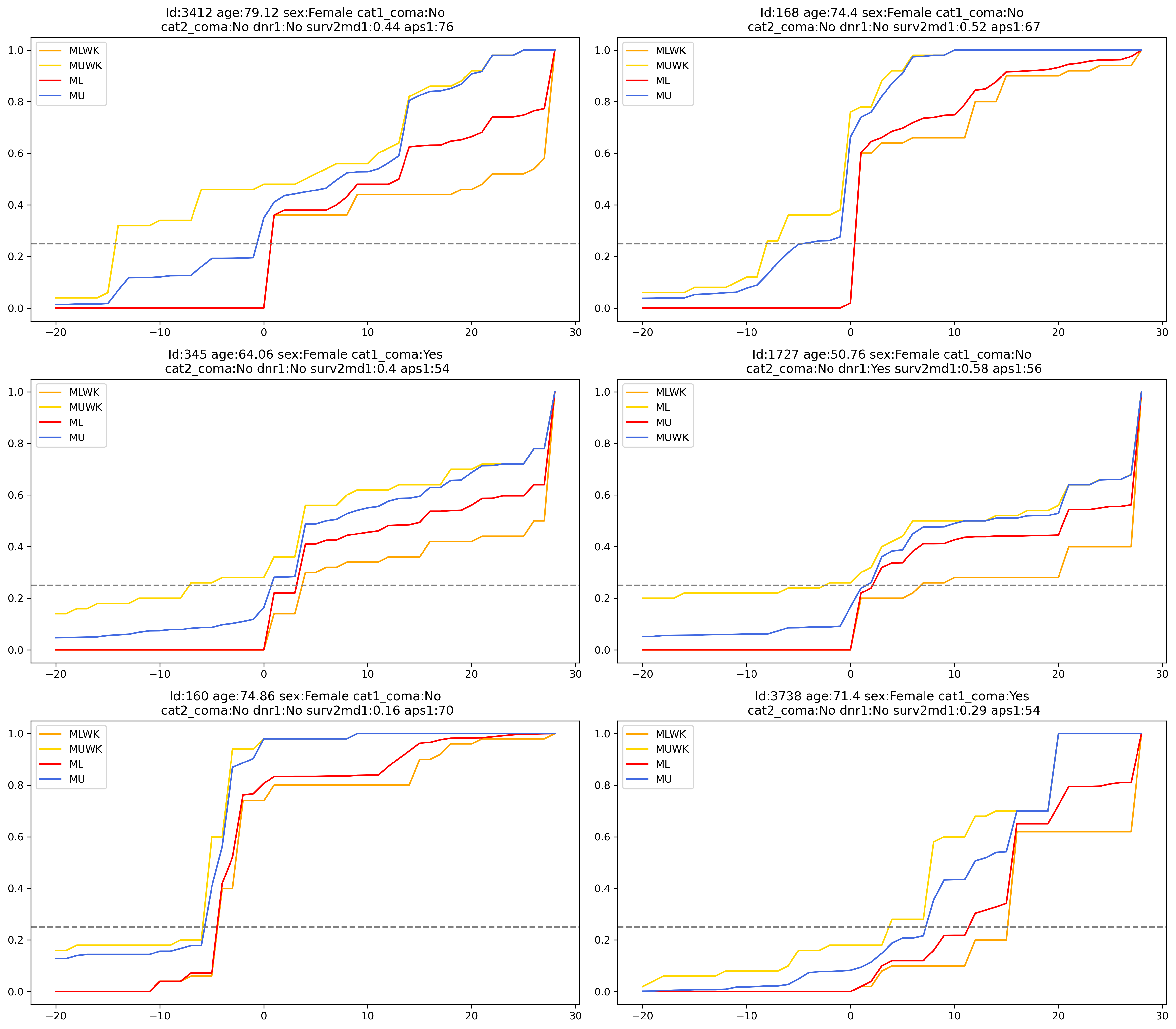
• In the figure, the vertical line indicates zero and the horizontal line indicates $\tau=0.25$.

Figure 1: Bounds on the QoTE of Six Representative Patients

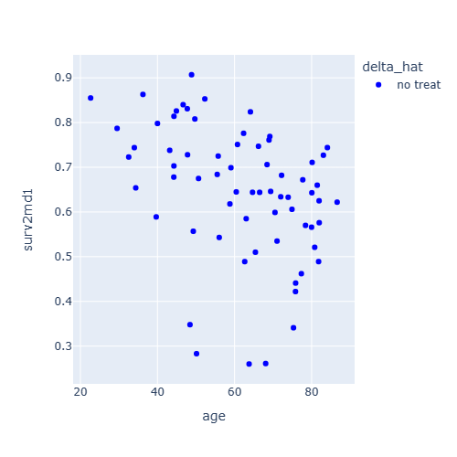
(a) QoTE with $\tau=0.25$

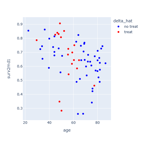
(b) QoTE with $\tau=0.5$

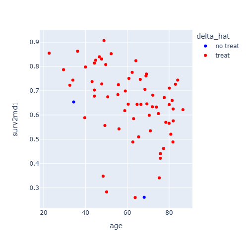
(c) QoTE with $\tau=0.75$

Figure 2: Treatment Decisions for Male Patients with Specific Health Conditions

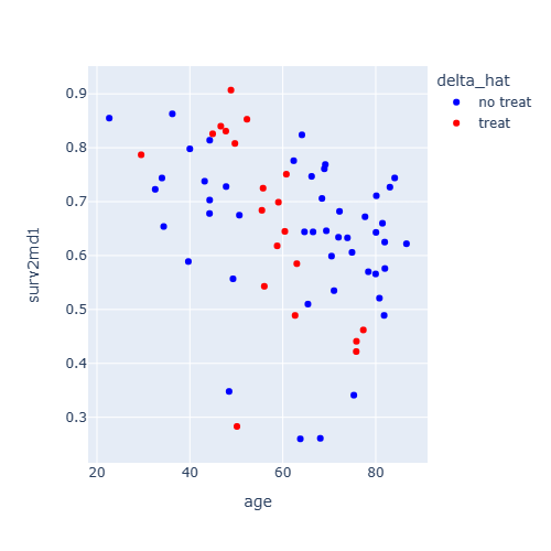
(a) QTE with $\tau=0.25$

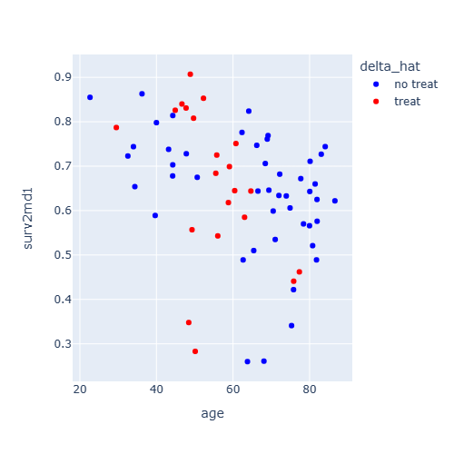
(b) QTE with $\tau=0.5$

(c) QTE with $\tau=0.75$

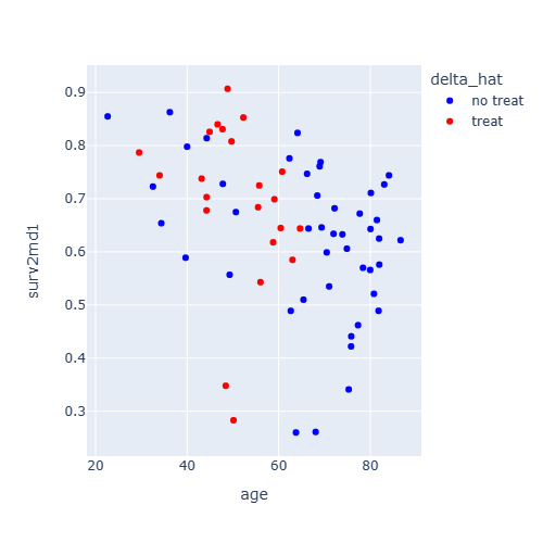
(d) ATE

Figure 3: Treatment Decisions Based on the QTEs and the ATE

6.2 Application II: Allocation of Job Training

The dataset is collected from the National Job Training Partnership Act (JTPA) Study (Bloom et al. (1997)). We use a subset that includes 9,223 adults; 6,133 of them received job training, while the remaining 3,090 did not. The treatment $D$ in question is the job training. In this experiment, we use the 30-month earnings after the job training program as the measure of outcome $Y$ and the sex, years of education, high school diploma, and previous earnings in $10K before the program as covariates $X$. Based on the data, the kernel regression has been conducted in the treatment and control groups separately to obtain the $\hat{F}_{Y_{1}|X}$ and $\hat{F}_{Y_{0}|X}$. From the estimated conditional distributions, we obtain the upper and lower bounds under SI (i.e., Assumption PD(iii)) and no assumption for each individual.

In Table 2 and Figure 4, we present six cases and their covariates to show bounds on the QoTE (i.e., the effect of job training on earnings) under SI and no assumption. Similar to the first application, we find heterogeneity in the treatment effects and thus the optimal decisions, but less so than the first application.

Next, in Figure 5, we present the decisions of allocating the job training to the female group without a high school diploma in the space of education and previous earnings (i.e., the two important covariates for the allocation decision). Again, we use the 0.25-quantile, median, and 0.75-quantile QoTE bounds to represent prudent, majority-minded, and negligent PMs, respectively. The 0.75-quantile bounds suggest the treatment option more often than the other cases. It would be compelling to treat workers suggested by the 0.25-quantile bounds, as they produce prudent decisions.

For comparison, in Figure 6, we present the decisions based on the 0.25-quantile, median, and 0.75-quantile QTE and the ATE. Again, there is no obvious tendency in decisions when the quantile probability increases from 0.25 to 0.75, which reflects the limitation of using the QTE as the basis for decisions (e.g., the quantile probability does not capture the level of prudence). The decisions based on the ATE (i.e., the most common approach in the literature) look very similar to the decisions based on the median QoTE bounds, which suggests that the issue of outliers is not serious in this application. In this sense, the policy based on the median QoTE bounds can be viewed as a robustness check for the policy based on the ATE (e.g., Kitagawa and Tetenov (2018)).

Worker ID	$(Q_{\tau}^{L},Q_{\tau}^{U})$	$\hat{\delta}$	$(Q_{\tau}^{L,SI},Q_{\tau}^{U,SI})$	$\hat{\delta}^{SI}$
317237	$(-14.27,0.69)$	$0$	$(-1.44,0.83)$	$0$
310493	$(-8.07,0.40)$	$0$	$(-0.37,0.45)$	$1$
302861	$(-7.17,3.69)$	$0$	$(0.13,0.44)$	$1$
302890	$(-2.50,6.75)$	$1$	$(-2.23,-0.02)$	$0$
305160	$(-5.88,-4.44)$	$0$	$(-3.09,-2.48)$	$0$
303890	$(3.7,15.12)$	$1$	$(-3.21,-1.19)$	$0$

Table 2: Bounds on the QoTE ($\tau=0.25$) and Estimated Policies

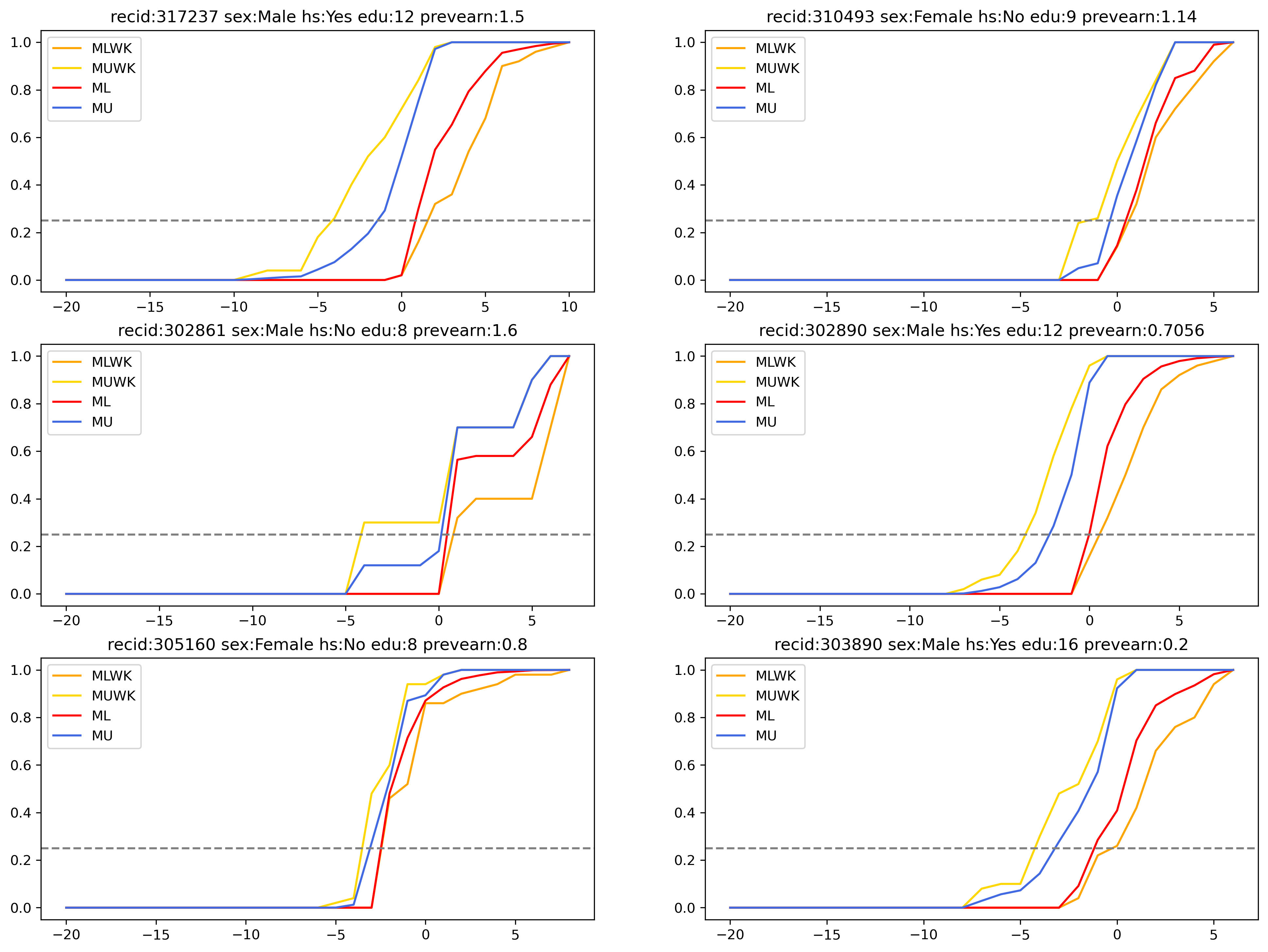
• In the figure, the vertical line indicates zero and the horizontal line indicates $\tau=0.25$.

Figure 4: Bounds on the QoTE of Six Representative Workers

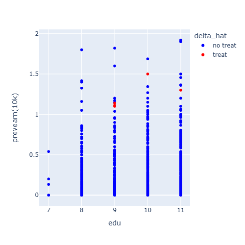
(a) QoTE with $\tau=0.25$

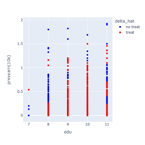
(b) QoTE with $\tau=0.5$

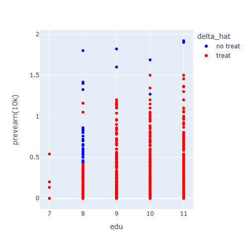
(c) QoTE with $\tau=0.75$

Figure 5: Treatment Decisions for Female Workers Without High School Diploma

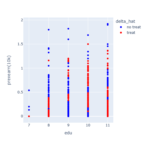
(a) QTE with $\tau=0.25$

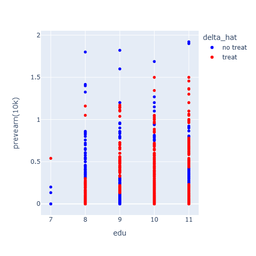
(b) QTE with $\tau=0.5$

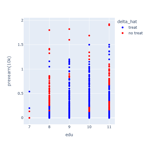
(c) QTE with $\tau=0.75$

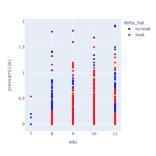
(d) ATE

Figure 6: Treatment Decisions Based on the QTEs and the ATE

7 Generalization

The joint distribution of the potential outcomes may contain other useful information about treatment effect heterogeneity for policy learning. The theoretical results of this paper can be generalized to any setting where welfare is defined as a functional of the joint distribution of potential outcomes. Consider an optimal rule that satisfies

$$\delta^{**} \in\arg\max_{\delta\in\mathcal{D}}E\left[\delta(X)\Lambda(F_{Y_{1},Y_{0}|X})\right],$$ (7.1)

where $\Lambda:\tilde{\mathcal{F}}\rightarrow\mathbb{R}$ is some functional of the joint distribution of $(Y_{1},Y_{0})$ given $X$. Our original criterion (2.2) is a special case of (7.1) with $\Lambda(F_{Y_{1},Y_{0}|X})=Q_{\tau}(Y_{1}-Y_{0}|X)$. We propose other examples of the criterion $\Lambda(F_{Y_{1},Y_{0}|X})$ that may interest a non-utilitarian PM.

Example 1.

Consider

$$\delta_{\bar{y}}^{**} \in\arg\max_{\delta\in\mathcal{D}}E\left[\delta(X)E[Y_{1}-Y_{0}|Y_{0}<\bar{y},X]\right]$$ (7.2)

for some predetermined $\bar{y}$. This can be motivated by maximizing the average of $\delta(X)Y_{1}+(1-\delta(X))Y_{0}$ (or simply $Y_{\delta(X)}$ with deterministic $\delta$), conditional on $Y_{0}<\bar{y}$:

$$\delta_{\bar{y}}^{**} \in\arg\max_{\delta\in\mathcal{D}}E\left[\delta(X)Y_{1}+(1-\delta(X))Y_{0}|Y_{0}<\bar{y}\right],$$ (7.3)

because $E[\delta(X)Y_{1}+(1-\delta(X))Y_{0}|Y_{0}<\bar{y}]=E[Y_{0}|Y_{0}<\bar{y}]+E[\delta(X)E[Y_{1}-Y_{0}|Y_{0}<\bar{y},X]]$. The PM with the criterion (7.3) focuses on the welfare of a disadvantaged population, defined by the baseline outcome $Y_{0}$ being less than $\bar{y}$. A similar intuition applies to the criterion (7.2), which can be interpreted as addressing the average gain for the disadvantaged. The ATE for the disadvantaged, $E[Y_{1}-Y_{0}|Y_{0}<\bar{y}]$, appears as a parameter of interest in the context of policy evaluation (Heckman and Smith (1995)), which is adapted here for the context of optimal allocation.

Example 2.

Alternative to Example 1, one can consider $\Lambda(F_{Y_{1},Y_{0}|X})=Q_{\tau}(Y_{1}-Y_{0}|Y_{0}<\bar{y},X)$. This would make the criterion robust to outliers and add an additional dimension, $\tau$, to target a specific subgroup. Analogous to Theorem 2.1, for continuously distributed $Y_{d}$ and deterministic policy $\delta$, the first-best policy under $Q_{0.5}(Y_{1}-Y_{0}|Y_{0}<\bar{y},X)$ is the one that maximizes $P\left[Y_{\delta(X)}-Y_{1-\delta(X)}>0|Y_{0}<\bar{y}\right]=P\left[\delta\in\arg\max_{d}Y_{d}|Y_{0}<\bar{y}\right]$.

Example 3.

One may wish to target individuals worst-affected by the treatment rather than those who are worst off at baseline. The conditional value at risk (CVaR) of the distribution of individual treatment effects can serve just that: $\Lambda(F_{Y_{1},Y_{0}|X})=E[Y_{1}-Y_{0}|Y_{1}-Y_{0}<\bar{\Delta},X]$. Kallus (2023) considers the CVaR, $E[Y_{1}-Y_{0}|Y_{1}-Y_{0}<\bar{\Delta}]$ with $\bar{\Delta}=Q_{\tau}(Y_{1}-Y_{0})$, as a parameter related to distributional treatment effects and provides a sharp upper bound and, under restricted heterogeneity, a sharp lower bound on the CVaR.

In all these examples, $\Lambda(F_{Y_{1},Y_{0}|X})$ is not generally point-identified, so one can follow the approach in Section 2.3 by considering

$$\delta_{mmr}^{**} \in\arg\min_{\delta\in\mathcal{D}}\max_{F_{Y_{1},Y_{0}|X}\in\mathcal{F}}E\left[\delta(X)\Lambda(F_{Y_{1},Y_{0}|X})\right].$$

Then, one can apply the identifying assumptions listed in Section 3 and the computational method proposed in Section 5 to systematically calculate the bounds on $\Lambda(F_{Y_{1},Y_{0}|X})$ and to eventually estimate $\delta_{mmr}^{**}$. Let $\Lambda^{L}(X)$ and $\Lambda^{U}(X)$ be the lower and upper bounds on $\Lambda(F_{Y_{1},Y_{0}|X})$. Then the theoretical properties of the estimated policies with constrained and unconstrained policy classes can be established based on Section 4 by simply replacing $Q_{\tau}^{L}(X)$ and $Q_{\tau}^{U}(X)$ with $\Lambda^{L}(X)$ and $\Lambda^{U}(X)$ throughout the section.

Appendix A Numerical Illustrations

The question we want to answer via numerical exercises is: how the performance of treatment allocations differ across welfare criteria, especially when the QoTE is partially identified. To facilitate illustration, we focus on in the case of unconstrained $\mathcal{D}$ and no $X$.

A.1 Simulation Design

We consider the following data-generating processes (DGPs). We draw either $(Y_{1},Y_{0})$ or $(\log Y_{1},\log Y_{0})$ from $N(\mu,\Sigma)$, where $\mu=(\mu_{1},\mu_{0})^{\prime}$ and $\Sigma=\bigl{(}\begin{smallmatrix}\sigma_{1}&\rho_{10}\sqrt{\sigma_{0}\sigma_{1}}\\ \rho_{10}\sqrt{\sigma_{0}\sigma_{1}}&\sigma_{0}\end{smallmatrix}\bigr{)}$, and $D$ independently from $Bernoulli(0.5)$. Then, the observed outcome is generated by $Y=DY_{1}+(1-D)Y_{0}$. Note that, under the bivariate normal distribution, $Y_{1}|Y_{0}\sim N(\mu_{1}+\rho_{10}\sigma_{1}Z_{0},(1-\rho^{2}\sigma_{1}))$ where $Z_{0}=\frac{Y_{0}-\mu_{0}}{\sigma_{0}}$. Therefore, $Y_{1}$ and $Y_{0}$ satisfying stochastically increasingness (SI) (i.e., Assumption PD(iii)) when $\rho_{10}\geq 0$. In fact, this is also true when $Y_{1}$ and $Y_{0}$ are bivariate log-normal; they are stochastically increasing when $\rho_{10}\geq 0$. When $\mathcal{D}$ is unrestricted, the true optimal policies based on the QoTE, QTE and ATE can be written as follows:

$$\delta^{*}=1\{Q_{\tau}(Y_{1}-Y_{0})>0\}\quad\text{where }Q_{\tau}(Y_{1}-Y_{0})=\mu_{1}-\mu_{0}+\Phi^{-1}(\tau)\sqrt{\sigma_{1}^{2}+\sigma_{0}^{2}-2\rho_{10}\sigma_{1}\sigma_{0}},$$

$$\delta_{QTE}^{*}=1\{Q_{\tau}(Y_{1})-Q_{\tau}(Y_{0})>0\}\quad\text{where }Q_{\tau}(Y_{1})-Q_{\tau}(Y_{0})=\mu_{1}-\mu_{0}+\Phi^{-1}(\tau)(\sigma_{1}-\sigma_{0}),$$

$$\delta_{ATE}^{*}=1\{E[Y_{1}-Y_{0}]>0\}\quad\text{where }E[Y_{1}-Y_{0}]=\mu_{1}-\mu_{0}.$$

Note that these policies are first-best regardless of whether we consider a deterministic or stochastic policy. Unlike $\delta_{QTE}^{*}$ and $\delta_{ATE}^{*}$, the proposed $\delta^{*}$ involves model uncertainty. Therefore we consider $\delta_{mmr}^{*}$ that minimizes (4.1). Its expression for the optimal deterministic and stochastic policies $\delta^{*,determ}$ and $\delta^{*,stoch}$ are given in Section 4.1.

In simulation, the bounds $Q_{\tau}^{L}$ and $Q_{\tau}^{U}$ are calculated under either no assumption (i.e., Makarov bounds) or SI. Under the latter, we use discretization to calculate the bounds. For the population policies $\delta_{mmr}^{*}$, $\delta_{QTE}^{*}$ and $\delta_{ATE}^{*}$, we estimate their sample counterparts $\hat{\delta}^{*}$, $\hat{\delta}_{QTE}^{*}$ and $\hat{\delta}_{ATE}^{*}$ by estimating $Q_{\tau}^{U}$, $Q_{\tau}^{L}$, $Q_{\tau}(Y_{d})$, and $E[Y_{d}]$ ($d=0,1$). Since $D$ is exogenous in our simulated data, $Q_{\tau}(Y_{d})=Q_{\tau}(Y|D=d)$ and $E[Y_{d}]=E[Y|D=d]$. For each estimate $\hat{\delta}_{j}$ of $\delta_{j}^{*}$ ($j\in\{\emptyset,QTE,ATE\}$), the misclassification error is $\mathbb{E}_{n}[1\{\hat{\delta}_{j}\neq\delta_{j}^{*}\}]$ and regret is defined as $\mathbb{E}_{n}[|T_{j}|\cdot 1\{\hat{\delta}_{j}\neq\delta_{j}^{*}\}]$ where $T=Q_{\tau}(Y_{1}-Y_{0})$, $T_{QTE}=Q_{\tau}(Y_{1})-Q_{\tau}(Y_{0})$, and $T_{ATE}=E[Y_{1}-Y_{0}]$ are the corresponding treatment effects (or equivalently the welfare gains). We focus on $\tau=0.25$.

A.2 Simulation Results

Tables 3–4 present the simulated correct classification rates of the estimated policies relative to the (true) population policies. We set $n=1000$ for Table 3 and $n=50$ for Table 4. To calculate each classification rate, we replicate each experiment $200$ times. We consider both the correct specification of SI and misspecification. We also vary the parameter values in the normal and log-normal distributions. We treat each DGP as a subgroup of population (as if it corresponds to a particular value of $X$ if covariates were to be introduced). Subgroups 1–4 and 7 follow the normal distribution and SI, and Subgroups 5–6 are where SI is violated. Under bivariate normality and SI, if $0<\tau<0.5$, $Q_{\tau}(Y_{1}-Y_{0})<Q_{\tau}(Y_{1})-Q_{\tau}(Y_{0})$ and $Q_{\tau}(Y_{1}-Y_{0})<E(Y_{1})-E(Y_{0})$. The purpose of Subgroup 8 is to break this mechanical relationship. Subgroup 8 follows the log-normal distribution and SI.

	$\hat{\delta}^{stoch,SI}$	$\hat{\delta}^{stoch}$	$\hat{\delta}^{determ,SI}$	$\hat{\delta}^{determ}$	$\hat{\delta}_{QTE}$	$\hat{\delta}_{ATE}$
	Subgroup 1
$\delta^{*}$	$100\%$	$100\%$	$100\%$	$100\%$	$1.5\%$	$100\%$
$\delta_{QTE}^{*}$	$0\%$	$0\%$	$0\%$	$0\%$	$98.5\%$	$0\%$
$\delta_{ATE}^{*}$	$100\%$	$100\%$	$100\%$	$100\%$	$1.5\%$	$100\%$
	Subgroup 2
$\delta^{*}$	$100\%$	$99\%$	$100\%$	$100\%$	$0\%$	$0\%$
$\delta_{QTE}^{*}$	$0\%$	$1\%$	$0\%$	$0\%$	$100\%$	$100\%$
$\delta_{ATE}^{*}$	$0\%$	$1\%$	$0\%$	$0\%$	$100\%$	$100\%$
	Subgroup 3
$\delta^{*}$	$89\%$	$59\%$	$100\%$	$95\%$	$100\%$	$100\%$
$\delta_{QTE}^{*}$	$89\%$	$59\%$	$100\%$	$95\%$	$100\%$	$100\%$
$\delta_{ATE}^{*}$	$89\%$	$59\%$	$100\%$	$95\%$	$100\%$	$100\%$
	Subgroup 4
$\delta^{*}$	$21\%$	$43\%$	$0\%$	$20\%$	$0\%$	$0\%$
$\delta_{QTE}^{*}$	$79\%$	$57\%$	$100\%$	$80\%$	$100\%$	$100\%$
$\delta_{ATE}^{*}$	$79\%$	$57\%$	$100\%$	$80\%$	$100\%$	$100\%$
	Subgroup 5
$\delta^{*}$	$92\%$	$74\%$	$100\%$	$100\%$	$100\%$	$0\%$
$\delta_{QTE}^{*}$	$92\%$	$74\%$	$100\%$	$100\%$	$100\%$	$0\%$
$\delta_{ATE}^{*}$	$8\%$	$26\%$	$0\%$	$0\%$	$0\%$	$100\%$
	Subgroup 6
$\delta^{*}$	$34\%$	$48\%$	$6.5\%$	$86\%$	$0\%$	$0\%$
$\delta_{QTE}^{*}$	$66\%$	$52\%$	$93.5\%$	$14\%$	$100\%$	$100\%$
$\delta_{ATE}^{*}$	$66\%$	$52\%$	$93.5\%$	$14\%$	$100\%$	$100\%$
	Subgroup 7
$\delta^{*}$	$76.5\%$	$53\%$	$100\%$	$31.5\%$	$100\%$	$100\%$
$\delta_{QTE}^{*}$	$76.5\%$	$53\%$	$100\%$	$31.5\%$	$100\%$	$100\%$
$\delta_{ATE}^{*}$	$76.5\%$	$53\%$	$100\%$	$31.5\%$	$100\%$	$100\%$
	Subgroup 8 (log normal)
$\delta^{*}$	$99.5\%$	$48\%$	$100\%$	$32.5\%$	$100\%$	$4.5\%$
$\delta_{QTE}^{*}$	$99.5\%$	$48\%$	$100\%$	$32.5\%$	$100\%$	$4.5\%$
$\delta_{ATE}^{*}$	$0\%$	$52\%$	$0\%$	$67.5\%$	$0\%$	$95.5\%$

Table 3: Correct Classification Rate ($\tau=0.25$, $n=1000$)

	$\hat{\delta}^{stoch,SI}$	$\hat{\delta}^{stoch}$	$\hat{\delta}^{determ,SI}$	$\hat{\delta}^{determ}$	$\hat{\delta}_{QTE}$	$\hat{\delta}_{ATE}$
	Subgroup 1
$\delta^{*}$	$100\%$	$100\%$	$100\%$	$100\%$	$33.5\%$	$93\%$
$\delta_{QTE}^{*}$	$0\%$	$0\%$	$0\%$	$0\%$	$66.5\%$	$7\%$
$\delta_{ATE}^{*}$	$100\%$	$100\%$	$100\%$	$100\%$	$33.5\%$	$93\%$
	Subgroup 2
$\delta^{*}$	$92\%$	$90\%$	$90.5\%$	$94\%$	$1\%$	$17\%$
$\delta_{QTE}^{*}$	$8\%$	$10\%$	$9.5\%$	$6\%$	$99\%$	$83\%$
$\delta_{ATE}^{*}$	$8\%$	$10\%$	$9.5\%$	$6\%$	$99\%$	$83\%$
	Subgroup 3
$\delta^{*}$	$79\%$	$51\%$	$84\%$	$62\%$	$99.5\%$	$100\%$
$\delta_{QTE}^{*}$	$79\%$	$51\%$	$84\%$	$62\%$	$99.5\%$	$100\%$
$\delta_{ATE}^{*}$	$79\%$	$51\%$	$84\%$	$62\%$	$99.5\%$	$100\%$
	Subgroup 4
$\delta^{*}$	$26\%$	$49.5\%$	$14.5\%$	$44\%$	$1.5\%$	$0.5\%$
$\delta_{QTE}^{*}$	$74\%$	$50.5\%$	$85.5\%$	$56\%$	$98.5\%$	$99.5\%$
$\delta_{ATE}^{*}$	$74\%$	$50.5\%$	$85.5\%$	$56\%$	$98.5\%$	$99.5\%$
	Subgroup 5
$\delta^{*}$	$82\%$	$81\%$	$83\%$	$93.5\%$	$66.5\%$	$4\%$
$\delta_{QTE}^{*}$	$82\%$	$81\%$	$83\%$	$93.5\%$	$66.5\%$	$4\%$
$\delta_{ATE}^{*}$	$18\%$	$19\%$	$17\%$	$6.5\%$	$33.5\%$	$96\%$
	Subgroup 6
$\delta^{*}$	$43\%$	$61.5\%$	$40\%$	$61\%$	$24\%$	$0\%$
$\delta_{QTE}^{*}$	$57\%$	$38.5\%$	$60\%$	$39\%$	$76\%$	$100\%$
$\delta_{ATE}^{*}$	$57\%$	$38.5\%$	$60\%$	$39\%$	$76\%$	$100\%$
	Subgroup 7
$\delta^{*}$	$71.5\%$	$48\%$	$80\%$	$49.5\%$	$96\%$	$99.5\%$
$\delta_{QTE}^{*}$	$71.5\%$	$48\%$	$80\%$	$49.5\%$	$96\%$	$99.5\%$
$\delta_{ATE}^{*}$	$71.5\%$	$48\%$	$80\%$	$49.5\%$	$96\%$	$99.5\%$
	Subgroup 8 (log normal)
$\delta^{*}$	$81\%$	$53\%$	$85\%$	$48\%$	$100\%$	$58.5\%$
$\delta_{QTE}^{*}$	$81\%$	$53\%$	$85\%$	$48\%$	$100\%$	$58.5\%$
$\delta_{ATE}^{*}$	$19\%$	$47\%$	$15\%$	$52\%$	$0\%$	$41.5\%$

Table 4: Correct Classification Rate ($\tau=0.25$, $n=50$)

Here are the summary of the features in the DGP and corresponding results in Tables 3–4. Recall that $\tau=0.25$.

Overall, the correct classification rate tends to be high when the welfare criterion of the estimated policy matches that of the population policy.

Subgroup 1: Both intervals under SI and no assumption exclude $0$ and lie relatively far from it; therefore, both $\hat{\delta}$ and $\hat{\delta}^{SI}$ perform well; $\delta_{QTE}^{*}\neq\delta^{*}=\delta_{ATE}^{*}$.

Subgroup 2: Both intervals under SI and no assumption exclude 0; $\hat{\delta}^{determ}$ does not perform worse than $\hat{\delta}^{determ,SI}$ for $\delta^{*}$ because $Q_{\tau}^{L,SI}-Q_{\tau}^{L}>Q_{\tau}^{U}-Q_{\tau}^{U,SI}$; $\delta^{*}\neq\delta_{QTE}^{*}=\delta_{ATE}^{*}$.

Subgroup 3: Both intervals under SI and no assumption cover 0 (and the same holds for Subgroups 4–7); $\hat{\delta}^{SI}$ performs better than $\hat{\delta}$; $Q_{\tau}^{L,SI}-Q_{\tau}^{L}>Q_{\tau}^{U}-Q_{\tau}^{U,SI}$ and, under the bivariate normal distribution and SI, $Q_{\tau}(Y_{1}-Y_{0})<Q_{\tau}(Y_{1})-Q_{\tau}(Y_{0})$ and $Q_{\tau}(Y_{1}-Y_{0})<E(Y_{1})-E(Y_{0})$ always hold, and thus both $\hat{\delta}_{QTE}$ and $\hat{\delta}_{ATE}$ perform well; $\delta^{*}=\delta_{QTE}^{*}=\delta_{ATE}^{*}=1$.

Subgroup 4: Both $\hat{\delta}^{SI}$ and $\hat{\delta}$ perform poorly for $\delta^{*}$ because the bound on $Q_{\tau}(Y_{1}-Y_{0})$ covers zero, and the difference between the upper bound and zero is larger than the difference between the lower bound and zero; $\delta^{*}\neq\delta_{QTE}^{*}=\delta_{ATE}^{*}$.

Subgroup 5: SI is false but $\hat{\delta}^{SI}$ does not perform so poorly because $Q_{\tau}(Y_{1}-Y_{0})$ is still covered by a relatively long interval; for the same reason, $\hat{\delta}$ does not perform significantly better; $\delta^{*}=\delta_{QTE}^{*}\neq\delta_{ATE}^{*}$.

Subgroup 6: SI is false and $\hat{\delta}^{SI}$ performs poorly because $Q_{\tau}(Y_{1}-Y_{0})$ is not covered by a relatively long interval; $\hat{\delta}$ does not perform well because $Q_{\tau}^{L,SI}-Q_{\tau}^{L}<Q_{\tau}^{U}-Q_{\tau}^{U,SI}$; $\delta^{*}\neq\delta_{QTE}^{*}=\delta_{ATE}^{*}$.

Subgroup 7: $\hat{\delta}^{SI}$ makes a correct decision while $\hat{\delta}$ performs worse; meanwhile, $\hat{\delta}_{QTE}$ and $\hat{\delta}_{ATE}$ perform well.

Subgroup 8: The interval under SI excludes $0$ while the interval under no assumption covers $0$; therefore, $\hat{\delta}^{SI}$ performs better than $\hat{\delta}$; under this log-normal setting and SI, $Q_{\tau}(Y_{1}-Y_{0})<E(Y_{1})-E(Y_{0})$ may be violated, which occurs in the current subgroup and thus $\hat{\delta}^{SI}$ performs better than $\hat{\delta}_{ATE}$.

A.3 Additional Simulation Results

Tables 5 and 6 present the classification rates with $\tau=0.75$.

	$\hat{\delta}^{stoch,SI}$	$\hat{\delta}^{stoch}$	$\hat{\delta}^{determ,SI}$	$\hat{\delta}^{determ}$	$\hat{\delta}_{QTE}$	$\hat{\delta}_{ATE}$
	Subgroup 1
$\delta^{*}$	$100\%$	$100\%$	$100\%$	$100\%$	$1.5\%$	$100\%$
$\delta_{QTE}^{*}$	$0\%$	$0\%$	$0\%$	$0\%$	$98.5\%$	$0\%$
$\delta_{ATE}^{*}$	$100\%$	$100\%$	$100\%$	$100\%$	$1.5\%$	$100\%$
	Subgroup 2
$\delta^{*}$	$100\%$	$99\%$	$100\%$	$100\%$	$0\%$	$0\%$
$\delta_{QTE}^{*}$	$0\%$	$1\%$	$0\%$	$0\%$	$100\%$	$100\%$
$\delta_{ATE}^{*}$	$0\%$	$1\%$	$0\%$	$0\%$	$100\%$	$100\%$
	Subgroup 3
$\delta^{*}$	$89\%$	$59\%$	$100\%$	$95\%$	$100\%$	$100\%$
$\delta_{QTE}^{*}$	$89\%$	$59\%$	$100\%$	$95\%$	$100\%$	$100\%$
$\delta_{ATE}^{*}$	$89\%$	$59\%$	$100\%$	$95\%$	$100\%$	$100\%$
	Subgroup 4
$\delta^{*}$	$21\%$	$43\%$	$0\%$	$20\%$	$0\%$	$0\%$
$\delta_{QTE}^{*}$	$79\%$	$57\%$	$100\%$	$80\%$	$100\%$	$100\%$
$\delta_{ATE}^{*}$	$79\%$	$57\%$	$100\%$	$80\%$	$100\%$	$100\%$
	Subgroup 5
$\delta^{*}$	$92\%$	$74\%$	$100\%$	$100\%$	$100\%$	$0\%$
$\delta_{QTE}^{*}$	$92\%$	$74\%$	$100\%$	$100\%$	$100\%$	$0\%$
$\delta_{ATE}^{*}$	$8\%$	$26\%$	$0\%$	$0\%$	$0\%$	$100\%$
	Subgroup 6
$\delta^{*}$	$34\%$	$48\%$	$6.5\%$	$86\%$	$0\%$	$0\%$
$\delta_{QTE}^{*}$	$66\%$	$52\%$	$93.5\%$	$14\%$	$100\%$	$100\%$
$\delta_{ATE}^{*}$	$66\%$	$52\%$	$93.5\%$	$14\%$	$100\%$	$100\%$
	Subgroup 7
$\delta^{*}$	$76.5\%$	$53\%$	$100\%$	$31.5\%$	$100\%$	$100\%$
$\delta_{QTE}^{*}$	$76.5\%$	$53\%$	$100\%$	$31.5\%$	$100\%$	$100\%$
$\delta_{ATE}^{*}$	$76.5\%$	$53\%$	$100\%$	$31.5\%$	$100\%$	$100\%$
	Subgroup 8 (log normal)
$\delta^{*}$	$99.5\%$	$48\%$	$100\%$	$32.5\%$	$100\%$	$4.5\%$
$\delta_{QTE}^{*}$	$99.5\%$	$48\%$	$100\%$	$32.5\%$	$100\%$	$4.5\%$
$\delta_{ATE}^{*}$	$0\%$	$52\%$	$0\%$	$67.5\%$	$0\%$	$95.5\%$

Table 5: Correct Classification Rate ($\tau=0.75$, $n=1000$)

	$\hat{\delta}^{stoch,SI}$	$\hat{\delta}^{stoch}$	$\hat{\delta}^{determ,SI}$	$\hat{\delta}^{determ}$	$\hat{\delta}_{QTE}$	$\hat{\delta}_{ATE}$
	Subgroup 1
$\delta^{*}$	$100\%$	$100\%$	$100\%$	$100\%$	$33.5\%$	$93\%$
$\delta_{QTE}^{*}$	$0\%$	$0\%$	$0\%$	$0\%$	$66.5\%$	$7\%$
$\delta_{ATE}^{*}$	$100\%$	$100\%$	$100\%$	$100\%$	$33.5\%$	$93\%$
	Subgroup 2
$\delta^{*}$	$92\%$	$90\%$	$90.5\%$	$94\%$	$1\%$	$17\%$
$\delta_{QTE}^{*}$	$8\%$	$10\%$	$9.5\%$	$6\%$	$99\%$	$83\%$
$\delta_{ATE}^{*}$	$8\%$	$10\%$	$9.5\%$	$6\%$	$99\%$	$83\%$
	Subgroup 3
$\delta^{*}$	$79\%$	$51\%$	$84\%$	$62\%$	$99.5\%$	$100\%$
$\delta_{QTE}^{*}$	$79\%$	$51\%$	$84\%$	$62\%$	$99.5\%$	$100\%$
$\delta_{ATE}^{*}$	$79\%$	$51\%$	$84\%$	$62\%$	$99.5\%$	$100\%$
	Subgroup 4
$\delta^{*}$	$26\%$	$49.5\%$	$14.5\%$	$44\%$	$1.5\%$	$0.5\%$
$\delta_{QTE}^{*}$	$74\%$	$50.5\%$	$85.5\%$	$56\%$	$98.5\%$	$99.5\%$
$\delta_{ATE}^{*}$	$74\%$	$50.5\%$	$85.5\%$	$56\%$	$98.5\%$	$99.5\%$
	Subgroup 5
$\delta^{*}$	$82\%$	$81\%$	$83\%$	$93.5\%$	$66.5\%$	$4\%$
$\delta_{QTE}^{*}$	$82\%$	$81\%$	$83\%$	$93.5\%$	$66.5\%$	$4\%$
$\delta_{ATE}^{*}$	$18\%$	$19\%$	$17\%$	$6.5\%$	$33.5\%$	$96\%$
	Subgroup 6
$\delta^{*}$	$43\%$	$61.5\%$	$40\%$	$61\%$	$24\%$	$0\%$
$\delta_{QTE}^{*}$	$57\%$	$38.5\%$	$60\%$	$39\%$	$76\%$	$100\%$
$\delta_{ATE}^{*}$	$57\%$	$38.5\%$	$60\%$	$39\%$	$76\%$	$100\%$
	Subgroup 7
$\delta^{*}$	$71.5\%$	$48\%$	$80\%$	$49.5\%$	$96\%$	$99.5\%$
$\delta_{QTE}^{*}$	$71.5\%$	$48\%$	$80\%$	$49.5\%$	$96\%$	$99.5\%$
$\delta_{ATE}^{*}$	$71.5\%$	$48\%$	$80\%$	$49.5\%$	$96\%$	$99.5\%$
	Subgroup 8 (log normal)
$\delta^{*}$	$81\%$	$53\%$	$85\%$	$48\%$	$100\%$	$58.5\%$
$\delta_{QTE}^{*}$	$81\%$	$53\%$	$85\%$	$48\%$	$100\%$	$58.5\%$
$\delta_{ATE}^{*}$	$19\%$	$47\%$	$15\%$	$52\%$	$0\%$	$41.5\%$

Table 6: Correct Classification Rate ($\tau=0.75$, $n=50$)

The overall patterns are analogous to the case with $\tau=0.25$.

A.4 Details of the DGPs of Subgroups in Simulation

Tables 7 and 8 show the details of the DGPs and related outputs used in the simulation results of Sections A.2 (with $\tau=0.25$) and A.3 (with $\tau=0.75$), respectively.

Subgroup	$(\mu_{1},\mu_{0})$	$(\sigma_{1}^{2},\sigma_{0}^{2})$	$\rho_{10}$	$\delta^{*}$	$\delta_{QTE}^{*}$	$\delta_{ATE}^{*}$
1	$(2,3)$	$(1,9)$	$0.5$	$\begin{array}[]{c}0\\ (-2.97)\end{array}$	$\begin{array}[]{c}1\\ (0.34)\end{array}$	$\begin{array}[]{c}0\\ (-1)\end{array}$
2	$(4,3)$	$(1,25)$	$0.5$	$\begin{array}[]{c}0\\ (-2.09)\end{array}$	$\begin{array}[]{c}1\\ (3.7)\end{array}$	$\begin{array}[]{c}1\\ (1)\end{array}$
3	$(7,3)$	$(9,25)$	$0.5$	$\begin{array}[]{c}1\\ (1.1)\end{array}$	$\begin{array}[]{c}1\\ (5.35)\end{array}$	$\begin{array}[]{c}1\\ (4)\end{array}$
4	$(3,1)$	$(5,5)$	$0.1$	$\begin{array}[]{c}0\\ (-0.23)\end{array}$	$\begin{array}[]{c}1\\ (2)\end{array}$	$\begin{array}[]{c}1\\ (2)\end{array}$
5	$(3,2)$	$(9,1)$	$-0.5$	$\begin{array}[]{c}0\\ (-1.43)\end{array}$	$\begin{array}[]{c}0\\ (-0.35)\end{array}$	$\begin{array}[]{c}1\\ (1)\end{array}$
6	$(3,0)$	$(25,4)$	$-0.5$	$\begin{array}[]{c}0\\ (-1.21)\end{array}$	$\begin{array}[]{c}1\\ (0.98)\end{array}$	$\begin{array}[]{c}1\\ (3)\end{array}$
7	$(2,0)$	$(8,4)$	$0.5$	$\begin{array}[]{c}1\\ (0.30)\end{array}$	$\begin{array}[]{c}1\\ (1.44)\end{array}$	$\begin{array}[]{c}1\\ (2)\end{array}$
8	$(3,0)$	$(2,8)$	$0.8$	$\begin{array}[]{c}1\\ (\text{-})\end{array}$	$\begin{array}[]{c}1\\ (4.28)\end{array}$	$\begin{array}[]{c}0\\ (-1.5)\end{array}$

Subgroup	$Q_{\tau}^{L,SI}$	$Q_{\tau}^{U,SI}$	$Q_{\tau}^{L}$	$Q_{\tau}^{U}$	$\delta^{*,stoch,SI}$	$\delta^{*,stoch}$	$Y_{1}-Y_{0}$
1	$-3.48$	$-1.84$	$-5.1$	$-1.1$	$100\%$	$100\%$	$N(-1,7)$
2	$-2.8$	$-1.19$	$-4.50$	$-0.17$	$100\%$	$100\%$	$N(1,21)$
3	$-0.74$	$3.91$	$-4.83$	$5.63$	$84\%$	$54\%$	$N(4,19)$
4	$-0.68$	$2.54$	$-3.1$	$3.38$	$21\%$	$48\%$	$N(2,9)$
5	$-1.48$	$0.16$	$-3.1$	$0.9$	$90\%$	$77\%$	$N(1,13)$
6	$-1.24$	$1.92$	$-4.3$	$3.5$	$39\%$	$55\%$	$N(3,39)$
7	$-0.86$	$2.17$	$-3.37$	$3.21$	$72\%$	$49\%$	$N(2,12-4\sqrt{2})$
8	$0.38$	$6.57$	$-8.5$	$7.75$	$100\%$	$48\%$	-

• Subgroup 8 is under log-normal transformation, i.e., $(\log Y_{1},\log Y_{0})\sim N(\mu,\Sigma)$.

• In the parentheses of $\delta^{*}$, $\delta^{*}_{QTE}$, and $\delta^{*}_{ATE}$ are the values of $Q_{\tau}(Y_{1}-Y_{0})$, $Q_{\tau}(Y_{1})-Q_{\tau}(Y_{0})$, and $E[Y_{1}-Y_{0}]$, respectively.

Table 7: DGP and Population Values

Subgroup	$(\mu_{1},\mu_{0})$	$(\sigma_{1}^{2},\sigma_{0}^{2})$	$\rho_{10}$	$\delta^{*}$	$\delta_{QTE}^{*}$	$\delta_{ATE}^{*}$
1	$(2,3)$	$(1,9)$	$0.5$	$\begin{array}[]{c}1\\ (0.79)\end{array}$	$\begin{array}[]{c}0\\ (-2.35)\end{array}$	$\begin{array}[]{c}0\\ (-1)\end{array}$
2	$(4,3)$	$(1,25)$	$0.5$	$\begin{array}[]{c}1\\ (4.09)\end{array}$	$\begin{array}[]{c}0\\ (-1.70)\end{array}$	$\begin{array}[]{c}1\\ (1)\end{array}$
3	$(7,3)$	$(9,25)$	$0.5$	$\begin{array}[]{c}1\\ (6.94)\end{array}$	$\begin{array}[]{c}1\\ (2.65)\end{array}$	$\begin{array}[]{c}1\\ (4)\end{array}$
4	$(3,1)$	$(5,5)$	$0.1$	$\begin{array}[]{c}1\\ (4.02)\end{array}$	$\begin{array}[]{c}1\\ (2)\end{array}$	$\begin{array}[]{c}1\\ (2)\end{array}$
5	$(3,2)$	$(9,1)$	$-0.5$	$\begin{array}[]{c}1\\ (3.43)\end{array}$	$\begin{array}[]{c}1\\ (2.35)\end{array}$	$\begin{array}[]{c}1\\ (1)\end{array}$
6	$(3,0)$	$(25,4)$	$-0.5$	$\begin{array}[]{c}1\\ (7.21)\end{array}$	$\begin{array}[]{c}1\\ (5.02)\end{array}$	$\begin{array}[]{c}1\\ (3)\end{array}$
7	$(2,0)$	$(8,4)$	$0.5$	$\begin{array}[]{c}1\\ (3.70)\end{array}$	$\begin{array}[]{c}1\\ (2.56)\end{array}$	$\begin{array}[]{c}1\\ (2)\end{array}$
8	$(3,0)$	$(2,11)$	$0.8$	$\begin{array}[]{c}1\\ (\text{-})\end{array}$	$\begin{array}[]{c}1\\ (1.72)\end{array}$	$\begin{array}[]{c}0\\ (-1.5)\end{array}$

Subgroup	$Q_{\tau}^{L,SI}$	$Q_{\tau}^{U,SI}$	$Q_{\tau}^{L}$	$Q_{\tau}^{U}$	$\delta^{*,stoch,SI}$	$\delta^{*,stoch}$	$Y_{1}-Y_{0}$
1	$-0.16$	$1.48$	$-0.92$	$3.10$	$95\%$	$77\%$	$N(-1,7)$
2	$3.19$	$4.80$	$2.17$	$6.50$	$100\%$	$100\%$	$N(1,21)$
3	$4.08$	$8.74$	$2.37$	$12.83$	$100\%$	$100\%$	$N(4,19)$
4	$1.46$	$4.68$	$0.61$	$7.10$	$100\%$	$100\%$	$N(2,9)$
5	$1.84$	$3.48$	$1.08$	$5.10$	$100\%$	$100\%$	$N(1,13)$
6	$4.08$	$7.2$5	$2.50$	$10.25$	$100\%$	$100\%$	$N(3,39)$
7	$1.82$	$4.87$	$0.79$	$7.37$	$100\%$	$100\%$	$N(2,12-4\sqrt{2})$
8	$18.07$	$27.33$	$11.50$	$26.69$	$100\%$	$100\%$	-

• Subgroup 8 is under log-normal transformation, i.e., $(\log Y_{1},\log Y_{0})\sim N(\mu,\Sigma)$.

• In the parentheses of $\delta^{*}$, $\delta^{*}_{QTE}$, and $\delta^{*}_{ATE}$ are the values of $Q_{\tau}(Y_{1}-Y_{0})$, $Q_{\tau}(Y_{1})-Q_{\tau}(Y_{0})$, and $E[Y_{1}-Y_{0}]$, respectively.

Table 8: DGP and Population Values

Appendix B Welfare Criteria with Stochastic Rules

We present a more rigorous formulation of the welfare criteria in Section 2 when a stochastic rule is considered. Let $A(x)$ is a r.v. representing the stochastic rule drawn from Bernoulli with parameter $\delta(x)\equiv\Pr[A(x)=1|X=x]$. Then, by assuming $A(X)\perp Y_{d}|X$ for any $d$ (and using it in the third equality below), we have

$$E[A(X)Y_{1}+(1-A(X))Y_{0}] =E[Y_{0}]+E[A(X)(Y_{1}-Y_{0})]$$

$$=E[Y_{0}]+E[A(X)E[Y_{1}-Y_{0}|A(X),X]]$$

$$=E[Y_{0}]+E[A(X)E[Y_{1}-Y_{0}|X]]$$

$$=E[Y_{0}]+E[E[A(X)E[Y_{1}-Y_{0}|X]|X]]$$

$$=E[Y_{0}]+E[E[Y_{1}-Y_{0}|X]E[A(X)|X]]$$

$$=E[Y_{0}]+E[E[Y_{1}-Y_{0}|X]\delta(X)]$$

$$=E[\delta(X)Y_{1}+(1-\delta(X))Y_{0}].$$

Similarly, motivated from the third line above

$$E[A(X)Q(Y_{1}-Y_{0}|X)] =E[E[A(X)Q(Y_{1}-Y_{0}|X)|X]]$$

$$E[Q(Y_{1}-Y_{0}|X)E[A(X)|X]]$$

$$=E[Q(Y_{1}-Y_{0}|X)\delta(X)].$$

Based on these results, it suffices to use $\delta(x)$ for both deterministic and stochastic rules in Sections 4 and 7.

Appendix C Proofs

C.1 Proof of Lemma 4.1

Proof.

Fix $x$ and let $\bar{R}(\delta;x)\equiv\max_{Q_{\tau}(x)\in[Q_{\tau}^{L}(x),Q_{\tau}^{U}(x)]}|Q_{\tau}(x)|1\{A(x)\neq sign(Q_{\tau}(x))\}$. If $0\leq Q_{\tau}^{L}(x)\leq Q_{\tau}^{U}(x)$,

$$\bar{R}(\delta;x) =|Q_{\tau}^{U}(x)|1\{A(x)\neq 1\}=Q_{\tau}^{U}(x)1\{A(x)\neq 1\}$$

and if $0\geq Q_{\tau}^{U}(x)\geq Q_{\tau}^{L}(x)$,

$$\bar{R}(\delta;x) =|Q_{\tau}^{L}(x)|1\{A(x)\neq 0\}=-Q_{\tau}^{L}(x)1\{A(x)\neq 0\}.$$

Finally, if $Q_{\tau}^{L}(x)<0<Q_{\tau}^{U}(x)$,

$$\bar{R}(\delta;x) =|Q_{\tau}^{U}(x)|1\{A(x)\neq 1\}+|Q_{\tau}^{L}(x)|1\{A(x)\neq 0\}$$

$$=Q_{\tau}^{U}(x)1\{A(x)\neq 1\}-Q_{\tau}^{L}(x)1\{A(x)\neq 0\}.$$

Therefore, by the law of iterated expectation and Assumption RC, we have

$$\bar{R}(\delta) =E\left[Q_{\tau}^{U}(X)[1-\delta(X)]1\{Q_{\tau}^{L}(X)\geq 0\}-Q_{\tau}^{L}(X)\delta(X)1\{Q_{\tau}^{U}(X)\leq 0\}\right.$$

$$+Q_{\tau}^{U}(X)[1-\delta(X)]1\{Q_{\tau}^{L}(X)<0<Q_{\tau}^{U}(X)\}-Q_{\tau}^{L}(X)\delta(X)1\{Q_{\tau}^{L}(X)<0<Q_{\tau}^{U}(X)\}\bigg{]}.$$ (C.1)

From (C.1), it is straightforward to show (4.2) and (4.3). To show (4.4), note that, if $Q_{\tau}^{L}(x)<0<Q_{\tau}^{U}(x)$,

$$Q_{\tau}^{U}(x)1\{A(x)\neq 1\}-Q_{\tau}^{L}(x)1\{A(x)\neq 0\}$$

$$=|Q_{\tau}^{U}(x)+Q_{\tau}^{L}(x)|1\{A(x)\neq sign(Q_{\tau}^{U}(x)+Q_{\tau}^{L}(x))\}+\min(Q_{\tau}^{U}(x),-Q_{\tau}^{L}(x)).$$

This can be shown by inspecting each case of $A(x)=1$ and $A(x)=0$. If $0\leq Q_{\tau}^{L}(x)\leq Q_{\tau}^{U}(x)$, it is obvious that $Q_{\tau}^{U}(x)1\{A(x)\neq 1\}=Q_{\tau}^{U}(x)1\{A(x)\neq sign(Q_{\tau}^{U}(x))\}$ and similarly for the case of $0\geq Q_{\tau}^{U}(x)\geq Q_{\tau}^{L}(x)$. Then, by applying the law of iterated expectation, we have the desired result. ∎

C.2 Proof of Theorem 4.1

Proof.

Given the expression of $\delta^{*,stoch}$, the maximum risk of $\delta^{*,stoch}$ is

$$\bar{R}(\delta^{*,stoch}) =E\left[\frac{Q_{\tau}^{L}(X)Q_{\tau}^{U}(X)}{Q_{\tau}^{L}(X)-Q_{\tau}^{U}(X)}1\{Q_{\tau}^{L}(X)<0<Q_{\tau}^{U}(X)\}\right].$$

Without loss of generality, suppose $X\in[0,1]^{p}$. Since $R(\delta^{*,stoch})\leq\bar{R}(\delta^{*,stoch})$, we have

$$R(\hat{\delta}^{*,stoch}) \leq E\left[\frac{Q_{\tau}^{L}(X)Q_{\tau}^{U}(X)}{Q_{\tau}^{L}(X)-Q_{\tau}^{U}(X)}1\{Q_{\tau}^{L}(X)<0<Q_{\tau}^{U}(X)\}\right]+o_{p}(1),$$

because $V(\hat{\delta}^{stoch})-V(\delta^{*,stoch})=o_{p}(1)$, which can be shown as follows:

$$V(\hat{\delta}^{stoch})-V(\delta^{*,stoch}) =E[(\hat{A}(X)-A(X))Q_{\tau}(X)]=o_{p}(1)O(1)=o_{p}(1)$$

and $E[\hat{A}(X)-A(X)]=E[\hat{\delta}^{stoch}(X)-\delta^{*,stoch}(X)]=o_{p}(1)$ by the definition of $A(X)$ and the definition of $\hat{A}(X)$ with the estimated Bernoulli probability $\hat{\delta}^{stoch}(X)$.

Next, given the expression of $\delta^{*,determ}$, the maximum risk of $\delta^{*,determ}$ is

$$\bar{R}(\delta^{*,determ}) =E[\min(\max(Q_{\tau}^{U}(X),0),\max(-Q_{\tau}^{L}(X),0))].$$

Again, since $R(\delta^{*,determ})\leq\bar{R}(\delta^{*,determ})$ we have

$$\bar{R}(\hat{\delta}^{determ}) \leq E[\min(\max(Q_{\tau}^{U}(X),0),\max(-Q_{\tau}^{L}(X),0))]+o_{p}(1),$$

because $V(\hat{\delta}^{determ})-V(\delta^{*,determ})=o_{p}(1)$, which can be shown as follows:

$$V(\hat{\delta}^{determ})-V(\delta^{*,determ})$$

$$= E[1(\hat{\delta}^{determ}(X)=\delta^{*,determ}(X))\times 0+1(\hat{\delta}^{determ}(X)=1,\delta^{*,determ}(X)=0)\times Q_{\tau}(X)$$

$$-1(\hat{\delta}^{determ}(X)=0,\delta^{*,determ}(X)=1)\times Q_{\tau}(X)]$$

$$= 0+o_{p}(1)O(1)=o_{p}(1),$$

and $E[1(\hat{\delta}^{determ}(X)\neq\delta^{*,determ}(X))]=P[\hat{\delta}^{determ}(X)\neq\delta^{*,determ}(X)]=o_{p}(1)$ by the definition of $\hat{\delta}^{determ}$ and $\delta^{*,determ}$. ∎

C.3 Proof of Theorem 4.2

Proof.

By Theorem 3.2 of Zhao et al. (2012), we have that

$$\bar{R}(\hat{f})-\inf_{f}\bar{R}(f) \leq\bar{R}^{S}(\hat{f})-\inf_{f}\bar{R}^{S}(f).$$

We essentially need to bound the right-hand side. Let

$$\tilde{f}=\arg\min_{f\in\mathcal{H}_{k}} E[|\bar{Q}_{\tau}(X)|\phi\{sign(\bar{Q}_{\tau}(X))f(X)\}+\lambda_{n}||f||^{2}].$$

Note that

$$\bar{R}^{S}(\hat{f})-\inf_{f}\bar{R}^{S}(f)$$

$$= \bar{R}^{S}(\hat{f})-\bar{R}^{S}(\tilde{f})+\bar{R}^{S}(\tilde{f})-\inf_{f\in\mathcal{H}_{k}}[\bar{R}^{S}(f)+\lambda_{n}||f||^{2}]+\inf_{f\in\mathcal{H}_{k}}[\bar{R}^{S}(f)+\lambda_{n}||f||^{2}]-\inf_{f}\bar{R}^{S}(f)$$

$$\leq \inf_{f\in\mathcal{H}_{k}}[\bar{R}^{S}(f)+\lambda_{n}||f||^{2}]-\inf_{f}\bar{R}^{S}(f)$$

$$-\frac{1}{n}\sum_{i=1}^{n}[|\widehat{\bar{Q}}_{\tau}(X_{i})|\phi\{sign(\hat{Q}_{\tau}(X_{i}))\hat{f}(X_{i})\}+\lambda_{n}||\hat{f}||^{2}-|\widehat{\bar{Q}}_{\tau}(X_{i})|\phi\{sign(\widehat{\bar{Q}}_{\tau}(X_{i}))\tilde{f}(X_{i})\}-\lambda_{n}||\tilde{f}||^{2}]$$

$$+E[|\widehat{\bar{Q}}_{\tau}(X)|\phi\{sign(\hat{Q}_{\tau}(X))\hat{f}(X)\}+\lambda_{n}||\hat{f}||^{2}-|\widehat{\bar{Q}}_{\tau}(X)|\phi\{sign(\widehat{\bar{Q}}_{\tau}(X))\tilde{f}(X)\}-\lambda_{n}||\tilde{f}||^{2}]$$

$$+E[|\widehat{\bar{Q}}_{\tau}(X)|\phi\{sign(\bar{Q}_{\tau}(X))\hat{f}(X)\}]-E[|\widehat{\bar{Q}}_{\tau}(X)|\phi\{sign(\widehat{\bar{Q}}_{\tau}(X))\hat{f}(X)\}]$$

$$+E[|\widehat{\bar{Q}}_{\tau}(X)|\phi\{sign(\hat{Q}_{\tau}(X))\tilde{f}(X)\}]-E[|\bar{Q}_{\tau}(X)|\phi\{sign(\bar{Q}_{\tau}(X))\tilde{f}(X)\}].$$

Following the proof of Theorem 1 of Zhao et al. (2015), we have that

$$\bar{R}^{S}(\hat{f})-\inf_{f}\bar{R}^{S}(f)$$

$$\leq a(\lambda_{n})+M_{p}c_{n}^{\frac{2}{p+2}}(n\lambda_{n})^{-\frac{2}{p+2}}+M_{p}\lambda_{n}^{-1/2}c_{n}^{\frac{2}{p+2}}n^{-\frac{2}{p+2}}+K\eta\frac{1}{n\lambda_{n}}+2K\eta\frac{1}{n\lambda_{n}^{1/2}}+O_{p}(n^{-\alpha}\lambda_{n}^{-1/2})$$

with probability larger than $1-2\exp(-\eta)$. ∎

C.4 Proof of Lemma 5.1

Proof.

In terms of notation, let $Q_{\tau}(Y_{d}|X)=F_{d|X}^{-1}(\tau)$. For any $\epsilon>0$, as $n$ goes to infinity, $P[|\{\hat{F}_{1|X}^{-1}(v)-\hat{F}_{0|X}^{-1}(u)\}-\{F_{1|X}^{-1}(v)-F_{0|X}^{-1}(u)\}|\geq\epsilon]\rightarrow 0$. Therefore, on a set with probability converging to 1, we have for $F_{1|X}^{-1}(v)-F_{0|X}^{-1}(u)\notin(t-\epsilon,t+\epsilon)$,

$$\left|\int\int 1\{\hat{F}_{1|X}^{-1}(v)-\hat{F}_{0|X}^{-1}(u)\leq t\}c(u,v)dudv-\int\int 1\{F_{1|X}^{-1}(v)-F_{0|X}^{-1}(u)\leq t\}c(u,v)dudv\right| =0,$$

where $c(u,v)$ is the copula density (which is bounded), because $1\{\hat{F}_{1|X}^{-1}(v)-\hat{F}_{0|X}^{-1}(u)\leq t\}=1\{F_{1|X}^{-1}(v)-F_{0|X}^{-1}(u)\leq t\}$. For $F_{1|X}^{-1}(v)-F_{0|X}^{-1}(u)\in(t-\epsilon,t+\epsilon)$,

$$\left|\int\int 1\{\hat{F}_{1|X}^{-1}(v)-\hat{F}_{0|X}^{-1}(u)\leq t\}c(u,v)dudv-\int\int 1\{F_{1|X}^{-1}(v)-F_{0|X}^{-1}(u)\leq t\}c(u,v)dudv\right| \leq O_{p}(\epsilon),$$

because $\int\int_{(u,v):F_{1|X}^{-1}(v)-F_{0|X}^{-1}(u)\in(t-\epsilon,t+\epsilon)}c(u,v)dudv=O_{p}(\epsilon)$. Hence, for the infeasible optimal value $\tilde{F}_{\Delta|X}^{L}(t)$ of the linear program using $\hat{F}_{1|X}^{-1}(v)$ and $\hat{F}_{0|X}^{-1}(u)$, we have

$$|\tilde{F}_{\Delta|X}^{L}(t)-F_{\Delta|X}^{L}(t)|=o_{p}(1).$$

For the feasible optimal value $\hat{F}_{\Delta}^{L}(t)$ using the discretization approach, we can show that

$$\hat{F}_{\Delta}^{L}(t) =\min_{c(\cdot,\cdot)}\sum_{j=1}^{k}\sum_{i=1}^{k}1\{\hat{F}_{Y_{1}}^{-1}(r(i))-\hat{F}_{Y_{0}}^{-1}(r(j))\leq t\}c(i,j)\rightarrow\tilde{F}_{\Delta}^{L}(t),$$

as $k=k(n)$ goes to infinity. Therefore, $|\hat{F}_{\Delta|X}^{L}(t)-F_{\Delta|X}^{L}(t)|=o_{p}(1)$. We can similarly prove the claim for the upper bound $\hat{F}_{\Delta|X}^{U}(t)$ and bounds that are obtained using the Bernstein approximation. ∎

References

- Abbring and Heckman (2007) Abbring, J. H. and J. J. Heckman (2007): “Econometric evaluation of social programs, part III: Distributional treatment effects, dynamic treatment effects, dynamic discrete choice, and general equilibrium policy evaluation,” Handbook of econometrics, 6, 5145–5303.
- Adjaho and Christensen (2022) Adjaho, C. and T. Christensen (2022): “Externally valid treatment choice,” arXiv preprint arXiv:2205.05561.
- Athey and Wager (2021) Athey, S. and S. Wager (2021): “Policy learning with observational data,” Econometrica, 89, 133–161.
- Ben-Michael et al. (2021) Ben-Michael, E., D. J. Greiner, K. Imai, and Z. Jiang (2021): “Safe policy learning through extrapolation: Application to pre-trial risk assessment,” arXiv preprint arXiv:2109.11679.
- Bloom et al. (1997) Bloom, H. S., L. L. Orr, S. H. Bell, G. Cave, F. Doolittle, W. Lin, and J. M. Bos (1997): “The benefits and costs of JTPA Title II-A programs: Key findings from the National Job Training Partnership Act study,” Journal of human resources, 549–576.
- Blundell et al. (2007) Blundell, R., A. Gosling, H. Ichimura, and C. Meghir (2007): “Changes in the distribution of male and female wages accounting for employment composition using bounds,” Econometrica, 75, 323–363.
- Chen et al. (2023) Chen, Q., M. Austern, and V. Syrgkanis (2023): “Inference on Optimal Dynamic Policies via Softmax Approximation,” arXiv preprint arXiv:2303.04416.
- Chernozhukov et al. (2013) Chernozhukov, V., I. Fernández-Val, J. Hahn, and W. Newey (2013): “Average and quantile effects in nonseparable panel models,” Econometrica, 81, 535–580.
- Chernozhukov and Hansen (2005) Chernozhukov, V. and C. Hansen (2005): “An IV model of quantile treatment effects,” Econometrica, 73, 245–261.
- Connors et al. (1996) Connors, A. F., T. Speroff, N. V. Dawson, C. Thomas, F. E. Harrell, D. Wagner, N. Desbiens, L. Goldman, A. W. Wu, R. M. Califf, et al. (1996): “The effectiveness of right heart catheterization in the initial care of critically III patients,” Jama, 276, 889–897.
- Cui (2021) Cui, Y. (2021): “Individualized decision making under partial identification: three perspectives, two optimality results, and one paradox,” Harvard Data Science Review, 3, 1–19.
- Cui and Tchetgen Tchetgen (2021a) Cui, Y. and E. Tchetgen Tchetgen (2021a): “On a necessary and sufficient identification condition of optimal treatment regimes with an instrumental variable,” Statistics & Probability Letters, 178, 109180.
- Cui and Tchetgen Tchetgen (2021b) ——— (2021b): “A semiparametric instrumental variable approach to optimal treatment regimes under endogeneity,” Journal of the American Statistical Association, 116, 162–173.
- D’Adamo (2021) D’Adamo, R. (2021): “Orthogonal Policy Learning Under Ambiguity,” arXiv preprint arXiv:2111.10904.
- Doksum (1974) Doksum, K. (1974): “Empirical probability plots and statistical inference for nonlinear models in the two-sample case,” The annals of statistics, 267–277.
- Dudík et al. (2011) Dudík, M., J. Langford, and L. Li (2011): “Doubly robust policy evaluation and learning,” arXiv preprint arXiv:1103.4601.
- Fan and Park (2010) Fan, Y. and S. S. Park (2010): “Sharp bounds on the distribution of treatment effects and their statistical inference,” Econometric Theory, 26, 931–951.
- Firpo and Ridder (2019) Firpo, S. and G. Ridder (2019): “Partial identification of the treatment effect distribution and its functionals,” Journal of Econometrics, 213, 210–234.
- Frandsen and Lefgren (2021) Frandsen, B. R. and L. J. Lefgren (2021): “Partial identification of the distribution of treatment effects with an application to the Knowledge is Power Program (KIPP),” Quantitative Economics, 12, 143–171.
- Han (2021) Han, S. (2021): “Comment: Individualized treatment rules under endogeneity,” Journal of the American Statistical Association, 116, 192–195.
- Han (2023) ——— (2023): “Optimal dynamic treatment regimes and partial welfare ordering,” Journal of the American Statistical Association, 1–11.
- Han and Yang (2024) Han, S. and S. Yang (2024): “A Computational Approach to Identification of Treatment Effects for Policy Evaluation,” Journal of Econometrics, 240.
- Heckman and Honore (1990) Heckman, J. J. and B. E. Honore (1990): “The empirical content of the Roy model,” Econometrica: Journal of the Econometric Society, 1121–1149.
- Heckman et al. (1997) Heckman, J. J., J. Smith, and N. Clements (1997): “Making the most out of programme evaluations and social experiments: Accounting for heterogeneity in programme impacts,” The Review of Economic Studies, 64, 487–535.
- Heckman and Smith (1995) Heckman, J. J. and J. A. Smith (1995): “Assessing the case for social experiments,” Journal of economic perspectives, 9, 85–110.
- Hirano and Imbens (2001) Hirano, K. and G. W. Imbens (2001): “Estimation of causal effects using propensity score weighting: An application to data on right heart catheterization,” Health Services and Outcomes research methodology, 2, 259–278.
- Hirano and Porter (2009) Hirano, K. and J. R. Porter (2009): “Asymptotics for statistical treatment rules,” Econometrica, 77, 1683–1701.
- Ida et al. (2022) Ida, T., T. Ishihara, K. Ito, D. Kido, T. Kitagawa, S. Sakaguchi, and S. Sasaki (2022): “Choosing Who Chooses: Selection-driven targeting in energy rebate programs,” Tech. rep., National Bureau of Economic Research.
- Ishihara and Kitagawa (2021) Ishihara, T. and T. Kitagawa (2021): “Evidence aggregation for treatment choice,” arXiv preprint arXiv:2108.06473.
- Jiang et al. (2019) Jiang, B., R. Song, J. Li, and D. Zeng (2019): “Entropy learning for dynamic treatment regimes,” Statistica Sinica, 29, 1633.
- Joe (2014) Joe, H. (2014): Dependence modeling with copulas, CRC press.
- Kallus (2022) Kallus, N. (2022): “What’s the Harm? Sharp Bounds on the Fraction Negatively Affected by Treatment,” Advances in Neural Information Processing Systems, 35, 15996–16009.
- Kallus (2023) ——— (2023): “Treatment effect risk: Bounds and inference,” Management Science, 69, 4579–4590.
- Kallus et al. (2021) Kallus, N., X. Mao, and M. Uehara (2021): “Causal inference under unmeasured confounding with negative controls: A minimax learning approach,” arXiv preprint arXiv:2103.14029.
- Kallus and Zhou (2021) Kallus, N. and A. Zhou (2021): “Minimax-optimal policy learning under unobserved confounding,” Management Science, 67, 2870–2890.
- Kasy (2016) Kasy, M. (2016): “Partial identification, distributional preferences, and the welfare ranking of policies,” Review of Economics and Statistics, 98, 111–131.
- Kitagawa et al. (2023) Kitagawa, T., S. Lee, and C. Qiu (2023): “Treatment Choice, Mean Square Regret and Partial Identification,” arXiv preprint arXiv:2310.06242.
- Kitagawa et al. (2021) Kitagawa, T., S. Sakaguchi, and A. Tetenov (2021): “Constrained classification and policy learning,” arXiv preprint arXiv:2106.12886.
- Kitagawa and Tetenov (2018) Kitagawa, T. and A. Tetenov (2018): “Who should be treated? empirical welfare maximization methods for treatment choice,” Econometrica, 86, 591–616.
- Kitagawa and Tetenov (2021) ——— (2021): “Equality-minded treatment choice,” Journal of Business & Economic Statistics, 39, 561–574.
- Kosorok and Laber (2019) Kosorok, M. R. and E. B. Laber (2019): “Precision medicine,” Annual review of statistics and its application, 6, 263–286.
- Kosorok and Moodie (2015) Kosorok, M. R. and E. E. Moodie (2015): Adaptive treatment strategies in practice: planning trials and analyzing data for personalized medicine, SIAM.
- Lee and Park (2023) Lee, J. H. and B. G. Park (2023): “Nonparametric identification and estimation of the extended Roy model,” Journal of Econometrics, 235, 1087–1113.
- Lee (2021) Lee, S. (2021): “Partial identification and inference for conditional distributions of treatment effects,” arXiv preprint arXiv:2108.00723.
- Lehmann (1975) Lehmann, E. L. (1975): “Statistical methods based on ranks,” Nonparametrics. San Francisco, CA, Holden-Day.
- Leqi and Kennedy (2021) Leqi, L. and E. H. Kennedy (2021): “Median optimal treatment regimes,” arXiv preprint arXiv:2103.01802.
- Linn et al. (2017) Linn, K. A., E. B. Laber, and L. A. Stefanski (2017): “Interactive q-learning for quantiles,” Journal of the American Statistical Association, 112, 638–649.
- Makarov (1982) Makarov, G. (1982): “Estimates for the distribution function of a sum of two random variables when the marginal distributions are fixed,” Theory of Probability & its Applications, 26, 803–806.
- Manski (2004) Manski, C. F. (2004): “Statistical treatment rules for heterogeneous populations,” Econometrica, 72, 1221–1246.
- Manski and Tetenov (2023) Manski, C. F. and A. Tetenov (2023): “Statistical decision theory respecting stochastic dominance,” The Japanese Economic Review, 1–23.
- Mbakop and Tabord-Meehan (2021) Mbakop, E. and M. Tabord-Meehan (2021): “Model selection for treatment choice: Penalized welfare maximization,” Econometrica, 89, 825–848.
- Murphy (2003) Murphy, S. A. (2003): “Optimal dynamic treatment regimes,” Journal of the Royal Statistical Society Series B: Statistical Methodology, 65, 331–355.
- Pu and Zhang (2021) Pu, H. and B. Zhang (2021): “Estimating optimal treatment rules with an instrumental variable: A partial identification learning approach,” Journal of the Royal Statistical Society Series B: Statistical Methodology, 83, 318–345.
- Qi et al. (2023a) Qi, Z., R. Miao, and X. Zhang (2023a): “Proximal learning for individualized treatment regimes under unmeasured confounding,” Journal of the American Statistical Association, 1–14.
- Qi et al. (2023b) Qi, Z., J.-S. Pang, and Y. Liu (2023b): “On robustness of individualized decision rules,” Journal of the American Statistical Association, 118, 2143–2157.
- Qian and Murphy (2011) Qian, M. and S. A. Murphy (2011): “Performance guarantees for individualized treatment rules,” Annals of statistics, 39, 1180.
- Qiu et al. (2021) Qiu, H., M. Carone, E. Sadikova, M. Petukhova, R. C. Kessler, and A. Luedtke (2021): “Optimal individualized decision rules using instrumental variable methods,” Journal of the American Statistical Association, 116, 174–191.
- Robins (2004) Robins, J. M. (2004): “Optimal structural nested models for optimal sequential decisions,” in Proceedings of the Second Seattle Symposium in Biostatistics: analysis of correlated data, Springer, 189–326.
- Rubin and van der Laan (2012) Rubin, D. B. and M. J. van der Laan (2012): “Statistical issues and limitations in personalized medicine research with clinical trials,” The international journal of biostatistics, 8, 18.
- Sancetta and Satchell (2004) Sancetta, A. and S. Satchell (2004): “The Bernstein copula and its applications to modeling and approximations of multivariate distributions,” Econometric theory, 20, 535–562.
- Savage (1951) Savage, L. J. (1951): “The theory of statistical decision,” Journal of the American Statistical association, 46, 55–67.
- Shen and Cui (2023) Shen, T. and Y. Cui (2023): “Optimal treatment regimes for proximal causal learning,” NeurIPS.
- Shi et al. (2018) Shi, C., A. Fan, R. Song, and W. Lu (2018): “High-dimensional A-learning for optimal dynamic treatment regimes,” Annals of statistics, 46, 925.
- Steinwart and Scovel (2007) Steinwart, I. and C. Scovel (2007): “Fast rates for support vector machines using Gaussian kernels,” The Annals of Statistics, 35, 575–607.
- Stoye (2009) Stoye, J. (2009): “Minimax regret treatment choice with finite samples,” Journal of Econometrics, 151, 70–81.
- Stoye (2012) ——— (2012): “Minimax regret treatment choice with covariates or with limited validity of experiments,” Journal of Econometrics, 166, 138–156.
- Tsiatis et al. (2019) Tsiatis, A. A., M. Davidian, S. T. Holloway, and E. B. Laber (2019): Dynamic treatment regimes: Statistical methods for precision medicine, CRC press.
- Villani (2009) Villani, C. (2009): Optimal transport: old and new, vol. 338, Springer.
- Vuong and Xu (2017) Vuong, Q. and H. Xu (2017): “Counterfactual mapping and individual treatment effects in nonseparable models with binary endogeneity,” Quantitative Economics, 8, 589–610.
- Wang et al. (2018) Wang, L., Y. Zhou, R. Song, and B. Sherwood (2018): “Quantile-optimal treatment regimes,” Journal of the American Statistical Association, 113, 1243–1254.
- Watkins and Dayan (1992) Watkins, C. J. and P. Dayan (1992): “Q-learning,” Machine learning, 8, 279–292.
- Williamson and Downs (1990) Williamson, R. C. and T. Downs (1990): “Probabilistic arithmetic. I. Numerical methods for calculating convolutions and dependency bounds,” International journal of approximate reasoning, 4, 89–158.
- Yata (2021) Yata, K. (2021): “Optimal decision rules under partial identification,” arXiv preprint arXiv:2111.04926.
- Zhang et al. (2012) Zhang, B., A. A. Tsiatis, E. B. Laber, and M. Davidian (2012): “A robust method for estimating optimal treatment regimes,” Biometrics, 68, 1010–1018.
- Zhao et al. (2012) Zhao, Y., D. Zeng, A. J. Rush, and M. R. Kosorok (2012): “Estimating individualized treatment rules using outcome weighted learning,” Journal of the American Statistical Association, 107, 1106–1118.
- Zhao et al. (2015) Zhao, Y. Q., D. Zeng, E. B. Laber, R. Song, M. Yuan, and M. R. Kosorok (2015): “Doubly robust learning for estimating individualized treatment with censored data,” Biometrika, 102, 151–168.