A space dependent Cosmological Constant

Abstract

In a specific adiabatic perfect fluid, intrinsic entropy density perturbations are the source of a space-dependent cosmological constant responsible for local void inhomogeneity. Assuming an anisotropic Locally Rotationally Symmetric space time, using the 1+1+2 covariant approach and a Lema$\hat{\rm i}$tre space time metric, we study the cosmological implication of such a scenario giving a proper solution to the Hubble constant tension and providing, locally, also an effective equation of state with $w\leq-1$.

1 Introduction

The presence of a Dark Fluid (DF) component in the composition of the Universe is posing challenging problems for his interpretation both to particle physicists than to cosmologists. The $\Lambda$CDM model is the simplest model describing the main feature of the present observations [1] where the Dark side of the Universe is given by a Dark Matter (DM) component (with zero equation of state $w$ and sound velocity $c_{s}^{2}$) and a Dark Energy (DE) component (with equation of state $w=-1$) consisting of a Cosmological Constant (CC).
Here we study a minimal DF model where the late period of the universe, dominated by DM and DE, is described as a unique adiabatic perfect fluid. For convenience we name such a fluid Next to Minimal $\Lambda$CDM: N$\Lambda$CDM, due to the fact that the background dynamics on a Friedman-Robertson-Walker (FRW) space time (without perturbations) is identical to the $\Lambda$CDM model. The N$\Lambda$CDM is an effective field theory (chapter (2)) describing the dynamics of the goldstone mode of the fluid once the equation of state of the system is fixed (given by the Lagrangian structure). In particular we study a Lagrangian model that corresponds to an adiabatic perfect fluid where the ratio of entropy density $s(t,\vec{x})$ over number density $n(t,\vec{x})$ (the entropy per particle $\sigma=s(t,\vec{x})/n(t,\vec{x})$) is conserved in time but it results 3-$d$ space dependent $\sigma=\sigma(\vec{x})$ (see chapter (3)). For a particular class of Lagrangians, the entropy per particle is dynamically connected to the CC so that, the main dynamical implication is the presence of a space dependent CC. Contrary to the large amount of literature dedicate to a time dependent CC (see [2] for a seminal paper and [3] for a recent paper), a space dependent CC results not to have been explored in depth in the literature (see for example [4] for spherically symmetric static solutions). Analysing the cosmological perturbations of the N$\Lambda$CDM model around FRW it was shown the presence of peculiar growing modes for the comoving curvature perturbations at late time [5], [6]. We show as the acceleration (a vector field) of the fundamental observer is the source of the intrinsic instability of the FRW background (we used the 1+3 covariant approach [7]). To evade such a behaviour we included the acceleration field into a new background utilising a Locally Rotationally Invariant (LRS) formalism (we used the 1+1+2 covariant approach [8]). We show as such a DF, also once is dominated by his CC component, doesn’t evolve to a de Sitter phase due to the presence of pressure gradients. The adiabatic fluid contains frozen initial entropic fluctuations that behave effectively as a space-dependent CC. In chapter (4.1) we give the eqs needed to study the propagation of photons in such a space time. In particular we stress the presence of two Hubble rates: a radial one (along the line of sight) an the orthogonal one (transverse). In chapter (5) we formulate the evolution equations of the system using a Lema$\hat{i}$tre metric. We perturbatively solve the eqs of motion in two different setting: in chapter (6.1), we start from a FRW background and we add a small $r$-dependent CC as a perturbation while in chapter (6.2) we obtain an exact small $r$ expansion solution. In chapter (7) we get the null geodesic solutions and then we perform some comparison with the existing nearby cosmological data. The price to pay for such an unusual spherically symmetric background come from the constraints from the observed homogeneity of the space. The observer must be positioned close to the centre of a spherical structure. In fact, from CMB constraint, the observer can be at most few tens of $Mpc$ from the origin in a Lema$\hat{i}$tre Tolman Bond (LTB void) [10].

2 Effective field theory for Perfect Fluids and Thermodynamics

Perfect fluids, and media in general, can be described, by using an effective field theory formalism, in terms of four scalar fields $\Phi^{A}$ ($A=0,1,2,3$) [12]. The mechanical and thermodynamical properties of the medium can be encoded in a set of symmetries of the scalar field action selecting order by order in a derivative expansion a finite number of operators. Following [13] we require the Lagrangian to be invariant under:

$$\begin{split}\text{Global shift symmetries:}&\quad\Phi^{A}\to\Phi^{A}+f^{A}\,;\\ \text{Field dependent symmetries:}&\quad\Phi^{0}\to\Phi^{0}+f(\Phi^{a});\quad\Phi^{a}\to f^{a}(\Phi^{b}),\quad\det\left|\frac{\partial f^{a}}{\partial\Phi^{b}}\right|=1\,;\\ \text{Internal rotational invariance:}&\quad\Phi^{a}\to{\cal M}^{a}_{b}\;\Phi^{b}\,,\quad{\cal M}\in\text{SO}(3)\,.\end{split}$$ (2.1)

The global shift symmetry requires the scalars to enter the action only through their derivatives, while field dependent symmetries plus internal rotational invariance select, at the leading order derivative, the following operators

$$b=\left[\det\left(g^{\mu\nu}\partial_{\mu}\Phi^{a}\,\partial_{\nu}\Phi^{b}\right)\right]^{1/2},\quad u^{\mu}=\frac{1}{b\;\sqrt{g}}\epsilon^{\mu\alpha\beta\gamma}\;\partial_{\alpha}\Phi^{1}\;\partial_{\beta}\Phi^{2}\;\partial_{\gamma}\Phi^{3},\quad Y=u^{\mu}\;\partial_{\mu}\Phi^{0}\,$$ (2.2)

with $u^{2}\equiv u^{\mu}u_{\mu}=-1$. As a result, our starting point is the action

$$S=\int d^{4}x\;\sqrt{g}\;U(b,\,Y)\,;$$ (2.3)

The corresponding EMT can be easily obtained using the formulas

$$\frac{\delta\,Y}{\delta g^{\mu\nu}}=-\frac{Y}{2}\;u_{\mu}\;u_{\nu},\quad\frac{\delta\,b}{\delta g^{\mu\nu}}=\frac{b}{2}\;\left(g_{\mu\nu}+u_{\mu}\;u_{\nu}\right)$$ (2.4)

that gives the conserved energy momentum tensor (EMT)

$$T_{\mu\nu}=\rho\;u_{\mu}\;u_{\nu}+(\rho+p)\;g_{\mu\nu}\,,$$ (2.5)

that has a perfect fluid form  with energy density $\rho$ and pressure $p$ given by

$$\rho=-U+Y\;U_{Y},\qquad p=U-b\;U_{b}\,.$$ (2.6)

The gradient of the velocity field $u_{\mu}$ can be decomposed as (see appendix A for details)

$$\nabla_{\alpha}\;u_{\beta}=\sigma_{\alpha\beta}+\omega_{\beta\alpha}+\frac{\theta}{3}\;h_{\alpha\beta}-u_{\alpha}\;{\cal A}_{\beta}$$ (2.7)

where the tensor $h_{\mu}^{\nu}=\delta_{\mu}^{\nu}+u_{\mu}\,u^{\nu}$ is a projector on the orthogonal surface to $u^{\alpha}$, $\theta$ is the expansion rate, $\sigma_{\alpha\beta}$ the shear tensor, $\omega_{\alpha\beta}$ the rotation tensor and ${\cal A}_{\alpha}=u^{\beta}\nabla_{\beta}u_{\alpha}$ the acceleration vector.
We introduce also the covariant derivative of a scalar function $f$ along and orthogonal to $u^{\mu}$:

$$\dot{f}\equiv u^{\beta}\nabla_{\beta}f,\qquad D_{\alpha}f\equiv h_{\alpha}^{\beta}\;\nabla_{\beta}f\;\;\;\to\;\;\;\nabla_{\alpha}f=-\dot{f}\;u_{\alpha}+D_{\alpha}f$$ (2.8)

The model features the presence of two conserved currents (the last one related to the shift symmetry (2.2) of the $\Phi^{0}$ field)

$$\nabla^{\mu}(b\,u_{\mu})=\dot{b}+\theta\;b=0\,;$$ (2.9)

$$\nabla^{\mu}(U_{Y}\,u_{\mu})=\dot{U}_{Y}+\theta\;U_{Y}=0\,;$$ (2.10)

It also follows from (2.9 - 2.10) that the ratio $\sigma\equiv\frac{U_{Y}}{b}$ is conserved, indeed

$$u^{\mu}\nabla_{\mu}\,\sigma\equiv\dot{\sigma}=0\,.$$ (2.11)

EMT conservation and number density current conservation $J_{\mu}=n\;u_{\mu}$ generate the dynamical equation of motion of the fluid

$$\nabla^{\nu}T_{\mu\nu}=0\,,\qquad\nabla^{\mu}J_{\mu}=0\,.$$ (2.12)

with $n$ representing the number particle density. Indeed projecting the EMT conservation equations along and orthogonal to $u^{\mu}$ we have

$$\dot{\rho}+\theta\;(p+\rho)=0,\qquad D_{\mu}\,p=-(p+\rho)\;{\cal A}_{\mu}\;$$ (2.13)

that with eq (2.9) constitute the equation of motion of the fluid.
The thermodynamical dictionary that relates composite operators to thermodynamical quantities was already studied in ref.[14]

$${\rm pressure} p=U-b\;U_{b},\qquad{\rm energy\;density}\;\;\rho=-U+Y\;U_{Y}$$ (2.14)

$${\rm density} n=n_{0}\;b,\qquad{\rm chemical\;potential}\;\;\mu=-\frac{U_{b}}{n_{0}}\;$$ (2.15)

$${\rm Temperature} T=T_{0}\;Y,\qquad{\rm entropy\;density}\;\;s=\frac{U_{Y}}{T_{0}}$$ (2.16)

where $n_{0}$ and $T_{0}$ are constants normalising factors. Finally we can identify the potential $U$ to be proportional to the Free energy $F$

$$F=\rho-T\;s=-U$$ (2.17)

Euler relation, First law of thermodynamics and Gibbs-Duhem relation are given by

$$p+\rho=T\;s+n\;\mu,\quad d\rho=T\;ds+\mu\;dn,\quad dp=s\;dT+n\;d\mu$$ (2.18)

and are exactly satisfied with our identifications (2.14,2.15,2.16). The differential structure of the pressure was studied in ref.[16] and is given by

$$dp = \left.\frac{\partial p}{\partial\rho}\right|_{\sigma}\;d\rho+\left.\frac{\partial p}{\partial\sigma}\right|_{\rho}\;d\sigma\;\equiv\;c_{s}^{2}\;d\rho+c_{\rho}^{2}\;d\sigma\,;$$ (2.19)

(we also define $\mathbf{\Gamma}\equiv c_{\rho}^{2}\;d\sigma$) and factor out an adiabatic contribution, proportional to $\delta\rho$ with $c_{s}^{2}$ the adiabatic sound speed and the non adiabatic contribution $\mathbf{\Gamma}$  [15] can be further factorised for time and space derivatives as

$$\dot{p}=c_{s}^{2}\;\dot{\rho},\qquad D_{\alpha}\,p=c_{s}^{2}\;D_{\alpha}\rho+c_{\rho}^{2}\,D_{\alpha}\,\sigma\,;$$ (2.20)

specifically we have (for $\rho+p\neq 0$)

$$c_{s}^{2}=\frac{c_{b}^{4}\;Y^{2}\;U_{Y^{2}}-b^{2}\;U_{b^{2}}}{\rho+p},\qquad c_{\rho}^{2}\;=b\;Y\;(c_{b}^{2}-c_{s}^{2}),\qquad c_{b}^{2}=\frac{U_{Y}-b\;U_{bY}}{Y\;U_{Y^{2}}}\,.$$ (2.21)

Once the perfect fluid potential is given $U(b,Y)$, one can compute $c_{s}^{2}$, $c_{b}^{2}$ and $c_{\rho}^{2}$, then $\mathbf{\Gamma}$ is known in a fully non perturbative way. In appendix (B) we revisit the thermodynamical stability conditions applied to such a general formalism.

3 The Next to Minimal $\Lambda$CDM Model (N$\Lambda$CDM )

In order to describe the Matter-Dark energy dominated period of the Universe evolution, we introduce a single Perfect fluid where both DM and DE take place. The dynamics of such a system is described by the following action, already studied in ref.[16]

$$S=\int d^{4}x\;\sqrt{g}\;\left(U(b\;Y)-m\;b\right)$$ (3.1)

where $m$ is a mass parameter multiplying the density field $b$ (we will use the notation $m\,b=n$) and the potential $U(b\,Y)$ corresponds to a $\Lambda$ perfect fluid (whose details are written in appendix (C)). The function $U$ is a special potential that generates equation of motion identical to a CC, providing, when alone, an exact de Sitter space time. The corresponding EMT is

$$T_{\mu\nu}=\underbrace{(U-b\,Y\;U^{\prime})}_{CC}\;g_{\mu\nu}+\!\!\!\!\underbrace{n}_{Matter}\!\!\!\!\;u_{\mu}\;u_{\nu}$$ (3.2)

where the CC ($w=-1$) and the Matter ($w=0$) content is explicitly shown. Energy density, pressure and thermodynamical parameters are given by

$$\rho=\Lambda+n,\quad p=(U-b\,Y\;U^{\prime})=-\Lambda$$ (3.3)

$$s=b\;U^{\prime},\quad\sigma=U^{\prime},\quad\mu=m-Y\;U^{\prime}$$ (3.4)

$$c_{s}^{2}=0,\quad c_{b}^{2}=-1$$ (3.5)

that implies (with $Z\equiv b\,Y$)

$$d\sigma=U^{\prime\prime}\;dZ,\qquad dp=-Z\;U^{\prime\prime}\;dZ\;\;\Rightarrow\;\;dp=-Z\;d\sigma$$ (3.6)

$$i.e. \qquad\dot{p}=-b\,Y\;\dot{\sigma}\quad{\rm and}\quad D_{\mu}p=-Z\;D_{\mu}\sigma$$ (3.7)

The EMT conservation is providing the exact eqs of motion

$$\nabla_{\mu}\Lambda=n\;{\cal A}_{\mu}\;\;\Rightarrow\;\;\left\{\begin{array}[]{l }\dot{\Lambda}=0\to\dot{\sigma}=0\\ {\cal A}_{\mu}=\frac{D_{\mu}\Lambda}{n}\\ \end{array}\right.$$ (3.10)

If we want to describe the present DM/DE transition in a FRW framework, we have just to tune the parameter to the present energy abundance

$$n_{0}=3\;H_{0}^{2}\;\Omega_{m},\quad\Lambda=3\;H_{0}^{2}\;\Omega_{\Lambda}$$ (3.11)

where $H_{0}$ is the present Hubble constant, $\Omega_{m}$ and $\Omega_{\Lambda}$ the fraction of DM and DE at present time ($\Omega_{m}+\Omega_{\Lambda}=1$). So that

$$\rho=3\;H_{0}^{2}\;\left(\frac{\Omega_{m}}{a^{3}}+\Omega_{\Lambda}\right),\;\;p=-3\;H_{0}^{2}\;\Omega_{\Lambda},\;\;n=\frac{n_{0}}{a^{3}},\quad w=-\frac{\Omega_{\Lambda}\;a^{3}}{\Omega_{m}+\Omega_{\Lambda}\;a^{3}},\quad c_{s}^{2}=0$$ (3.12)

and it corresponds exactly to the $\Lambda$CDM predictions for the last period of $DM/DE$ domination. Now that we set the background behaviour we can look to the structure of the perturbations. In ref.[16] it was shown that, for a FRW background, the comoving curvature perturbation ${\cal R}$ at large scales grows up as $a^{3}$ at late times (3.18). To show directly the instability of the FRW background we can write the full evolution equation for a specific gauge invariant operator: the acceleration vector ${\cal A}_{\mu}$. The time evolution of the acceleration ${\cal A}_{\mu}$, for a generic perfect fluid is given by the eq. (see appendix A)

$$\dot{\cal A}_{\mu}-\left(\frac{2}{3}+2\;c_{s}^{2}\right)\;\theta\;{\cal A}_{\mu}-D_{\mu}(\theta\;c_{s}^{2})={\cal A}^{2}\;u_{\mu}+(\omega_{\mu\alpha}-\sigma_{\mu\alpha})\;{\cal A}^{\alpha}$$ (3.14)

Note that the left handed side of eq.(3.14) is first order in perturbations around FRW while the right handed side is at least second order. Then for the N$\Lambda$CDM fluid $c_{s}^{2}=0$ (3.3) and

$$\dot{\bf A}-\frac{2}{3}\;\theta\;{\bf A}=-\;\frac{{\cal A}^{\alpha}\;\sigma_{\alpha\beta}\;{\cal A}^{\beta}}{\bf A},\qquad{\bf A}^{2}\equiv{\cal A}_{\alpha}\;{\cal A}^{\alpha}$$ (3.15)

that at first order gives ${\bf A}\propto a^{2}$ so that ${\cal A}_{\mu}\propto a^{3}\sim\frac{1}{n}$, i.e. the acceleration growths as the third power of the scale factor, at any scales and in any DM-DE dominated period, entering soon or later in a non perturbative regime and destabilising the FRW background. As discussed in ref.[19], one of the necessary conditions for a FRW limit there is a zero acceleration.

4 1+1+2 formalism

FRW background is a space geometrically isotropic about all the fundamental world lines implying zero shear, vorticity and acceleration. A non zero value for these quantities would pick out preferred directions in the 3-$d$ space orthogonal to the vector $u^{\alpha}$. To describe relativistic cosmology around a FRW the use of the covariant 1+3 approach (see [7]) results quite a powerful tool, especially for the definition of the gauge-invariant and covariant perturbation formalism. The space time is splitted in time and space relative to the fundamental observer represented by the timelike unit vector field $u^{\alpha}$ ($u^{2}=u^{\alpha}\;u_{\alpha}=-1$), representing the observer’s 4-velocity. In this way the covariant 1+3 threading irreducibly splits any 4-vector into a scalar part parallel to $u^{\alpha}$ and a 3-vector part orthogonal to $u^{\alpha}$. Furthermore, any second rank tensor is covariantly and irreducibly split into scalar, 3-vector and projected symmetric trace-free 3-tensor parts. The previous FRW analysis showed the presence of a gauge invariant vector field ${\cal A}_{\mu}$, the acceleration, that growth very fast in time at all scales. In this section we change the background hypothesis going from an homogeneous and isotropic model (FRW) with a preferred time-like vector field $u^{\alpha}$ to a Locally Rotationally Symmetric (LRS) spacetime where, in addition to the time-like vector field $u^{\alpha}$, it exists also a covariantly defined unique preferred spatial direction, $v^{\alpha}$, that in our case is the direction of the acceleration field ${\cal A}^{\alpha}$. To describe the structure of such a kind of spaces the 1+1+2 formalism, developed in [8] (see also [20] for developments), is therefore ideally suited for a covariant description in terms of invariant scalar quantities that have physical or direct geometrical meaning. The preferred spatial direction in the LRS spacetimes constitutes a local axis of symmetry and is just a vector pointing along the axis of symmetry and is thus called a radial vector. Since LRS spacetimes are defined to be isotropic, this allows for the vanishing of all 1+1+2 vectors and tensors, such that there are no preferred directions in the sheet (the 2-$d$ space orthogonal both to $u^{\alpha}$ and $v^{\alpha}$). Thus, all the non-zero 1+1+2 variables are covariantly defined scalars. The variables needed to describe the LRS space form an irreducible 1+1+2 set (see Appendix B for the mathematical details):

• From a generic EMT we have density $\rho$, pressure $p$, the projected energy flow ${\cal Q}$ and the projected anisotropic scalar $\Pi$ variable.

• The split of the (1+3) kinematical variables (related to the gradient of $\nabla_{\alpha}\,u_{\beta}$) gives the projected acceleration ${\cal A}$, shear $\Sigma$ and vorticity $\Omega$.

• The decomposition of the gradient of $\nabla_{\alpha}\,v_{\beta}$ gives the structure of the 2-$d$ sheet space with the sheet expansion $\phi$ and the twist $\xi$.

• Finally the various projections of the Weyl tensor generate two scalars: the electric ${\cal E}$ and the magnetic ${\cal H}$ one.

So, the geometrical scalar variables that fully describe LRS spacetimes are

$${\cal D}_{2}=\{\;\underbrace{\rho,\;p,\;\Pi,\;{\cal Q}}_{EMT},\;\underbrace{{\cal A},\;\theta,\;\Sigma,\;\Omega}_{\nabla u},\;\underbrace{\phi,\;\zeta}_{\nabla v},\;\underbrace{{\cal E},\;{\cal H}}_{Weyl}\}$$ (4.1)

A subclass of the LRS spacetimes, called LRS-II, contains all the LRS spacetimes that are rotation free. As consequence in LRS-II spacetimes the variables $\Omega,\;\zeta$ and ${\cal H}$ are identically zero and the rest of the variables in ${\cal D}_{2}$ fully characterise the kinematics.
The LRS  spaces  for  Perfect  Fluids (${\cal Q}=\Pi=0$) can be further divided into three classes

• LRS Class I: $\boxed{\Omega\neq 0}$ with $\xi=\theta=\Sigma=0$ and for any scalar quantity $\dot{f}=0$. These model are stationary, non expanding, not distorting, shear free.

• LRS Class II: $\boxed{\Omega=\xi=0}$ then also the magnetic part of the Weyl curvature tensor ${\cal H}$ is vanishing. These models contain spherical, hyper-spherical and plane symmetric (cylindrical) solutions.

• LRS Class III: $\boxed{\xi\neq 0}$ with $\Omega=\phi={\cal A}=0$ and for any scalar quantity $\hat{f}=0$. These model are spatially homogeneous.

Singh et al. [21] found a new class of LRS spacetimes that in presence of non zero heat flux have nonvanishing rotation and spatial twist.

	Matter	Geometry:$\;\nabla\;u$	$\nabla v$	Weyl
LRS	$\rho,\quad p,\quad\Pi,\quad{\cal Q},\quad n$	$\theta,\quad{\cal A},\quad\Sigma,\quad\Omega$	$\phi,\quad\xi$	${\cal E},\quad{\cal H}$
LRS II PF	$\rho,\quad p,\quad n$	$\theta,\quad{\cal A},\quad\Sigma$	$\phi$	${\cal E}$
LRS II PF Stationary	$\rho,\quad p,\quad n$	${\cal A}$	$\phi$	${\cal E}$
$KS_{\kappa=1}$	$\rho,\quad p,\quad n$	$\theta,\;\Sigma$		${\cal E}$
$LTB_{\kappa=1}$	$\rho,\quad n$	$\theta,\;\Sigma$	$\phi$	${\cal E}$
$FRW_{\kappa=1}$	$\rho,\quad p,\quad n$	$\theta$	$\phi$

Table 1: Background parameters needed to describe various LRS space times. For the column ”Matter” we have the non zero background scalars relative to the EMT and the particle density current. Into the column ”Geometry: $\nabla u$” we have the non zero background kinematic form factors relative to the gradient of the time like $u^{\alpha}$ vector. Into the column ”$\nabla v$” we have the non zero background kinematic form factors relative to the gradient of the space like $v^{\alpha}$ vector. Into the column ”Weyl” we have the non zero background form factors relative to the Weyl tensor. KS=Kantowski-Sachs models, LTB=Lema$\hat{\rm i}$tre Tolman Bondi models, FRW=Friedmann Robertson Walker models. The $\kappa$ factor is related to the topology of the sheet 2-$d$ space.

For the analysis of our model we choose the space like unit vector $v^{\alpha}$ as the spatial direction of the acceleration field:

$${\cal A}_{\alpha}\equiv{\cal A}\;v_{\alpha},\quad v^{2}=1,\quad u^{\alpha}\;v_{\alpha}=0$$ (4.5)

Due to the presence of two special vectors, one time-like $u^{\alpha}$ and the other space-like $v^{\alpha}$ we have two directional derivatives for a generic scalar function $f$

$$\dot{f}\equiv u^{\alpha}\;\nabla_{\alpha}f,\qquad\hat{f}\equiv v^{\alpha}\;\nabla_{\alpha}f,$$ (4.6)

The EMT conservation eqs for a PF and the differential structure of the pressure (2.19) give

$$dp=c_{s}^{2}\;d\rho+c_{\rho}^{2}\;d\sigma,$$ (4.7)

$$\dot{\rho}=-\theta\;(\rho+p),\quad\dot{p}=c_{s}^{2}\;\dot{\rho},\quad\ \dot{\sigma}=0,\quad\dot{n}+\theta\;n=0,\quad\dot{T}-\theta\;T=0$$ (4.8)

$$\hat{p}=-{\cal A}\;(\rho+p),\quad\hat{p}=c_{s}^{2}\;\hat{\rho}+c_{\rho}^{2}\;\hat{\sigma}$$ (4.9)

The mixed derivatives $\hat{\dot{f}}$ or $\dot{\hat{f}}$ for the density and pressure reads (see eq.(A.16) and app. (D))

$$\hat{\dot{\rho}}=-\hat{\theta}\;(\rho+p)-\theta\;\left(\hat{\rho}-{\cal A}\;(\rho+p)\right),\qquad\hat{\dot{p}}=\hat{c_{s}}^{2}\;\dot{\rho}+c_{s}^{2}\;\hat{\dot{\rho}}$$ (4.10)

Deriving eq. (2.19) we get (for $\rho+p\neq 0$) the general expression for the evolution of ${\cal A}$

$$\dot{\cal A}=\left(\left(\frac{2\;}{3}+c_{s}^{2}\right)\;\theta-\Sigma+\frac{\dot{c}_{\rho}^{2}}{c_{\rho}^{2}}\right)\;{\cal A}+c_{s}^{2}\;\hat{\theta}+\left(\left(\theta+\frac{\dot{c}_{\rho}^{2}}{c_{\rho}^{2}}\right)\;c_{s}^{2}-\dot{c}_{s}^{2}\right)\;\frac{\hat{\rho}}{p+\rho}$$ (4.14)

For the N$\Lambda$CDM fluid we have $c_{s}^{2}=0$ and $c_{\rho}^{2}=-1$ so that the acceleration evolves as

$$\boxed{\dot{\cal A}=\left(\frac{2\;\theta}{3}-\Sigma\right)\;{\cal A}}$$ (4.15)

supplemented by the eqs (3.3,3.10)

$$p=-\Lambda,\qquad\dot{\Lambda}=0,\qquad\hat{\Lambda}=n\;{\cal A}$$ (4.16)

Note that a positive acceleration is related to a positive gradient of the cosmological constant (negative for the pressure). The general evolution/propagation equations for the rest of the scalar functions can be classified depending on the kind of covariant derivatives ( $\hat{}$ or $\dot{}$ ) and are obtained from the Bianchi and Ricci identities respectively:

• Evolution eqs

  $$\dot{\Sigma}=\frac{2}{3}\hat{\cal A}+\left(\frac{2}{3}\;{\cal A}-\frac{\phi}{3}\right)\,{\cal A}-\left(\frac{2}{3}\;\theta+\frac{1}{2}\;\Sigma\right)\,\Sigma-{\cal E}$$ (4.17)

  $$\dot{\phi}=\left(\frac{2\;\theta}{3}-\Sigma\right)\;\left({\cal A}-\frac{\phi}{2}\right)$$

  $$\dot{\cal E}=\left(\frac{3\;\Sigma}{2}-\theta\right)\;{\cal E}-\frac{\rho+p}{2}\;\Sigma$$

• Propagation eqs

  $$\hat{\Sigma}-\frac{2\;\hat{\theta}}{3}+\frac{3\;\phi}{2}\;\Sigma=0$$ (4.18)

  $$\hat{\phi}=-\frac{\phi^{2}}{2}+\left(\frac{\theta}{3}+\Sigma\right)\;\left(\frac{2\;\theta}{3}-\Sigma\right)-\frac{2\;\rho}{3}-{\cal E}$$

  $$\hat{\cal E}-\frac{\hat{\rho}}{3}=-\frac{3}{2}\;\phi\;{\cal E}$$

• Propagation/Evolution eqs

  $$\dot{\theta}=\hat{\cal A}+\left({\cal A}+\phi\right)\;{\cal A}-\frac{1}{3}\;\theta^{2}-\frac{3}{2}\;\Sigma^{2}-\frac{1}{2}\;(3\;p+\rho)$$ (4.19)

Being the vorticity zero, we have that the vector $u^{\alpha}$ is hypersurphace orthogonal to space like 3-$d$ surfaces with 3-curvature ${}^{(3)}R$ given by

$$\;{}^{(3)}R=-2\left(\frac{\hat{\phi}}{2}+\frac{3}{4}\;\phi^{2}-{\cal K}\right)=2\;\left(\rho-\frac{\theta^{2}}{3}+\frac{3}{4}\;\Sigma^{2}\right)$$ (4.20)

with ${\cal K}$ the Gaussian curvature of the 2-$d$ sheet given by

$${\cal K}=\frac{\rho}{3}-{\cal E}+\frac{\phi^{2}}{4}-\frac{1}{4}\;\left(\Sigma-\frac{2}{3}\;\theta\right)^{2}$$ (4.21)

characterised by the following evolution/propagation equations

$$\hat{\cal K}=-\phi\;{\cal K},\qquad\dot{\cal K}=\left(\Sigma-\frac{2}{3}\;\theta\right)\;{\cal K}$$ (4.22)

The ${\cal K}$ variable and his evolution eqs (4.22) can be used to replace one of the variable in subset ${\cal D}_{2}$, (4.1). It is interesting to rewrite a subset of coupled evolution equations using the $S\equiv\Sigma-\frac{2}{3}\;\theta$ variable:

$$\dot{\cal A}=-S\;{\cal A},\qquad\dot{\cal K}=S\;{\cal K},\qquad\dot{p}=0,\quad$$ (4.23)

$$\dot{\phi}=\frac{S}{2}\;\phi-S\;{\cal A},\quad\dot{S}=p+{\cal K}+\frac{3}{4}\;S^{2}-\phi\;{\cal A}-\frac{\phi^{2}}{4}$$

Rearranging the above eqs we can get

$$\dot{({\cal K}\;{\cal A})}=0,\qquad\dot{\phi}-\dot{\cal A}=-\frac{\dot{\cal A}}{2\;{\cal A}}\;\phi$$ (4.24)

whose non perturbative solutions, as a function of two boundaries $f_{0,1}$ functions, are

$$\boxed{{\cal K}=\frac{\mathit{f}_{1}}{{\cal A}},\qquad\phi=\frac{2}{3}\;{\cal A}+\frac{\mathit{f}_{0}}{\sqrt{\cal A}}},\qquad\dot{\mathit{f}}_{0,1}=0$$ (4.25)

As soon as $f_{0,1}\neq 0$ we can rewrite the full system of eqs (4.23) as a single evolution equation for ${\cal A}$:

$$\dddot{\!\!\!\mathcal{A}}-\frac{\dot{\cal A}\;\ddot{\mathcal{A}}}{2\;{\mathcal{A}}}+\frac{1}{4}\;\frac{\dot{\mathcal{A}}^{3}}{\mathcal{A}^{2}}+\dot{\cal A}\;\left(p-2\;\mathit{f}_{0}\;\sqrt{\mathcal{A}}-\frac{7}{3}\;\mathcal{A}^{2}\right)=0$$ (4.26)

and using $\hat{\cal K}=-\phi\;{\cal K}$, we can write the eq. for the spatial gradient of ${\cal A}$ as

$$\boxed{\hat{\cal A}=\frac{2}{3}\;{\cal A}^{2}+f_{0}\;\sqrt{\cal A}+\frac{\hat{f}_{1}}{f_{1}}\;{\cal A}}$$ (4.27)

while the eqs for the other variables result

$$\dot{\theta} = -\theta^{2}-2\;\;S\;\theta-\frac{3}{2}\;S^{2}-\frac{3\;p+\rho}{2}+2\;f_{0}\;\sqrt{\cal A}+\frac{7}{3}\;{\cal A}^{2}+\frac{\hat{f}_{1}}{f_{1}}\;{\cal A}$$ (4.28)

$$\dot{S} = \frac{3}{4}\;S^{2}+p-\frac{7}{9}\;{\cal A}^{2}-\frac{4}{3}\;f_{0}\;\sqrt{\cal A}+\left(f_{1}-\frac{f_{0}^{2}}{4}\right)\;\frac{1}{\cal A}$$ (4.29)

$$\hat{S} = -\left(\theta+\frac{3}{2}\;S\right)\;\left(\frac{2}{3}\;{\cal A}+\frac{f_{0}}{\sqrt{\cal A}}\right)$$ (4.30)

From eqs (4.15) and (4.22) we see that ${\cal A}$ and ${\cal K}$ evolve in time in opposite way, so that, if ${\cal A}$ is growing, ${\cal K}$ is decreasing or vice versa. Analogous behaviour happens for the thermodynamical quantities, density and temperature such that: $\dot{n}=-\theta\;n$ and $\dot{T}=\theta\;T$.

$$\dot{\hat{T}}=(\hat{\theta}+{\cal A}\;\theta)\;T+\left(\frac{2\;\theta}{3}-\Sigma\right)\;\hat{T},\qquad\dot{\hat{n}}=-(\hat{\theta}+{\cal A}\;\theta)\;n-\left(\frac{4\;\theta}{3}+\Sigma\right)\;\hat{n}$$ (4.31)

$$\dot{(T\;n)}=0,\qquad\dot{\widehat{(T\;n)}}=-\left(\frac{\theta}{3}+\Sigma\right)\;\widehat{(T\;n)}$$ (4.32)

4.1 Null Geodesics

Due to the fact that cosmological observations rely on the detection of the light emitted from far away sources, a non homogeneous background makes thinks more subtle for the mixing in between temporal and spatial variations. Moreover while the Einstein eqs are traced by the matter geodesic vector $u^{\alpha}$, the geometry of light propagation is dictated by the tangent vector $k^{\alpha}=dx^{\alpha}/d\nu$ (with $\nu$ the affine parameter). In the framework of geometrical optics, null geodesics eqs are given by

$$k^{\alpha}\;k_{\alpha}=0, \quad(k^{\alpha})^{\prime}\equiv\frac{\delta k^{\alpha}}{\delta\nu}=k^{\beta}\;\nabla_{\beta}\;k^{\alpha}=0$$ (4.33)

The photon momentum can be decomposed along the $u^{\alpha}$ vector as

$$k^{\alpha}=E\;(u^{\alpha}+e^{\alpha})$$ (4.34)

where $e^{\alpha}$ is a space like vector ($e^{\alpha}\,e_{\alpha}=1,\;e^{\alpha}\,u_{\alpha}=0$) that defines the direction of the photon and $E=-k^{\alpha}\,u_{\alpha}$ is the energy of the photon relative to the observer defined by the vector $u^{\alpha}$. The energy evolution along the null geodesic is given by the derivative of $E$ along $\nu$

$$\frac{\partial E}{\partial\nu}=k^{\alpha}\,\nabla_{\alpha}\,E=-k^{\alpha}\,k^{\beta}\;\nabla_{\alpha}\,u_{\beta}=-E^{2}\;\left(\frac{\theta}{3}+\sigma_{\alpha\beta}\;e^{\alpha}\;e^{\beta}+{\cal A}_{\alpha}\;e^{\alpha}\right)$$ (4.35)

where we applied the decomposition (2.7). The redshift $z$ of a source is defined as the observed photon wavelength divided by the wavelength at the source minus one, and being the wave length inversely proportional to $E$ we get

$$1+z\equiv\frac{E_{G}}{E_{O}}=\frac{(u_{\alpha}\;k^{\alpha})\,|_{G}}{(u_{\alpha}\;k^{\alpha})\,|_{O}}$$ (4.36)

where $u_{\alpha}$ is the four-velocity of the perfect fluid evaluated for the galaxy (G) and for the observer (O). Then we normalised the null affine parameter with $\nu=0$ at the observational point setting $dz=dE$. With (4.35) we get the evolution of the redshift along the light cone (specialised to a LRS space time) :

$$\frac{dz}{d\nu}=-(1+z)^{2}\;\left(\frac{\theta}{3}+{\cal A}\;v_{\alpha}\;e^{\alpha}+\Sigma\;(v_{\alpha}\;e^{\alpha})^{2}\right)$$ (4.37)

Where we see the various cosmological contributions to the redshift of the photon coming from the expansion rate , the acceleration of the observer and the shear.
It is clear that redshift measurements are observations on null cones that sample the radial direction. Also the two dimensional orthogonal space directions (the screen space) experience the expansion of the space time, but in a non homogeneous space it is important to distinguish such effects. So we introduce the observed radial Hubble rate (line of sight expansion) as

$${\cal H}_{\parallel}=\frac{1}{3}\;\theta+\sigma_{\alpha\beta}\;e^{\alpha}\;e^{\beta}-{\cal A}_{\alpha}\;e^{\alpha}=-\frac{1}{(1+z)^{2}}\;\frac{dz}{d\nu}$$ (4.38)

versus the orthogonal Hubble rate (transverse expansion rate)

$${\cal H}_{\perp}=\frac{1}{3}\;\theta-\frac{1}{2}\;\sigma_{\alpha\beta}\;e^{\alpha}\;e^{\beta}$$ (4.39)

Finally the volume expansion rate that gives the usual definition of the Hubble parameter, i.e. the expansion of the volume parameter $\theta$, is given by

$$\theta={\cal H}_{\parallel}+2\;{\cal H}_{\perp}+{\cal A}_{\alpha}\;e^{\alpha},\qquad{\cal H}=\frac{\theta}{3}=\frac{\dot{l}}{l}$$ (4.40)

where $l$ is a representative length given by $dV=\eta_{\mu\alpha\beta\gamma}dx^{\mu}\,dx^{\alpha}\,dx^{\beta}\,dx^{\gamma}=\sqrt{det|^{(3)}g_{\alpha\beta}|}\;d^{3}x$ and $l^{3}=\sqrt{det|^{(3)}g_{\alpha\beta}|}$. The presence of different expansion rates in different directions is at the basis of of the Alcock-Paczynski [23] test in a general spacetime. For an object that is known to be spherically symmetric, the ratio between his observed angular size over the radial extent in redshift space is a function of the redshift and the space time geometry. An isotropic Hubble rate clearly implies ${\cal H}_{\perp}={\cal H}_{\parallel}$ that is the case in a FRW model.

5 Coordinate approach, Lema$\hat{\rm i}$tre metric

To obtain explicit solutions we need to connect the above formalism directly to the metric components. As described in detail in [8] (see also [9] for applications to shell crossing), for a LRS space we can use the following local metric in $(t,r,x,y)$ coordinates:

$$ds^{2}=-F^{2}(t,r)\;dt^{2}+X^{2}(t,r)\;dr^{2}+R^{2}(t,r)\;(\;dx^{2}+D(x,\;\kappa)\;dy^{2})$$ (5.1)

where $D(x,\;\kappa)=(\sin x,\;x,\;\sinh x)$ for $\kappa=(1\;{\rm spherical},\;0\;{\rm euclidean},\;-1\;{\rm hyperbolic})$, that describes the geometry of the 2-$d$ sheet and $R(t,r)$ is the area radius coordinate. For a spherically symmetric inhomogeneous fluid ($\kappa=1$) we have the so called Lema$\hat{\rm i}$tre metric [25] while in the special case of dust ($p=0$) with a cosmological constant, the above metric reproduces the Lema$\hat{\rm i}$tre-Tolman (LT) model . Within the Lema$\hat{\rm i}$tre models the coordinates are comoving with matter flow and for a perfect fluid both pressure and energy density are functions of $t,\;r$ variables. The matter flow has four velocity $u^{\alpha}=(1/F,\;0,\;0,\;0)$ while the special space four vector is $v^{\alpha}=(0,\;1/X,\;0,\;0)$. The centre of the space is given by the solutions of $R(t,r)=0$. The covariant derivatives for a scalar function $f(t,r)$ become (4.6)

$$\dot{f}\equiv\frac{f^{(1,0)}}{F},\qquad\hat{f}\equiv\frac{f^{(0,1)}}{X}$$ (5.3)

Note also that in many articles the $X(t,r)$ function is written as

$$X(t,r)\equiv\frac{R^{(0,1)}(t,r)}{\sqrt{1+E(t,r)}}\;\to\;E=\hat{R}^{2}-1$$ (5.4)

where the $E$ function ($>-1$ ) corresponds to the curvature parameter [27].

The geometrical quantities in ${\cal D}_{2}$, (4.1), are given by

$${\cal A}=\frac{\hat{F}}{F},\qquad\phi=\frac{2\;\hat{R}}{R},\qquad\mathcal{K}=\frac{\kappa}{R^{2}},\qquad\xi=0,\qquad\Omega=0$$ (5.5)

$$\;\;\Sigma=\frac{2}{3}\left(\frac{\dot{X}}{X}-\frac{\dot{R}}{R}\right),\qquad\theta=\left(\frac{\dot{X}}{X}+2\;\frac{\dot{R}}{R}\right),\qquad S=-2\;\frac{\dot{R}}{R}$$

$${\cal E}=\frac{1}{3}\left(-{\cal K}+\frac{\ddot{R}}{R}-\frac{\ddot{X}}{X}+\frac{\hat{\hat{F}}}{F}-\frac{\hat{\hat{R}}}{R}+\left(\frac{{\hat{R}}}{R}\right)^{2}-\left(\frac{{\dot{R}}}{R}\right)^{2}+\frac{{\dot{R}}\;{\dot{X}}}{R\;X}-\frac{{\hat{R}}\;{\hat{F}}}{R\;F}\right)$$

and the two Hubble rates (4.38, 4.39) result

$${\cal H}_{\parallel}=\frac{\dot{X}}{X}-\frac{\hat{F}}{F}\qquad{\rm and}\qquad{\cal H}_{\perp}=\frac{\dot{R}}{R}$$ (5.6)

Note that the scalar shear $\Sigma$ is proportional to the difference between the radial and azimuthal expansion rates.

5.1 The N$\Lambda$CDM model

Applying the above eqs to the N$\Lambda$CDM model we can integrate the density and the EMT conservation equations

$$\dot{\Lambda}=0\;\;\to\;\;\Lambda=\Lambda(r)$$ (5.7)

$$\frac{\dot{n}}{n}+\;\left(\frac{\dot{X}}{X}+\frac{2\;\dot{R}}{R}\right)=0\;\;\to\;\;n=\frac{\mathbf{n}(r)}{X\;R^{2}}$$ (5.8)

$$n\;\frac{\hat{F}}{F}=\hat{\Lambda}\;\;\to\;\;X=\frac{\;\mathbf{n}}{R^{2}\;\Lambda^{\prime}}\;\frac{F^{(0,1)}}{F},\qquad\Lambda^{\prime}\neq 0$$ (5.9)

where $\Lambda\equiv\Lambda(r)$ and $\mathbf{n}\equiv\mathbf{n}(r)$ are effectively introduced as spatial boundary conditions. Then we introduce the Misner-Sharp mass (see also [24], [25], [26])

$$M(t,r)\equiv\frac{R}{2}\;\left(1+\dot{R}^{2}-\hat{R}^{2}\right)=\frac{R}{2}\;\left(\dot{R}^{2}-E\right)$$ (5.10)

that, in the Newtonian limit, represents the mass inside the shell of radial coordinate $r$. Using the $M$ variable the Einstein eqs read

$$\rho=\Lambda+n=2\;\frac{\hat{M}}{R^{2}\;\hat{R}},\qquad p=-\Lambda=-2\;\frac{\dot{M}}{R^{2}\;\dot{R}}$$ (5.11)

The pressure equation can be integrated giving

$$M=\frac{1}{6}\;\left(\Lambda\;R^{3}\;+\mathbf{m}(r)\right)$$ (5.12)

where $\mathbf{m}\equiv\mathbf{m}(r)$ is another spatial boundary conditions. Inserting (5.12) in (5.10) we get

$${\cal H}_{\perp}^{2}\equiv\left(\frac{\dot{R}}{R}\right)^{2} = \boxed{\left(\frac{R^{(1,0)}}{F\;R}\right)^{2}=\frac{1}{3}\;\left(\!\!\underbrace{\Lambda}_{DE}\!\!+\underbrace{\frac{\bf m}{R^{3}}}_{DM}\!\!+\underbrace{\frac{3\;E}{R^{2}}}_{Curvature}\right)}$$ (5.13)

while the radial derivative of $R$, using the expression for the energy density (5.11) and the density (5.9), can be written as

$$\hat{R}=\frac{X}{3\;{\bf n}}\;\left(\hat{\bf m}+\hat{\Lambda}\;R^{3}\right)=\frac{1}{3\;{\bf n}}\;\left({\bf m}^{\prime}+{\Lambda}^{\prime}\;R^{3}\right)=\sqrt{E+1}$$ (5.14)

The same expression can be used also to relate $n$ and $\bf{m}$ as

$$\hat{\bf{m}}=n\;R^{2}\;\left(3\;\hat{R}-\frac{\hat{F}}{F}\;R\right)$$ (5.15)

so that, in general, $n\neq 0$ (or $\bf n\neq 0$) implies $\bf{m}\neq 0$.
To have a flat FRW space time we need the following conditions:

• $R=r\;a(t)$, $F=a(t)$, $X=a(t)$ so that ${\cal H}_{\perp}=\frac{\dot{a}}{a}$ and $\hat{R}=1$

• Boundary conditions for the matter content implies ${\bf m}=3\,{H}_{0}^{2}\;\Omega_{m}\;r^{3}$ and (5.15) requires ${\bf n}=\frac{{\bf m}^{\prime}}{3}=3\,{H}_{0}^{2}\;\Omega_{m}\;r^{2}$

• $\Lambda=3\,{H}_{0}^{2}\;\Omega_{\Lambda}$ constant in space.

While the matter conditions can be easily implemented, the constancy of $\Lambda$ is contrary to our assumptions. Following [27], we see that the general structure of the Local Hubble parameter ${\cal H}_{\perp}(t,\,r)$ is quite similar to the FRW Hubble equation and allows to identify various contributions

$$\Omega_{\Lambda}(r)=\frac{\Lambda}{3\;H_{0}^{2}},$$ (5.16)

$$\Omega_{M}(t,\,r)=\frac{\bf m}{3\;H_{0}^{2}\;R^{3}},$$

$$\Omega_{c}(t,\,r)=\frac{E}{H_{0}^{2}\;R^{2}}=\frac{\hat{R}^{2}-1}{H_{0}^{2}\;R^{2}}=\frac{1}{H_{0}^{2}\;R^{2}}\,\left(\frac{(R^{3}\;\Lambda^{\prime}+{\bf m}^{\prime})^{2}}{9\;{\bf n}^{2}}-1\right)=$$

$$\qquad\frac{1}{3\;H_{0}^{2}}\;\left(\left(\left(\frac{{\bf m}^{\prime}}{\bf n}\right)^{2}-9\right)\;\frac{1}{R^{2}}+\frac{\Lambda^{\prime}}{{\bf n}^{2}}\;R\;\left(2\;{\bf m}^{\prime}+\Lambda^{\prime}\;R^{3}\right)\right)$$ (5.17)

with the constraint $\Omega_{\Lambda}(r)+\Omega_{M}(t_{0},\,r)+\Omega_{c}(t_{0},\,r)=1$ and where the current Hubble rate is $H_{0}(r)={\cal H}_{\perp}(t_{0},\,r)$. The structure of $\Omega_{c}$ contains a term, proportional to $\left(\left(\frac{{\bf m}^{\prime}}{\bf n}\right)^{2}-9\right)$, that depends only on dark matter structure while the second term, proportional to $\Lambda^{\prime}$, disappears for a true constant CC where $\Lambda^{\prime}\to 0$.
In order to have a close differential eq for only one component of the metric we can rewrite eq.(5.15) as

$$\frac{\hat{F}}{F} = \frac{3\;\hat{\Lambda}\;R^{2}\;\hat{R}}{\hat{\mathbf{m}}+\hat{\Lambda}\;R^{3}}\qquad\to\qquad\boxed{\frac{F^{(0,1)}}{F}=\frac{3\;\Lambda^{\prime}\;R^{2}\;R^{(0,1)}}{\mathbf{m}^{\prime}+\Lambda^{\prime}\;R^{3}}}$$ (5.18)

so that $X$ (from (5.9)) is completely determined from the $R$ dynamics. Eq.(5.18) and eq.(5.13) represent a close system of partial differential equations governing the dynamics of the $F$ and $R$ functions. In Appendix we give the self contained evolution equation for the $R$ function (E.2). The rest of kinematical quantities are here specified (for $\theta$ and $\Sigma$ we don’t use eq (E.2) to have a simplest expression)

$${\cal K}=\frac{1}{R^{2}},\qquad{\cal A}=\frac{R^{2}\;\Lambda^{\prime}}{\mathbf{n}}$$ (5.19)

$$\phi=\frac{2\left(\mathbf{m}^{\prime}+R^{3}\;\Lambda^{\prime}\right)}{3\;\mathbf{n}\;R},\qquad{\cal E}=\frac{\mathbf{m}^{\prime}+R^{3}\;\Lambda^{\prime}}{9\;R^{2}\;R^{(0,1)}}-\frac{\bf m}{3\;R^{3}}$$

$$\theta\;F=\frac{R^{(1,1)}}{R^{(0,1)}}+\frac{2\;R^{(1,0)}}{R}-\frac{3\;\Lambda^{\prime}\;R^{2}\;R^{(1,0)}}{\mathbf{m}^{\prime}+R^{3}\;\Lambda^{\prime}}$$

$$\Sigma\;F=\frac{2}{3}\;\left(\frac{R^{(1,1)}}{R^{(0,1)}}-\frac{R^{(1,0)}}{R}\right)-\frac{2\;\Lambda^{\prime}\;R^{2}\;R^{(1,0)}}{\mathbf{m}^{\prime}+R^{3}\;\Lambda^{\prime}}$$

From the non perturbative eqs (4.25) we can relate the various space dependent integration constant

$${\cal K}=\frac{f_{1}}{\cal A}\;\to\;f_{1}=\frac{\Lambda^{\prime}}{\bf n},\quad\phi=\frac{2\;{\cal A}}{3}+\frac{f_{0}}{\sqrt{|{\cal A}|}}\;\to\;f_{0}=\frac{2\;{\bf m}^{\prime}\;\sqrt{|\Lambda^{\prime}|}}{3\;{\bf n}^{3/2}}$$ (5.20)

Note that for $\mathbf{n}=\;\frac{\mathbf{m}^{\prime}}{3}$ we have $f_{0}=2\;f_{1}^{1/2}$.

6 Analytical Approximations

We assume a spatial background distribution of DM compatible with the FRW conditions $\mathbf{n}=\;\frac{\mathbf{m}^{\prime}}{3}$. Then eqs (5.18) and (5.13) give the closed system

$$\left\{\begin{array}[]{lc}\frac{F^{(0,1)}}{F}=\frac{3\;\Lambda^{\prime}(r)\;R^{2}\;R^{(0,1)}}{\mathbf{m}^{\prime}(r)+\Lambda^{\prime}(r)\;R^{3}},\\ \\ X=\frac{\mathbf{m}^{\prime}(r)\;R^{(0,1)}}{\Lambda^{\prime}(r)\;R^{3}+\mathbf{m}^{\prime}(r)}\\ \\ \frac{R^{(1,0)}}{F\;R}=\sqrt{\frac{\Lambda(r)}{3}+\frac{\mathbf{m}(r)}{3\;R^{3}}+\frac{\Lambda^{\prime}(r)\;R}{\mathbf{m}^{\prime}(r)^{2}}\;\left(R^{3}\;\Lambda^{\prime}(r)+2\;\mathbf{m}^{\prime}(r)\right)}\end{array}\right.$$ (6.6)

that we approximatively solve in different contexts. In chapter (6.1) we perturbatively solve the above eqs expanding around an homogeneous FRW space time with a small, space dependent, correction to the CC. Instead in chapter (6.2) we solve the above system expanded for small $r$ values. Finally in chapter (7) we study the light ray propagation with the Lema$\hat{\rm i}$tre metric using the above solutions.

6.1 Solutions around an approximated FRW model

The exact FRW solution for the eqs (6.6) are obtained for

$${\rm FRW\;limit:}\quad\Lambda^{\prime}=0,\quad{\bf m}(r)=3\;{H}_{0}^{2}\;\Omega_{m}\;r^{3},\quad{\bf n}(r)=\frac{{\bf m}^{\prime}(r)}{3}=3\;{H}_{0}^{2}\;\Omega_{m}\;r^{2}$$ (6.7)

giving $F=1$, $R=a(t)\,r$. The scale factor $a(t)$, in a De Sitter-Matter dominated universe, is

$$\bar{H}(t)^{2}\equiv\left(\frac{a^{\prime}(t)}{a(t)}\right)^{2}={H}_{0}^{2}\;\left(\Omega_{\Lambda}+\frac{\Omega_{m}}{a(t)^{3}}\right)\;\to\;a(t)=\left(\frac{\Omega_{m}}{\Omega_{\Lambda}}\;\sinh^{2}\left(\frac{3}{2}\;t\;{\cal H}_{0}\;\sqrt{\Omega_{\Lambda}}\right)\right)^{1/3}$$ (6.8)

We perturb such a configuration with a small space-dependent correction $\lambda(r)$ to the CC

$$\Lambda(r)=3\;{H}_{0}^{2}\;\Omega_{\Lambda}\;\left(1+\lambda(r)\right),\qquad\lambda(r)\ll 1$$ (6.9)

and we expand the metric coefficient at order ${\cal O}(\lambda^{n})$ as

$$A=1+A_{1}+\frac{A_{2}}{2}+...,\quad A\equiv F,\,X;\qquad R=a(t)\;r\;\left(1+R_{1}+\frac{R_{2}}{2}+...\right).$$ (6.10)

For $F(t,r)$ we get, at second order,

$$F = 1+\frac{\Omega_{\Lambda}}{\Omega_{m}}\,a(t)^{3}\,\lambda(r)+\frac{\Omega_{\Lambda}^{2}}{\Omega_{m}^{2}}\,a(t)^{6}\,\lambda(r)^{2}-\frac{\Omega_{\Lambda}\left(h_{2}(x)-1\right)}{6\,{H}_{0}^{2}\;\Omega_{m}^{2}}a(t)^{4}\left(\lambda^{\prime}(r)^{2}+4\;\mathbb{L}_{2}(r)\right)+...$$ (6.11)

where $\mathbb{L}_{2}(r)=\int^{r}_{0}dx\;\frac{\lambda^{\prime}(x)^{2}}{x}$. For the components of $R(t,r)$ and $X(t,r)$ we get

$$R = a(t)\;r\;\left(1+\frac{\Omega_{\Lambda}}{3\;\Omega_{m}}a(t)^{3}\;\lambda(r)-\frac{h_{2}(x)-1}{3\;{H}_{0}^{2}\;\Omega_{m}}\;a(t)\;\frac{\lambda^{\prime}(r)}{r}+\frac{R_{2}(t,r)}{2}+...\right)$$ (6.12)

$$X = a(t)\left(1+\frac{\Omega_{\Lambda}}{3\,\Omega_{m}}\,a(t)^{3}\,\lambda(r)+\left(\frac{5\left(1-\,h_{1}(x)\right)}{a(t)^{2}\,\Omega_{\Lambda}}+\frac{4\,a(t)}{\Omega_{m}}\right)\frac{\lambda^{\prime\prime}(r)}{12\,{H}_{0}^{2}}+...\right)$$ (6.13)

while for the other geometrical quantities we have

$${\cal A}(t,r)=\frac{\Omega_{\Lambda}\;a(t)^{2}\;\lambda^{\prime}(r)}{\Omega_{m}}$$ (6.14)

$${\cal H}_{||}(t,r)=\bar{{H}}(t)\left(1+\frac{\lambda^{\prime\prime}(r)}{H_{0}^{2}}\;\left(\frac{a(t)}{\Omega_{m}}\,\left(\frac{5\;h_{1}^{\prime}(x)}{4}+\frac{1}{3}\right)+\frac{5\;(h_{1}(x)-1)}{6\;a(t)^{2}\;\Omega_{\Lambda}}\right)\right)-{\cal A}(t,r)$$ (6.15)

$${\cal H}_{\perp}(t,r)=\bar{{H}}(t)\left(1+\frac{\lambda^{\prime}(r)}{H_{0}^{2}\,r}\,\left(\frac{a(t)^{4}\;\Omega_{\Lambda}\;h_{2}^{\prime}(x)}{\Omega_{m}^{2}}+\frac{a(t)\;\left(1-h_{2}(x)\right)}{3\;\Omega_{m}}\right)\right)$$ (6.16)

The convergence region of our series expansion can be inferred looking to eq (6.11)

$$\frac{\Omega_{m}}{\Omega_{\Lambda}}\;a(t)^{3}\;\lambda(r)\ll 1\qquad{\rm and\;today}\;\;\;\lambda(r)\ll\frac{\Omega_{\Lambda}}{\Omega_{m}}\simeq 2$$ (6.17)

Then analysing the solution for $R$ (6.12) and $X$ (6.13) we need also the present perturbativity constraints

$$\lambda(r),\;\frac{\lambda^{\prime}(r)}{r\;{H}_{0}^{2}},\;\frac{\lambda^{\prime\prime}(r)}{{H}_{0}^{2}}\ll 1$$ (6.18)

or, in the future ($a>1$), we can perturbatively reach the region with

$$a(t)\ll{\rm Max}\left[\frac{1}{\lambda^{1/3}},\;\frac{r\;{H}_{0}^{2}}{\lambda^{\prime}},\;\frac{{H}_{0}^{2}}{\lambda^{\prime\prime}}\right]$$ (6.19)

Note that (6.18) must be valid for all $r$ values so, for example, in the limit $r\to 0$ we need an expansion of the form $\lambda(r)\sim\lambda_{2}\;r^{2}+...$ without the linear term and the constant term that can be absorbed inside $\Omega_{\Lambda}$ (the structure of the above expansion is confirmed also in the next chapter). At present time $a(t_{0})=1$ and at the center of the vacuum bubble $r=0$ from (6.15) we get

$${\cal A}(t_{0},r=0)=0,\quad{\cal H}_{||}(t_{0},r=0)=H_{0}\;\left(1+0.667\;\lambda^{\prime\prime}(0)\right),\quad{\cal H}_{\perp}(t_{0},r=0)=H_{0}$$ (6.20)

Conversely, far away $r\to\infty$, we impose that $\lambda(r)$ is approaching a constant $\lambda_{0}$ (that can be zero) with $\lambda^{\prime}(r),\;\lambda^{\prime\prime}(r)\sim 0$ (the space gradients die earlier) so that

$${\cal A}(t,r\gg 1/H_{0})\sim 0,\quad{\cal H}_{||,\perp}(t,r\gg 1/H_{0})\sim\bar{H}(t)$$ (6.21)

matching the FRW background solution (6.8). We stress that the above eqs (6.11,6.12,6.13) are perturbative solutions of the background equations (6.6) and not perturbations of the Lema$\hat{i}$tre metric (5.1). In this approximation, from the eqs (6.20,6.21), we identify $H_{0}$ with the Hubble Planck data, see (7.17).

6.2 Solution in the small $r$ expansion limit

Explicit results from the equations (6.6) can be obtained from the solutions around our neighbour universe. Following ref.[28], we perform a small $r$ expansion for all the form factors of the metric and associated quantities

$$f(t,r)=\sum_{n=0}\;\frac{f_{n}(t)}{n\,!}\;r^{n},\quad f=F,\;R,\;X,\;\eta,\;M$$ (6.22)

$${\bf f}(r)=\sum_{n=0}\;\frac{{\bf f}_{n}}{n\,!}\;r^{n},\quad{\bf f}=\Lambda,\;{\bf n},\;{\bf m}$$ (6.23)

Note that the coefficients of bold quantities ${\bf f}_{n}$ are just numbers. Matching order by order the continuity eqs and the Einstein equations (6.6), for spherically symmetric solutions ($\kappa=1$), we get the following relations:

	$F(t,r)$	$X(t,r)$	$R(t,r)$	$\eta(t,r)$	$\Lambda(r)$
$n$=0	1	$a(t)$	$0$	$3\;\frac{{\cal H}_{0}^{2}\;\Omega_{m}}{a(t)^{3}}$	$\Lambda_{0}$
$n=1\to\times\;r$	0	$R_{2}(t)$	$a(t)$	$\frac{{\bf n}_{3}}{6\;a(t)^{3}}-6\;\frac{{\cal H}_{0}^{2}\;\Omega_{m}\;R_{2}(t)}{a(t)^{4}}$	$0$
$n=2\to\times\;\frac{r^{2}}{2}$	$\frac{3\;{\cal H}_{0}^{2}\;a(t)^{3}\;\Omega_{\chi}}{2}\;$	$-{\cal H}_{0}^{2}\;\Omega_{\chi}\;a(t)^{4}+R_{3}(t)$	$R_{2}(t)$	$\eta_{2}(R_{i})$	$\Lambda_{2}$

Table 2: The leading coefficients from the series (6.22) that solve the eqs of motion for the different variables.

At order ${\cal O}(r^{0})$ the Hubble function is given by

$$\bar{\cal H}(t)^{2}\equiv\left(\frac{a^{\prime}(t)}{a(t)}\right)^{2}=\frac{\Lambda_{0}}{3}+\frac{{\bf n}_{2}}{6\;a(t)^{3}}+\frac{4\;\Lambda_{2}\;a(t)}{3\;{\bf n}_{2}}={\cal H}_{0}^{2}\;\left(\Omega_{\Lambda}+\frac{\Omega_{m}}{a(t)^{3}}+\Omega_{\chi}\;a(t)\right)$$ (6.24)

after the identifications: $\Lambda_{0}=3\,{\cal H}_{0}^{2}\,\Omega_{\Lambda},\;{\bf n}_{2}=6\,{\cal H}_{0}^{2}\;\Omega_{m},\;\Lambda_{2}=9/2\;{\cal H}_{0}^{4}\;\Omega_{m}\;\Omega_{\chi}$. In such approximation for the background Hubble constant we use the symbol ${\cal H}_{0}$ that refers to the nearby Hubble constant measurement (7.42) contrary to the previous case (6.8) where it was used $H_{0}$ (Planck value). Note the presence of an unusual $\Omega_{\chi}$ component whose eqs of state result $w_{\chi}=-\frac{4}{3}\simeq-1.33$. The $M(t,r)$ function (5.10) start his expansion at ${\cal O}(r^{3})$

$$M_{3}(t)=3\;{\cal H}_{0}^{2}\,\left(\Omega_{m}+\Omega_{\Lambda}\;a(t)^{3}\right)$$ (6.25)

From (5.11) we get ${\bf m}_{i}=3\;{\bf n}_{i-1}$ corresponding to ${\bf n}(r)=\frac{{\bf m}^{\prime}(r)}{3}$. Finally there are two functions $R_{2,3}(t)$ that satisfy a coupled system of evolution equations ($\Lambda_{i}\equiv 3\;{\cal H}_{0}^{2}\;{\ell}_{i}$) (F.1,F.2). The leading terms for the kinematical variables result

$${}^{(3)}{\cal R}(t,r)=-6\;{\cal H}_{0}^{2}\;\Omega_{\chi}\;a(t),\quad{\cal A}(t,r)=\frac{3\;{\cal H}_{0}^{2}}{2}\;\Omega_{\chi}\;a(t)^{2}\;r,\quad\Sigma(t,r)=\frac{r}{3}\,\left(\frac{R_{2}(t)}{a(t)}\right)^{\prime},$$ (6.26)

$$\phi(t,r)=\frac{2}{a(t)\,r},\quad{\cal E}(t,r)=\left(\frac{{\bf n}_{3}}{6}-\frac{{\bf n}_{2}}{a}\,R_{2}(t)\right)\,\frac{r}{12\,a(t)^{3}},\quad\theta(t,r)=3\,{H}(t)+6\;\Sigma(t,r)$$

The above expansion result reliable as soon as

$$({\cal H}_{0}\,r)^{2}\,a(t)^{3}\,\Omega_{\chi},\;\frac{R_{2}(t)\,r}{a(t)}\ll 1$$ (6.27)

and at present time $a(t_{0})=1$, $({\cal H}_{0}\,r)^{2}\,\Omega_{\chi},\;R_{2}(t_{0})\,r\ll 1$

7 Null Geodesics on a Lema$\hat{\rm i}$tre universe

Because the observation are done along the light cone, first of all we have to study the null geodesic eqs as a functions of the redshift. For a source directed towards an observer located at the symmetry centre of the model, null geodesic are given by [28]

$$(1+z)\;\frac{dt}{dz}=\frac{X}{F^{(0,1)}-X^{(1,0)}},\quad(1+z)\;\frac{dr}{dz}=-\frac{F}{F^{(0,1)}-X^{(1,0)}},\quad\frac{dt}{dr}=-\frac{X}{F}$$ (7.1)

where $r=r(z)$ and $t=t(z)$. Concerning the photon geodesic eq.(4.37), being $\frac{dz}{d\nu}=E\;\frac{dz}{d\tau}=\frac{(1+z)}{F}\;\frac{dz}{dt}$ and $v_{\alpha}\;e^{\alpha}=\cos(\theta)$ on a LRS space we get

$$\frac{dz}{dt}=-(1+z)\;F\;\left(\frac{1+2\;\cos(\theta)^{2}}{3}\frac{\dot{X}}{X}+\frac{2\;(1-\cos(\theta)^{2})}{3}\;\frac{\dot{R}}{R}+\frac{\hat{F}}{F}\;\cos(\theta)\right)$$ (7.2)

to be compared with the result of eq.(7.1)

$$\frac{dz}{dt}=(1+z)\;\left(\hat{F}-F\;\frac{\dot{X}}{X}\right),$$ (7.3)

So that exactly we have $\cos(\theta)=-1$. This corresponds to have the observer exactly at the centre of the space time ($r=0$) so that congruence are isotropic. For off centre observers, where $cos\theta\neq\pm 1$ it appears a dipole correction induced by the acceleration and a quadrupolar correction by the shear. There are many ”distance” definitions between two points in cosmology, measuring the separation between events on radial null trajectories we have:

$${\rm Luminosity\;distance}\qquad d_{L}(t_{0},\,z)=(1+z)^{2}\;R(t(t_{0},\,z),\,r(t_{0},\,z))$$ (7.4)

$${\rm Comoving\;distance}\qquad d_{C}(t_{0},\,z)=(1+z)\;R(t(t_{0},\,z),\,r(t_{0},\,z))$$

$${\rm Angular\;diameter\;distance}\qquad d_{A}(t_{0},\,z)=R(t(t_{0},\,z),\,r(t_{0},\,z))$$

Following [34] we can work out some formulas inspired by the more familiar FRW models that can help understanding the dynamics of the system. For example we can build an effective equation of state along the radial ($\parallel$) or the angular ($\perp$) directions as

$$w_{\parallel,\perp}=-1+\frac{2}{3}\;\frac{d\log{\cal H}_{\parallel,\perp}}{d\log(1+z)}$$ (7.5)

also the effective acceleration can be a useful function

$$q_{eff}(z)=-1+\frac{d\log{\cal H}_{\parallel}}{d\log(1+z)}$$ (7.6)

In the next chapters we will solve eqs (7.1) in the almost FRW approximation (7.1) and in the small $r$ limit (7.2).

7.1 Geodesics around an approximated FRW model

The dependence on redshift for the Hubble parameter in a $\Lambda$CDM model in the last evolution period results

$${\cal H}_{\Lambda CDM}(z)\equiv\bar{H}(z)=H_{0}\;\sqrt{\Omega_{\Lambda}+(z+1)^{3}\;\Omega_{m}}$$ (7.7)

Along the light geodesic instead of $t(z)$ we use $a(z)$ and implement the following expansion at order ${\cal O}(\lambda^{n})$

$$a(z)\equiv\alpha_{0}(z)+\alpha_{1}(z)+...,\quad a(z=0)=1$$ (7.8)

$$r(z)\equiv r_{0}(z)+r_{1}(z)+...,\quad r(z=0)=0$$ (7.9)

At zero oder ${\cal O}(\lambda^{0})$ we get the FRW solutions

$$\alpha_{0}(z)=\frac{1}{1+z}$$ (7.10)

$$r_{0}(z)=\frac{2}{5\,H_{0}\,\sqrt{\Omega_{m}}}\;\left(\,{}_{2}F_{1}\left(\frac{1}{2},\frac{5}{6};\frac{11}{6};-\frac{\Omega_{\Lambda}}{\Omega_{m}}\right)-\frac{\,{}_{2}F_{1}\left(\frac{1}{2},\frac{5}{6};\frac{11}{6};-\frac{\Omega_{\Lambda}}{(z+1)^{3}\Omega_{m}}\right)}{(z+1)^{5/2}}\right)$$ (7.11)

while at order ${\cal O}(\lambda)$ we have two coupled differential eqs to be numerically solved

$$\alpha_{1}^{\prime}(z)+\frac{\alpha_{1}(z)}{1+z}+f(z)\;\lambda^{\prime\prime}(z)+\frac{\Omega_{\Lambda}\,\lambda^{\prime}(z)}{(1+z)^{4}\;\bar{H}(z)\,\Omega_{m}}+\frac{\Omega_{\Lambda}\,\lambda(z)}{(1+z)^{5}\,\Omega_{m}}=0$$ (7.14)

$$r_{1}^{\prime}(z)-\left(1+\frac{3\,H_{0}^{2}\,(1+z)^{3}\,\Omega_{m}}{2\,\bar{H}(z)^{2}}\right)\,\frac{\alpha_{1}(z)}{(1+z)\,\bar{H}(z)}-$$

$$\qquad\qquad\frac{\Omega_{\Lambda}\,\left(\bar{H}(z)\,\lambda(z)+3\,(1+z)\,\lambda^{\prime}(z)\right)}{3\,(1+z)^{5}\,\bar{H}(z)^{2}\,\Omega_{m}}+k(z)\,\lambda^{\prime\prime}(z)=0$$

where $\lambda(z)\equiv\lambda(r_{0}(z))$ and with initial conditions $\alpha_{1}(0)=0,\;r_{1}(0)=0$. Then, using (6.12), we computed the various distances (7.4) as a function of the redshift taking two different functions of the radial coordinate

$$\Lambda(r) = 3\,H_{0}^{2}\,\Omega_{\Lambda}\;\left(1+\lambda^{\mbox{\tiny(i)}}(r)\right),\qquad i=1,2$$

$$\lambda^{\mbox{\tiny(1)}}(r) = \lambda_{0}\;e^{-\frac{(r-r_{0})^{2}\,H_{0}^{2}}{\Delta^{2}}}\;\left(1-e^{-\frac{r^{2}\,H_{0}^{2}}{\Delta^{2}}}\right)$$ (7.15)

$$\lambda^{\mbox{\tiny(2)}}(r) = \lambda_{0}\,\left(1-\,\left(\frac{1-\tanh[\frac{(r+r_{0})\,H_{0}}{2\,\Delta}]\,\tanh[\frac{(r-r_{0})\,H_{0}}{2\,\Delta}]}{1+\tanh[\frac{r_{0}\,H_{0}}{2\,\Delta}]^{2}}\right)\right)$$ (7.16)

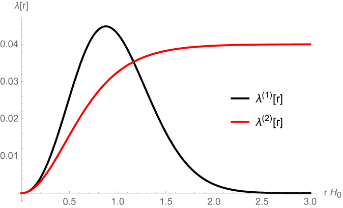
Figure 1: Plot of $\lambda^{(i)}(r)$ for the model (i=1) (7.15) with coefficients given in (7.26) and the model (i=2) (7.16) with coefficients given in (7.27).

In particular, for $\lambda^{\mbox{\tiny(1)}}(r)$ we have a bump at $r\sim r_{0}$, while for $\lambda^{\mbox{\tiny(2)}}(r)$ the perturbation start from zero and becomes a constant $\lambda_{0}$ far away. We imposed for both cases $\lambda^{\prime}(r=0)=0$ (see 6.18). The parameter $\lambda_{0}$ characterises the size of the void, $r_{0}$ and $\Delta$ characterise the transition to uniformity.

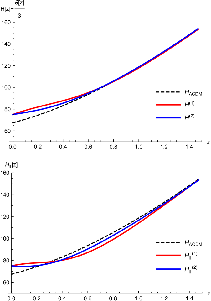
Figure 2: In the upper fig. we show the Hubble (volume expansion) parameter ${\cal H}=\frac{\theta}{3}$ (4.40) as a function of redshift for the $\Lambda$CDM model ${\cal H}_{\Lambda CDM}$ and for the models (1) ${\cal H}^{\mbox{\tiny(1)}}$(7.15) and (2) ${\cal H}^{\mbox{\tiny(2)}}$ (7.16). In the lower fig. we show the radial Hubble expansion rate (4.38, 6.15) always for the models (1) ${\cal H}_{\parallel}^{\mbox{\tiny(1)}}$(7.15) and (2) ${\cal H}_{\parallel}^{\mbox{\tiny(2)}}$ (7.16). The Hubble scale is expressed in ${\rm km\;s^{-1}\;Mpc^{-1}}$.

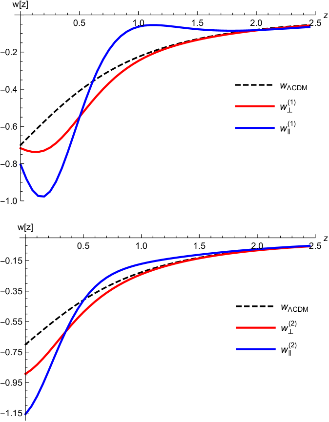
Figure 3: Effective equations of states relative to the FRW $\Lambda$CDM model $w_{\Lambda CDM}$, to the radial and transverse expansion rates $w_{\parallel/\perp}$ (7.5), for the models (1) (7.15) and (2) (7.16).

For the choice of the parameter space we impose the following constraints:

• Matching with the $\Lambda$CDM model in the early universe (as you can see from fig. 2, already present for $z\sim 1.5$), so we start with

  $$\left.{\cal H}_{\parallel}^{\mbox{\tiny(1,2)}}(z)\right|_{z\gg 1}=\left.{\cal H}_{\Lambda CDM}(z)\right|_{z\gg 1}\Rightarrow\quad H_{0}=H_{0}^{CMB}=67.4\;{\rm km\;s^{-1}\;Mpc^{-1}}$$ (7.17)

  as given by (6.15, 7.7, 6.21).

• then we tune the parameters, for model (1) (7.15) and model (2) (7.16) in such a way that $\lambda^{\mbox{\tiny(1)}^{\prime\prime}}\!(0)=\lambda^{\mbox{\tiny(2)}^{\prime\prime}}\!(0)$ in order to get the same value at $r=0$

  $${\cal H}^{\mbox{\tiny(1)}}_{\parallel}(z=0)={\cal H}^{\mbox{\tiny(2)}}_{\parallel}(z=0)=H_{0}\;(1+0.667\;\lambda^{\prime\prime}(0))=75\;{\rm km\;s^{-1}\;Mpc^{-1}}$$ (7.18)

  that implies

  $$\lambda(0)=\lambda^{\prime}(0)=0,\quad\lambda^{\prime\prime}(0)=0.17$$ (7.19)

Note the relationship

$$\rho(t_{0},r=0)=3\;H_{0}^{2}\;\left(1-0.074\;\lambda^{\prime\prime}(0)\right)\rightarrow\frac{{\cal H}_{\parallel}(0)-H_{0}}{H_{0}}\equiv\frac{\Delta H_{0}}{H_{0}}=-9.05\;\delta_{0}$$ (7.20)

where $\delta_{0}=\Delta\rho(t_{0},r=0)/\rho(t_{0},r=0)$ to be compared with the expression valid in a FRW universe for an adiabatic perturbation in density of our local spacetime [29, 30]

$$\frac{\Delta H_{0}}{H_{0}}=-\frac{1}{3}\;f(\Omega_{m})\;\delta_{0}$$ (7.21)

where $f(\Omega_{m})\sim 0.5$. A $9\%$ of shift for the Hubble constant (as observed) in a $\Lambda$CDM model implies $\delta^{\Lambda CDM}_{0}\sim 0.5$ while in our N$\Lambda$CDM model $\delta^{N\Lambda CDM}_{0}\sim 0.01$.
For the nearby effective equation of state (7.5) and the effective acceleration (7.6), we also get

$$w_{\parallel}(0)=-0.7-2.695\;\lambda^{\prime\prime}(0)+0.445\;\lambda^{\prime\prime\prime}(0)$$ (7.22)

$$w_{\perp}(0)=-0.7-1.140\;\lambda^{\prime\prime}(0)+0.222\;\lambda^{\prime\prime\prime}(0)$$ (7.23)

$$q(0)=-0.55-4.043\;\lambda^{\prime\prime}(0)+0.667\;\lambda^{\prime\prime\prime}(0)$$ (7.24)

A particular realisation of eq. (7.19) in the parameter space of (7.15) and (7.16) is given by

$$H_{0}=67.4\;{\rm km\;s^{-1}\;Mpc^{-1}},\;\Omega_{m}=0.3,\;\Omega_{\Lambda}=0.7,\;$$ (7.25)

$$model\;(1) : \quad r_{0}=0.5/H_{0},\;\Delta=0.8,\;\lambda_{0}=8\;10^{-2}$$ (7.26)

$$model\;(2) : \quad r_{0}=0.2/H_{0},\;\Delta=0.328,\;\lambda_{0}=4\;10^{-2}$$ (7.27)

as a result $\lambda^{\mbox{\tiny(1)}^{\prime\prime\prime}}(0)=0.793,\;\;\lambda^{\mbox{\tiny(2)}^{\prime\prime\prime}}(0)=0$ so that we get

$$w_{\parallel}^{\mbox{\tiny(1)}}(0)=-0.80,\quad w_{\perp}^{\mbox{\tiny(1)}}(0)=-0.72,\quad q^{\mbox{\tiny(1)}}(0)=-0.88,$$ (7.28)

$$w_{\parallel}^{\mbox{\tiny(2)}}(0)=-1.16,\quad w_{\perp}^{\mbox{\tiny(2)}}(0)=-0.89,\quad q^{\mbox{\tiny(2)}}(0)=-1.09$$ (7.29)

Note however that the full $z$ dependence of the above observables results quit not trivial as shown in figure 3 . Comparing with the prediction of $q_{0}=-1.08\pm 0.29$ [32], we see an interesting agreement with data (the local determination of the deceleration parameter for the standard $\Lambda$CDM model gives $q=-0.55$ for $\Omega_{m}=0.3$). For the future it will be interesting to provide a functional analysis that produces a best fit model for these observables. Here we have given a simple realisation of the model’s potential.

7.2 Geodesics for small $r$ expansion

In the small redshift expansion from eqs (7.1, 7.3) we get

$$a(z) = 1-z+\left(1-\frac{3}{4}\,\Omega_{\chi}+\frac{R_{2}^{\prime}(t_{0})-R_{2}(t_{0})}{2\,{\cal H}_{0}}\right)$$ (7.30)

$$t(z) = t_{0}-\frac{z}{{\cal H}_{0}}+\left(\frac{1}{2}-\Omega_{\chi}-\frac{3\;\Omega_{\mathit{m}}}{4}+\frac{R_{2}^{\prime}(t_{0})}{2\;{\cal H}_{0}^{2}}-\frac{R_{2}(t_{0})}{2\;{\cal H}_{0}}\right)\frac{z^{2}}{{\cal H}_{0}}+{\cal O}(z^{2}),$$ (7.31)

$$r(z) = \frac{z}{{\cal H}_{0}}+\left(\Omega_{\chi}-\frac{3\;\Omega_{\mathit{m}}}{4}-\frac{R_{2}^{\prime}(t_{0})}{2\;{\cal H}_{0}^{2}}\right)\frac{z^{2}}{{\cal H}_{0}}+{\cal O}(z^{2})$$ (7.32)

(where we used $\Omega_{\Lambda}=1-\Omega_{m}-\Omega_{\chi}$). We can parametrize the various corrections as functions of the expansion coefficients of the acceleration and shear functions, see eq. (6.26):

$${\cal A}(z) = {\cal H}_{0}\left({\cal A}_{1}\,z+{\cal A}_{2}\,\frac{z^{2}}{2}+...\right),\qquad{\Sigma}(z)={\cal H}_{0}\left({\Sigma}_{1}\,z+{\Sigma}_{2}\,\frac{z^{2}}{2}+...\right)$$ (7.33)

where ${\cal A}_{i}$ and ${\Sigma}_{i}$ are constants depending from the initial conditions and free parameters:

$${\cal A}_{1} = \frac{3}{2}\;\Omega_{\chi},\qquad{\Sigma}_{1}=\frac{1}{3\,{\cal H}_{0}}\;\left(R_{2}^{\prime}(t_{0})-R_{2}(t_{0})\right)$$ (7.34)

$${\cal A}_{2} = \frac{3\,\mathcal{A}_{1}\,\Sigma_{1}}{2}+\frac{\mathcal{A}_{1}^{2}}{3}+\frac{F_{3}\left(t_{0}\right)}{4\,\mathcal{H}_{0}^{3}}+\mathcal{A}_{1}\left(-\frac{3\,\Omega_{m}}{8}-1\right)-\frac{3\,\mathcal{A}_{1}\,R_{2}^{\prime}\left(t_{0}\right)}{4\,\mathcal{H}_{0}}$$ (7.35)

$${\Sigma}_{2} = -\frac{\mathcal{A}_{1}}{3}+\Sigma_{1}\left(\frac{\mathcal{A}_{1}}{6}+\frac{1}{8}\left(3\,\Omega_{m}+4\right)\right)+\frac{R_{3}^{\prime}\left(t_{0}\right)-Y_{3}(t_{0})}{9\,\mathcal{H}_{0}^{2}}-\frac{\Sigma_{1}\,R_{2}^{\prime}\left(t_{0}\right)+\frac{1}{6}\,R_{2}^{\prime\prime}\left(t_{0}\right)}{\mathcal{H}_{0}}+\frac{9\,\Sigma_{1}^{2}}{4}$$

Note that $R_{2}^{\prime}\left(t_{0}\right)$ (and also $R_{2}^{\prime\prime}\left(t_{0}\right),\;R_{3}^{\prime}\left(t_{0}\right)$) can be reads from eq. (F.1) as a function of the initial conditions $R_{2}\left(t_{0}\right)$ and the various parameters. From (7.4), the luminosity distance - redshift relationship can be parametrised in the usual way as

$$d_{L}(z) \equiv \frac{z}{{\cal H}_{0}}+\left(1-Q_{0}\right)\frac{z^{2}}{2\;{\cal H}_{0}}+{\cal O}(z^{3})$$ (7.36)

where we observe as the deceleration parameter $Q_{0}$, deduced by $d_{L}$, is different from the usual dynamical deceleration parameter $q_{0}=-\left.\frac{a^{\prime\prime}\;a}{(a^{\prime})^{2}}\right|_{t_{0}}$ [31]:

$$Q_{0} = -1+\frac{3}{2}\;\Omega_{m}-\frac{4}{3}\;{\cal A}_{1}+3\;\Sigma_{1},\qquad q_{0}=-1+\frac{3}{2}\;\Omega_{m}-\frac{{\cal A}_{1}}{3},\;\;$$

$$\qquad\qquad\qquad Q_{0}-q_{0}=-{\cal A}_{1}+3\;{\Sigma_{0}}$$

The radial Hubble parameter results

$${\cal H}_{\parallel}(z) = \mathcal{H}_{0}+\mathcal{H}_{0}\left(-\frac{4\,\mathcal{A}_{1}}{3}+\frac{3\,\Omega_{m}}{2}+3\,\Sigma_{1}\right)\,z+$$

$$z^{2}\left(-\frac{1}{4}\,R_{2}^{\prime\prime}\left(t_{0}\right)+{\cal H}_{0}\,\left(-\frac{2\,\mathcal{A}_{1}^{2}}{9}-2\,\mathcal{A}_{2}+\Sigma_{1}\,\left(\frac{3\,\mathcal{A}_{1}}{4}+\frac{3}{16}\,\left(4-9\,\Omega_{m}\right)\right)+\right.\right.$$

$$\left.\left.\mathcal{A}_{1}\,\left(\frac{5\,\Omega_{m}}{4}+\frac{1}{3}\right)+\frac{3}{8}\left(4-3\,\Omega_{m}\right)\,\Omega_{m}-\frac{9\,\Sigma_{1}^{2}}{8}+\frac{9\,\Sigma_{2}}{2}\right)\right)+...$$

and the difference with the orthogonal Hubble rate (4.39) is

$${\cal H}_{\parallel}(z)-{\cal H}_{\perp}(z)={\cal H}_{0}\left(z\,\left(\frac{3\,\Sigma_{1}}{2}-\mathcal{A}_{1}\right)+z^{2}\,\left(3\,\Sigma_{2}-2\,\mathcal{A}_{2}\right)+...\right)$$ (7.39)

Finally the effective radial and angular equations of state (7.5) at leading order ${\cal O}(z)$ result

$$w_{\perp}(z) = -1+\Omega_{m}-\frac{2}{9}\;{\cal A}_{1}+\Sigma_{1}+...,$$ (7.40)

$$w_{\parallel}(z) = -1+\Omega_{m}-\frac{8}{9}\;{\cal A}_{1}+2\;\Sigma_{1}+\left(-\frac{40\,\mathcal{A}_{1}^{2}}{27}-\frac{8\,\mathcal{A}_{2}}{3}+\mathcal{A}_{1}\left(\frac{1}{9}\left(39\,\Omega_{m}-4\right)+\frac{19\,\Sigma_{1}}{3}\right)+\right.$$ (7.41)

$$\left.\Sigma_{1}\left(3-\frac{33\,\Omega_{m}}{4}\right)-3\,\Omega_{m}^{2}+3\,\Omega_{m}-\frac{R_{2}^{\prime\prime}\left(t_{0}\right)}{3\,\mathcal{H}_{0}}-\frac{15\,\Sigma_{1}^{2}}{2}+6\,\Sigma_{2}\right)\,z+...$$

Comparing with the prediction of [32], where the estimations only use supernovae in the redshift range $0.023\leq z\leq 0.15$, that gives ${\cal H}_{0}=75.35\pm 1.68\;km\,s^{-1}\,Mpc^{-1}$ and $Q_{0}=-1.08\pm 0.29$ we can estimate the nearby equation of state, the acceleration and the $\Omega_{\chi}$ parameter to

$$w_{\parallel}=-1.05\pm 0.19+\left(6\,\Sigma_{2}-\frac{8\,\mathcal{A}_{2}}{3}-\frac{Y_{2}^{\prime\prime}(t_{0})}{3\,{\cal H}_{0}}-\frac{3\,\Sigma_{1}^{2}}{4}+(0.73\pm 0.14)+(2.32\pm 0.07)\,\Sigma_{1}\right)z$$

$${\cal A}_{1}=0.40\pm 0.22+\frac{9}{4}\,\Sigma_{1},\qquad\Omega_{\chi}=0.27\pm 0.15+\frac{3}{2}\,\Sigma_{1}$$ (7.42)

To disentangle the degeneracy ${\cal A}_{1}-\Sigma_{1}$ we need an extra independent cosmographic measure that can be the redshift drift, as suggested in [28].

8 Conclusions

We analysed an adiabatic perfect fluid cosmological model characterised by two terms into the Lagrangian (3.1), one featuring a CC and another a DM component, both terms are builded with the same field content (goldstone modes of the spontaneously broken space and time) (2.1). In this sense we have a single fluid mimicking both DE and DM. The presence of a space dependent CC results thermodynamically related to the conserved (in time) entropy density (3.10). Such a DE component breaks the homogeneity of the space time and induces a non trivial space dependence for the pressure (3.3) such that the comoving observers are not anymore geodesic ${\cal A}_{\mu}\neq 0$ (3.10).
We study the equation of motion of such a system using a 1+1+2 formalism where we use two background vectors: one is time-like $u^{\mu}$ (the geodesic of the fluid) and the other is space-like $v^{\mu}$ (proportional to the non zero acceleration) (4.5).
In chapter (4) we give all the covariant equation for a LRS space (4.15, 4.16, 4.17, 4.18, 4.19) and part of some non perturbative solutions (4.25).
In chapter (4.1) we give the eqs for the propagation of light bundles and we stress the difference in between the radial ${\cal H}_{\parallel}$ and transverse ${\cal H}_{\perp}$ expansion rates (4.38, 4.39).
In chapter (5) we study the eqs of motion in a comoving coordinate system using a rotationally invariant Lema$\hat{\rm i}$tre metric (5.1) characterized by three form factors functions of the $t,\,r$ variables $(F(t,r),\,X(t,r),\,R(t,r))$. The eqs of motion (6.6) are solved in two limiting cases.
In chapter (6.1) we perturb a FRW background with a small $r$-dependent cosmological constant (6.9) while in chapter (7.1) we give the corresponding solutions of the null geodesics.
In chapter (6.2) instead we study the solutions to (6.6) in the small $r\,H_{0}\ll 1$ expansion regime and in chapter (7.2) we give the corresponding null geodesic paths.
As observable, to check the outcome of our model, we study the luminosity distance $d_{L}$ (7.4), the effective eqs of state along the radial and transverse direction $w_{\parallel,\perp}$ (7.5) computed along the light of sight. In chapter (7.1) we analyse two kinds of CC $r$-profiles (7.15,7.16) and we report our main results in fig. 2 and 3.
In chapter (7.2) the small $r$ expansion is translated in a small $z$ redshift expansion where we can extract the deceleration parameter $Q_{0}$ (7.36) as a function of constants describing the background evolution. It is interesting to note as, in such a limit, the background Hubble law (6.24) shows the presence of an extra matter component $\Omega_{\chi}$ (proportional to the local acceleration parameter (7.34)) whose equation of state result $w_{\chi}=-4/3$.
To simplify our computations we put the observer at the center of the void region violating the Copernican (Cosmological) Principle. Our model represent an alternative to the more popular spherically symmetric LTB model where the matter component of the universe is the responsible of the inhomogeneity. Assuming the $\Lambda$CDM model, at present, the discrepancy between the Hubble values measured around local distance ladders and from CMB Planck data (see [35], [36] for a full reference list) has reached the 4-6 $\sigma$ level. This model represents a minimal modification to the $\Lambda$CDM scenario (for this reason we named next to minimal $\Lambda$CDM model (N$\Lambda$CDM)) able to modify the null geodesic paths in agreement with present data. This paper is dedicated to the theoretical analysis of the model therefore we have not carried out a statistical analysis for the best possible parameter space of the model by just analysed two generic possible space dependent shapes for the CC shown in fig.1 The first kind of shape is featuring a bump of $\Lambda(r)$, while the second one a smooth increase of $\Lambda(r)$ till a constant value. Choosing appropriate parameters we first adjust the discrepancy for the Hubble parameter nearby and far away (Planck), then we cheque the implications for the effective equations of state. For example we note that data favors the second model where an effective nearby equation of state $w\leq-1$ is obtained mimicking a phantom dark energy component [37] . Following the classification mechanism solutions for the $H_{0}$-crisis [35], we see that this kind of models can be inserted in the class of the alternative proposals operating at late time: Local Inhomogeneity. It is clear that to probe this kind of radial inhomogeneity around us we further have to do many other test: CMB spectral distortions, BAO, type Ia supernovae, cosmic chronometers, ect. as is in progress for the $\Lambda$CDM model [38].

Appendix A 1+3 and 1+1+2 Formalism

• 1+3 Formalism
  Projection tensor on the metric of the 3-space (S) orthogonal to $u^{\alpha}$

  $$h_{\alpha\beta}=g_{\alpha\beta}+u_{\alpha}\;u_{\beta},\qquad h^{\alpha}_{\alpha}=3$$ (A.1)

  Any 3-vector, $V^{\alpha}$, can be irreducibly split into a component along $u^{\alpha}$ and a sheet component ${\cal V}^{\alpha}$, orthogonal to $u^{\alpha}$

  $$V^{\alpha}=V\;u^{\alpha}+{\cal V}^{\alpha},\qquad V=-V_{\alpha}\;u^{\alpha},\quad{\cal V}^{\alpha}=h^{\alpha}_{\beta}\;V^{\beta}$$ (A.2)

  The covariant derivative of a scalar function $f$ projected along $u^{\alpha}$ is so defined

  $$\dot{f}=u^{\alpha}\nabla_{\alpha}f$$ (A.3)

  We are now able to decompose the covariant derivative of $u^{\alpha}$ orthogonal to $u^{\alpha}$ giving

  $$\nabla_{\alpha}\;u_{\beta}=-u_{\alpha}\;{\cal A}_{\beta}+\frac{1}{3}\;\theta\;h_{\alpha\beta}+\sigma_{\alpha\beta}+\omega_{\beta\alpha}$$ (A.4)

  • 4-Acceleration

    $${\cal A}_{\alpha}\equiv u^{\beta}\nabla_{\beta}\;u_{\alpha}\equiv\dot{u}_{\alpha}$$ (A.5)

  • Expansion

    $$\theta\equiv\nabla^{\alpha}\;u_{\alpha}$$ (A.6)

  • Shear

    $$\sigma_{\alpha\beta}=h^{\lambda}_{\beta}\;\nabla_{(\lambda}\;u_{\rho)}\;h_{\alpha}^{\rho}-\frac{1}{3}\;\theta\;h_{\alpha\beta}$$ (A.7)

  • Vorticity

    $$\omega_{\alpha\beta}=h^{\lambda}_{\beta}\;\nabla_{[\lambda}\;u_{\rho]}\;h_{\alpha}^{\rho},\qquad\omega^{\alpha}=\epsilon^{\alpha\beta\gamma}\;\omega_{\beta\gamma}$$ (A.8)

  The decomposition defined above is also used to define a set of derivatives operators acting on various kind of tensors:

  $$\dot{X}^{\alpha..\beta}_{\gamma..\delta}=u^{\lambda}\;\nabla_{\lambda}\;X^{\alpha..\beta}_{\gamma..\delta}$$ (A.9)

  $$D_{\lambda}X^{\alpha..\beta}_{\gamma..\delta}=h^{\lambda_{1}}_{\lambda}\;h^{\alpha}_{\alpha_{1}}\;h^{\beta}_{\beta_{1}}\;...\;h^{\gamma}_{\gamma_{1}}\;h^{\delta}_{\delta_{1}}\;\nabla_{\lambda_{1}}\;X^{\alpha_{1}..\beta_{1}}_{\gamma_{1}..\delta_{1}}$$ (A.10)

• 1+1+2 Formalism
  The 1 + 1 + 2 approach is based on a double foliation of the spacetime: a given manifold is first foliated in spacelike 3-surfaces and then these 3-surfaces are foliated in 2 surfaces. These foliations are obtained by defining a congruence of integral curves of the time-like ($u^{\alpha}\;u_{\alpha}=-1$) vector field $u^{\alpha}$ and a congruence of integral curves defined by the spacelike ($v^{\alpha}\;v_{\alpha}=1$) vector $v^{\alpha}$.
  Projection tensor which represents the metric of the 2-spaces (W) orthogonal to $u^{\alpha}$ and $v^{\alpha}$.

  $$N_{\alpha\beta}=h_{\alpha\beta}-v_{\alpha}\;v_{\beta},\qquad N^{\alpha}_{\alpha}=2$$ (A.11)

  Any 3-vector $V^{\alpha}$ can be irreducibly split into a component along $v^{\alpha}$ and a sheet component ${\bf V}^{\alpha}$, orthogonal to $v^{\alpha}$ and $u^{\alpha}$.

  $$V^{\alpha}=V\;v^{\alpha}+{\bf V}^{\alpha},\qquad V=V_{\alpha}\;v^{\alpha},\quad{\bf V}^{\alpha}=N^{\alpha}_{\beta}\;V^{\beta}$$ (A.12)

  The decomposition defined above can be also used to define a set of derivatives operators:

  $$\hat{X}^{\alpha..\beta}_{\gamma..\delta}=v^{\lambda}\;\nabla_{\lambda}\;X^{\alpha..\beta}_{\gamma..\delta}$$ (A.13)

  $$\delta_{\lambda}X^{\alpha..\beta}_{\gamma..\delta}=N^{\lambda_{1}}_{\lambda}\;N^{\alpha}_{\alpha_{1}}\;h^{\beta}_{\beta_{1}}\;...\;N^{\gamma}_{\gamma_{1}}\;N^{\delta}_{\delta_{1}}\;\nabla_{\lambda_{1}}\;X^{\alpha_{1}..\beta_{1}}_{\gamma_{1}..\delta_{1}}$$ (A.14)

  The hat-derivative is the derivative along the vector field $v^{\alpha}$ in the surfaces orthogonal to $u^{\alpha}$, for a scalar function $f$ we have the definitions

  $$\hat{f}=v^{\alpha}\nabla_{\alpha}f$$ (A.15)

  For the mixed double derivative we have the relationship

  $$\hat{\dot{f}}-\dot{\hat{f}}=-{\cal A}\;\dot{f}+\left(\frac{\theta}{3}+\Sigma\right)\;\hat{f}$$ (A.16)

  We are now able to decompose the covariant derivative of $v^{\alpha}$ orthogonal to $u^{\alpha}$ giving

  $$\nabla_{\alpha}\;u_{\beta}=-{\cal A}\;u_{\alpha}\;e_{\beta}+\left(\frac{\theta}{3}+\Sigma\right)\;v_{\alpha}\;v_{\beta}+\left(\frac{\theta}{3}-\frac{\Sigma}{2}\right)\;N_{\alpha\beta}+\Omega\;\epsilon_{\alpha\beta}$$ (A.17)

  $$\nabla_{\alpha}\;v_{\beta}=-{\cal A}\;u_{\alpha}\;u_{\beta}+\left(\frac{\theta}{3}+\Sigma\right)\;v_{\alpha}\;u_{\beta}+\frac{\phi}{2}\;N_{\alpha\beta}+\xi\;\epsilon_{\alpha\beta}$$ (A.18)

  $$D_{\alpha}\;v_{\beta}=v_{\beta}\;a_{\beta}+\frac{1}{2}\;\phi\;N_{\alpha\beta}+\xi\;\epsilon_{\alpha\beta}+\zeta_{\alpha\beta}$$ (A.19)

  where

  • Sheet expansion

    $$\phi=\delta_{\alpha}\;v^{\alpha}=D_{\alpha}\;v^{\alpha}$$ (A.20)

  • Twisting of the sheet (the rotation of $v^{\alpha}$)

    $$\xi=\frac{1}{2}\epsilon^{\alpha\beta}\;\delta_{\alpha}v_{\beta}$$ (A.21)

  • Acceleration of $v^{\alpha}$

    $$a_{\alpha}=\hat{v}_{\alpha}$$ (A.22)

  • Shear of $v^{\alpha}$

    $$\zeta_{\alpha\beta}=\delta_{\{\alpha}\;v_{\beta\}}$$ (A.23)

  Note the following identities/definitions

  $$v\cdot u=0,\quad v^{2}=1,\quad v\cdot a=-u\cdot\dot{v},\quad v\cdot\dot{v}=0$$ (A.24)

  $${\cal A}={\cal A}^{\alpha}v_{\alpha}=-u^{\alpha}\;\dot{v}_{\alpha},\quad\Sigma=v^{\alpha}\sigma_{\alpha\beta}v^{\beta},\quad\Omega=v^{\alpha}\omega_{\alpha\beta}v^{\beta},\quad$$ (A.25)

  $${\cal E}=v^{\alpha}E_{\alpha\beta}v^{\beta},\quad{\cal H}=v^{\alpha}H_{\alpha\beta}v^{\beta},\quad$$ (A.26)

  where $E_{\alpha\beta}$ and $H_{\alpha\beta}$ are the electric and the magnetic part of the Weyl tensor respectively.

Appendix B Thermodynamical stability

Stable equilibrium is constraining the second order variations of the thermodynamical potentials, specifically we have

$$\delta^{2}S\leq 0\quad{\rm or}\quad\delta^{2}E\geq 0$$ (B.1)

For a more formal contact with the thermodynamical formalism we can define in a field theoretical framework some classical text book quantities [33]:

• Specific heat at constant volume

  $$C_{V}=T\;\left.\frac{\partial S}{\partial T}\right|_{V,N}=V\;T\;U_{Y^{2}}$$ (B.2)

• Specific heat at constant pressure

  $$C_{p}=T\;\left.\frac{\partial S}{\partial T}\right|_{p,N}=V\;T\;\left(U_{Y^{2}}-\frac{(b\;U_{bY}-U_{Y})^{2}}{b^{2}\;U_{b^{2}}}\right)$$ (B.3)

• Coefficient of thermal expansion

  $$\alpha=\frac{1}{V}\;\left.\frac{\partial V}{\partial T}\right|_{p,N}=sign[T]\;\frac{(b\;U_{bY}-U_{Y})}{b^{2}\;U_{b^{2}}}$$ (B.4)

• Coefficient of isothermal compressibility

  $$\kappa_{T}=-\frac{1}{V}\;\left.\frac{\partial V}{\partial p}\right|_{T,N}=-\frac{1}{b^{2}\;U_{b^{2}}}$$ (B.5)

• Coefficient of adiabatic compressibility

  $$\kappa_{S}=-\frac{1}{V}\;\left.\frac{\partial V}{\partial p}\right|_{S,N}=-\frac{U_{Y^{2}}}{b^{2}\;U_{b^{2}}\;U_{Y^{2}}-(b\;U_{bY}-U_{Y})^{2}}$$ (B.6)

All of them satisfy the above relations

$$c_{p}-c_{V}=\frac{T\;\alpha^{2}}{\kappa_{T}},\qquad c_{p}\;\kappa_{S}=c_{V}\;\kappa_{T}$$ (B.7)

where $C_{p,V}\equiv V\;c_{p,V}$. Working with densities, thermodynamical stability requires the $|s_{ij}|$ matrix

$$s_{ij}=\begin{pmatrix}\frac{\partial^{2}s}{\partial\rho^{2}}&\frac{\partial^{2}s}{\partial\rho\partial n}\\ \frac{\partial^{2}s}{\partial\rho\partial n}&\frac{\partial^{2}s}{\partial n^{2}}\end{pmatrix}$$ (B.8)

to be negative defined so that

$$s_{\rho\rho}=-\frac{1}{T^{2}\,c_{V}}<0,\quad\det|s_{ij}|=\frac{1}{n^{2}\;T^{3}\,c_{V}\;\kappa_{T}}>0$$ (B.9)

$${\rm or}\quad c_{V}>0\qquad\&\qquad T\;\kappa_{T}>0$$ (B.10)

and also $c_{p}>c_{V}>0$ or $T\;\kappa_{T}\;c_{V}>0$ bringing to the following constraint for the potential

$$\frac{U_{Y^{2}}}{U_{b^{2}}}<0$$ (B.11)

Note that such a conditions are non perturbative and background independent.

Appendix C Cosmological Constant and $\Lambda$-Media

The largest symmetry inside the internal scalar space is a full unitary Diffeomorphism transformation

$$\Phi^{A}\to f^{A}(\Phi^{B})\;\;\;{\rm where}\;\;\;\det\left|\frac{\partial f^{A}}{\partial\Phi^{B}}\right|=1$$ (C.1)

whose feature is to select one specific invariant operator $Z$ that results the building block for a thermodynamical non trivial CC:

$$Z\equiv b\;Y=\frac{det|\Phi^{A}_{\alpha}|}{\sqrt{g}}=\frac{e^{\alpha\beta\gamma\delta}}{\sqrt{g}}\;e_{ABCD}\;\Phi^{A}_{\alpha}\;\Phi^{B}_{\beta}\;\Phi^{C}_{\gamma}\;\Phi^{D}_{\delta}$$ (C.2)

where $e^{\alpha\beta\gamma\delta}$ and $e_{ABCD}$ are the permutation tensors in the 4-Dim space-time and the 4-Dim scalar space.
The action generating an effective CC perfect fluid results (that we named $\Lambda$-Media in [13, 5])

$$S_{\Lambda}=\int d^{4}x\;\sqrt{g}\;\;U(Z)$$ (C.3)

The eqs of motion for the $\Phi^{A}$ scalar fields (for $U^{\prime\prime}\neq 0$) are given by

$$\nabla_{\mu}\;det|\Phi^{A}_{\alpha}|=0\quad\to\quad\Psi_{A}^{\alpha}\;\Phi^{A}_{\alpha\mu}=0\;\;\;{\rm where}\;\;\;\Psi_{A}^{\alpha}=\frac{\partial x^{\alpha}}{\partial\Phi^{A}}$$ (C.4)

($\Psi_{A}^{\alpha}\;\Phi^{A}_{\beta}=\delta^{\alpha}_{\beta},\;\;\Psi_{A}^{\alpha}\;\Phi^{B}_{\alpha}=\delta^{A}_{B}$) and imply the exact non perturbative solution

$$\nabla_{\mu}\;Z=0\quad\to\quad Z=Z_{0}\;\;{\rm constant\;in\;space\;and\;time}$$ (C.5)

The corresponding Energy Momentum Tensor (EMT) can be easily obtained

$$T_{\mu\nu}=(U-Z\;U^{\prime})\;g_{\mu\nu}\equiv-\Lambda\;g_{\mu\nu}$$ (C.6)

so that we have an effective CC: $\Lambda=(-U+Z\;U^{\prime})$. For such a model we can write the energy density $\rho$, the pressure $p$ and the entropy per particle $\sigma$ as [5]

$$\rho_{\Lambda}=-p_{\Lambda}=\Lambda,\;\;\;\sigma_{\Lambda}=\frac{s_{\Lambda}}{b}=U^{\prime}$$ (C.7)

Using the thermodynamical analysis of the previous chapter, for the specific potentials $U=U(b\;Y)$, we get that Perfect Fluid $\Lambda$-media are thermodynamically unstable. In fact we get

$$c_{V}=T\;b^{2}\;U^{\prime\prime},\qquad\kappa_{T}=-\frac{1}{b^{2}\;T^{2}\;U^{\prime\prime}},\qquad T\;c_{V}\;\kappa_{T}=-1$$ (C.8)

violating eq.(B.11). Note the paradox that dynamically the system is frozen to and exact de Sitter phase with no runaway solutions for the energy/entropy observables.

Appendix D Mixed derivatives for thermodynamical quantities

We give the mixed derivatives (A.16) for the thermodynamical quantities $\rho,\;p,\;\sigma$ for a perfect fluid

$$\hat{\dot{\rho}}-\dot{\hat{\rho}}={\cal A}\;\theta\;(\rho+p)+\left(\frac{\theta}{3}+\Sigma\right)\,\hat{\rho}$$ (D.1)

$$\hat{\dot{p}}-\dot{\hat{p}}=-{\cal A}\;\dot{p}-\left(\frac{\theta}{3}+\Sigma\right)\,{\cal A}\;(\rho+p)$$ (D.2)

$$\dot{\hat{\sigma}}=-\left(\frac{\theta}{3}+\Sigma\right)\,\hat{\sigma}$$ (D.3)

Appendix E Evolution equation for the radial form factor in almost FRW

In order to get a single evolution equation for the radial form factor of the metric $R(t,r)$ we can insert eq. (5.14) in (5.13) so we get $F$ as a function of $R$

$$F^{2} = \frac{9\;\mathbf{n}^{2}\;R\;\left(R^{(1,0)}\right)^{2}}{R\;\left(\mathbf{m}^{\prime}+R^{3}\;\Lambda^{\prime}\right)^{2}+3\;\mathbf{n}^{2}\left(\mathbf{m}+\Lambda\;R^{3}-3\;R\right)}$$ (E.1)

Finally to have a self contained eq. for $R$ we insert (E.1) inside (5.18)

$$\frac{R^{(1,1)}}{R^{(1,0)}}\;\left(R\;\left(\mathbf{m}^{\prime}+R^{3}\;\Lambda^{\prime}\right)+\frac{3\;\mathbf{n}^{2}\;\left(\mathbf{m}+\Lambda\;R^{3}-3\;R\right)}{\mathbf{m}^{\prime}+R^{3}\;\Lambda^{\prime}}\right)-$$ (E.2)

$$\;\left(R^{3}\;\Lambda^{\prime\prime}+\mathbf{m}^{\prime\prime}\right)\;R-\frac{3}{2}\;\mathbf{n}^{2}+\frac{R\;\mathbf{n}^{\prime}\;\left(\mathbf{m}^{\prime}+R^{3}\;\Lambda^{\prime}\right)}{\mathbf{n}}+$$

$$R^{(0,1)}\;\left(-6\;R^{3}\;\Lambda^{\prime}-\frac{3\;\mathbf{n}^{2}\left(\mathbf{m}^{\prime}\;\left(\Lambda\;R^{3}-1/2\;\mathbf{m}\right)+R^{3}\;\Lambda^{\prime}\;\left(15/6\;\mathbf{m}+4\;\Lambda\;R^{3}-9\;R\right)\right)}{R\;\left(\mathbf{m}^{\prime}+R^{3}\;\Lambda^{\prime}\right)^{2}}\right)=0$$

Appendix F Evolution equation for the radial form factors in small $r$ regime

Evolution for the form factor $R_{2,3}(t)$ where $R(t,r)=a(t)\,r+R_{2}(t)\,\frac{r^{2}}{2}+R_{3}(t)\,\frac{r^{3}}{6}+...$. We prefer to shift the derivation, from the variable $t$ to $a(t)$ (6.24) such that $f^{\prime}(t)=a\;\bar{\cal H}(a)\;f^{\prime}(a)$.

$$R_{2}^{\prime}(a)=\frac{{\cal H}_{0}^{2}\,R_{2}(a)\,\left(2\,a^{3}\,\Omega_{\Lambda}+3\,a^{4}\,\Omega_{\chi}-\Omega_{m}\right)}{2\,a^{4}\,\bar{\cal H}(a)^{2}}+\frac{\mathbf{m}_{4}\left(3\,\Omega_{m}-4\,a^{4}\,\Omega_{\chi}\right)}{216\,a^{3}\,\bar{\cal H}(a)^{2}\,\Omega_{m}}+\frac{a\,\ell_{3}}{3\,\bar{\cal H}(a)^{2}\,\Omega_{m}}$$ (F.1)

$$R_{3}^{\prime}(a) =-\frac{{\cal H}_{0}^{2}\,R_{3}(a)\left(-2\,a^{3}\,\Omega_{\Lambda}-3\,a^{4}\,\Omega_{\chi}+\Omega_{m}\right)}{2\,a^{4}\,\bar{\cal H}(a)^{2}}+\frac{{\cal H}_{0}^{2}\,\ell_{3}\,R_{2}(a)\left(a^{3}\,\left(3\,a\,\Omega_{\chi}+4\,\Omega_{\Lambda}\right)+7\,\Omega_{m}\right)}{4\,a^{3}\,\bar{\cal H}(a)^{4}\,\Omega_{m}}+$$ (F.2)

$$\frac{{\cal H}_{0}^{4}\,R_{2}(a){}^{2}\,\left(3\,a^{7}\,\Omega_{\chi}\,\left(3\,a\,\Omega_{\chi}+4\,\Omega_{\Lambda}\right)+6\,a^{3}\,\Omega_{m}\left(11\,a\,\Omega_{\chi}+6\,\Omega_{\Lambda}\right)+9\,\Omega_{m}^{2}\right)}{16\,a^{8}\,\bar{\cal H}(a)^{4}}-\frac{a^{2}\,\ell_{3}^{2}}{12\,\bar{\cal H}(a)^{4}\,\Omega_{m}^{2}}+$$

$$\frac{1}{\bar{\cal H}(a)^{2}}\left(\frac{3}{4}\,H_{0}^{4}\,\Omega_{\chi}\left(a^{3}\,\left(7\,a\,\Omega_{\chi}+6\,\Omega_{\Lambda}\right)+9\,\Omega_{m}\right)+\frac{a\,\ell_{4}}{3\,\Omega_{m}}\right)$$

where we used $\Lambda_{i}\equiv 3\;{\cal H}_{0}^{2}\;{\ell}_{i}$.

References

- [1] N. Aghanim et al. [Planck Collaboration], arXiv:1807.06209 [astro-ph.CO].
- [2] P. J. E. Peebles and B. Ratra, Astrophys. J. Lett. 325 (1988), L17 doi:10.1086/185100
- [3] H. A. P. Macedo, L. S. Brito, J. F. Jesus and M. E. S. Alves, [arXiv:2305.18591 [astro-ph.CO]].
- [4] J. V. Narlikar, J. C. Pecker and J. P. Vigier, J. Astrophys. Astron. 12 (1991), 7–16 doi:10.1007/BF02709768
- [5] M. Celoria, D. Comelli and L. Pilo, JCAP 01 (2019), 057 doi:10.1088/1475-7516/2019/01/057 [arXiv:1712.04827 [gr-qc]].
- [6] M. Celoria, D. Comelli and L. Pilo, JCAP 1709 (2017) no.09, 036 doi:10.1088/1475-7516/2017/09/036 [arXiv:1704.00322 [gr-qc]].
- [7] G. F. R. Ellis and H. van Elst, NATO Sci. Ser. C 541 (1999) 1 [gr-qc/9812046].
-
[8]
G. F. R. Ellis,
J. Math. Phys. 8 (1967) 1171.
doi:10.1063/1.1705331.
J. M. Stewart and G. F. R. Ellis, J. Math. Phys. 9 (1968) 1072. doi:10.1063/1.1664679.
H. van Elst and G. F. R. Ellis, Class. Quant. Grav. 13 (1996) 1099 [gr-qc/9510044]. - [9] K. Bolejko and P. Lasky, Mon. Not. Roy. Astron. Soc. 391 (2008), 59 doi:10.1111/j.1745-3933.2008.00555.x [arXiv:0809.0334 [astro-ph]]
- [10] H. Alnes and M. Amarzguioui, Phys. Rev. D 74 (2006), 103520 doi:10.1103/PhysRevD.74.103520 [arXiv:astro-ph/0607334 [astro-ph]].
- [11] C. Clarkson, Comptes Rendus Physique 13 (2012), 682-718 doi:10.1016/j.crhy.2012.04.005 [arXiv:1204.5505 [astro-ph.CO]].
-
[12]
Carter, B., Quintana, H. (1972) Foundations of general relativistic high pressure elasticity theory. Proc. R. Soc. Lond. A331, p. 57-83.
Carter, B. (1980) Rheometric structure theory, convective differentiation and continuum electrodynamics. Proc. R. Soc. Lond. A372, p. 169-200.
N. Andersson and G. L. Comer, Living Rev. Rel. 10 (2007) 1 doi:10.12942/lrr-2007-1 [gr-qc/0605010]. - [13] G. Ballesteros, D. Comelli and L. Pilo, Phys. Rev. D 94 (2016) no.12, 124023 doi:10.1103/PhysRevD.94.124023 [arXiv:1603.02956 [hep-th]].
- [14] G. Ballesteros, D. Comelli and L. Pilo, Phys. Rev. D 94 (2016) no.2, 025034 doi:10.1103/PhysRevD.94.025034 [arXiv:1605.05304 [hep-th]].
- [15] H. Kodama and M. Sasaki, Prog. Theor. Phys. Suppl. 78 (1984) 1. doi:10.1143/PTPS.78.1
- [16] M. Celoria, D. Comelli and L. Pilo, JCAP 1803 (2018) no.03, 027 doi:10.1088/1475-7516/2018/03/027 [arXiv:1711.01961 [gr-qc]].
- [17] P. K. Aluri, P. Cea, P. Chingangbam, M. C. Chu, R. G. Clowes, D. Hutsemékers, J. P. Kochappan, A. M. Lopez, L. Liu and N. C. M. Martens, et al. Class. Quant. Grav. 40 (2023) no.9, 094001 doi:10.1088/1361-6382/acbefc [arXiv:2207.05765 [astro-ph.CO]].
- [18] D. Wands, J. De-Santiago and Y. Wang, Class. Quant. Grav. 29 (2012) 145017 doi:10.1088/0264-9381/29/14/145017 [arXiv:1203.6776 [astro-ph.CO]].
- [19] Krasinski A. 1997 Inhomogeneous Cosmological Models (Cambridge: Cambridge University Press)
-
[20]
C. A. Clarkson and R. K. Barrett,
Class. Quant. Grav. 20 (2003) 3855
doi:10.1088/0264-9381/20/18/301
[gr-qc/0209051].
G. Betschart and C. A. Clarkson, Class. Quant. Grav. 21 (2004) 5587 doi:10.1088/0264-9381/21/23/018 [gr-qc/0404116].
C. Clarkson, Phys. Rev. D 76 (2007) 104034 doi:10.1103/PhysRevD.76.104034 [arXiv:0708.1398 [gr-qc]].
S. Carloni and D. Vernieri, Phys. Rev. D 97 (2018) no.12, 124056 doi:10.1103/PhysRevD.97.124056 [arXiv:1709.02818 [gr-qc]]. -
[21]
S. Singh, G. F. R. Ellis, R. Goswami and S. D. Maharaj,
Phys. Rev. D 94 (2016) no.10, 104040
doi:10.1103/PhysRevD.94.104040
[arXiv:1609.03288 [gr-qc]].
S. Singh, G. F. R. Ellis, R. Goswami and S. D. Maharaj, Phys. Rev. D 96 (2017) no.6, 064049 doi:10.1103/PhysRevD.96.064049 [arXiv:1707.06407 [gr-qc]].
S. Singh, R. Goswami and S. D. Maharaj, arXiv:1805.05664 [gr-qc]. - [22] R. Jimenez, R. Maartens, A. R. Khalifeh, R. R. Caldwell, A. F. Heavens and L. Verde, JCAP 05 (2019), 048 doi:10.1088/1475-7516/2019/05/048 [arXiv:1902.11298 [astro-ph.CO]].
- [23] C. Alcock and B. Paczynski, Nature 281 (1979) 358. doi:10.1038/281358a0
- [24] V. Marra and M. Paakkonen, JCAP 01 (2012), 025 doi:10.1088/1475-7516/2012/01/025 [arXiv:1105.6099 [gr-qc]].
- [25] G. Lemaitre, Gen. Rel. Grav. 29 (1997) 641 [Annales Soc. Sci. Bruxelles A 53 (1933) 51]. doi:10.1023/A:1018855621348.
- [26] A. A. H. Alfedeel and C. Hellaby, Gen. Rel. Grav. 42 (2010), 1935-1952 doi:10.1007/s10714-010-0971-y [arXiv:0906.2343 [gr-qc]].
- [27] P. D. Lasky and K. Bolejko, Class. Quant. Grav. 27 (2010) 035011 doi:10.1088/0264-9381/27/3/035011 [arXiv:1001.1159 [astro-ph.CO]].
- [28] M. H. Partovi and B. Mashhoon, Astrophys. J. 276 (1984) 4. doi:10.1086/161588
- [29] Turner, Edwin L. and Cen, Renyue and Ostriker, Jeremiah P. The Astronomical Journal (1992) 103, 5,1427 doi : 10.1086/116156 https://ui.adsabs.harvard.edu/abs/1992AJ….103.1427T
- [30] V. Marra, L. Amendola, I. Sawicki and W. Valkenburg, Phys. Rev. Lett. 110 (2013) no.24, 241305 doi:10.1103/PhysRevLett.110.241305 [arXiv:1303.3121 [astro-ph.CO]].
- [31] J. F. Pascual-Sanchez, Mod. Phys. Lett. A 14 (1999), 1539-1544 doi:10.1142/S0217732399001632 [arXiv:gr-qc/9905063 [gr-qc]].
- [32] D. Camarena and V. Marra, Phys. Rev. Res. 2 (2020) no.1, 013028 doi:10.1103/PhysRevResearch.2.013028 [arXiv:1906.11814 [astro-ph.CO]].
- [33] H. B. Callen, Thermodynamics and an Introduction to Thermostatistics, 2nd Edition, John Wiley and Sons, New York, 1960.
- [34] J. Garcia-Bellido and T. Haugboelle, JCAP 04 (2008), 003 doi:10.1088/1475-7516/2008/04/003 [arXiv:0802.1523 [astro-ph]].
- [35] E. Di Valentino, O. Mena, S. Pan, L. Visinelli, W. Yang, A. Melchiorri, D. F. Mota, A. G. Riess and J. Silk, Class. Quant. Grav. 38 (2021) no.15, 153001 doi:10.1088/1361-6382/ac086d [arXiv:2103.01183 [astro-ph.CO]].
- [36] J. P. Hu and F. Y. Wang, Universe 9 (2023) no.2, 94 doi:10.3390/universe9020094 [arXiv:2302.05709 [astro-ph.CO]].
- [37] S. M. Carroll, M. Hoffman and M. Trodden, Phys. Rev. D 68 (2003), 023509 doi:10.1103/PhysRevD.68.023509 [arXiv:astro-ph/0301273 [astro-ph]].
- [38] L. Perivolaropoulos and F. Skara, New Astron. Rev. 95 (2022), 101659 doi:10.1016/j.newar.2022.101659 [arXiv:2105.05208 [astro-ph.CO]].