JSSL: Joint Supervised and Self-supervised Learning for MRI Reconstruction

Abstract

Magnetic Resonance Imaging represents an important diagnostic modality; however, its inherently slow acquisition process poses challenges in obtaining fully sampled $k$-space data under motion in clinical scenarios such as abdominal, cardiac, and prostate imaging. In the absence of fully sampled acquisitions, which can serve as ground truth data, training deep learning algorithms in a supervised manner to predict the underlying ground truth image becomes an impossible task. To address this limitation, self-supervised methods have emerged as a viable alternative, leveraging available subsampled $k$-space data to train deep learning networks for MRI reconstruction. Nevertheless, these self-supervised approaches often fall short when compared to supervised methodologies. In this paper, we introduce JSSL (Joint Supervised and Self-supervised Learning), a novel training approach for deep learning-based MRI reconstruction algorithms aimed at enhancing reconstruction quality in scenarios where target dataset(s) containing fully sampled $k$-space measurements are unavailable. Our proposed method operates by simultaneously training a model in a self-supervised learning setting, using subsampled data from the target dataset(s), and in a supervised learning manner, utilizing data from other datasets, referred to as proxy datasets, where fully sampled $k$-space data is accessible. To demonstrate the efficacy of JSSL, we utilized subsampled prostate parallel MRI measurements as the target dataset, while employing fully sampled brain and knee $k$-space acquisitions as proxy datasets. Our results showcase a substantial improvement over conventional self-supervised training methods, thereby underscoring the effectiveness of our joint approach. Furthermore, we provide a theoretical motivation for JSSL and establish a practical “rule-of-thumb” for selecting the most appropriate training approach for deep MRI reconstruction. We intend to make our code publicly available.

Keywords: Deep MRI Reconstruction, Joint Supervised and Self-supervised Learning, Self-supervised MRI Reconstruction

1 Introduction

Magnetic Resonance Imaging (MRI) is a widely used imaging modality in clinical practice due to its ability to non-invasively visualize detailed anatomical and physiological information inside the human body. However, the physics involved in the acquisition of MRI data, also known as the $k$-space, often make it time-consuming, limiting its applicability in scenarios where fast imaging is essential, such as image-guided tasks. The MRI acquisition can be accelerated by acquiring subsampled $k$-space data, which is below the Nyquist-Shannon sampling theorem [19], although this approach yields lower-quality reconstructed images with possible artifacts and aliasing [30].

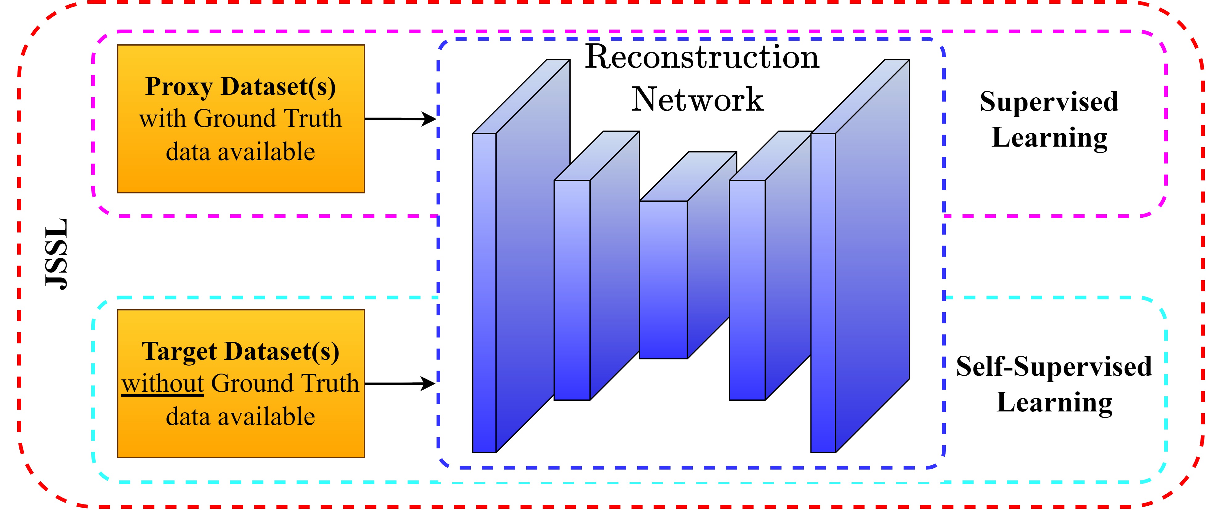
Figure 1: Overview of the Joint Supervised and Self-supervised Learning (JSSL) approach for MRI reconstruction of target datasets without ground truth data. The model is trained using fully sampled (ground truth) data from proxy domain(s) and subsampled data (no ground truth available) from a target domain, in supervised and self-supervised manners, respectively.

In the past half decade, numerous state-of-the-art MRI reconstruction techniques have emerged that employ Deep Learning (DL)-based reconstruction algorithms [3, 14]. These algorithms are trained to produce high-quality images from subsampled $k$-space measurements, surpassing conventional reconstruction methods such as Parallel Imaging [15, 4] or compressed sensing [1, 11]. Typically, these algorithms are trained in a fully supervised manner using retrospectively subsampled $k$-space measurements (or images) as inputs and fully sampled $k$-space data (or images) as ground truth.

Despite the high performance of these methods, there are certain cases in clinical settings where acquiring fully sampled datasets, essential for supervised training, can be infeasible or prohibitively expensive [24, 18, 7]. Such cases include MR imaging of the abdomen, cardiac cine, chest, or the prostate, where periodic or aperiodic motion can make it impossible to collect measurements adhering to the Nyquist-Shannon sampling theorem.

In recent years, to overcome this challenge, several approaches have been proposed that train DL-based algorithms under self-supervised settings, using the available (subsampled) $k$-space measurements without the need for ground truth fully sampled data [25, 13, 31, 2, 6]. These methods harness self-supervised mechanisms to train models to reconstruct subsampled MRI data.

In this work, we introduce Joint Supervised and Self-supervised Learning (JSSL), a novel method for training DL-based MRI reconstruction models when ground truth fully sampled $k$-space data for a target organ domain is unavailable for supervised training. JSSL leverages accessible fully sampled data from proxy dataset(s) and subsampled data from the target dataset(s) to jointly train a model in both supervised and self-supervised manners.

Our contributions can be summarized as follows:

• At the time of writing, our proposed JSSL method represents the first approach to combine supervised and self-supervised learning training within a single pipeline in the context of Accelerated Deep MRI Reconstruction.

• We experimentally demonstrate that JSSL achieves state-of-the-art performance when compared to self-supervised DL-based MRI reconstruction approaches, with a specific focus on a subsampled prostate dataset.

• We provide a theoretical motivation for our approach.

• We offer practical “rule-of-thumb” guidelines for selecting appropriate training frameworks for accelerated MRI reconstruction models.

2 Background and Related Work

2.1 MRI Acquisition and Reconstruction

In Parallel Imaging, assuming a fully sampled MRI acquisition, the ground truth image $\mathbf{x}\in\mathbb{C}^{n}$ can be recovered from the fully sampled multi-coil $k$-space $\mathbf{y}\in\mathbb{C}^{n\times n_{c}}$ by applying the inverse Fourier transform followed by the root-sum-of-squares (RSS) method:

$$\mathbf{x}=\text{RSS}\circ\mathcal{F}^{-1}(\mathbf{y})=\left(\sum_{k=1}^{n_{c}}|\mathcal{F}^{-1}(\mathbf{y}^{k})|^{2}\right)^{1/2}$$ (1)

Alternatively, with known sensitivity maps $\mathbf{S}$, the SENSE method can be applied:

$$\mathbf{x}=\sum_{k=1}^{n_{c}}{\mathbf{S}^{k}}^{*}\mathcal{F}^{-1}(\mathbf{y}^{k}).$$ (2)

In accelerated acquisitions, the fully sampled $k$-space is subsampled via an operator $\mathbf{U}_{\mathbf{M}}$, which selectively retains pixels present in the sampling set $\mathbf{M}$ and sets others to zero:

$$\mathbf{U}_{\mathbf{M}}(\mathbf{y})_{j}=\mathbf{y}_{j}\cdot\mathbb{1}_{\mathbf{M}}(j)=\Bigg{\{}\begin{array}[]{lr}\mathbf{y}_{j},&\text{if }j\in\mathbf{M}\\ 0,&\text{if }j\notin\mathbf{M}.\end{array}$$ (3)

The forward problem of the accelerated acquisition is described by:

$$\tilde{\mathbf{y}}_{\mathbf{M}}=\mathcal{A}_{\mathbf{M},\mathbf{S}}(\mathbf{x})+\mathbf{e},$$ (4)

where $\mathbf{e}\in\mathbb{C}^{n\times n_{c}}$ represents additive measurement noise and $\mathcal{A}_{\mathbf{M},\mathbf{S}}:\mathbb{C}^{n}\rightarrow\mathbb{C}^{n\times n_{c}}$ denotes the forward operator which maps the image $\mathbf{x}\in\mathbb{C}^{n}$ to individual coil images using the coil sensitivity maps $\mathbf{S}$ through the expand operator $\mathcal{E}_{\mathbf{S}}$, applies the two-dimensional fast Fourier transform (FFT), denoted by $\mathcal{F}$, and subsamples them using the subsampling operator $\mathbf{U}_{\mathbf{M}}$:

$$\mathcal{A}_{\mathbf{M},\mathbf{S}}(\mathbf{x})=\mathbf{U}_{\mathbf{M}}\circ\mathcal{F}\circ\mathcal{E}_{\mathbf{S}}(\mathbf{x})=\Big{\{}\mathbf{U}_{\mathbf{M}}\circ\mathcal{F}(\mathbf{S}^{k}\mathbf{x})\Big{\}}_{k=1}^{n_{c}}.$$ (5)

The backward or adjoint operator of $\mathcal{A}_{\mathbf{M},\mathbf{S}}$, denoted by $\mathcal{A}^{*}_{\mathbf{M},\mathbf{S}}:\mathbb{C}^{n\times n_{c}}\rightarrow\mathbb{C}^{n}$, subsamples the input multi-coil data via $\mathbf{U}_{\mathbf{M}}$, maps them to the image domain using the inverse FFT, denoted by $\mathcal{F}^{-1}$, and reduces them to a single image using $\mathbf{S}$ via the reduce operator $\mathcal{R}_{\mathbf{S}}$:

$$\mathcal{A}^{*}_{\mathbf{M},\mathbf{S}}(\mathbf{y})=\mathcal{R}_{\mathbf{S}}\circ\mathcal{F}^{-1}\circ\mathbf{U}_{\mathbf{M}}(\mathbf{y})=\sum_{k=1}^{n_{c}}{\mathbf{S}^{k}}^{*}\mathcal{F}^{-1}\left(\mathbf{U}_{\mathbf{M}}(\mathbf{y}^{k})\right).$$ (6)

2.2 MRI Reconstruction

Typically, the process of recovering an image from the subsampled $k$-space measurements $\tilde{\mathbf{y}}_{\mathbf{M}}$ is formulated as a regularized least squares optimization problem:

$$\mathbf{x}^{*}=\arg\min_{\mathbf{x}^{{}^{\prime}}}\frac{1}{2}\left|\left|\mathcal{A}_{\mathbf{M},\mathbf{S}}(\mathbf{x}^{{}^{\prime}})-\tilde{\mathbf{y}}_{\mathbf{M}}\right|\right|_{2}^{2}+\mathcal{G}(\mathbf{x}^{{}^{\prime}}),$$ (7)

where $\mathcal{G}:\mathbb{C}^{n}\rightarrow\mathbb{R}$ represents an arbitrary regularization functional that incorporates prior reconstruction information. Equation 7 lacks a closed-form solution, and a solution can only be obtained numerically.

2.2.1 Deep Learning based MRI Reconstruction

To circumvent the need for numerical optimization, deep learning methods have been deployed, enabling models to learn the reconstruction process directly from data. A multitude of DL approaches with varying configurations concerning the domain of operation, architectural design, and physics-based considerations have been developed [10, 20].

2.3 MRI Reconstruction with Supervised Learning

In supervised learning (SL) settings, fully sampled $k$-space datasets are assumed to be available. Let $\mathcal{D}^{\text{SL}}=\left\{\mathbf{y}^{(i)}\right\}_{i=1}^{N}$ represent such a dataset, which is retrospectively subsampled during training: $\tilde{\mathbf{y}}_{\mathbf{M}_{i}}^{(i)}=\mathbf{U}_{\mathbf{M}_{i}}(\mathbf{y}^{(i)})$, and let $f_{\bm{\psi}}$ denote a DL-based reconstruction network with trainable parameters $\bm{\psi}$. Note that the architecture of $f_{\bm{\psi}}$ can be configured to output image reconstructions, $k$-space data, or both, but here we assume that both input and output lie in the image domain.

Throughout the paper, we use the notation $\tilde{\cdot}$ for subsampled measurements and $\hat{\cdot}$ for model predictions. The objective in SL-based MRI reconstruction is to minimize the discrepancy between the predicted $k$-space and the fully sampled $k$-space:

$$\begin{gathered}\bm{\psi}^{*}=\arg\min_{\bm{\psi}}\frac{1}{N}\sum_{i=1}^{N}\mathcal{L}_{k}\left(\mathbf{y}^{(i)},\hat{\mathbf{y}}^{(i)}\right)\\ \hat{\mathbf{y}}^{(i)}=\text{DC}_{\mathbf{M}_{i}}\left(\tilde{\mathbf{y}}_{\mathbf{M}_{i}}^{(i)},\hat{\mathbf{y}}_{\mathbf{M}_{i}}^{(i)}\right),\\ \hat{\mathbf{y}}_{\mathbf{M}_{i}}^{(i)}=\mathcal{F}\circ\mathcal{E}_{\mathbf{S}}\circ f_{\bm{\psi}}\left(\tilde{\vec{x}}_{\mathbf{M}_{i}}^{(i)}\right),\,\tilde{\vec{x}}_{\mathbf{M}_{i}}^{(i)}=\mathcal{A}^{*}_{\mathbf{M}_{i},\mathbf{S}}\big{(}\mathbf{y}^{(i)}\big{)},\end{gathered}$$ (8)

or the discrepancy between the predicted image and the reconstructed fully sampled (ground truth) image:

$$\begin{gathered}\bm{\psi}^{*}=\arg\min_{\bm{\psi}}\frac{1}{N}\sum_{i=1}^{N}\mathcal{L}_{\text{I}}\left(\mathbf{x}^{(i)},\hat{\mathbf{x}}^{(i)}\right),\\ \mathbf{x}^{(i)}=\text{RSS}\circ\mathcal{F}^{-1}\left(\mathbf{y}^{(i)}\right),\quad\hat{\mathbf{x}}^{(i)}=\left|f_{\bm{\psi}}\big{(}\tilde{\vec{x}}_{\mathbf{M}_{i}}^{(i)}\big{)}\right|,\end{gathered}$$ (9)

where $\mathcal{L}_{k}$ and $\mathcal{L}_{\text{I}}$ denote arbitrary loss functions computed in the $k$-space and image domains, respectively. The operator DC_M denotes the data consistency operator, which enforces consistency between the available and predicted measurements and is defined as:

$$\text{DC}_{\mathbf{M}}(\mathbf{w}_{1},\,\mathbf{w}_{2})=\mathbf{U}_{\mathbf{M}}(\mathbf{w}_{1})+\mathbf{U}_{\mathbf{M}^{c}}(\mathbf{w}_{2}).$$ (10)

For unseen data $\tilde{\mathbf{y}}^{\text{inf}}_{\mathbf{M}}$ a prediction is estimated as:

$$\hat{\mathbf{x}}=\left|f_{\bm{\psi}^{*}}\big{(}\tilde{\mathbf{x}}^{\text{inf}}_{\mathbf{M}}\big{)}\right|,\quad\tilde{\mathbf{x}}^{\text{inf}}_{\mathbf{M}}=\mathcal{R}_{\mathbf{S}}\circ\mathcal{F}^{-1}\left(\tilde{\mathbf{y}}^{\text{inf}}_{\mathbf{M}}\right).$$ (11)

2.4 SSL-Based Deep MRI Reconstruction

In situations where fully sampled $k$-space data is not available, deep learning models can still be trained using self-supervised learning (SSL). Let $\mathcal{D}^{\text{SSL}}=\big{\{}\tilde{\mathbf{y}}_{\mathbf{M}_{i}}^{(i)}\big{\}}_{i=1}^{N}$ be a dataset containing subsampled acquisitions with each instance $\tilde{\mathbf{y}}_{\mathbf{M}_{i}}^{(i)}$ being sampled in a set $\mathbf{M}_{i}$. To train a reconstruction network under SSL settings, the acquired subsampled measurements are partitioned. Specifically, for each sample $\tilde{\mathbf{y}}_{\mathbf{M}{i}}^{(i)}$, partitioning is performed by splitting the sampling set $\mathbf{M}_{i}$ into two disjoint subsets:

$$\mathbf{\Theta}_{i}\cup\mathbf{\Lambda}_{i}=\mathbf{M}_{i},\quad\mathbf{\Theta}_{i}\cap\mathbf{\Lambda}_{i}=\emptyset,$$ (12)

and then projecting $\tilde{\mathbf{y}}_{\mathbf{M}_{i}}^{(i)}$ onto both subsets, $\mathbf{\Theta}_{i}$ and $\mathbf{\Lambda}_{i}$:

$$\tilde{\mathbf{y}}_{\mathbf{\Theta}_{i}}^{(i)}=\mathbf{U}_{\mathbf{\Theta}_{i}}(\tilde{\mathbf{y}}_{\mathbf{M}_{i}}^{(i)}),\quad\tilde{\mathbf{y}}_{\mathbf{\Lambda}_{i}}^{(i)}=\mathbf{U}_{\mathbf{\Lambda}_{i}}(\tilde{\mathbf{y}}_{\mathbf{M}_{i}}^{(i)}).$$ (13)

Subsequently, one partition is used as input to the reconstruction network, while the other serves as the target. Therefore, the objective loss function is formulated in the $k$-space domain as follows:

$$\begin{gathered}\bm{\psi}^{*}=\arg\min_{\bm{\psi}}\frac{1}{N}\sum_{i=1}^{N}\mathcal{L}_{\textit{k}}\Bigg{(}\tilde{\mathbf{y}}_{\mathbf{\Theta}_{i}}^{(i)},\hat{\mathbf{y}}_{\mathbf{\Theta}_{i}\mathbf{\Lambda}_{i}}^{(i)}\Bigg{)},\\ \hat{\mathbf{y}}_{\mathbf{\Theta}_{i}\mathbf{\Lambda}_{i}}^{(i)}=\mathbf{U}_{\mathbf{\Theta}_{i}}\left(\text{DC}_{\bm{\Lambda}_{i}}\Big{(}\tilde{\mathbf{y}}_{\mathbf{\Lambda}_{i}}^{(i)},\hat{\vec{y}}_{\mathbf{\Lambda}_{i}}^{(i)}\Big{)}\right)\\ \hat{\vec{y}}_{\mathbf{\Lambda}_{i}}^{(i)}=\mathcal{F}\circ\mathcal{E}_{\mathbf{S}}\circ f_{\bm{\psi}}(\tilde{\vec{x}}_{\mathbf{\Lambda}_{i}}^{(i)}),\quad\tilde{\vec{x}}_{\mathbf{\Lambda}_{i}}^{(i)}=\mathcal{A}^{*}_{\mathbf{\Lambda}_{i},\mathbf{S}}\big{(}\tilde{\mathbf{y}}_{\mathbf{M}_{i}}^{(i)}\big{)}.\end{gathered}$$ (14)

The loss can be computed in the image domain as follows:

$$\begin{gathered}\bm{\psi}^{*}=\arg\min_{\bm{\psi}}\frac{1}{N}\sum_{i=1}^{N}\mathcal{L}_{\text{I}}\left(\tilde{\vec{x}}_{\mathbf{\Theta}_{i}}^{(i)},\hat{\mathbf{x}}^{(i)}\right),\\ \tilde{\vec{x}}_{\mathbf{\Theta}_{i}}^{(i)}=\text{RSS}\circ\mathcal{F}^{-1}\left(\tilde{\mathbf{y}}_{\mathbf{\Theta}_{i}}^{(i)}\right),\hat{\mathbf{x}}^{(i)}=\left|\mathcal{R}_{\mathbf{S}}\circ\mathcal{F}^{-1}\left(\hat{\mathbf{y}}_{\mathbf{\Theta}_{i}\mathbf{\Lambda}_{i}}^{(i)}\right)\right|.\end{gathered}$$ (15)

For unseen data $\tilde{\mathbf{y}}^{\text{inf}}_{\mathbf{M}}$ in SSL settings, a prediction is estimated as outlined below:

$$\begin{gathered}\hat{\mathbf{x}}=\left|\mathcal{R}_{\mathbf{S}}\circ\mathcal{F}^{-1}\circ\text{DC}_{\mathbf{M}}\left(\tilde{\mathbf{y}}^{\text{inf}}_{\mathbf{M}},\hat{\mathbf{y}}^{\text{inf}}_{\mathbf{M}}\right)\right|,\\ \hat{\mathbf{y}}^{\text{inf}}_{\mathbf{M}}=\mathcal{F}\circ\mathcal{E}_{\mathbf{S}}\circ f_{\bm{\psi}^{*}}\big{(}\tilde{\mathbf{x}}^{\text{inf}}_{\mathbf{M}}\big{)},\quad\tilde{\mathbf{x}}^{\text{inf}}_{\mathbf{M}}=\mathcal{R}_{\mathbf{S}}\circ\mathcal{F}^{-1}\left(\tilde{\mathbf{y}}^{\text{inf}}_{\mathbf{M}}\right).\end{gathered}$$ (16)

3 Methods

3.1 Joint Supervised and Self-supervised Learning

In this section, we present the Joint Supervised and Self-supervised Learning (JSSL) method. JSSL is a novel approach designed to train DL-based MRI reconstruction models in scenarios where reference data is unavailable in the target organ domain. JSSL combines elements of both supervised and self-supervised learning, employing self-supervised learning using subsampled measurements from the target domain(s) (target dataset(s)) and supervised learning with one or more datasets containing fully sampled acquisitions from other organ domains (proxy datasets). The rationale behind JSSL is to harness the knowledge transferred from the proxy datasets, potentially improving upon conventional self-supervised methods that rely solely on the (subsampled) target dataset(s) for learning. Figure 2 illustrates the end-to-end JSSL pipeline.

3.2 JSSL Training Framework

To implement JSSL, we decompose the overall loss function into two components: one for supervised learning (SL) and another for self-supervised learning (SSL). For simplicity we assume a single target and a single proxy dataset.

Supervised Learning (SL) Loss:

The SL loss is calculated on the proxy dataset, which contains fully sampled $k$-space data. It is formulated as follows:

$$\begin{gathered}{\mathcal{L}}_{\bm{\psi}}^{\text{SL}}={\mathcal{L}_{\text{I}}}_{\bm{\psi}}^{\text{SL}}+{\mathcal{L}_{k}}_{\bm{\psi}}^{\text{SL}}\\ {\mathcal{L}_{\text{I}}}_{\bm{\psi}}^{\text{SL}}=\frac{1}{N_{\text{prx}}}\sum_{i=1}^{N_{\text{prx}}}\mathcal{L}_{\text{I}}\left(\mathbf{x}^{\text{prx},(i)},\hat{\mathbf{x}}^{\text{prx},(i)}\right),\\ {\mathcal{L}_{k}}_{\bm{\psi}}^{\text{SL}}=\frac{1}{N_{\text{prx}}}\sum_{i=1}^{N_{\text{prx}}}\mathcal{L}_{k}\left(\mathbf{y}^{\text{prx},(i)},\hat{\mathbf{y}}^{\text{prx},(i)}\right).\end{gathered}$$ (17)

Here, $\mathbf{x}^{\text{prx},(i)}$ , $\hat{\mathbf{x}}^{\text{prx},(i)}$ represent the ground truth and predicted images, respectively, for the $i$-th sample in the proxy dataset, while $\mathbf{y}^{\text{prx},(i)}$, $\hat{\mathbf{y}}^{\text{prx},(i)}$ represent the fully sampled and predicted $k$-spaces, respectively, as defined in Section 2.3.

Self-supervised Learning (SSL) Loss:

The SSL loss is calculated using the target dataset, which consists of subsampled $k$-space data without ground truth. In contrast to many SSL-based methods, we calculate the SSL loss in both the image and $k$-space domains as follows:

$$\begin{gathered}{\mathcal{L}}_{\bm{\psi}}^{\text{SSL}}={\mathcal{L}_{\text{I}}}_{\bm{\psi}}^{\text{SSL}}+{\mathcal{L}_{k}}_{\bm{\psi}}^{\text{SSL}}\\ {\mathcal{L}_{k}}_{\bm{\psi}}^{\text{SSL}}=\frac{1}{N_{\text{tar}}}\sum_{i=1}^{N_{\text{tar}}}\mathcal{L}_{k}\left(\tilde{\mathbf{y}}_{\mathbf{\Theta}_{i}}^{\text{tar},(i)},\hat{\mathbf{y}}_{\mathbf{\Theta}_{i}\mathbf{\Lambda}_{i}}^{\text{tar},(i)}\right),\\ {\mathcal{L}_{\text{I}}}_{\bm{\psi}}^{\text{SSL}}=\frac{1}{N_{\text{tar}}}\sum_{i=1}^{N_{\text{tar}}}\mathcal{L}_{\text{I}}\left(\tilde{\vec{x}}_{\mathbf{\Theta}_{i}}^{\text{tar},(i)},\hat{\mathbf{x}}^{\text{tar},(i)}\right),\\ \tilde{\vec{x}}_{\mathbf{\Theta}_{i}}^{\text{tar},(i)}=\text{RSS}\circ\mathcal{F}^{-1}(\tilde{\mathbf{y}}_{\mathbf{\Theta}_{i}}^{\text{tar},(i)}),\quad\hat{\mathbf{x}}^{\text{tar},(i)}=\left|f_{\bm{\psi}}(\tilde{\vec{x}}_{\mathbf{\Lambda}_{i}}^{\text{tar},(i)})\right|,\end{gathered}$$ (18)

where, $\tilde{\vec{x}}_{\mathbf{\Lambda}_{i}}^{\text{tar},(i)}$, $\tilde{\mathbf{y}}_{\mathbf{\Theta}_{i}}^{\text{tar},(i)}$, $\hat{\mathbf{y}}_{\mathbf{\Theta}_{i}\mathbf{\Lambda}_{i}}^{\text{tar},(i)}$ are as defined in Section 2.4.

JSSL Loss:

The JSSL loss is a fundamental component of our approach, defined as the sum of the SL and SSL losses:

$$\mathcal{L}_{\bm{\psi}}^{\text{JSSL}}={\mathcal{L}}_{\bm{\psi}}^{\text{SL}}+{\mathcal{L}}_{\bm{\psi}}^{\text{SSL}}.$$ (19)

The model’s parameters are updated during training to minimize the JSSL loss:

$$\bm{\psi}^{*}=\arg\min_{\bm{\psi}}\mathcal{L}_{\bm{\psi}}^{\text{JSSL}}.$$ (20)

3.3 JSSL at Inference

During the inference phase, the trained JSSL reconstruction model $f_{\bm{\psi}^{*}}$ estimates the underlying image as follows:

$$\hat{\mathbf{x}}=\left|f_{\bm{\psi}^{*}}\big{(}\tilde{\mathbf{x}}^{\text{inf}}_{\mathbf{M}}\big{)}\right|,\quad\tilde{\mathbf{x}}^{\text{inf}}_{\mathbf{M}}=\mathcal{R}_{\mathbf{S}}\circ\mathcal{F}^{-1}\left(\tilde{\mathbf{y}}^{\text{inf}}_{\mathbf{M}}\right),$$ (21)

where $\tilde{\mathbf{y}}^{\text{inf}}_{\mathbf{M}}$ denotes the subsampled $k$-space data.

3.4 JSSL: A Theoretical Motivation

In this section, we offer a theoretical motivation for JSSL. The core concept behind JSSL is to leverage both supervised and self-supervised learning to enhance MRI reconstruction of a target dataset, even when the parameters optimized on supervised proxy tasks may not be the most optimal. We hypothesize that introducing a supervised proxy task serves as a form of regularization, reducing the variance of our estimators due to the proxy supervised training on ‘less noisy’ task. We illustrate this intuition with two simplified examples in Propositions 1 (estimating means of distributions) and 2 (linear regression), where we assume two distributions - one that we wish to estimate, but we cannot obtain sufficient samples from, and a proxy distribution that is directly accessible. We demonstrate that drawing samples from both distributions (or using only the proxy distribution) can reduce our estimator’s variance and risk.

Proposition 1.

Consider two distributions $p_{i},\,i=1,2$ with means and variances ${\mu}_{i},{\sigma}_{i},\,i=1,2$, with unknown ${\mu}_{1}$, and ${\mu}_{1}\neq{\mu}_{2}$. Then if $(\mu_{1}-\mu_{2})^{2}<c\frac{{\sigma}_{1}^{2}}{N}$ for some $c\in(0,1)$ and $N\in\mathbb{Z}^{+}$, then $\tilde{{x}}=\frac{1}{N+K}\sum_{i=1}^{N+K}{x}_{i}$ is a lower-variance estimator of $\mu_{1}$ compared to $\overline{{x}}=\frac{1}{N}\sum_{i=1}^{N}{x}_{i}$, where $\left\{{x}^{(i)}\sim p_{1}\right\}_{i=1}^{N}$ and $\left\{{x}^{(N+i)}\sim p_{2}\right\}_{i=1}^{K}$ for a choice of a large $K\in\mathbb{Z}^{+}$.

Proof.

See Supplementary Material A. ∎

Proposition 2.

Let $\bm{x}\sim\mathcal{N}(\bm{0},\sigma^{2}\bm{I}_{p})$ be $\mathbb{R}^{p}$-valued isotropic Gaussian random vector and $y,\tilde{y}$ be random variables with $p(y|\bm{x})=\mathcal{N}(y|\bm{w}^{T}\bm{x},\varepsilon^{2})$ and $p(\tilde{y}|\bm{x})=\mathcal{N}(\tilde{y}|\bm{\tilde{w}}^{T}\bm{x},\tilde{\varepsilon}^{2})$ for some $\bm{w},\bm{\tilde{w}}\in\mathbb{R}^{p}$. Let $\mathcal{T}=\{(\bm{x}_{1},\tilde{y}_{1}),\dots,(\bm{x}_{K},\tilde{y}_{K})\}$ be a training data set with $K>p$ and consider a maximum likelihood estimator $\widehat{y}(\bm{x};\mathcal{T})$. Then the following holds:

1. $\mathrm{Bias}_{\mathcal{T}}[\widehat{y}(\bm{x};\mathcal{T})]=(\bm{\tilde{w}}^{T}-\bm{w}^{T})\bm{x}.$

2. $\mathrm{Var}_{\mathcal{T}}[\widehat{y}(\bm{x};\mathcal{T})]=\frac{\tilde{\varepsilon}^{2}}{\sigma^{2}K}\|\bm{x}\|_{2}^{2}$.

3. $\mathbb{E}_{(\bm{x},y)}[\widehat{y}(\bm{x};\mathcal{T})-y]^{2}\leq p\sigma^{2}\|\bm{\tilde{w}}-\bm{w}\|_{2}^{2}+\frac{p\tilde{\varepsilon}^{2}}{K}+\varepsilon^{2}$

Proof.

See Supplementary Material A. ∎

Propositions 1 and 2 imply that drawing many samples from the proxy distribution ($K\to\infty$), can result in a lower variance of our estimator trained under SL and SSL settings.

Figure 2: (a) The training process for the proposed Joint Supervised and Self-supervised Learning (JSSL) method is divided into two phases: (1) Supervised Learning (SL) using fully sampled $k$-space data from proxy datasets. During this phase, the model is trained to predict fully sampled data from retrospectively subsampled proxy data. (2) Self-supervised Learning (SSL) utilizing subsampled $k$-space data from the target dataset, partitioned into two disjoint subsets. The model takes one subset as input and aims to predict the other. Loss functions are defined for both SL and SSL settings in both $k$-space and image domains and the JSSL loss comprises all these components. The model is jointly trained with both supervised and self-supervised loss functions to enhance MRI reconstruction in the target domain. In all phases, sensitivity maps $\mathbf{S}$ are learned using the autocalibration signal (center of $k$-space) from available measurements. A U-Net, functioning as a SME module, is trained end-to-end with the reconstruction network (omitted in the diagram). (b) In the inference phase, the trained network predicts the underlying ground truth image from the target dataset based on input subsampled data.

3.5 Reconstruction Network

Unrolled DL-based MRI reconstruction methods have demonstrated significant reconstruction capabilities in both supervised and self-supervised approaches [25, 9, 5, 28]. In this study, for our experiments, we employed the variable Splitting Half-quadratic Admm algorithm for Reconstruction of inverse-Problems (vSHARP) as our reconstruction network, which is an unrolled physics-guided DL-based method [27] that has previously been applied in accelerated prostate and dynamic cardiac MRI reconstruction [27, 26].

The vSHARP algorithm incorporates the half-quadratic variable splitting method to the optimization problem presented in (7), introducing an auxiliary variable $\mathbf{z}$:

$$\min_{\mathbf{x}^{{}^{\prime}},\mathbf{z}}\frac{1}{2}\left|\left|\mathcal{A}_{\mathbf{M},\mathbf{S}}(\mathbf{x}^{{}^{\prime}})-\tilde{\mathbf{y}}_{\mathbf{M}}\right|\right|_{2}^{2}+\mathcal{G}(\mathbf{z})\quad\text{s.t. }\mathbf{x}^{{}^{\prime}}=\mathbf{z}.$$ (22)

Subsequently, (22) is iteratively unrolled over $T$ iterations using the Alternating Direction Method of Multipliers (ADMM). The ADMM formulation consists of three key steps: (a) a denoising step to refine the auxiliary variable $\mathbf{z}$, (b) data consistency for the target image $\mathbf{x}$, and (c) an update for the Lagrange Multipliers $\mathbf{u}$ introduced by ADMM:

$$\mathbf{z}_{t+1}=\mathcal{H}_{\bm{\psi}_{t+1}}\left(\mathbf{z}_{t},\mathbf{x}_{t},\mathbf{u}_{t}/{\mu}_{t+1}\right),$$ (23a)

$$\mathbf{x}_{t+1}=\arg\min_{\mathbf{x}^{{}^{\prime}}}\Big{|}\Big{|}\mathcal{A}_{\mathbf{M},\mathbf{S}}(\mathbf{x}^{{}^{\prime}})\,-\,\tilde{\mathbf{y}}_{\mathbf{M}}\Big{|}\Big{|}_{2}^{2}+\mu\left|\left|\mathbf{x}^{{}^{\prime}}-\mathbf{z}_{t+1}+\mathbf{u}_{t}/{\mu}_{t+1}\right|\right|_{2}^{2},$$ (23b)

$$\mathbf{u}_{t+1}=\mathbf{u}_{t}+\mu_{t+1}\left(\mathbf{x}_{t+1}-\mathbf{z}_{t+1}\right).$$ (23c)

In (23a), $\mathcal{H}_{\bm{\psi}_{t+1}}$ denotes a convolutional based DL image denoiser with trainable parameters $\bm{\psi}_{t+1}$, and $\eta_{t+1}$ a trainable learning rate. At each iteration, $\mathcal{H}_{\bm{\psi}_{t+1}}$ takes as input the previous predictions of the three variables and outputs an estimation of the auxiliary variable $\mathbf{z}$. Equation 23b is solved numerically by unrolling further a gradient descent scheme over $T_{\mathbf{x}}$ iterations. The last step in (23c), involves a straightforward computation.

The initial approximations for $\mathbf{x}$ and $\mathbf{z}$ are taken as:

$$\mathbf{x}_{0},\,\mathbf{z}_{0}=\mathcal{R}_{\mathbf{S}}\circ\mathcal{F}^{-1}\left(\tilde{\mathbf{y}}_{\mathbf{M}}\right).$$ (24)

Additionally, for $\mathbf{u}_{0}$, vSHARP employs a trainable replication-padding and dilated convolutional-based network represented by $\mathcal{U}_{\bm{\phi}}$ with trainable parameters $\bm{\phi}$:

$$\mathbf{u}_{0}=\mathcal{U}_{\bm{\phi}}(\mathbf{x}_{0}).$$ (25)

3.6 Coil Sensitivity Prediction

The initial approximation of coil sensitivity maps is derived from the autocalibration signal, specifically the center of the $k$-space[12]. While SSL-based approaches such as [25, 31] use this initial approximation or employ computationally expensive and time-consuming algorithms like ESPIRiT [23] to refine it, our JSSL approach takes this initial estimation and feeds it as input to a Sensitivity Map Estimator (SME). The SME is a DL-based model designed to enhance and refine the sensitivity profiles and it is trained end-to-end in conjunction with the reconstruction model. Note that we integrate an identical SME module in our SSL-based experiments.

4 Experiments

4.1 Datasets

To assess the performance of JSSL, we conducted experiments using two proxy datasets and one target dataset:

Proxy Datasets As proxy datasets, we utilized the brain fastMRI and knee fastMRI datasets [30]. The brain MRI dataset comprises fully sampled $k$-space brain volumes, including axial T1 and T2-weighted, and FLAIR images. The knee MRI dataset consists of fully sampled knee $k$-space data and contains coronal proton density-weighted images with and without fat suppression. Both datasets feature multi-coil acquisitions. It is worth noting that the number of coils in the brain dataset ranges from 2 to 28, while the knee dataset was acquired using 16 coils. We utilized 29,991 volumes (47,426 slices) and 973 volumes (34,742 slices) from the train brain and knee, respectively, datasets. During training, data were retrospectively subsampled, while fully sampled measurements were used for loss calculation.

Target Dataset As target dataset, we employed the prostate fastMRI dataset [22]. This dataset includes fully sampled multi-coil $k$-space data from 312 subjects for T2-weighted acquisitions. The coil configurations for this dataset varied from 10 to 30 coils. To create training, validation, and testing sets, we divided the subjects into 218 (6,647 slices), 48 (1,462 slices), and 46 (1,399 slices) volumes, respectively. During training, fully sampled data from the dataset were retrospectively subsampled, and we only used the fully sampled data for evaluation at inference. Given the substantial difference in the number of training samples between the proxy and target datasets, we employed a double oversampling strategy on the training prostate data.

4.2 Subsampling Schemes

For our experiments, we used a random uniform Cartesian subsampling scheme for the brain and an equispaced Cartesian subsampling scheme for the knee measurements, following the corresponding publication [30]. Similarly, for the target prostate data, we enforced an equispaced subsampling scheme as it’s one of the easiest and fastest to implement on MRI machines, suitable for prostate imaging.

The subsampling process during training involved selecting acceleration factors of $R=$ 4, 8, or 16. Specifically, for an acceleration factor of 4, 8% of the fully sampled data were retained as autocalibration signal (ACS) lines (center of $k$-space). Similarly, for acceleration factors of 8 and 16, the corresponding percentages of ACS lines were 4% and 2% of the fully sampled data, respectively, as described in [29]. During inference, our methods were tested under acceleration factors of $R=$ 2, 4, 8, and 16, with ACS percentages of 16%, 8%, 4%, and 2%, respectively.

4.3 SSL Subsampling Partitioning

During the training of any SSL-based method, including JSSL, in our experiments, the subsampled data underwent partitioning into two distinct sets, as elaborated in Section 2.4. To achieve this, $\mathbf{\Theta}_{i}$ was obtained by selecting elements from ${\mathbf{M}_{i}}$ via a 2D Gaussian scheme with a standard deviation of 3.5 pixels. Consequently, we set ${\mathbf{\Lambda}_{i}}={\mathbf{M}_{i}\setminus\mathbf{\Theta}_{i}}$ (more information is provided in Supplementary Material B). Furthermore, the ratio $q_{i}=\frac{|\mathbf{\Theta}_{i}|}{|\mathbf{M}_{i}|}$ was randomly selected between 0.3 and 0.8. An illustrative example of this is provided in Fig. 3. Note that a $w\times w=4\times 4$ window in the center of the ACS region was included in each $\mathbf{\Lambda}_{i}$ to facilitate effective training of the SME module.

(a) $\mathbf{M}_{i}$

(b) $\mathbf{\Theta}_{i}$

(c) $\mathbf{\Lambda}_{i}=\mathbf{M}_{i}\smallsetminus\mathbf{\Theta}_{i}$

Figure 3: Example of SSL subsampling partitioning with a ratio $q=\frac{1}{2}$ and $w=4$.

4.4 Implementation & Optimization

Model Architecture

In all our experiments, we adopted vSHARP with $T=12$ optimization steps, utilizing two-dimensional U-Nets [17] composed of 4 scales and 32 filters (in the first scale) for $\left\{\mathcal{H}_{\bm{\theta}_{t}}\right\}_{t=0}^{T-1}$. For the data consistency step, we set $T_{\mathbf{x}}=10$. For the SME module we employed a 2D U-Net with 4 scales and 16 filters in the first scale.

Parameter Optimization

We optimized the model parameters using the Adam optimizer [8], with parameters $\epsilon=10^{-8}$, $(\beta_{1},\beta_{2})=(0.99,0.999)$ and initial learning rate (lr) set to 0.003. We also employed a lr scheduler which decayed the lr by a factor of 0.8 every 150,000 training iterations. Our experiments were carried out on two A6000 RTX GPUs, with a batch size of 2 slices of multi-coil $k$-space data assigned to each GPU.

Choice of Loss Function

In all our experiments, loss was computed as detailed in Sec. 3.2 employing the following:

$$\begin{gathered}{\mathcal{L}_{\text{I}}}^{\text{SL}},\,{\mathcal{L}_{\text{I}}}^{\text{SSL}}:=2\left(1-\text{SSIM}+\mathcal{L}_{1}\right)+\text{HFEN}_{1}+\text{HFEN}_{2},\\ {\mathcal{L}_{k}}^{\text{SL}},\,{\mathcal{L}_{k}}^{\text{SSL}}:=2\left(\text{NMSE}+\text{NMAE}\right).\end{gathered}$$ (26)

For brevity, we have omitted the definitions of the individual components of these loss functions. Comprehensive details can be found in the Supplementary Material B.

4.5 Training Setups Comparison

Here, we present the comparisons that were conducted to evaluate JSSL for accelerated MRI reconstruction. All of our experiments were evaluated on the test set of the target prostate dataset, with the aim of assessing the performance of each strategy. We performed the following experiments:

1. SSL in the target domain.

2. SSL in both the target and proxy domains (SSL ALL).

3. SL in the target domain.

4. SL in both the proxy and target domains (SL ALL).

5. JSSL (SL in proxy domain, SSL in target domain).

Our principal objective throughout these comparisons was to examine the performance of JSSL in relation to SSL training approaches, since we are interested in scenarios where there is no access to fully sampled data in the target domain. To demonstrate that JSSL’s superiority does not solely stem from the larger dataset size (more data from the proxy datasets), we also conducted experiments using all available data using and SSL strategy, incorporating both the target and proxy datasets. SL-based experiments served as reference, although naturally, the results are expected to favor SL methods when fully sampled data is accessible in the target domain.

4.6 Ablation Studies

To investigate JSSL further and demonstrate its superiority under different settings, we examine additional configurations for the JSSL and SSL setups. In particular, we perform the following experiments:

1. JSSL and SSL in all domains by oversampling $10\times$ the target dataset during training to balance better proxy and target data, in comparison to $2\times$ in our original experiments in Sec. 4.5.

2. JSSL and SSL using a constant partitioning ratio of $q=0.5$ instead of random $q=0.3-0.8$ as in Sec. 4.5.

3. JSSL and SSL setting for the ACS window $w^{2}=10^{2}$ opposed to $w^{2}=4^{2}$ in our experiments in Sec. 4.5.

In Supplementary Material C, we include further experiments with different reconstruction network choices.

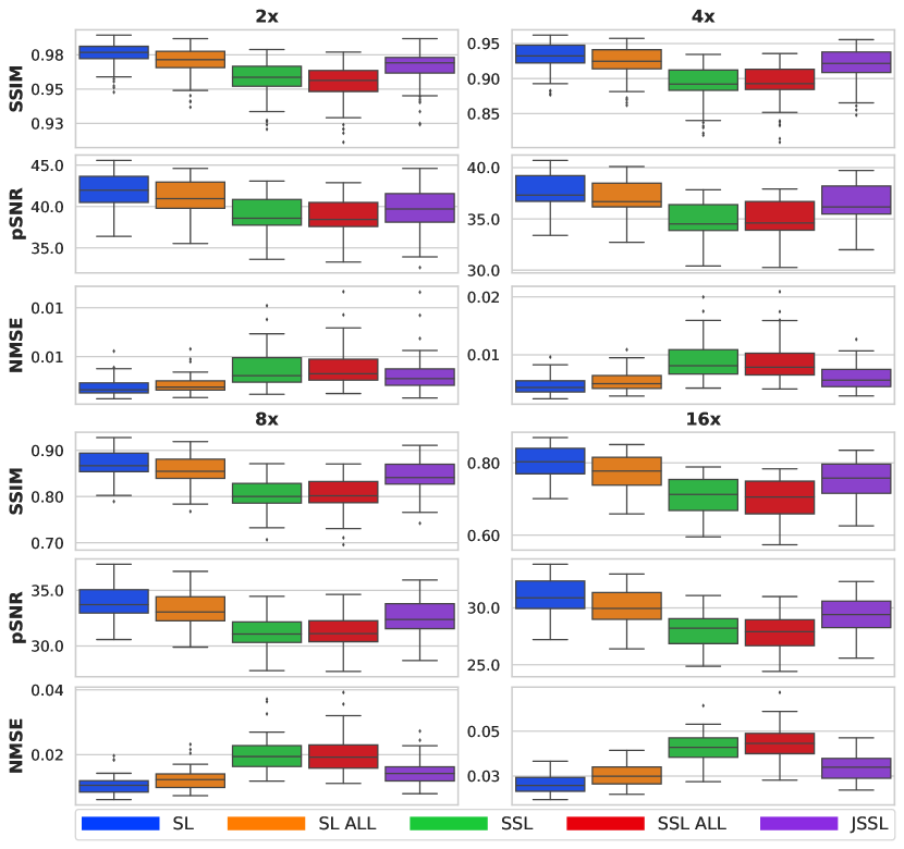
Figure 4: Evaluation results for different training setups.

5 Results & Discussion

5.1 Evaluation

To assess the results of our experiments, we employed three key metrics: the Structural Similarity Index Measure (SSIM), peak Signal-to-Noise Ratio (pSNR), and normalized mean squared error (NMSE). Metrics were calculated by comparing model outputs with the RSS ground truth reconstructions, as detailed in (1). The metric definitions were consistent with [29]. The selection of optimal model checkpoints was based on their performance on the validation set.

5.2 Comparison Results

Table 1: Average metric results across different training setups.

Setup		2x				4x				8x				16x
		SSIM	pSNR	NMSE		SSIM	pSNR	NMSE		SSIM	pSNR	NMSE		SSIM	pSNR	NMSE
SL		0.974	41.8	0.002		0.930	37.5	0.005		0.868	33.9	0.011		0.799	31.0	0.021
SL ALL		0.969	41.1	0.002		0.922	36.9	0.005		0.854	33.2	0.013		0.771	30.0	0.026
SSL		0.956	38.8	0.004		0.891	34.7	0.009		0.801	31.1	0.020		0.707	28.0	0.041
SSL ALL		0.953	38.6	0.004		0.892	34.8	0.009		0.801	31.1	0.020		0.699	27.8	0.043
JSSL		0.965	39.5	0.003		0.918	36.4	0.006		0.842	32.5	0.015		0.752	29.3	0.030

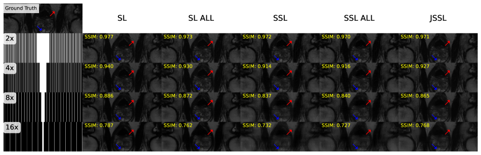
Figure 5: Example reconstructions of a slice subsampled at different acceleration factors (left-most column) from the test set from each training setup. Arrows point to regions of interest.

The results of our comparative studies, as described in Sec. 4.5, are visually represented in Fig. 4 using box plots, while Tab. 1 presents the corresponding metric averages. As anticipated, supervised (SL) tasks demonstrated the highest performance. An intriguing observation emerged when proxy datasets were introduced in the supervised learning setting; the reconstruction performance on the target dataset decreased. This suggests the potential imposition of bias on the trained model’s parameters by the proxy datasets.

Most notably, the Joint Self-supervised Learning (JSSL) setup exhibited superior reconstruction results across all acceleration factors and metrics compared to both SSL and SSL utilizing both proxy and target datasets (SSL ALL). Specifically, for acceleration factors 2, 4, and 8, the JSSL approach proved to be a robust competitor to supervised tasks. In contrast, employing proxy datasets under SSL settings (SSL ALL) did not appear to enhance reconstruction performance, as evident from Fig. 4 and Tab. 1, in line with the supervised experiments.

For visual assessment, in Fig. 5 we illustrate sample image reconstructions across all acceleration factors and training setups. Although for acceleration factors (2 and 4) all methods reconstructed the accelerated data faithfully, for higher accelerations only the supervised and JSSL setups were able to reconstruct the images with less artifacts.

5.3 Ablation Results

Table 2: Average results for ablative settings.

Setup		2x				4x				8x				16x
		SSIM	pSNR	NMSE		SSIM	pSNR	NMSE		SSIM	pSNR	NMSE		SSIM	pSNR	NMSE
SSL Original		0.956	38.8	0.004		0.891	34.7	0.009		0.801	31.1	0.020		0.707	28.0	0.041
SSL ALL Original		0.953	38.6	0.004		0.892	34.8	0.009		0.801	31.1	0.020		0.699	27.8	0.043
JSSL Original		0.965	39.5	0.003		0.918	36.4	0.006		0.842	32.5	0.015		0.752	29.3	0.030
SSL ALL Oversamp.		0.953	38.6	0.004		0.892	34.8	0.009		0.801	31.1	0.020		0.699	27.8	0.043
JSSL Oversamp.		0.968	41.0	0.002		0.919	36.7	0.006		0.842	32.6	0.014		0.749	29.2	0.031
SSL (q=0.5)		0.957	39.1	0.003		0.895	35.0	0.008		0.817	31.7	0.017		0.733	28.9	0.033
SSL ALL (q=0.5)		0.955	38.5	0.004		0.891	34.6	0.009		0.807	31.3	0.019		0.712	28.1	0.040
JSSL (q=0.5)		0.965	39.7	0.003		0.919	36.6	0.006		0.842	32.6	0.014		0.743	29.0	0.032
SSL (w=10)		0.954	38.4	0.004		0.893	34.7	0.009		0.815	31.6	0.018		0.726	28.5	0.036
SSL ALL (w=10)		0.954	38.4	0.004		0.890	34.6	0.009		0.805	31.2	0.020		0.710	28.1	0.040
JSSL (w=10)		0.958	38.7	0.004		0.916	36.4	0.006		0.839	32.5	0.015		0.748	29.2	0.031

Summarized in Tab. 2, we calculated the average evaluation metrics on the test set for our ablation experiments, providing additional context to the JSSL approach. These experiments consistently showcased the superior performance of JSSL over SSL setups, in line with our prior observations. Interestingly, variations in the training hyper-parameters for JSSL, such as oversampling, partitioning ratio ($q=0.5$), and ACS window size ($w=10$), did not yield significant improvements or deteriorations in performance, except for an observable improvement in average pSNR at $R=2$.

Regarding the SSL setups, an observable enhancement was witnessed for 8$\times$ and 16$\times$ accelerated data when adopting a fixed partitioning ratio $q=0.5$ or a larger ACS window of $w^{2}=10^{2}$ pixels. However, this improvement was particularly evident in the SSL setup using solely the (subsampled) proxy dataset. Furthermore, the inclusion of proxy datasets within SSL configurations (SSL ALL) did not yield improvements in reconstruction performance, consistent with our earlier findings in the comparative study.

For further assessment, we provide in Supplementary Material D box plots illustrating comprehensively the performance metrics, as well as sample reconstructions for each setup studied in the ablation study.

6 Conclusion

In conclusion, we have introduced the JSSL approach for training deep-learning accelerated MRI reconstruction models as a superior alternative to self-supervised methods. JSSL effectively utilizes fully sampled data from proxy datasets and subsampled data from target datasets for simultaneous supervised and self-supervised training, respectively. Our comparative and ablation experiments establish the superiority of JSSL over current SSL-based approaches.

Based on our empirical findings, we propose practical training “rule-of-thumb” guidelines when determining the approach for deep MRI reconstruction algorithms:

1. If ground truth data are available for the target dataset, opt for supervised training.

2. If ground truth data are not available for the target dataset but subsampled data are present, and ground truth data exist from other datasets, consider adopting the JSSL approach.

3. In cases where only subsampled data are accessible for the target dataset without ground truth data from other proxy datasets, proceed with self-supervised training. A fixed partitioning ratio might be preferable for high acceleration factors.

Supplementary Material

Appendix A JSSL Theoretical Motivation Proofs

In this appendix we provide the proofs for the theoretical motivations for the JSSL method presented in Section 3.4 of the main paper.

Proposition 1.

Consider two distributions $p_{i},\,i=1,2$ with means and variances ${\mu}_{i},{\sigma}_{i},\,i=1,2$, with unknown ${\mu}_{1}$, and ${\mu}_{1}\neq{\mu}_{2}$. Then if $(\mu_{1}-\mu_{2})^{2}<c\frac{{\sigma}_{1}^{2}}{N}$ for some $c\in(0,1)$ and $N\in\mathbb{Z}^{+}$, then $\tilde{{x}}=\frac{1}{N+K}\sum_{i=1}^{N+K}{x}_{i}$ is a lower-variance estimator of $\mu_{1}$ compared to $\overline{{x}}=\frac{1}{N}\sum_{i=1}^{N}{x}_{i}$, where $\left\{{x}^{(i)}\sim p_{1}\right\}_{i=1}^{N}$ and $\left\{{x}^{(N+i)}\sim p_{2}\right\}_{i=1}^{K}$ for a choice of a large $K\in\mathbb{Z}^{+}$.

Proof.

Assume a mixture distribution:

$$p_{\pi}(x)=\pi\mathcal{N}(x|{\mu}_{1},{\sigma}_{1}^{2})+(1-\pi)\mathcal{N}(x|{\mu}_{2},{\sigma}_{2}^{2}).$$

It is then straightforward to compute:

$$\begin{gathered}\mathbb{E}\left[p_{\pi}\right]=\pi{\mu}_{1}+(1-\pi){\mu}_{2}\end{gathered}$$

and,

$$\mathbb{V}\left[p_{\pi}\right]=\pi{\sigma}_{1}^{2}+(1-\pi){\sigma}_{2}^{2}+\pi(1-\pi)({\mu}_{2}-{\mu}_{1})^{2}.$$

Drawing $\displaystyle\left\{{x}^{(i)}\sim p_{1}\right\}_{i=1}^{N}$ and $\displaystyle\left\{{x}^{(N+i)}\sim p_{2}\right\}_{i=1}^{K}$, is approximately equivalent to drawing $N+K$ samples from the mixture $p_{\pi}$ with $\pi=\frac{N}{N+K}$. Using bias-variance decomposition, we can compute the expected mean squared errors for the two estimators:

$$\mathbb{E}\left[(\overline{{x}}-{\mu}_{1})^{2}\right]=\frac{{\sigma}_{1}^{2}}{N},$$

and,

$$\mathbb{E}\left[(\tilde{{x}}-{\mu}_{1})^{2}\right]=(1-\pi)^{2}(\mu_{1}-\mu_{2})^{2}+\frac{\pi\sigma_{1}^{2}+(1-\pi)\sigma_{2}^{2}+\pi(1-\pi)(\mu_{1}-\mu_{2})^{2}}{N+K}.$$

If $(\mu_{1}-\mu_{2})^{2}<c\frac{{\sigma}_{1}^{2}}{N}$ for some $c\in(0,1)$, then taking the limit $K\to\infty$ and thus $\pi\to 0$, we observe that

$$\mathbb{E}\left[(\tilde{{x}}-{\mu}_{1})^{2}\right]\to(\mu_{1}-\mu_{2})^{2}<c\frac{{\sigma}_{1}^{2}}{N}<\frac{{\sigma}_{1}^{2}}{N}=\mathbb{E}\left[(\overline{{x}}-{\mu}_{1})^{2}\right].$$

∎

Proposition 2.

Let $\bm{x}\sim\mathcal{N}(\bm{0},\sigma^{2}\bm{I}_{p})$ be $\mathbb{R}^{p}$-valued isotropic Gaussian random vector and $y,\tilde{y}$ be random variables with $p(y|\bm{x})=\mathcal{N}(y|\bm{w}^{T}\bm{x},\varepsilon^{2})$ and $p(\tilde{y}|\bm{x})=\mathcal{N}(\tilde{y}|\bm{\tilde{w}}^{T}\bm{x},\tilde{\varepsilon}^{2})$ for some $\bm{w},\bm{\tilde{w}}\in\mathbb{R}^{p}$. Let $\mathcal{T}=\{(\bm{x}_{1},\tilde{y}_{1}),\dots,(\bm{x}_{K},\tilde{y}_{K})\}$ be a training data set with $K>p$ and consider a maximum likelihood estimator $\widehat{y}(\bm{x};\mathcal{T})$ for $y$ given $\bm{x}$, computed using $\mathcal{T}$. Then the following holds:

1. $\mathrm{Bias}_{\mathcal{T}}[\widehat{y}(\bm{x};\mathcal{T})]=(\bm{\tilde{w}}^{T}-\bm{w}^{T})\bm{x}.$

2. $\mathrm{Var}_{\mathcal{T}}[\widehat{y}(\bm{x};\mathcal{T})]=\frac{\tilde{\varepsilon}^{2}}{\sigma^{2}K}\|\bm{x}\|_{2}^{2}$.

3. $\mathbb{E}_{(\bm{x},y)}[\widehat{y}(\bm{x};\mathcal{T})-y]^{2}\leq p\sigma^{2}\|\bm{\tilde{w}}-\bm{w}\|_{2}^{2}+\frac{p\tilde{\varepsilon}^{2}}{K}+\varepsilon^{2}$

Proof.

Let $\bm{\tilde{w}}_{\mathrm{MLE}}=(\bm{X}^{T}\bm{X})^{-1}\bm{X}^{T}\bm{\tilde{y}}$ be the MLE estimator for $\bm{\tilde{w}}$, where the $K$ rows of $\bm{X}\in\mathbb{R}^{K\times p}$ are given by $\bm{x}_{1}^{T},\dots,\bm{x}_{K}^{T}$ and the vector $\bm{\tilde{y}}$ is defined as $\bm{\tilde{y}}:=(\tilde{y}_{1},\dots,\tilde{y}_{K})\in\mathbb{R}^{K}$. Since $K>p$, matrix $\bm{X}$ has full column rank almost surely and thus $\bm{X}^{T}\bm{X}$ is almost surely invertible. Observe that

$$\mathbb{E}_{\mathcal{T}}[\bm{\tilde{w}}_{\mathrm{MLE}}^{T}]=\mathbb{E}_{\mathcal{T}}[(\bm{\tilde{\varepsilon}}^{T}+\bm{\tilde{w}}^{T}\bm{X}^{T})\bm{X}(\bm{X}^{T}\bm{X})^{-1}]=\bm{\tilde{w}}^{T},$$

since $\bm{\tilde{\varepsilon}}:=\bm{\tilde{y}}-\bm{X}\bm{\tilde{w}}$ has zero mean, is independent from $\bm{x}_{i}$’s and the expectation $\mathbb{E}_{\mathcal{T}}[\cdot]$ can be rewritten as $\mathbb{E}_{\bm{x}_{1},\dots,\bm{x}_{K}}[\mathbb{E}_{\bm{\tilde{\varepsilon}}}[\cdot]]$. By definition of estimator bias,

$$\mathrm{Bias}_{\mathcal{T}}[\widehat{y}(\bm{x};\mathcal{T})]=\mathbb{E}_{\mathcal{T}}[\widehat{y}(\bm{x};\mathcal{T})]-\mathbb{E}_{y|\bm{x}}y=\mathbb{E}_{\mathcal{T}}[\bm{\tilde{w}}_{\mathrm{MLE}}^{T}]\bm{x}-\bm{w}^{T}\bm{x}=(\bm{\tilde{w}}^{T}-\bm{w}^{T})\bm{x}.$$

Next,

$$\mathrm{Var}_{\mathcal{T}}[\widehat{y}(\bm{x};\mathcal{T})]=\mathbb{E}_{\mathcal{T}}[\mathbb{E}_{\mathcal{T}}[\widehat{y}(\bm{x};\mathcal{T})]-\widehat{y}(\bm{x};\mathcal{T})]^{2}=$$

$$=\mathbb{E}_{\mathcal{T}}[\bm{\tilde{w}}^{T}\bm{x}-(\bm{\tilde{\varepsilon}}^{T}+\bm{\tilde{w}}^{T}\bm{X}^{T})\bm{X}(\bm{X}^{T}\bm{X})^{-1}\bm{x}]^{2}=\mathbb{E}_{\mathcal{T}}[\bm{\tilde{\varepsilon}}^{T}\bm{X}(\bm{X}^{T}\bm{X})^{-1}\bm{x}]^{2}.$$

The scalar $(\bm{\tilde{\varepsilon}}^{T}\bm{X}(\bm{X}^{T}\bm{X})^{-1}\bm{x})^{2}$ can be equivalently written as

$$(\bm{\tilde{\varepsilon}}^{T}\bm{X}(\bm{X}^{T}\bm{X})^{-1}\bm{x})^{T}(\bm{\tilde{\varepsilon}}^{T}\bm{X}(\bm{X}^{T}\bm{X})^{-1}\bm{x})=\bm{x}^{T}(\bm{X}^{T}\bm{X})^{-1}\bm{X}^{T}\bm{\tilde{\varepsilon}}\bm{\tilde{\varepsilon}}^{T}\bm{X}(\bm{X}^{T}\bm{X})^{-1}\bm{x}.$$

Using that $\mathbb{E}_{\mathcal{T}}[\cdot]=\mathbb{E}_{\bm{x}_{1},\dots,\bm{x}_{k}}[\mathbb{E}_{\bm{\tilde{\varepsilon}}}[\cdot]]$, we deduce that

$$\mathbb{E}_{\mathcal{T}}[\bm{\tilde{\varepsilon}}^{T}\bm{X}(\bm{X}^{T}\bm{X})^{-1}\bm{x}]^{2}=\mathbb{E}_{\bm{x}_{1},\dots,\bm{x}_{K}}[\bm{x}^{T}(\bm{X}^{T}\bm{X})^{-1}\bm{X}^{T}\mathbb{E}_{\bm{\tilde{\varepsilon}}}[\bm{\tilde{\varepsilon}}\bm{\tilde{\varepsilon}}^{T}]\bm{X}(\bm{X}^{T}\bm{X})^{-1}\bm{x}]=$$

$$=\tilde{\varepsilon}^{2}\mathbb{E}_{\bm{x}_{1},\dots,\bm{x}_{K}}[\bm{x}^{T}(\bm{X}^{T}\bm{X})^{-1}\bm{x}]=\tilde{\varepsilon}^{2}\mathbb{E}_{\bm{x}_{1},\dots,\bm{x}_{K}}[\mathrm{tr}(\bm{x}^{T}(\bm{X}^{T}\bm{X})^{-1}\bm{x})]=$$

$$=\tilde{\varepsilon}^{2}\mathbb{E}_{\bm{x}_{1},\dots,\bm{x}_{K}}[\mathrm{tr}(\bm{x}\bm{x}^{T}(\bm{X}^{T}\bm{X})^{-1})]=\tilde{\varepsilon}^{2}\mathrm{tr}(\bm{x}\bm{x}^{T}\mathbb{E}_{\bm{x}_{1},\dots,\bm{x}_{K}}[(\bm{X}^{T}\bm{X})^{-1}]),$$

where we use cyclic property of the trace and the fact that $z=\mathrm{tr}(z)$ for a scalar $z$. To compute $\mathbb{E}_{\bm{x}_{1},\dots,\bm{x}_{K}}[(\bm{X}^{T}\bm{X})^{-1}]$, we note that, by definition, $\bm{X}^{T}\bm{X}$ follows Wishart distribution $\mathcal{W}_{p}(\sigma^{2}\bm{I}_{p},K)$ with $K$ degrees of freedom and thus $(\bm{X}^{T}\bm{X})^{-1}$ follows inverse Wishart distribution $\mathcal{W}^{-1}_{p}(\sigma^{-2}\bm{I}_{p},K+p+1)$, whose mean equals $\frac{\bm{I}_{p}}{\sigma^{2}K}$. Combining this with the previous results, we conclude

$$\mathrm{Var}_{\mathcal{T}}[\widehat{y}(\bm{x};\mathcal{T})]=\frac{\tilde{\varepsilon}^{2}}{\sigma^{2}K}\mathrm{tr}(\bm{x}\bm{x}^{T})=\frac{\tilde{\varepsilon}^{2}}{\sigma^{2}K}\|\bm{x}\|_{2}^{2}.$$

The final estimate follows from the first two identities and the bias-variance decomposition. ∎

Appendix B Experiments

B.1 SSL Subsampling Partitioning

Let $\mathbf{M}_{i}$ denote the sampling set. Here we describe $\mathbf{M}_{i}$ as a sampling mask in the form of a squared array of size $n=n_{x}\times n_{y}$ such that:

$$(\mathbf{M}_{i})_{kj}=\Bigg{\{}\begin{array}[]{ll}1,&\text{if }(k,j)\text{ is sampled}\\ 0,&\text{if }(k,j)\text{ is not sampled}.\\ \end{array}$$

The set $\mathbf{\Theta}_{i}$ is obtained by selecting elements from $\mathbf{M}_{i}$ using a variable density 2D Gaussian scheme with a standard deviation of $\sigma$ pixels and mean vector as the center of the sampling set $\mathbf{M}_{i}$, up to the number of elements determined by a ratio $q_{i}$, determined such that $q_{i}=\frac{|\mathbf{\Theta}_{i}|}{|\mathbf{M}_{i}|}$, where $|\cdot|$ here denotes the cardinality. Mathematically, the selection process for $\mathbf{\Theta}_{i}$ from $\mathbf{M}_{i}$ can be described by the following algorithm:

Data: Squared array $\mathbf{M}_{i}$ of size $n_{x}\times n_{y}$, ratio $0<q_{i}<1$, standard deviation $\sigma$

Result: Set $\mathbf{\Theta}_{i}$

1 Initialize $\mathbf{\Theta}_{i}$ as an array of zeros of the same size as $\mathbf{M}_{i}$;

2 while $\frac{|\mathbf{\Theta}_{i}|}{|\mathbf{M}_{i}|}<q_{i}$ do

3       Generate $(k,j)$ from $\mathcal{N}\left([\frac{n_{x}}{2},\frac{n_{y}}{2}],\,\sigma^{2}\mathbf{I}_{2}\right)$;

4       if $(\mathbf{\Theta}_{i})_{kj}==0$ then

5             $(\mathbf{\Theta}_{i})_{kj}\leftarrow 1$;

6            

7       end if

8      

9 end while

Algorithm 1 Generation of $\mathbf{\Theta}_{i}$ using Gaussian Sampling

Subsequently, to partition $\mathbf{M}_{i}$, we set ${\mathbf{\Lambda}_{i}}={\mathbf{M}_{i}\smallsetminus\mathbf{\Theta}_{i}}$. Note that by selecting $q_{i}=0$ then $\mathbf{\Theta}_{i}=\emptyset$, and for $q_{i}=1$ then $\mathbf{\Theta}_{i}=\mathbf{M}_{i}$.

For our comparison study in Section 4.5 of the main paper for SSL and JSSL experiments we randomly selected the ratio $q_{i}$ between 0.3, 0.4, 0.5, 0.6, 0.7 and 0.8. For our ablative study in Section 4.6, we employed an identical partitioning ratio selection except for the case of a fixed ratio of $q_{i}=0.5$. In all our JSSL and SSL experiments we used $\sigma=3.5$.

B.2 Choice of Loss Functions

Here we provide the mathematical definitions of the loss function components we employed in our experiments.

• Image Domain Loss Functions

  • Structural Similarity Index Measure (SSIM) Loss

    $$\mathcal{L}_{\text{SSIM}}:=1-\text{SSIM},\quad\text{SSIM}(\mathbf{a},\,\mathbf{b})=\frac{1}{N}\sum_{i=1}^{N}\frac{(2\mu_{\mathbf{a}_{i}}\mu_{\mathbf{b}_{i}}+\gamma_{1})(2\sigma_{\mathbf{a}_{i}\mathbf{b}_{i}}+\gamma_{2})}{({\mu^{2}_{\mathbf{a}_{i}}}+{\mu^{2}_{\mathbf{b}_{i}}}+\gamma_{1})({\sigma^{2}_{\mathbf{a}_{i}}}+{\sigma^{2}_{\mathbf{b}_{i}}}+\gamma_{2})},$$ (27)

    where $\mathbf{a}_{i},\mathbf{b}_{i},i=1,...,N$ represent $7\times 7$ square windows of $\mathbf{a},\mathbf{b}$, respectively, and $\gamma_{1}=0.01$, $\gamma_{1}=0.03$. Additionally, $\mu_{\mathbf{a}_{i}}$, $\mu_{\mathbf{b}_{i}}$ denote the means of each window, $\sigma_{\mathbf{a}_{i}}$ and $\sigma_{\mathbf{b}_{i}}$ represent the corresponding standard deviations. Lastly, $\sigma_{\mathbf{a}_{i}\mathbf{b}_{i}}$ represents the covariance between $\mathbf{a}_{i}$ and $\mathbf{b}_{i}$.

  • High Frequency Error Norm (HFEN)

    $$\mathcal{L}_{\text{HFEN}_{k}}:={\text{HFEN}_{k}},\quad{\text{HFEN}_{k}}(\mathbf{a},\,\mathbf{b})=\,\frac{||\mathcal{G}(\mathbf{a})-\mathcal{G}(\mathbf{b})||_{k}}{||\mathcal{G}(\mathbf{b})||_{k}},$$ (28)

    where $\mathcal{G}$ is a Laplacian-of-Gaussian filter [16] with kernel of size $15\times 15$ and with a standard deviation of 2.5, and $k\,=\,1\text{ or }2$.

  • Mean Average Error (MAE / $L_{1}$) Loss

    $$\mathcal{L}_{1}(\mathbf{a},\,\mathbf{b})=||\mathbf{a}-\mathbf{b}||_{1}=\sum_{i}^{n}|a_{i}-b_{i}|$$ (29)

• $k$-space Domain Loss Functions

  • Normalized Mean Squared Error (NMSE)

    $$\mathcal{L}_{\text{NMSE}}:=\text{NMSE},\quad\text{NMSE}(\mathbf{a},\,\mathbf{b})\,=\,\frac{||\mathbf{a}\,-\,\mathbf{b}||_{2}^{2}}{||\mathbf{a}||_{2}^{2}}\,=\,\frac{\sum_{i}^{n}(a_{i}-b_{i})^{2}}{\sum_{i}^{n}a_{i}^{2}}.$$ (30)

  • Normalized Mean Averahe Error (NMAE)

    $$\mathcal{L}_{\text{NMAE}}:=\text{NMAE},\quad\text{NMAE}(\mathbf{a},\,\mathbf{b})\,=\,\frac{||\mathbf{a}\,-\,\mathbf{b}||_{1}}{||\mathbf{a}||_{1}}\,=\,\frac{\sum_{i}^{n}|a_{i}-{b}_{i}|}{\sum_{i}^{n}|a_{i}|}.$$ (31)

Appendix C Supplementary Experiments

In this section, we present supplementary experiments aimed at further validating the efficacy of our proposed JSSL method. These experiments involve a comparative analysis between JSSL and traditional SSL MRI Reconstruction. We adapt the methodologies outlined in Sections 2 and 3 of our primary paper, utilizing two distinct reconstruction models instead of the vSHARP architecture:

• Utilizing a plain image domain U-Net [17], a non-physics-based model that takes an undersampled-reconstructed image as input and refines it. Specifically, we employ a U-Net with four scales and 64 filters in the first channel.

• Employing an End-to-end Variational Network (E2EVarNet) [21], a physics-based model that executes a gradient descent-like optimization scheme in the $k$-space domain. For E2EVarNet, we perform 6 optimization steps using U-Nets with four scales and 16 filters in the first scale.

To estimate sensitivity maps for both architectures, an identical Sensitivity Map Estimation (SME) module was integrated, mirroring the experimental setup outlined in our primary paper.

Both models underwent training and evaluation on data subsampled with acceleration factors of 4, 8, and 16, with ACS ratios of 8%, 4%, and 2% of the data shape. Choices of hyperparameters for JSSL and SSL are the same as in the comparative experiments presented in Section 4. Additionally, choices for proxy and target datasets, as well as data splits, are also the same as in the main paper.

Experimental setups were executed on NVIDIA A100 80GB GPUs, utilizing 2 GPUs for U-Net and 1 GPU for E2EVarNet. We employed batch sizes of 2 and 4 for U-Net and E2EVarNet, respectively, on each GPU. The optimization procedures, initial learning rates, and the employed optimizers aligned with those utilized in our primary paper.

Model		Parameter Count (millions)		Physics Model		Training Iterations (k)		Learning Rate Reduction Schedule		Inference Time (s) per volume
vSHARP		95		ADMM		700		150k		17.7
U-Net		33		-		375		75k		13.1
E2EVarNet		13.5		Gradient Descent in $k$-space Domain		250		50k		13.9

Table S1: Model architecture parameters.

Table S1 details the model specifics for all considered architectures presented in both the main paper and this section. Note that the parameter counts include the parameters of the SME module.

Setup		4x				8x				16x
		SSIM	pSNR	NMSE		SSIM	pSNR	NMSE		SSIM	pSNR	NMSE
SSL		0.854	33.0	0.013		0.742	29.4	0.030		0.651	26.7	0.055
JSSL		0.863	33.5	0.012		0.759	29.7	0.027		0.663	26.7	0.055

Table S2: Average comparative metrics using an image domain U-Net architecture as a reconstruction network.

Setup		4x				8x				16x
		SSIM	pSNR	NMSE		SSIM	pSNR	NMSE		SSIM	pSNR	NMSE
SSL		0.874	33.7	0.011		0.770	30.0	0.025		0.670	27.0	0.051
JSSL		0.888	34.9	0.008		0.784	30.5	0.023		0.678	27.1	0.050

Table S3: Average comparative metrics using an E2EVarNet architecture as a reconstruction network.

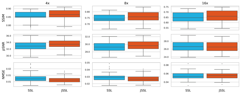
Figure S1: Evaluation metric results for SSL and JSSL methods using an image domain U-Net architecture as a reconstruction network.

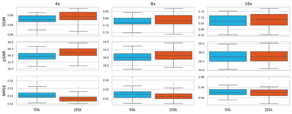
Figure S2: Evaluation metric results for SSL and JSSL methods using an E2EVarNet architecture as a reconstruction network.

The results of our supplementary comparative studies are depicted via box plots in Figures S1 and S2 for U-Net and E2EVarNet, respectively. Corresponding average metrics are provided in Tables S2 and S3.

From the results in Figures S1 and S2 and Tables S2 and S3, we observe alignment with our findings in Section 5 of the main paper: JSSL-trained models consistently outperform SSL-trained models for both architecture choices.

Furthermore, the superior performance of physics-driven models such as vSHARP (employed in the main paper) and E2EVarNet, over the U-Net model under both SSL and JSSL settings across all acceleration factors, advocates for the adoption of physics-informed models for reconstruction.

Appendix D Additional Figures

D.1 Comparison Studies

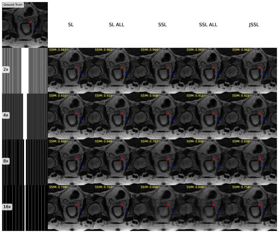
Figure S3: Example reconstructions of a slice subsampled at different acceleration factors (left-most column) from the test set from each training setup in the comparison studies (Section 5.2 of the main paper) visualized against the ground truth. Arrows point to regions of interest.

D.2 Ablation Studies

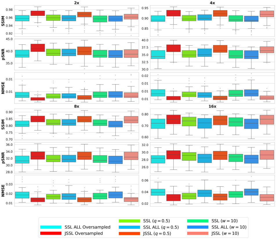
Figure S4: Evaluation results for varying JSSL and SSL setups for the ablation studies of Section 5.3 of the main paper.

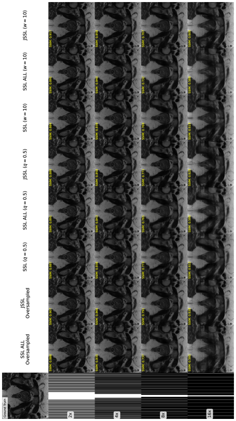
Figure S5: Example 1 of reconstructions of a slice subsampled at different acceleration factors (left-most column) from the test set from each training setup in the ablation studies (Section 5.3 of the main paper) visualized against the ground truth. Arrows point to regions of interest.

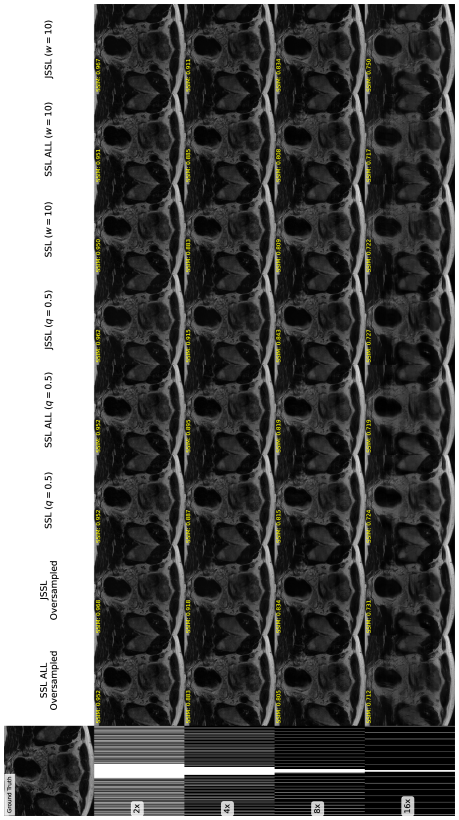
Figure S6: Example 2 of reconstructions of a slice subsampled at different acceleration factors (left-most column) from the test set from each training setup in the ablation studies (Section 5.3 of the main paper) visualized against the ground truth. Arrows point to regions of interest.

References

- [1] E.J. Candes, J. Romberg, and T. Tao. Robust uncertainty principles: exact signal reconstruction from highly incomplete frequency information. IEEE Transactions on Information Theory, 52(2):489–509, 2006.
- [2] Zhuo-Xu Cui, Chentao Cao, Shaonan Liu, Qingyong Zhu, Jing Cheng, Haifeng Wang, Yanjie Zhu, and Dong Liang. Self-score: Self-supervised learning on score-based models for mri reconstruction, 2022.
- [3] Jeffrey A Fessler. Optimization methods for mr image reconstruction, 2019.
- [4] Mark A. Griswold, Peter M. Jakob, Robin M. Heidemann, Mathias Nittka, Vladimir Jellus, Jianmin Wang, Berthold Kiefer, and Axel Haase. Generalized autocalibrating partially parallel acquisitions (GRAPPA). Magnetic Resonance in Medicine, 47(6):1202–1210, June 2002.
- [5] Kerstin Hammernik, Teresa Klatzer, Erich Kobler, Michael P. Recht, Daniel K. Sodickson, Thomas Pock, and Florian Knoll. Learning a variational network for reconstruction of accelerated MRI data. Magnetic Resonance in Medicine, 79(6):3055–3071, Nov. 2017.
- [6] Chen Hu, Cheng Li, Haifeng Wang, Qiegen Liu, Hairong Zheng, and Shanshan Wang. Self-supervised learning for MRI reconstruction with a parallel network training framework. In Medical Image Computing and Computer Assisted Intervention – MICCAI 2021, pages 382–391. Springer International Publishing, 2021.
- [7] Eu Hyun Kim, Moon Hyung Choi, Young Joon Lee, Dongyeob Han, Mahmoud Mostapha, and Dominik Nickel. Deep learning-accelerated t2-weighted imaging of the prostate: Impact of further acceleration with lower spatial resolution on image quality. European Journal of Radiology, 145:110012, Dec. 2021.
- [8] Diederik P. Kingma and Jimmy Ba. Adam: A method for stochastic optimization, 2017.
- [9] Yilmaz Korkmaz, Tolga Cukur, and Vishal M. Patel. Self-supervised MRI reconstruction with unrolled diffusion models. In Lecture Notes in Computer Science, pages 491–501. Springer Nature Switzerland, 2023.
- [10] Dong Liang, Jing Cheng, Ziwen Ke, and Leslie Ying. Deep magnetic resonance image reconstruction: Inverse problems meet neural networks. IEEE Signal Processing Magazine, 37(1):141–151, Jan. 2020.
- [11] Michael Lustig, David L. Donoho, Juan M. Santos, and John M. Pauly. Compressed sensing mri. IEEE Signal Processing Magazine, 25(2):72–82, 2008.
- [12] Charles A. McKenzie, Ernest N. Yeh, Michael A. Ohliger, Mark D. Price, and Daniel K. Sodickson. Self-calibrating parallel imaging with automatic coil sensitivity extraction. Magnetic Resonance in Medicine, 47(3):529–538, 2002.
- [13] Charles Millard and Mark Chiew. A theoretical framework for self-supervised mr image reconstruction using sub-sampling via variable density noisier2noise, 2023.
- [14] Arghya Pal and Yogesh Rathi. A review and experimental evaluation of deep learning methods for MRI reconstruction. J. Mach. Learn. Biomed. Imaging, 1, Mar. 2022.
- [15] Klaas P. Pruessmann, Markus Weiger, Markus B. Scheidegger, and Peter Boesiger. SENSE: Sensitivity encoding for fast MRI. Magnetic Resonance in Medicine, 42(5):952–962, Nov. 1999.
- [16] Saiprasad Ravishankar and Yoram Bresler. Mr image reconstruction from highly undersampled k-space data by dictionary learning. IEEE Transactions on Medical Imaging, 30(5):1028–1041, 2011.
- [17] Olaf Ronneberger, Philipp Fischer, and Thomas Brox. U-net: Convolutional networks for biomedical image segmentation. In Lecture Notes in Computer Science, pages 234–241. Springer International Publishing, 2015.
- [18] Manoj Sarma, Peng Hu, Stanislas Rapacchi, Daniel Ennis, Albert Thomas, Percy Lee, Patrick Kupelian, and Ke Sheng. Accelerating dynamic magnetic resonance imaging (MRI) for lung tumor tracking based on low-rank decomposition in the spatial-temporal domain: a feasibility study based on simulation and preliminary prospective undersampled MRI. Int. J. Radiat. Oncol. Biol. Phys., 88(3):723–731, Mar. 2014.
- [19] C.E. Shannon. Communication in the presence of noise. Proceedings of the IRE, 37(1):10–21, 1949.
- [20] Dilbag Singh, Anmol Monga, Hector L. de Moura, Xiaoxia Zhang, Marcelo V. W. Zibetti, and Ravinder R. Regatte. Emerging trends in fast mri using deep-learning reconstruction on undersampled k-space data: A systematic review. Bioengineering, 10(9), 2023.
- [21] Anuroop Sriram, Jure Zbontar, Tullie Murrell, Aaron Defazio, C. Lawrence Zitnick, Nafissa Yakubova, Florian Knoll, and Patricia Johnson. End-to-End Variational Networks for Accelerated MRI Reconstruction, page 64–73. Springer International Publishing, 2020.
- [22] Radhika Tibrewala, Tarun Dutt, Angela Tong, Luke Ginocchio, Mahesh B Keerthivasan, Steven H Baete, Sumit Chopra, Yvonne W Lui, Daniel K Sodickson, Hersh Chandarana, and Patricia M Johnson. Fastmri prostate: A publicly available, biparametric mri dataset to advance machine learning for prostate cancer imaging, 2023.
- [23] Martin Uecker, Peng Lai, Mark J. Murphy, Patrick Virtue, Michael Elad, John M. Pauly, Shreyas S. Vasanawala, and Michael Lustig. ESPIRiT-an eigenvalue approach to autocalibrating parallel MRI: Where SENSE meets GRAPPA. Magnetic Resonance in Medicine, 71(3):990–1001, May 2013.
- [24] Martin Uecker, Shuo Zhang, Dirk Voit, Alexander Karaus, Klaus-Dietmar Merboldt, and Jens Frahm. Real-time MRI at a resolution of 20 ms. NMR in Biomedicine, 23(8):986–994, Aug. 2010.
- [25] Burhaneddin Yaman, Seyed Amir Hossein Hosseini, Steen Moeller, Jutta Ellermann, Kâmil Uğurbil, and Mehmet Akçakaya. Self-supervised learning of physics-guided reconstruction neural networks without fully sampled reference data. Magnetic Resonance in Medicine, 84(6):3172–3191, July 2020.
- [26] George Yiasemis, Nikita Moriakov, Jan-Jakob Sonke, and Jonas Teuwen. Deep cardiac mri reconstruction with admm. arXiv.org, Oct 2023. arXiv:2310.06628 [eess.IV].
- [27] George Yiasemis, Nikita Moriakov, Jan-Jakob Sonke, and Jonas Teuwen. vsharp: variable splitting half-quadratic admm algorithm for reconstruction of inverse-problems. arXiv.org, Sep 2023. arXiv:2309.09954 [eess.IV].
- [28] George Yiasemis, Jan-Jakob Sonke, Clarisa Sánchez, and Jonas Teuwen. Recurrent variational network: A deep learning inverse problem solver applied to the task of accelerated mri reconstruction. In Proceedings of the IEEE/CVF Conference on Computer Vision and Pattern Recognition (CVPR), pages 732–741, June 2022.
- [29] George Yiasemis, Clara I. Sánchez, Jan-Jakob Sonke, and Jonas Teuwen. On retrospective k-space subsampling schemes for deep mri reconstruction. arXiv.org, Aug 2023. arXiv:2301.08365 [eess.IV].
- [30] Jure Zbontar, Florian Knoll, Anuroop Sriram, Tullie Murrell, Zhengnan Huang, Matthew J. Muckley, Aaron Defazio, Ruben Stern, Patricia Johnson, Mary Bruno, Marc Parente, Krzysztof J. Geras, Joe Katsnelson, Hersh Chandarana, Zizhao Zhang, Michal Drozdzal, Adriana Romero, Michael Rabbat, Pascal Vincent, Nafissa Yakubova, James Pinkerton, Duo Wang, Erich Owens, C. Lawrence Zitnick, Michael P. Recht, Daniel K. Sodickson, and Yvonne W. Lui. fastmri: An open dataset and benchmarks for accelerated mri, 2019.
- [31] Bo Zhou, Neel Dey, Jo Schlemper, Seyed Sadegh Mohseni Salehi, Chi Liu, James S. Duncan, and Michal Sofka. Dsformer: A dual-domain self-supervised transformer for accelerated multi-contrast mri reconstruction, 2022.