Abstract

Scalarized black holes (BH) have been shown to form dynamically in extended-scalar-tensor theories, either through spontaneous scalarization – when the BH is unstable against linear perturbations – or through a non-linear scalarization. In the latter, linearly stable BHs can ignite scalarization when sufficiently perturbed. These phenomena are, however, not incompatible and mixed scalarization is also possible. The objective of this work is twofold: first, study mixed scalarization on a family of Einstein-Maxwell-scalar models; and second, study the effect of the counter scalarization that occurs when one of the coupling parameters has a sign opposite to the one that generates scalarization. Both objectives are addressed by constructing and examining the mixed scalarization’s domain of existence. An overall dominance of the spontaneous scalarization over the non-linear scalarization is observed. Thermodynamically, an entropical preference for mixed over the standard scalarization (spontaneous or non-linear) exists. In the presence of counter scalarization, a quench of the scalarization occurs, mimicking the effect of a scalar particle’s mass/positive self-interaction term.

1 Introduction

With the recent observational data from the LIGO-VIRGO collaboration (e.g. [1, 2]) and the direct imaging by the Event Horizon Telescope [3, 4], a heightened interest in alternative black hole (BH) solutions has emerged.

Of particular interest are hairy black hole solutions (see [5] for a review) resulting from a scalarization process (aka scalarized BHs).

A possible mechanism of scalarization occurs in extended-scalar-tensor theories (eST) [6]. In these, the scalar field non-minimally couples to the model’s invariant and scalar perturbations of the vacuum BH can ignite the growth of scalar hair around the BH. The resulting objects may present significant deviations when compared with the standard vacuum General relativity (GR) solutions, which can give a better insight into the nature of gravity and particle physics.

A family of eST theories that have undergone extensive analysis is the Einstein-Maxwell-Scalar (EMS) model [7, 8, 9, 10, 11, 12, 13, 14, 15, 16, 17, 18, 19, 20, 21]. In the latter, scalarization is triggered by a non-minimal coupling between a real scalar field, $\phi$, and the Maxwell invariant, $\mathcal{I}=F_{\mu\nu}F^{\mu\nu}$, through a coupling function $f(\phi)$

$$\mathcal{S}=\int d^{4}x\sqrt{-g}\left[R-2\,\partial_{\mu}\phi\partial^{\mu}\phi-f(\phi)\mathcal{I}\right]\ ,$$ (1)

and minimally coupled with the Ricci scalar, $R$, associated with the metric ansatz $g_{\mu\nu}$. Scalarization is triggered by a sufficiently large charge-to-mass ratio.

Although BHs within this model are considered of less astrophysical significance compared to those in other eST models such as the Scalar-Gauss-Bonnet [23, 24, 25], their relative computational simplicity has proven valuable to developing a better insight into the scalarization phenomenon [26, 27, 28, 29, 30, 31, 32, 33, 34, 35, 36, 37, 38, 39, 40, 41].

In particular, the simplicity associated with the EMS model has allowed the study of several coupling functions [8, 42, 43], from which two classes of solutions were found: class I (or dilatonic-type) and class II (aka scalarization type). While in the former $\phi=0$ does not solve the field equation , in the latter, the trivial scalar field does solve the field equation and scalarized solutions can result from perturbations of the vacuum BH solution . This demands that

$$\frac{df(\phi)}{d\phi}\bigg{|}_{\phi=0}=0\ .$$ (2)

This condition is naturally implemented, for instance, if one requires the model to be $\mathbb{Z}_{2}$-invariant under $\phi\rightarrow-\phi$. Scalarized solutions can be further divided into two sub-classes.

When vacuum BH are unstable against linear perturbations, a tachyonic instability arises when

$$\frac{d^{2}f(\phi)}{d\phi^{2}}\bigg{|}_{\phi=0}\neq 0\ ,$$ (3)

and with the opposite sign of $\mathcal{I}$. The scalar hair around the BH grows spontaneously from a perturbed vacuum Reissner-Nordstrom BH (RN BH). In this case, the scalarized solutions bifurcate from the vacuum RN BH solutions. These are known as class II.A or spontaneous/normal scalarization.

A second family of scalarized solutions, class II.B or non-linear scalarization, is also possible when the BH is stable against linear perturbations,

$$\frac{d^{2}f(\phi)}{d\phi^{2}}\bigg{|}_{\phi=0}=0\ ,$$ (4)

but unstable against non-linear perturbations. In this case, a sufficiently large non-linear perturbation can trigger the growth of the scalar hair of the vacuum BH.

These two scalarization types are, however, not incompatible and mixed scalarization is also possible [44]. A coupling function compatible with both spontaneous and non-linear scalarization is

$$f(\phi)=e^{-\alpha\phi^{2}-\beta\phi^{4}}\ ,$$ (5)

with $\alpha<0$ and $\beta<0$. The sign of the coupling parameters $(\alpha,\ \beta)$ was chosen in accordance with the literature. Pure – aka non-mixed – spontaneous (non-linear) scalarization being recovered when $\beta=0$ ($\alpha=0$).

The existence of scalarization is highly dependent on the sign of the spontaneous/non-linear function parameters ($\alpha,\,\beta$). While for pure scalarization the sign of either parameter is well defined, the presence of an additional scalarization mechanism, say spontaneous scalarization ($\alpha$), allows $\beta$ to have the “wrong” sign. We call this counter-scalarization.

The objective of this work is twofold: first, to study the interplay between spontaneous and non-linear scalarization in the mixed scalarization scenario; second, to examine the effects of incorporating a counter-scalarization term into the coupling function.

The paper is organized as follows: Sec. 2 introduces the basics of the EMS model, including a description of the equations of motion, boundary conditions, and relevant relations. Sec. 3 is dedicated to the numerical results. These include the computation of the domain of existence, Sec. 3.2, and both the entropical, Sec. 3.2, and perturbative, Sec. 3.3, stabilities. The paper concludes with some final remarks in Sec. 4.

Throughout this paper, we set $4\pi G=1=4\pi\epsilon_{0}$ for convenience. The spacetime signature is chosen to be $(-,+,+,+)$. We focus exclusively on spherically symmetric solutions, which implies that the metric and matter functions depend solely on the radial coordinate. For simplicity in notation, once a function is introduced with its radial dependency, such as $X(r)$, we will subsequently denote it by $X$ with the understanding that it is a function of $r$. Derivatives with respect to the radial coordinate $r$ and the scalar field $\phi$ are represented by $X^{\prime}\equiv\frac{dX}{dr}$ and $X_{,\phi}\equiv\frac{dX}{d\phi}$, respectively.

2 The EMS model

As already stated in the Introduction (Sec. 1), in this work we are going to restrict ourselves to spherically symmetric EMS models described by action (1). For the line element, let us consider a standard metric ansatz that is compatible with spherical symmetry and has two unknown functions

$$ds^{2}=-N(r)e^{-2\delta(r)}dt^{2}+\frac{dr^{2}}{N(r)}+r^{2}\big{(}d\theta^{2}+\sin^{2}\theta\,d\varphi^{2}\big{)}\ ,~{}~{}{\rm with}~{}~{}N(r)\equiv 1-\frac{2\,m(r)}{r},$$ (6)

where $m(r)$ is the Misner-Sharp mass function [49] and $\delta(r)$ is an unknown metric function. Spherical symmetry, in the absence of a magnetic charge, imposes an electrostatic $4-$vector potential, $A(r)=V(r)\,dt$, and a scalar field solely radial dependent, $\phi(t,r,\theta,\varphi)\equiv\phi(r)$. The absence of angular dependence allows one to obtain the effective Lagrangian,

$$\mathcal{L}_{\rm eff}=e^{-\delta}m^{\prime}-\frac{1}{2}r^{2}e^{-\delta}N\phi^{\prime 2}+\frac{1}{2}f(\phi)e^{\delta}r^{2}V^{\prime 2}\ .$$ (7)

Variation of the effective Lagrangian with respect to the metric and matter functions yields the field equations:

$$m^{\prime}=\frac{r^{2}N\phi^{\prime 2}}{2}+\frac{Q^{2}}{2r^{2}f(\phi)}\ ,\qquad\delta^{\prime}+r\phi^{\prime 2}=0\ ,\qquad V^{\prime}=-\frac{Qe^{-\delta}}{f(\phi)r^{2}}\ ,$$ (8)

$$\phi^{\prime\prime}+\frac{1+N}{rN}\phi^{\prime}-\frac{Q^{2}}{r^{3}Nf(\phi)}\left(\phi^{\prime}-\frac{f_{,\phi}(\phi)}{2rf(\phi)}\right)=0\ .$$

Where the electrostatic potential $V$ is under a first integral which was used to simplify the remaining equations. The constant of integration is interpreted as the electric charge, $Q$.

To solve the set of four coupled ordinary differential equations (8), one must implement the appropriate boundary conditions. At the horizon, $r=r_{H}$, the field equations can be approximated by a power series expansion in $r-r_{H}$ as

$$m=\frac{r_{H}}{2}+\frac{Q^{2}}{2r_{H}^{2}f(\phi_{0})}(r-r_{H})+\cdots\ \ ,\qquad\delta=\delta_{0}-r_{H}\bigg{(}\frac{Q^{2}}{2r_{H}\big{(}Q^{2}-r_{H}^{2}f(\phi_{0})\big{)}}\frac{f_{,\phi}(\phi_{0})}{f(\phi_{0})}\bigg{)}^{2}\,(r-r_{H})+\cdots\ ,$$ (9)

$$\phi=\phi_{0}+\frac{Q^{2}f_{,\phi}(\phi_{0})}{2r_{H}f(\phi_{0})\big{(}Q^{2}-r_{H}^{2}f(\phi_{0})\big{)}}(r-r_{H})+\cdots\ ,\qquad\qquad\ \ \ \ \ V=-\frac{e^{-\delta_{0}}Q}{r_{H}^{2}f(\phi_{0})}(r-r_{H})+\cdots\ ,$$

in terms of the two essential parameters $\phi_{0}$ and $\delta_{0}$, where the subscript ₀ denotes functions evaluated at the horizon $r_{H}$. At spatial infinity, asymptotic flatness is ensured by a power series expansion in $1/r$.

$$m(r)=M-\frac{Q^{2}+Q_{s}^{2}}{2r}+\cdots\ ,\qquad\qquad\qquad\delta(r)\approx\frac{Q_{s}^{2}}{2\,r^{2}}+\cdots\ ,$$ (10)

$$\phi(r)=\frac{Q_{s}}{r}+\frac{MQ_{s}}{r^{2}}+\cdots\ ,\qquad\qquad\qquad\quad V(r)=\psi_{e}+\frac{Q}{r}+\cdots\ ,$$

with $M$ representing the ADM mass, $Q$ the BH’s electric charge, and $Q_{s}$ the scalar “charge”, while $\psi_{e}$ is the electrostatic potential at infinity.

Equation (8), together with the boundary conditions arising from the power series expansion (9) and (10), constitute a Dirichlet boundary condition problem that must be numerically integrated (see Sec. 3).

2.1 Identities and physical quantities of interest

Scalarized solutions are physically characterised by the dimensionless quantities: charge-to-mass ratio, $q$, reduced horizon area, $a_{H}$, and reduced horizon temperature, $t_{H}$,

$$q\equiv\frac{Q}{M}\ ,\qquad a_{H}\equiv\frac{A_{H}}{16\pi M^{2}}=\frac{r_{H}^{2}}{4M^{2}}\ ,\qquad t_{H}\equiv 8\pi MT_{H}=2MN^{\prime}(r_{H})e^{-\delta_{0}}\ \ ,$$ (11)

where $A_{H}=4\pi r_{H}^{2}$ and $T_{H}=N^{\prime}(r_{H})e^{-\delta_{0}}/4\pi$ are the area and temperature of the BH’s horizon, respectively. Regularity of the solutions is guaranteed by the Ricci scalar, $R$, and the Kretschmann scalar, $K\equiv R_{\mu\nu\delta\lambda}R^{\mu\nu\delta\lambda}$,

$$R =\frac{N^{\prime}}{r}\big{(}3\,r\,\delta^{\prime}-4\big{)}+\frac{2}{r^{2}}\Big{\{}1+N\Big{[}r^{2}\delta^{\prime\prime}-\big{(}1-r\delta^{\prime}\big{)}^{2}\Big{]}\Big{\}}-N^{\prime\prime}\ ,$$ (12)

$$K =\frac{4}{r^{4}}\big{(}1-N\big{)}^{2}+\frac{2}{r^{2}}\left[N^{\prime\,2}+\big{(}N^{\prime}-2N\delta^{\prime}\big{)}^{2}\right]+\left[N^{\prime\prime}-3\,\delta^{\prime}N^{\prime}+2N\big{(}\delta^{\prime\,2}-\delta^{\prime\prime}\big{)}\right]^{2}\ .$$

Physical accuracy is ensured through the so-called virial identity, Smarr law and non-linear Smarr relation. The virial identity is obtained through a Derrick-like scaling argument [50, 51, 52, 53] and is given by

$$\int_{r_{H}}^{\infty}dr\left\{e^{-\delta}\,r^{2}\,\phi^{\prime\,2}\left[1+\frac{2\,r_{H}}{r}\bigg{(}\frac{m}{r}-1\bigg{)}\right]\right\}=\int_{r_{H}}^{\infty}dr\left[e^{-\delta}\left(1-\frac{2\,r_{H}}{r}\right)\frac{1}{r^{2}}\frac{Q^{2}}{f(\phi)}\right]\ ,$$ (13)

which is independent of the equations of motion and displays that scalarization can occur only in the presence of an electric charge $Q\neq 0$ in an EMS model .

The Smarr law for this family of solutions is found not to be explicitly dependent on the scalar field:

$$M=\frac{1}{2}T_{H}A_{H}+\psi_{e}Q\ .$$ (14)

The first law of black hole thermodynamics for EMS black holes is expressed as

$$dM=\frac{1}{4}T_{H}\,dA_{H}+\psi_{e}\,dQ\ .$$ (15)

At last, it can be shown that scalarized solutions also obey the so-called non-linear Smarr formula [8],

$$M^{2}+Q_{s}^{2}=Q^{2}+\frac{1}{4}A_{H}^{2}T_{H}^{2}\ .$$ (16)

2.2 Coupling function

As previously mentioned, the choice of the coupling function is crucial in determining whether the RN BH is susceptible to scalarization, and hence one should be careful in designing the coupling function. Let us recap the conditions for scalarization. The first requirement is that the GR BH solution should also be a solution within the EMS model. Analysis of the field equations (8) shows that this can be secured by imposing (2). This condition is naturally implemented if one requires the model to be $\mathbb{Z}_{2}-$invariant under the transformation $\phi\rightarrow-\phi$. The type of scalarization, on the other hand, is controlled by the second derivative of $f(\phi)$. For this, it is important to recall that the scalar field is described by the Klein-Gordon equation

$$\Box\phi=\frac{\mathcal{I}}{4}f_{,\phi}.$$ (17)

Let us now consider a small-$\phi$ expansion of the coupling function

$$f(\phi)=f(0)+\frac{1}{2}\frac{d^{2}f}{d\phi^{2}}\bigg{|}_{\phi=0}\phi^{2}+\cdots\ ,$$ (18)

the Klein-Gordon equation (17) linearized for small-$\phi$ reads:

$$\big{(}\Box-\mu_{\rm eff}^{2}\big{)}\phi=0\ ,\qquad{\rm where}\qquad\mu_{\rm eff}^{2}=\mathcal{I}\,\frac{d^{2}f(\phi)}{d\phi^{2}}\bigg{|}_{\phi=0}\ .$$ (19)

The instability arises if the scalar field’s effective mass $\mu_{\rm eff}^{2}<0$ (aka tachyonic mass), which, in particular, requires $f_{,\phi\phi}$ to obey (3) and with the opposite sign of $\mathcal{I}$. This constitutes the set of solutions known as normal/spontaneous scalarization associated with class II.A, of which an exemplary function is

$$f(\phi)=e^{-\alpha\phi^{2}}\ ,$$ (20)

Class II.B on the other hand, occurs when solutions are always linearly stable and no tachyonic instability exists, i.e. for (4). This condition is easily satisfied by considering higher order terms in the expansion of $f(\phi)$ such as

$$f(\phi)=e^{-\beta\phi^{4}}\ .$$ (21)

An exemplary function that exhibits, simultaneously, the tachyonic and non-linear instabilities is the previously introduced (5), $f(\phi)=e^{-\alpha\phi^{2}-\beta\phi^{4}}$. Observe that, due to the presence of non-linear (linear) scalarization in the coupling function, scalarized BHs in the EMS model can incorporate a counteracting linear (non-linear) term.

In particular, it is feasible to have scalarized solutions with $\alpha>0$ supported by the non-linear term $\beta<0$; or a scalarized solution with $\beta>0$ supported by the tachyonic (linear) instability $\alpha<0$.

Analysis of (19) reveals that these counteracting terms do not contribute to scalarization. Instead, they can be interpreted as a mass term for the scalar field – in the case of the linear term $\alpha>0$ –, or as a positive quartic self-interaction – for $\beta>0$ –, both proportional to the BH’s electric charge due to the non-minimal coupling between the scalar field and the Maxwell invariant. Investigation of the latter’s impact on the scalarization phenomena constitutes the second objective of this work.

3 Numerical results

The set of four coupled ODEs (8), with the proper boundary conditions (9)-(10), are solved numerically. The chosen routines automatically impose the proper boundary conditions through a shooting method on the two unknown parameters $\phi_{0}$ and $\delta_{0}$, with the maximum integration error and boundary conditions automatically ensured to be less than $10^{-15}$.

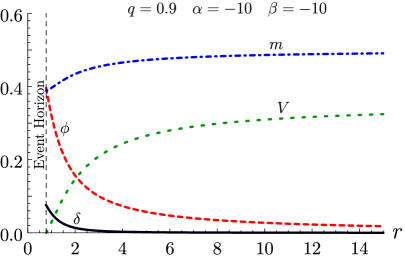
Figure 1: Radial profile of the scalar field, $\phi$, metric, $(m,\,\delta)$, and energy density, $\rho$, of a mixed scalarized BH solutions with $r_{H}=0.78$, $\phi_{0}=0.40$ and $q=0.90$ and coupling parameters $\alpha=-10.0$ and $\beta=-10.0\,$.

Physical accuracy is guaranteed through the virial identity, with a relative error of $10^{-6}$, and Smarr and non-linear Smarr relations, with a relative error of $10^{-7}$. The resulting numerical solution’s profile can be seen in Fig. 1 for an exemplary solution with $r_{H}=0.78$, $\phi_{0}=0.40$ and $q=0.90$ and coupling parameters $\alpha=-10.0$ and $\beta=-10.0\,$.

All obtained solutions are everywhere regular at and outside the horizon, $r_{H}$. Each scalarized BH solution is uniquely defined by $(r_{H},\,\alpha,\,\beta,\,q)$.

3.1 Domain of existence

Variation of the horizon radius, $r_{H}$, and coupling parameters, $(\alpha,\,\beta)$, for a fixed electric charge $Q$, form the $3-$dimensional domain of existence that characterizes the EMS model under analysis. To avoid the additional complexity associated with the $3-$dimensional domain of existence, let us fix one of the coupling parameters (say $\alpha$) and vary the other ($\beta$) – see Fig. 2.

In Fig. 2 is graphically represented the projection of the domain of existence of a scalarized BH as a function of $\alpha$ for three values of $\beta=\{-10.0,\,0,\,+10.0\}$ (left panel); and as a function of $\beta$ for four values of $\alpha=\{-10.0,\,-1.0,\,0,\,+1.0\}$ (right panel).

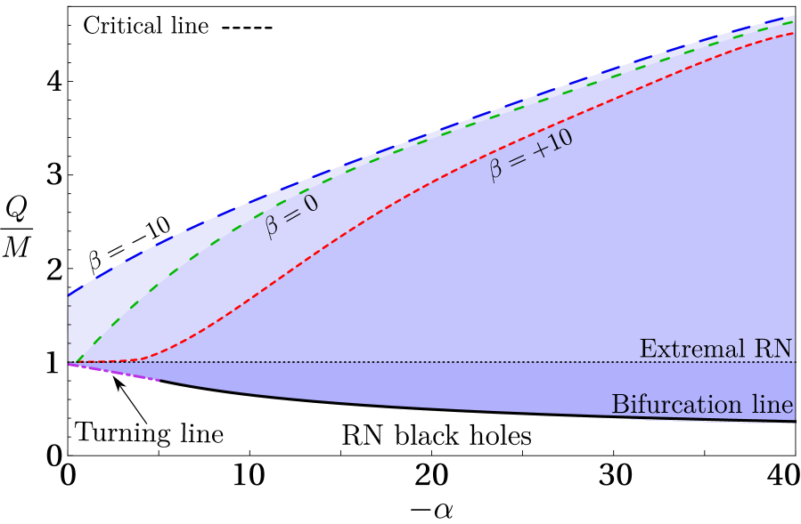
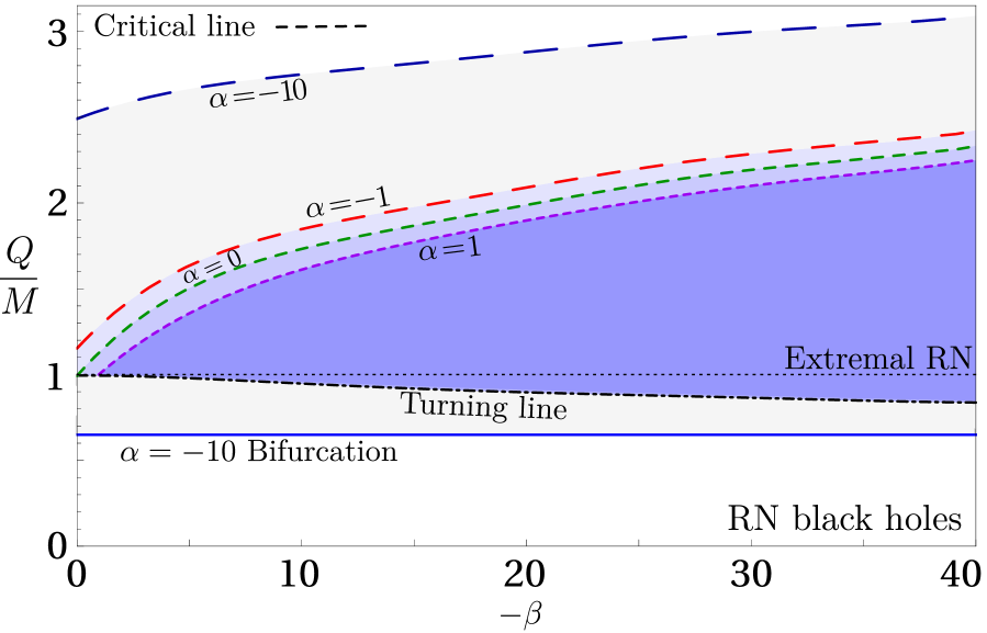
Figure 2: Domain of existence of scalarized BHs in EMS models (shaded blue regions) with coupling function $f(\phi)=e^{-\alpha\phi^{2}-\beta\phi^{4}}$ as a function of $\alpha$ with $\beta=\{-10.0,\,0,\,+10.0\}$ (left panel); or $\beta$ for $\alpha=\{-10.0,\,-1.0,\,0,\,+1.0\}$ (right panel). The domain of existence is bounded from below by the existence/turning line (solid/dot-dashed line) and from above by the critical line (dashed line).

A common feature of both domains of existence is a region with $q\leqslant 1$ – where degeneracy occurs– and a region with overcharged solutions $q>1$. The former region is limited from below by the bifurcation/turning line and from above by the extremal line $q=1$, and represents a region of the parameter space where, at least, two BH configurations with the same $q$ coexist: a bald RN BH and one or more scalarized BH solution. These solutions, however, possess different horizon radii (Fig. 3), temperatures and entropy (see Sec. 3.2).

The overcharged region goes from the extremal line, $q=1$, and is bounded from above by the critical line, which is highly coupling parameter’s dependent: $q_{crit.}\equiv q_{crit.}(\alpha,\beta)$. At the critical line, the solution’s horizon radius tends to zero, $r_{H}\to 0$. In this region, no bald RN BH exist and no degeneracy between scalarized BHs was observed. After the critical line, no solutions exist.

In addition, Fig. 2 demonstrates a dominance of the tachyonic instability over the non-linear scalarization: for the same value of $\beta$ and $\alpha$, the domain of existence is bounded from below by the bifurcation line and has a $q_{crit.}$ comparable to the pure spontaneous scalarization, $\beta=0.0\,$. Such is expected since the maximum of the scalar field amplitude occurs at the horizon (see Fig. 1) and is smaller than unity $max(phi)=\phi_{0}<1$, resulting in a decreased contribution of the higher powers of the scalar field.

The lower bound, however, depends on the relative value of $\alpha$ in relation to $\beta$. If $\beta\lesssim\alpha$, the scalarization is dominated by the tachyonic instability and the domain of existence is bounded from below by the bifurcation line; when $\beta\gg\alpha$, non-linear scalarization dominates and the domain of existence is bounded from below by the turning line (see Fig. 2). In this case, the tachyonic instability is not strong enough to sustain a negligible amount of scalar field (see Fig. 3), and a minimum value of $\phi_{0}$ exists. With the increase of $\alpha$, the size of the initial $\phi_{0}$ jump decreases until $\phi_{0}\to 0$ and the tachyonic instability dominates.

Let us now analyse the individual domains of existence. Starting with a fixed $\beta=\{-10.0,0.0,+10.0\}$ and vary $\alpha$ – see Fig. 2 (left panel). In the majority of the domain of existence, solutions bifurcate from the RN BH at $q\leqslant 1$ – where scalarized BHs with a negligibly amount of scalar field can exist – and stops at the critical line, $r_{H}\to 0$. In between a continuously monotonic increase of the scalar field amplitude at the horizon and a reduction of the latter occurs.

As expected, the bifurcation line is insensitive to the non-linear term since the bifurcation is only dependent on the linear terms of $f_{,\phi}(\phi)$ that enter into the rhs of the Klein-Gordon equation (17).

The critical line, on the other hand, is highly dependent on the coupling parameters. The maximum charge-to-mass ratio for which the critical solutions exist, $q_{crit.}$, increases/decreases with the addition of a negative/positive $\beta$ term. While for $\beta<0$, a non-linear instability that amplifies the scalarization exists, a positive value has the opposite effect. The $\beta>0$ decreases the width of the domain of existence due to a decrease in $q_{crit.}$, resulting in a quench of the scalarization similar to the one observed for scalarization with a positive self-interaction [54].

Observe now the case with fixed $\alpha=\{-10,-1,0,+1\}$ and varying $\beta$ – Fig. 2 (right panel). In this case, for all the chosen $\alpha\neq-10$, solutions start at the extremal line $q=1$ for which a minimal, non-negligible, amount of scalar field exists around the BH, $\phi_{0}\neq 0$. The BH’s scalar field’s associated jump high decreases (increases) with the addition of the $\alpha<0$ ($\alpha>0$) term (see also Fig. 3).

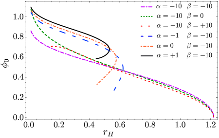
Figure 3: Scalar field horizon amplitude, $\phi_{0}$, as a function of the charge-to-mass ratio, $q$, for a mixed scalarized BH for six different coupling parameters configurations $(\alpha,\beta)$: (dot-dashed purple) mixed scalarization $(-10.0,-10.0)$; (dotted green) pure spontaneous scalarization $(-10.0,0.0)$; (dotted red) spontaneous scalarization $(-10.0,+10.0)$; (dashed blue) mixed scalarization with $(-1.0,-10.0)$; (dot-dashed orange) pure non-linear scalarization $(0.0,-10.0)$; mixed scalarization with $(+1.0,-10.0)$.

Following the initial jump in the scalar field amplitude at the horizon, solutions observe a simultaneous increase of $\phi_{0}$ and $r_{H}$ until a maximum mass, $r_{H}$ is reached – Fig. 3 $\beta=-10$ lines. After this point, a second branch with decreasing $r_{H}$ and increasing $\phi_{0}$ exists until the critical solution is achieved. The latter is known as the hot branch and is known to be stable for $\alpha=0$ [55, 56]; the former is known as the cold branch and is unstable (the denomination will be clear in the thermodynamics section 3.2).

As mentioned before, while the effect of a positive $\alpha$ is similar to scalarization by a massive scalar field, the positive $\beta$ mimics a positive self-interacting (attractive) potential. The present results follow the same pattern as the one presented for a massive/self-interacting scalar field in EMS [54, 57] and scalar-Gauss-Bonnet models [58, 59, 45]. In particular, a quench of the scalarization phenomena due to the decrease in the domain of existence width (see Fig. 2). However, due to the non-minimal coupling between the ”mass” or ”self-interaction” terms to the Maxwell invariant, the impact of the latter is proportional to the electric charge $Q$.

3.2 Thermodynamics

A solution is said to be stable if it is simultaneously entropically preferable and stable against radial perturbations. The latter will be studied in Sec. 3.3. In EMS models, entropy is given by the Bekeinstein-Hawking formula [60, 61, 62] and reduces to the analysis of the reduced horizon area, $a_{H}$, observe Fig. 4 (left panel).

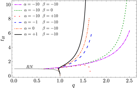
Figure 4: Reduced area, $a_{H}$, (left panel) and reduced horizon temperature, $t_{H}$, (right panel) as a function of the charge-to-mass ratio $q$ for a mixed scalarized BH with six different coupling parameter’s configurations $(\alpha,\beta)$: (dot-dashed purple) mixed scalarization $(-10.0,-10.0)$; (dotted green) pure spontaneous scalarization $(-10.0,0.0)$; (dotted red) spontaneous scalarization $(-10.0,+10.0)$; (dashed blue) mixed scalarization with $(-1.0,-10.0)$; (dot-dashed orange) pure non-linear scalarization $(0.0,-10.0)$; mixed scalarization with $(+1.0,-10.0)$.

Analysis of the horizon area shows that solutions dominated by spontaneous scalarization are always entropically preferable when compared with electro-vacuum GR; while non-linearly dominated solutions have a first branch that is everywhere entropically unfavourable (aka cold branch), and a second branch which contains a set of solutions that are entropically preferable (aka hot branch). The second branch’s entropically non-preferable region decreases (increases) with the addition of $\alpha<0$ ($\alpha>0$). The terminology hot/cold comes from the second branch having a higher temperature than the first, see Fig. 4 (right panel).

3.3 Comments on stability

Stability against radial perturbations is studied through a standard strategy that considers spherically symmetric, linear perturbations of the equilibrium solutions while keeping the metric ansatz (6), but allowing the functions $N,\,\delta,\,\phi,\,V$ time, $t$, dependent besides $r$:

$$ds^{2}=-\tilde{N}(r,t)\,e^{-2\,\tilde{\delta}(r,t)}dt^{2}+\frac{dr^{2}}{\tilde{N}(r,t)}+r^{2}\left(d\theta^{2}+\sin^{2}\theta\,d\varphi^{2}\right),\quad A=\tilde{V}(r,t)\,dt,\quad\phi=\tilde{\phi}(r,t)\ .$$ (22)

Each function can be further expanded into the equilibrium solution (aka “bare”) that where obtained previously (Sec. 3-3.2), plus a perturbation term. The latter contains the time-dependence through a Fourier mode with frequency $\Omega$,

$$\tilde{N}(r,t)=N(r)+\epsilon N_{p}(r)e^{-i\Omega t}\ ,\quad\tilde{\delta}(r,t)=\delta(r)+\epsilon\delta_{p}(r)e^{-i\Omega t}\ ,$$ (23)

$$\tilde{\phi}(r,t)=\phi(r)+\epsilon\phi_{p}(r)e^{-i\Omega t}\ ,\quad\tilde{V}(r,t)=V(r)+\epsilon V_{p}(r)e^{-i\Omega t}\ ,$$

where the subscript _p denotes perturbations of the equilibrium solutions. The linearized field equations around the background solution yield the metric and $V_{p}(r)$ perturbations expressed in terms of the scalar field perturbation, $\phi_{p}(r)$,

$$N_{p}=-2\,r\,N\phi^{\prime}\,\phi_{p}\ ,\qquad\delta_{p}=-2\int dr\,r\,\phi^{\prime}\phi_{p}^{\prime}\ ,\qquad V_{p}^{\prime}=-V^{\prime}\bigg{[}\delta_{p}+\phi_{p}\frac{f_{,\phi}(\phi)}{f(\phi)}\bigg{]}\ ,$$ (24)

This leads to a single perturbation equation for $\phi_{p}(r)$ which can be written in a Schrödinger-like form by redefining $\Psi(r)=r\,\phi_{p}$ and inserting the ’tortoise’ coordinate $x$ defined by $dx/dr=e^{\delta}/N$:

$$-\frac{d^{2}\Psi}{dx^{2}}+U_{\Omega}\Psi=\Omega^{2}\,\Psi\ ,$$ (25)

with the perturbation potential $U_{\Omega}$ defined as:

$$U_{\Omega}\equiv\frac{e^{-2\delta}N}{r^{2}}\left\{1-N-2\,r^{2}\phi^{\prime\,2}-\frac{Q^{2}}{2r^{2}}\left[\frac{2}{f(\phi)}\left(1-2\,r^{2}\phi^{\prime 2}\right)-\frac{2f_{,\phi}^{2}(\phi)}{f^{3}(\phi)}+\frac{1}{f^{2}(\phi)}\Big{(}f_{,\phi\phi}(\phi)+4\,r\,\phi^{\prime}f_{,\phi}(\phi)\Big{)}\right]\right\}$$ (26)

The potential $U_{\Omega}$, which is regular across the entire domain $-\infty<x<\infty$, diminishes to zero at both the black hole (BH) event horizon and infinity. A mode is classified as unstable if $\Omega^{2}<0$, which, within the asymptotic boundary conditions of our framework, indicates a bound state. However, a standard quantum mechanical result dictates that equation (25) will not exhibit bound states if $U_{\Omega}$ consistently exceeds its minimal asymptotic value, implying it must be positive (see e.g. [63]). Therefore, a uniformly positive effective potential serves as evidence of mode stability against spherical perturbations.

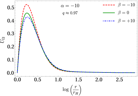
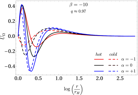
Figure 5: Effective potential for a set of scalarized RN BH solutions. (Left panel) Spontaneous scalarized dominated solutions with $\alpha=-10.0$ and (dashed red) $\beta=-10.0$ mixed scalarization, (solid green) $\beta=0.0$ pure spontaneous scalarization, and (dot-dashed blue) $\beta=+10.0$ counter-non-linear. (Right panel) non-linear scalarization dominated solutions with $\beta=-10.0$ for both hot (solid) and cold (dashed) branches with (red) $\alpha=-1.0$ mixed scalarization, (black) $\alpha=0$ pure non-linear scalarization, and (blue) $\alpha=+1.0$ counter-spontaneous scalarization.

To discern the interplay between the parameters $\alpha$ and $\beta$ on the effective potential, we analyzed the profile of $U_{\Omega}$ for several scalarized solutions, holding $\alpha$ constant while varying $\beta$ – Fig. 5 (left panel)–, and vice-versa – Fig. 5 (right panel).

The effective potential for radial spherical perturbations of spontaneously scalarized dominated solutions corresponding to a fixed $\alpha=-10.0$ – Fig. 5 (left panel) –, exhibit an everywhere positive effective potential, $U_{\Omega}>0$, suggesting the absence of instabilities. Additionally, one observes an increase (decrease) of the maximum value of $U_{\Omega}$ with the addition of the non-linear (counter-non-linear) parameter $\beta$.

In the case of non-linearly dominated scalarized solutions with fixed $\beta=-10.0$ – Fig. 5 (right panel) –, for both the hot and cold branches, a region where $U_{\Omega}$ changes sign exists. Which, while not indicating instabilities, doesn’t guarantee stability.

The addition of a tachyonic term, $\alpha=-1.0$, to the non-linearly dominated scalarized solution reduces the amplitude of the negative $U_{\Omega}$ region, bringing it closer to the stable spontaneously lead scalarization, while a counter-scalarized term $\alpha=+1.0$ deepens it.

At last, it is important to note that a non-uniformly positive potential for the non-linear scalarized solutions is not a guarantee of instabilities. To further investigate these solutions, the application of more intricate methods like the S-deformation method [64, 65, 66] is required. Such is beyond the scope of this paper (see [55] for a similar study of the pure non-linear scalarization, and [54, 57] for the impact of self-interacting/mass term).

4 Conclusions

In this work, we have investigated the interplay between the spontaneous and non-linear scalarization of charged black holes within the Einstein-Maxwell-Scalar model. The resulting mixed scalarized solutions possess both properties of pure non-linear and spontaneous scalarization.

The interplay between the two types of scalarization shows a dominance of the spontaneus properties over the non-linear ones. In particular, the domain of existence for comparable coupling parameters possesses the same structure of the spontaneous scalarization with a slight increase in the width from the non-linear scalarization. The influence of non-linear scalarization becomes apparent only when its coupling parameter is significantly larger than that of spontaneous scalarization.

The tachyonic instability associated with the spontaneous scalarization in the mixed coupling makes the black hole more susceptible to scalarization. As a result, it requires a weaker coupling of the scalar field to the Maxwell invariant to achieve the same level of scalarization.

The presence of a mixed scalarization also allowed the study of a “counter-scalarization´´ term, wherein one of the scalarization parameters has the “wrong´´ sign and, instead of supporting/intensifying the scalarizaton, suppresses it. From the linearized KG equation, one observes that these terms possess the properties of a scalar field’s mass (for the linear parameter $\alpha>0$) or of a positive self-interaction (for the non-linear $\beta>0$). The resulting quench associated with these parameters mimics the effect of a scalar field’s mass/self-interaction observed in previous studies [54, 57]. However, due to the coupling to the Maxwell invariant, the effect is not constant.

Thermodynamically, mixed scalarized solutions with higher negative values of both $\alpha$ and $\beta$ are favourable. Solutions dominated by spontaneous scalarization are entropically preferable over their General Relativity counterparts, while non-linear dominated solutions show mixed thermodynamic behaviour, i.e. an entropically favourable and unfavourable regions.

Perturbative stability analysis against radial perturbations indicated stability for dominant spontaneously scalarized black holes. In contrast, for non-linear dominated scalarization, such a conclusion is not possible to be made. Further studies into these must be made.

However, it seems like the addition of the spontaneous scalarization parameter to the non-linear scalarization makes the resulting mixed scalarization tend to a more stable configuration.

Future research directions include applying the S-Deformation method for an in-depth analysis of the radial stability of non-linearly dominated solutions. A comprehensive study of quasi-normal modes in mixed scalarized solutions could provide further insights extending the work of [67, 56, 68, 69]. Additionally, incorporating rotation into these mixed scalarization configurations presents an intriguing avenue for exploration.

References

- [1] B. P. Abbott, R. Abbott, T. Abbott, M. Abernathy, F. Acernese, K. Ackley, C. Adams, T. Adams, P. Addesso, R. Adhikari, et al., “Observation of gravitational waves from a binary black hole merger,” Physical review letters, vol. 116, no. 6, p. 061102, 2016.
- [2] R. Abbott, T. Abbott, S. Abraham, F. Acernese, K. Ackley, A. Adams, C. Adams, R. Adhikari, V. Adya, C. Affeldt, et al., “Gwtc-2: compact binary coalescences observed by ligo and virgo during the first half of the third observing run,” Physical Review X, vol. 11, no. 2, p. 021053, 2021.
- [3] D. Ball, C.-k. Chan, P. Christian, B. T. Jannuzi, J. Kim, D. P. Marrone, L. Medeiros, F. Ozel, D. Psaltis, M. Rose, et al., “First m87 event horizon telescope results. i. the shadow of the supermassive black hole,” IOP PUBLISHING LTD, 2019.
- [4] K. Akiyama, A. Alberdi, W. Alef, J. C. Algaba, R. Anantua, K. Asada, R. Azulay, U. Bach, A.-K. Baczko, D. Ball, et al., “First sagittarius a* event horizon telescope results. i. the shadow of the supermassive black hole in the center of the milky way,” The Astrophysical Journal Letters, vol. 930, no. 2, p. L12, 2022.
- [5] C. A. Herdeiro and E. Radu, “Asymptotically flat black holes with scalar hair: a review,” International Journal of Modern Physics D, vol. 24, no. 09, p. 1542014, 2015.
- [6] T. Damour and G. Esposito-Farese, “Nonperturbative strong-field effects in tensor-scalar theories of gravitation,” Physical Review Letters, vol. 70, no. 15, p. 2220, 1993.
- [7] Y. S. Myung and D.-C. Zou, “Instability of reissner–nordström black hole in einstein-maxwell-scalar theory,” The European Physical Journal C, vol. 79, pp. 1–11, 2019.
- [8] C. A. Herdeiro, E. Radu, N. Sanchis-Gual, and J. A. Font, “Spontaneous scalarization of charged black holes,” Physical review letters, vol. 121, no. 10, p. 101102, 2018.
- [9] R. Konoplya and A. Zhidenko, “Analytical representation for metrics of scalarized einstein-maxwell black holes and their shadows,” Physical Review D, vol. 100, no. 4, p. 044015, 2019.
- [10] Q. Gan, P. Wang, H. Wu, and H. Yang, “Photon ring and observational appearance of a hairy black hole,” Physical Review D, vol. 104, no. 4, p. 044049, 2021.
- [11] Q. Gan, P. Wang, H. Wu, and H. Yang, “Photon spheres and spherical accretion image of a hairy black hole,” Physical Review D, vol. 104, no. 2, p. 024003, 2021.
- [12] G. Guo, P. Wang, H. Wu, and H. Yang, “Scalarized einstein–maxwell-scalar black holes in anti-de sitter spacetime,” The European Physical Journal C, vol. 81, pp. 1–14, 2021.
- [13] Y. Peng, “Scalarization of horizonless reflecting stars: neutral scalar fields non-minimally coupled to maxwell fields,” Physics Letters B, vol. 804, p. 135372, 2020.
- [14] Y. S. Myung and D.-C. Zou, “Scalarized black holes in the einstein-maxwell-scalar theory with a quasitopological term,” Physical Review D, vol. 103, no. 2, p. 024010, 2021.
- [15] M. Khalil, N. Sennett, J. Steinhoff, and A. Buonanno, “Theory-agnostic framework for dynamical scalarization of compact binaries,” Physical Review D, vol. 100, no. 12, p. 124013, 2019.
- [16] C.-Y. Zhang, Q. Chen, Y. Liu, W.-K. Luo, Y. Tian, and B. Wang, “Critical phenomena in dynamical scalarization of charged black holes,” Physical Review Letters, vol. 128, no. 16, p. 161105, 2022.
- [17] G. Guo, P. Wang, H. Wu, and H. Yang, “Thermodynamics and phase structure of an einstein-maxwell-scalar model in extended phase space,” Physical Review D, vol. 105, no. 6, p. 064069, 2022.
- [18] S. Hod, “Spontaneous scalarization of charged reissner-nordström black holes: Analytic treatment along the existence line,” Physics Letters B, vol. 798, p. 135025, 2019.
- [19] S. Hod, “Analytic treatment of near-extremal charged black holes supporting non-minimally coupled massless scalar clouds,” The European Physical Journal C, vol. 80, pp. 1–7, 2020.
- [20] S. Hod, “Spin-charge induced scalarization of kerr-newman black-hole spacetimes,” Journal of High Energy Physics, vol. 2022, no. 8, pp. 1–12, 2022.
- [21] J. L. Blázquez-Salcedo, S. Kahlen, and J. Kunz, “Critical solutions of scalarized black holes,” Symmetry, vol. 12, no. 12, p. 2057, 2020.
- [22] G. W. Gibbons, “Vacuum polarization and the spontaneous loss of charge by black holes,” Communications in Mathematical Physics, vol. 44, pp. 245–264, 1975.
- [23] D. D. Doneva and S. S. Yazadjiev, “New gauss-bonnet black holes with curvature-induced scalarization in extended scalar-tensor theories,” Physical review letters, vol. 120, no. 13, p. 131103, 2018.
- [24] H. O. Silva, J. Sakstein, L. Gualtieri, T. P. Sotiriou, and E. Berti, “Spontaneous scalarization of black holes and compact stars from a gauss-bonnet coupling,” Physical review letters, vol. 120, no. 13, p. 131104, 2018.
- [25] G. Antoniou, A. Bakopoulos, and P. Kanti, “Evasion of no-hair theorems and novel black-hole solutions in gauss-bonnet theories,” Physical review letters, vol. 120, no. 13, p. 131102, 2018.
- [26] C. A. Herdeiro, T. Ikeda, M. Minamitsuji, T. Nakamura, and E. Radu, “Spontaneous scalarization of a conducting sphere in maxwell-scalar models,” Physical Review D, vol. 103, no. 4, p. 044019, 2021.
- [27] C.-Y. Zhang, P. Liu, Y.-Q. Liu, C. Niu, and B. Wang, “Dynamical charged black hole spontaneous scalarization in anti–de sitter spacetimes,” Physical Review D, vol. 104, no. 8, p. 084089, 2021.
- [28] C.-Y. Zhang, Q. Chen, Y. Liu, W.-K. Luo, Y. Tian, and B. Wang, “Dynamical transitions in scalarization and descalarization through black hole accretion,” Physical Review D, vol. 106, no. 6, p. L061501, 2022.
- [29] F. Yao, “Scalarized einstein–maxwell-scalar black holes in a cavity,” The European Physical Journal C, vol. 81, no. 11, p. 1009, 2021.
- [30] G. Antoniou, A. Papageorgiou, and P. Kanti, “Probing modified gravity theories with scalar fields using black-hole images,” Universe, vol. 9, no. 3, p. 147, 2023.
- [31] J.-Y. Jiang, Q. Chen, Y. Liu, Y. Tian, W. Xiong, C.-Y. Zhang, and B. Wang, “Type i critical dynamical scalarization and descalarization in einstein-maxwell-scalar theory,” arXiv preprint arXiv:2306.10371, 2023.
- [32] W.-K. Luo, C.-Y. Zhang, P. Liu, C. Niu, and B. Wang, “Dynamical spontaneous scalarization in einstein-maxwell-scalar models in anti–de sitter spacetime,” Physical Review D, vol. 106, no. 6, p. 064036, 2022.
- [33] C. Niu, W. Xiong, P. Liu, C.-Y. Zhang, and B. Wang, “Dynamical descalarization in einstein-maxwell-scalar theory,” arXiv preprint arXiv:2209.12117, 2022.
- [34] M.-Y. Lai, Y. S. Myung, R.-H. Yue, and D.-C. Zou, “Spin-charge induced spontaneous scalarization of kerr-newman black holes,” Physical Review D, vol. 106, no. 8, p. 084043, 2022.
- [35] W. Xiong, P. Liu, C. Niu, C.-Y. Zhang, and B. Wang, “Dynamical spontaneous scalarization in einstein-maxwell-scalar theory,” Chinese Physics C, vol. 46, no. 9, p. 095103, 2022.
- [36] Q. Chen, Z. Ning, Y. Tian, X. Wu, C.-Y. Zhang, and H. Zhang, “Time evolution of einstein-maxwell-scalar black holes after a thermal quench,” Journal of High Energy Physics, vol. 2023, no. 10, pp. 1–26, 2023.
- [37] C. Promsiri, T. Tangphati, E. Hirunsirisawat, and S. Ponglertsakul, “Scalarization of planar anti de sitter charged black holes in einstein-maxwell-scalar theory,” arXiv preprint arXiv:2302.04654, 2023.
- [38] F. Corelli, T. Ikeda, and P. Pani, “Challenging cosmic censorship in einstein-maxwell-scalar theory with numerically simulated gedanken experiments,” Physical Review D, vol. 104, no. 8, p. 084069, 2021.
- [39] Q. Chen, Z. Ning, Y. Tian, B. Wang, and C.-Y. Zhang, “Nonlinear dynamics of hot, cold, and bald einstein-maxwell-scalar black holes in ads spacetime,” Physical Review D, vol. 108, no. 8, p. 084016, 2023.
- [40] H. Xu and S.-J. Zhang, “Tachyonic instability of reissner-nordström-melvin black holes in einstein-maxwell-scalar theory,” Nuclear Physics B, vol. 987, p. 116110, 2023.
- [41] G. Guo, P. Wang, H. Wu, and H. Yang, “Scalarized kerr-newman black holes,” Journal of High Energy Physics, vol. 2023, no. 10, pp. 1–20, 2023.
- [42] P. G. Fernandes, C. A. Herdeiro, A. M. Pombo, E. Radu, and N. Sanchis-Gual, “Spontaneous scalarisation of charged black holes: coupling dependence and dynamical features,” Classical and Quantum Gravity, vol. 36, no. 13, p. 134002, 2019.
- [43] D. Astefanesei, C. Herdeiro, A. Pombo, and E. Radu, “Einstein-maxwell-scalar black holes: classes of solutions, dyons and extremality,” Journal of High Energy Physics, vol. 2019, no. 10, pp. 1–27, 2019.
- [44] D. D. Doneva and S. S. Yazadjiev, “Beyond the spontaneous scalarization: New fully nonlinear mechanism for the formation of scalarized black holes and its dynamical development,” Physical Review D, vol. 105, no. 4, p. L041502, 2022.
- [45] A. M. Pombo and D. D. Doneva, “Effects of mass and self-interaction on nonlinear scalarization of scalar-gauss-bonnet black holes,” arXiv preprint arXiv:2310.08638, 2023.
- [46] J. M. Oliveira and A. M. Pombo, “Spontaneous vectorization of electrically charged black holes,” Physical Review D, vol. 103, no. 4, p. 044004, 2021.
- [47] S. Barton, B. Hartmann, B. Kleihaus, and J. Kunz, “Spontaneously vectorized einstein-gauss-bonnet black holes,” Physics Letters B, vol. 817, p. 136336, 2021.
- [48] L. Pizzuti and A. M. Pombo, “The spooky ghost of vectorization,” arXiv preprint arXiv:2310.18399, 2023.
- [49] C. W. Misner and D. H. Sharp, “Relativistic equations for adiabatic, spherically symmetric gravitational collapse,” Physical Review, vol. 136, no. 2B, p. B571, 1964.
- [50] C. A. Herdeiro, J. M. Oliveira, A. M. Pombo, and E. Radu, “Deconstructing scaling virial identities in general relativity: spherical symmetry and beyond,” Physical Review D, vol. 106, no. 2, p. 024054, 2022.
- [51] J. M. Oliveira and A. M. Pombo, “A convenient gauge for virial identities in axial symmetry,” Physics Letters B, vol. 837, p. 137646, 2023.
- [52] C. A. Herdeiro, J. M. Oliveira, A. M. Pombo, and E. Radu, “Virial identities in relativistic gravity: 1d effective actions and the role of boundary terms,” Physical Review D, vol. 104, no. 10, p. 104051, 2021.
- [53] G. Derrick, “Comments on nonlinear wave equations as models for elementary particles,” Journal of Mathematical Physics, vol. 5, no. 9, pp. 1252–1254, 1964.
- [54] P. G. Fernandes, “Einstein–maxwell-scalar black holes with massive and self-interacting scalar hair,” Physics of the Dark Universe, vol. 30, p. 100716, 2020.
- [55] J. L. Blázquez-Salcedo, C. A. Herdeiro, J. Kunz, A. M. Pombo, and E. Radu, “Einstein-maxwell-scalar black holes: the hot, the cold and the bald,” Physics Letters B, vol. 806, p. 135493, 2020.
- [56] J. L. Blázquez-Salcedo, C. A. Herdeiro, S. Kahlen, J. Kunz, A. M. Pombo, and E. Radu, “Quasinormal modes of hot, cold and bald einstein–maxwell-scalar black holes,” The European Physical Journal C, vol. 81, pp. 1–16, 2021.
- [57] D.-C. Zou and Y. S. Myung, “Scalarized charged black holes with scalar mass term,” Physical Review D, vol. 100, no. 12, p. 124055, 2019.
- [58] C. F. Macedo, J. Sakstein, E. Berti, L. Gualtieri, H. O. Silva, and T. P. Sotiriou, “Self-interactions and spontaneous black hole scalarization,” Physical Review D, vol. 99, no. 10, p. 104041, 2019.
- [59] D. D. Doneva, K. V. Staykov, and S. S. Yazadjiev, “Gauss-bonnet black holes with a massive scalar field,” Physical Review D, vol. 99, no. 10, p. 104045, 2019.
- [60] S. W. Hawking, “Particle creation by black holes,” Communications in mathematical physics, vol. 43, no. 3, pp. 199–220, 1975.
- [61] J. D. Bekenstein, “Black holes and the second law,” in JACOB BEKENSTEIN: The Conservative Revolutionary, pp. 303–306, World Scientific, 2020.
- [62] P. Majumdar, “Black hole entropy and quantum gravity,” arXiv preprint gr-qc/9807045, 1998.
- [63] A. Messiah, Quantum Mechanics. No. Chapter III2 in 1, (North Holland Publishing Company, 1961.
- [64] M. Kimura, “A simple test for the stability of a black hole by s-deformation,” Classical and Quantum Gravity, vol. 34, no. 23, p. 235007, 2017.
- [65] M. Kimura and T. Tanaka, “Robustness of the s-deformation method for black hole stability analysis,” Classical and Quantum Gravity, vol. 35, no. 19, p. 195008, 2018.
- [66] M. Kimura and T. Tanaka, “Stability analysis of black holes by the s-deformation method for coupled systems,” Classical and Quantum Gravity, vol. 36, no. 5, p. 055005, 2019.
- [67] Y. S. Myung and D.-C. Zou, “Quasinormal modes of scalarized black holes in the einstein–maxwell–scalar theory,” Physics Letters B, vol. 790, pp. 400–407, 2019.
- [68] Y. S. Myung and D.-C. Zou, “Stability of scalarized charged black holes in the einstein–maxwell–scalar theory,” The European Physical Journal C, vol. 79, pp. 1–11, 2019.
- [69] G. Guo, P. Wang, H. Wu, and H. Yang, “Quasinormal modes of black holes with multiple photon spheres,” Journal of High Energy Physics, vol. 2022, no. 6, pp. 1–24, 2022.