Exploring primordial curvature perturbation on small scales with the lensing effect of fast radio bursts
Abstract
Cosmological observations, e.g., cosmic microwave background, have precisely measured the spectrum of primordial curvature perturbation on larger scales, but smaller scales are still poorly constrained. Since primordial black holes (PBHs) could form in the very early Universe through the gravitational collapse of primordial density perturbations, constrains on the PBH could encodes much information on primordial fluctuations. In this work, we first derive a simple formula for lensing effect to apply PBH constraints with the monochromatic mass distribution to an extended mass distribution. Then, we investigate the latest fast radio burst observations with this relationship to constrain two kinds of primordial curvature perturbation models on the small scales. It suggests that, from the null search result of lensed fast radio burst in currently available observations, the amplitude of primordial curvature perturbation should be less than at the scale region of . This corresponds to an interesting mass range relating to binary black holes detected by LIGO-Virgo-KAGRA and future Einstein Telescope or Cosmic Explorer.
1 Introduction
The power spectrum of primordial curvature perturbations on large scales has been precisely constrained by a variety of observations. For instance, cosmic microwave background (CMB) and large scale structure (LSS) observations suggest that the amplitude of primordial curvature perturbation should be orders of magnitude larger than at scales (Planck Collaboration,, 2020a). However, most current available cosmological observations are only able to constrain primordial fluctuations at larger scales. Therefore, new probes are in great request to constrain primordial perturbations at smaller scales. Moreover, primordial black hole (PBH) have been a field of great astrophysical interest because they are often considered to make up a part of dark matter. PBH could form in the early Universe through the gravitational collapse of primordial density perturbations (Hawking, 1971; Carr & Hawking, 1974; Carr, 1975), its formation is closely related to the primordial power spectrum (Sasaki et al., 2018; Green & Kavanagh, 2021). Therefore, there are many inflation models, e.g., inflation model with modified gravity (Pi et al., 2018; Fu et al., 2019), multi-field inflation model (Clesse & García-Bellido, 2015; Chen & Cai, 2019), special single-field inflation model (Cai et al., 2020; Motohashi et al., 2020), to enhance the amplitude of power spectrum of primordial curvature perturbations on small scales which corresponds to PBHs in various mass windows.
Theoretically, the mass of PBHs can range from the Planck mass () to the level of the supermassive black hole in the center of the galaxy. So far, numerous methods, including both direct observational constraints and indirect ones, have been proposed to constrain the abundance of PBHs in various mass windows (Sasaki et al., 2018; Green & Kavanagh, 2021). Gravitational lensing effect is one of direct observational probes to constrain the abundance of PBH over a wide mass range from to . In general, we can divide the method of lensing effect into four types (Liao et al., 2022): 1. Searching the luminosity variation of persistent sources (MACHO Collaboration,, 2001; Griest et al., 2013; Niikura et al., 2019a, b; EROS-2 Collaboration,, 2007; Zumalacarregui & Seljak, 2018), for example, observing a large number of stars and looking for amplifications in their brightness caused by lensing effect of intervening massive objects could yield constraints on the abundance of deflectors (MACHO Collaboration,, 2001; EROS-2 Collaboration,, 2007; Griest et al., 2013; Niikura et al., 2019a, b); 2. Searching multiple peaks structures of transient sources (Muñoz et al., 2016; Laha, 2020; Liao et al., 2020b; Zhou et al., 2022a, b; Oguri et al., 2022; Krochek & Kovetz, 2022; Connor & Ravi, 2023; Blaes & Webster, 1992; Nemiroff et al., 2001; Ji et al., 2018; Lin et al., 2022), such as searching echoes due to the milli-lensing effect of fast radio bursts (FRBs) were proposed to put constraints on the PBH abundance (Muñoz et al., 2016; Laha, 2020; Liao et al., 2020b; Zhou et al., 2022a, b; Oguri et al., 2022; Krochek & Kovetz, 2022; Connor & Ravi, 2023; Kalita et al., 2023); 3. Searching multiple images produced by milli-lensing of possible persistent sources like the compact radio sources (CRSs) can be used to constrain the supermassive PBH (Press & Gunn, 1973; Kassiola et al., 1991; Wilkinson et al., 2001; Zhou et al., 2022c; Casadio et al., 2021); 4. Searching the waveform distortion caused by the lensing effect of distant sources (Jung & Shin, 2019; Liao et al., 2020a; Urrutia & Vaskonen, 2021; Wang et al., 2021; Basak et al., 2022; Zhou et al., 2022d; LIGO Scientific and VIRGO and KAGRA Collaborations,, 2023; Urrutia et al., 2023; CHIME/FRB Collaboration,, 2022; Leung et al., 2022; Barnacka et al., 2012), for example, distorting the GW waveform as the fringes were proposed to constrain PBH with stellar mass (Jung & Shin, 2019; Liao et al., 2020a; Urrutia & Vaskonen, 2021; Wang et al., 2021; Basak et al., 2022; Zhou et al., 2022d; LIGO Scientific and VIRGO and KAGRA Collaborations,, 2023; Urrutia et al., 2023). In this work, based on a relationship for applying constraints with the monochromatic mass distribution (MMD) to a specific extended mass distribution (EMD), we proposed to use the lensing effect of fast radio bursts to study the primordial curvature perturbations on small scales which have not been achieved by other observations.
This paper is organized as follows: Firstly, we introduce formation of PBHs from the primordial curvature perturbation model in Section 2,. In Section 3, we carefully analyzed constraints on PBHs from the lensing effect. In Section 4, we present the results of constraints on power spectrum. Finally, we present discussion in Section 5. Throughout, we use the concordance CDM cosmology with the best-fit parameters from the recent Planck observations (Planck Collaboration,, 2020b).
2 Formation of primordial black holes
The power spectrum of primordial curvature perturbations determines the probability of PBH production, the mass function of PBHs, and the PBH abundance (Sasaki et al., 2018; Green & Kavanagh, 2021). The phenomena of critical collapse could describe the formation of PBHs with mass in the early Universe, depending on the horizon mass and the amplitude of density fluctuations (Carr et al., 2016):
| (1) |
where , , and (Harada et al., 2013), and the horizon mass is related to the horizon scale (Nakama et al., 2017)
| (2) |
where is the number of relativistic degrees of freedom. The coarse-grained density perturbation is given by
| (3) |
where is the Gaussian window function, is the power spectrum of primordial curvature perturbation, and is the transfer function (Young et al., 2014; Ando et al., 2018)
| (4) |
where . To convert to the mass function of PBHs, we calculate the probability of PBH production by considering the Press-Schechter formalism (Press & Schechter, 1974)
| (5) |
where denotes a Gaussian probability distribution of primordial density perturbations at the given horizon scale,
| (6) |
The PBH energy fraction is calculated from Eq. (5) as
| (7) |
where is the horizon mass at the time of matter-radiation equality (Nakama et al., 2017). In addition, the mass function of PBHs can be obtained by differentiating with the PBH mass
| (8) |
where represents the parameters from the power spectrum of primordial curvature perturbation . The corresponding total PBH abundance is defined as
| (9) |
where is dark matter density parameter at present universe (Planck Collaboration,, 2020a). In order to distinguish from the observational constraints, we label the obtained from the power spectrum of primordial curvature perturbation is written as in Eq. (9).
3 Constraints on from the lensing effect
For a lensing system, Einstein radius is one of the characteristic parameters and, taking the intervening lens with mass as a point mass, it is given by
| (10) |
where , and represent the angular diameter distance to the source, to the lens, and between the source and the lens, respectively. The lensing cross section due to a PBH lens is given by an annulus between the maximum and minimum impact parameters (, stands for the source angular position),
| (11) |
It is worth emphasizing that the maximum impact parameter and minimum impact parameter generally depends on the observing instruments or the nature of the lensing source. For example, the maximum impact parameter and minimum impact parameter of FRBs micro-lensing system are determined by the maximum flux ratio of two lensed peaks and the width of signals, respectively. For a single source, the optical depth for lensing due to a single PBH is
| (12) |
where is the Hubble expansion rate at , is the Hubble constant, and is the comoving number density of the PBHs with the monochromatic mass distribution (MMD)
| (13) |
where is critical density of universe. Correspondingly, the obtained from the lensing effect is written as in Eq. (13). According to the Poisson law, the probability for the null detection of lensed event is
| (14) |
If we have detected a large number of astrophysical events , and none of them has been lensed, the total probability of unlensed event would be given by
| (15) |
If none lensed detection is consistent with the hypothesis that the universe is filled with the PBHs to a fraction at confidence level, the following condition must be valid
| (16) |
For a null search of lensed signals, then the constraint on the upper limit of can be estimated from Eq. (16). For the optical depth , we can obtain the expected number of lensed events
| (17) |
It should be pointed out that the above formalism is only valid for the simple but widely used MMD,
| (18) |
where represents the -function at the mass . In fact, there is a specific EMD which corresponds to different the power spectrum of primordial curvature perturbation from different inflation models. Therefore, it is important and necessary to derive constraints on PBH with some theoretically motivated EMDs, which are closely related to realistic formation mechanisms of PBHs. For the above-mentioned EMDs, the lensing optical depth for a given event can be written as,
| (19) |
where is the comoving number density of the PBHs at EMD
| (20) |
Then we can derive a universal formula for connecting the constraints on the for applying constraints with the MMD to EMD. Firstly, we must respectively note the under MMD and EMD as and . In addition, we can obtain the optical depth of single lensing source in MMD and EMD framework and note them as
| (21) |
From the relationship of the optical depth of MMD and EMD (see Eq. (19) and Eq. (12)), we can obtain that
| (22) |
In addition, we can obtain the upper limits of from Eq. (16) and Eq. (21) in the MMD and EMD framework as
| (23) |
Then, we can obtain this relationship by combining Eqs. (22, 23)
Finally, we can integrate Eq. (3) with the same mass distribution over to obtain that
| (24) |
This relationship indicates that constraints on the from lensing effect can be perfectly consistent with the formula for applying constraints with the MMD to specific EMD (Carr et al., 2017). Furthermore, the same relationship in Eq. (24) can be derived from Eq. (17).
4 Results
In this section, we consider two kinds of power spectrum of primordial curvature perturbation . The first case is a function of , i.e.
| (25) |
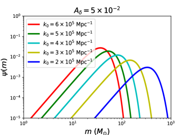
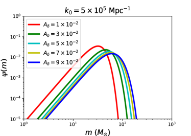
where , and are dimensionless amplitude and constant wave number, respectively. In Fig. 1, we show several examples for the mass function which correspond to the -function power spectrum of primordial curvature perturbation as Eq. (25). Specifically, we choose the constant wave number to be with fixed dimensionless amplitude presented in the left panel of Fig. 1. Similarly, we show the mass function with different dimensionless amplitude and fixed constant wave number presented in the right panel of Fig. 1.
The second case is a nearly scale invariant shape of the form
| (26) |
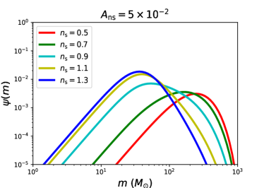
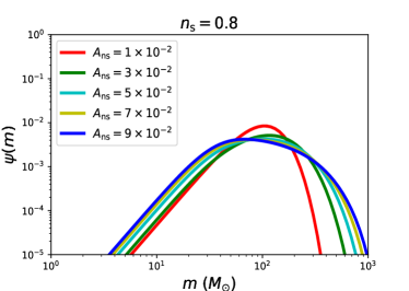
where , and are dimensionless amplitude and spectral tilt, respectively. In addition, We take and as and , which approximately correspond to PBH mass in the range of to . In Fig. 2, we show several examples for the mass function which correspond to the nearly scale invariant power spectrum of primordial curvature perturbation as Eq. (26). The same as the first case, we choose the spectral tilt with fixed dimensionless amplitude presented in the left panel of Fig. 2. Similarly, we show the mass function with different dimensionless amplitude and fixed spectral tilt presented in the right panel of Fig. 2.
In order to discuss the constraints on the power spectrum of primordial curvature perturbation from the lensing effect, we take FRBs as an example. At present, we use publicly available FRBs compiled by zhou et al. 2022 works (Zhou et al., 2022b). These sources consist of more than five hundred FRB events from 2018 July 25 to 2019 July 1111https://www.chime-frb.ca/catalog (CHIME/FRB Collaboration,, 2021). The distance and redshift of a detected FRB can be approximately estimated from its observed dispersion measure (DM), which is proportional to the number density of free electron along the line of sight and is usually decomposed into the following four ingredients,
| (27) |
where and represent DM from host galaxy and local environment, respectively. We adopt the minimum inference of redshift for all host galaxies, which corresponds to the maximum value of to be 200 . is the contribution from the Milky Way. In addition, represents DM contribution from intergalactic medium (IGM). The relation is given by (Deng & Zhang, 2014) and it is approximately expressed as by considering the fraction of baryon in the IGM to and the He ionization history (Zhang, 2018). DM and redshift measurements for several localized FRBs suggested that this relation is statistically favored by observations (Li et al., 2020). We present the inferred redshifts of available FRBs in the left panel of Fig. 3. For milli-lensing of FRBs, the critical value and the width () of the observed signal determine the maximum and minimum value of impact parameter in the cross section. To ensure that both signals are detectable, the maximum value of impact parameter can be obtained by requiring that the flux ratio of two lensed images is smaller than a critical value ,
| (28) |
Here, following previous works Muñoz et al. (2016); Zhou et al. (2022b, a); Oguri et al. (2022); Liao et al. (2020b), we take for cases when we study lensing of the whole sample of all currently public FRBs. In addition, the minimum value of impact parameter can be obtained from the time delay between lensed signals
| (29) |
and pulse widths of all FRBs are presented in the left panel of Fig. 3.
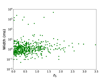
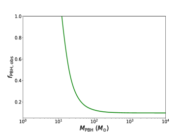
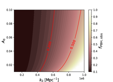
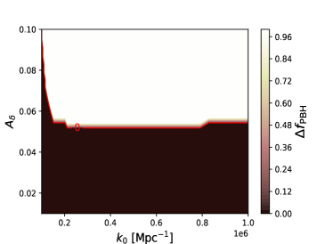
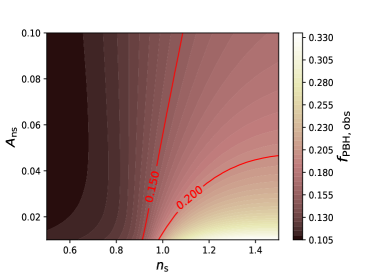
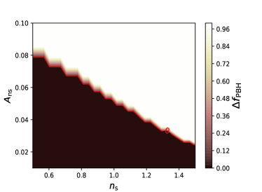
After determining the the maximum and minimum value of impact parameter in the optical depth from Eqs. (28-29), we can combined 593 FRBs and Eq. (15) to obtain the upper limit of at confidence level. In the right panel of Fig. 3, we demonstrate the constraints on when the MMD is considered. In the large-mass end, the constraint on saturates to at 68% confidence level. Then, From the relationship in Eq. (24), we derive the upper limit on corresponding to above two primordial curvature perturbation models, and the results are shown in the left panel of Figs. (4-5). For the first primordial curvature perturbation, we vary the constant wave number from to , which roughly correspond to PBHs with . And, the dimensionless amplitude is greater than 0.01. The regions where and of have been marked by the red solid lines in the left panel of Fig. 4. In addition, it should be note that the white regions in the left panel of Fig. 4 represent that is more than 1. In this model, less and larger corresponds to the smaller peak of the mass distribution function, which leads to improve the constraints on the . In the right panel of Fig. 4, the parameter space can be allowed to exist in the brown area within the red solid line. There are two conditions under which a parameter space can be allowed to exist:
| (30) |
The first condition means that the density parameter of PBH from theory can not be larger than the one of dark matter. The second condition means that the theoretical prediction of PBH abundance should be lower than the upper limit of observational constraints. We find that the amplitude of primordial curvature perturbation is less than at the scale region of .
For the second case, we assume that the value of varies from 0.5 to 1.5 and is greater than 0.01. The regions where and of dark matter can consist of PBHs are denoted by red solid line in the left panel of Fig. 5. In this model, less corresponds to the lagrer peak of the mass distribution function. In addition, larger corresponds to the broader mass distribution. The quantitative competition between the two above-mentioned effects of broadening the mass distribution, hence the constraints on the is more complicated. Based on the above conditions of Eq. (30), we present the allowed parameter space in the brown area within the red solid line at the right panel of Fig. 5. We find that the amplitude of primordial curvature perturbation is less than at the scale invariant range ().
5 Discussion
Although CMB and LSS observations have yielded strict bounds on the primordial curvature perturbation at scale and higher, effective constraints on primordial fluctuations on the small scales are still rare. Fortunately, the gravitational lensing effects, such as echoes of transient sources, can be used as powerful probes to constrain PBHs. Therefore, we proposed using lensing effect to constrain the primordial curvature perturbation on small scales. In this paper, we first derive the relationship that connects constraints of from the MMD to EMD for all lensing effect. Then, taking FRB as an example, we propose that its lensing effect can be used to exploring the primordial curvature perturbation. By combining 593 FRB samples (Zhou et al., 2022b) and two kinds of primordial curvature perturbation models, we present the constraints on and the allowed regions of parameter space of primordial curvature perturbations in Figs. (4-5). In general, null search result of lensed FRB in the latest 593 events would constrain the amplitude of primordial curvature perturbation to be less than at the scale region of . Moreover, there are two significant aspects in our analysis:
-
•
When comparing the abundance of PBHs calculated by any theoretical model with the observational constraints, we should transform the results from MMD to the EMD under the corresponding theoretical framework. For observational constraints from the lensing effect, we can use Eqs. (24) to translate MMD and EMD results.
-
•
Since the primordial power spectrum determines the mass distribution () and theoretical abundance of PBHs (), it suggests that the primordial curvature perturbation parameters are degenerate with the abundance of PBHs theoretically. Therefore, if there is a tension between the predicted range of and from the future lensing signals, we should consider the following possible reasons: 1. Whether the primordial perturbation model is correct; 2. Whether there are other compact dark matter, such as axion mini-clusters (Hardy, 2017) and compact mini halos (Ricotti, 2009), participating in the observation process; 3. Whether PBHs exist evolutionary processes, such as accretion (Ricotti, 2007) and halo structure (Delos & Franciolini, 2023), to change the theoretical or observed physical processes.
There are several factors contributing to the uncertainties in our analysis. For example, the values for depends on the profile of perturbations, the threshold value of the comoving density could vary from 0.2 to 0.6 (Musco & Miller, 2013; Harada et al., 2013; Yoo et al., 2018; Musco et al., 2021). Moreover, non-Gaussian due to the nonlinear relationship between curvature and density perturbations would lead to the amplitude of the power spectrum of primordial curvature perturbation might be a factor of larger than if we assumed a linear relationship between and (Gow et al., 2021; De Luca et al., 2019; Young et al., 2019). Finally, our analysis are based on the Press-Schechter theory. It should be noted that the statistical methods, e.g., Press-Schechter or peaks theory, would slightly affect the results (Gow et al., 2021). It is foreseen that these constraints will be of great importance for exploring PBHs with their formation mechanisms relating to the physics of the early universe.
6 Acknowledgements
This work was supported by the National Key Research and Development Program of China Grant No. 2021YFC2203001; National Natural Science Foundation of China under Grants Nos.11920101003, 12021003, 11633001, 12322301, and 12275021; the Strategic Priority Research Program of the Chinese Academy of Sciences, Grant Nos. XDB2300000 and the Interdiscipline Research Funds of Beijing Normal University. H.Z is supported by China National Postdoctoral Program for Innovative Talents under Grant No.BX20230271.
References
- Ando et al. (2018) Ando, K., Inomata, K., & Kawasaki, M. 2018, PhRvD, 97, 103528
- Barnacka et al. (2012) Barnacka, A., Glicenstein, J.F., & Moderski, R. 2012, PhRvD, 86, 043001
- Basak et al. (2022) Basak, S., Ganguly, A., Haris, K., Kapadia, S., Mehta, A. K., & Ajith, P. 2022, ApJL, 926, L28
- Blaes & Webster (1992) Blaes, O. M., & Webster, R. L. 1992, ApJl, 391, L63
- Cai et al. (2020) Cai, R.-G., Guo, Z.-K., Liu, J., & Liu, L., 2020, JCAP, 06, 013
- Carr et al. (2016) Carr, B., Kuhnel, F., & Sandstad, M. 2016, PhRvD, 94, 083504
- Carr et al. (2017) Carr, B., Raidal, M., Tenkanen, T., Vaskonen, V., & Veermäe, H. 2017, PhRvD, 96, 023514
- Carr & Hawking (1974) Carr, B. J., & Hawking, S. W. 1974, MNRAS, 168, 399
- Carr (1975) Carr, B. J. 1975, ApJ, 201, 1
- Casadio et al. (2021) Casadio, C., Blinov, D., Readhead, A. C. S., et al. 2021, MNRAS, 507, L6
- Chen & Cai (2019) Chen, C., & Cai, Y.-F. 2019, JCAP, 10, 068
- CHIME/FRB Collaboration, (2021) CHIME/FRB Collaboration. 2021, ApJS, 257, 59
- CHIME/FRB Collaboration, (2022) CHIME/FRB Collaboration, 2022, PhRvD, 106, 043016
- Connor & Ravi (2023) Connor, L., & Ravi, V. 2023, MNRAS, 521, 4024
- Clesse & García-Bellido (2015) Clesse, S., & García-Bellido, J. 2015, PhRvD, 92, 023524
- Delos & Franciolini (2023) Delos, M. S., & Franciolini, G. 2023, PhRvD, 107, 083505
- De Luca et al. (2019) De Luca, V., Franciolini, G., Kehagias, A., Peloso, M., Riotto, A., & Ünal, C. 2019, JCAP, 07, 048
- Deng & Zhang (2014) Deng, W., & Zhang, B. 2014, ApJL, 783, L35
- EROS-2 Collaboration, (2007) EROS-2 Collaboration, 2007, A&A, 469, 387
- Fu et al. (2019) Fu, C.-J., Wu, P.-X., & Yu, H.-W. 2019, PhRvD, 100, 063532
- Green & Kavanagh (2021) Green, A. M., & Kavanagh, B. J. 2021, J.Phys.G, 48, 043001
- Gow et al. (2021) Gow, A. D. , Byrnes, C. T., Cole, P. S., & Young, S. 2021, JCAP, 02, 002
- Griest et al. (2013) Griest, K., Cieplak, A. M., & Lehner, M. J. 2013, PhRvL, 111, 181302
- Harada et al. (2013) Harada, T., Yoo, C.-M., & Kohri, K. 2013, PhRvD, 88, 084051
- Hardy (2017) Hardy, E. 2017, JHEP 02, 046
- Hawking (1971) Hawking, S. W. 1971, MNRAS, 152, 75.
- Ji et al. (2018) Ji, L.-Y., Kovetz, E. D., & Kamionkowski, M. 2018, PhRvD, 98, 123523
- Jung & Shin (2019) Jung S., & Shin C. S. 2019, PhRvL, 122, 041103
- Kalita et al. (2023) Kalita, S., Bhatporia, S., & Weltman, A. 2023, JCAP, 11, 059
- Kassiola et al. (1991) Kassiola, A., Kovner, I., & Blandford, B. D. 1991, ApJ, 381, 6
- Krochek & Kovetz (2022) Krochek, K., & Kovetz, E. D. 2022, PhRvD, 10, 103528
- Laha (2020) Laha, R. 2020, PhRvD, 102, 023016
- Leung et al. (2022) Leung, C., Kader, Z., Masui, K. W., et al. 2022, PhRvD 106, 043017
- Li et al. (2020) Li, Z.-X, Gao, H., Wei, J.-J., Yang, Y.-P., Zhang, B., & Zhu, Z.-H. 2020, MNRAS, 496, L28
- Liao et al. (2020a) Liao, K., Tian, S.-X., & Ding, X.-H. 2020a, MNRAS, 495, 2002
- Liao et al. (2020b) Liao, K., Zhang, S.-B., Li, Z.-X, & Gao, H. 2020b, ApJL, 896, L11
- Liao et al. (2022) Liao, K., Biesiada, M., & ,Zhu, Z.-H. 2022, Chin.Phys.Lett., 39, 119801
- LIGO Scientific and VIRGO and KAGRA Collaborations, (2023) LIGO Scientific and VIRGO and KAGRA Collaborations, 2023, arXiv: 2304.08393
- Lin et al. (2022) Lin, S.-J., Li, A., Gao, H., et al. 2022, ApJ, 931, 1
- MACHO Collaboration, (2001) MACHO Collaboration, 2001, ApJL, 550, L169
- Motohashi et al. (2020) Motohashi, H., Mukohyama, S., & Oliosi, M. 2020, JCAP, 03, 002
- Muñoz et al. (2016) Muñoz, J. B., Kovetz E. D., Dai L., & Kamionkowski M. 2016, PhRvL, 117, 091301
- Musco & Miller (2013) Musco, I., & Miller, J. C. 2013, Class.Quant.Grav., 30, 145009
- Musco et al. (2021) Musco, I., De Luca, V., Franciolini, V., & Riotto, A. 2021, PhRvD, 103, 063538
- Nakama et al. (2017) Nakama, T., Silk, J., & Kamionkowski, M. 2017, PhRvD, 95, 043511
- Nemiroff et al. (2001) Nemiroff, R. J., Marani, G. F., Norris, J. P., & Bonnell, J. T. 2001, PhRvL, 86, 580
- Niikura et al. (2019a) Niikura, H., Masahiro, T., Naoki, Y., et al. 2019a, Nature Astronomy, 3, 524.
- Niikura et al. (2019b) Niikura, H., Takada, M., Yokoyama, S., Sumi, T., & Masaki, S. 2019b, PhRvD, 99, 083503
- Oguri et al. (2022) Oguri, M., & Takhistov, V., Kohri, K., 2022, Phys.Lett.B, 847, 138276
- Pi et al. (2018) Pi, S., Zhang, Y.-L., Huang, Q.-G., & Sasaki, M. 2018, JCPA, 05, 042
- Planck Collaboration, (2020a) Planck Collaboration. 2020a, A&A, 641, A10
- Planck Collaboration, (2020b) Planck Collaboration. 2020b, A&A, 641, A6
- Press & Gunn (1973) Press, W. H., & Gunn, J. E. 1973, ApJ, 185, 397
- Press & Schechter (1974) Press, W. H., & Schechter, P. 1974, ApJ, 187, 425
- Ricotti (2007) Ricotti, M. 2007, ApJ, 662, 61
- Ricotti (2009) Ricotti, M. 2009, ApJ, 707, 987
- Sasaki et al. (2018) Sasaki, M., Suyama, T., Tanaka1, T., & Yokoyama, S. 2018, Class.Quant.Grav., 35, 063001
- Urrutia & Vaskonen (2021) Urrutia, J., & Vaskonen, V. 2021, MNRAS, 509, 1358
- Urrutia et al. (2023) Urrutia, J., Vaskonen, V., & Veermäe, H. 2023, PhRvD, 108, 023507
- Wang et al. (2021) Wang, J.-S., Herrera-Martín, A., & Hu, Y.-M. 2021, PhRvD, 104, 083515
- Wilkinson et al. (2001) Wilkinson, P. N., Henstock, D. R., Browne, W. A., et al. 2001, PhRvL, 86, 584
- Yoo et al. (2018) Yoo,C.-M., Harada, T., Garriga, J., & Kohri, K. 2018, PTEP, 12, 123E01
- Young et al. (2014) Young, S., Byrnes, C. T., & Sasaki, M. 2014, JCAP, 07, 045
- Young et al. (2019) Young, S., Musco, I., & Byrnes, C. T. 2019, JCAP, 11, 012
- Zhang (2018) Zhang, B. 2018, ApJL, 867, L21
- Zhou et al. (2022a) Zhou, H., Li, Z.-X., Huang, Z.-Q., Gao, H., & Huang, L. 2022a, MNRAS, 511, 1141
- Zhou et al. (2022b) Zhou, H., Li, Z.-X., Liao, K., Niu, C.-H., Gao, H., Huang, Z.-Q., Huang, L., & Zhang, B. 2022b, ApJ, 928, 124
- Zhou et al. (2022c) Zhou, H., Lian, Y.-J., Li, Z.-X, Cao, S., & Huang, Z.-Q. 2022c, MNRAS, 513, 3627
- Zhou et al. (2022d) Zhou, H., Li, Z.-X., Liao, K., & Huang Z.-Q. 2022d, MNRAS, 518, 149
- Zumalacarregui & Seljak (2018) Zumalacarregui, M., & Seljak, U. 2018, PhRvL, 121, 141101