On the Kepler problem on the Heisenberg group

Abstract

We study the nonholonomic motion of a point particle on the Heisenberg group around the fixed “sun” whose potential is given by the fundamental solution of the sub-Laplacian. We find three independent first integrals of the system and show that its bounded trajectories of the system are wound up around certain surfaces of the fourth order.

Keywords: Heisenberg group, Kepler problem, nonholonomic dynamics, almost Poisson bracket, first integral.

2010 Mathematics Subject Classification: 37N05, 53C17, 70F25, 37J60.

1 Introduction

How would a planet move around the Sun on the Heisenberg group? While studying the problem we found that the authors of the paper [MS15] aim to answer this very question. However, a known feature of nonholonomic mechanics (see e. g. [B03]) is that the variatonal problem (control, geodesics, how to move from A to B) and the dynamics problem (how does it move on its own?) are generally not equivalent. Indeed, for instance, in the geodesic problem on the Heisenberg group, to any initial velocity there corresponds a one-parametric family of geodesics. On the other hand the dynamics is uniquely determined by an initial position and a velocity so it can’t be any geodesic (the actual solutions in in this case are what is known in nonholonomic geometry as the “straightest” lines). It seems to us that the problem actually studied in [MS15] is the variatonal one — how to move efficiently on Heisenberg group in the presence of a gravitational field. Here, we aim to solve the dynamics problem instead.

We consider the Heisenberg group with the left-invariant sub-Riemannian metric and a fixed “sun” at the origin. The potential is given by the fundamental solution of the sub-Laplacian — a generalization of the Laplace–Beltrami operator to the sub-Riemannian manifolds. Traditionally, to derive the non-holonomic equations of motion the Lagrange–d’Alembert principle is used. In Section 2 we remind how the equations of motion can be translated to the form that uses the intrinsic structure of nonholonomic distribution. This allows one to use Hamiltonian language best suited for finding integrals of the system. In Section 3 we apply this to study the Kepler problem on the Heisenberg group and find its first integrals. In contrast to the 6-dimensional variational problem which is not Liouville integrable (proved in [SM21]), the dynamics problem is 5-dimensional and turns out to have at least three independent first integrals. This allows us to rather qualitatively describe the geometry of trajectories of the system. In particular, a typical trajectory of the system winds up around the surface of order 4 which we found explicitly. Due to the nonholonomic constraint the surface in the Heisenberg group uniquely defines the trajectory by its starting point. We also describe a few special trajectories.

In relation to our research we note that the Kepler problem on the Riemannian manifolds was studied extensively starting from works of Lobachevsky [L1835] in hyperbolic space and Serret [S1860] on the sphere. The survey of related works in the spaces of constant curvature may be found in [DPM12]. The aforementioned paper [MS15] has a few followups [DS21, SM21] all of which seem to address the variational problem.

2 Motion on sub-Riemannian manifolds

Here we derive the equations of nonholonomic dynamics in the generalized Hamiltonian form, simplified for the case considered. The general form may be found in [B03].

Consider a mechanical system in $\mathbb{R}^{n}$ with $k$ ideal functionally independent nonintegrable constraints linear in velocities. In Lagrangian coordinates $q^{i}$, $\dot{q}^{i}$ these can be given by

$$\sum_{i=1}^{n}a^{j}_{i}(q)\dot{q}^{i}=0,\quad j=1,\ldots,k.$$ (2.1)

Locally the equations (2.1) can be solved to $k$ dependent velocities and represented in the form

$$\dot{q}^{m+j}=\sum_{i=1}^{m}f^{j}_{i}(q)\dot{q}^{i},\quad j=1,\ldots,k,$$ (2.2)

where $m=n-k$ and the velocities $\dot{q}^{1},\ldots,\dot{q}^{m}$ are assumed to be independent.

Recall that for a nonholonomic system with the Lagrangian $L(q,\dot{q},t)$ and the constraints (2.1) the equations of motion are derived using the Lagrange–d’Alembert principle (see, e. g. [B03])

$$\frac{d}{dt}\frac{\partial L}{\partial\dot{q}^{i}}-\frac{\partial L}{\partial q^{i}}=\sum_{j=1}^{k}\lambda_{j}a^{j}_{i},\quad i=1,\ldots,n,$$ (2.3)

where the Lagrange multipliers $\lambda_{j}$ are determined in such a way that the trajectory satisfies constraints (2.1).

It may be useful, especially for problems with the constraints of form (2.2), instead of the Lagrangian coordinates use the ones in the distribution of admissible velocities. Consider the vector fields

$$X_{i}(q)={\partial q_{i}}+\sum_{j=1}^{k}f^{j}_{i}(q){\partial q_{m+j}},\quad i=1,\ldots,m.$$ (2.4)

Then the velocity $\dot{q}$ satisfies the constraints (2.2) iff $\dot{q}=\sum\limits_{i=1}^{m}\dot{q}^{i}X_{i}$. Introduce the momentum 1-form

$$P=\sum_{i=1}^{n}\frac{\partial L}{\partial\dot{q}^{i}}dq^{i}.$$ (2.5)

Then we can describe the dynamics by the following generalization of Euler–Lagrange equations (in what follows we denote the action of 1-form $\tau$ on the vector field $X$ as $\tau\langle X\rangle$).

Proposition 2.1.

The dynamical motion in the system with the Lagrangian $L(q,\dot{q},t)$ and the constraints (2.2) is described by the system of equations

$$\frac{d}{dt}P\langle X_{i}\rangle=X_{i}L, i=1,\ldots,m,$$ (2.6)

$$\dot{q}^{m+j}=\sum_{i=1}^{m}f^{j}_{i}(q)\dot{q}^{i}, j=1,\ldots,k.$$

Proof.

Introduce 1-forms of our constraints

$$\tau^{j}(q)=dq^{m+j}-\sum_{i=1}^{m}f^{j}_{i}(q)\,dq^{i},\qquad j=1,\ldots,k.$$ (2.7)

Then $\tau^{j}\langle X_{i}\rangle=0$ for $i=1,\ldots,m$ and $\tau^{j}\langle\partial q_{m+l}\rangle=\delta^{j}_{l}$ for $l=1,\ldots,k$. The Lagrange–d’Alembert equations (2.3) can be rewritten in our terms as

$$\frac{d}{dt}P\langle{\partial q_{i}}\rangle-dL\langle{\partial q_{i}}\rangle=\sum_{j=1}^{k}\lambda_{j}\tau^{j}\langle{\partial q_{i}}\rangle,\qquad i=1,\ldots,n.$$

Then, since the expression is linear w. r. t. the term in the angle brackets

$$\frac{d}{dt}P\langle X_{i}\rangle-dL\langle X_{i}\rangle=\sum_{j=1}^{k}\lambda_{j}\tau^{j}\langle X_{i}\rangle=0,\qquad i=1,\ldots,m.$$

The sufficiency of the equations (2.2), (2.6) follows from the fact that we can recover Lagrange–d’Alembert equations from them. Indeed, let

$$\lambda_{j}=\frac{d}{dt}P\langle{\partial q_{m+j}}\rangle-dL\langle{\partial q_{m+j}}\rangle=\frac{d}{dt}\frac{\partial L}{\partial\dot{q}^{m+j}}-\frac{\partial L}{\partial q^{m+j}},\quad j=1,\ldots,k.$$

This gives us the equations (2.3) for $i=m+1,\ldots,n$. Then, since $\partial q_{i}=X_{i}-\sum\limits_{j=1}^{k}f^{j}_{i}(q){\partial q_{m+j}}$ for $i=1,\ldots,m$ we have

$$\frac{d}{dt}\frac{\partial L}{\partial\dot{q}^{i}}-\frac{\partial L}{\partial q^{i}}=\frac{d}{dt}P\langle X_{i}\rangle-dL\langle X_{i}\rangle-\sum_{j=1}^{k}f^{j}_{i}\Big{(}\frac{d}{dt}\frac{\partial L}{\partial\dot{q}^{m+j}}-\frac{\partial L}{\partial q^{m+j}}\Big{)}=-\sum_{j=1}^{k}\lambda_{j}f^{j}_{i}.$$

These are the equations (2.3) for $i=1,\ldots,m$. Thus, the system of equations (2.2), (2.6) is equivalent to the one of (2.2), (2.3). ∎

Let $\mathcal{D}$ be the distribution spanned by $X_{1},\ldots,X_{m}$, i. e. $\mathcal{D}_{q}=\mathrm{span}\,\{X_{1}(q),\ldots,X_{m}(q)\}$. One thing to note is that for deriving equations (2.6) for a particular system it is enough to know the Lagrangian only on $\mathcal{D}$, not on the whole $T\mathbb{R}^{n}$, which allows us to immerse the problem in the sub-Riemannian setting.

Recall that the (regular) sub-Riemannian structure on a smooth manifold $M$ is given by the constant rank distribution $\mathcal{D}\subset TM$ (i. e. $\mathcal{D}_{x}\subset T_{x}M$ is a subspace and $\dim\mathcal{D}_{x}$ is independent of $x$) and the sub-Riemannian metric tensor $\langle\cdot,\cdot\rangle$ on $\mathcal{D}$, i. e. $\langle\cdot,\cdot\rangle_{x}$ is a scalar product on $\mathcal{D}_{x}$.

Let us reformulate the problem in Hamiltonian terms. The energy $E(q,\dot{q},t)$ of the system is defined as usual:

$$E=P\langle\dot{q}\rangle-L$$

and satisfies $\frac{d}{dt}E=-\frac{\partial}{\partial t}L$ on trajectories of the system. Note, that the dual basis to the one of vector fields $X_{1},\ldots,X_{m},\partial q_{m+1},\ldots,\partial q_{m+k}$ consists of 1-forms

$$dq^{1},\ldots,dq^{m},\tau^{1},\ldots,\tau^{k}.$$

In particular, $dq^{1},\ldots,dq^{m}$ form the basis of $\mathcal{D}^{*}$. Introduce the momenta $p=\sum\limits_{i=1}^{m}p_{i}\,dq^{i}$ on $\mathcal{D}^{*}$, i. e. $p\langle X_{i}\rangle=p_{i}$, $i=1,\ldots,m$. Assuming that $\dot{q}(p,q,t)\in\mathcal{D}_{q}$ can be determined uniquely from the equation $p\langle\dot{q}\rangle=P\langle\dot{q}\rangle$ let us define the generalized Hamiltonian $H(p,q,t)$ on $\mathcal{D}^{*}$ as

$$H(p,q,t)=p\langle\dot{q}\rangle-L(q,\dot{q},t)=\sum_{i=1}^{m}p_{i}\dot{q}^{i}-L(q,\dot{q},t).$$

For this assumption to take place it is sufficient to require that the restriction of the quadratic form $\frac{\partial^{2}L}{\partial\dot{q}^{i}\partial\dot{q}^{j}}dq^{i}dq^{j}$ on $\mathcal{D}$ is positive definite.

Reformulating the equations (2.6) in terms of $H$ one obtains

Proposition 2.2.

The dynamical motion in the nonholonomic system with the constraints (2.2) and the generalized Hamiltonian $H(p,q,t)$ on $\mathcal{D}^{*}$ is described by the system of equations

$$\dot{q}^{i}=\frac{\partial H}{\partial p_{i}},\quad\dot{p}_{i}=-X_{i}H, i=1,\ldots,m,$$ (2.8)

$$\dot{q}^{m+j}=\sum_{i=1}^{m}f^{j}_{i}(q)\frac{\partial H}{\partial p_{i}}, j=1,\ldots,k.$$

Proof.

Observe that since the bases $X_{1},\ldots,X_{m},\partial q^{m+1},\ldots,\partial^{m+k}$, introduced in (2.4), and $d\dot{q}^{1},\ldots,d\dot{q}^{m},\tau^{1},\ldots,\tau^{k}$, introduced in (2.7), are dual, for a smooth function $f(q)$ we have

$$df=\sum_{i=1}^{m}df\langle X_{i}\rangle\,dq^{i}+\sum_{j=1}^{k}df\langle\partial q^{m+j}\rangle\,\tau^{j}=\sum_{i=1}^{m}X_{i}f\,dq^{i}+\sum_{j=1}^{k}\frac{\partial f}{\partial q^{m+j}}\,\tau^{j}.$$

Then

$$dL=\sum_{i=1}^{m}X_{i}L\,dq^{i}+\sum_{j=1}^{k}\frac{\partial L}{\partial q^{m+j}}\,\tau^{j}+\sum_{i=1}^{n}\frac{\partial L}{\partial\dot{q}^{i}}d\dot{q}^{i}+\frac{\partial L}{\partial t}dt\\ =\sum_{i=1}^{m}X_{i}L\,dq^{i}+\sum_{j=1}^{k}\frac{\partial L}{\partial q^{m+j}}\,\tau^{j}+\sum_{i=1}^{n}P\langle\partial q^{i}\rangle d\dot{q}^{i}+\frac{\partial L}{\partial t}dt.$$

Further, restricting $L$ on $\mathcal{D}\times\mathbb{R}$ with coordinates $q^{1},\ldots,q^{n}$, $\dot{q}^{1},\ldots,\dot{q}^{m}$, $t$, i. e. setting $\dot{q}=\dot{q}^{1}X_{1}+\ldots+\dot{q}^{m}X_{m}$, we obtain

$$dL|_{T\mathcal{D}}=\sum_{i=1}^{m}X_{i}L\,dq^{i}+\sum_{j=1}^{k}\frac{\partial L}{\partial q^{m+j}}\,\tau^{j}+\sum_{i=1}^{m}P\langle X_{i}\rangle d\dot{q}^{i}+\frac{\partial L}{\partial t}dt.$$

Now, for $H=p\langle\dot{q}\rangle-L(q,\dot{q},t)|_{\mathcal{D}}$ with $\dot{q}=\dot{q}(p,q,t)$ we have

$$dH=\sum_{i=1}^{m}\big{(}p_{i}-P\langle X_{i}\rangle\big{)}\,d\dot{q}^{i}+\sum_{i=1}^{m}\dot{q}^{i}\,dp_{i}-\sum_{i=1}^{m}X_{i}L\,dq^{i}-\sum_{j=1}^{k}\frac{\partial L}{\partial q^{m+j}}\,\tau^{j}-\frac{\partial L}{\partial t}dt.$$

If $\dot{q}$ satisfies $p\langle\dot{q}\rangle=P\langle\dot{q}\rangle$ then the first sum vanishes. Finally, since for the function $H(p,q,t)$

$$dH=\sum_{i=1}^{m}\frac{\partial H}{\partial p_{i}}dp_{i}+\sum_{i=1}^{m}X_{i}H\,dq^{i}+\sum_{j=1}^{k}\frac{\partial H}{\partial q^{m+j}}\tau^{j}+\frac{\partial H}{\partial t}dt,$$

the equations (2.8) follow from (2.6). ∎

Observe that for time independent system $H$ is a first integral of (2.8), (2.2). We can define almost Poisson bracket (see e. g. [B03, Section 3.1]) on $\mathcal{D}^{*}$ as

$$\{F,H\}=\sum_{i=1}^{m}\Big{(}\frac{\partial H}{\partial p_{i}}X_{i}F-\frac{\partial F}{\partial p_{i}}X_{i}H\Big{)}.$$

It retains all the properties of Poisson bracket but the Jacobi identity. Nevertheless, since $\dot{F}=\{F,H\}$ it follows that $F$ is an integral of (2.8), (2.2) iff $\{F,H\}\equiv 0$.

3 Motion in a potential field on the Heisenberg group

Recall that the Heisenberg group $\mathbb{H}^{1}=(\mathbb{R}^{3},\cdot,\delta_{\lambda})$ is a homogeneous group with the group operation

$$(x,y,z)\cdot(x^{\prime},y^{\prime},z^{\prime})=\Big{(}x+x^{\prime},y+y^{\prime},z+z^{\prime}+\frac{xy^{\prime}-x^{\prime}y}{2}\Big{)},$$

and the one-parametric family of anisotropic dilatations

$$\delta_{\lambda}(x,y,z)=(\lambda x,\lambda y,\lambda^{2}z),\quad\lambda>0.$$

Its Lie algebra $\mathfrak{h}^{1}$ of left-invariant vector fields has the basis

$$X=\partial_{x}-\frac{y}{2}\partial_{z},\quad Y=\partial_{y}+\frac{x}{2}\partial_{z},\quad Z=[X,Y]=\partial_{z}.$$

The dual basis of left-invariant 1-forms is

$$dx,\quad dy,\quad\tau=dz+\frac{y\,dx-x\,dy}{2}.$$

The horizontal distribution $\mathcal{D}=\mathop{\mathrm{span}}\{X,Y\}\subset T\mathbb{H}^{1}$ is totally nonholonomic. The form $\tau$ is its annihilator. The sub-Riemannian structure on $\mathbb{H}^{1}$ is given by the quadratic form $\langle\cdot,\cdot\rangle$ on $\mathcal{D}$. We choose the one such that $X,Y$ form the orthonormal basis:

$$ds^{2}=dx^{2}+dy^{2}.$$

While this quadratic form is degenerate on $T\mathbb{H}^{1}$ it is positive definite on $\mathcal{D}$. For the mechanical motion with the kinetic energy $T=\frac{1}{2}ds^{2}\langle\dot{q}\rangle=\frac{1}{2}(\dot{x}^{2}+\dot{y}^{2})$ and the potential energy $U=U(x,y,z)$ one has, as usual, the Lagrangian $L=T-U$. By Proposition 2.2 we can translate equations to the Hamiltonian form where the Hamiltonian $H$ on $\mathcal{D}^{*}$ takes the form $H=2T-L=T+U$, i. e.

$$H(x,y,z,p_{X},p_{Y})=\frac{p_{X}^{2}+p_{Y}^{2}}{2}+U(x,y,z).$$

We are interested in the gravitational potential which in $\mathbb{R}^{n}$ is given by a fundamental solution of the Laplacian. The analogue of Laplace–Beltrami operator on the Heisenberg group is the operator $\Delta_{H}=X^{2}+Y^{2}$. Its fundamental solution is found in [F79]:

$$U=-\frac{k}{\rho^{2}},\quad\text{where }\rho(x,y,z)=((x^{2}+y^{2})^{2}+16\*z^{2})^{\frac{1}{4}}$$

and $k>0$ is some constant. Since both the distribution and the potential have a rotational symmetry around $Oz$ it is natural to make the cylindrical coordinate change $x=r\cos\theta,y=r\sin\theta$. The basis of $\mathcal{D}$ may be given by vector fields

$$R =\phantom{-r}\cos\theta\,X+\phantom{r}\sin\theta\,Y=\partial_{r},$$

$$S =-r\sin\theta\,X+r\cos\theta\,Y=\partial_{\theta}+\tfrac{r^{2}}{2}\partial_{z}.$$

Duals to the basis $R,S,\partial_{z}$ are $dr,d\theta,\tau=dz-\frac{r^{2}}{2}d\theta$ and for the momenta we have

$$p_{X}\,dx+p_{Y}\,dy=(p_{X}\cos\theta+p_{Y}\sin\theta)dr+r(p_{Y}\,\cos\theta-p_{X}\,\sin\theta)d\theta=p_{R}\,dr+p_{S}\,d\theta.$$

It follows that $T=\frac{p_{R}^{2}+p_{S}^{2}/r^{2}}{2}$ and the Hamiltonian becomes

$$H(r,\theta,z,p_{R},p_{S})=\frac{p_{R}^{2}+\frac{1}{r^{2}}p_{S}^{2}}{2}-\frac{k}{(r^{4}+16z^{2})^{\frac{1}{2}}}.$$

Since constraints in the new coordinates still have the form (2.2) we may apply Proposition 2.2 to derive the equations of motion:

$$\dot{r} =\frac{\partial H}{\partial p_{R}}=p_{R}, \dot{p}_{R} =-RH=\frac{p_{S}^{2}}{r^{3}}-\frac{2kr^{3}}{(r^{4}+16z^{2})^{\frac{3}{2}}},$$

$$\dot{\theta} =\frac{\partial H}{\partial p_{S}}=\frac{p_{S}}{r^{2}}, \dot{p}_{S} =-SH=-\frac{8kr^{2}z}{(r^{4}+16z^{2})^{\frac{3}{2}}},$$

$$\dot{z} =\frac{r^{2}}{2}\frac{\partial H}{\partial p_{S}}=\frac{p_{S}}{2}.$$ (3.1)

Theorem 3.1.

If $H<0$ the solutions of (3.1) are bounded with $\sqrt{r^{4}+16z^{2}}\leq\frac{k}{|H|}$.

Proof.

This easily follows from the inequality $H+k/\sqrt{r^{4}+16z^{2}}=\frac{p_{R}^{2}+\frac{1}{r^{2}}p_{S}^{2}}{2}\geq 0$. ∎

In what follows we search for the additional first integrals of the system.

Proposition 3.2.

The system (3.1) does not admit any linear in momenta first integrals.

This statement can be checked by straightforward calculations. We skip the details. However, it turns out that there are a few quadratic integrals in addition to the Hamiltonian $H$.

Theorem 3.3.

The system (3.1) admits quadratic in momenta first integrals

$$F_{1} =\phantom{-}\Big{(}p_{R}p_{S}r-2p_{R}^{2}z+\frac{2p_{S}^{2}z}{r^{2}}\Big{)}\cos(2\theta)+\Big{(}\frac{4p_{R}p_{S}z}{r}-p_{S}^{2}+\frac{kr^{2}}{\sqrt{r^{4}+16z^{2}}}\Big{)}\sin(2\theta),$$

$$F_{2} =-\Big{(}p_{R}p_{S}r-2p_{R}^{2}z+\frac{2p_{S}^{2}z}{r^{2}}\Big{)}\sin(2\theta)+\Big{(}\frac{4p_{R}p_{S}z}{r}-p_{S}^{2}+\frac{kr^{2}}{\sqrt{r^{4}+16z^{2}}}\Big{)}\cos(2\theta),$$

$$F_{3} =(2zp_{R}-rp_{S})^{2}+4z^{2}\Big{(}\frac{p_{S}^{2}}{r^{2}}+\frac{2k}{\sqrt{r^{4}+16z^{2}}}\Big{)}.$$

Any three of $H,F_{1},F_{2},F_{3}$ are functionally independent a. e. wherein all of them satisfy the relation

$$F_{1}^{2}+F_{2}^{2}=2HF_{3}+k^{2}.$$ (3.2)

This theorem can be verified by straightforward calculations. The method we used to construct these integrals is described in Appendix A.

Knowing three independent first integrals allows us to derive the equation of the surface (in coordinates $(r,\theta,z)$) in which the trajectories lie. To do that we introduce two more conserved quantities $J\geq 0$ and in the case $J>0$ also $\theta_{0}\in[0,\pi)$ such that

$$F_{1}=J\sin(2\theta_{0}),\quad F_{2}=J\cos(2\theta_{0}).$$

As main parameters we choose $H,F_{3}$ that do not depend on the angle and the phase offset $\theta_{0}$ that captures the rotational symmetry of the problem. Note, that from the definition $F_{3}\geq 0$ since $k>0$, and $2HF_{3}+k^{2}=J^{2}\geq 0$. Therefore we have one general case and two cases that might require special handling:

• The general case $F_{3}>0$, $J>0$. Then $H>-\frac{k^{2}}{2F_{3}}$ and $\theta_{0}\in[0,\pi)$ is defined.

• The minimum energy case $F_{3}>0$, $J=0$. Then $H=H_{\min}=-\frac{k^{2}}{2F_{3}}$, $\theta_{0}$ is undefined.

• The degenerate case $F_{3}=0$. In this case $J=k$, $\theta_{0}\in[0,\pi)$ is defined and $H$ is unbounded.

Theorem 3.4.

All trajectories of the system (3.1) with the fixed values of the first integrals $H,F_{3},\theta_{0}$ lie on the surface which in the general case $F_{3}>0$, $J>0$ satisfies the equation

$$F_{3}=8z^{2}H+k\sqrt{r^{4}+16z^{2}}-\sqrt{k^{2}+2HF_{3}}\,r^{2}\cos\big{(}2(\theta-\theta_{0})\big{)}.$$ (3.3)

In the minimum energy case $F_{3}>0$, $J=0$ the surface becomes an ellipsoid of revolution

$$4k^{2}z^{2}+kF_{3}r^{2}=F_{3}^{2}.$$ (3.4)

In the degenerate case $F_{3}=0$ the surface degenerates to the straight horizontal line passing through the origin

$$z=0,\quad\theta=\theta_{0}\mod\pi.$$ (3.5)

Proof.

Observe, that we can write $F_{3}$ as

$$F_{3}=8z^{2}H+k\sqrt{r^{4}+16z^{2}}-r^{2}\Big{(}-p_{S}^{2}+\frac{4p_{R}p_{S}z}{r}+\frac{kr^{2}}{\sqrt{r^{4}+16z^{2}}}\Big{)}.$$

From the expressions of $F_{1}$ and $F_{2}$ we have

$$\Big{(}-p_{S}^{2}+\frac{4p_{R}p_{S}z}{r}+\frac{kr^{2}}{\sqrt{r^{4}+16z^{2}}}\Big{)}=F_{1}\sin(2\theta)+F_{2}\cos(2\theta).$$

Therefore,

$$F_{3}=8z^{2}H+k\sqrt{r^{4}+16z^{2}}-r^{2}\big{(}F_{1}\sin(2\theta)+F_{2}\cos(2\theta)\big{)}.$$ (3.6)

Let $F_{3}>0$ and $J>0$. We have $F_{1}\sin(2\theta)+F_{2}\cos(2\theta)=J\cos(2(\theta-\theta_{0}))$ and (3.3) follows.

Now, let $F_{3}>0$ and $J=0$. In this case $F_{1}=F_{2}=0$ and the last term in (3.6) vanishes. Since $H=-\frac{k^{2}}{2F_{3}}$ in this case, (3.6) becomes

$$F_{3}^{2}+4k^{2}z^{2}=kF_{3}\sqrt{r^{4}+16z^{2}}.$$

Squaring and simplifying it we obtain

$$(F_{3}^{2}-4k^{2}z^{2})^{2}=k^{2}F_{3}^{2}r^{4}.$$ (3.7)

By Theorem 3.1 for the trajectories of the system $\sqrt{r^{4}+16z^{2}}\leq\frac{k}{|H|}=\frac{2F_{3}}{k}$. Therefore,

$$F_{3}\geq\tfrac{k}{2}\sqrt{r^{4}+16z^{2}}\geq\tfrac{k}{2}\sqrt{16z^{2}}=2kz.$$

Now (3.4) follows if we take the square root of (3.7).

Lastly, $F_{3}=0$ implies $z=0$ and $J=k>0$. The restriction of (3.6) on $z=0$ becomes

$$0=kr^{2}-kr^{2}\cos(2(\theta-\theta_{0})).$$

This gives us either $r=0$ (the origin) or $\theta=\theta_{0}\mod\pi$. ∎

Remark 3.5.

Solving the equation (3.3) for the square root $\sqrt{r^{4}+z^{2}}$ and then squaring it we obtain the following equation

$$k^{2}(r^{4}+16z^{2})=\big{(}F_{3}-8z^{2}H+\sqrt{k^{2}+2HF_{3}}\,r^{2}\cos\big{(}2(\theta-\theta_{0})\big{)}\big{)}^{2},$$

or in Cartesian coordinates

$$k^{2}((x^{2}+y^{2})^{2}+16z^{2})=\big{(}F_{3}-8z^{2}H+\sqrt{k^{2}+2HF_{3}}\,(\cos(2\theta_{0})(x^{2}-y^{2})+2\sin(2\theta_{0})xy)\big{)}^{2}.$$

We see that this is an equation of the fourth order. However, its solution is a branched surface and only one of its branches is the solution to the original equation, i. e. the equation is quadratic in $z^{2}$ but only one of its two roots solves (3.3).

Examples of the surfaces corresponding to the cases $H=0$ and $H<0$ may be seen on Fig. 1. Next we note a few properties of the surfaces obtained.

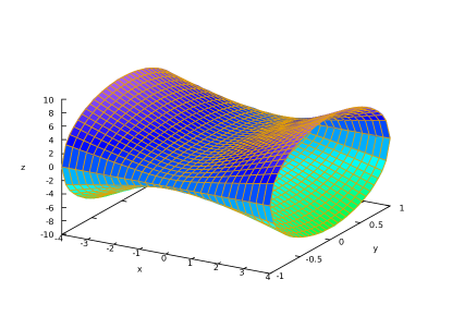
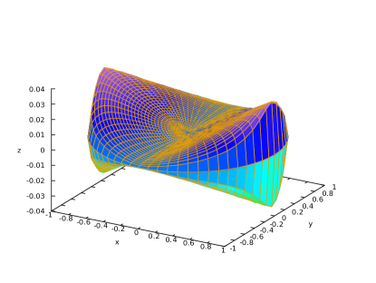
Figure 1: Surfaces corresponding to the cases $H=0$ and $H<0$.

Corollary 3.6.

In the non-degenerate case $F_{3}>0$ the surfaces described in Theorem 3.4 have the following properties.

1. The surface is topologically

   1. a sphere in the case $H<0$;

   2. a cylinder in the case $H\geq 0$.

2. The surface has reflection symmetry in the plane $z=0$ and

   1. in the case $J>0$ it has two more planes of symmetry $\theta=\theta_{0}$ and $\theta=\theta_{0}+\frac{\pi}{2}$;

   2. in the case $J=0$ it is the surface of revolution around $r=0$.

3. The trace of the surface on the plane $z=0$ is a quadratic curve:

   1. in the case $H<0$ it is an ellipse with the semiaxes $\sqrt{\frac{F_{3}}{k-J}}$ and $\sqrt{\frac{F_{3}}{k+J}}$;

   2. in the case $H=0$ it is two parallel lines at the distance $\sqrt{\frac{F_{3}}{k}}$ from the origin;

   3. in the case $H>0$ it is a hyperbola with the semiaxis $\sqrt{\frac{F_{3}}{k+J}}$.

The properties are straightforward and easy to check.

A smooth surface $S\subset\mathbb{H}^{1}$ is transversal to the horizontal distribution $\mathcal{D}$ at almost all points, i. e. $T_{x}S\cap\mathcal{D}_{x}$ is one-dimensional for a. e. $x\in S$. Therefore, the trajectory of the system is rather uniquely defined by a starting point on a surface, with the only possible exception being when the solution arrives at the point tangent to $\mathcal{D}$ with zero velocity. An example of a bounded trajectory ($H<0$) which we belive to be a typical one is presented in Fig. 2. Next we describe special solutions corresponding to the degenerate cases.

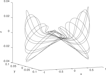
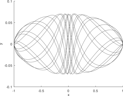
Figure 2: A trajectory and its projection on the plane $Oxy$ with $k=1$ and initial values $x(0)=1$, $y(0)=z(0)=p_{X}(0)=0$, $p_{Y}(0)=\frac{1}{10}$.

Theorem 3.7.

The only trajectories of (3.1) passing through the origin are straight lines in the plane $z=0$. In this case $\theta=const$ and $r(t)$ satisfies the equation $\frac{\dot{r}^{2}}{2}=H+\frac{k}{r^{2}}$. These solutions correspond to the degenerate case $F_{3}=0$.

Proof.

From Corollary 3.6 the trajectories may pass through the origin only in the case $F_{3}=0$, i. e. only if $z\equiv 0$ and $p_{S}\equiv 0$. Then $\dot{\theta}=0$ and the Hamiltonian becomes $H=\frac{\dot{r}^{2}}{2}-\frac{k}{r^{2}}$. ∎

Therefore, the conserved quantity $F_{3}$ serves as a kind of angular/vertical momentum. Two more special solutions appear in the minimal energy case $J=0$.

Theorem 3.8.

The only stationary solutions of (3.1) are points on $Oz$:

$$r=0,\quad z=\pm\frac{k}{4H}.$$

These solutions correspond to the minimal energy case $J=0$.

Proof.

Indeed, outside of the axis $r=0$ the stationary solution must satisfy $p_{S}\equiv 0$. But in this case $\dot{p}_{R}$ is negative and the solution is non-stationary. For the stationary solution on $Oz$ we have $H=-\frac{k}{\sqrt{16z^{2}}}$ and $F_{3}=\frac{8kz^{2}}{\sqrt{16z^{2}}}$. Therefore $J^{2}=k^{2}+2HF_{3}=0$. ∎

Theorem 3.9.

Let $J=0$ and $z_{0}=\frac{k}{4|H|}$. The trajectories of non-stationary solutions to (3.1) are the curves monotone in $z$ and $\theta$ such that being parameterized by $z$ they have the form

$$r(z)=\Big{(}2\frac{z_{0}^{2}-z^{2}}{z_{0}}\Big{)}^{\frac{1}{2}},\qquad\theta(z)=\frac{1}{2}\log\frac{z_{0}+z}{z_{0}-z}+\theta(0),\qquad|z|\leq z_{0}.$$

These solutions connect the stationary points $(0,0,\pm z_{0})$ and take infinite time to approach them, i. e. $t(z)\to\pm\infty$ as $z\to\pm z_{0}$.

Proof.

Note that $F_{3}\geq 0$. Therefore, $J=\sqrt{k^{2}+2HF_{3}}=0$ implies $H<0$. Hence, $H=-\frac{k}{4z_{0}}$ and $F_{3}=-\frac{k^{2}}{2H}=2kz_{0}$. The surface (3.4) in this case is an ellipsoid of revolution

$$\frac{z_{0}r^{2}}{2}+\frac{z^{2}}{z_{0}^{2}}=1.$$

From this equation we find the dependence $r(z)$. Next, from $\frac{d\theta}{dz}=\frac{\dot{\theta}}{\dot{z}}=\frac{2}{r^{2}}$ we also find the expression of $\theta(z)$ in a closed form. This gives us a family of curves described in the statement of the theorem. Take any such curve. From the expression of $H$ we have

$$\frac{\dot{r}^{2}+\frac{4\dot{z}^{2}}{r^{2}}}{2}=\frac{p_{R}^{2}+\frac{p_{S}^{2}}{r^{2}}}{2}=H+\frac{k}{\sqrt{r^{4}+16z^{2}}}=\frac{k(z_{0}^{2}-z^{2})}{4z_{0}(z_{0}^{2}+z^{2})}>0$$ (3.8)

for all points except the poles. Therefore, the velocity along the curve is nonzero except on the endpoints. Hence the solution restricted to a curve is monotone in $z$. From the equation of the surface we have

$$0=z_{0}r\dot{r}+\frac{2z\dot{z}}{z_{0}^{2}}.$$

This together with (3.8) yields the equation on $z$:

$$\dot{z}^{2}=\frac{kz_{0}^{4}(z_{0}^{2}-z^{2})^{2}}{4(z^{2}+z_{0}^{2})(z^{2}+z_{0}^{6})}.$$

Choosing the solution increasing in $z$ we obtain

$$t(z_{1})=\int_{0}^{z_{1}}\frac{dz}{\dot{z}}=\int_{0}^{z_{1}}\frac{2\sqrt{(z^{2}+z_{0}^{2})(z^{2}+z_{0}^{6})}}{\sqrt{k}z_{0}^{2}(z_{0}^{2}-z^{2})}\,dz$$

which diverges as $z_{1}\to\pm z_{0}$. The theorem is proved. ∎

4 Conclusion

In conclusion we see that the variational problem and the dynamics problem on the Heisenberg group are vastly different. While the first is Hamiltonian but non-integrable in Liouville sense, the second one, being non-Hamiltonian has at least three first integrals. Both problems are interesting but provide a different insight into the nonholonomic world.

Acknowledgements: While the problem was mainly considered by the first author he is very grateful to second author for deriving the first integrals (Proposition 3.2, Theorem 3.3 and Appendix) which significantly progressed the research and for overall critical comments.

The images were prepared using GNUPlot and Maxima free software.

Appendix A Derivation of quadratic first integrals

By definition any first integral $F$ of (3.1) must satisfy the following relation:

$$\frac{dF}{dt}=\frac{\partial F}{\partial r}p_{R}+\frac{\partial F}{\partial\theta}\frac{p_{S}}{r^{2}}+\frac{\partial F}{\partial z}\frac{p_{S}}{2}+\frac{\partial F}{\partial p_{R}}\left(\frac{p_{S}^{2}}{r^{3}}-\frac{2kr^{3}}{(r^{4}+16z^{2})^{3/2}}\right)-\frac{\partial F}{\partial p_{S}}\frac{8kr^{2}z}{(r^{4}+16z^{2})^{3/2}}=0.$$ (A.1)

It is quite natural to search for the first integrals of (3.1) having the form of non-homogeneous polynomials in momenta.

We shall search for the quadratic integral of (3.1) in the form:

$$F=a\,p_{R}^{2}+d\,p_{R}p_{S}+b\,p_{S}^{2}+f\,p_{R}+g\,p_{S}+h,$$

where all the coefficients are unknown functions which depend on $r$, $\theta$, $z$. Writing down the condition (A.1) for such an integral $F$, we obtain the system of PDEs which splits into two parts: the first one contains relations between the unknown functions $a$, $b$, $d$, $h$ only, the second one is between $f$ and $g$. As in Proposition 3.2, it is easy to check that if $F$ is the first integral, then both functions $f$ and $g$ must vanish identically. So we start our analysis with an integral of the form

$$F=a(r,\theta,z)p_{R}^{2}+d(r,\theta,z)p_{R}p_{S}+b(r,\theta,z)p_{S}^{2}+h(r,\theta,z).$$

The condition (A.1) implies:

$$a_{r}=0,$$ (A.2)

$$2a_{\theta}+r^{2}(a_{z}+2d_{r})=0,$$ (A.3)

$$4a+r^{3}d_{z}+2r(d_{\theta}+r^{2}b_{r})=0,$$ (A.4)

$$2d+r^{3}b_{z}+2rb_{\theta}=0,$$ (A.5)

$$2r^{3}(r^{4}+16z^{2})^{3/2}h_{r}-8kr^{6}a-16kr^{5}zd=0,$$ (A.6)

$$r(r^{4}+16z^{2})^{3/2}(r^{2}h_{z}+2h_{\theta})-4kr^{6}d-32kr^{5}zb=0.$$ (A.7)

Integrating the equations (A.2)–(A.4) successively, we obtain

$$a(r,\theta,z)=\alpha(\theta,z),\qquad d(r,\theta,z)=\gamma(\theta,z)-\frac{1}{2}r\alpha_{z}+\frac{\alpha_{\theta}}{r},$$

$$b(r,\theta,z)=\frac{\alpha}{r^{2}}+\frac{\alpha_{\theta\theta}}{2r^{2}}+\frac{r^{2}\alpha_{zz}}{8}+\frac{\gamma_{\theta}}{r}-\frac{r\gamma_{z}}{2}+\omega(\theta,z),$$

where $\alpha(\theta,z)$, $\gamma(\theta,z)$, $\omega(\theta,z)$ are arbitrary functions. Then (A.5) takes the form

$$\alpha_{zzz}r^{6}-4\gamma_{zz}r^{5}+(2\alpha_{\theta zz}+8\omega_{z})r^{4}+4(\alpha_{\theta\theta z}+4\omega_{\theta})r^{2}+16(\gamma_{\theta\theta}+\gamma)r+8(\alpha_{\theta\theta\theta}+\alpha_{\theta})=0.$$

This is a polynomial in $r$ with coefficients depending on $\theta$, $z$ only. Since this polynomial must vanish, all its coefficients must vanish as well. This allows one to find $\alpha(\theta,z)$, $\gamma(\theta,z)$, $\omega(\theta,z)$ and, consequently, the coefficients $a(r,\theta,z)$, $b(r,\theta,z)$, $d(r,\theta,z)$ explicitly. We omit these long but simple calculations and skip the final form of these coefficients since they are quite cumbersome.

After that we are left with two equations (A.6), (A.7) on the unknown function $h(r,\theta,z)$ which take the form:

$$(r^{4}+16z^{2})^{3/2}h_{r}+2kr(c_{8}r^{2}-z(4c_{9}+z(4c_{3}+c_{5}r^{2}+4c_{6}z)))\cos(2\theta)$$

$$-2kr(c_{9}r^{2}+z(4c_{8}+z(4c_{2}-c_{6}r^{2}+4c_{5}z)))\sin(2\theta)-4kr^{3}(c_{7}-c_{4}z^{2})$$

$$-8kr^{2}z((s_{2}+s_{4}z)\cos\theta+(s_{3}+s_{5}z)\sin\theta)=0,$$ (A.8)

$$(r^{4}+16z^{2})^{3/2}(r^{2}h_{z}+2h_{\theta})+2c_{1}kr^{2}(r^{4}-16z^{2})$$

$$-kr^{2}(4c_{9}r^{2}+c_{2}(r^{4}+16z^{2})-2z(-8c_{8}+2c_{3}r^{2}+c_{5}r^{4}+6c_{6}r^{2}z-8c_{5}z^{2}))\cos(2\theta)$$

$$+kr^{2}(-4c_{8}r^{2}+c_{3}(r^{4}+16z^{2})+2z(8c_{9}+2c_{2}r^{2}-c_{6}r^{4}+6c_{5}r^{2}z+8c_{6}z^{2}))\sin(2\theta)$$

$$-4kr^{3}(s_{2}r^{2}+z(8s_{3}-3s_{4}r^{2}+8s_{5}z))\cos\theta+4kr^{3}(-s_{3}r^{2}+z(8s_{2}+3s_{5}r^{2}+8s_{4}z))\sin\theta$$

$$-4kr^{2}z(8c_{7}+8s_{1}r^{2}+c_{4}(r^{4}+8z^{2}))=0.$$ (A.9)

Here $c_{k}$, $s_{k}$ are arbitrary constants. The equation (A.8) can be integrated. However, the general solution $h(r,\theta,z)$ to (A.8) is expressed in terms of elliptic integrals. We consider the simplest case

$$s_{2}=s_{3}=s_{4}=s_{5}=0.$$

In this case $h(x,y,z)$ can be found from (A.8) in terms of elementary functions as follows:

$$h(r,\theta,z)=\psi(\theta,z)+\frac{k}{4z\sqrt{r^{4}+16z^{2}}}\phi(r,\theta,z),$$

where $\psi(\theta,z)$ is an arbitrary function and

$$\phi(r,\theta,z)=(c_{9}r^{2}+z(4c_{8}+c_{3}r^{2}+c_{6}r^{2}z-4c_{5}z^{2}))\cos(2\theta)\\ +(c_{8}r^{2}+z(-4c_{9}+c_{2}r^{2}+c_{5}r^{2}z+4c_{6}z^{2}))\sin(2\theta)+8z(c_{4}z^{2}-c_{7}).$$

The unknown function $\psi(\theta,z)$ should be chosen such that the relation (A.9) holds identically. It seems that the only possible way to satisfy this requirement is to put

$$\psi(\theta,z)\equiv 0,\qquad c_{1}=c_{5}=c_{6}=c_{8}=c_{9}=s_{1}=0.$$

In this case (A.9) is satisfied. Thus we found all the coefficients of $F.$ Notice that $\widetilde{F}=4F-8c_{7}H$ is also the first integral of (3.1) having the simpler form:

$$\widetilde{F}=\widetilde{a}\,p_{R}^{2}+\widetilde{d}\,p_{R}p_{S}+\widetilde{b}\,p_{S}^{2}+\widetilde{h},$$

where

$$\widetilde{a} =2z(2c_{4}z-c_{2}\cos(2\theta)+c_{3}\sin(2\theta)),$$

$$\widetilde{d} =\Big{(}c_{2}r+\frac{4c_{3}z}{r}\Big{)}\cos(2\theta)-\Big{(}c_{3}x-\frac{4c_{2}z}{r}\Big{)}\sin(2\theta)-4c_{4}rz,$$

$$\widetilde{b} =\frac{1}{r^{2}}\big{(}(-c_{3}r^{2}+2c_{2}z)\cos(2\theta)-(c_{2}r^{2}+2c_{3}z)\sin(2\theta)+c_{4}(r^{4}+4z^{2})\big{)},$$

$$\widetilde{h} =\frac{k}{\sqrt{r^{4}+16z^{2}}}\big{(}r^{2}(c_{3}\cos(2\theta)+c_{2}\sin(2\theta))+8c_{4}z^{2}\big{)}.$$

Here $c_{2}$, $c_{3}$, $c_{4}$ are arbitrary constants. It is left to notice that $\widetilde{F}$ is linear in these constants, i. e. it has the form $\widetilde{F}=c_{2}F_{1}+c_{3}F_{2}+c_{4}F_{3}$. This implies that the functions

$$F_{1} =\phantom{-}\Big{(}p_{R}p_{S}r-2p_{R}^{2}z+\frac{2p_{S}^{2}z}{r^{2}}\Big{)}\cos(2\theta)+\Big{(}-p_{S}^{2}+\frac{4p_{R}p_{S}z}{r}+\frac{kr^{2}}{\sqrt{r^{4}+16z^{2}}}\Big{)}\sin(2\theta),$$

$$F_{2} =-\Big{(}p_{R}p_{S}r-2p_{R}^{2}z+\frac{2p_{S}^{2}z}{r^{2}}\Big{)}\sin(2\theta)+\Big{(}-p_{S}^{2}+\frac{4p_{R}p_{S}z}{r}+\frac{kr^{2}}{\sqrt{r^{4}+16z^{2}}}\Big{)}\cos(2\theta),$$

$$F_{3} =4z^{2}p_{R}^{2}-4rzp_{R}p_{S}+\frac{r^{4}+4z^{2}}{r^{2}}p_{S}^{2}+\frac{8kz^{2}}{\sqrt{r^{4}+16z^{2}}}.$$

are also integrals of (3.1).

Sergey Basalaev
Novosibirsk State University, 1 Pirogova st., 630090 Novosibirsk Russia
e-mail: s.basalaev@g.nsu.ru

Sergei Agapov
Sobolev Institute of Mathematics, 4 Acad. Koptyug avenue, 630090 Novosibirsk Russia
e-mail: agapov@math.nsc.ru, agapov.sergey.v@gmail.com

References

• [B03] A. M. Bloch et al., Nonholonomic Mechanics and Control / Interdisciplinary Applied Math. 24 (2003), 501 pp.
• [DPM12] F. Diacu, E. Pérez-Chavela, M. Santoprete, The $n$-body Problem in Spaces of Constant Curvature. Part I: Relative Equilibria // J. Nonlinear Sci. 22 (2012), 247–266, DOI: 10.1007/s00332-011-9116-z
• [DS21] V. Dods, C. Shanbrom, Self-similarity in the Kepler–Heisenberg Problem // J. Nonlinear Sci. 31 (2021), Article 49, DOI: 10.1007/s00332-021-09709-1
• [F79] G. Folland, A fundamental solution for a subellipic operator // Bulletin of the AMS 79:2 (1973), 373–376.
• [L1835] N. I. Lobachevsky, The new foundations of geometry with full theory of parallels / Collected Works 1835–1838 2, GITTL, Moscow, 1949, 159 pp. [in Russian]
• [MS15] R. Montgomery, C. Shanbrom, Keplerian Dynamics on the Heisenberg Group and Elsewhere // Fields Inst. Commun. 73 (2015), 319–342, arXiv:1212.2713 [math.DS]
• [S1860] P. J. Serret Théorie nouvelle géométrique et mécanique des lignes a double courbre / Librave de Mallet-Bachelier, Paris, 1860.
• [SM21] T. Stachowiak, A. J. Maciejewski, Non-Integrability of the Kepler and the Two-Body Problems on the Heisenberg Group // SIGMA 17 (2021), Article 074, arXiv:2103.10495 [math-ph], DOI: 10.3842/SIGMA.2021.074