SAM-6D: Segment Anything Model Meets Zero-Shot 6D Object Pose Estimation

Abstract

Zero-shot 6D object pose estimation involves the detection of novel objects with their 6D poses in cluttered scenes, presenting significant challenges for model generalizability. Fortunately, the recent Segment Anything Model (SAM) has showcased remarkable zero-shot transfer performance, which provides a promising solution to tackle this task. Motivated by this, we introduce SAM-6D, a novel framework designed to realize the task through two steps, including instance segmentation and pose estimation. Given the target objects, SAM-6D employs two dedicated sub-networks, namely Instance Segmentation Model (ISM) and Pose Estimation Model (PEM), to perform these steps on cluttered RGB-D images. ISM takes SAM as an advanced starting point to generate all possible object proposals and selectively preserves valid ones through meticulously crafted object matching scores in terms of semantics, appearance and geometry. By treating pose estimation as a partial-to-partial point matching problem, PEM performs a two-stage point matching process featuring a novel design of background tokens to construct dense 3D-3D correspondence, ultimately yielding the pose estimates. Without bells and whistles, SAM-6D outperforms the existing methods on the seven core datasets of the BOP Benchmark for both instance segmentation and pose estimation of novel objects.

Figure 1: We present SAM-6D for zero-shot 6D object pose estimation. SAM-6D takes an RGB image (a) and a depth map (b) of a cluttered scene as inputs, and performs instance segmentation (d) and pose estimation (e) for novel objects (c). We present the qualitative results of SAM-6D on the seven core datasets of the BOP benchmark [50], including YCB-V, LM-O, HB, T-LESS, IC-BIN, ITODD and TUD-L, arranged from left to right. Best view in the electronic version.

1 Introduction

Object pose estimation is fundamental in many real-world applications, such as robotic manipulation and augmented reality. Its evolution has been significantly influenced by the emergence of deep learning models. The most studied task in this field is Instance-level 6D Pose Estimation [59, 54, 56, 48, 18, 19], which demands annotated training images of the target objects, thereby making the deep models object-specific. Recently, the research emphasis gradually shifts towards the task of Category-level 6D Pose Estimation [57, 52, 28, 27, 29, 7, 30] for handling unseen objects, yet provided they belong to certain categories of interest. In this paper, we thus delve into a broader task setting of Zero-shot 6D Object Pose Estimation [26, 5], which aspires to detect all instances of novel objects, unseen during training, and estimate their 6D poses. Despite its significance, this zero-shot setting presents considerable challenges in both object detection and pose estimation.

Recently, Segment Anything Model (SAM) [25] has garnered attention due to its remarkable zero-shot segmentation performance, which enables prompt segmentation with a variety of prompts, e.g., points, boxes, texts or masks. By prompting SAM with evenly sampled 2D grid points, one can generate potential class-agnostic object proposals, which may be highly beneficial for zero-shot 6D object pose estimation. To this end, we propose a novel framework, named SAM-6D, which employs SAM as an advanced starting point for the focused zero-shot task. Fig. 2 gives an overview illustration of SAM-6D. Specifically, SAM-6D employs an Instance Segmentation Model (ISM) to realize instance segmentation of novel objects by enhancing SAM with a carefully crafted object matching score, and a Pose Estimation Model (PEM) to solve object poses through a two-stage process of partial-to-partial point matching.

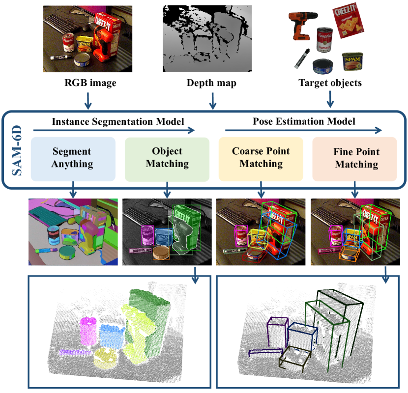
Figure 2: An overview of our proposed SAM-6D, which consists of an Instance Segmentation Model (ISM) and a Pose Estimation Model (PEM) for joint instance segmentation and pose estimation of novel objects in RGB-D images. ISM leverages the Segment Anything Model (SAM) [25] to generate all possible proposals and selectively retains valid ones based on object matching scores. PEM involves two stages of point matching, from coarse to fine, to establish 3D-3D correspondence and calculate object poses for all valid proposals. Best view in the electronic version.

The Instance Segmentation Model (ISM) is developed using SAM to take advantage of its zero-shot abilities for generating all possible class-agnostic proposals, and then assigns a meticulously calculated object matching score to each proposal for ascertaining whether it aligns with a given novel object. In contrast to methods that solely focus on object semantics [38, 5], we design the object matching scores considering three terms, including semantics, appearance and geometry. For each proposal, the first term assesses its semantic matching degree to the rendered templates of the object, while the second one further evaluates its appearance similarities to the best-matched template. The final term considers the matching degree based on geometry, such as object shape and size, by calculating the Intersection-over-Union (IoU) value between the bounding boxes of the proposal and the 2D projection of the object transformed by a rough pose estimate.

The Pose Estimation Model (PEM) is designed to calculate a 6D object pose for each identified proposal that matches the given novel object. Initially, we formulate this pose estimation challenge as a partial-to-partial point matching problem between the sampled point sets of the proposal and the target object, considering the factors such as occlusions, segmentation inaccuracies, and sensor noises. To solve this problem, we propose a simple yet effective solution that involves the use of background tokens. Specifically, for the two point sets, we learn to align their non-overlapping points with the background tokens in the feature space, and thus effectively establish an assignment matrix between them to build the necessary correspondence for predicting the object pose. Based on the design of background tokens, we further develop PEM with two point matching stages, i.e., Coarse Point Matching and Fine Point Matching. The first stage realizes sparse correspondence to derive an initial object pose, which is subsequently used to transform the point set of the proposal, enabling the learning of positional encodings. The second stage incorporates the positional encodings of the two point sets to inject the initial correspondence, and builds dense correspondence for estimating a more precise object pose. To effectively model the dense interactions in the second stage, we propose an innovative design of Sparse-to-Dense Point Transformers, which realize interactions on the sparse versions of the dense features, and subsequently, distribute the enhanced sparse features back to the dense ones using Linear Transformers [23, 12].

For the two models of SAM-6D, ISM, built on SAM, does not require any network re-training or fine-tuning, while PEM is trained on the large-scale synthetic images of ShapeNet-Objects [4] and Google-Scanned-Objects [9] datasets provided by [26]. We evaluate SAM-6D on the seven core datasets of the BOP benchmark [50], including LM-O, T-LESS, TUD-L, IC-BIN, ITODD, HB, and YCB-V. The qualitative results are visualized in Fig. 1. SAM-6D outperforms the existing methods on both tasks of instance segmentation and pose estimation of novel objects, thereby showcasing its robust generalization capabilities.

Our main contributions could be summarized as follows:

• We propose a novel framework of SAM-6D, which realizes joint instance segmentation and pose estimation of novel objects from RGB-D images, and outperforms the existing methods on the seven core datasets of the BOP benchmark.

• We leverage the zero-shot capacities of Segmentation Anything Model to generate all possible proposals, and devise a novel object matching score to identify the proposals corresponding to novel objects.

• We approach pose estimation as a partial-to-partial point matching problem with a simple design of background tokens, and propose a two-stage point matching model for pose estimation of novel objects. The first stage realizes coarse point matching to derive initial object poses, which are then refined in the second stage of fine point matching using Sparse-to-Dense Point Transformers.

2 Related Work

2.1 Segment Anything

Segment Anything (SA), introduced in [25], is a promptable segmentation task that focuses on predicting valid masks for various types of prompts, e.g., points, boxes, text, and masks. To tackle this task, the authors propose a powerful segmentation model called Segment Anything Model (SAM), which comprises three components, including an image encoder, a prompt encoder and a mask decoder. SAM has demonstrated remarkable zero-shot transfer segmentation performance in real-world scenarios, including challenging situations such as medical images [35, 34], camouflaged objects [51, 21], and transparent objects [13, 22]. Moreover, SAM has exhibited high versatility across numerous vision applications [65], such as 2D image inpainting [58, 60, 63, 33], object tracking [15, 61, 68], 3D detection and segmentation [66, 62, 2], and 3D reconstruction [46, 55, 3].

Recent studies have also investigated semantically segmenting anything due to the critical role of semantics in vision tasks. Semantic Segment Anything (SSA) [6] is proposed on top of SAM, aiming to assign semantic categories to the masks generated by SAM. Both PerSAM [67] and Matcher [32] employ SAM to segment the object belonging to a specific category in a query image by searching for point prompts with the aid of a reference image containing an object of the same category. CNOS [38] is proposed to segment all instances of a given object model, which firstly generates mask proposals via SAM and subsequently filters out proposals with low feature similarities against object templates rendered from the object model.

To improve the efficiency of SAM, FastSAM [69] is proposed, which utilizes instance segmentation networks with regular convolutional networks instead of visual transformers used in SAM. Additionally, MobileSAM [64] replaces the heavy encoder of SAM with a lightweight one through decoupled distillation.

2.2 Pose Estimation of Novel Objects

Methods Based on Image Matching Methods within this group [39, 31, 1, 47, 36, 43, 37, 26] often involve comparing object proposals to templates of the given novel objects, which are rendered with a series of object poses, to retrieve the best-matched object poses. For example, both Gen6D [31] and OVE6D [1] are designed to select the viewpoint rotations via image matching and then estimate the in-plane rotations to obtain the final estimates. MegaPose [26] employs a coarse estimator to treat image matching as a classification problem, of which the recognized object poses are further updated by a refiner.

Methods Based on Feature Matching Methods within this group [20, 11, 49, 17, 10, 5] learn to align the 2D pixels or 3D points of the object proposals with the surface points of the given novel objects in the feature space, thereby building 2D-3D or 3D-3D correspondence to compute the object poses. OnePose [49] matches the pixel descriptors of proposals with the aggregated point descriptors of the point sets constructed by Structure from Motion (SfM) for 2D-3D correspondence, while OnePose++ [17] further improves it with a keypoint-free SfM and a sparse-to-dense 2D-3D matching network. ZeroPose [5] is proposed to realize 3D-3D matching based on geometric structures of the proposals and target objects. Moreover, [11] introduces a zero-shot category-level 6D pose estimation task, along with a self-supervised semantic correspondence learning method.

3 Methodology of SAM-6D

We present SAM-6D for zero-shot 6D object pose estimation, which aims to detect all instances of a specific novel object, unseen during training, along with their 6D object poses in the RGB-D images. To realize the challenging task, SAM-6D breaks it down into two steps via two dedicated sub-networks, i.e., an Instance Segmentation Model (ISM) and a Pose Estimation Model (PEM), to first segment all instances and then individually predict their 6D poses, as shown in Fig. 2. We detail the architectures of ISM and PEM in Sec. 3.1 and Sec. 3.2, respectively.

3.1 Instance Segmentation Model

SAM-6D uses an Instance Segmentation Model (ISM) to segment the instances of a novel object $\mathcal{O}$. Given a cluttered scene, represented by an RGB image $\mathcal{I}$, ISM leverages the zero-shot transfer capabilities of Segment Anything Model (SAM) [25] to generate all possible proposals $\mathcal{M}$. For each proposal $m\in\mathcal{M}$, ISM calculates an object matching score $s_{m}$ to assess the matching degree between $m$ and $\mathcal{O}$ in terms of semantics, appearance, and geometry. The matched instances with $\mathcal{O}$ can then be identified by simply setting a matching threshold $\delta_{m}$.

In this subsection, we initially provide a brief review of SAM in Sec. 3.1.1 and then explain the computation of the object matching score $s_{m}$ in Sec. 3.1.2.

3.1.1 Preliminaries of Segment Anything Model

Given an RGB image $\mathcal{I}$, Segment Anything Model (SAM) [25] realizes promptable segmentation with various types of prompts $\mathcal{P}_{r}$, e.g., points, boxes, texts, or masks. Specifically, SAM consists of three modules, including an image encoder $\Phi_{\text{Image}}$, a prompt encoder $\Phi_{\text{Prompt}}$, and a mask decoder $\Psi_{\text{Mask}}$, which could be formulated as follows:

$$\mathcal{M},\mathcal{C}=\Psi_{\text{Mask}}(\Phi_{\text{Image}}(I),\Phi_{\text{Prompt}}(\mathcal{P}_{r})),$$ (1)

where $\mathcal{M}$ and $\mathcal{C}$ denote the predicted proposals and the corresponding confidence scores, respectively.

To realize zero-shot transfer, one can prompt SAM with evenly sampled 2D grids to yield all possible proposals, which can then be filtered based on confidence scores, retaining only those with higher scores, and applied to Non-Maximum Suppression to eliminate redundant detections.

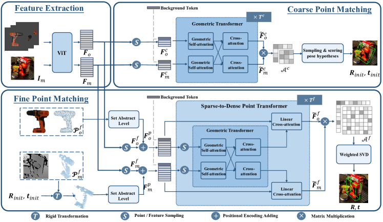
Figure 3: An illustration of Pose Estimation Model (PEM) of SAM-6D.

3.1.2 Object Matching Score

Given the proposals $\mathcal{M}$, the next step is to identify the ones that are matched with a specified object $\mathcal{O}$ by assigning each proposal $m\in\mathcal{M}$ with an object matching score $s_{m}$, which comprises three terms, each evaluating the matches in terms of semantics, appearance, and geometry, respectively.

Following [38], we sample $N_{\mathcal{T}}$ object poses in SE(3) space to render the templates $\{\mathcal{T}_{k}\}_{k=1}^{N_{\mathcal{T}}}$ of $\mathcal{O}$, which are fed into a pretrained visual transformer (ViT) backbone [8] of DINOv2 [42], resulting in the class embedding $\bm{f}^{cls}_{\mathcal{T}_{k}}$ and $N^{patch}_{\mathcal{T}_{k}}$ patch embeddings $\{\bm{f}^{patch}_{\mathcal{T}_{k},i}\}_{i=1}^{N^{patch}_{\mathcal{T}_{k}}}$ of each template $\mathcal{T}_{k}$. For each proposal $m$, we crop the detected region out from $\mathcal{I}$, and resize it to a fixed resolution. The image crop is denoted as $\mathcal{I}_{m}$ and it is also processed through the same ViT to obtain the class embedding $\bm{f}^{cls}_{\mathcal{I}_{m}}$ and the patch embeddings $\{\bm{f}^{patch}_{\mathcal{I}_{m},j}\}_{j=1}^{N^{patch}_{\mathcal{I}_{m}}}$, with $N^{patch}_{\mathcal{I}_{m}}$ denoting the number of patches within the object mask. Subsequently, we calculate the values of the individual scores.

Semantic Matching Score We compute a semantic score $s_{sem}$ through the class embeddings by averaging the top K values from $\{\frac{<\bm{f}^{cls}_{\mathcal{I}_{m}},\bm{f}^{cls}_{\mathcal{T}_{k}}>}{|\bm{f}^{cls}_{\mathcal{I}_{m}}|\cdot|\bm{f}^{cls}_{\mathcal{T}_{k}}|}\}_{i=1}^{N_{\mathcal{T}}}$ to establish a robust measure of semantic matching, with $<,>$ denoting an inner product. The template that yields the highest semantic value can be seen as the best-matched template, denoted as $\mathcal{T}_{best}$, and is used in the computation of the subsequent two scores.

Appearance Matching Score Given $\mathcal{T}_{best}$, we compare $\mathcal{I}_{m}$ and $\mathcal{T}_{best}$ in terms of appearance using a appearance score $s_{appe}$, based on the patch embeddings, as follows:

$$s_{appe}=\frac{1}{N^{patch}_{\mathcal{I}_{m}}}\sum_{j=1}^{N^{patch}_{\mathcal{I}_{m}}}\max_{i=1,\dots,N^{patch}_{\mathcal{T}_{best}}}\frac{<\bm{f}^{patch}_{\mathcal{I}_{m},j},\bm{f}^{patch}_{\mathcal{T}_{best},i}>}{|\bm{f}^{patch}_{\mathcal{I}_{m},j}|\cdot|\bm{f}^{patch}_{\mathcal{T}_{best},i}|}.$$ (2)

$s_{appe}$ is utilized to distinguish objects that are semantically similar but differ in appearance.

Geometric Matching Score In terms of geometry, we score the proposal $m$ by considering factors like object shapes and sizes. Utilizing the object rotation from $\mathcal{T}_{best}$ and the mean location of the cropped points of $m$, we have a coarse pose to transform the object $\mathcal{O}$, which is then projected onto the image to obtain a compact bounding box $\mathcal{B}_{o}$. Afterwards, the Intersection-over-Union (IoU) value between $\mathcal{B}_{o}$ and the bounding box $\mathcal{B}_{m}$ of $m$ is used as the geometric score $s_{geo}$:

$$s_{geo}=\frac{\mathcal{B}_{m}\bigcap\mathcal{B}_{o}}{\mathcal{B}_{m}\bigcup\mathcal{B}_{o}}.$$ (3)

The reliability of $s_{geo}$ is easily impacted by occlusions. We thus compute a visible ratio $r_{vis}$ to evaluate the confidence of $s_{geo}$, which is detailed in the supplementary materials.

By combining the above three score terms, the object matching score $s_{m}$ could be formulated as follows:

$$s_{m}=\frac{s_{sem}+s_{appe}+r_{vis}\cdot s_{geo}}{2+r_{vis}}.$$ (4)

3.2 Pose Estimation Model

SAM-6D uses a Pose Estimation Model (PEM) to predict the 6D poses of the proposals matched with the object $\mathcal{O}$.

For each object proposal $m$, PEM uses a strategy of point registration to predict the 6D pose w.r.t. $\mathcal{O}$. Denoting the sampled point set of $m$ as $\mathcal{P}_{m}\in\mathbb{R}^{N_{m}\times 3}$ with $N_{m}$ points and that of $\mathcal{O}$ as $\mathcal{P}_{o}\in\mathbb{R}^{N_{o}\times 3}$ with $N_{o}$ points, the goal is to solve an assignment matrix to present the partial-to-partial correspondence between $\mathcal{P}_{m}$ and $\mathcal{P}_{o}$. Partial-to-partial correspondence arises as $\mathcal{P}_{o}$ only partially matches with $\mathcal{P}_{m}$ due to occlusions, and $\mathcal{P}_{m}$ may partially match with $\mathcal{P}_{o}$ due to segmentation inaccuracies and sensor noises. We propose to equip their respective point features $\bm{F}_{m}\in\mathbb{R}^{N_{m}\times C}$ and $\bm{F}_{o}\in\mathbb{R}^{N_{o}\times C}$ with learnable Background Tokens, denoted as $\bm{f}^{bg}_{m}\in\mathbb{R}^{C}$ and $\bm{f}^{bg}_{o}\in\mathbb{R}^{C}$, where $C$ is the number of feature channels. This simple design resolves the assignment problem of non-overlapped points in two point sets, and the partial-to-partial correspondence thus could be effectively built based on feature similarities. Specifically, with the background tokens, we can first compute the attention matrix $\mathcal{A}$ as follows:

$$\mathcal{A}=[\bm{f}^{bg}_{m},\bm{F}_{m}]\times[\bm{f}^{bg}_{o},\bm{F}_{o}]^{T}\in\mathbb{R}^{(N_{m}+1)\times(N_{o}+1)}.$$ (5)

Afterwards, the soft assignment matrix $\tilde{\mathcal{S}}$ is obtained as

$$\tilde{\mathcal{A}}=\text{Softmax}_{\text{row}}(\mathcal{A}/\tau)\cdot\text{Softmax}_{\text{col}}(\mathcal{A}/\tau),$$ (6)

where $\text{Softmax}_{\text{row}}()$ and $\text{Softmax}_{\text{col}}()$ represent Softmax operations executed along the row and column of the matrix, respectively. $\tau$ is a constant temperature. The values in each row of $\tilde{\mathcal{A}}$, excluding the first row associated with the background, indicate the matching probabilities of the corresponding point $\bm{p}_{m}\in\mathcal{P}_{m}$ with both the background and the points in $\mathcal{P}_{o}$. Specifically, for $\bm{p}_{m}$, its corresponding point $\bm{p}_{o}\in\mathcal{P}_{o}$ can be identified by locating the index of the maximum score $\tilde{a}$ along the row; if this index equals zero, the embedding of $\bm{p}_{m}$ aligns with the background token, indicating it has no valid correspondence in $\mathcal{P}_{o}$. Once $\tilde{\mathcal{A}}$ is obtained, we can gather all the matched point pairs $\{(\bm{p}_{m},\bm{p}_{o})\}$, along with their scores ${\tilde{a}}$, to compute the object pose of $m$ using a weighted SVD.

Building on the above proposed strategy with background tokens, PEM is designed in two stages of point matching. For the proposal $m$ and the target object $\mathcal{O}$, the first stage involves Coarse Point Matching between their sparse point sets $\mathcal{P}_{m}^{c}$ and $\mathcal{P}_{o}^{c}$, while the second stage involves Fine Point Matching between their dense point sets $\mathcal{P}_{m}^{f}$ and $\mathcal{P}_{o}^{f}$. The aim of the first stage is to derive a coarse object pose $\bm{R}_{init}$ and $\bm{t}_{init}$ from sparse correspondence. Then in the second stage, we use the initial pose to transform $\mathcal{P}_{m}^{f}$ for learning the positional encodings, and employ stacked Sparse-to-Dense Point Transformers to learn dense correspondence for a final pose $\bm{R}$ and $\bm{t}$. Prior to two point matching modules, we incorporate a Feature Extraction module to learn individual point features of $m$ and $\mathcal{O}$. Fig. 3 gives a detailed illustration of PEM.

3.2.1 Feature Extraction

The Feature Extraction module is employed to extract point-wise features $\bm{F}_{m}$ and $\bm{F}_{o}$ for the point sets $\mathcal{P}_{m}$ and $\mathcal{P}_{o}$ of the proposal $m$ and the given object $\mathcal{O}$, respectively.

Rather than directly extracting features from the discretized points $\mathcal{P}_{m}$, we utilize the visual transformer (ViT) backbone [8] on its masked image crop $\mathcal{I}_{m}$ to capture patch-wise embeddings, which are then reshaped and interpolated to match the size of $\mathcal{I}_{m}$. Each point in $\mathcal{P}_{m}$ is assigned with the corresponding pixel embedding, yielding $\bm{F}_{m}$.

We represent the object $\mathcal{O}$ with several templates rendered from very sparse views. All visible object pixels (points) are aggregated across views and sampled to create the point set $\mathcal{P}_{o}$. Corresponding pixel embeddings, extracted using the ViT backbone, are then used to form $\bm{F}_{o}$.

3.2.2 Coarse Point Matching

The Coarse Point Matching module is used to initialize a coarse object pose $\bm{R}_{init}$ and $\bm{t}_{init}$ by estimating a soft assignment matrix $\tilde{\mathcal{S}}^{c}$ between sparse versions of $\mathcal{P}_{m}$ and $\mathcal{P}_{o}$.

As shown in Fig. 3, for computational efficiency, we first sample a sparse point set $\mathcal{P}_{m}^{c}\in\mathbb{R}^{N^{c}_{m}\times 3}$ with $N^{c}_{m}$ points from $\mathcal{P}_{m}$, and $\mathcal{P}_{o}^{c}\in\mathbb{R}^{N^{c}_{o}\times 3}$ with $N^{c}_{o}$ points from $\mathcal{P}_{o}$, along with their respective sampled features $\bm{F}_{m}^{c}$ and $\bm{F}_{o}^{c}$. Then we concatenate each of $\bm{F}_{m}^{c}$ and $\bm{F}_{o}^{c}$ with a learnable background token, and process them through $T^{c}$ stacked Geometric Transformers [45], each of which consists of a geometric self-attention for intra-point-set feature learning and a cross-attention for inter-point-set correspondence modeling. The processed features, denoted as $\tilde{\bm{F}}_{m}^{c}$ and $\tilde{\bm{F}}_{o}^{c}$, are subsequently used to compute the soft assignment matrix $\tilde{\mathcal{A}}^{c}$ based on (5) and (6).

With $\tilde{\mathcal{A}}^{c}$, we obtain the matching probabilities between the overlapped points of $\mathcal{P}_{m}^{c}$ and $\mathcal{P}_{o}^{c}$, which can serve as the distribution to sample multiple triplets of point pairs and compute pose hypotheses [24, 14]. We assign each pose hypothesis $\bm{R}_{\text{hyp}}$ and $\bm{t}_{\text{hyp}}$ a pose matching score $s_{\text{hyp}}$ as:

$$s_{\text{hyp}}=N^{c}_{m}\enspace/\sum_{\bm{p}_{m}^{c}\in\mathcal{P}_{m}^{c}}\min_{\bm{p}_{o}^{c}\in\mathcal{P}_{o}^{c}}||\bm{R}_{\text{hyp}}^{T}(\bm{p}_{o}^{c}-\bm{t}_{\text{hyp}})-\bm{p}_{m}^{c}||_{2}.$$ (7)

Among the pose hypotheses, the one with the highest pose matching score is chosen as the initial pose $\bm{R}_{init}$ and $\bm{t}_{init}$ inputted into the next Fine Point Matching module.

3.2.3 Fine Point Matching

The Fine Point Matching module is utilized to build dense correspondence and estimate a more precise pose $\bm{R}$ and $\bm{t}$.

To build finer correspondence, we sample a dense point set $\mathcal{P}_{m}^{f}\in\mathbb{R}^{N^{f}_{m}\times 3}$ with $N^{f}_{m}$ points from $\mathcal{P}_{m}$, and $\mathcal{P}_{o}^{f}\in\mathbb{R}^{N^{f}_{o}\times 3}$ with $N^{f}_{o}$ points from $\mathcal{P}_{o}$, along with their respective sampled features $\bm{F}_{m}^{f}$ and $\bm{F}_{o}^{f}$. We then inject the initial correspondence, learned by the coarse point matching, through the inclusion of positional encodings. Specifically, we transform $\mathcal{P}_{m}^{f}$ with the coarse pose $\bm{R}_{init}$ and $\bm{t}_{init}$ and apply it to a multi-scale Set Abstract Level [44] to learn the positional encodings $\bm{F}_{m}^{p}$; similarly, positional encodings $\bm{F}_{o}^{p}$ are also learned for $\mathcal{P}_{o}^{f}$. We can subsequently add the positional encodings $\bm{F}_{m}^{p}$ and $\bm{F}_{o}^{p}$ to $\bm{F}_{m}^{f}$ and $\bm{F}_{o}^{f}$, concatenate each with a background token, and process them, yielding $\tilde{\bm{F}}_{m}^{f}$ and $\tilde{\bm{F}}_{o}^{f}$, to obtain the soft assignment matrix $\tilde{\mathcal{A}}^{f}$ based on (5) and (6).

However, the commonly used transformers [53, 45] incur a significant computational cost when learning dense point features. The recent Linear Transformers [23, 12], while being more efficient, exhibit less effective modeling of point interactions, since they implement attentions along the feature dimension. To address this, we propose a novel design of Sparse-to-Dense Point Transformer (SDPT), as shown in Fig. 3. Specifically, given two dense point features $\bm{F}_{m}^{f}$ and $\bm{F}_{o}^{f}$, SDPT first samples two sparse features from them and applies a Geometric Transformer [45] to enhance their interactions, resulting in two improved sparse features, denoted as $\bm{F}_{m}^{f\prime}$ and $\bm{F}_{o}^{f\prime}$. SDPT then employs a Linear Cross Transformer to spread the information from $\bm{F}_{m}^{f\prime}$ to $\bm{F}_{m}^{f}$, treating the former as the key and value of the transformer, and the latter as the query. The same operations are applied to $\bm{F}_{o}^{f\prime}$ and $\bm{F}_{o}^{f}$ to update $\bm{F}_{o}^{f}$.

In the Fine Point Matching module, we stack $T^{f}$ SDPTs to model the dense correspondence and learn the soft assignment matrix $\tilde{\mathcal{A}}^{f}$. It’s important to note that, in each SDPT, the background tokens are consistently maintained in both sparse and dense point features. After obtaining $\tilde{\mathcal{A}}^{f}$, we search within $\mathcal{P}_{o}^{f}$ for the corresponding points to all foreground points in $\mathcal{P}_{m}^{f}$ with the probabilities, building dense correspondence, and compute the final object pose $\bm{R}$ and $\bm{t}$ via a weighted SVD.

4 Experiments

Method	Segmentation	Object Matching Score			BOP Dataset							Mean
	Model	$s_{sem}$	$s_{appe}$	$s_{geo}$	LM-O	T-LESS	TUD-L	IC-BIN	ITODD	HB	YCB-V
ZeroPose [5]	SAM [25]	-	-	-	34.4	32.7	41.4	25.1	22.4	47.8	51.9	36.5
CNOS [38]	FastSAM [69]	-	-	-	39.7	37.4	48.0	27.0	25.4	51.1	59.9	41.2
CNOS [38]	SAM [25]	-	-	-	39.6	39.7	39.1	28.4	28.2	48.0	59.5	40.4
SAM-6D (Ours)	FastSAM [69]	✓	$\times$	$\times$	39.5	37.6	48.7	25.7	25.3	51.2	60.2	41.2
		✓	✓	$\times$	40.6	39.3	50.1	27.7	29.0	52.2	60.6	42.8
		✓	$\times$	✓	40.4	41.4	49.7	28.2	30.1	54.0	61.1	43.6
		✓	✓	✓	42.2	42.0	51.7	29.3	31.9	54.8	$\bm{62.1}$	44.9
	SAM [25]	✓	$\times$	$\times$	43.4	39.1	48.2	33.3	28.8	55.1	60.3	44.0
		✓	✓	$\times$	44.4	40.8	49.8	34.5	30.0	55.7	59.5	45.0
		✓	$\times$	✓	44.0	44.7	54.8	33.8	31.5	58.3	59.9	46.7
		✓	✓	✓	$\bm{46.1}$	$\bm{45.1}$	$\bm{57.0}$	$\bm{35.8}$	$\bm{33.2}$	$\bm{59.4}$	60.5	$\bm{48.2}$

Table 1: Instance segmentation results of different methods on the seven core datasets of the BOP benchmark [50]. We report the mean Average Precision (mAP) scores at different Intersection-over-Union (IoU) values ranging from 0.50 to 0.95 with a step size of 0.05.

Method	Input Type	Detection / Segmentation	BOP Dataset							Mean	Time (s)
			LM-O	T-LESS	TUD-L	IC-BIN	ITODD	HB	YCB-V
With Supervised Detection / Segmentation
MegaPose [26]	RGB	MaskRCNN [16]	18.7	19.7	20.5	15.3	8.00	18.6	13.9	16.2	-
MegaPose† [26]	RGB		53.7	62.2	58.4	43.6	30.1	72.9	60.4	54.5	-
MegaPose† [26]	RGB-D		58.3	54.3	71.2	37.1	40.4	75.7	63.3	57.2	-
ZeroPose [5]	RGB-D		26.1	24.3	61.1	24.7	26.4	38.2	29.5	32.6	-
ZeroPose† [5]	RGB-D		56.2	53.3	$\bm{87.2}$	41.8	43.6	68.2	58.4	58.4	-
SAM-6D w/o FPM	RGB-D		57.1	51.0	62.3	50.1	20.9	68.1	68.4	54.0	-
SAM-6D	RGB-D		$\bm{66.7}$	$\bm{63.1}$	78.7	$\bm{59.2}$	30.9	$\bm{76.6}$	$\bm{77.3}$	$\bm{64.6}$	-
With Zero-Shot Detection / Segmentation
ZeroPose [5]	RGB-D	ZeroPose [5]	26.0	17.8	41.2	17.7	38.0	43.9	25.7	25.7	9.7
ZeroPose† [5]	RGB-D		49.1	34.0	74.5	39.0	42.9	61.0	57.7	51.2	-
SAM-6D w/o FPM	RGB-D		52.8	34.5	63.6	45.0	37.9	59.4	67.3	51.5	1.3
SAM-6D	RGB-D		$\bm{62.1}$	$\bm{41.5}$	$\bm{79.0}$	$\bm{51.0}$	$\bm{48.6}$	$\bm{67.3}$	$\bm{78.8}$	$\bm{61.2}$	1.7
MegaPose [26]	RGB	CNOS (FastSAM) [38]	22.9	17.7	25.8	15.2	10.8	25.1	28.1	20.8	15.4
MegaPose† [26]	RGB		49.9	47.7	65.3	36.7	31.5	65.4	60.1	50.9	31.7
MegaPose† [26]	RGB-D		62.0	$\bm{48.5}$	$\bm{84.6}$	46.2	46.0	$\bm{72.5}$	76.4	62.3	116.5
ZeroPose† [5]	RGB-D		53.8	40.0	83.5	39.2	52.1	65.3	65.3	57.0	16.1
SAM-6D w/o FPM	RGB-D		57.0	38.2	69.8	41.5	41.4	66.9	73.2	55.4	1.1
SAM-6D	RGB-D		$\bm{63.5}$	46.3	80.0	$\bm{46.5}$	$\bm{54.3}$	71.1	$\bm{80.0}$	$\bm{63.2}$	1.5
SAM-6D w/o FPM	RGB-D	SAM-6D (SAM)	62.7	42.0	77.7	50.4	45.5	68.9	74.3	60.2	1.4
SAM-6D	RGB-D		$\bm{68.7}$	$\bm{49.8}$	$\bm{87.4}$	$\bm{56.1}$	$\bm{57.7}$	$\bm{75.4}$	$\bm{82.8}$	$\bm{68.2}$	1.9

Table 2: Pose estimation results of different methods on the seven core datasets of the BOP benchmark [50]. We report the mean Average Recall among VSD, MSSD and MSPD, as introduced in Sec. 4. ‘FPM’ denotes the Fine Point Matching module. The symbol ‘$\dagger$’ denotes the use of pose refinement proposed in [26]. The reported time is the average per-image processing time across all the seven dataset.

In this section, we conduct experiments to evaluate our proposed SAM-6D, which consists of an Instance Segmentation Model (ISM) and a Pose Estimation Model (PEM).

Datasets We evaluate our proposed SAM-6D on the seven core datasets of the BOP benchmark [50], including LM-O, T-LESS, TUD-L, IC-BIN, ITODD, HB, and YCB-V. PEM is trained on the large-scale synthetic ShapeNet-Objects [4] and Google-Scanned-Objects [9] datasets provided by [26], with a total of $2,000,000$ images across $\sim 50,000$ objects.

Implementation Details For ISM, we follow [38] to utilize the default ViT-H SAM [25] or the default FastSAM [69] for proposal generation, and the default ViT-H model of DINOv2 [41] to extract the class and patch embeddings; the same 42 realistic rendering templates as [38] are used to computing the object matching scores for each target object. For ISM, we set $N_{m}^{c}=N_{o}^{c}=196$ and $N_{m}^{f}=N_{o}^{f}=2048$, and employ InfoNCE loss [40] to supervise the learning of attention matrices (5) for both point matching modules. We use ADAM to train ISM with a total of 600,000 iterations; the learning rate is initialized as 0.0001, with a cosine annealing schedule used, while the batch size is set as 16.

Evaluation Metrics For instance segmentation, we report the mean Average Precision (mAP) scores at different Intersection-over-Union (IoU) thresholds ranging from 0.50 to 0.95 with a step size of 0.05. For pose estimation, we report the mean Average Recall (AR) w.r.t three error functions, i.e., Visible Surface Discrepancy (VSD), Maximum Symmetry-Aware Surface Distance (MSSD) and Maximum Symmetry-Aware Projection Distance (MSPD). For further details about these evaluation metrics, please refer to [50].

4.1 Instance Segmentation of Novel Objects

We compare our ISM of SAM-6D with ZeroPose [5] and CNOS [38], both of which score the object proposals in terms of semantics solely, for instance segmentation of novel objects. The quantitative results are presented in Table 1, demonstrating that our ISM, built on the publicly available foundation models of SAM [25] and ViT (pre-trained by DINOv2 [41]), delivers superior results without the need for network re-training or finetuning. Note that our baseline with only semantic matching score $s_{sem}$, whether based on SAM or FastSAM [69], aligns precisely with the method of CNOS; the only difference is that we adjust the hyperparameters of SAM to generate more proposals for scoring. Further enhancements to our baselines are achieved via the inclusion of appearance and geometry matching scores, i.e., $s_{appe}$ and $s_{geo}$, as verified in Table 1. Qualitative results of ISM are visualized in Fig. 1.

4.2 Pose Estimation of Novel Objects

4.2.1 Comparisons with Existing Methods

We compare our PEM of SAM-6D with the representative methods of MegaPose [26] and ZeroPose [5] for pose estimation of novel objects. MegaPose uses a coarse network for object pose retrieval via image matching, and a refiner based on a render and compare strategy for pose refinement. ZeroPose realizes point matching based purely on geometric structures, with performance enhancements achieved using the refiner of MegaPose. The quantitative comparisons, as detailed in Table 5, show that our PEM, without the time-intensive render-based refiner, outperforms both MegaPose and ZeroPose under various mask predictions, in terms of accuracy and efficiency. Importantly, the mask predictions from our ISM significantly enhance the performance of PEM, compared to other mask predictions, further validating the advantages of our ISM. We also visualize the qualitative results of PEM in Fig. 1.

4.2.2 Ablation Studies and Analyses

We conduct ablation studies on the YCB-V dataset to evaluate the efficacy of individual designs in PEM.

Efficacy of Background Tokens We address the partial-to-partial point matching issue through a simple yet effective design of background tokens. Another existing solution is the use of optimal transport [45] with iterative optimization, which, however, is time-consuming. The two solutions are compared in Table 3, which shows that our PEM with background tokens achieves results comparable to optimal transport, but with a faster inference speed. As the density of points for matching increases, optimal transport requires more time to derive the assignment matrices.

Efficacy of Two Point Matching Stages With the background tokens, we design PEM with two stages of point matching via a Coarse Point Matching module and a Fine Point Matching module. The effectiveness of the Fine Point Matching module is validated in Table 2, where the Fine Point Matching module consistently refines the results of the coarse module across different mask predictions. Further, we evaluate the effectiveness of the Coarse Point Matching module by removing it from PEM. In this case, the point sets of object proposals are not transformed and are directly used to learn the positional encodings in the fine module. The results, presented in Table 4, indicate that the removal of the Coarse Point Matching module significantly degrades the performance, which may be attributed to the large distance between the sampled point sets of the proposals and target objects, as no initial poses are provided.

Efficacy of Sparse-to-Dense Point Transformers We design Sparse-to-Dense Point Transformers (SDPT) in the Fine Point Matching module to manage dense point interactions. Within each SDPT, Geometric Transformers [45] is employed to learn the relationships between sparse point sets, which are then spread to the dense ones via Linear Transformers [23]. We conduct experiments using either Geometric Transformers with sparse point sets with 196 points or Linear Transformers with dense point sets with 2048 points. The results, presented in Table 5, indicate inferior performance compared to using our SDPTs. This is because Geometric Transformers struggle to handle dense point sets due to high computational costs, whereas Linear Transformers prove to be ineffective in modeling dense correspondence with attention along the feature dimension.

More implementation details, as well as quantitative and qualitative results, are provided in supplementary materials.

	AR	Time (s)
PEM with Optimal Transport	79.9	4.31
PEM with Background Tokens	82.8	1.53

Table 3: Quantitative results of Optimal Transport [45] and our design of Background Tokens in the Pose Estimation Model on YCB-V. The reported time is the average per-image processing time across the entire dataset on a server with a GeForce RTX 3090 GPU.

	AR
w/o Coarse Point Matching	36.4
w/ Coarse Point Matching	$\bm{82.8}$

Table 4: Ablation studies on the use of the Coarse Point Matching module in the Pose Estimation Model on YCB-V.

Transformer	$\#$Point	AR
Geometric Transformer [45]	196	80.3
Linear Transformer [23]	2048	76.6
Sparse-to-Dense Point Transformer	196 $\rightarrow$ 2048	$\bm{82.8}$

Table 5: Quantitative comparisons among various types of transformers employed in the Fine Point Matching module of the Pose Estimation Model on YCB-V.

Supplementary Material

CONTENT:

• §A. Supplementary Material for Instance Segmentation Model

  • §A.1. Visible Ratio for Geometric Matching Score

  • §A.2. Template Selection for Object Matching

  • §A.3. Hyperparameter Settings

  • §A.4. More Quantitative Results

    • §A.4.1. Detection Results

    • §A.4.2. Effects of Model Sizes

    • §A.4.3. Runtime Analysis

  • §A.5. More Qualitative Results

    • §A.5.1. Qualitative Comparisons on Appearance Matching Score

    • §A.5.2. Qualitative Comparisons on Geometric Matching Score

    • §A.5.3. More Qualitative Comparisons with Existing Methods

• §B. Supplementary Material for Pose Estimation Model

  • §B.1. Network Architectures and Specifics

    • §B.1.1. Feature Extraction

    • §B.1.2. Coarse Point Matching

    • §B.1.3. Fine Point Matching

  • §B.2. Training Objectives

  • §B.3. More Quantitative Results

    • §B.3.1. Quantitative Results with Masks from FastSAM

    • §B.3.2. Effects of The View Number of Templates

    • §B.3.3. Comparisons with OVE6D

  • §B.4. More Qualitative Comparisons with Existing Methods

• §C. Conclusion, Limitations, Future Work

A Supplementary Material for
Instance Segmentation Model

A.1 Visible Ratio for Geometric Matching Score

In the Instance Segmentation Model (ISM) of our SAM-6D, we introduce a visible ratio $r_{vis}$ to weight the reliability of the geometric matching score $s_{geo}$. Specifically, given an RGB crop $\mathcal{I}_{m}$ of a proposal $m$ and the best-matched template $\mathcal{T}_{best}$ of the target object $\mathcal{O}$, along with their patch embeddings $\{\bm{f}^{patch}_{\mathcal{I}_{m},j}\}_{j=1}^{N^{patch}_{\mathcal{I}_{m}}}$ and $\{\bm{f}^{patch}_{\mathcal{T}_{best},i}\}_{i=1}^{N^{patch}_{\mathcal{T}_{best}}}$, $r_{vis}$ is calculated as the ratio of patches in $\mathcal{T}_{best}$ that can find a corresponding patch in $\mathcal{I}_{m}$, estimating the occlusion degree of $\mathcal{O}$ in $\mathcal{I}_{m}$. We can formulate the calculation of visible ratio $r_{vis}$ as follows:

$$r_{vis}=\frac{1}{N^{patch}_{\mathcal{T}_{best}}}\sum_{i=1}^{N^{patch}_{\mathcal{T}_{best}}}r_{vis,i},$$ (8)

where

$$r_{vis,i}=\left\{\begin{matrix}0&\text{if}\enspace s_{vis,i}<\delta_{vis}\\ 1&\text{if}\enspace s_{vis,i}\geq\delta_{vis}\end{matrix}\right.,$$

and

$$s_{vis,i}=\max_{j=1,\dots,N^{patch}_{\mathcal{I}_{m}}}\frac{<\bm{f}^{patch}_{\mathcal{I}_{m},j},\bm{f}^{patch}_{\mathcal{T}_{best},i}>}{|\bm{f}^{patch}_{\mathcal{I}_{m},j}|\cdot|\bm{f}^{patch}_{\mathcal{T}_{best},i}|}.$$ (9)

The constant threshold $\delta_{vis}$ is empirically set as 0.5 to determine whether the patches in $\mathcal{T}_{best}$ are occluded.

A.2 Template Selection for Object Matching

For each given target object, we follow [38] to first sample $42$ well-distributed viewpoints defined by the icosphere primitive of Blender. Corresponding to these viewpoints, we select 42 fully visible object templates from the Physically-based Rendering (PBR) training images of the BOP benchmark [50] by cropping regions and masking backgrounds using the ground truth object bounding boxes and masks, respectively. These cropped and masked images then serve as the templates of the target object, which are used to calculate the object matching scores for all generated proposals. It’s noted that these 42 templates can also be directly rendered using the pre-defined viewpoints.

A.3 Hyperparameter Settings

In the paper, we use SAM [25] based on ViT-Huge or FastSAM based on YOLOv8x as the segmentation model, and ViT-L of DINOv2 [41] as the description model. We utilize the publicly available codes for autonomous segmentation from SAM and FastSAM, with the hyperparameter settings displayed in Table 6.

Hyperparameter	Setting
(a) SAM [25]
point_per_size	32
pred_iou_thresh	0.88
stability_score_thresh	0.85
stability_score_offset	1.0
box_nms_thresh	0.7
crop_n_layer	0
point_grids	None
min_mask_region_area	0
(b) FastSAM [69]
iou	0.9
conf	0.05
max_det	200

Table 6: Hyperparameter Settings of (a) SAM [25] and (b) FastSAM [69] in their publicly available codes for autonomous segmentation.

A.4 More Quantitative Results

A.4.1 Detection Results

We compare our Instance Segmentation Model (ISM) with ZeroPose [5] and CNOS [38] in terms of 2D object detection in Table 7, where our ISM outperforms both methods owing to the meticulously crafted design of object matching score.

Method	Segmentation	BOP Dataset							Mean
	Model	LM-O	T-LESS	TUD-L	IC-BIN	ITODD	HB	YCB-V
ZeroPose [5]	SAM [25]	36.7	30.0	43.1	22.8	25.0	39.8	41.6	34.1
CNOS [38]	FastSAM [69]	43.3	39.5	53.4	22.6	32.5	51.7	56.8	42.8
CNOS [38]	SAM [25]	39.5	33.0	36.8	20.7	31.3	42.3	49.0	36.1
SAM-6D	FastSAM [69]	46.3	$\bm{45.8}$	$\bm{57.3}$	24.5	$\bm{41.9}$	$\bm{55.1}$	$\bm{58.9}$	$\bm{47.1}$
SAM-6D	SAM [25]	$\bm{46.6}$	43.7	53.7	$\bm{26.1}$	39.3	53.1	51.9	44.9

Table 7: Object Detection results of different methods on the seven core datasets of the BOP benchmark [50]. We report the mean Average Precision (mAP) scores at different Intersection-over-Union (IoU) values ranging from 0.50 to 0.95 with a step size of 0.05.

A.4.2 Effects of Model Sizes

We draw a comparison across different model sizes for both segmentation and description models on YCB-V dataset in Table 8, which indicates a positive correlation between larger model sizes and higher performance for both models.

Segmentation Model		Description Model		AP
Type	$\#$Param	Type	$\#$Param
FastSAM-s	23 M	ViT-S	21 M	43.1
		ViT-L	300 M	54.0
FastSAM-x	138 M	ViT-S	21 M	48.9
		ViT-L	300 M	62.0
SAM-B	357 M	ViT-S	21 M	44.0
		ViT-L	300 M	55.8
SAM-L	1,188 M	ViT-S	21 M	47.2
		ViT-L	300 M	59.8
SAM-H	2,437 M	ViT-S	21 M	47.1
		ViT-L	300 M	60.5

Table 8: Quantitative comparisons on the model sizes of both segmentation and description models on YCB-V. We report the mean Average Precision (mAP) scores at different Intersection-over-Union (IoU) values ranging from 0.50 to 0.95 with a step size of 0.05.

A.4.3 Runtime Analysis

In Table 9, we provide the average runtime of our Instance Segmentation Model (ISM) across the seven core datasets from the BOP benchmark [50]. These experiments are conducted on a server equipped with a DeForce RTX 3090 GPU. When compared to CNOS [38], our ISM enhances performance through the incorporation of two additional carefully designed matching score terms, i.e., the appearance matching score and the geometric matching score; despite these additions, our model incurs a tolerable increase in processing time, as confirmed by the results obtained on the same server.

Method	Segmentation	Server	Time (s)
	Model
CNOS [38]	FastSAM [69]	Tesla V100	0.22
CNOS [38]		DeForce RTX 3090	0.23
SAM-6D		DeForce RTX 3090	0.45
CNOS [38]	SAM [25]	Tesla V100	1.84
CNOS [38]		DeForce RTX 3090	2.35
SAM-6D		DeForce RTX 3090	2.79

Table 9: Runtime comparisons of different methods for instance segmentation of novel objects. The reported time is the average per-image processing time across the seven core datasets of the BOP benchmark [50].

A.5 More Qualitative Results

A.5.1 Qualitative Comparisons on Appearance Matching Score

We visualize the qualitative comparisons of the appearance matching score $s_{appe}$ in Fig. 4 to show its advantages in scoring the proposals w.r.t. a given object in terms of appearance.

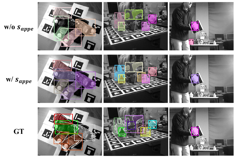
Figure 4: Qualitative results of our Instance Segmentation Model with or without the appearance matching score $s_{appe}$.

A.5.2 Qualitative Comparisons on Geometric Matching Score

We visualize the qualitative comparisons of the geometric matching score $s_{geo}$ in Fig. 5 to show its advantages in scoring the proposals w.r.t. a given object in terms of geometry, e.g., object shapes and sizes.

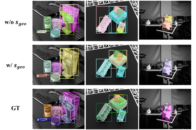
Figure 5: Qualitative results of our Instance Segmentation Model with or without the geometric matching score $s_{geo}$.

A.5.3 More Qualitative Comparisons with Existing Methods

To illustrate the advantages of our Instance Segmentation Model (ISM), we visualize in Fig. 6 the qualitative comparisons with CNOS [38] on all the seven core datasets of the BOP benchmark [50] for instance segmentation of novel objects. For reference, we also provide the ground truth masks, except for the ITODD and HB datasets, as their ground truths are not available.

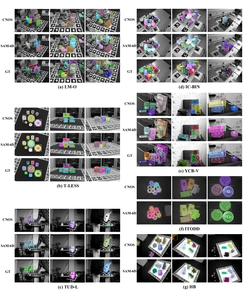
Figure 6: Qualitative results on the seven core datasets of the BOP benchmark [50] for instance segmentation of novel objects.

B Supplementary Material for
Pose Estimation Model

B.1 Network Architectures and Specifics

B.1.1 Feature Extraction

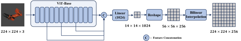
Figure 7: An illustration of the per-pixel feature learning process for an RGB image within the Feature Extraction module of the Pose Estimation Model.

In the Pose Estimation Model (PEM) of our SAM-6D, the Feature Extraction module utilizes the base version of the Visual Transformer (ViT) backbone [8], termed as ViT-Base, to process masked RGB image crops of observed object proposals or rendered object templates, yielding per-pixel feature maps.

Fig. 7 gives an illustration of the per-pixel feature learning process for an RGB image within the Feature Extraction module. More specifically, given an RGB image of the object, the initial step involves image processing, including masking the background, cropping the region of interest, and resizing it to a fixed resolution of $224\times 224$. The object mask and bounding box utilized in the process can be sourced from the Instance Segmentation Model (ISM) for the observed scene image or from the renderer for the object template. The processed image is subsequently fed into ViT-Base to extract per-patch features using 12 attention blocks. The patch features from the third, sixth, ninth, and twelfth blocks are subsequently concatenated and passed through a fully-connected layer. They are then reshaped and bilinearly interpolated to match the input resolution of $224\times 224$ with 256 feature channels. Further specifics about the network can be found in Fig. 7.

For a cropped observed RGB image, the pixel features within the mask are ultimately chosen to correspond to the point set transformed from the masked depth image. For object templates, the pixels within the masks across views are finally aggregated, with the surface point of per pixel known from the renderer. Both point sets of the proposal and the target object are normalized to fit a unit sphere by dividing by the object scale, effectively addressing the variations in object scales.

We use two views of object templates for training, and eight views for evaluation, which is the standard setting for the results reported in this paper.

B.1.2 Coarse Point Matching

In the Coarse Point Matching module, we utilize $T^{c}$ Geometric Transformers [45] to model the relationships between the sparse point set $\mathcal{P}_{m}^{c}\in\mathbb{R}^{N^{c}_{m}\times 3}$ of the observed object proposal $m$ and the set $\mathcal{P}_{o}^{c}\in\mathbb{R}^{N^{c}_{o}\times 3}$ of the target object $\mathcal{O}$. Their respective features $\bm{F}_{m}^{c}$ and $\bm{F}_{o}^{c}$ are thus improved to their enhanced versions $\tilde{\bm{F}}_{m}^{c}$ and $\tilde{\bm{F}}_{o}^{c}$. Each of these enhanced feature maps also includes the background token. An additional fully-connected layer is applied to the features both before and after the transformers. In this paper, we use the upper script ‘c’ to indicate variables associated with the Fine Point Matching module, and the lower scripts ‘m’ and ‘o’ to distinguish between the proposal and the object.

During inference, we compute the soft assignment matrix $\tilde{\mathcal{A}}^{c}\in\mathbb{R}^{(N^{c}_{m}+1)\times(N^{c}_{o}+1)}$, and obtain two binary-value matrices $\bm{M}_{m}^{c}\in\mathcal{R}^{N^{c}_{m}\times 1}$ and $\bm{M}_{o}^{c}\in\mathcal{R}^{N^{c}_{o}\times 1}$, denoting whether the points in $\mathcal{P}_{m}^{c}$ and $\mathcal{P}_{o}^{c}$ correspond to the background, owing to the design of background tokens; ‘0’ indicates correspondence to the background, while ‘1’ indicates otherwise. We then have the probabilities $\bm{P}^{c}\in\mathbb{R}^{N^{c}_{m}\times N^{c}_{o}}$ to indicate the matching degree of the $N^{c}_{m}\times N^{c}_{o}$ point pairs between $\mathcal{P}_{m}^{c}$ and $\mathcal{P}_{o}^{c}$, formulated as follows:

$$\bm{P}^{c}=\bm{M}_{m}^{c}\cdot(\tilde{\mathcal{A}}^{c}[1:,1:])^{\gamma}\cdot\bm{M}_{o}^{cT},$$ (10)

where $\gamma$ is used to sharpen the probabilities and set as $1.5$. The probabilities of points that have no correspondence, whether in $\mathcal{P}_{m}^{c}$ or $\mathcal{P}_{o}^{c}$, are all set to 0. Following this, the probabilities $\bm{P}^{c}$ are normalized to ensure their sum equals 1, and act as weights used to randomly select 6,000 triplets of point pairs from the total pool of $N^{c}_{m}\times N^{c}_{o}$ pairs. Each triplet, which consists of three point pairs, is utilized to calculate a pose using SVD, along with a distance between the point pairs based on the computed pose. Through this procedure, a total of 6,000 pose hypotheses are generated, and to minimize computational cost, only the 300 poses with the smallest point pair distances are selected. Finally, the initial pose for the Fine Point Matching module is determined from these 300 poses, with the pose that has the highest pose matching score being selected.

In the Coarse Point Matching module, we set $T^{c}=3$ and $N^{c}_{m}=N^{c}_{o}=196$, with all the feature channels designated as 256. The configurations of the Geometric Transformers adhere to those used in [45].

B.1.3 Fine Point Matching

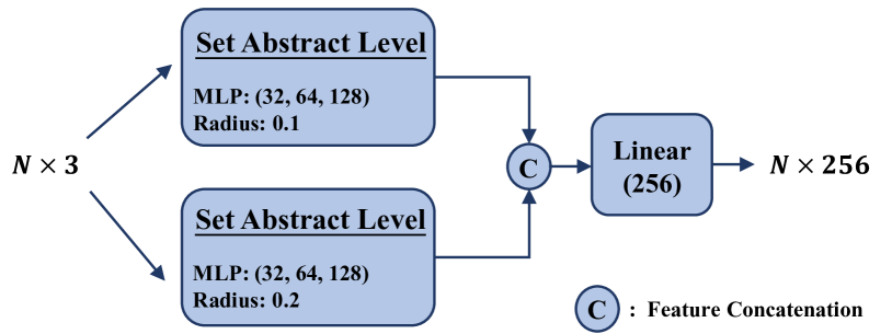
Figure 8: An illustration of the positional encoding for a point set with $N$ points within the Fine Point Matching Module of the Pose Estimation Model.

In the Fine Point Matching module, we utilize $T^{f}$ Sparse-to-Dense Point Transformers to model the relationships between the dense point set $\mathcal{P}_{m}^{f}\in\mathbb{R}^{N^{f}_{m}\times 3}$ of the observed object proposal $m$ and the set $\mathcal{P}_{o}^{f}\in\mathbb{R}^{N^{f}_{o}\times 3}$ of the target object $\mathcal{O}$. Their respective features $\bm{F}_{m}^{f}$ and $\bm{F}_{o}^{f}$ are thus improved to their enhanced versions $\tilde{\bm{F}}_{m}^{f}$ and $\tilde{\bm{F}}_{o}^{f}$. Each of these enhanced feature maps also includes the background token. An additional fully-connected layer is applied to the features both before and after the transformers. We use the upper script ‘$f$’ to indicate variables associated with the Coarse Point Matching module, and the lower scripts ‘m’ and ‘o’ to distinguish between the proposal and the object.

Different from the coarse module, we condition both features $\bm{F}_{m}^{f}$ and $\bm{F}_{o}^{f}$ before applying them to the transformers by adding their respective positional encodings, which are learned via a multi-scale Set Abstract Level [44] from $\mathcal{P}_{m}^{f}$ transformed by the initial pose and $\mathcal{P}_{o}^{f}$ without transformation, respectively. The used architecture for positional encoding learning is illustrated in Fig. 8. For more details, one can refer to [44].

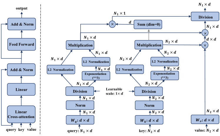
Figure 9: Left: The structure of Linear Cross-attention layer. Right: The structure of Linear Cross-attention.

Another difference from the coarse module is the type of transformers used. To handle dense relationships, we design the Sparse-to-Dense Point Transformers, which utilize Geometric Transformers [45] to process sparse point sets and disseminate information to dense point sets via Linear Cross-attention layers [23, 12]. The configurations of the Geometric Transformers adhere to those used in [45]; the point numbers of the sampled sparse point sets are all set as 196. The Linear Cross-attention layer enables attention along the feature dimension, and details of its architecture can be found in Fig. 9; for more details, one can refer to [23, 12].

During inference, similar to the coarse module, we compute the soft assignment matrix $\tilde{\mathcal{A}}^{f}\in\mathbb{R}^{(N^{f}_{m}+1)\times(N^{f}_{o}+1)}$, and obtain two binary-value matrices $\bm{M}_{m}^{f}\in\mathcal{R}^{N^{f}_{m}\times 1}$ and $\bm{M}_{o}^{f}\in\mathcal{R}^{N^{f}_{o}\times 1}$. We then formulate the probabilities $\bm{P}^{f}\in\mathbb{R}^{N^{f}_{m}\times N^{f}_{o}}$ as follows:

$$\bm{P}^{f}=\bm{M}_{m}^{f}\cdot(\tilde{\mathcal{A}}^{f}[1:,1:])\cdot\bm{M}_{o}^{fT}.$$ (11)

Based on $\bm{P}^{f}$, we search for the best-matched point in $\mathcal{P}_{o}^{f}$ for each point in $\mathcal{P}_{m}^{f}$, assigned with the matching probability. The final object pose is then calculated using a weighted SVD, with the matching probabilities of the point pairs serving as the weights.

Besides, we set $T^{f}=3$ and $N^{f}_{m}=N^{f}_{o}=2,048$, with all the feature channels designated as 256. During training, we follow [26] to obtain the initial object poses by augmenting the ground truth ones with random noises.

Segmentation	BOP Dataset							Mean
Model	LM-O	T-LESS	TUD-L	IC-BIN	ITODD	HB	YCB-V
FastSAM [69]	65.7	47.8	79.7	50.1	56.4	72.4	81.3	64.9
SAM [25]	$\bm{68.7}$	$\bm{49.8}$	$\bm{87.4}$	$\bm{56.1}$	$\bm{57.7}$	$\bm{75.4}$	$\bm{82.8}$	$\bm{68.2}$

Table 10: Pose estimation results with different foundation models for segmentation on the seven core datasets of the BOP benchmark [50]. We report the mean Average Precision (mAP) scores at different Intersection-over-Union (IoU) values ranging from 0.50 to 0.95 with a step size of 0.05.

$\#$ View	BOP Dataset							Mean
	LM-O	T-LESS	TUD-L	IC-BIN	ITODD	HB	YCB-V
1	37.3	30.5	54.0	38.0	48.2	45.7	49.6	43.3
2	67.6	$\bm{50.9}$	86.8	$\bm{57.3}$	57.0	$\bm{75.4}$	82.2	68.1
8	$\bm{68.7}$	49.8	$\bm{87.4}$	56.1	$\bm{57.7}$	$\bm{75.4}$	$\bm{82.8}$	$\bm{68.2}$

Table 11: Pose estimation results with different view numbers of object templates on the seven core datasets of the BOP benchmark [50]. We report the mean Average Precision (mAP) scores at different Intersection-over-Union (IoU) values ranging from 0.50 to 0.95 with a step size of 0.05.

B.2 Training Objectives

We use InfoNCE loss [40] to supervise the learning of attention matrices for both coarse and fine modules. Specifically, given two point sets $\mathcal{P}_{m}\in\mathbb{R}^{N_{m}\times 3}$ and $\mathcal{P}_{o}\in\mathbb{R}^{N_{o}\times 3}$, along with their enhanced features $\tilde{\bm{F}}_{m}$ and $\tilde{\bm{F}}_{o}$, which are learnt via the transformers and equipped with background tokens, we compute the attention matrix $\mathcal{A}=\tilde{\bm{F}}_{m}\times\tilde{\bm{F}}_{o}^{T}\in\mathbb{R}^{(N_{m}+1)\times(N_{o}+1)}$. Then $\mathcal{A}$ can be supervised by the following objective:

$$\mathcal{L}=\texttt{CE}(\mathcal{A}[1:,:],\hat{\mathcal{Y}}_{m})+\texttt{CE}(\mathcal{A}[:,1:]^{T},\hat{\mathcal{Y}}_{o}),$$ (12)

where $\texttt{CE}(\cdot,\cdot)$ denotes the cross-entropy loss function. $\hat{\mathcal{Y}}_{m}\in\mathbb{R}^{N_{m}}$ and $\hat{\mathcal{Y}}_{o}\in\mathbb{R}^{N_{o}}$ denote the ground truths for $\mathcal{P}_{m}$ and $\mathcal{P}_{o}$. Given the ground truth pose $\hat{\bm{R}}$ and $\hat{\bm{t}}$, each element $y_{m}$ in $\hat{\mathcal{Y}}_{m}$, corresponding to the point $\bm{p}_{m}$ in $\mathcal{P}_{m}$, could be obtained as follows:

$$y_{m}=\left\{\begin{matrix}0&\text{if}\enspace d_{k^{*}}\geq\delta_{dis}\\ k^{*}&\text{if}\enspace d_{k^{*}}<\delta_{dis}\end{matrix}\right.,$$ (13)

where

$$k^{*}=\text{Argmin}_{k=1,\dots,N_{m}}||\hat{\bm{R}}(\bm{p}_{m}-\hat{\bm{t}})-\bm{p}_{o,k}||_{2},$$

and

$$d_{k^{*}}=||\hat{\bm{R}}(\bm{p}_{m}-\hat{\bm{t}})-\bm{p}_{o,_{k^{*}}}||_{2}.$$

$k^{*}$ is the index of the closest point $\bm{p}_{o,_{k^{*}}}$ in $\mathcal{P}_{o}$ to $\bm{p}_{m}$, while $d_{k^{*}}$ denotes the distance between $\bm{p}_{m}$ and $\bm{p}_{o,_{k^{*}}}$ in the object coordinate system. $\delta_{dis}$ is a distance threshold determining whether the point $\bm{p}_{m}$ has the correspondence in $\mathcal{P}_{o}$; we set $\delta_{dis}$ as a constant $0.15$, since both $\mathcal{P}_{m}$ and $\mathcal{P}_{o}$ are normalized to a unit sphere. The elements in $\hat{\mathcal{Y}}_{o}$ are also generated in a similar way.

We employ the objective (12) upon all the transformer blocks of both coarse and fine point matching modules, and thus optimize the Pose Estimation Model by solving the following problem:

$$\min\sum_{l=1,\dots,T_{c}}\mathcal{L}_{l}^{c}+\sum_{l=1,\dots,T_{f}}\mathcal{L}_{l}^{f}.$$ (14)

where for the loss $\mathcal{L}$ in Eq. (12), we use the upper scripts ‘$c$’ and ‘$f$’ to distinguish between the losses in the coarse and fine point matching modules, respectively, while the lower script ’$l$’ denotes the sequence of the transformer blocks in each module.

B.3 More Quantitative Results

B.3.1 Quantitative Results with Masks from FastSAM

We provide in Table 10 the pose estimation results of novel objects based on the masks, generated from the FastSAM [69] version of the Instance Segmentation Model, on the seven core datasets of the BOP benchmark. Compared FastSAM [69], SAM [25] generates masks of higher qualities, thereby making the Pose Estimation Model achieve better performance.

B.3.2 Effects of The View Number of Templates

We present a comparison of results using different views of object templates in Table 11. As shown in the table, the overall results from using even 2 templates for each object are comparable to those using 8 templates. However, we find that using 8 views of templates provides better results across more datasets, and thus report results using 8 views by default in the paper due to the robustness. Besides, results with only one template perform poorly as a single view cannot fully depict the entire object.

B.3.3 Comparisons with OVE6D

OVE6D [1] is a classical method for zero-shot pose estimation based on image matching, which first constructs a codebook from the object templates for viewpoint rotation retrieval and subsequently regresses the in-plane rotation. When comparing our SAM-6D with OVE6D using their provided segmentation masks (as shown in Table 12), SAM-6D outperforms OVE6D on LM-O dataset, without the need for using Iterative Closest Point (ICP) algorithm for post-optimization.

Method	LM-O
OVE6D [1]	56.1
OVE6D with ICP [1]	72.8
SAM-6D (Ours)	74.7

Table 12: Quantitative results of OVE6D [1] and our SAM-6D on LM-O dataset. The evaluation metric is the standard ADD(-S) for pose estimation. SAM-6D is evaluated with the same masks provided by [1].

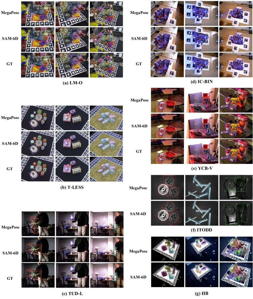
Figure 10: Qualitative results on the seven core datasets of the BOP benchmark [50] for pose estimation of novel objects.

B.4 More Qualitative Comparisons with Existing Methods

To illustrate the advantages of our Pose Estimation Model (ISM), we visualize in Fig. 10 the qualitative comparisons with MegaPose [26] on all the seven core datasets of the BOP benchmark [50] for pose estimation of novel objects. For reference, we also present the corresponding ground truths, barring those for the ITODD and HB datasets, as these are unavailable.

C Conclusion, Limitations, Future Work

In this paper, we take Segment Anything Model (SAM) [25] as an advanced starting point for the focused task of zero-shot 6D object pose estimation, and present a novel framework, termed as SAM-6D, which comprises an Instance Segmentation Model (ISM) and a Pose Estimation Model (PEM) to accomplish the task in two steps. ISM utilizes SAM to segment all potential object proposals and assigns each proposal an object matching score in terms of semantics, appearance, and geometry. PEM then predicts the object pose for each proposal by solving a partial-to-partial point matching problem through two stages of Coarse Point Matching and Fine Point Matching. The effectiveness of SAM-6D is validated on the seven core datasets of the BOP benchmark, where SAM-6D significantly outperforms existing methods.

A significant factor leading to the success of SAM-6D is the employment of foundation models, e.g., SAM [25] and ViT of DINOv2 [41], in ISM. This strategy utilizes the transfer abilities of foundational models to enhance performance, eliminating the need for network re-training or fine-tuning. During training, we exclusively optimize ISM using large-scale synthetic images, which can be easily obtained through rendering. However, just like a coin has two sides, there are also limitations to this approach in addition to its advantages. A primary limitation is that the two models of SAM-6D operate independently, with no interaction. Furthermore, while the foundational models effectively handle common scenarios, they struggle when applied to cluttered industrial scenarios, which are common in the field of pose estimation. Therefore, a potential future direction is to enhance SAM-6D into an end-to-end version that is better adapted for zero-shot pose estimation. We aim to work towards this goal in our future research.

References

- Cai et al. [2022] Dingding Cai, Janne Heikkilä, and Esa Rahtu. Ove6d: Object viewpoint encoding for depth-based 6d object pose estimation. In Proceedings of the IEEE/CVF Conference on Computer Vision and Pattern Recognition, pages 6803–6813, 2022.
- Cen et al. [2023a] Jun Cen, Yizheng Wu, Kewei Wang, Xingyi Li, Jingkang Yang, Yixuan Pei, Lingdong Kong, Ziwei Liu, and Qifeng Chen. Sad: Segment any rgbd. arXiv preprint arXiv:2305.14207, 2023a.
- Cen et al. [2023b] Jiazhong Cen, Zanwei Zhou, Jiemin Fang, Wei Shen, Lingxi Xie, Xiaopeng Zhang, and Qi Tian. Segment anything in 3d with nerfs. arXiv preprint arXiv:2304.12308, 2023b.
- Chang et al. [2015] Angel X Chang, Thomas Funkhouser, Leonidas Guibas, Pat Hanrahan, Qixing Huang, Zimo Li, Silvio Savarese, Manolis Savva, Shuran Song, Hao Su, et al. Shapenet: An information-rich 3d model repository. arXiv preprint arXiv:1512.03012, 2015.
- Chen et al. [2023a] Jianqiu Chen, Mingshan Sun, Tianpeng Bao, Rui Zhao, Liwei Wu, and Zhenyu He. 3d model-based zero-shot pose estimation pipeline. arXiv preprint arXiv:2305.17934, 2023a.
- Chen et al. [2023b] Jiaqi Chen, Zeyu Yang, and Li Zhang. Semantic segment anything. https://github.com/fudan-zvg/Semantic-Segment-Anything, 2023b.
- Chen and Dou [2021] Kai Chen and Qi Dou. Sgpa: Structure-guided prior adaptation for category-level 6d object pose estimation. In Proceedings of the IEEE/CVF International Conference on Computer Vision, pages 2773–2782, 2021.
- Dosovitskiy et al. [2020] Alexey Dosovitskiy, Lucas Beyer, Alexander Kolesnikov, Dirk Weissenborn, Xiaohua Zhai, Thomas Unterthiner, Mostafa Dehghani, Matthias Minderer, Georg Heigold, Sylvain Gelly, et al. An image is worth 16x16 words: Transformers for image recognition at scale. arXiv preprint arXiv:2010.11929, 2020.
- Downs et al. [2022] Laura Downs, Anthony Francis, Nate Koenig, Brandon Kinman, Ryan Hickman, Krista Reymann, Thomas B McHugh, and Vincent Vanhoucke. Google scanned objects: A high-quality dataset of 3d scanned household items. In 2022 International Conference on Robotics and Automation (ICRA), pages 2553–2560. IEEE, 2022.
- Fan et al. [2023] Zhiwen Fan, Panwang Pan, Peihao Wang, Yifan Jiang, Dejia Xu, Hanwen Jiang, and Zhangyang Wang. Pope: 6-dof promptable pose estimation of any object, in any scene, with one reference. arXiv preprint arXiv:2305.15727, 2023.
- Goodwin et al. [2022] Walter Goodwin, Sagar Vaze, Ioannis Havoutis, and Ingmar Posner. Zero-shot category-level object pose estimation. In European Conference on Computer Vision, pages 516–532. Springer, 2022.
- Han et al. [2023a] Dongchen Han, Xuran Pan, Yizeng Han, Shiji Song, and Gao Huang. Flatten transformer: Vision transformer using focused linear attention. In Proceedings of the IEEE/CVF International Conference on Computer Vision, pages 5961–5971, 2023a.
- Han et al. [2023b] Dongsheng Han, Chaoning Zhang, Yu Qiao, Maryam Qamar, Yuna Jung, SeungKyu Lee, Sung-Ho Bae, and Choong Seon Hong. Segment anything model (sam) meets glass: Mirror and transparent objects cannot be easily detected. arXiv preprint arXiv:2305.00278, 2023b.
- Haugaard and Buch [2022] Rasmus Laurvig Haugaard and Anders Glent Buch. Surfemb: Dense and continuous correspondence distributions for object pose estimation with learnt surface embeddings. In Proceedings of the IEEE/CVF Conference on Computer Vision and Pattern Recognition, pages 6749–6758, 2022.
- He et al. [2023] Haibin He, Jing Zhang, Mengyang Xu, Juhua Liu, Bo Du, and Dacheng Tao. Scalable mask annotation for video text spotting. arXiv preprint arXiv:2305.01443, 2023.
- He et al. [2017] Kaiming He, Georgia Gkioxari, Piotr Dollár, and Ross Girshick. Mask r-cnn. In Proceedings of the IEEE international conference on computer vision, pages 2961–2969, 2017.
- He et al. [2022a] Xingyi He, Jiaming Sun, Yuang Wang, Di Huang, Hujun Bao, and Xiaowei Zhou. Onepose++: Keypoint-free one-shot object pose estimation without cad models. Advances in Neural Information Processing Systems, 35:35103–35115, 2022a.
- He et al. [2020] Yisheng He, Wei Sun, Haibin Huang, Jianran Liu, Haoqiang Fan, and Jian Sun. Pvn3d: A deep point-wise 3d keypoints voting network for 6dof pose estimation. In Proceedings of the IEEE/CVF conference on computer vision and pattern recognition, pages 11632–11641, 2020.
- He et al. [2021] Yisheng He, Haibin Huang, Haoqiang Fan, Qifeng Chen, and Jian Sun. Ffb6d: A full flow bidirectional fusion network for 6d pose estimation. In Proceedings of the IEEE/CVF Conference on Computer Vision and Pattern Recognition, pages 3003–3013, 2021.
- He et al. [2022b] Yisheng He, Yao Wang, Haoqiang Fan, Jian Sun, and Qifeng Chen. Fs6d: Few-shot 6d pose estimation of novel objects. In Proceedings of the IEEE/CVF Conference on Computer Vision and Pattern Recognition, pages 6814–6824, 2022b.
- Ji et al. [2023a] Ge-Peng Ji, Deng-Ping Fan, Peng Xu, Ming-Ming Cheng, Bowen Zhou, and Luc Van Gool. Sam struggles in concealed scenes–empirical study on” segment anything”. arXiv preprint arXiv:2304.06022, 2023a.
- Ji et al. [2023b] Wei Ji, Jingjing Li, Qi Bi, Wenbo Li, and Li Cheng. Segment anything is not always perfect: An investigation of sam on different real-world applications. arXiv preprint arXiv:2304.05750, 2023b.
- Katharopoulos et al. [2020] Angelos Katharopoulos, Apoorv Vyas, Nikolaos Pappas, and François Fleuret. Transformers are rnns: Fast autoregressive transformers with linear attention. In International conference on machine learning, pages 5156–5165. PMLR, 2020.
- Ke and Roumeliotis [2017] Tong Ke and Stergios I Roumeliotis. An efficient algebraic solution to the perspective-three-point problem. In Proceedings of the IEEE Conference on Computer Vision and Pattern Recognition, pages 7225–7233, 2017.
- Kirillov et al. [2023] Alexander Kirillov, Eric Mintun, Nikhila Ravi, Hanzi Mao, Chloe Rolland, Laura Gustafson, Tete Xiao, Spencer Whitehead, Alexander C Berg, Wan-Yen Lo, et al. Segment anything. arXiv preprint arXiv:2304.02643, 2023.
- Labbé et al. [2022] Yann Labbé, Lucas Manuelli, Arsalan Mousavian, Stephen Tyree, Stan Birchfield, Jonathan Tremblay, Justin Carpentier, Mathieu Aubry, Dieter Fox, and Josef Sivic. Megapose: 6d pose estimation of novel objects via render & compare. In Proceedings of the 6th Conference on Robot Learning (CoRL), 2022.
- Lin et al. [2021a] Jiehong Lin, Hongyang Li, Ke Chen, Jiangbo Lu, and Kui Jia. Sparse steerable convolutions: An efficient learning of se (3)-equivariant features for estimation and tracking of object poses in 3d space. Advances in Neural Information Processing Systems, 34:16779–16790, 2021a.
- Lin et al. [2021b] Jiehong Lin, Zewei Wei, Zhihao Li, Songcen Xu, Kui Jia, and Yuanqing Li. Dualposenet: Category-level 6d object pose and size estimation using dual pose network with refined learning of pose consistency. In Proceedings of the IEEE/CVF International Conference on Computer Vision, pages 3560–3569, 2021b.
- Lin et al. [2022] Jiehong Lin, Zewei Wei, Changxing Ding, and Kui Jia. Category-level 6d object pose and size estimation using self-supervised deep prior deformation networks. In European Conference on Computer Vision, pages 19–34. Springer, 2022.
- Lin et al. [2023] Jiehong Lin, Zewei Wei, Yabin Zhang, and Kui Jia. Vi-net: Boosting category-level 6d object pose estimation via learning decoupled rotations on the spherical representations. In Proceedings of the IEEE/CVF International Conference on Computer Vision, pages 14001–14011, 2023.
- Liu et al. [2022] Yuan Liu, Yilin Wen, Sida Peng, Cheng Lin, Xiaoxiao Long, Taku Komura, and Wenping Wang. Gen6d: Generalizable model-free 6-dof object pose estimation from rgb images. In European Conference on Computer Vision, pages 298–315. Springer, 2022.
- Liu et al. [2023a] Yang Liu, Muzhi Zhu, Hengtao Li, Hao Chen, Xinlong Wang, and Chunhua Shen. Matcher: Segment anything with one shot using all-purpose feature matching. arXiv preprint arXiv:2305.13310, 2023a.
- Liu et al. [2023b] Zhaoyang Liu, Yinan He, Wenhai Wang, Weiyun Wang, Yi Wang, Shoufa Chen, Qinglong Zhang, Yang Yang, Qingyun Li, Jiashuo Yu, et al. Internchat: Solving vision-centric tasks by interacting with chatbots beyond language. arXiv preprint arXiv:2305.05662, 2023b.
- Ma and Wang [2023] Jun Ma and Bo Wang. Segment anything in medical images. arXiv preprint arXiv:2304.12306, 2023.
- Mazurowski et al. [2023] Maciej A Mazurowski, Haoyu Dong, Hanxue Gu, Jichen Yang, Nicholas Konz, and Yixin Zhang. Segment anything model for medical image analysis: an experimental study. Medical Image Analysis, 89:102918, 2023.
- Nguyen et al. [2022] Van Nguyen Nguyen, Yinlin Hu, Yang Xiao, Mathieu Salzmann, and Vincent Lepetit. Templates for 3d object pose estimation revisited: Generalization to new objects and robustness to occlusions. In Proceedings of the IEEE/CVF conference on computer vision and pattern recognition, pages 6771–6780, 2022.
- Nguyen et al. [2023a] Van Nguyen Nguyen, Thibault Groueix, Yinlin Hu, Mathieu Salzmann, and Vincent Lepetit. Nope: Novel object pose estimation from a single image. arXiv preprint arXiv:2303.13612, 2023a.
- Nguyen et al. [2023b] Van Nguyen Nguyen, Thibault Groueix, Georgy Ponimatkin, Vincent Lepetit, and Tomas Hodan. Cnos: A strong baseline for cad-based novel object segmentation. arXiv preprint arXiv:2307.11067, 2023b.
- Okorn et al. [2021] Brian Okorn, Qiao Gu, Martial Hebert, and David Held. Zephyr: Zero-shot pose hypothesis rating. In 2021 IEEE International Conference on Robotics and Automation (ICRA), pages 14141–14148. IEEE, 2021.
- Oord et al. [2018] Aaron van den Oord, Yazhe Li, and Oriol Vinyals. Representation learning with contrastive predictive coding. arXiv preprint arXiv:1807.03748, 2018.
- Oquab et al. [2023a] Maxime Oquab, Timothée Darcet, Théo Moutakanni, Huy Vo, Marc Szafraniec, Vasil Khalidov, Pierre Fernandez, Daniel Haziza, Francisco Massa, Alaaeldin El-Nouby, et al. Dinov2: Learning robust visual features without supervision. arXiv preprint arXiv:2304.07193, 2023a.
- Oquab et al. [2023b] Maxime Oquab, Timothée Darcet, Théo Moutakanni, Huy Vo, Marc Szafraniec, Vasil Khalidov, Pierre Fernandez, Daniel Haziza, Francisco Massa, Alaaeldin El-Nouby, et al. Dinov2: Learning robust visual features without supervision. arXiv preprint arXiv:2304.07193, 2023b.
- Pan et al. [2023] Panwang Pan, Zhiwen Fan, Brandon Y Feng, Peihao Wang, Chenxin Li, and Zhangyang Wang. Learning to estimate 6dof pose from limited data: A few-shot, generalizable approach using rgb images. arXiv preprint arXiv:2306.07598, 2023.
- Qi et al. [2017] Charles Ruizhongtai Qi, Li Yi, Hao Su, and Leonidas J Guibas. Pointnet++: Deep hierarchical feature learning on point sets in a metric space. Advances in neural information processing systems, 30, 2017.
- Qin et al. [2022] Zheng Qin, Hao Yu, Changjian Wang, Yulan Guo, Yuxing Peng, and Kai Xu. Geometric transformer for fast and robust point cloud registration. In Proceedings of the IEEE/CVF conference on computer vision and pattern recognition, pages 11143–11152, 2022.
- Shen et al. [2023] Qiuhong Shen, Xingyi Yang, and Xinchao Wang. Anything-3d: Towards single-view anything reconstruction in the wild. arXiv preprint arXiv:2304.10261, 2023.
- Shugurov et al. [2022] Ivan Shugurov, Fu Li, Benjamin Busam, and Slobodan Ilic. Osop: A multi-stage one shot object pose estimation framework. In Proceedings of the IEEE/CVF Conference on Computer Vision and Pattern Recognition, pages 6835–6844, 2022.
- Su et al. [2022] Yongzhi Su, Mahdi Saleh, Torben Fetzer, Jason Rambach, Nassir Navab, Benjamin Busam, Didier Stricker, and Federico Tombari. Zebrapose: Coarse to fine surface encoding for 6dof object pose estimation. In Proceedings of the IEEE/CVF Conference on Computer Vision and Pattern Recognition, pages 6738–6748, 2022.
- Sun et al. [2022] Jiaming Sun, Zihao Wang, Siyu Zhang, Xingyi He, Hongcheng Zhao, Guofeng Zhang, and Xiaowei Zhou. Onepose: One-shot object pose estimation without cad models. In Proceedings of the IEEE/CVF Conference on Computer Vision and Pattern Recognition, pages 6825–6834, 2022.
- Sundermeyer et al. [2023] Martin Sundermeyer, Tomáš Hodaň, Yann Labbe, Gu Wang, Eric Brachmann, Bertram Drost, Carsten Rother, and Jiří Matas. Bop challenge 2022 on detection, segmentation and pose estimation of specific rigid objects. In Proceedings of the IEEE/CVF Conference on Computer Vision and Pattern Recognition, pages 2784–2793, 2023.
- Tang et al. [2023] Lv Tang, Haoke Xiao, and Bo Li. Can sam segment anything? when sam meets camouflaged object detection. arXiv preprint arXiv:2304.04709, 2023.
- Tian et al. [2020] Meng Tian, Marcelo H Ang, and Gim Hee Lee. Shape prior deformation for categorical 6d object pose and size estimation. In Computer Vision–ECCV 2020: 16th European Conference, Glasgow, UK, August 23–28, 2020, Proceedings, Part XXI 16, pages 530–546. Springer, 2020.
- Vaswani et al. [2017] Ashish Vaswani, Noam Shazeer, Niki Parmar, Jakob Uszkoreit, Llion Jones, Aidan N Gomez, Łukasz Kaiser, and Illia Polosukhin. Attention is all you need. Advances in neural information processing systems, 30, 2017.
- Wang et al. [2019a] Chen Wang, Danfei Xu, Yuke Zhu, Roberto Martín-Martín, Cewu Lu, Li Fei-Fei, and Silvio Savarese. Densefusion: 6d object pose estimation by iterative dense fusion. In Proceedings of the IEEE/CVF conference on computer vision and pattern recognition, pages 3343–3352, 2019a.
- Wang et al. [2023a] Dongqing Wang, Tong Zhang, Alaa Abboud, and Sabine Süsstrunk. Inpaintnerf360: Text-guided 3d inpainting on unbounded neural radiance fields. arXiv preprint arXiv:2305.15094, 2023a.
- Wang et al. [2021] Gu Wang, Fabian Manhardt, Federico Tombari, and Xiangyang Ji. Gdr-net: Geometry-guided direct regression network for monocular 6d object pose estimation. In Proceedings of the IEEE/CVF Conference on Computer Vision and Pattern Recognition, pages 16611–16621, 2021.
- Wang et al. [2019b] He Wang, Srinath Sridhar, Jingwei Huang, Julien Valentin, Shuran Song, and Leonidas J Guibas. Normalized object coordinate space for category-level 6d object pose and size estimation. In Proceedings of the IEEE/CVF Conference on Computer Vision and Pattern Recognition, pages 2642–2651, 2019b.
- Wang et al. [2023b] Qian Wang, Biao Zhang, Michael Birsak, and Peter Wonka. Instructedit: Improving automatic masks for diffusion-based image editing with user instructions. arXiv preprint arXiv:2305.18047, 2023b.
- Xiang et al. [2017] Yu Xiang, Tanner Schmidt, Venkatraman Narayanan, and Dieter Fox. Posecnn: A convolutional neural network for 6d object pose estimation in cluttered scenes. arXiv preprint arXiv:1711.00199, 2017.
- Xie et al. [2023] Defeng Xie, Ruichen Wang, Jian Ma, Chen Chen, Haonan Lu, Dong Yang, Fobo Shi, and Xiaodong Lin. Edit everything: A text-guided generative system for images editing. arXiv preprint arXiv:2304.14006, 2023.
- Yang et al. [2023a] Jinyu Yang, Mingqi Gao, Zhe Li, Shang Gao, Fangjing Wang, and Feng Zheng. Track anything: Segment anything meets videos. arXiv preprint arXiv:2304.11968, 2023a.
- Yang et al. [2023b] Yunhan Yang, Xiaoyang Wu, Tong He, Hengshuang Zhao, and Xihui Liu. Sam3d: Segment anything in 3d scenes. arXiv preprint arXiv:2306.03908, 2023b.
- Yu et al. [2023] Tao Yu, Runseng Feng, Ruoyu Feng, Jinming Liu, Xin Jin, Wenjun Zeng, and Zhibo Chen. Inpaint anything: Segment anything meets image inpainting. arXiv preprint arXiv:2304.06790, 2023.
- Zhang et al. [2023a] Chaoning Zhang, Dongshen Han, Yu Qiao, Jung Uk Kim, Sung-Ho Bae, Seungkyu Lee, and Choong Seon Hong. Faster segment anything: Towards lightweight sam for mobile applications. arXiv preprint arXiv:2306.14289, 2023a.
- Zhang et al. [2023b] Chaoning Zhang, Sheng Zheng, Chenghao Li, Yu Qiao, Taegoo Kang, Xinru Shan, Chenshuang Zhang, Caiyan Qin, Francois Rameau, Sung-Ho Bae, et al. A survey on segment anything model (sam): Vision foundation model meets prompt engineering. arXiv preprint arXiv:2306.06211, 2023b.
- Zhang et al. [2023c] Dingyuan Zhang, Dingkang Liang, Hongcheng Yang, Zhikang Zou, Xiaoqing Ye, Zhe Liu, and Xiang Bai. Sam3d: Zero-shot 3d object detection via segment anything model. arXiv preprint arXiv:2306.02245, 2023c.
- Zhang et al. [2023d] Renrui Zhang, Zhengkai Jiang, Ziyu Guo, Shilin Yan, Junting Pan, Hao Dong, Peng Gao, and Hongsheng Li. Personalize segment anything model with one shot. arXiv preprint arXiv:2305.03048, 2023d.
- Zhang et al. [2023e] Zhenghao Zhang, Zhichao Wei, Shengfan Zhang, Zuozhuo Dai, and Siyu Zhu. Uvosam: A mask-free paradigm for unsupervised video object segmentation via segment anything model. arXiv preprint arXiv:2305.12659, 2023e.
- Zhao et al. [2023] Xu Zhao, Wenchao Ding, Yongqi An, Yinglong Du, Tao Yu, Min Li, Ming Tang, and Jinqiao Wang. Fast segment anything. arXiv preprint arXiv:2306.12156, 2023.