Quantum state engineering in a five-state chainwise system by coincident pulse technique

Abstract

We generalize the coincident pulse technique in three-state stimulated Raman adiabatic passage (STIRAP) system [A. A. Rangelov and N. V. Vitanov, Phys. Rev. A 85, 043407 (2012)] to a five-state chainwise STIRAP system. In our method, we first reduce the M-type structure into a generalized $\Lambda$-type one with the simplest resonant coupling, which principally allows us to employ the standard coincident pulse technique from three-state system into the five-state chainwise system. The simplification is realized under the assumption of adiabatic elimination (AE) together with a requirement of the relation among the four incident pulses. The results show that, by using $N(N\gg 1)$ pairs of coincident incident pulses, this technique enables complete population transfer, as well as the creation of arbitrary desired coherent superposition between initial and final states, while there are negligible population in all the intermediate states. The results are of potential interest in applications where high-fidelity multi-state quantum control is essential, e.g., quantum information, atom optics, formation of ultracold molecules, cavity QED, nuclear coherent population transfer, light transfer in waveguide arrays, etc.

I Introduction

The quest for techniques with which to control the transfer of population between specified states is a major topic in the field of atomic, molecular and optical physics. The well-known stimulated Raman adiabatic passage (STIRAP) technique has become an important tool; see reviews Bergmann et al. (1998); Vitanov et al. (2001a); Král et al. (2007); Bergmann et al. (2015); Vitanov et al. (2017); Bergmann et al. (2019). The standard STIRAP process utilizes a Raman transition with two counter-intuitively ordered laser pulses, allowing for the efficient and robust transfer of the population between an initial and a final state of a three-state. The successes of STIRAP relies on the existence of the dark state, which should be followed adiabatically Vitanov (2020). The middle state, which is subjected to population decay in many physical implementations Vitanov and Stenholm (1997); Wellnitz et al. (2020); Ciamei et al. (2017); Li et al. (2017); Zhang and Dou (2021); Stefanatos and Paspalakis (2021); Zhang et al. (2023a), is not populated during the process because it is not present in the dark state.

The success of STRAP has prompted its extension to chainwise-connected multi-state systems Sola et al. (2018); Vitanov et al. (2001b); Vitanov (1998a); Oreg et al. (1992); Pillet et al. (1993); Malinovsky and Tannor (1997); Solá et al. (1999); Linington et al. (2008); Grigoryan et al. (2015); Kamsap et al. (2013); Mukherjee et al. (2017); Sola et al. (2022), in which each state is connected only to its two neighbors: $|1\rangle\leftrightarrow|2\rangle\leftrightarrow|3\rangle\leftrightarrow\cdot\cdot\cdot\leftrightarrow|n\rangle$. In general, the goal is to transfer the population between the two ends without filling the intermediate states. The potential applications involve many branches of fundamental physics and chemistry. Just a few examples: (i) atomic mirrors and beams splitters in atom optics Theuer and Bergmann (1998); Goldner et al. (1994); (ii) cavity QED Parkins et al. (1993, 1995); (iii) spin-wave transfer via adiabatic passage in a five-level system Simon et al. (2007); (iv) creation and detection of ultracold molecules Danzl et al. (2010); Mark et al. (2009); Kuznetsova et al. (2008); Mackie and Phou (2010); Qian et al. (2010); Price and Yelin (2019), chainwise-STIRAP in M-type molecular system has been demonstrated a good alternative in creating ultracold deeply-bound molecules when the typical STIRAP in $\Lambda$-type system does not work due to weak Frank-Condon factors between the molecular states that are involved Danzl et al. (2010); Kuznetsova et al. (2008), the prepared molecule can be used in the study of ultracold chemistry Hutson (2010), precision measurements Ulmanis et al. (2012), quantum computations and quantum simulations Carr et al. (2009); (v) multi-state nuclear coherent population transfer Amiri and Saadati-Niari (2023), which can be used in the study of the nucleus, the construction of nuclear batteries Liao et al. (2011, 2013); Kirschbaum et al. (2022), as well as the construction of nuclear clocks that are much more accurate than atomic clocks Seiferle et al. (2019); (vi) adiabatic light transfer in waveguide arrays Della Valle et al. (2008); Tseng and Wu (2010); Ciret et al. (2013), which has profound impacts on exploring quantum technologies for promoting advanced optical devices, and provides a direct visualization in space of typical phenomena in time. Quite often, it is necessary to achieve state preparation or transfer with high fidelity. This requires large temporal areas of the driving pulsed fields in order to suppress the non-adiabatic couplings, which is very hard to reach experimentally. Although strategies for optimization of multi-state chainwise system with minimal pulse areas have been developed Price and Yelin (2019); Vitanov (2020); N. Irani and Saadati-Niari (2022); Zhang et al. (2023b), these come at the expense of strict relations on the pulse shapes Vitanov (2020); N. Irani and Saadati-Niari (2022), require specific time-dependent nonzero detunings Price and Yelin (2019), or require additional couplings between the states that are involved Vitanov (2020).

Recently, Rangelov and Vitanov have proposed a technique to complete population transfer in three-state systems by a train of $N$ pairs of coincident pulses Rangelov and Vitanov (2012), in which the population in the intermediate excited state is suppressed to negligible small value by increasing the pulse pairs. In this technique the number of pulse pairs is arbitrary and the robustness of system against deviation from exact pulse areas and spontaneous emission from excited state rise with increasing numbers of pulse pairs Nedaee-Shakarab et al. (2016). Since the technique uses fields on exact resonance, the pulse shape is not important. The technique has recently been generalized to tripod system Nedaee-Shakarab et al. (2017). However, the application of coincident pulse technique in multi-state chainwise-connected systems has not been reported to date.

In the present paper, we generalize the coincident pulse technique in three-state system to a five-state chainwise system. We first reduce the dynamics of the five-state chainwise system to that of effective three-state counterpart. By further setting a requirement towards the relation among the four incident pulses, i.e., the pulses at both ends are the root mean square (rms) of the middle two pulses, it is found that this system can be further generalized into a $\Lambda$-type structure with the simplest resonant coupling. Thereafter, this generalized model permits us to borrow the standard coincident pulse technique from three-state system into the five-state chainwise system. The results show that, by using $N(N\gg 1)$ pairs of coincident incident pulses, our technique enables complete population transfer, as well as the creation of arbitrary coherent superposition between initial and final states with negligibly small transient populations in all the intermediate states. All these properties make this technique an interesting alternative of the existing techniques for coherent control of five-state chainwise system.

II Model and Methods

The idea of this work can be described using a simple five-level system with states chainwise coupled by optical fields as illustrated in Fig. 1. The states $|g_{1}\rangle$, $|g_{2}\rangle$ and $|g_{3}\rangle$ are three ground states of long lifetimes while the intermediate states $|e_{1}\rangle$, and $|e_{2}\rangle$ refer to two excited states of short lifetimes. The coupling between states is presented by the time-dependent Rabi frequency $\Omega_{i}(i=1,2,3,4)$ in this figure.

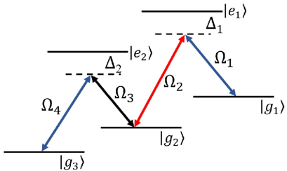
Figure 1: Linkage pattern of the chainwise-like five-state system. Note that in our method the relation among the four incident pulses satisfies $\Omega_{1}(t)=\Omega_{4}(t)=\sqrt{\Omega_{2}^{2}(t)+\Omega_{3}^{2}(t)}$.

The total wave function can be expanded as

$$|\psi(t)\rangle=c_{1}(t)|g_{1}\rangle +c_{2}(t)|e_{1}\rangle+c_{3}(t)|g_{2}\rangle$$ (1)

$$+c_{4}(t)|e_{2}\rangle+c_{5}(t)|g_{3}\rangle.$$

the vector $c_{i}(t)(i=1,2,3,4,5)$ are the probability amplitudes of the corresponding state. The evolution is then governed by the time-dependent Schrödinger equation:

$$i\hbar\displaystyle\frac{\partial}{\partial t}c(t)=H(t)c(t).$$ (2)

Here, $c(t)$ is a five-component column matrix with the elements $\{c_{1}(t),c_{2}(t),c_{3}(t),c_{4}(t),c_{5}(t)\}$, and $P_{i}=|c_{i}(t)|^{2}$ are the corresponding probability. In the interaction representation and after adopting the rotating-wave approximation, this system can be quantitatively described in terms of a five-state Hamiltonian $(\hbar=1)$

$$H(t)=\frac{1}{2}\left(\begin{array}[]{ccccc}0&\Omega_{1}(t)&0&0&0\\ \Omega_{1}(t)&2\Delta_{1}&\Omega_{2}(t)&0&0\\ 0&\Omega_{2}(t)&0&\Omega_{3}(t)&0\\ 0&0&\Omega_{3}(t)&2\Delta_{2}&\Omega_{4}(t)\\ 0&0&0&\Omega_{4}(t)&0\\ \end{array}\right),$$ (8)

where the quantities $\Delta_{1}$ and $\Delta_{2}$ stand for single-photon detunings of the corresponding transitions.

If we assume that pairs of fields coupling two neighboring ground state vibrational levels are in a two-photon (Raman) resonance, the system has a dark state given by

$$|\psi_{0}\rangle=\frac{\Omega_{2}(t)\Omega_{4}(t)|g_{1}\rangle-\Omega_{1}(t)\Omega_{4}(t)|g_{2}\rangle+\Omega_{1}(t)\Omega_{3}(t)|g_{3}\rangle}{\mathcal{N}(t)},$$ (9)

where $\mathcal{N}(t)$ is a normalization factor. In “classical” STIRAP, where the incident fields are applied in a counterintuitive time sequence. Adiabatically changing the Rabi frequencies of the optical fields so that the system stays in the dark state during evolution, one can transfer the system from the initial $|g_{1}\rangle$ to the ground vibrational $|g_{3}\rangle$ state with unit efficiency. The dark state does not have contributions from the $|e_{1}\rangle$ and $|e_{1}\rangle$ excited states, and thus the decay from these states does not affect the transfer efficiency. However, the intermediate ground state $|g_{2}\rangle$ will receive some transient population. In some particular example Simon et al. (2007); Kuznetsova et al. (2008); Mackie and Phou (2010); Wang et al. (2012); Zhang et al. (2015), $|g_{2}\rangle$ is a radiative state, decay from this state will degrade the coherent superposition (9) and result in population loss from the dark state and reduction of the transfer efficiency.

When the single-photon detunings are very large, meaning

$$|\Delta_{1}| \gg\sqrt{\Omega^{2}_{1}(t)+\Omega^{2}_{2}(t)},$$ (10a)

$$|\Delta_{2}| \gg\sqrt{\Omega^{2}_{3}(t)+\Omega^{2}_{4}(t)},$$ (10b)

as we shall assume for our case, then states $|e_{1,2}\rangle$ are scarcely populated, and which can be adiabatically eliminated to obtain the following effective three-state Hamiltonian in the subspace {$|g_{1}\rangle$, $|g_{2}\rangle$, $|g_{3}\rangle$}:

$$H_{e}(t)=\frac{1}{2}\left(\begin{array}[]{ccc}\Delta_{e1}&\Omega_{e1}&0\\ \Omega_{e1}&\Delta_{e2}&\Omega_{e2}\\ 0&\Omega_{e2}&\Delta_{e3}\\ \end{array}\right),$$ (14)

where the effective couplings are defined as (for simplicity, we have assumed that $\Delta_{1}=\Delta_{2}=\Delta$)

$$\Omega_{e_{1}}(t) =-\frac{\Omega_{1}(t)\Omega_{2}(t)}{2\Delta},$$ (15a)

$$\Omega_{e_{2}}(t) =-\frac{\Omega_{3}(t)\Omega_{4}(t)}{2\Delta},$$ (15b)

respectively, and three diagonal elements are

$$\Delta_{e_{1}} =-\frac{\Omega_{1}^{2}(t)}{2\Delta},$$ (16a)

$$\Delta_{e_{2}} =-\frac{\Omega_{2}^{2}(t)+\Omega_{3}^{2}(t)}{2\Delta},$$ (16b)

$$\Delta_{e_{3}} =-\frac{\Omega_{4}^{2}(t)}{2\Delta}.$$ (16c)

Thereafter, two-photon transitions $|g_{1}\rangle\leftrightarrow|g_{2}\rangle$ and $|g_{1}\rangle\leftrightarrow|g_{3}\rangle$ will dominate.

Obviously, the system after AE subjects to dynamic Stark shifts from the trapping light, which can be expected to reduce the transfer efficiency. If we assume that the three diagonal elements are equal to each other, i.e., $\Delta_{e_{1}}=\Delta_{e_{2}}=\Delta_{e_{3}}=\Delta_{e}$. This requires that the four Rabi frequencies $\Omega_{j}(j=1,2,3,4)$ should satisfy

$$\Omega_{1}(t)=\Omega_{4}(t)=\sqrt{\Omega_{2}^{2}(t)+\Omega_{3}^{2}(t)}.$$ (17)

By further setting $c_{j}=c^{{}^{\prime}}_{j}e^{-i\Delta_{e}t}(i=1,3,5)$, the above equation can be written in the following form:

$$i\displaystyle\frac{\partial}{\partial t}\left(\begin{array}[]{ccc}c^{{}^{\prime}}_{1}\\ c^{{}^{\prime}}_{3}\\ c^{{}^{\prime}}_{5}\\ \end{array}\right)=\frac{1}{2}\left(\begin{array}[]{ccc}0&\Omega_{e_{1}}(t)&0\\ \Omega_{e_{1}}(t)&0&\Omega_{e_{2}}(t)\\ 0&\Omega_{e_{2}}(t)&0\\ \end{array}\right)\left(\begin{array}[]{ccc}c^{{}^{\prime}}_{1}\\ c^{{}^{\prime}}_{3}\\ c^{{}^{\prime}}_{5}\\ \end{array}\right).$$ (27)

Therefore, the basic model (8) is generalized into a $\Lambda$-type structure with the simplest resonant coupling:

$$H_{e}=\frac{1}{2}\left(\begin{array}[]{ccc}0&\Omega_{e_{1}}(t)&0\\ \Omega_{e_{1}}(t)&0&\Omega_{e_{2}}(t)\\ 0&\Omega_{e_{2}}(t)&0\\ \end{array}\right),$$ (31)

in which

$$\Omega_{e_{1}}(t) =-\frac{\Omega_{2}(t)\sqrt{\Omega_{2}^{2}(t)+\Omega_{3}^{2}(t)}}{2\Delta},$$ (32a)

$$\Omega_{e_{2}}(t) =-\frac{\Omega_{3}(t)\sqrt{\Omega_{2}^{2}(t)+\Omega_{3}^{2}(t)}}{2\Delta}.$$ (32b)

In order to implement the coincident pulse technique in this generalized model, we impose the condition that the effective Rabi frequencies $\Omega_{e_{1}}(t)$ and $\Omega_{e_{2}}(t)$ are pulse-shaped functions that share the same time dependence, but possibly with different magnitudes. This essentially means that the Rabi frequencies $\Omega_{2}(t)$ and $\Omega_{3}(t)$ are pulse-shaped functions with the same time dependences, but possibly with different magnitudes, i.e.,

$$\Omega_{2}(t) =\eta_{2}f(t),$$ (33a)

$$\Omega_{3}(t) =\eta_{3}f(t).$$ (33b)

In this case, the Schrödinger equation (31) is solved exactly by making a transformation to the so-called bright-dark basis Huang et al. (2014); Alrifai et al. (2021). The exact propagator is given by Vitanov (1998b)

$$U(\varphi)=\left(\begin{array}[]{ccc}1-2\sin^{2}\varphi\sin^{2}\frac{A}{4}&-i\sin\varphi\sin\frac{A}{2}&-2\sin 2\varphi\sin^{2}\frac{A}{4}\\ -i\sin\varphi\sin\frac{A}{2}&\cos\frac{A}{2}&-i\cos\varphi\sin\frac{A}{2}\\ -2\sin 2\varphi\sin^{2}\frac{A}{4}&-i\cos\varphi\sin\frac{A}{2}&1-2\cos^{2}\varphi\sin^{2}\frac{A}{4}\\ \end{array}\right),$$ (37)

where $\tan\varphi=\frac{\Omega_{e_{1}}}{\Omega_{e_{2}}}=\frac{\Omega_{2}}{\Omega_{3}}=\frac{\eta_{2}}{\eta_{3}}$, the rms pulse area $A$ is defined as $A=\int^{t}_{t_{i}}\sqrt{\Omega^{2}_{e_{1}}(t)+\Omega^{2}_{e_{2}}(t)}dt$. According to propagator (37), one can find the exact analytic solution for any initial condition. If we restrict our attention here to a system initially in state $|g_{1}\rangle$. Then the populations at the end of the interaction are

$$P_{1}= |U^{N}_{11}|^{2},$$ (38a)

$$P_{3}= |U^{N}_{21}|^{2},$$ (38b)

$$P_{5}= |U^{N}_{31}|^{2}.$$ (38c)

For $\varphi=\pi/4$, which corresponds to $\eta_{2}=\eta_{3}$, and rms pulse area $A=2\pi$, the population of state $|g_{1}\rangle$ can be completely transferred to the final state $|g_{3}\rangle$. Notably, arbitrary fractional population between $|g_{1}\rangle$ and $|g_{3}\rangle$ can be controlled by changing the mixing angle $\varphi$. For example, if we set $\varphi_{k}=\pi/8$, the analytic solutions (38) indicate that the equal population distribution between $|g_{1}\rangle$ and $|g_{3}\rangle$ can be achieved. Meanwhile, Eqs. (38) implies the intermediate ground state $|g_{2}\rangle$ will receive a significant transient populations along the way.

In order to suppress the population of the intermediate ground state $|g_{2}\rangle$, one can use a sequence of $N$ pairs of coincident pulse, each with rms pulse area $A(t)=2\pi$ at the end of the $k$th step and mixing angles $\varphi_{k}$, the overall propagator is given by

$$U^{(N)}=U(\varphi_{N})U(\varphi_{N-1})\cdot\cdot\cdot U(\varphi_{2})U(\varphi_{1}),$$ (39)

where $\varphi_{k}$ is given by

$$\varphi_{k}=\frac{(2k-1)\pi}{4(8)N},k=1,2,...,N.$$ (40)

As a result, the maximum population of the intermediate ground state $|g_{2}\rangle$ in the middle of each pulse pair is damped to small values by increasing the number of pulse. The Rabi frequencies in the $k$th step are supposed to be with Gaussian shapes and they are overlapped,

$$\tilde{\Omega}_{e_{1}}(t) =\Omega_{0}\sin\vartheta_{k}\exp{[-\frac{t-\tau}{T}]^{2}},$$ (41a)

$$\tilde{\Omega}_{e_{2}}(t) =\Omega_{0}\cos\vartheta_{k}\exp{[-\frac{t-\tau}{T}]^{2}},$$ (41b)

where $\Omega_{0}=2\sqrt{\pi}/T$ (corresponding to rms pulse area $A=2\pi$) and the mixing angles $\varphi_{k}(k=1,2,...,N)$ are given by Eq. (40). It should be noted that although Gaussian shapes are used here, pulses of any other shape are equally suitable. This is due to this technique uses fields on exact resonance the pulse shapes are unimportant Rangelov and Vitanov (2012).

Eqs. (41) imply the direct couplings between $|g_{1}\rangle$, $|g_{2}\rangle$, and between $|g_{2}\rangle$, $|g_{3}\rangle$ are required. However, the direct couplings may be infeasible for many physical scenarios Danzl et al. (2010); Zhang (2023). Therefore, it is necessary to go back to the five-state system and design the physically feasible driving fields. Like Eqs. (32), one can impose

$$\tilde{\Omega}_{e_{1}}(t)=-\frac{\tilde{\Omega}_{2}(t)\sqrt{\tilde{\Omega}_{2}^{2}(t)+\tilde{\Omega}_{3}^{2}(t)}}{2\Delta},$$ (42a)

$$\tilde{\Omega}_{e_{2}}(t)=-\frac{\tilde{\Omega}_{3}(t)\sqrt{\tilde{\Omega}_{2}^{2}(t)+\tilde{\Omega}_{3}^{2}(t)}}{2\Delta},$$ (42b)

respectively. Therefore, we can inversely derive the modified Rabi frequencies $\tilde{\Omega}_{2}(t)$ and $\tilde{\Omega}_{3}(t)$ based on Eqs. (42) with the form

$$\tilde{\Omega}_{2}(t) =\tilde{\Omega}_{e_{1}}(t)\left(\frac{4\Delta^{2}}{\tilde{\Omega}^{2}_{e_{1}}(t)+\tilde{\Omega}^{2}_{e_{1}}(t)}\right)^{\frac{\rm{1}}{\rm{4}}},$$ (43a)

$$\tilde{\Omega}_{3}(t) =\tilde{\Omega}_{\rm{e_{2}}}(t)\left(\frac{4\Delta^{2}}{\tilde{\Omega}^{2}_{\rm{e_{1}}}(t)+\tilde{\Omega}^{2}_{\rm{e_{2}}}(t)}\right)^{\frac{1}{4}}.$$ (43b)

Accordingly, Rabi frequencies $\Omega_{1}(t)$ and $\Omega_{4}(t)$ are also modified following the similar relation as that in Eq. (17), which is $\tilde{\Omega}_{1,4}(t)=\sqrt{\tilde{\Omega}_{2}^{2}(t)+\tilde{\Omega}_{3}^{2}(t)}$. Thus, we obtain

$$\tilde{\Omega}_{1,4}(t)=\left[4\Delta^{2}(\tilde{\Omega}^{2}_{\rm{e_{1}}}(t)+\tilde{\Omega}^{2}_{\rm{e_{2}}}(t))\right]^{\frac{1}{4}}.$$ (44)

Returning back to the five-state M-type system with chainwise coupling, the full Hamiltonian in Eq. (8) is modified to be

$$\tilde{H}(t)=\frac{1}{2}\left(\begin{array}[]{ccccc}0&\tilde{\Omega}_{1}(t)&0&0&0\\ \tilde{\Omega}_{1}(t)&2\Delta&\tilde{\Omega}_{2}(t)&0&0\\ 0&\tilde{\Omega}_{2}(t)&0&\tilde{\Omega}_{3}(t)&0\\ 0&0&\tilde{\Omega}_{3}(t)&2\Delta&\tilde{\Omega}_{4}(t)\\ 0&0&0&\tilde{\Omega}_{4}(t)&0\\ \end{array}\right).$$ (45)

III Results

In order to verify that the the present protocol does work in the five-level chainwise system, we are going to employ Eq. (2) together with Eq. (45) to numerically investigate the population evolution. The left column of Fig. 2 shows the Rabi frequencies, we can find that the pulse sequence of the present protocol is different from previous the straddling STIRAP Malinovsky and Tannor (1997) and the alternating STIRAP scheme Shore et al. (1991), which are two kinds of the generalizations of STIRAP for multilevel systems with odd number of levels. The right column of Fig. 2 shows the complete population transfer for several pulse trains of different number of pulse pairs. In all cases the population is transferred from state $|g_{1}\rangle$ to $|g_{3}\rangle$ in the end in a stepwise manner. As can be expected, the transient population of the intermediate state $|g_{2}\rangle$ is damped as $N(N=1,2,5,10)$ increases: from $0.5$ for a single pair of pulses to about $0.6\%$ for $10$ pulse pairs. For this case, the analytic solution to maximum population in state $|g_{2}\rangle$ reads $P_{max}=\sin^{2}(\pi/4N)$. As $N$ tends to approach to infinity, the maximum population of the middle state decreases as $1/N^{2}$. This suppression occurs on resonance and it results from the destructive interference of the successive interaction steps, rather than from a large detuning. Given that in some cases the lifetimes of states $|g_{2}\rangle$ are short Simon et al. (2007); Kuznetsova et al. (2008); Mackie and Phou (2010); Wang et al. (2012); Zhang et al. (2015) and in some others they are long Della Valle et al. (2008); Tseng and Wu (2010); Ciret et al. (2013); Amiri and Saadati-Niari (2023), the coincident pulse technique can be a good choice for coherent population transfer.

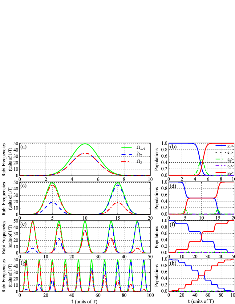
Figure 2: (Color online) Rabi frequencies (left column) and populations (left column) as s function of t for (from top to bottom) $N=1,2,5$, and $10$ pairs of pulses. Parameters used: $\Delta=350/T$.

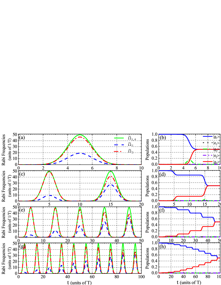
Figure 3: (Color online) Rabi frequencies (left column) and populations (left column) as s function of t for (from top to bottom) $N=1,2,5$, and $10$ pairs of pulses. Parameters used: $\Delta=350/T$.

Also, AE protocol ensures the decoupling of the excited states from the dynamics, we can directly move the population from state $|g_{1}\rangle$ to $|g_{3}\rangle$, $|e_{1}\rangle$ and $|e_{2}\rangle$ are only used to induce transitions but never significantly populated, as illustrated in Fig. 2. Thus the transfer process is insensitive to the properties of excited states, e.g., very short lifetime. This is very useful for depressing the effects of dissipation on the desired evolution of the system without relying on the dark state (9). Note that for $N\gg 1$ the total pulse area is very large, which is the condition for adiabatic evolution. This is useful when it is not possible to achieve high enough pulse areas needed for adiabatic evolution.

Fig. 3 shows the equal population distribution between $|g_{1}\rangle$ and $|g_{3}\rangle$. Similarly, the transient population of the intermediate state $|g_{2}\rangle$ is damped as $N(N=1,2,5,10)$ increases, and $|e_{1}\rangle$ and $|e_{2}\rangle$ are only used to induce transitions but never significantly populated. For this case, the analytic solution to maximum population in state $|g_{2}\rangle$ reads $P_{max}=\sin^{2}(\pi/8N)$. As $N$ tends to approach to infinity, the $P_{max}\approx(\pi/8N)^{2}$.

IV CONCLUSION

To conclude, we have generalized the coincident pulse technique in three-state system to a five-state chainwise system. With a train of $N(N\gg 1)$ pairs of coincident incident pulses, the present technique allows complete population transfer between initial state to final state, as well as the creation of arbitrary coherent superpositions of the initial and final states without significant population of the three intermediate states. The key of our protocol is reducing the M-type structure into a generalized $\Lambda$-type system with the simplest resonant coupling, the simplification is realized under the assumption of AE together with a requirement of the relation among the four incident pulses.

Finally, we believe that this technique is an interesting alternative of the existing techniques for coherent control of five-state chainwise systems. The results are of potential interest in applications where high-fidelity multi-state quantum control is essential, e.g., quantum information, atom optics, formation of ultracold molecules, cavity QED, nuclear coherent population transfer, light transfer in waveguide arrays, etc.

References

- Bergmann et al. (1998) K. Bergmann, H. Theuer, and B. W. Shore, Rev. Mod. Phys. 70, 1003 (1998).
- Vitanov et al. (2001a) N. V. Vitanov, T. Halfmann, B. W. Shore, and K. Bergmann, Annu. Rev. Phys. Chem. 52, 763 (2001a).
- Král et al. (2007) P. Král, I. Thanopulos, and M. Shapiro, Rev. Mod. Phys. 79, 53 (2007).
- Bergmann et al. (2015) K. Bergmann, N. V. Vitanov, and B. W. Shore, J. Chem. Phys. 142, 170901 (2015).
- Vitanov et al. (2017) N. V. Vitanov, A. A. Rangelov, B. W. Shore, and K. Bergmann, Rev. Mod. Phys. 89, 015006 (2017).
- Bergmann et al. (2019) K. Bergmann, H.-C. Nägerl, C. Panda, G. Gabrielse, E. Miloglyadov, M. Quack, G. Seyfang, G. Wichmann, S. Ospelkaus, A. Kuhn, S. Longhi, A. Szameit, P. Pirro, B. Hillebrands, X.-F. Zhu, J. Zhu, M. Drewsen, W. K. Hensinger, S. Weidt, T. Halfmann, H.-L. Wang, G. S. Paraoanu, N. V. Vitanov, J. Mompart, T. Busch, T. J. Barnum, D. D. Grimes, R. W. Field, M. G. Raizen, E. Narevicius, M. Auzinsh, D. Budker, A. Pálffy, and C. H. Keitel, J. Phys. B: At. Mol. Opt. Phys. 52, 202001 (2019).
- Vitanov (2020) N. V. Vitanov, Phys. Rev. A 102, 023515 (2020).
- Vitanov and Stenholm (1997) N. V. Vitanov and S. Stenholm, Phys. Rev. A 56, 1463 (1997).
- Wellnitz et al. (2020) D. Wellnitz, S. Schütz, S. Whitlock, J. Schachenmayer, and G. Pupillo, Phys. Rev. Lett. 125, 193201 (2020).
- Ciamei et al. (2017) A. Ciamei, A. Bayerle, C.-C. Chen, B. Pasquiou, and F. Schreck, Phys. Rev. A 96, 013406 (2017).
- Li et al. (2017) H. Li, H. Z. Shen, S. L. Wu, and X. X. Yi, Opt. Express 25, 30135 (2017).
- Zhang and Dou (2021) J.-H. Zhang and F.-Q. Dou, New J. Phys. 23, 063001 (2021).
- Stefanatos and Paspalakis (2021) D. Stefanatos and E. Paspalakis, Quantum Inf. Process. 20, 391 (2021).
- Zhang et al. (2023a) J.-H. Zhang, N. Naim, L. Deng, Y.-P. Niu, and S.-Q. Gong, Results Phys. 48, 106421 (2023a).
- Sola et al. (2018) I. R. Sola, B. Y. Chang, S. A. Malinovskaya, and V. S. Malinovsky, Adv. At. Mol. Opt. Phys. 67, 151 (2018).
- Vitanov et al. (2001b) N. Vitanov, M. Fleischhauer, B. Shore, and K. Bergmann, Adv. At. Mol. Opt. Phys. 46, 55 (2001b).
- Vitanov (1998a) N. V. Vitanov, Phys. Rev. A 58, 2295 (1998a).
- Oreg et al. (1992) J. Oreg, K. Bergmann, B. W. Shore, and S. Rosenwaks, Phys. Rev. A 45, 4888 (1992).
- Pillet et al. (1993) P. Pillet, C. Valentin, R.-L. Yuan, and J. Yu, Phys. Rev. A 48, 845 (1993).
- Malinovsky and Tannor (1997) V. S. Malinovsky and D. J. Tannor, Phys. Rev. A 56, 4929 (1997).
- Solá et al. (1999) I. R. Solá, V. S. Malinovsky, and D. J. Tannor, Phys. Rev. A 60, 3081 (1999).
- Linington et al. (2008) I. E. Linington, P. A. Ivanov, N. V. Vitanov, and M. B. Plenio, Phys. Rev. A 77, 063837 (2008).
- Grigoryan et al. (2015) G. Grigoryan, V. Chaltykyan, E. Gazazyan, O. Tikhova, and V. Paturyan, Phys. Rev. A 91, 023802 (2015).
- Kamsap et al. (2013) M. R. Kamsap, T. B. Ekogo, J. Pedregosa-Gutierrez, G. Hagel, M. Houssin, O. Morizot, M. Knoop, and C. Champenois, J. Phys. B: At. Mol. Opt. Phys. 46, 145502 (2013).
- Mukherjee et al. (2017) N. Mukherjee, W. E. Perreault, and R. N. Zare, J. Phys. B: At. Mol. Opt. Phys. 50, 144005 (2017).
- Sola et al. (2022) I. R. Sola, B. Y. Chang, S. A. Malinovskaya, S. C. Carrasco, and V. S. Malinovsky, J. Phys. B: At. Mol. Opt. Phys. 55, 234002 (2022).
- Theuer and Bergmann (1998) H. Theuer and K. Bergmann, Eur. Phys. J. D 2, 279 (1998).
- Goldner et al. (1994) L. S. Goldner, C. Gerz, R. J. C. Spreeuw, S. L. Rolston, C. I. Westbrook, W. D. Phillips, P. Marte, and P. Zoller, Phys. Rev. Lett. 72, 997 (1994).
- Parkins et al. (1993) A. S. Parkins, P. Marte, P. Zoller, and H. J. Kimble, Phys. Rev. Lett. 71, 3095 (1993).
- Parkins et al. (1995) A. S. Parkins, P. Marte, P. Zoller, O. Carnal, and H. J. Kimble, Phys. Rev. A 51, 1578 (1995).
- Simon et al. (2007) J. Simon, H. Tanji, S. Ghosh, and V. Vuletić, Nat. Phys. 3, 765 (2007).
- Danzl et al. (2010) J. G. Danzl, M. J. Mark, E. Haller, M. Gustavsson, R. Hart, J. Aldegunde, J. M. Hutson, and H.-C. Nägerl, Nat. Phys. 6, 265 (2010).
- Mark et al. (2009) M. J. Mark, J. G. Danzl, E. Haller, M. Gustavsson, N. Bouloufa, O. Dulieu, H. Salami, T. Bergeman, H. Ritsch, R. Hart, and H.-C. Nägerl, Appl. Phys. B 95, 219 (2009).
- Kuznetsova et al. (2008) E. Kuznetsova, P. Pellegrini, R. Côté, M. D. Lukin, and S. F. Yelin, Phys. Rev. A 78, 021402 (2008).
- Mackie and Phou (2010) M. Mackie and P. Phou, Phys. Rev. A 82, 011609R (2010).
- Qian et al. (2010) J. Qian, W. Zhang, and H. Y. Ling, Phys. Rev. A 81, 013632 (2010).
- Price and Yelin (2019) P. Price and S. F. Yelin, Phys. Rev. A 100, 033421 (2019).
- Hutson (2010) J. M. Hutson, Science 327, 788 (2010).
- Ulmanis et al. (2012) J. Ulmanis, J. Deiglmayr, M. Repp, R. Wester, and M. Weidemüller, Chem. Rev. 112, 4890 (2012).
- Carr et al. (2009) L. D. Carr, D. DeMille, R. V. Krems, and J. Ye, New J. Phys. 11, 055049 (2009).
- Amiri and Saadati-Niari (2023) M. Amiri and M. Saadati-Niari, Phys. Scr. 98, 085303 (2023).
- Liao et al. (2011) W.-T. Liao, A. Pálffy, and C. H. Keitel, Phys. Lett. B 705, 134 (2011).
- Liao et al. (2013) W.-T. Liao, A. Pálffy, and C. H. Keitel, Phys. Rev. C 87, 054609 (2013).
- Kirschbaum et al. (2022) T. Kirschbaum, N. Minkov, and A. Pálffy, Phys. Rev. C 105, 064313 (2022).
- Seiferle et al. (2019) B. Seiferle, L. von der Wense, P. V. Bilous, I. Amersdorffer, C. Lemell, F. Libisch, S. Stellmer, T. Schumm, C. E. Düllmann, A. Pálffy, and P. G. Thirolf, Nature 573, 243 (2019).
- Della Valle et al. (2008) G. Della Valle, M. Ornigotti, T. Toney Fernandez, P. Laporta, S. Longhi, A. Coppa, and V. Foglietti, Appl. Phys. Lett. 92, 011106 (2008).
- Tseng and Wu (2010) S.-Y. Tseng and M.-C. Wu, J. Lightwave Technol. 28, 3529 (2010).
- Ciret et al. (2013) C. Ciret, V. Coda, A. A. Rangelov, D. N. Neshev, and G. Montemezzani, Phys. Rev. A 87, 013806 (2013).
- N. Irani and Saadati-Niari (2022) M. A.-T. N. Irani and M. Saadati-Niari, J. Mod. Opt 69, 12 (2022).
- Zhang et al. (2023b) J.-H. Zhang, L. Deng, Y.-P. Niu, and S.-Q. Gong, (2023b), arXiv:2310.11071 [quant-ph] .
- Rangelov and Vitanov (2012) A. A. Rangelov and N. V. Vitanov, Phys. Rev. A 85, 043407 (2012).
- Nedaee-Shakarab et al. (2016) B. Nedaee-Shakarab, M. Saadati-Niari, and F. Zolfagharpour, Phys. Rev. C 94, 054601 (2016).
- Nedaee-Shakarab et al. (2017) B. Nedaee-Shakarab, M. Saadati-Niari, and F. Zolfagharpour, Phys. Rev. C 96, 044619 (2017).
- Wang et al. (2012) H. Wang, Y.-M. Liu, J.-W. Gao, D. Yan, R. Wang, and J.-H. Wu, Opt. Commun. 285, 3498 (2012).
- Zhang et al. (2015) Y. Zhang, Y.-M. Liu, X.-D. Tian, T.-Y. Zheng, and J.-H. Wu, Phys. Rev. A 91, 013826 (2015).
- Huang et al. (2014) W. Huang, A. A. Rangelov, and E. Kyoseva, Phys. Rev. A 90, 053837 (2014).
- Alrifai et al. (2021) R. Alrifai, V. Coda, J. Peltier, A. A. Rangelov, and G. Montemezzani, Phys. Rev. A 103, 023527 (2021).
- Vitanov (1998b) N. V. Vitanov, J. Phys. B: At. Mol. Opt. Phys. Mol. Opt. Phys. 31, 709 (1998b).
- Zhang (2023) J. Zhang, (2023), arXiv:2311.05951 [physics.optics] .
- Shore et al. (1991) B. W. Shore, K. Bergmann, J. Oreg, and S. Rosenwaks, Phys. Rev. A 44, 7442 (1991).