Discretization of continuous-time arbitrage strategies in financial markets with fractional Brownian motion

Abstract

This study evaluates the practical usefulness of continuous-time arbitrage strategies designed to exploit serial correlation in fractional financial markets. Specifically, we revisit the strategies of Shiryaev (1998) and Salopek (1998) and transfer them to a real-world setting by distretizing their dynamics and introducing transaction costs. In Monte Carlo simulations with various market and trading parameter settings, we show that both are highly promising with respect to terminal portfolio values and loss probabilities. These features and complementary sparsity make them valuable additions to the toolkit of quantitative investors.

1 Introduction

Motivated by the challenge they pose to the traditional notion of efficient capital markets, financial research has intensively studied investment strategies which solely rely on past asset price information. Among the most prominent studies, Jegadeesh and Titman (1993, 2001) have shown that cross-sectional momentum, i.e., buying past winners and selling past losers, is highly beneficial. In addition, Moskowitz et al. (2012) identify a time-series momentum effect according to which single assets exhibit exploitable trending behavior. What these strategies have in common is that their profitability is linked to a positive serial correlation in asset price movements (see Pan et al., 2004; Hong and Satchell, 2015).

Even though momentum investing has become a standard in the mutual fund industry (see Barroso and Santa-Clara, 2015), financial research and practice has paid surprisingly little attention to a very interesting strand of mathematical literature developing arbitrage strategies for assets with serially correlated returns. It is well known that pure arbitrage, i.e., the realization of risk-less profits from zero initial investment, is impossible in a traditional Black-Scholes market with standard Brownian motion (sBm). In contrast, arbitrage opportunities can arise in markets where asset prices are driven by a fractional Brownian motion (fBm) which dates back to Mandelbrot and Ness (1968) and superimposes memory features on asset returns. In a continuous-time setup with slowly decaying positive serial correlation, i.e., the fractional Black-Scholes model of Cutland et al. (1995), the theoretical studies of Shiryaev (1998) and Salopek (1998) show that risk-less profits can be earned by buying high-priced and short-selling low-priced assets in adequate numbers. Bayraktar and Poor (2005) extend the work of Shiryaev (1998) by incorporating stochastic volatility. Rogers (1997) and Cheridito (2003) develop additional but more complex strategies.

While the simplicity of the Shiryaev and Salopek arbitrage strategies and empirical evidence on memory in equity, futures and fund returns (see Wang et al., 2012; Di Cesare et al., 2015; Coakley et al., 2016) make them highly appealing for investment practice, they are built on the premise of continuous-time trading with no frictions. Cheridito (2003) and Guasoni (2006) highlight that, in a fractional Black-Scholes world, arbitrage opportunities vanish with the introduction of a minimal waiting time between subsequent transactions, i.e., discrete-time trading, and proportional transaction costs of any positive size, respectively. However, this does not necessarily mean that the above strategies should be discarded. When suitably discretized and parameterized, they may not be entirely self-financing and risk-free, but still provide positive expected payoffs at a low risk of loss. In other words, they could share some valuable properties with statistical arbitrage strategies (see Bondarenko, 2003; Lütkebohmert and Sester, 2019).

After exploring the properties and the economic intuition of the Shiryaev and Salopek strategies, the core objective of our study is to investigate their investment performance in a real-world setting. This means that, in a first step, we discretize the strategies and install different forms of transaction costs. This is not trivial because discretization alone makes the strategies lose their self-financing property and requires suitable countermeasures to maintain tradeability. In a second step, we perform an extensive Monte Carlo study for the discretized versions of the strategies. Here, we are particularly interested in whether they deliver positive terminal portfolio values on average and display acceptably small loss probabilities. We focus on these two quantities because they are central to established arbitrage definitions and allow a modern downside-oriented investment evaluation (see Eling and Schuhmacher, 2007; Cumova and Nawrocki, 2014). To answer our research question, we use the spectral method of Yin (1996) for fBm simulation which, in contrast to alternatives, preserves the basic features of fBms (see Kijima and Tam, 2013). We analyze the strategies with asset and trading parameters tailored to the current market environment exhibiting, for example, significantly falling transaction costs (see Chordia et al., 2014). Furthermore, we conduct a variety of sensitivity checks to identify the situations in which they perform best and worst. Overall, this results in an intuitive guide on how to chose, for example, the ideal candidate assets, parameters and trading frequencies of the strategies.

The remainder of our study is organized as follows. Section 2 introduces the fractional Black-Scholes model, discusses the corresponding Shiryaev and Salopek arbitrage strategies and translates them to a discrete-time setting with transaction costs. Section 3 presents our Monte Carlo study examining the impact of discretization, transaction costs, model parameters as well as trading horizon and frequency on the strategies. Section 4 concludes and outlines directions for future research.

2 Theoretical framework

2.1 Continuous-time market setup

We start our analysis by specifying the asset price behavior in a fractional Black-Scholes model and explain how self-financing portfolios are formed in such an environment.

Asset prices

For a fixed date or investment horizon $T>0$, we consider a filtered probability space $(\Omega,\pazocal{F},\mathbb{F},\mathbb{P})$ with standard filtration $\mathbb{F}=(\pazocal{F}_{t})_{t\in[0,T]}$ and assume that all processes are $\mathbb{F}$-adapted. In this context, the fractional Black-Scholes model suggests that we have one risk-free asset with constant price $S^{0}_{t}=1$ and $d$ risky assets with a price process $S=(S^{1},\ldots,S^{d})$ defined on $[0,T]$ by the stochastic differential equations (SDEs)

$$dS_{t}^{i}=\mu^{i}S_{t}^{i}dt+\sigma^{i}S_{t}^{i}dB_{t}^{H^{i}},\quad S_{0}^{i}=s_{0}^{i},\quad i=1,\ldots,d.$$ (2.1)

Here, the drifts or expected returns $\mu^{i}\in\mathbb{R}$, volatilities $\sigma^{i}>0$ and initial prices $s_{0}^{i}>0$ are given constants. In contrast to the standard Black-Scholes model, the SDEs are not driven by sBms (or Wiener processes) but by fBms $B_{t}^{H^{i}}$ with Hurst parameters $H^{i}\in(0.5,1)$. The fBms are assumed to be independent, which is reasonable when the risky assets are, for example, certain types of industry portfolios, investment funds or commodity futures baskets (see Erb and Harvey, 2006; Badrinath and Gubellini, 2011).

The one-dimensional fBm $(B_{t}^{H})_{t\in[0,T]}$ is a centered Gaussian process with covariance

$$\textrm{Cov}(B_{t}^{H},B_{s}^{H})=\frac{1}{2}\left(|t|^{2H}+|s|^{2H}-|t-s|^{2H}\right)\quad\text{for}\quad H\in(0,1).$$ (2.2)

It is a self-similar process with stationary increments. The special case $H=0.5$ reflects the sBm which has independent increments and enjoys the martingale property. For $H\neq 0.5$, the increments are correlated and the process is not a martingale. This implies memory effects for the asset returns $dS^{i}_{t}/S^{i}_{t}$. For the range $H\in(0.5,1)$ considered in the fractional Black-Scholes world, asset returns are positively correlated, i.e., persistent. While, for $H=0.5$, we have to rely on Itô’s calculus, $H>0.5$ allows us to define stochastic integrals w.r.t. $B_{t}^{H}$ path-wise in the Riemann-Stieltjes sense (see Sottinen and Valkeila, 2003). Thus, the solutions of the SDEs in (2.1) are

$$S_{t}^{i}=s_{0}^{i}\,\exp\big{\{}\mu^{i}t+\sigma^{i}B_{t}^{H^{i}}\big{\}},\quad t\in\left[0,T\right].$$ (2.3)

The processes defined in (2.3) are called geometric fBms.

Portfolios

Asset transactions in a fractional Black-Scholes market are modeled based on the usual assumptions of permanent trading, unlimited borrowing and short-selling, real asset quantities and contemporary agreement of buying and selling prices. Furthermore, there are no transaction costs, fees or taxes. We can describe the trading activity of an investor by an initial amount of capital $v\in\mathbb{R}$ and a $\mathbb{F}$-adapted process

$$\Psi=(\Psi_{t})_{t\in\left[0,T\right]}=(\Psi_{t}^{0},\Psi_{t}^{1},\ldots,\Psi_{t}^{d})_{t\in\left[0,T\right]}.$$ (2.4)

Here, $\Psi_{t}^{0}\in\mathbb{R}$ and $\Psi_{t}^{1},\ldots,\Psi_{t}^{d}\in\mathbb{R}$ denote the numbers of risk-free and risky assets held by the investor at time $t$, respectively. $\Psi$ is called portfolio or trading strategy. The investor has a long (short) position if $\Psi_{t}^{i},i=0,\ldots,d,$ is positive (negative). At time $t$, the value $V_{t}^{\Psi}$ of the portfolio $\Psi$ is given by

$$V_{t}^{\Psi}=\sum_{i=0}^{d}\Psi_{t}^{i}S_{t}^{i}.$$ (2.5)

$V^{\Psi}=(V_{t}^{\Psi})_{t\in[0,T]}$ is the value process of $\Psi$. In an arbitrage context, $\Psi$ is assumed to be self-financing. This means that there is no exogenous infusion or withdrawal of capital after the purchase of the portfolio. Rebalancing the portfolio must be financed solely by trading the $d+1$ available assets. Mathematically, self-financing in a continuous-time market is defined by the property that the value process for all $t\in[0,T]$ can be expressed as

$$V_{t}^{\Psi}=v+G_{t}^{\Psi}\quad\text{where }~{}~{}G_{t}^{\Psi}=\sum_{i=0}^{d}\int_{0}^{t}\Psi_{s}^{i}dS^{i}_{s}.$$ (2.6)

$G^{\Psi}=(G_{t}^{\Psi})_{t\in[0,T]}$ is the gain process of $\Psi$, where the gain $G_{t}^{\Psi}$ at time $t$ is given by a sum of stochastic integrals w.r.t. geometric fBms (see Salopek, 1998). The self-financing condition (2.6) can also be stated in differential form, i.e., $dV_{t}^{\Psi}=\sum_{i=0}^{d}\Psi_{s}^{i}dS^{i}_{s}$. It shows that, for a self-financing strategy, the changes in portfolio value are not due to rebalancing but rather to changes in asset prices.

2.2 Continuous-time arbitrage

In a standard Black-Scholes world, arbitrage is impossible. This is a consequence of the fundamental theorem of asset pricing (see Delbaen and Schachermayer, 1994; Björk, 2004) and has its roots in the sBm martingale property. In contrast, a fBm with $H\neq 0.5$ behaves predictably such that our fractional Black-Scholes world offers arbitrage opportunities which can be exploited by constructing suitable arbitrage portfolios. A self-financing portfolio $\Psi$ is called an arbitrage portfolio if its value process satisfies the three properties

(i) $$V_{0}^{\Psi}=0,$$ (2.7)

(ii) $$\mathbb{P}(V_{t}^{\Psi}\geq 0\text{ for all }t\in(0,T])=1,$$

(iii) $$\mathbb{P}(V_{T}^{\Psi}>0)>0.$$

This implies that arbitrage is essentially the possibility to generate a positive amount of money without having to invest any initial capital and without any risk of loss. In the following, we present two simple arbitrage strategies satisfying the properties in (2.7).

Remark 2.1

For every arbitrage strategy $\Psi$, the scaled strategy $\widetilde{\Psi}=\gamma\Psi$ with $\gamma>0$ is also an arbitrage strategy. This is because (2.5) and (2.6) imply $V^{\widetilde{\Psi}}=\gamma V^{\Psi}$ and $G^{\widetilde{\Psi}}=\gamma G^{\Psi}$, respectively. Since the initial value $V^{\Psi}_{0}$ is zero, we also have $V^{\widetilde{\Psi}}_{0}=0$. Hence, $\widetilde{\Psi}$ satisfies the self-financing condition $V_{t}^{\widetilde{\Psi}}=v+G_{t}^{\widetilde{\Psi}}$ in (2.6) with $v=0$. Finally, $V^{\widetilde{\Psi}}=\gamma V^{\Psi}$ implies that $\widetilde{\Psi}$ fulfills the arbitrage conditions in (2.7).

Shiryaev strategy

Shiryaev (1998) proposes a strategy that generates an arbitrage portfolio consisting of the risk-free asset and one risky asset. Thus, we have $d=1$. For simplicity, we denote the drift, volatility and Hurst coefficient of the risky asset by $\mu$, $\sigma$ and $H$, respectively. For the two assets, the strategy suggests entering the time $t\in[0,T]$ positions

$$\begin{array}[]{rcccl}\Psi_{t}^{0}&=&\frac{1}{s_{0}^{1}}\big{(}{(s_{0}^{1}})^{2}-(S_{t}^{1})^{2}\big{)}&=&s_{0}^{1}\big{(}1-\exp\big{\{}{2\mu t+2\sigma B_{t}^{H}}\big{\}}\big{)},\\[4.30554pt] \Psi_{t}^{1}&=&\frac{2}{s_{0}^{1}}({S_{t}^{1}}-{s_{0}^{1}})&=&2\big{(}\exp\big{\{}\mu{t}+\sigma B_{t}^{H}\}-1\big{)}.\end{array}$$ (2.10)

At every $t$, it compares the value $S_{t}^{1}$ of a pure risky investment with an alternative investment of the initial risky asset price $s_{0}^{1}$ in the risk-free asset. Because, in our market model, we have $S_{t}^{0}=1$, this alternative investment has a constant value of $s_{0}^{1}$. If the value $S_{t}^{1}$ of the pure risky investment exceeds (falls below) the value $s_{0}^{1}$ of the alternative investment, the investor holds a long (short) position in the risky asset and a short (long) position in the risk-free asset. In the case of equality, he is not invested and the portfolio value is zero. The number of risky asset shares $\Psi_{t}^{1}$ in (2.10) does not depend on the initial risky asset price $s_{0}^{1}$ but on the parameters $\mu$, $\sigma$ and $H$.

Shiryaev (1998) shows that the strategy $\Psi$ in (2.10) is self-financing. Furthermore, at time $t=0$, we have $\Psi_{0}^{0}=\Psi_{0}^{1}=0$ and hence $V_{0}^{\Psi}=0$, i.e., no initial investment is required. Substituting (2.10) into (2.5) shows that the portfolio value at any time $t\in[0,T]$ is

$$V^{\Psi}_{t}=(S_{t}^{1}-s_{0}^{1})^{2}/s_{0}^{1}\geq 0.$$ (2.11)

We obtain $\mathbb{P}(V_{T}^{\Psi}>0)>0$. Thus, according to (2.7), $\Psi$ is indeed an arbitrage strategy.

Salopek strategy

Another arbitrage strategy, dating back to Harrison et al. (1984) and applied in a fractional Black-Scholes market by Salopek (1998), trades $d\geq 2$ risky assets and ignores the risk-free asset. It is defined for two real-valued constants $\alpha<\beta$ and can be summarized as $\Psi=(0,\Psi(\alpha,\beta))$ or, with some abuse of notation, $\Psi=\Psi(\alpha,\beta)$. The entries of $\Psi(\alpha,\beta)=(\Psi_{t}^{1}(\alpha,\beta),\ldots,\Psi_{t}^{d}(\alpha,\beta))$ are the risky asset shares at time $t\in[0,T]$. Specifically, for $i=1,\ldots,d$, we have

$$\Psi_{t}^{i}(\alpha,\beta)=\widehat{\Psi}_{t}^{i}(\beta)-\widehat{\Psi}_{t}^{i}(\alpha),\quad\text{where }\quad\widehat{\Psi}_{t}^{i}(a)=\frac{1}{d}\left(\frac{S_{t}^{i}}{M_{a}(S_{t})}\right)^{a-1}.$$ (2.12)

$M_{a}(x)$ denotes the $a$-order power mean of $x=(x^{1},\ldots,x^{d})\in\mathbb{R}_{+}^{d}$. It is given by

$$M_{a}(x)=\Big{(}\frac{1}{d}\sum_{i=1}^{d}(x^{i})^{a}\Big{)}^{1/a} \quad a\neq 0,$$ for (2.13)

$$M_{0}(x)=\sqrt[d]{x^{1}\cdot\ldots\cdot x^{d}} \quad a=0.$$ for

To provide an economic interpretation of this strategy, it is instructive to recall some properties of the involved family of power means (see Hardy et al., 1934).

Remark 2.2

With respect to the properties of the $a$-order power mean, we can list the following important special cases:

$$\begin{array}[]{lll}M_{1}(x)&=(x^{1}+\ldots+x^{d})/d&\qquad(\text{arithmetic mean})\\[2.15277pt] M_{2}(x)&=\sqrt{((x^{1})^{2}+\ldots+(x^{d})^{2})/d}&\qquad(\text{quadratic mean})\\[2.15277pt] M_{-1}(x)&=\big{(}(1/x^{1}+\ldots+1/x^{d})/d\big{)}^{-1}&\qquad(\text{harmonic mean})\\[2.15277pt] M_{0}(x)&=\sqrt[d]{x^{1}\cdot\ldots\cdot x^{d}}=\lim_{a\to 0}M_{a}(x)&\qquad(\text{geometric mean})\\[2.15277pt] M_{\infty}(x)&:=\lim_{a\to+\infty}M_{a}(x)=x_{max}=\max\{x^{1},\ldots,x^{d}\}&\qquad(\text{maximum of }x)\\[2.15277pt] M_{-\infty}(x)&:=\lim_{a\to-\infty}M_{a}(x)=x_{min}=\;\min\{x^{1},\ldots,x^{d}\}&\qquad(\text{minimum of }x)\\ \end{array}$$

Furthermore, the function $a\mapsto M_{a}(x)$ is increasing. For $a<b$, we have

$$x_{min}\leq M_{a}(x)\leq M_{b}(x)\leq x_{max}$$ (2.14)

with equalities if and only if $x^{1}=\ldots=x^{d}=\overline{x}$, i.e., all entries of $x$ are identical. In this situation, $M_{a}(x)=\overline{x}$ holds for all $a\in\mathbb{R}$.

The strategy $\Psi(\alpha,\beta)$ in (2.12) is expressed as the difference between $\widehat{\Psi}(\beta)$ and $\widehat{\Psi}(\alpha)$. Because these two components can be considered as strategies themselves, we call $\widehat{\Psi}(a)$ an $a$-strategy or $a$-portfolio. Consequently, an investor can implement $\Psi(\alpha,\beta)$ by purchasing a $\beta$-portfolio and short-selling an $\alpha$-portfolio.

Substituting the $\widehat{\Psi}(a)$ specified by (2.12) into (2.5) provides the portfolio value of an $a$-strategy, i.e., we obtain

$$V_{t}^{\widehat{\Psi}(a)}=M_{a}(S_{t}).$$ (2.15)

It also shows that $V_{0}^{\widehat{\Psi}(a)}=M_{a}(s_{0})$, i.e., the initial investment is positive and equals the $a$-order power mean of initial asset prices $s_{0}$. An $a$-strategy investor enters long positions in all $d$ risky assets and chooses their numbers proportional to $(S_{i}^{t})^{a-1}$. More specifically, for $a=1$, we have $\widehat{\Psi}_{t}^{i}=1/d$, i.e., an equally allocated investment, and the portfolio value is $V_{t}^{\widehat{\Psi}(1)}=M_{1}(S_{t})$, i.e., the arithmetic mean of prices. For $a>1$ ($a<1$), the portfolio contains more (fewer) high-priced assets than low-priced assets. This feature becomes more pronounced with higher (lower) orders $a>1$ ($a<1$). In the limit for $a\to\infty$ ($a\to-\infty$), the investor only holds the asset with the highest (lowest) price. If there are $m\geq 1$ risky assets sharing this price, he orders $1/m$ each.

The strategy (2.12) is an arbitrage strategy if we impose the following assumption to the financial market model.

Assumption 2.3

All price processes $(S_{t}^{i})_{t\in[0,T]}$ of the risky assets $i=1,\ldots,d$ start at time $t=0$ with identical initial prices $S_{0}^{i}=\widetilde{s}>0$.

Remark 2.4

Assumption 2.3 serves mathematical simplification and will not be fulfilled in practice. However, this is not problematic because we can rescale the asset prices via $\widetilde{S}_{t}^{i}=\frac{\widetilde{s}}{s_{0}^{i}}S_{t}^{i}$ to $\widetilde{S}_{0}^{i}=\widetilde{s}$ and compute the arbitrage positions $\widetilde{\Psi}_{t}^{i}$ in the rescaled market. They are linked to the original market via $\Psi_{t}^{i}=\frac{\widetilde{s}}{s_{0}^{i}}\widetilde{\Psi}_{t}^{i}$. Because $\Psi_{t}^{i}S_{t}^{i}=\widetilde{\Psi}_{t}^{i}\widetilde{S}_{t}^{i}$, (2.5) delivers $V^{\Psi}_{t}=V^{\widetilde{\Psi}}_{t}$. That is, the portfolio value is not affected by the transformation.

We now show that (2.12) satisfies the three conditions in (2.7) and is in fact an arbitrage strategy. As far as the self-financing property is concerned, it has been verified by Salopek (1998). According to (2.15), for all $t\in[0,T]$, the portfolio value is given by

$$V_{t}^{\Psi}=V_{t}^{\widehat{\Psi}(\beta)}-V_{t}^{\widehat{\Psi}(\alpha)}=M_{\beta}(S_{t})-M_{\alpha}(S_{t})\geq 0,$$ (2.16)

where we have used the assumption $\alpha<\beta$ and relation (2.14) stating that $M_{a}(\cdot)$ is increasing in $a$. This proves condition (ii) in (2.7). Condition (i) on zero initial investment follows from Assumption 2.3 of identical initial asset prices. It yields $V_{0}^{\Psi}=M_{\beta}(s_{0})-M_{\alpha}(s_{0})=\widetilde{s}-\widetilde{s}=0$. Finally, because we have assumed that the asset prices (2.1) are driven by independent fBms, prices are uncorrelated and thus, at time $T$, almost surely not identical. This implies the strict inequality $V_{T}^{\Psi}=M_{\beta}(S_{T})-M_{\alpha}(S_{T})>0$ with probability one such that arbitrage condition (iii) is also satisfied.

The monotonicity property (2.14) of the $a$-order power mean and the portfolio value expression (2.16) suggest to choose the largest possible $\beta$ and the smallest possible $\alpha$. Fusing the limits $\beta\to\infty$ and $\alpha\to-\infty$ into the following proposition shows that an arbitrage strategy with large $d$ can reduce to just buying the asset $i$ with the highest price and short-selling the asset $j$ with the lowest price.

Proposition 2.1

Let $i,j\in\{1,...,d\}$, $t\in[0,T]$ and $\alpha<1\leq\beta$ such that prices satisfy

$$S_{t}^{i}>M_{\beta}(S_{t})>M_{\alpha}(S_{t})>S_{t}^{j}.$$ (2.17)

Then, the strategy (2.12) has the property $\Psi_{t}^{i}(\alpha,\beta)>0>\Psi_{t}^{j}(\alpha,\beta)$. That is, the investor buys the high-priced $i$ and short-sells the low-priced $j$. This particularly holds when the prices of $i$ and $j$ represent the maximum and minimum over all $S_{t}^{1},\ldots,S_{t}^{d}$.

Proof

See Appendix A.

2.3 Discrete-time arbitrage

We now replace the idealized continuous-time financial market model with permanent and frictionless asset transfers by a more realistic setup where trading takes place only at a finite number of fixed points in time and is subject to transaction costs.

Discrete-time trading

In the discrete-time financial market model, prices are quoted at the times $0=t_{0}<t_{1}<\ldots<t_{N}=T$. A portfolio is created at time $t_{0}=0$, rebalanced at times $t_{1},\ldots,t_{N-1}$ and liquidated at terminal time $t_{N}=T$. We focus on equidistant instants of time $t_{n}=nT/N,n=0,\ldots,N$, which divide the total trading horizon $[0,T]$ into $N$ trading periods of the same length $T/N$. Thus, sampling the asset price processes (2.3) of the fractional Black-Scholes model at $t_{0},\ldots,t_{N}$ generates a sequence of risk-free asset prices $\left(S_{t_{n}}^{0}\right)_{n=0,...,N}$ and $d$ sequences of risky asset prices $\left(S_{t_{n}}^{i}\right)_{n=0,...,N}$ defined by

$$S_{t_{n}}^{0}=1,\quad S_{t_{n}}^{i}=s_{0}^{i}\exp\big{\{}\mu^{i}t_{n}+\sigma^{i}B_{t_{n}}^{H^{i}}\},\quad\text{for}\quad n=0,\ldots,N\text{ and }i=1,\ldots,d,$$ (2.18)

with the same parameters as in Section 2.1.

It has to be expected that the discretization of a self-financing continuous-time strategy $\Psi$, such as the Shiryaev and Salopek strategies of Section 2.2, and the existence of transaction costs affect the self-financing property. Even without transaction costs, rebalancing a portfolio according to a discretized self-financing continuous-time strategy requires the infusion of or allows the withdrawal of capital. These rebalancing costs and the classic transaction costs may be incorporated by modifying the risk-free asset holdings $\Phi^{0}$ defined below. However, because we wish to explicitly quantify the impact of time discretization and transaction costs on continuous-time arbitrage strategies, we extend our financial market model by an additional asset $d+1$ which we call transaction account. In the investment fund industry, such (cash) accounts are used to react flexibly to market events (see Nascimento and Powell, 2010; Simutin, 2014). In our context, it allows us to express the aforementioned impact in monetary units. Similar to the risk-free asset price $S^{0}$, the price process of the new asset is a constant process $S^{d+1}=(S^{d+1}_{t_{n}})_{n=0,\ldots,N}$ with $S^{d+1}_{t_{n}}=1$.

We capture the trading activity of an investor by an initial capital amount $v\in\mathbb{R}$ and the discrete-time $\mathbb{F}$-predictable process

$$\Phi=(\Phi_{n})_{n=1,\ldots,N+1}=(\Phi_{n}^{0},\Phi_{n}^{1},\ldots,\Phi_{n}^{d+1})_{n=1,\ldots,N+1}.$$ (2.19)

Here, $\Phi_{n}^{0}$ and $\Phi_{n}^{d+1}\in\mathbb{R}$ denote for $n=1,...,N$ the holdings in the risk-free asset and the transaction account, respectively, chosen at the beginning of the $n$-th trading period $[t_{n-1},t_{n})$ and kept constant over that period. Further, $\Phi_{n}^{i}\in\mathbb{R}$ is the quantity of risky asset $i=1,\ldots,d$ held in the $n$-th trading period. The vector $\Phi_{N+1}$ relates to the liquidation of the portfolio at time $t_{N}=T$. Overall, $\Phi$ is the discrete-time portfolio or trading strategy.

Discretizing the continuous-time strategy $\Psi=(\Psi_{t})_{t\in[0,T]}$ in (2.4) leads to a piece-wise constant strategy where the investor period-wise sets and upholds $\Psi$. This means that, for $i=0,\ldots,d$, we have $\Phi_{n}^{i}=\Psi_{t_{n-1}}^{i},n=1,\ldots,N$, whereas liquidating the portfolio yields $\Phi_{N+1}^{i}=0$. The positions $\Phi_{n}^{d+1}$ in the transaction account are specified in what follows.

Transaction costs

For purchasing, rebalancing and liquidating the portfolio, the investor has to pay transaction costs depending on the trading volume of the risky assets. For a given strategy $\Phi$, at time $t$, this volume is defined by

$$\Gamma^{\Phi}_{t}=\left\{\begin{array}[]{{lll}}\sum_{i=1}^{d}\left|\Phi_{1}^{i}\right|S_{0}^{i},&t=t_{0}=0,&\text{(purchasing)}\\[4.30554pt] \sum_{i=1}^{d}\left|\Phi_{n+1}^{i}-\Phi_{n}^{i}\right|S_{t_{n}}^{i},&t=t_{1},\ldots,t_{N-1},&\text{(rebalancing)}\\[4.30554pt] \sum_{i=1}^{d}\left|\Phi_{N}^{i}\right|S_{T}^{i},&t=t_{N}=T.&\text{(liquidating)}\\ \end{array}\right.$$ (2.23)

We specify transaction costs proportional to the trading volume. They are determined by the proportionality factor $p_{1}\geq 0$ (in percent) if they exceed the minimum fee $p_{2}\geq 0$ (in monetary units). Otherwise, $p_{2}$ is charged. We denote $p=(p_{1},p_{2})$ and define the transaction costs for $t=t_{0},\ldots,t_{N}$ as

$$L_{t}^{\Phi}=l(\Gamma^{\Phi}_{t},p)\quad\text{with}\quad l(y,p)=\max(p_{1}y,p_{2})\mathbbm{1}_{\{y>0\}}.$$ (2.24)

Note that no transaction costs are charged at time $t$ if the trading volume $\Gamma^{\Phi}_{t}$ is zero. The special case of a model without transaction costs is reflected by $p_{1}=p_{2}=0$.

Liquidation

In the continuous-time model with frictionless trading, the terminal portfolio value $V_{T}^{\Psi}$ in (2.5) is equal to the revenue from selling the portfolio. In the discrete-time case, liquidating the portfolio induces the transaction costs $L^{\Phi}_{t_{N}}=l(\Gamma^{\Phi}_{t_{N}},p)$ of (2.23) and (2.24). Thus, the net revenue is

$$R^{\Phi}=\sum_{i=0}^{d}\Phi_{N}^{i}S_{T}^{i}-L_{T}^{\Phi}.$$ (2.25)

Transaction account

As discussed above, we have augmented our model by an asset $d+1$ called transaction account. It is used to finance rebalancing and transaction costs. Furthermore, it receives the net liquidation revenue at terminal time $t_{N}=T$. We now derive the holdings $\Phi^{d+1}_{n},n=1,\ldots,N+1$, for this asset. To this end, the rebalancing costs of a strategy $\Phi$ at time $t_{n}$ are denoted by $D_{t_{n}}^{\Phi}$ and defined as the value difference between the (risk-free and risky) asset holdings after and before trading:

$$D_{t_{n}}^{\Phi}=\sum\limits_{i=0}^{d}\Phi_{n+1}^{i}S_{t_{n}}^{i}-\sum\limits_{i=0}^{d}\Phi_{n}^{i}S_{t_{n}}^{i} =\sum\limits_{i=0}^{d}\big{(}\Phi_{n+1}^{i}-\Phi_{n}^{i}\big{)}S_{t_{n}}^{i}$$ (2.26)

$$=\sum\limits_{i=0}^{d}\big{(}\Psi_{t_{n}}^{i}-\Psi_{t_{n-1}}^{i}\big{)}S_{t_{n}}^{i},~{}n=1,\ldots,N-1.$$

Here, the last line follows from the sampling property $\Phi_{n}^{i}=\Psi_{t_{n-1}}^{i},i=1,\ldots,d$. Also note that the rebalancing costs at time $t_{0}=0$ and $t_{N}=T$ are zero.

Aggregating the rebalancing and transaction costs as well as the net liquidation revenue, the holdings in the transaction account can be stated recursively by

$${\Phi}_{1}^{d+1} =-L_{0}^{\Phi}, (\text{purchasing})$$

$${\Phi}_{n+1}^{d+1} ={\Phi}_{n}^{d+1}-D_{t_{n}}^{\Phi}-L_{t_{n}}^{\Phi},\quad n=1,\ldots,N-1, (\text{rebalancing})$$ (2.27)

$${\Phi}_{N+1}^{d+1} ={\Phi}_{N}^{d+1}+R^{\Phi}, (\text{liquidating})$$

where $L_{t}^{\Phi}$, $R^{\Phi}$ and $D_{t}^{\Phi}$ are obtained according to (2.24), (2.25) and (2.26), respectively.

Portfolio value

At time $t_{n}$, the value $V_{t_{n}}^{\Phi}$ of the portfolio $\Phi$ is

$$V_{t_{n}}^{\Phi}=\sum_{i=0}^{d+1}\Phi_{n+1}^{i}S_{t_{n}}^{i},\quad n=0,\ldots,N.$$ (2.28)

$V^{\Phi}=(V_{t_{n}}^{\Phi})_{n=0,\ldots,N}$ is the discrete-time value process. While, at time $t=0$, the continuous-time model yields $V_{t_{0}}^{\Psi}=v$, the discrete-time case delivers $V_{0}^{\Phi}=v-L_{0}^{\Phi}$. That is, the portfolio value equals the initial capital minus the transaction costs for purchasing the portfolio. If $\Phi$ results from discretizing a continuous-time arbitrage strategy $\Psi$ with $V_{0}^{\Psi}=v=0$, the discrete-time value process starts with $V_{0}^{\Phi}=-L_{0}^{\Phi}\leq 0$. This term is strictly negative if the initial trading volume $\Gamma_{0}^{\Phi}$ and at least one of the two transaction cost parameters $p_{1}$ and $p_{2}$ is positive. For the terminal trading time $t_{N}=T$, substituting $\Phi^{0}_{N+1}=\ldots=\Phi^{d}_{N+1}=0$ into (2.28) and applying (2.27) provides $V_{T}^{\Phi}=\Phi_{N+1}^{d+1}S_{t_{n}}^{d+1}={\Phi}_{N}^{d+1}+R^{\Phi}$. Hence, the terminal portfolio value equals the net liquidation revenue $R^{\Phi}$ minus the accumulated rebalancing and transaction costs ${\Phi}_{N}^{d+1}$ for trading at times $t_{0},\ldots,t_{N-1}$.

Finally, it is noteworthy that the discrete-time value process $V^{\Phi}$ satisfies a generalized self-financing condition

$$V_{t_{n}-}^{\Phi}-L_{t_{n}}^{\Phi}=V_{t_{n}}^{\Phi},\quad n=0,\ldots,N,$$

where $V_{t_{n}-}^{\Phi}=\sum_{i=0}^{d+1}\Phi_{n}^{i}S_{t_{n}}^{i}$ is the portfolio value before rebalancing at time $t_{n},n=1,\ldots,N$, and $V_{0-}^{\Phi}=v$. This condition formalizes the property that the value after rebalancing equals the value before rebalancing minus the transaction costs of the corresponding trade. Moreover, the continuous and discrete portfolio values (2.5) and (2.28), respectively, $\Phi_{n}^{i}=\Psi_{t_{n-1}}^{i},n=1,\ldots,N,$ and $S_{t}^{d+1}=1$ allow us to express the performance of the discretized strategy $\Phi$ relative to $\Psi$ in terms of the holdings in the transaction account:

$$V_{t}^{\Phi}-V_{t}^{\Psi}=\Phi_{t}^{d+1}\quad\text{for }\quad t=t_{0},\ldots,t_{N-1}.$$ (2.29)

Remark 2.5

For a continuous-time arbitrage strategy $\Psi$, we know from Remark 2.1 that scaling the strategy by some factor $\gamma>0$ preserves the arbitrage property. $\widetilde{\Psi}=\gamma\Psi$ is also an arbitrage strategy. For the value process, we have $V^{\gamma\Psi}=\gamma V^{\Psi}$. A time discretization of $\Psi$ and transaction costs generally destroy the arbitrage property. However, inspecting the construction of the discretized strategy $\Phi$ reveals that we preserve the scaling property of the discrete-time value process $V^{\gamma\Phi}=\gamma V^{\Phi}$ as long as the transaction costs are defined with a floor $p_{2}=0$, i.e., only proportional transaction costs $L_{t}^{\Phi}=p_{1}\Gamma_{t}^{\Phi}$ are charged.

3 Simulation study

3.1 Parameters

To provide a full-scale analysis of our two arbitrage strategies, we conduct a Monte Carlo study based on the model and trading parameters of Table 3.1. This table captures our basis setting which will be successively modified and relaxed as we proceed.

Risky assets	Number of assets	$d$	$1$ (Shiryaev), $2$ (Salopek)
	Drift	$\mu^{i}$	$0.05$
	Volatility	$\sigma^{i}$	$0.1$
	Hurst coefficient	$H^{i}$	$0.6$
	Initial value	$s_{0}^{i}=\widetilde{s}$	$100$
Trading	Trading horizon	$T$	$1$
	Trading periods	$N$	$250$
	Trading dates	$t_{n}$	${n}/{N}$, $n=0,\ldots,N$
	Transaction costs	$p=(p_{1},p_{2})$	$(0,0)$
	Scaling factor	$\gamma$	$100$
	Salopek specification	$(\alpha,\beta)$	$(-30,30)$

This table summarizes the model parameters of the risky assets $i=1,2$ (see Sections 2.1 and 2.2) and the discrete-time trading parameters (see Sections 2.2 and 2.3) we use in our simulation basis setting.

Table 3.1: Basis setting

Guided by the empirical literature (see Willinger et al., 1999; Bessembinder, 2018), we start by specifying suitable drifts $\mu^{i}$, volatilities $\sigma^{i}$ and Hurst parameters $H^{i}$ for the $d$ risky assets of the Shiryaev and Salopek strategies. We restrict the latter to $d=2$ assets and assume that they have identical parameters. We also set the initial asset prices to $\widetilde{s}=100$.

We then consider an investor with a $T=1$ year investment horizon subdivided into $N=250$ trading days (see Hendricks and Singhal, 2005). This investor is assumed to follow the discretization of Section 2.3 to trade the strategies of Section 2.2 at a daily frequency. All transaction costs $p$ are zero. To capture the performance of this investor, we simulate 100,000 asset price scenarios and scenario-wise document $V_{T}^{\Phi}$, i.e., the portfolio value after liquidation. Here, a path for a fBm is generated via the spectral method of Yin (1996). For each strategy (and parameter setting), our Monte Carlo study delivers a distribution of $V_{T}^{\Phi}$ values which will undergo detailed analysis.

3.2 Discretized Shiryaev strategy

3.2.1 Impact of time discretization

We start with the Shiryaev strategy which trades the risk-free asset and one risky asset. For this strategy and our basis setting of Table 3.1, Figure 3.1 presents a typical realization of our simulations. Panel (a) plots the daily prices $S^{0}_{t_{n}}=1$ and $S^{1}_{t_{n}}$ of the risk-free and the risky asset, respectively. Panel (b) describes the daily strategy $\Phi$ and the associated rebalancing costs $D_{t_{n}}^{\Phi}$. For visual convenience, we scale the number of risky assets by the initial risky asset price $S_{0}^{1}=\widetilde{s}$ and show the negative costs $-D_{t_{n}}^{\Phi}$. Because of $p=(0,0)$ and (2.27), the holdings $\Phi_{n}^{2}$ in the transaction account result from accumulating the rebalancing costs, i.e., $\Phi_{1}^{2}=0,\Phi_{n+1}^{2}=\Phi_{n}^{2}-D_{t_{n}}^{\Phi},n=1,\ldots,N-1$. Finally, Panel (c) illustrates the value process $V^{\Psi}$ of the continuous-time strategy $\Psi$, the value process $V^{\Phi}$ of the discretized strategy $\Phi$ and the difference between them. As shown in (2.29), this difference equals the holdings $\Phi^{2}_{t_{n}}$ in the transaction account for $t_{n}=t_{0},\ldots,t_{N-1}$.

According to (2.10), a Shiryaev-type investor enters a long (short) position in the risky asset whenever the risky asset price exceeds (falls below) the initial risky asset price. The opposite applies to the risk-free asset. This can be seen in Panels (a) and (b). We also observe that the rebalancing costs $D_{t_{n}}^{\Phi}$ are small and always positive; this is validated in Proposition 3.1. Thus, each rebalancing activity requires new capital and increases the absolute value of the negative holdings $\Phi^{2}$ in the transaction account. In Panel (c), this leads to a growing difference between the portfolio values of continuous and discrete trading.

Proposition 3.1

For the rebalancing costs (2.26) of the discretized Shiryaev strategy (2.10), we have $D_{t_{n}}^{\Phi}>0,n=1,\ldots,N-1,\text{almost surely.}$

Proof

See Appendix A.

We know from (2.11) that the portfolio value of the continuous-time arbitrage strategy is $V^{\Psi}_{t}=(S_{t}^{1}-s_{0}^{1})^{2}/s_{0}^{1}\geq 0$. It rises with the distance between the risky asset price $S_{t}^{1}$ and the initial risky asset price $s_{0}^{1}$. In other words, the strategy benefits from prices rising above $s_{0}^{1}$ and from prices falling below $s_{0}^{1}$. As indicated in Remarks 2.1 and 2.5, scaling the continuous-time strategy $\Psi$ by some factor $\gamma>0$ preserves the arbitrage property and leads to a scaling of the value processes $V^{\Psi}$ and $V^{\Phi}$ by the same factor. Looking at the terminal value $V_{T}^{\Phi}\approx 39$, we can deduce that raising the basis scaling factor of $\gamma=10^{2}$ to say $\gamma=10^{5}$ increases the terminal value to roughly $39,000$. Hence, the absolute size of the portfolio value is not relevant for evaluating the performance of the strategy.

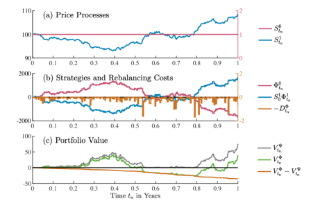
For the discretized Shiryaev strategy and our basis setting of Table 3.1, this figure plots a typical simulation result. Panel (a) shows the realized prices $S^{0}_{t_{n}}$ and $S^{1}_{t_{n}}$ of the risk-free and the risky asset, respectively. Panel (b) illustrates the strategy holdings $\Phi^{0}_{t_{n}}$ and $\Phi^{1}_{t_{n}}$ for these assets where the latter has been multiplied by $S_{0}^{1}$. Furthermore, it contains the negative rebalancing costs $-D_{t_{n}}^{\Phi}$. Finally, Panel (c) reports the portfolio value $V_{t_{n}}^{\Phi}$ of the strategy. It is supplemented by the value process $V_{t_{n}}^{\Psi}$ of continuous-time trading and the difference between both portfolio values which, except for terminal time $t_{N}=T=1$, is equal to the holdings $\Phi^{2}_{t_{n}}$ in the transaction account.

Figure 3.1: Exemplary realization of the discretized Shiryaev strategy

3.2.2 Impact of transaction costs

After examining a single simulation scenario in the parameter basis setting, we now turn to the results of 100,000 scenarios and additionally introduce transaction costs.

Panel (a) of Figure 3.2 visualizes the simulated distribution of the terminal portfolio value $V_{T}^{\Psi}$ for continuous-time trading and the corresponding $V_{T}^{\Phi}$ distributions for the discrete-time case with three different transaction cost variants. $p=(0,0)$ resembles no transaction costs. $p=(0.1,0)$ considers only proportional costs, whereas $p=(0.1,0.5)$ additionally includes a minimum fee. Recall that the proportional values are expressed in percent. The chosen cost magnitudes are guided by what are currently very low commissions and brokerage fees (see Auer and Schuhmacher, 2015). Table 3.2 provides summary statistics for the distributions and concisely evaluates the performance of the trading strategy. Here, we are particularly interested in the mean terminal value and the loss probability because they capture $\mathbb{E}(V_{T}^{\Phi})$ and $\mathbb{P}(V_{T}^{\Phi}<0)$, respectively.

We observe that the Shiryaev strategy $\Psi$ is an arbitrage strategy with positive terminal values $V_{T}^{\Psi}$ in all scenarios. In contrast, discretizing the strategy yields a terminal value $V_{T}^{\Phi}$ distribution of similar shape but shifted towards smaller values and partially into negative territory. Without transaction costs, the range of observed terminal values is $[-42.46,428.24]$. This means that the maximum gain is roughly ten times higher than the maximum loss. With a value of $112.93$, the mean of $V_{T}^{\Phi}$ is more than double the maximum loss. The former also covers about 75% of the mean of $V_{T}^{\Psi}$ which amounts to $148.26$. To earn such outcomes, the investor has to accept a loss probability of only 28%.

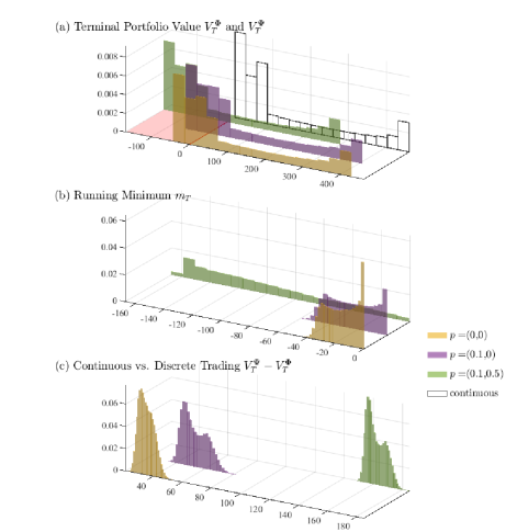
For $100,000$ scenarios of the discretized Shiryaev strategy, the basis setting of Table 3.1 and a range of transaction cost values, this figure presents various portfolio value distributions. Panel (a) shows the distributions of the terminal value $V_{T}^{\Phi}$ of discrete-time trading with alternative transaction costs $p=(p_{1},p_{2})$ where $p_{1}$ reflects proportional costs (in percent) and $p_{2}$ is a minimum fee (in monetary units). The loss region with negative terminal values is highlighted by a red floor. The distribution of the terminal value $V_{T}^{\Psi}$ of continuous-time trading is also included. Panel (b) contains the distributions of the running minimum $m_{T}$ of the discrete value processes, i.e., the worst-case portfolio values in the investment horizon. Finally, the distributions in Panel (c) refer to the terminal difference $V_{T}^{\Psi}-V_{T}^{\Phi}$ between continuous-time and discrete-time trading.

Figure 3.2: Shiryaev portfolio value distributions for different transaction costs

Strat.	Transact.	Mean	Stand.		Quantiles				Loss
	costs $p$		dev.	Min	5%	Median	95%	Max	prob.
$\Psi$	none	$148.26$	$155.10$	$7.5\times 10^{-8}$	$1.11$	$75.00$	$452.24$	$461.21$	$0$
$\Phi$	$(0,0)$	$112.93$	$151.44$	$-42.46$	$-31.42$	$43.59$	$409.99$	$428.24$	$0.28$
	$(0.1,0)$	$95.27$	$148.37$	$-59.41$	$-46.25$	$28.15$	$386.49$	$407.22$	$0.36$
	$(0.1,0.5)$	$-13.86$	$149.85$	$-167.46$	$-156.42$	$-82.54$	$280.32$	$298.66$	$0.67$

This table reports some descriptive statistics for the terminal portfolio value distributions in Panel (a) of Figure 3.2. Besides the mean and standard deviation, we compute the minima and maxima as well as selected quantiles. Furthermore, we present the simulated loss probability, i.e., the proportion of negative terminal portfolio values.

Table 3.2: Shiryaev portfolio value statistics for different transaction costs

In line with intuition, transaction costs shift the portfolio value distribution even further such that losses become higher and more likely. For $p=(0.1,0)$, the mean of $V_{T}^{\Phi}$ falls to $95.27$ but remains positive. Simultaneously, the loss probability rises to $36\%$ but can still be considered reasonably low (see Hogan et al., 2004). In contrast, $p=(0.1,0.5)$ generates a negative mean of $-13.86$ and a loss probability of $67\%$. The reason for this drastic impact of the minimum fee is that our basis setting is of low monetary scale such that the daily trading volumes are small and the minimum fee applies frequently. For $N=250$ trades, this often results in a total fee of $250\times p_{2}=125$ offsetting gains and causing high losses. Overall, while proportional transaction costs only slightly reduce the performance of the discretized strategy, minimum fees can render it unattractive for small-scale investors. However, large-scale investors with a higher scaling factor $\gamma$ and thus higher trading volumes do not suffer from this kind of problem.

Panel (b) of Figure 3.2 conducts a worst-case analysis similar to drawdown calculations in active risk management (see Schuhmacher and Eling, 2011). For $t\in[0,T]$, we define the running minimum process associated with the discrete-time value process $V^{\Phi}$ as

$$m_{t}:=\min_{t_{n}\leq t}\,V_{t_{n}}^{\Phi}.$$ (3.1)

With $t=T$, we obtain $m_{T}$ representing the least favorable portfolio value in the investment horizon $[0,T]$. The simulated distributions of $m_{T}$ show that its upper bound is zero because, across our transaction cost variants, we have $V_{0}^{\Phi}\leq 0$. The smallest values of $m_{T}$ are close to the minima of the terminal values $V_{T}^{\Phi}$ in Panel (a). However, a frequency comparison reveals that the vast majority of worst-case events do not cluster at time $T$.

Finally, Panel (c) shows the simulated distributions of the difference $V_{T}^{\Psi}-V_{T}^{\Phi}$ between the terminal portfolio values of continuous-time trading and its discrete-time counterparts. Discrepancies obviously rise with $p$. More demanding transaction cost variants require higher capital infusions, i.e., a more intensive usage of the transaction account.

3.2.3 Impact of asset model parameters

To implement the Shiryaev strategy, investors have to select a suitable risky asset. To support this choice, we study the impact of the asset parameters $(\mu,\sigma,H)$ on the performance of the strategy. This primarily involves constructing figures and tables in the style of Figure 3.2 and Table 3.2. However, instead of $p$, we now vary $(\mu,\sigma,H)$.

Drift $\mu$

Figure 3.3 and Table 3.3 start by considering the alternative drift parameters $\mu\in\{0,\pm 0.1,\pm 0.2\}$. Assets with higher absolute mean returns $\mu$ shift and extend the distribution of $V_{T}^{\Phi}$ towards larger terminal values because they fuel the strategy with more extreme prices. This effect is stronger for positive than for negative $\mu$ because upward movements are unbounded, whereas downward movements have a floor at a price level of zero. For example, starting from $72.14$ for $\mu=0$, the mean terminal value is $213.04$ for $\mu=0.1$ but only $137.96$ for $\mu=-0.1$. In contrast, the loss probabilities are quite symmetric in $\mu$. From 26% for $\mu=0$, they rise to about $40\%$ for $|\mu|=0.1$ and decrease to about $5\%$ for $|\mu|=0.2$. A similar feature can be observed for the running minimum $m_{T}$. For $\mu=0$, its distribution is almost uniform. For rising $|\mu|$, peaks near zero become more pronounced and excursions of the portfolio value significantly below zero less likely. $V_{T}^{\Psi}-V_{T}^{\Phi}$ is not symmetric in $\mu$. Instead, the distribution support increases with $\mu$ towards larger values. Hence, a higher $\mu$ induces more rebalancing costs in discrete-time trading.

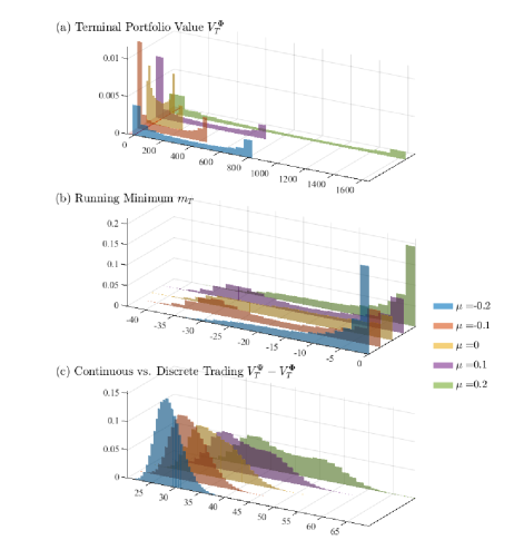
Similar to the Shiryaev strategy Figure 3.2, but for varying drift values $\mu$, this figure presents the simulated distributions of (a) the terminal portfolio value $V_{T}^{\Phi}$, (b) the running value process minimum $m_{T}$ and (c) the difference $V_{T}^{\Psi}-V_{T}^{\Phi}$ between the terminal portfolio values of continuous-time and discrete-time trading.

Figure 3.3: Shiryaev portfolio value distributions for different drifts

$\mu$	Mean	Median	Stand. dev.	Min	Max	Loss prob.
$-0.2$	356.05	302.32	297.61	$-11.85$	827.73	0.05
$-0.1$	137.96	61.73	174.54	$-42.05$	448.89	0.40
0	72.14	70.88	75.75	$-43.18$	211.32	0.26
0.1	213.40	71.86	272.22	$-43.30$	731.62	0.41
0.2	630.90	443.38	586.97	$-12.74$	1,648.65	0.05

Similar to Table 3.2, this table reports some descriptive statistics for the terminal portfolio value distributions in Panel (a) of Figure 3.3.

Table 3.3: Shiryaev portfolio value statistics for different drifts

Volatility $\sigma$

Figure 3.4 and Table 3.4 present our sensitivity results for the volatilities $\sigma\in\{0.05,0.10,0.15\}$. Increasing volatility goes along with a greater variability of terminal portfolio values $V_{T}^{\Phi}$. Large gains and large losses become more likely. This is also evident in the stretching distributions of the running minimum $m_{T}$. While the mean terminal values increase with $\sigma$, loss probabilities decrease. For example, $\sigma=0.05$ delivers $47.65$ and $41\%$, whereas $\sigma=0.15$ yields $223.71$ and 27%. Because investors receive more reward at lower risk, they have an incentive to opt for volatile assets (see Frazzini and Pedersen, 2014). However, there is a trade-off between these advantages and the rebalancing costs of discrete trading which are resembled by $V_{T}^{\Psi}-V_{T}^{\Phi}$ and substantially increase with $\sigma$.

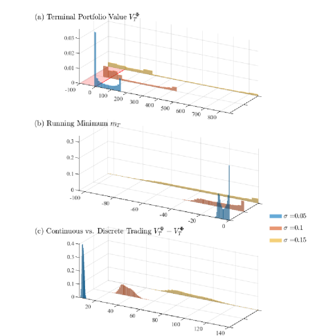
Similar to the Shiryaev strategy Figure 3.2, but for varying volatility values $\sigma$, this figure presents the simulated distributions of (a) the terminal portfolio value $V_{T}^{\Phi}$, (b) the running value process minimum $m_{T}$ and (c) the difference $V_{T}^{\Psi}-V_{T}^{\Phi}$ between the terminal portfolio values of continuous-time and discrete-time trading.

Figure 3.4: Shiryaev portfolio value distributions for different volatilities

$\sigma$	Mean	Median	Stand. dev.	Min	Max	Loss prob.
$0.05$	47.65	17.14	60.64	$-10.31$	161.11	0.41
$0.10$	112.94	43.59	151.44	$-42.45$	428.24	0.28
$0.15$	223.71	126.22	291.10	$-103.88$	857.36	0.27

Similar to Table 3.2, this table reports some descriptive statistics for the terminal portfolio value distributions in Panel (a) of Figure 3.4.

Table 3.4: Shiryaev portfolio value statistics for different volatilities

Hurst parameter $H$

In Figure 3.5 and Table 3.5, we investigate the Hurst coefficients $H\in\{0.51,0.55,0.60,0,65,0.70\}$. Recall that $H=0.5$ implies no memory and elevating $H$ within the interval $(0.5,1)$ establishes long memory. It generates positive serial correlation with levels linked to $H$ and high even for distant lags. Shiryaev-type investors take long (short) positions in the risky asset when its price deviates from an initial state in positive (negative) direction. Thus, they can benefit directly from a trending behavior of the risky asset which is more likely under high than low $H\in(0.5,1)$. Specifically, with rising $H$, the distributions of $V_{T}^{\Phi}$ and $m_{T}$ relocate such that the likelihood of large gains (losses) increases (decreases). Switching from $H=0.6$ to $H=0.7$, for example, raises the mean terminal value from $112.94$ to $138.39$ and lowers the loss probability from $28\%$ to $15\%$. Interestingly, this is accompanied by a sharp drop in rebalancing costs $V_{T}^{\Psi}-V_{T}^{\Phi}$. Hence, investors should trade assets with high $H$, which have been identified in many asset classes (see Hiemstra and Jones, 1997; Auer, 2016; Coakley et al., 2016), because they make the strategy more secure and less cash-intensive with respect to the transaction account.

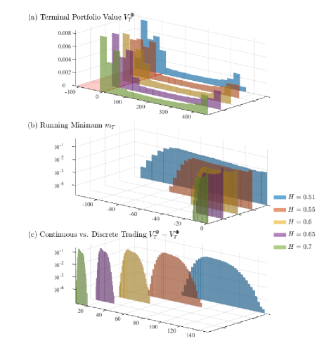
Similar to the Shiryaev strategy Figure 3.2, but for varying Hurst coefficients $H$, this figure presents the simulated distributions of (a) the terminal portfolio value $V_{T}^{\Phi}$, (b) the running value process minimum $m_{T}$ and (c) the difference $V_{T}^{\Psi}-V_{T}^{\Phi}$ between the terminal portfolio values of continuous-time and discrete-time trading. The vertical axes in Panels (b) and (c) are log-scaled.

Figure 3.5: Shiryaev portfolio value distributions for different Hurst coefficients

$H$	Mean	Median	Stand. dev.	Min	Max	Loss prob.
$0.51$	48.44	$-14.51$	142.18	$-118.00$	364.74	0.59
$0.55$	84.83	18.29	147.20	$-74.75$	399.25	0.40
$0.60$	112.94	43.60	151.44	$-42.46$	428.24	0.28
$0.65$	129.20	58.10	153.99	$-24.03$	445.74	0.21
$0.70$	138.39	66.27	155.31	$-13.76$	455.32	0.15

Similar to Table 3.2, this table reports some descriptive statistics for the terminal portfolio value distributions in Panel (a) of Figure 3.5.

Table 3.5: Shiryaev portfolio value statistics for different Hurst coefficients

3.2.4 Impact of trading horizon and frequency

Besides a suitable risky asset, Shiryaev-type investors have to decide on the trading horizon and frequency. Thus, it is instructive to know how they affect portfolio performance.

Trading horizon

In a first experiment, we fix the trading frequency to daily and vary the trading horizon $T$ between $6$ months and $10$ years. As far as the remaining parameters are concerned, we use the basis setting of Table 3.1 and the additional transaction cost settings of Figure 3.2 and Table 3.2. For each setting and trading horizon, we simulate 100,000 scenarios and report the mean terminal portfolio value and the loss probability in Figure 3.6. Panel (a) illustrates that the mean increases with the trading horizon and, except for the shortest horizons and the highest transaction costs, is positive-valued. Plugging (2.3) into (2.11), the terminal value of the continuous-time Shiryaev strategy is given by $V^{\Psi}_{T}=s_{0}^{1}\big{(}\exp\big{\{}\mu T+\sigma B_{T}^{H}\}-1\big{)}^{2}.$ Because $B_{T}^{H}$ is a centered Gaussian random variable with variance $T^{2H}$, we can deduce that, for large $T$, $\mathbb{E}(V^{\Psi}_{T})$ grows just like $s_{0}^{1}\exp\{2\mu T+2\sigma^{2}T^{2H}\}$. This exceeds exponential growth in $T$ because $H>0.5$. A similar behavior can be observed for the discretized strategy. Panel (b) shows that the loss probabilities initially decrease with $T$ and then stabilize at approximately $40\%$. The differences between our transaction cost variants shrink with $T$ and also stabilize. This can be explained by successively rising daily trading volumes eliminating the dominance of the minimum fee.

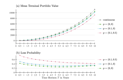
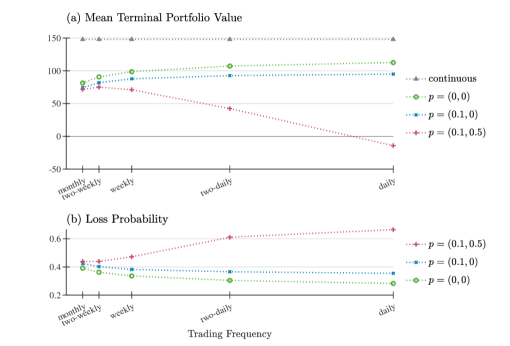
For 100,000 scenarios of the discretized Shiryaev strategy, the basis setting of Table 3.1 and a range of transaction cost values $p$, this figure plots (a) the mean of the terminal portfolio value and (b) the simulated loss probability against the trading horizon $T$. The continuous case is included as a reference.

Figure 3.6: Shiryaev sensitivity to trading horizon

Trading frequency

In a reverse second experiment, we fix the trading horizon to $T=1$ year and vary the trading frequency. We evaluate daily, two-daily, weekly, two-weekly and monthly rebalancing corresponding to 250, 125, 50, 25 and 12 trading periods per year. Figure 3.7 presents the simulation outcomes for our three transaction cost settings, i.e., the mean terminal value and the loss probability as functions of the trading frequency. The results for trading without transaction costs and only proportional costs are similar. The mean terminal value increases with the trading frequency but there is still a clear difference to continuous-time trading. The loss probability decreases with the trading frequency. For investors facing a supplementary minimum fee, the mean terminal value sharply drops with the trading frequency and reaches a negative value for daily trading. At the same time, the loss probability rises to more than $60\%$. This feature is again caused by the scale-related relative size of proportional costs and the minimum fee.

For 100,000 scenarios of the discretized Shiryaev strategy, the basis setting of Table 3.1 and a range of transaction cost values $p$, this figure plots (a) the mean of the terminal portfolio value and (b) the simulated loss probability against the trading frequency. The continuous case is included as a reference.

Figure 3.7: Shiryaev sensitivity to trading frequency

3.3 Discretized Salopek strategy

3.3.1 Impact of time discretization

We now turn to the Salopek strategy trading only risky assets and put special emphasis on a simple and practically appealing specification with $d=2$ assets. Following our approach for the Shiryaev strategy, Figure 3.8 starts by presenting a typical simulated realization in the basis setting of Table 3.1. This means that we plot the prices $S^{1}_{t_{n}}$ and $S^{2}_{t_{n}}$, the asset holdings $\Phi^{1}_{t_{n}}$ and $\Phi^{2}_{t_{n}}$, the negative rebalancing costs $-D_{t_{n}}^{\Phi}$ as well as the discrete and continuous strategy value processes $V_{t_{n}}^{\Phi}$ and $V_{t_{n}}^{\Psi}$ including their differences $V_{t_{n}}^{\Phi}-V_{t_{n}}^{\Psi}$.

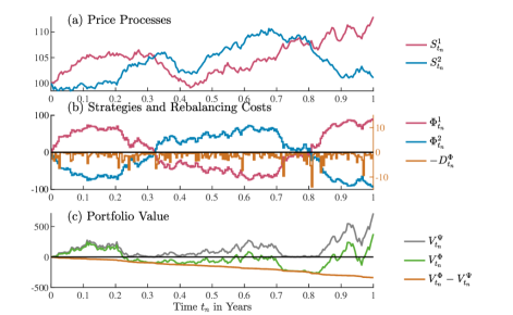
For the discretized Salopek strategy and our basis setting of Table 3.1, this figure plots a typical simulation result. Panel (a) shows the realized prices $S^{1}_{t_{n}}$ and $S^{2}_{t_{n}}$ of the two risky assets. Panel (b) illustrates the strategy holdings $\Phi^{1}_{t_{n}}$ and $\Phi^{2}_{t_{n}}$ for these assets. Furthermore, it contains the negative rebalancing costs $-D_{t_{n}}^{\Phi}$. Finally, Panel (c) reports the portfolio value $V_{t_{n}}^{\Phi}$ of the strategy. It is supplemented by the value process $V_{t_{n}}^{\Psi}$ of continuous-time trading and the difference between both portfolio values which, except for terminal time $t_{N}=T=1$, is equal to the holdings $\Phi^{3}_{t_{n}}$ in the transaction account.

Figure 3.8: Exemplary realization of the discretized Salopek strategy

In line with Proposition 2.1, we see that the investor is always long (short) in the asset with the higher (lower) price. Because the continuous-time value (2.16) tells us that $V_{t}^{\Psi}=M_{\beta}(S_{t})-M_{\alpha}(S_{t})\geq 0$, the properties of the $a$-order power mean $M_{a}(.)$ imply that the portfolio value of the Salopek strategy is all the greater the more the prices of the two assets deviate from each other. If they coincide, we have $M_{\beta}(S_{t})=M_{\alpha}(S_{t})$ and consequently a $V_{t}^{\Psi}$ of zero. These features are comparable to the Shiryaev strategy.

At first glance, it appears that there are also strong rebalancing cost similarities between the Shiryaev and Salopek strategies. For the Shiryaev strategy, we have shown that the rebalancing costs $D_{t_{n}}^{\Phi}$ are strictly positive for $n=1,\ldots,N-1$ (see Proposition 3.1). Figure 3.8 suggests the same property for the Salopek strategy. However, this does not hold in general. It can be verified via experiments with different choices of $(\alpha,\beta)$ that $D_{t_{n}}^{\Phi}$ may be negative for some $n$ (see, for example, Figure C.1 of the appendix). Thus, in contrast to the Shiryaev strategy, the portfolio value $V_{t_{n}}^{\Phi}$ of the discretized Salopek strategy can exceed the portfolio value $V_{t_{n}}^{\Psi}$ of its continuous-time counterpart.

3.3.2 Impact of transaction costs

Uniting all 100,000 simulation scenarios and charging transaction costs in the Salopek strategy, Figure 3.9 presents the distributions of the terminal portfolio values $V_{T}^{\Psi}$ and $V_{T}^{\Phi}$, the running minimum $m_{T}$ and the difference $V_{T}^{\Psi}-V_{T}^{\Phi}$. In addition, Table 3.6 reports summary statistics for the terminal value distributions.

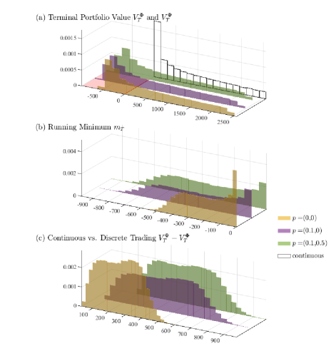
For $100,000$ scenarios of the discretized Salopek strategy, the basis setting of Table 3.1 and a range of transaction cost values, this figure presents various portfolio value distributions. Panel (a) shows the distributions of the terminal value $V_{T}^{\Phi}$ of discrete-time trading with alternative transaction costs $p=(p_{1},p_{2})$ where $p_{1}$ reflects proportional costs (in percent) and $p_{2}$ is a minimum fee (in monetary units). The loss region with negative terminal values is highlighted by a red floor. The distribution of the terminal value $V_{T}^{\Psi}$ of continuous-time trading is also included. Panel (b) contains the distributions of the running minimum $m_{T}$ of the discrete value processes, i.e., the worst-case portfolio values in the investment horizon. Finally, the distributions in Panel (c) refer to the terminal difference $V_{T}^{\Psi}-V_{T}^{\Phi}$ between continuous-time and discrete-time trading.

Figure 3.9: Salopek portfolio value distributions for different transaction costs

Strat.	Transact.	Mean	Stand.		Quantiles				Loss
	costs $p$		dev.	Min	5%	Median	95%	Max	prob.
$\Psi$	none	$859.52$	784.15	$1.25\times 10^{-9}$	2.54	643.28	2,327.94	2,559.70	$0$
$\Phi$	$(0,0)$	$592.14$	866.38	$-617.68$	$-403.23$	370.23	2,185.35	2,518.66	$0.36$
	$(0.1,0)$	$410.94$	916.00	$-959.37$	$-670.03$	185.63	2,078.98	2,472.87	$0.44$
	$(0.1,0.5)$	$362.70$	895.17	$-973.07$	$-690.48$	141.99	1,997.30	2,362.16	$0.46$

This table reports some descriptive statistics for the terminal portfolio value distributions in Panel (a) of Figure 3.9. Besides the mean and standard deviation, we compute the minima and maxima as well as selected quantiles. Furthermore, we present the simulated loss probability, i.e., the proportion of negative terminal portfolio values.

Table 3.6: Salopek portfolio value statistics for different transaction costs

Similar to the Shiryaev case, discretization and transaction costs expand the negative distribution support of $V_{T}^{\Phi}$ and $m_{T}$ and increase $V_{T}^{\Psi}-V_{T}^{\Phi}$. However, the Salopek strategy differs in notable aspects. First, without transaction costs, the means of $V_{T}^{\Phi}$ and $V_{T}^{\Psi}$ are $592.14$ and $859.52$, respectively. Because the former covers just about 69% of the latter, the Salopek strategy exhibits larger discretization shrinkage than the Shiryaev strategy. Second, turning to $p=(0.1,0)$, the terminal mean and loss probability are $410.94$ and $44\%$, respectively. These values are higher than for the Shiryaev strategy but must be put into the perspective that the Salopek strategy drains the transaction account more significantly than the Shiryaev strategy. Finally, for $p=(0.1,0.5)$, we observe a terminal mean of $362.70$ accompanied by a loss probability of $46\%$. While, in the Shiryaev case, the minimum fee causes a negative mean and a very high loss probability, this does not occur for the Salopek strategy because of its larger trading volumes. Overall, transaction costs do not crucially diminish the performance of the discretized strategy.

3.3.3 Impact of Hurst parameters

Our basis setting assumes that the Hurst coefficients of the traded assets are identical, i.e., $H^{1}=H^{2}$. Because this is not a necessary requirement for strategy execution, we also investigate Hurst values of different magnitudes. Given the complexity of this exercise, Figure 3.10 presents its results, i.e., the characteristics of the terminal portfolio value distributions, in three-dimensional form. For $H^{1},H^{2}\in[0.51,0.99]$ with $H^{1}\leq H^{2}$, Panel (a) plots the minimum, mean and maximum of $V_{T}^{\Phi}$. Panels (b), (c) and (d) cover the mean of the running minimum $m_{T}$, the loss probability and the mean of $V_{T}^{\Psi}-V_{T}^{\Phi}$, respectively.

Higher persistence pushes terminal values, limits the risk of loss and reduces capital infusions. If both $H^{1}$ and $H^{2}$ approach their limit value one, the loss probability and the mean of the running minimum are drawn to zero. Put differently, even though discretization yields $V_{T}^{\Psi}-V_{T}^{\Phi}\neq 0$, the discretized Salopek strategy converges to an almost perfect arbitrage strategy. This can be explained by the limiting behavior of the fBm $B^{H}$ for $H\to 1$. In this situation, (2.2) implies for the covariance $\textrm{Cov}(B_{t}^{H},B_{s}^{H})\to ts$ such that $B_{t}^{H}$ and $B_{s}^{H}$ are perfectly positively correlated for all $t,s>0$ and it can be deduced that $B_{t}^{H}=tB_{1}^{H}$. Because the fBm is a centered Gaussian process, we obtain $B^{H^{i}}_{t}=Z^{i}t$ with independent standard Gaussian random variables $Z^{i},i=1,2$. In this case, (2.3) delivers asset prices $S_{t}^{i}=s_{0}^{i}\exp\{\mu^{i}t+\sigma^{i}Z^{i}t\}$. Because their paths are exponential functions with growth rate $\mu^{i}+\sigma^{i}Z^{i}$, the quantities $Z^{i}$ are the only source of uncertainty. However, they are unveiled to the investor with the asset price observations at the first trading time $t_{1}$. This means that, after $t_{1}$, future asset prices are completely known. If the growth rate of $S^{1}$ is above (below) the one of $S^{2}$, we have $S^{1}_{t}>S^{2}_{t}$ ($S^{1}_{t}<S^{2}_{t}$) for all $t\in[0,T]$. Thus, a long position in the asset with the larger price and a short position in the other is a straightforward risk-free strategy.

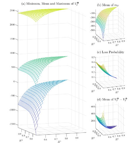
For $100,000$ scenarios of the discretized Salopek strategy, the basis setting of Table 3.1 and a range of Hurst parameter values $H^{1},H^{2}\in[0.51,0.99]$ with $H^{1}\leq H^{2}$, this figure characterizes the corresponding distributions of the terminal portfolio value $V_{T}^{\Phi}$. Panel (a) shows the minimum, mean and maximum of $V_{T}^{\Phi}$. Panel (b) plots the mean of the running minimum $m_{T}$. Panels (c) and (d) cover the simulated loss probability and the mean of the difference $V_{T}^{\Psi}-V_{T}^{\Phi}$ between continuous and discrete trading, respectively.

Figure 3.10: Salopek sensitivity to Hurst coefficients

3.3.4 Impact of strategy parameters

While Shiryaev-type investors have access to a unique trading rule, Salopek investors are confronted with a family of rules parameterized by $(\alpha,\beta)$. Consequently, they need to choose a suitable tuple $(\alpha,\beta)$ in practical applications. In the continuous-time case, (2.16) and (2.14) imply that the maximum portfolio value $V_{t}^{\Psi,\max}=\max\left(S_{t}^{1},S_{t}^{2}\right)-\min\left(S_{t}^{1},S_{t}^{2}\right)$ is attained for the limiting tuple $(\alpha,\beta)=(-\infty,\infty)$. With this setup, the strategy representation (2.12) tells us that $\Psi$ is a buy-and-hold strategy with a long position in the high-priced asset financed by short selling the low-priced asset as long as the sign of $S^{1}-S^{2}$ is unchanged. If a change occurs, i.e., if the price paths cross, the asset roles simply reverse.

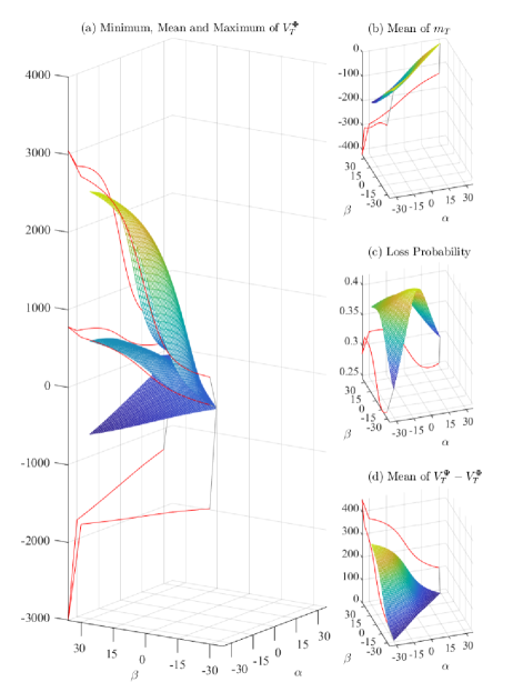
For $100,000$ scenarios of the discretized Salopek strategy, the basis setting of Table 3.1 and a range of strategy parameter values $\alpha\in[-30,29]$ and $\beta\in[\alpha+1,30]$, this figure characterizes the corresponding distributions of the terminal portfolio value $V_{T}^{\Phi}$. Panel (a) shows the minimum, mean and maximum of $V_{T}^{\Phi}$. Panel (b) plots the mean of the running minimum $m_{T}$. Panels (c) and (d) cover the simulated loss probability and the mean of the difference $V_{T}^{\Psi}-V_{T}^{\Phi}$ between continuous and discrete trading, respectively. The red lines represent the results for the limiting cases $\alpha=-\infty$ and $\beta=\infty$.

Figure 3.11: Salopek sensitivity to strategy parameters

Although the infinite setup is appealing from a theoretical point of view, the question arises whether it also maxes out in a discrete environment. Rebalancing costs may vary with $(\alpha,\beta)$ and suggest a different optimal parameter choice. To provide an answer, Figure 3.11 plots our set of previously used portfolio value characteristics against the parameters $\alpha\in[-30,29]$ and $\beta\in[\alpha+1,30]$. For $\alpha=\beta$, the Salopek positions and portfolio value are zero because we are not invested in any risky asset. With growing difference $\beta-\alpha$, the means of $V_{T}^{\Phi}$ and $V_{T}^{\Psi}-V_{T}^{\Phi}$ increase. They reach their maxima for the limit $\beta=-\alpha=\infty$. Thus, even though the rebalancing costs are also at their maximum, continuous-time and discrete-time trading both max in the same limiting case. With respect to the loss probabilities, we observe values between $24\%$ and $42\%$. For $\beta=-\alpha=\infty$, we have $28\%$. The highest probability arises for the tuple $(\alpha,\beta)=(0,1)$.

3.3.5 Impact of trading horizon and frequency

To complete our analysis of the Salopek strategy, we study its sensitivity to different trading horizons and frequencies and compare the findings to the Shiryaev strategy.

Trading horizon

Again, we start by enlarging the trading horizon $T$ and upholding a daily trading frequency. For our three transaction cost variants, Figure 3.12 displays the mean terminal portfolio value and the loss probability as functions of $T$. For both $\Psi$ and $\Phi$, Panel (a) suggests that the growth of the mean terminal values in the first ten years is only slightly faster than linear. This is in contrast to the Shiryaev strategy where we detected faster than exponential growth. While, for $T\leq 5.5$, the means of the Salopek strategy are larger than those of the Shiryaev strategy, the latter surpass the former for higher $T$. In particular, for $T=10$, the Shiryaev values exceed the Salopek values nearly twofold. In our drifting environment, this can be linked to the fact that the Shiryaev asset tends to deviate further from its initial price than the Salopek assets deviate from each other. Panel (b) shows that the loss probabilities decrease with $T$ and converge to a level of about $20\%$ ($30\%$, $35\%$) without (with) transaction costs. Hence, their magnitudes are smaller than for the Shiryaev strategy. Moreover, for increasing $T$, the loss probabilities related to transaction costs with a minimum fee do not approach those of purely proportional costs.

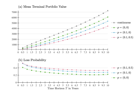
For 100,000 scenarios of the discretized Salopek strategy, the basis setting of Table 3.1 and a range of transaction cost values $p$, this figure plots (a) the mean of the terminal portfolio value and (b) the simulated loss probability against the trading horizon $T$. The continuous case is included as a reference.

Figure 3.12: Salopek sensitivity to trading horizon

Trading frequency

In a last simulation, Figure 3.13 sets diverse trading frequencies within a locked trading horizon of $T=1$ year. The resulting mean terminal portfolio values in Panel (a) imply that, even in the presence of transaction costs, higher trading frequencies are beneficial for investors. In contrast to the Shiryaev strategy, the impact of minimum fees is almost negligible at high frequencies. The loss probabilities in Panel (b) also recommend more frequent trading. The value of about $40\%$ for daily trading illustrates once more that unavoidable rebalancing costs in discrete-time trading induce losses that prevent the strategy from reaching the zero probability limit of an infinite trading frequency.

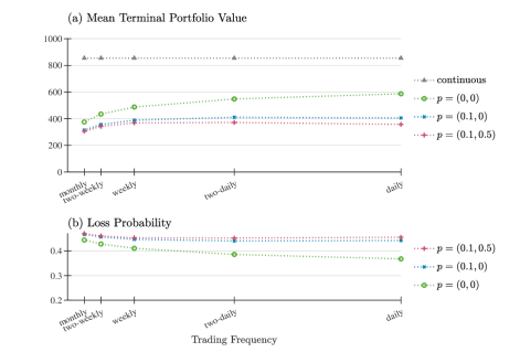
For 100,000 scenarios of the discretized Salopek strategy, the basis setting of Table 3.1 and a range of transaction cost values $p$, this figure plots (a) the mean of the terminal portfolio value and (b) the simulated loss probability against the trading frequency. The continuous case is included as a reference.

Figure 3.13: Salopek sensitivity to trading frequency

4 Conclusion

In this study, we have revisited the arbitrage strategies of Shiryaev (1998) and Salopek (1998) because they have a solid theoretical foundation and an elegant design making them highly appealing for investment practice. While the Shiryaev strategy trades only one risky asset and benefits from both rising and falling prices, the most elementary specification of the Salopek strategy trades two risky assets and capitalizes on prices drifting apart. Both strategies have very simple trading rules and rely only on realized prices, which are readily available in today’s investment world, so that they can be easily automated in modern algorithmic trading facilities.

Because these strategies aim at continuous-time trading in a fractional Black-Scholes market, we have transferred them to a discrete-time application and intensively studied their investment performance via Monte Carlo simulation. In conservative settings with independent assets, moderate serial correlation and realistic transaction costs, we show that, even though they can no longer be considered as arbitrage strategies, they exhibit positive terminal values on average and are accompanied by low loss probabilities. This makes them particularly interesting for tail-oriented investors (see Gao et al., 2018). Furthermore, we have revealed several interesting features of the discretized strategies. First, they perform reasonably well even if assets show relatively small persistence. Second, certain limiting cases of the strategies not only max out their performance but further simplify their implied asset positions. Third, time-discretization does not necessarily lead to portfolio values lower than in the continuous-time case. Finally, when adequately scaled, the strategies are useful for short-, medium- and long-term horizons and most advisable at a daily trading frequency. This nicely integrates into the growing literature on the welfare consequences of speeding up transactions in financial markets (see Du and Zhu, 2017).

Our study offers plenty of scope for future research. With respect to theoretical work, it is instructive to introduce an interest-bearing transaction account (with potentially differing rates for borrowing and lending). Furthermore, modeling a negative cross-correlation between risky assets can be considered a fruitful endeavor because it has the potential to increase strategy performance. It also makes the strategies comparable to the domain of pairs trading rules for correlated assets (see Krauss, 2017; Chen et al., 2017). As far as empirical work is concerned, we suggest a profound analysis of the Shiryaev and Salopek strategies in different asset classes. Such an analysis is complicated by the fact that traditional estimators of the Hurst coefficient (such as rescaled range and detrended fluctuation analysis) are highly sensitive to short time-series, short-term memory and non-normality. However, recent research has brought forth a variety of very promising estimators (see, for example, López-Garíca et al., 2021) which can serve as the basis for suitably capturing long memory and implementing investment strategies exploiting its dynamics.

Appendix

Appendix A Proofs of propositions

Proof (Proposition 2.1)

Recall the Salopek strategy (2.12) with $\Psi_{t}^{i}(\alpha,\beta)=\widehat{\Psi}_{t}^{i}(\beta)-\widehat{\Psi}_{t}^{i}(\alpha)$, where $\widehat{\Psi}_{t}^{i}(a)=\frac{1}{d}\left(\frac{S_{t}^{i}}{M_{a}(S_{t})}\right)^{a-1}$ and $M_{a}(x)$ is the (2.13) $a$-order power mean of $x=(x^{1},\ldots,x^{d})\in\mathbb{R}_{+}^{d}$.

We start with proving $\Psi_{t}^{i}(\alpha,\beta)>0$. Denoting $x={S_{t}^{i}}/{M_{\beta}(S_{t})}$ and $y={S_{t}^{i}}/{M_{\alpha}(S_{t})}$, relation (2.17) implies $1<x<y$ and $\beta\geq 1>\alpha$ gives $x^{\beta-1}\geq 1>y^{\alpha-1}$. Hence, $({S_{t}^{i}}/{M_{\beta}(S_{t})})^{\beta-1}>({S_{t}^{i}}/{M_{\alpha}(S_{t})})^{\alpha-1}$. This proves $\widehat{\Psi}_{t}^{i}(\beta)>\widehat{\Psi}_{t}^{i}(\alpha)$ from which the claim follows.

The proof of $\Psi_{t}^{j}(\alpha,\beta)<0$ is similar. Denoting $x={S_{t}^{j}}/{M_{\beta}(S_{t})}$ and $y={S_{t}^{j}}/{M_{\alpha}(S_{t})}$, relation (2.17) implies $0<x<y<1$ and $\beta\geq 1>\alpha$ gives $x^{\beta-1}\leq 1<y^{\alpha-1}$. Hence, $({S_{t}^{j}}/{M_{\beta}(S_{t})})^{\beta-1}<({S_{t}^{j}}/{M_{\alpha}(S_{t})})^{\alpha-1}$. This proves $\widehat{\Psi}_{t}^{j}(\beta)<\widehat{\Psi}_{t}^{j}(\alpha)$ from which the claim follows.

For the special case $S^{i}_{t}=S_{t}^{max}=\max\{S_{t}^{1},\ldots S_{t}^{d}\}$ and $S^{j}_{t}=S_{t}^{min}=\min\{S_{t}^{1},\ldots S_{t}^{d}\}$, the monotonicity property (2.14) of the $a$-order power mean $M_{a}(S_{t})$ saying that $S_{t}^{min}\leq M_{\alpha}(S_{t})\leq M_{\beta}(S_{t})\leq S_{t}^{max}$ implies (2.17). This completes the proof.

Proof (Proposition 3.1)

Substituting the Shiryaev strategy (2.10) into (2.26) and using $\Phi_{n}^{i}=\Psi_{t_{n-1}}^{i},n=1,\ldots,N,$ we have almost surely

$$D_{t_{n}}^{\Phi} =\frac{(S_{t_{n-1}}^{1})^{2}-(S_{t_{n}}^{1})^{2}}{s_{0}^{1}}S^{0}_{t_{n}}+\frac{2}{s_{0}^{1}}\big{(}S_{t_{n}}^{1}-S_{t_{n-1}}^{1}\big{)}S^{1}_{t_{n}}$$ (A.1)

$$=\frac{1}{s_{0}^{1}}\big{(}(S_{t_{n}}^{1})^{2}+(S_{t_{n-1}}^{1})^{2}-2S_{t_{n}}^{1}S_{t_{n-1}}^{1}\big{)}=\frac{(S_{t_{n}}^{1}-S_{t_{n-1}}^{1})^{2}}{s_{0}^{1}}>0.$$ (A.2)

Appendix B Spectral simulation

Various algorithms (such as midpoint displacement, Fourier filtering and spectral generation) have been proposed to simulate discrete-time fBms. Kijima and Tam (2013) give an overview of available (accurate and approximate) methods and conclude that, in the case of a finite time horizon, spectral techniques should be preferred. Therefore, we use the spectral method of Yin (1996). It is characterized by an efficient computation time and fully preserves the properties of a fBm.

The spectral method exploits the stationarity of fBm increments and is based on features of the discrete Fourier transformation and the central limit theorem. It relies on the theory of stationary discrete-time stochastic processes as well as the associated correlation and spectral theory. Here, it is convenient to consider two-sided processes $X=(X_{m})_{m\in\mathbb{Z}}$, where the index $m$ takes values in the set $\mathbb{Z}$ of all integers instead of just $\mathbb{N}_{0}=\{0,1,\ldots\}$. Stationary processes are typified by the correlation function $R_{X}(m)=\textrm{Cov}(X_{0},X_{m}),m\in\mathbb{Z}$, and the corresponding power spectral density

$$S_{X}(f) =\sum_{m=-\infty}^{\infty}R_{X}(m)\cos(2\pi mf)\quad\text{for}\quad-\frac{1}{2}\leq f\leq\frac{1}{2},$$ (B.1)

where $f$ is the frequency. $R_{X}$ and $S_{X}$ form a pair of discrete Fourier transforms.

Simulating a path of a fBm $B^{H}$ on $[0,T]$ involves generating realizations of $B^{H}$ at discrete times $t_{n}=n\Delta$, $n=0,\ldots,N$, with constant step size $\Delta=T/N$ for some $N\in\mathbb{N}$. It starts by producing $N$ increments of a fBm $\overline{B}^{H}$ on $[0,N]$ with unit step size $\Delta=1$, i.e., $W_{k}^{H}=\overline{B}_{k+1}^{H}-\overline{B}_{k}^{H}$, $k=0,\ldots,N-1$. Increment accumulation and self-similarity rescaling, i.e., $B_{t_{n+1}}^{H}=\left(\frac{T}{N}\right)^{H}\sum_{k=0}^{n}W_{k}^{H},n=0,\ldots,N-1,$ then approximate the discrete-time fBm $B^{H}$ on $[0,T]$.

According to Yin (1996), for $k=0,\ldots,N-1$, the increments $W_{k}^{H}$ can be proxied by

$$W_{k}^{H}=\sqrt{2N^{-1}}\sum_{j=-\frac{N}{2}}^{\frac{N}{2}-1}\left[S_{W}^{N}(jN^{-1})\right]^{\frac{1}{2}}\left[\cos(2\pi jkN^{-1})\cos(\varphi_{j})-\sin(2\pi jkN^{-1})\sin(\varphi_{j})\right].$$ (B.2)

Here, $S_{W}^{N}$ denotes the finite horizon approximation (B.3) of the power spectral density $S_{W}$ of the sequence of increments $(W_{k}^{H})$. $(\varphi_{j})$ is a sequence of independent random variables uniformly distributed on the interval $(0,2\pi)$.

For the increment process $W^{H}$ and the Hurst parameter $H>0.5$, the $S_{W}$ in (B.1) is not well-defined because of the long-range dependence of the fBm. This property implies that the correlation function of $W^{H}$, given by $R_{W}(m)=\frac{1}{2}(|m+1|^{2H}+|m-1|^{2H}-2|m|^{2H})$, does not decay fast enough for $|m|\to\infty$ and thus prevents the convergence of the infinite series in (B.1). Because we only need paths of the fBm $\overline{B}^{H}$ on the finite interval $[0,N]$ and ’very long memory’ effects cannot be observed on finite intervals, this problem can be circumvented by neglecting correlations for time lags larger than $N/2$. This means that, in (B.2), we do not use $S_{W}$ but

$$S_{W}^{N}(f)=\sum_{m=-\frac{N}{2}}^{\frac{N}{2}-1}\frac{1}{2}(|m+1|^{2H}+|m-1|^{2H}-2|m|^{2H})\cos(2\pi mf).$$ (B.3)

Computer implementations of the spectral method benefit from fast Fourier transformation (FFT) which improves computation time. As emphasized by Yin (1996), the increments $W_{k}^{H}$ in (B.2) can be obtained as the real part of a complex FFT where real and imaginary are $(S_{W}^{N}(jN^{-1}))^{\frac{1}{2}}\cos(\varphi_{j})$ and $(S_{W}^{N}(jN^{-1}))^{\frac{1}{2}}\sin(\varphi_{j})$, respectively.

Appendix C Additional figures

Figures C.1 and C.2 supply additional simulated realizations of the Salopek strategy to illustrate the effects of negative rebalancing costs and infinite strategy parameter values, respectively.

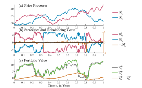
Using the overall design and setting of Figure 3.8, this figure simulates another exemplary realization of the Salopek strategy but replaces the $(\alpha,\beta)$ basis values of $(-30,30)$ by $(71,80)$.

Figure C.1: Realization of the discretized Salopek strategy with negative rebalancing costs

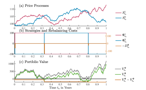
Using the overall design and setting of Figure 3.8, this figure simulates another exemplary realization of the Salopek strategy but replaces the $(\alpha,\beta)$ basis values of $(-30,30)$ by $(-\infty,\infty)$.

Figure C.2: Realization of the discretized Salopek strategy with parameter infinity

References

- Amblard et al. (2013) Amblard, P.O., Coeurjolly, J.F., Lavancier, F., Philippe, A., 2013. Basic properties of the multivariate fractional Brownian motion. Séminaires & Congrès 28, 65–87.
- Auer (2016) Auer, B.R., 2016. Pure return persistence, Hurst exponents, and hedge fund selection: a practical note. Journal of Asset Management 17, 319–330.
- Auer and Schuhmacher (2015) Auer, B.R., Schuhmacher, F., 2015. Liquid betting against beta in Dow Jones Industrial Average stocks. Financial Analysts Journal 71, 30–43.
- Badrinath and Gubellini (2011) Badrinath, S.G., Gubellini, S., 2011. On the characteristics and performance of long-short, market-neutral and bear mutual funds. Journal of Banking and Finance 35, 1762–1776.
- Barroso and Santa-Clara (2015) Barroso, P., Santa-Clara, P., 2015. Momentum has its moments. Journal of Financial Economics 116, 111–120.
- Bayraktar and Poor (2005) Bayraktar, E., Poor, H.V., 2005. Arbitrage in fractal modulated Black-Scholes models when the volatility is stochastic. International Journal of Theoretical and Applied Finance 8, 283–300.
- Bender et al. (2011) Bender, C., Sottinen, T., Valkeila, E., 2011. Fractional processes as models in stochastic finance, in: Nunno, G.D., Øksendal, B. (Eds.), Advanced Mathematical Methods for Finance, Springer, Berlin, Heidelberg. pp. 75–103.
- Bessembinder (2018) Bessembinder, H., 2018. Do stocks outperform Treasury bills? Journal of Financial Economics 129, 440–457.
- Biagini et al. (2008) Biagini, F., Hu, Y., Øksendal, B., Zhang, T., 2008. Stochastic Calculus for Fractional Brownian Motion and Applications. Springer, London.
- Björk (2004) Björk, T., 2004. Arbitrage Theory in Continuous Time. Oxford University Press, Oxford.
- Black and Scholes (1973) Black, F., Scholes, M., 1973. The pricing of options and corporate liabilities. Journal of Political Economy 81, 637–654.
- Bondarenko (2003) Bondarenko, O., 2003. Statistical arbitrage and securities prices. Review of Financial Studies 16, 875–919.
- Brock et al. (1992) Brock, W., Lakonishok, J., LeBaron, B., 1992. Simple technical trading rules and the stochastic properties of stock returns. Journal of Finance 47, 1731–1764.
- Chen et al. (2017) Chen, H.J., Chen, S.J., Chen, Z., Li, F., 2017. Empirical investigation of an equity pairs trading strategy. Management Science 65, 370–389.
- Cheridito (2003) Cheridito, P., 2003. Arbitrage in fractional Brownian motion models. Finance and Stochastics 7, 533–553.
- Chordia et al. (2014) Chordia, T., Subrahmanyam, A., Tong, Q., 2014. Have capital market anomalies attenuated in the recent era of high liquidity and trading activity? Journal of Accounting and Economics 58, 41–58.
- Coakley et al. (2016) Coakley, J., Kellard, N., Wang, J., 2016. Commodity futures returns: more memory than you might think! European Journal of Finance 22, 1457–1483.
- Cumova and Nawrocki (2014) Cumova, D., Nawrocki, D., 2014. Portfolio optimization in an upside potential and downside risk framework. Journal of Economics and Business 71, 68–89.
- Cutland et al. (1995) Cutland, N.J., Kopp, P.E., Willinger, W., 1995. Stock price returns and the Joseph effect: a fractional version of the Black-Scholes model, in: Bolthausen, E., Dozzi, M., Russo, F. (Eds.), Seminar on Stochastic Analysis, Random Fields and Applications, Springer, Berlin, Heidelberg. pp. 327–351.
- Delbaen and Schachermayer (1994) Delbaen, F., Schachermayer, W., 1994. A general version of the fundamental theorem of asset pricing. Mathematische Annalen 300, 463–520.
- Di Cesare et al. (2015) Di Cesare, A., Stork, P.A., De Vries, C.G., 2015. Risk measures for autocorrelated hedge fund returns. Journal of Financial Econometrics 13, 868–895.
- Du and Zhu (2017) Du, S., Zhu, H., 2017. What is the optimal trading frequency in financial markets? Review of Economic Studies 84, 1606–1651.
- Eling and Schuhmacher (2007) Eling, M., Schuhmacher, F., 2007. Does the choice of performance measure influence the evaluation of hedge funds? Journal of Banking and Finance 31, 2632–2647.
- Erb and Harvey (2006) Erb, C.B., Harvey, C.R., 2006. The strategic and tactical value of commodity futures. Financial Analysts Journal 62, 69–97.
- Frazzini and Pedersen (2014) Frazzini, A., Pedersen, L.H., 2014. Betting against beta. Journal of Financial Economics 111, 1–25.
- Gao et al. (2018) Gao, G.P., Lu, X., Song, Z., 2018. Tail risk concerns everywhere. Management Science 65, 3111–3130.
- Guasoni (2006) Guasoni, P., 2006. No arbitrage under transaction costs, with fractional Brownian motion and beyond. Mathematical Finance 16, 569–582.
- Guasoni et al. (2021) Guasoni, P., Mishura, Y., Rásonyi, M., 2021. High-frequency trading with fractional Brownian motion. Finance and Stochastics 25, 277–310.
- Guasoni et al. (2019) Guasoni, P., Nika, Z., Rásonyi, M., 2019. Trading fractional Brownian motion. SIAM Journal on Financial Mathematics 10, 769–789.
- Hardy et al. (1934) Hardy, G.H., Littlewood, J.E., Pólya, G., 1934. Inequalities. Cambridge University Press, Cambridge.
- Harrison et al. (1984) Harrison, J.M., Pitbladdo, R., Schaefer, S.M., 1984. Continuous price processes in frictionless markets have infinite variation. Journal of Business 57, 353–365.
- Hendricks and Singhal (2005) Hendricks, K.B., Singhal, V.R., 2005. An empirical analysis of the effect of supply chain disruptions on long-run stock price performance and equity risk of the firm. Production and Operations Management 14, 35–52.
- Hiemstra and Jones (1997) Hiemstra, C., Jones, J.D., 1997. Another look at long memory in common stock returns. Journal of Empirical Finance 4, 373–401.
- Hogan et al. (2004) Hogan, S., Jarrow, R., Teo, M., Warachka, M., 2004. Testing market efficiency using statistical arbitrage with applications to momentum and value strategies. Journal of Financial Economics 73, 525–565.
- Hong and Satchell (2015) Hong, K.J., Satchell, S., 2015. Time series momentum trading strategy and autocorrelation amplification. Quantitative Finance 15, 1471–1487.
- Hu and Øksendal (2003) Hu, Y., Øksendal, B., 2003. Fractional white noise calculus and applications to finance. Infinite Dimensional Analysis, Quantum Probability and Related Topics 6, 1–32.
- Jegadeesh and Titman (1993) Jegadeesh, N., Titman, S., 1993. Returns to buying winners and selling losers: implications for stock market efficiency. Journal of Finance 48, 65–91.
- Jegadeesh and Titman (2001) Jegadeesh, N., Titman, S., 2001. Profitability of momentum strategies: an evaluation of alternative explanations. Journal of Finance 56, 699–720.
- Kijima and Tam (2013) Kijima, M., Tam, C.M., 2013. Fractional Brownian motions in financial models and their Monte Carlo simulation, in: Chan, V.W.K. (Ed.), Theory and Applications of Monte Carlo Simulations. IntechOpen, Rijeka, pp. 53–85.
- Krauss (2017) Krauss, C., 2017. Statistical arbitrage pairs trading strategies: review and outlook. Journal of Economic Surveys 31, 513–545.
- López-Garíca et al. (2021) López-Garíca, M.N., Trinidad-Segovia, J.E., Sánchez-Granero, M.A., Pouchkarev, I., 2021. Extending the Fama and French model with a long term memory factor. European Journal of Operational Research 291, 421–426.
- Lütkebohmert and Sester (2019) Lütkebohmert, E., Sester, J., 2019. Robust statistical arbitrage strategies. Quantitative Finance 21, 379–402.
- Malceniece et al. (2019) Malceniece, L., Malcenieks, K., Putniņš, T.J., 2019. High frequency trading and comovement in financial markets. Journal of Financial Economics 134, 381–399.
- Mandelbrot and Ness (1968) Mandelbrot, B.B., Ness, J.W.V., 1968. Fractional Brownian motions, fractional noises and applications. SIAM Review 10, 422–437.
- Marshall et al. (2017) Marshall, B.R., Nguyen, N.H., Visaltanachoti, N., 2017. Time series momentum and moving average trading rules. Quantitative Finance 17, 405–421.
- Mishura (2008) Mishura, Y.S., 2008. Stochastic Calculus for Fractional Brownian Motion and Related Processes. Springer, Berlin, Heidelberg.
- Moskowitz et al. (2012) Moskowitz, T.Y., Ooi, Y.H., Pedersen, L.H., 2012. Time series momentum. Journal of Financial Economics 104, 228–250.
- Nascimento and Powell (2010) Nascimento, J., Powell, W., 2010. Dynamic programming models and algorithms for the mutual fund cash balance problem. Management Science 56, 801–815.
- Pan et al. (2004) Pan, M.S., Liano, K., Huang, G.C., 2004. Industry momentum strategies and autocorrelations in stock returns. Journal of Empirical Finance 11, 185–202.
- Rachev et al. (2007) Rachev, S., Jas̆ić, T., Stoyanov, S., Fabozzi, F.J., 2007. Momentum strategies based on reward-risk stock selection criteria. Journal of Banking and Finance 31, 2325–2346.
- Rogers (1997) Rogers, L.C.G., 1997. Arbitrage with fractional Brownian motion. Mathematical Finance 7, 95–105.
- Rostek and Schöbel (2013) Rostek, S., Schöbel, R., 2013. A note on the use of fractional Brownian motion for financial modeling. Economic Modelling 30, 30–35.
- Salopek (1998) Salopek, D.M., 1998. Tolerance to arbitrage. Stochastic Processes and their Applications 76, 217–230.
- Schuhmacher and Eling (2011) Schuhmacher, F., Eling, M., 2011. Sufficient conditions for expected utility to imply drawdown-based performance rankings. Journal of Banking and Finance 35, 2311–2318.
- Shiryaev (1998) Shiryaev, A.N., 1998. On arbitrage and replication for fractal models. MPS Working Paper No. 1998-20.
- Simutin (2014) Simutin, M., 2014. Cash holdings and mutual fund performance. Review of Finance 18, 1425–1464.
- Sottinen and Valkeila (2003) Sottinen, T., Valkeila, E., 2003. On arbitrage and replication in the fractional Black–Scholes pricing model. Statistics and Decisions 21, 93–107.
- Wang et al. (2012) Wang, X.T., Wu, M., Zhou, Z.M., Jing, W.S., 2012. Pricing European option with transaction costs under the fractional long memory stochastic volatility model. Physica A: Statistical Mechanics and its Applications 391, 1469–1480.
- Willinger et al. (1999) Willinger, W., Taqqu, M.S., Teverovsky, V., 1999. Stock market prices and long-range dependence. Finance and Stochastics 3, 1–13.
- Yin (1996) Yin, Z.M., 1996. New methods for simulation of fractional Brownian motion. Journal of Computional Physics 127, 66–72.