An efficient class of increasingly high-order ENO schemes with multi-resolution

Abstract

We construct an efficient class of increasingly high-order (up to 17th-order) essentially non-oscillatory schemes with multi-resolution (ENO-MR) for solving hyperbolic conservation laws. The candidate stencils for constructing ENO-MR schemes range from first-order one-point stencil increasingly up to the designed very high-order stencil. The proposed ENO-MR schemes adopt a very simple and efficient strategy that only requires the computation of the highest-order derivatives of a part of candidate stencils. Besides simplicity and high efficiency, ENO-MR schemes are completely parameter-free and essentially scale-invariant. Theoretical analysis and numerical computations show that ENO-MR schemes achieve designed high-order convergence in smooth regions which may contain high-order critical points (local extrema) and retain ENO property for strong shocks. In addition, ENO-MR schemes could capture complex flow structures very well.

Keywords high-order schemes  $\cdot$ ENO  $\cdot$ WENO  $\cdot$ finite difference scheme  $\cdot$ hyperbolic conservation laws

1 Introduction

Hyperbolic conservation laws are ubiquitous in nature. Although the corresponding partial differential equations (PDE) only involve first-order derivatives, their solutions are not easy because they usually contain both discontinuities and sophisticated structures with multi-scales. Therefore, high-order numerical schemes with excellent shock-capturing and multi-resolution properties are desired for solving hyperbolic conservation laws. The essentially non-oscillatory (ENO) schemes and weighted ENO (WENO) schemes are cutting-edge high-order shock-capturing schemes and achieve great success in practice.

Harten and his coworkers Harten et al. (1987) proposed the first ENO scheme which adaptively selects the smoothest stencil from several local candidates of the same size such that the constructed scheme achieves uniformly high order in smooth regions and suppresses non-physical oscillations near discontinuities. Shu and Osher Shu and Osher (1988, 1989) significantly improve the efficiency of ENO schemes by the method of lines. In their approach, the cell average reconstructions are replaced by numerical flux reconstructions which can be implemented in a dimension-by-dimension manner, and the time is discretized by an efficient Runge-Kutta scheme which preserves strong stability. The drawback of ENO schemes is that they only achieve the order of a small sub-stencil even when the whole global stencil is smooth. To improve ENO schemes, Liu et al. Liu et al. (1994) proposed a WENO scheme which combines all the candidate stencils via nonlinear weights. The weight becomes very tiny if the corresponding stencil contains discontinuities so that the constructed schemes achieve non-oscillatory features near discontinuities. However, these WENO schemes still cannot achieve the optimal order when the global stencils are smooth. Jiang and Shu Jiang and Shu (1996) systematically analyzed WENO schemes and provided a general framework for calculating smoothness indicators and nonlinear weights so that the constructed WENO schemes can retrieve the optimal order in smooth regions while retaining oscillatory at discontinuities. Henrick et al. Henrick et al. (2005) discovered that the WENO schemes proposed by Jiang and Shu lose accuracy at critical points (local extrema) if the parameter $\varepsilon$, which is used to avoid dividing by 0, is set to a very small number. They proposed a simple mapping function to modify the nonlinear to cure this issue. Borges et al. Borges et al. (2008) further improved the accuracy of WENO schemes by introducing a global smoothness and proposed the so-called WENO-Z type nonlinear weights. Yamaleev and Carpenter Yamaleev and Carpenter (2009a, b) proposed energy stable WENO (ESWENO) for systems of linear hyperbolic equations with both continuous and discontinuous solutions. The stability of $L_{2}$ norm is explicitly achieved (even when a purely downwind stencil is included) by enforcing a nonlinear summation-by-parts (SBP) condition at each instant in time. Hu et al. Hu et al. (2010) constructed an adaptive central-upwind scheme by adding an extra purely downwind stencil which is assigned with the smoothness indicator of the global central stencil. When the central stencil is nonsmooth, the effect of the purely downwind stencil is automatically excluded and the upwind shock-capturing WENO scheme is recovered. Fu et al. Fu et al. (2016, 2017, 2018); Fu (2021, 2023) proposed a family of targeted ENO (TENO) schemes which find out candidate stencils containing discontinuities and reconstruct an optimal flux based on the remaining stencil by using a scale separation strategy. In this way, TENO schemes significantly reduce numerical dissipation while maintaining ENO properties at discontinuities. Balsara and Shu Balsara and Shu (2000) found that very high-order extensions of WENO schemes may not always be monotonicity preserving. They constructed increasingly high-order (up to 11th-order) monotonicity preserving WENO by coupling the nonlinear weights of Jiang and Shu Jiang and Shu (1996) and the monotonicity preserving bounds of Suresh and Huynh Suresh and Huynh (1997). Gerolymos et al. Gerolymos et al. (2009) extended the mapped WENO scheme of Henrick et al. Henrick et al. (2005) to very-high-order (up to 17th-order) by coupling with a recursive-order-reduction (ROR) algorithm. Wu et al. Wu et al. (2021) improved the efficiency of the very-high-order WENO schemes by using efficient smoothness indicators Wu et al. (2020) and a predetermined order reduction method. Nowadays, there are many variants of ENO/WENO schemes and other shock-capturing high-order schemes adopting ENO/WENO idea, such as the weighted compact nonlinear schemes (WCNS) Deng and Zhang (2000), the central WENO (CWENO) schemes Bianco et al. (1999); Levy et al. (1999, 2000a), the hybrid compact-WENO schemes Pirozzoli (2002); Ren and Zhang (2003), the Hermite WENO (HWENO) schemes Qiu and Shu (2004, 2005), the WENO-ADER schemes Titarev and Toro (2002, 2004); Balsara et al. (2013), the $P_{N}P_{M}$ schemes Dumbser et al. (2008); Dumbser and Zanotti (2009); Dumbser (2010), and so forth. It is impossible to review all of them here. For more details on the development of ENO/WENO schemes, one may refer to the review by Shu Shu (2009, 2016).

The classical ENO/WENO schemes are constructed based on candidate stencils of an equal size which cannot achieve optimal accuracy in some cases. Taking five-point schemes for example, ENO schemes only choose the smoothest stencil among the three three-point candidate sub-stencils, and WENO schemes combine all three sub-stencils by nonlinear weights which may recover the optimal accuracy on the global stencil. However, in some cases, a non-smooth five-point global stencil may contain a smooth four-point sub-stencil, and in some other cases, all the three three-point sub-stencils may be non-smooth. Therefore, it is a natural choice to construct numerical schemes based on candidate stencils of unequal sizes. Levy et al. Levy et al. (2000b) first proposed a compact central WENO reconstruction which is a nonlinear combination of two two-point stencils and one three-point stencil. In smooth regions, the scheme approaches the three-point stencil, while near discontinuities, the scheme approaches the smoother two-point stencil for shock-capturing. The advantage of this approach is that it can recover the optimal high-order accuracy without constraint on the choice of linear weights like classical WENO schemes. In recent years, CWENO schemes based on the reconstruction technique by using stencils of unequal sizes have been substantially analyzed and developed by Puppo, Semplice, Dumbser, and Cravero et al. Puppo et al. (2022); Semplice et al. (2016, 2021); Semplice and Visconti (2020); Dumbser et al. (2017); Cravero and Semplice (2016); Cravero et al. (2018a, b). Cravero, Semplice, and Visconti Cravero et al. (2019) comprehensively reviewed such CWENO schemes. Inspired by the weighting strategy of Levy et al. Levy et al. (2000b), Zhu el al. Zhu and Qiu (2016); Zhu and Shu (2018, 2019, 2020) and Balsara et al. Balsara et al. (2016, 2020) constructed WENO schemes with adaptive order (WENO-AO) and multi-resolution (WENO-MR). Shen Shen (2021) proposed a simplified weighting strategy for combining polynomials of different degree and adopted it to construct weighted compact central schemes (WCCS) Shen et al. (2022). Fu et al. Fu et al. (2018) constructed high-order schemes with adaptive order based on candidate stencils of unequal sizes under the framework of TENO schemes. Shen Shen (2023) constructed a class of ENO schemes with adaptive order (ENO-AO) by using newly defined smoothness indicators which measure the minimum error between the reconstructed polynomial and the target function at the cells adjacent to corresponding stencils. The computation of the new smoothness indicator is simpler than that of Jiang and Shu’s smoothness indicator Jiang and Shu (1996), so ENO-AO schemes cost less CPU times than WENO-AO and TENO-AO schemes adopting Jiang and Shu’s smoothness indicator.

Multi-level ENO/WENO schemes constructed on candidate stencils of unequal sizes naturally have some advantages over those schemes constructed on candidate stencils of an equal size, so they have attracted a lot of attention and have undergone major development recently. However, there are still some challenges to be resolved. Firstly, the high-order accuracy is easily polluted by low-order candidate stencils, if special care is not exerted. Arbogast et al. Arbogast et al. (2018) proved that the highest order $r$ and the lowest order $s$ of multi-level reconstructions must satisfy $r\leq 2s-1$ when WENO-JS weights are used; and there is no constraint on $r$ and $s$ when WENO-Z weights are used, providing that enough intermediate levels or large enough power parameters in the weights are used. Secondly, when extended to very high-order situations, multi-level reconstruction may contain a lot of candidate stencils of different levels which significantly increases the complexity. We notice that existing multi-level ENO/WENO schemes rarely include low-order one-point and two-point candidate stencils. The existing high-order multi-level schemes, e.g., 9th-order WENO-AO(9,5,3) of Balsara et al. Balsara et al. (2016), 10th-order TENO10-AA scheme of Fu Fu (2021), and 9th-order multi-resolution WENO scheme of Zhu and Shu Zhu and Shu (2018), do not include candidate stencils of all levels. Zhu et al. Zhu and Qiu (2016); Zhu and Shu (2018, 2019, 2020) constructed WENO schemes by combining first- and second-order polynomials with high-order polynomials. To achieve optimal accuracy in smooth regions, the exponent of global smoothness indicators in the numerator must be larger than that appears in the denominator. As a result, the weights are not dimensionless, and the performance of the constructed schemes is problem-dependent Balsara et al. (2016). The ENO-AO schemes of Shen Shen (2023) consider one-point and two-point stencils as candidates, but they have a sensitive parameter $\varepsilon$ as well. When the smoothness indicator of a high-order stencil is smaller than $\varepsilon$, it will be considered to be a smooth stencil which guarantees optimal convergence order in smooth regions. Apparently, the choice of $\varepsilon$ may affect the convergence order. Some studies particularly discussed the effect of $\varepsilon$ Don and Borges (2013); Wang et al. (2019); Don et al. (2022). In addition, ENO-AO schemes select the smoothest stencil from all candidates. When extending to very high-order cases, the complexity of the selecting procedure will significantly increase.

In this study, we further simplify and improve the selecting strategy of ENO-AO schemes Shen (2023) and construct an efficient class of very-high-order ENO schemes with multi-resolution (ENO-MR) which have the following advantages:

• The candidates of ENO-MR schemes consist of all levels ranging from first-order up to the designed high-order (up to 17th-order).

• The selecting strategy only requires the computation of the highest-order derivatives of a part of candidate stencils which is beneficial to efficient implementation.

• ENO-MR schemes are endowed with an adaptive order-reduction mechanism, so very-high-order extensions do not require additional techniques to improve the robustness as very-high-order WENO schemes of Gerolymos et al. Gerolymos et al. (2009) and Wu et al. Wu et al. (2021) do.

• ENO-MR schemes are completely parameter-free and essentially scale-invariant.

• ENO-MR schemes achieve designed high-order convergence at high-order critical points (local extrema) without any additional treatment.

2 Finite difference ENO/WENO schemes

2.1 A semi-discretized conservative finite difference scheme

We consider the one-dimensional scalar conservation law,

$$\frac{\partial u}{\partial t}+\frac{\partial f(u)}{\partial x}=0,t\in[0,\infty),$$ (1)

in the spatial domain $[x_{L},x_{R}]$ that is discretized into uniform intervals by $x_{j}=x_{L}+(j-1)h$ ($j=1\text{ to }N+1$), where $h=(x_{R}-x_{L})/N$. Define a function $\mathcal{H}(x)$ implicitly as Shu and Osher (1988)

$$f(u(x))=\frac{1}{h}\int_{x-h/2}^{x+h/2}\mathcal{H}(\xi)d\xi.$$ (2)

Then we can get a semi-discretized conservative finite difference scheme as

$$\frac{du_{j}(t)}{dt}=\mathcal{L}(u_{j}(t))=-\frac{\hat{f}_{j+1/2}-\hat{f}_{j-1/2}}{h},$$ (3)

where the numerical flux $\hat{f}_{j\pm 1/2}$ is an approximation of the function $\mathcal{H}(x)$ at $x_{j\pm 1/2}$. The attractive feature of this approach is that it can be easily extended to multi-dimensional cases in a dimension-by-dimension manner.

To take account of the upwind mechanism which can improve the robustness of the scheme, we usually split the flux into two parts as

$$f(u)=f^{+}(u)+f^{-}(u),$$ (4)

where $\frac{df^{+}(u)}{du}\geq 0$ and $\frac{df^{-}(u)}{du}\leq 0$. Here, we adopt the global Lax–Friedrichs flux splitting method which is expressed as

$$f^{\pm}(u)=\frac{1}{2}(f(u)\pm\alpha u),$$ (5)

where $\alpha=\mbox{max}\left|\frac{df(u)}{du}\right|$ and the maximum is taken over all mesh points on one axis-aligned line.

2.2 Review of ENO/WENO flux reconstructions

2.2.1 Classical ENO/WENO reconstructions on candidate stencils of an equal size

Now, the remaining task is finding a proper way to calculate $\hat{f}_{j\pm 1/2}^{\pm}(u)$. To this end, we define a stencil $S_{j-m}^{j+n}$ as a set of successive intervals including $I_{j}$, i.e.,$S_{j-m}^{j+n}:=\{I_{j-m},...,I_{j},...,I_{j+n}\}$ ($m\geq 0,n\geq 0$). Then, we can trivially reconstruct a polynomial $P_{j-m}^{j+n}(x)$ of degree $m+n$ to approximate $\mathcal{H}(x)$ by enforcing the conservation conditions on $S_{j-m}^{j+n}$, i.e.,

$$\frac{1}{h}\int_{I_{k}}P_{j-m}^{j+n}(\xi)d\xi=f_{k},\quad k=j-m\text{ to }j+n.$$ (6)

Finally, the fluxes are simply calculate as $\hat{f}_{j\pm 1/2}=P_{j-m}^{j+n}\left(x_{j\pm 1/2}\right)$ which can be written in terms of $f_{k}$ as

$$\hat{f}_{j+1/2}=\sum_{l=-m}^{n}a_{l}f_{j+l}.$$ (7)

We note that we do not distinguish between $f^{+}$ and $f^{-}$ hereafter, because they are calculated by the same principle.

We have many choices for the stencil. When $f(u(x))$ is sufficiently smooth on $S_{j-m}^{j+n}$, $P_{j-m}^{j+n}$ is a $(m+n+1)$th-order approximation to $\mathcal{H}(x)$. Otherwise, $P_{j-m}^{j+n}$ is not a good approximation to $\mathcal{H}(x)$. When reconstructing fluxes, we should avoid stencils containing discontinuities. The $(2r-1)$-point ENO scheme Harten et al. (1987) selects the smoothest stencil from the pool of $r$-point candidate stencils $\{S_{j-r+1}^{j},S_{j-r+2}^{j+1},...,S_{j-1}^{j+r-2},S_{j}^{j+r-1}\}$, so it can only achieve at most $r$th-order accuracy. Classical WENO schemes use a weighted combination of the reconstructions on the same candidate stencils which can retrieve the $(2r-1)$-order reconstruction on the global stencil $S_{j-r+1}^{j+r-1}$ in smooth regions while retaining ENO properties at discontinuities. The formulae of standard $(2r-1)$-point WENO reconstructions are expressed as

$$P_{WENO}(x)=\sum_{k=0}^{r-1}\omega_{k}^{(r)}P_{j-r+k+1}^{j+k}(x),$$ (8a)

with

$$\omega_{k}^{(r)}=\frac{\alpha_{k}^{(r)}}{\sum_{l=0}^{r-1}\alpha_{l}^{(r)}},k=0,...,r-1.$$ (8b)

The nonlinear weights of Jiang and Shu Jiang and Shu (1996) are calculated as

$$\alpha_{k}^{(r,JS)}=\frac{d_{k}^{(r)}}{\left(\beta_{k}^{(r)}+\varepsilon\right)^{p}},k=0,...,r-1,$$ (9a)

with the smoothness indicators defined as

$$\beta_{k}^{(r)}=\sum_{l=1}^{r-1}h^{2l-1}\int_{x_{i-1/2}}^{x_{i+1/2}}\left(\frac{d^{l}P_{j-r+k+1}^{j+k}(x)}{dx^{l}}\right)^{2}dx,k=0,...,r-1.$$ (9b)

The WENO-Z type nonlinear weights Borges et al. (2008) are calculated as

$$\alpha_{k}^{(r,Z)}=d_{k}^{(r)}\left(1+\left(\frac{\tau_{2r-1}}{\beta_{k}^{(r)}+\varepsilon}\right)^{p}\right),k=0,...,r-1,$$ (10a)

with the global smoothness indicators defined as Castro et al. (2011)

$$\tau_{2r-1}=\begin{cases}\left|\beta_{0}^{(r)}-\beta_{r-1}^{(r)}\right|,\text{mod}(r,2)=1,\\ \\ \left|\beta_{0}^{(r)}-\beta_{1}^{(r)}-\beta_{r-2}^{(r)}+\beta_{r-1}^{(r)}\right|,\text{mod}(r,2)=0.\end{cases}$$ (10b)

We note that in both WENO-JS and WENO-Z weights, there are common parameters, namely $d_{k}^{(r)}$, $\varepsilon$, and $p$. $d_{k}^{(r)}$ are optimal linear weights which guarantee the optimal $(2r-1)$th-order in smooth regions. They may become negative or even non-existent in some cases. $\varepsilon$ is a tiny positive number used to avoid dividing by 0. The convergence rates of WENO schemes are found to be sensitive to $\varepsilon$ Don and Borges (2013). Gerolymos et al. Gerolymos et al. (2009) found that $p=2$ is sufficient to keep ENO property for $r\leq 6$ cases, but we have to use $p=r$ for $r>6$ cases. When solving Euler equations by very-high-order WENO schemes, the interaction between characteristic fields and/or the absence of a zone of smoothness of $r$ points to choose a stencil from may cause serious non-physical oscillations Harten et al. (1987). Order-reduction techniques are employed to retain ENO property Gerolymos et al. (2009); Wu et al. (2021).

2.2.2 ENO/WENO reconstructions on candidate stencils of unequal sizes

Levy et al. Levy et al. (2000b) first proposed a CWENO reconstruction based on two two-point stencils and one three-point stencil. In recent years, many WENO reconstructions with adaptive order (WENO-AO) with similar forms have been proposed based on this framework. Here, we briefly summarize the WENO-AO schemes proposed by Balsara et al. Balsara et al. (2016). The candidate stencils of WENO-AO($2r-1$,3) consist of $\{S_{j-r+1}^{j+r-1},S_{j-2}^{j},S_{j-1}^{j+1},S_{j}^{j+2}\}$ ($r\geq 3$). The final reconstructed polynomial is expressed as

$$P_{AO(2r-1,3)}(x) =\frac{\omega_{r-1}^{(2r-1)}}{d_{r-1}^{(2r-1)}}\left(P_{j-r+1}^{j+r-1}(x)-d_{0}^{(3)}P_{j-2}^{j}(x)-d_{1}^{(3)}P_{j-1}^{j+1}(x)-d_{2}^{(3)}P_{j}^{j+2}(x)\right)$$ (11)

$$+\omega_{0}^{(3)}P_{j-2}^{j}(x)+\omega_{1}^{(3)}P_{j-1}^{j+1}(x)+\omega_{2}^{(3)}P_{j}^{j+2}(x),$$

where $\omega$ can be calculated via WENO-JS weights or WENO-Z weights. The corresponding linear weights can be set as

$$d_{r-1}^{(2r-1)}=\gamma_{Hi},\quad d_{0}^{(3)}=d_{2}^{(3)}=(1-\gamma_{Hi})(1-\gamma_{Lo})/2,\quad d_{1}^{(3)}=(1-\gamma_{Hi})\gamma_{Lo},$$ (12)

where $\gamma_{Hi}\in[0.85,0.95]$ and $\gamma_{Lo}\in[0.85,0.95]$. Since the global $(2r-1)$-point stencil itself is a candidate stencil, WENO-AO reconstructions can recover the optimal $(2r-1)$th-order without particular constraints on the choice of linear weights. Furthermore, unlike WENO reconstructions based on candidate stencils of an equal size, the smallest candidate stencils of WENO-AO always contain three points regardless of the size of the global stencil. We can also include two-point stencils, for example Levy et al. (2000b); Zhu and Qiu (2016); Zhu and Shu (2018, 2019, 2020).

Combining several WENO-AO($2r-1$,3) reconstructions together, Balsara et al. Balsara et al. (2016) further proposed recursively defined WENO-AO reconstructions. For example, the WENO-AO(7,5,3) reconstruction can be expressed as

$$P_{AO(7,5,3)}(x)=\frac{\omega_{AO(7,3)}}{\gamma_{Hi}}\left(P_{AO(7,3)}(x)-(1-\gamma_{Hi})P_{AO(5,3)}(x)\right)+\omega_{AO(5,3)}P_{AO(5,3)},$$ (13a)

where,

$$\omega_{AO(7,3)}=\frac{\alpha_{AO(7,3)}}{\alpha_{AO(7,3)}+\alpha_{AO(5,3)}},\quad\omega_{AO(5,3)}=\frac{\alpha_{AO(5,3)}}{\alpha_{AO(7,3)}+\alpha_{AO(5,3)}}$$ (13b)

$$\alpha_{AO(7,3)}=\gamma_{Hi}\left(1+\frac{\sigma}{\beta_{3}^{(7)}+\varepsilon}\right),\alpha_{AO(5,3)}=(1-\gamma_{Hi})\left(1+\frac{\sigma}{\beta_{2}^{(5)}+\varepsilon}\right)$$ (13c)

with

$$\sigma=\left|\beta_{3}^{(7)}-\beta_{2}^{(5)}\right|.$$ (13d)

In theory, we can construct WENO-AO schemes by combining candidate stencils of arbitrary points. However, the nonlinear weights depend on the smoothness indicators defined by Eq. (9b) which is computationally expensive for high-order polynomials. Therefore, it is not practical to recursively construct very high-order WENO-AO schemes with many levels.

In order to improve the efficiency, Shen Shen (2023) proposed new smoothness indicators of $S_{j-m}^{j+n}$

$$IS_{j-m}^{j+n}={\rm MIN}(\delta_{L},\delta_{R}),$$ (14a)

where,

$$\delta_{L}=\begin{cases}\frac{1}{2}\left(\left|f_{j}-f_{j-1}\right|+\left|f_{j-1}-f_{j-2}\right|\right),\quad m=n=0,\\ \left|\frac{1}{h}\int_{I_{j-m-1}}P_{j-m}^{j+n}(\xi)d\xi-f_{j-m-1}\right|,\quad{\rm otherwise},\end{cases}$$ (14b)

$$\delta_{R}=\begin{cases}\frac{1}{2}\left(\left|f_{j}-f_{j+1}\right|+\left|f_{j+1}-f_{j+2}\right|\right),\quad m=n=0,\\ \left|\frac{1}{h}\int_{I_{j+n+1}}P_{j-m}^{j+n}(\xi)d\xi-f_{j+n+1}\right|,\quad{\rm otherwise}.\end{cases}$$ (14c)

The new smoothness indicators measure the minimum error between the reconstructed polynomial and the target function at the cells adjacent to $S_{j-m}^{j+n}$ which is not sensitive to the stencil size. Obviously, the new smoothness indicators are computationally cheaper than Jiang and Shu’s smoothness indicators which are defined by Eq. (9b). Utilizing the new smoothness indicators, a $(2r-1)$-point ENO-AO schemes are constructed in the following way:

1. We choose the linearly stable sub-stencils of $S_{j-r+1}^{j+r-1}$ as candidates;

2. If the smoothness indicator of a high-order candidate stencil is smaller than $\varepsilon$, we use it to reconstruct the flux;

3. Otherwise, we choose the stencil with the smallest smoothness indicator among all candidates to reconstruct the flux.

2.3 Time discretization

Once we have the semi-discretized scheme Eq. (3), we use a stable ordinary differential equation (ODE) solver to get a fully discretized scheme. Theoretically, we prefer an ODE solver that owns the same order as the spatial operator. However, very high-order ODE solvers for general nonlinear cases are either not readily developed, or readily available, or else require a very large number of stages Butcher (2006). For general nonlinear problems, the popular method is the third-order strong-stability-preserving Runge-Kutta (SSP-RK3) scheme Shu and Osher (1988), i.e.,

$$u_{j}^{(1)}=u_{j}^{n}+\Delta t\mathcal{L}(u^{n}),$$ (15a)

$$u_{j}^{(2)}=\frac{3}{4}u_{j}^{n}+\frac{1}{4}\left(u_{j}^{(1)}+\Delta t\mathcal{L}(u^{(1)})\right),$$ (15b)

$$u_{j}^{n+1}=\frac{1}{3}u_{j}^{n}+\frac{2}{3}\left(u_{j}^{(2)}+\Delta t\mathcal{L}(u^{(2)})\right),$$ (15c)

where $\mathcal{L}$ represents the spatial operator. For linear problems, Gottlieb et al. Gottlieb et al. (2001); Gottlieb and Gottlieb (2003); Gottlieb (2005) developed a family of linear strong-stability-preserving Runge-Kutta schemes ($\ell$SSP-RK($m,m-1$)) which can achieve $(m-1)$th-order with $m$ stages. The formulae of $\ell$SSP RK($m,m-1$) are given as

$$u_{j}^{(0)}=u_{j}^{n},$$ (16a)

$$u_{j}^{(s)}=u_{j}^{(s-1)}+\frac{1}{2}\Delta t\mathcal{L}(u^{(s-1)}),s=1,...,m-1,$$ (16b)

$$u_{j}^{n+1}=\sum_{k=0}^{m-2}\alpha_{m,k}u_{j}^{(k)}+\alpha_{m,m-1}\left(u_{j}^{(m-1)}+\frac{1}{2}\Delta t\mathcal{L}(u^{(m-1)})\right),$$ (16c)

where the coefficients are recursively computed as

$$\alpha_{2,0}=0,\alpha_{2,1}=1,$$ (17a)

$$\alpha_{m,k}=\frac{2}{k}\alpha_{m-1,k-1},k=1,...,m-2,$$ (17b)

$$\alpha_{m,m-1},\frac{2}{m}\alpha_{m-1,m-2},\alpha_{m,0}=1-\sum_{k=1}^{m-1}\alpha_{m,k}.$$ (17c)

In this study, we use SSP-RK3 for nonlinear problems and $\ell$SSP-RK($m,m-1$) coupled with $(m-1)$th-order spatial operators for linear problems.

3 Increasingly high-order ENO schemes with multi-resolution

We construct increasingly high-order ENO schemes with multi-resolution in the framework of conservative finite difference scheme as described in Section 2. This study mainly focuses on the flux reconstructions, the other procedures remain unchanged.

3.1 Candidate stencils of multi-levels

For a $(2r-1)$-point scheme, there are $r^{2}$ stencils in total that can be used to reconstruct $f_{j+1/2}$. However, as ENO-AO schemes of Shen Shen (2023), we only choose linearly stable stencils as candidates to guarantee stability. Particularly, the candidates of a 17-point scheme include the following 29 stencils:

$$S_{j-8}^{j+8},S_{j-7}^{j+8},S_{j-8}^{j+7},S_{j-7}^{j+7},S_{j-8}^{j+6},S_{j-6}^{j+7},S_{j-7}^{j+6},S_{j-6}^{j+6},S_{j-7}^{j+5},$$ (18)

$$S_{j-5}^{j+6},S_{j-6}^{j+5},S_{j-5}^{j+5},S_{j-6}^{j+4},S_{j-4}^{j+5},S_{j-5}^{j+4},S_{j-4}^{j+4},S_{j-5}^{j+3},S_{j-3}^{j+4},S_{j-4}^{j+3},$$

$$S_{j-3}^{j+3},S_{j-2}^{j+3},S_{j-3}^{j+2},S_{j-2}^{j+2},S_{j-1}^{j+2},S_{j-2}^{j+1},S_{j-1}^{j+1},S_{j}^{j+1},S_{j-1}^{j},S_{j}^{j}.$$

In the pool of candidate stencils, there is one candidate of 1-point, 3-point, 5-point, 7-point, and 17-point stencils, and there are two candidates of other levels. Tables 1 and 2 give the coefficients of $a_{l}$ in Eq. (7) for computing $\hat{f}^{+}_{j+1/2}$ on all candidate stencils. We note that the formulae of $\hat{f}_{j+1/2}^{-}$ and $\hat{f}_{j+1/2}^{+}$ are symmetric with respect to $x_{j+1/2}$, so we only provide the formulae of $\hat{f}_{j+1/2}^{+}$.

Table 1: The coefficients $a_{l}$ in Eq. (7) for computing $\hat{f}_{j+1/2}^{+}$ on different candidate stencils.

$l$	$S_{j-8}^{j+8}$	$S_{j-7}^{j+8}$	$S_{j-8}^{j+7}$	$S_{j-7}^{j+7}$	$S_{j-8}^{j+6}$	$S_{j-6}^{j+7}$	$S_{j-7}^{j+6}$	$S_{j-6}^{j+6}$	$S_{j-7}^{j+5}$
-8	$\frac{56}{12252240}$		$\frac{7}{720720}$		$\frac{8}{360360}$
-7	$\frac{-1015}{12252240}$	$\frac{-7}{720720}$	$\frac{-119}{720720}$	$\frac{-7}{360360}$	$\frac{-127}{360360}$		$\frac{-15}{360360}$		$\frac{-35}{360360}$
-6	$\frac{8777}{12252240}$	$\frac{121}{720720}$	$\frac{961}{720720}$	$\frac{113}{360360}$	$\frac{953}{360360}$	$\frac{15}{360360}$	$\frac{225}{360360}$	$\frac{30}{360360}$	$\frac{485}{360360}$
-5	$\frac{-48343}{12252240}$	$\frac{-999}{720720}$	$\frac{-4919}{720720}$	$\frac{-867}{360360}$	$\frac{-4507}{360360}$	$\frac{-230}{360360}$	$\frac{-1595}{360360}$	$\frac{-425}{360360}$	$\frac{-3155}{360360}$
-4	$\frac{191561}{12252240}$	$\frac{5273}{720720}$	$\frac{18013}{720720}$	$\frac{4229}{360360}$	$\frac{15149}{360360}$	$\frac{1681}{360360}$	$\frac{7141}{360360}$	$\frac{2851}{360360}$	$\frac{12861}{360360}$
-3	$\frac{-588127}{12252240}$	$\frac{-20207}{720720}$	$\frac{-50783}{720720}$	$\frac{-14881}{360360}$	$\frac{-38905}{360360}$	$\frac{-7874}{360360}$	$\frac{-22889}{360360}$	$\frac{-12164}{360360}$	$\frac{-37189}{360360}$
-2	$\frac{1491041}{12252240}$	$\frac{61329}{720720}$	$\frac{117385}{720720}$	$\frac{41175}{360360}$	$\frac{81215}{360360}$	$\frac{27161}{360360}$	$\frac{57191}{360360}$	$\frac{37886}{360360}$	$\frac{82931}{360360}$
-1	$\frac{-3409855}{12252240}$	$\frac{-162895}{720720}$	$\frac{-242975}{720720}$	$\frac{-98965}{360360}$	$\frac{-150445}{360360}$	$\frac{-77944}{360360}$	$\frac{-122989}{360360}$	$\frac{-97249}{360360}$	$\frac{-157309}{360360}$
0	$\frac{8842385}{12252240}$	$\frac{477745}{720720}$	$\frac{567835}{720720}$	$\frac{261395}{360360}$	$\frac{312875}{360360}$	$\frac{237371}{360360}$	$\frac{288851}{360360}$	$\frac{263111}{360360}$	$\frac{323171}{360360}$
1	$\frac{7481025}{12252240}$	$\frac{477745}{720720}$	$\frac{397665}{720720}$	$\frac{216350}{360360}$	$\frac{176310}{360360}$	$\frac{237371}{360360}$	$\frac{192326}{360360}$	$\frac{211631}{360360}$	$\frac{166586}{360360}$
2	$\frac{-2320767}{12252240}$	$\frac{-162895}{720720}$	$\frac{-106839}{720720}$	$\frac{-63930}{360360}$	$\frac{-39906}{360360}$	$\frac{-77944}{360360}$	$\frac{-47914}{360360}$	$\frac{-58639}{360360}$	$\frac{-33614}{360360}$
3	$\frac{797985}{12252240}$	$\frac{61329}{720720}$	$\frac{30753}{720720}$	$\frac{20154}{360360}$	$\frac{9234}{360360}$	$\frac{27161}{360360}$	$\frac{12146}{360360}$	$\frac{16436}{360360}$	$\frac{6426}{360360}$
4	$\frac{-241599}{12252240}$	$\frac{-20207}{720720}$	$\frac{-7467}{720720}$	$\frac{-5326}{360360}$	$\frac{-1686}{360360}$	$\frac{-7874}{360360}$	$\frac{-2414}{360360}$	$\frac{-3584}{360360}$	$\frac{-854}{360360}$
5	$\frac{58281}{12252240}$	$\frac{5273}{720720}$	$\frac{1353}{720720}$	$\frac{1044}{360360}$	$\frac{204}{360360}$	$\frac{1681}{360360}$	$\frac{316}{360360}$	$\frac{511}{360360}$	$\frac{56}{360360}$
6	$\frac{-10263}{12252240}$	$\frac{-999}{720720}$	$\frac{-159}{720720}$	$\frac{-132}{360360}$	$\frac{-12}{360360}$	$\frac{-230}{360360}$	$\frac{-20}{360360}$	$\frac{-35}{360360}$
7	$\frac{1161}{12252240}$	$\frac{121}{720720}$	$\frac{9}{720720}$	$\frac{8}{360360}$		$\frac{15}{360360}$
8	$\frac{-63}{12252240}$	$\frac{-7}{720720}$

Table 2: The coefficients $a_{l}$ in Eq. (7) for computing $\hat{f}_{j+1/2}^{+}$ on different candidate stencils.

$l$	$S_{j-5}^{j+6}$	$S_{j-6}^{j+5}$	$S_{j-5}^{j+5}$	$S_{j-6}^{j+4}$	$S_{j-4}^{j+5}$	$S_{j-5}^{j+4}$	$S_{j-4}^{j+4}$	$S_{j-5}^{j+3}$	$S_{j-3}^{j+4}$	$S_{j-4}^{j+3}$
-6		$\frac{5}{27720}$		$\frac{12}{27720}$
-5	$\frac{-5}{27720}$	$\frac{-65}{27720}$	$\frac{-10}{27720}$	$\frac{-142}{27720}$		$\frac{-2}{2520}$		$\frac{-5}{2520}$
-4	$\frac{67}{27720}$	$\frac{397}{27720}$	$\frac{122}{27720}$	$\frac{782}{27720}$	$\frac{2}{2520}$	$\frac{22}{2520}$	$\frac{4}{2520}$	$\frac{49}{2520}$		$\frac{3}{840}$
-3	$\frac{-428}{27720}$	$\frac{-1528}{27720}$	$\frac{-703}{27720}$	$\frac{-2683}{27720}$	$\frac{-23}{2520}$	$\frac{-113}{2520}$	$\frac{-41}{2520}$	$\frac{-221}{2520}$	$\frac{-3}{840}$	$\frac{-27}{840}$
-2	$\frac{1772}{27720}$	$\frac{4247}{27720}$	$\frac{2597}{27720}$	$\frac{6557}{27720}$	$\frac{127}{2520}$	$\frac{367}{2520}$	$\frac{199}{2520}$	$\frac{619}{2520}$	$\frac{29}{840}$	$\frac{113}{840}$
-1	$\frac{-5653}{27720}$	$\frac{-9613}{27720}$	$\frac{-7303}{27720}$	$\frac{-12847}{27720}$	$\frac{-473}{2520}$	$\frac{-893}{2520}$	$\frac{-641}{2520}$	$\frac{-1271}{2520}$	$\frac{-139}{840}$	$\frac{-307}{840}$
0	$\frac{18107}{27720}$	$\frac{22727}{27720}$	$\frac{20417}{27720}$	$\frac{25961}{27720}$	$\frac{1627}{2520}$	$\frac{2131}{2520}$	$\frac{1879}{2520}$	$\frac{2509}{2520}$	$\frac{533}{840}$	$\frac{743}{840}$
1	$\frac{18107}{27720}$	$\frac{14147}{27720}$	$\frac{15797}{27720}$	$\frac{11837}{27720}$	$\frac{1627}{2520}$	$\frac{1207}{2520}$	$\frac{1375}{2520}$	$\frac{955}{2520}$	$\frac{533}{840}$	$\frac{365}{840}$
2	$\frac{-5653}{27720}$	$\frac{-3178}{27720}$	$\frac{-4003}{27720}$	$\frac{-2023}{27720}$	$\frac{-473}{2520}$	$\frac{-233}{2520}$	$\frac{-305}{2520}$	$\frac{-125}{2520}$	$\frac{-139}{840}$	$\frac{-55}{840}$
3	$\frac{1772}{27720}$	$\frac{672}{27720}$	$\frac{947}{27720}$	$\frac{287}{27720}$	$\frac{127}{2520}$	$\frac{37}{2520}$	$\frac{55}{2520}$	$\frac{10}{2520}$	$\frac{29}{840}$	$\frac{5}{840}$
4	$\frac{-428}{27720}$	$\frac{-98}{27720}$	$\frac{-153}{27720}$	$\frac{-21}{27720}$	$\frac{-23}{2520}$	$\frac{-3}{2520}$	$\frac{-5}{2520}$		$\frac{-3}{840}$
5	$\frac{67}{27720}$	$\frac{7}{27720}$	$\frac{12}{27720}$		$\frac{2}{2520}$
6	$\frac{-5}{27720}$
$l$	$S_{j-3}^{j+3}$	$S_{j-2}^{j+3}$	$S_{j-3}^{j+2}$	$S_{j-2}^{j+2}$	$S_{j-1}^{j+2}$	$S_{j-2}^{j+1}$	$S_{j-1}^{j+1}$	$S_{j}^{j+1}$	$S_{j-1}^{j}$	$S_{j}^{j}$
-3	$\frac{-3}{420}$		$\frac{-1}{60}$
-2	$\frac{25}{420}$	$\frac{1}{60}$	$\frac{7}{60}$	$\frac{2}{60}$		$\frac{1}{12}$
-1	$\frac{-101}{420}$	$\frac{-8}{60}$	$\frac{-23}{60}$	$\frac{-13}{60}$	$\frac{-1}{12}$	$\frac{-5}{12}$	$\frac{-1}{6}$		$\frac{-1}{2}$
0	$\frac{319}{420}$	$\frac{37}{60}$	$\frac{57}{60}$	$\frac{47}{60}$	$\frac{7}{12}$	$\frac{13}{12}$	$\frac{5}{6}$	$\frac{1}{2}$	$\frac{3}{2}$	1
1	$\frac{214}{420}$	$\frac{37}{60}$	$\frac{22}{60}$	$\frac{27}{60}$	$\frac{7}{12}$	$\frac{3}{12}$	$\frac{2}{6}$	$\frac{1}{2}$
2	$\frac{-38}{420}$	$\frac{-8}{60}$	$\frac{-2}{60}$	$\frac{-3}{60}$	$\frac{-1}{12}$
3	$\frac{4}{420}$	$\frac{1}{60}$

3.2 Efficient ENO reconstructions with multi-resolution

WENO-AO reconstructions Levy et al. (2000b); Zhu and Qiu (2016); Zhu and Shu (2018, 2019, 2020); Balsara et al. (2016, 2020) depend on the smoothness indicators of Jiang and Shu Jiang and Shu (1996) defined by Eq. (9b) which becomes very complicated and computationally expensive, so very high-order WENO-AO reconstructions with many levels are not practical. ENO-AO reconstructions of Shen Shen (2023) have much simpler smoothness indicators as defined by Eq. (14), but they need to select the smoothest stencil from the pool of candidates. When the number of candidates becomes very large, the selection procedure also becomes cumbersome. In this study, we propose a class of ENO reconstructions with multi-resolution (ENO-MR) that are efficient in selecting the stencil with optimal order from many candidates. The selection procedure is as follows:

• We define a baseline smoothness indicator as

  $$IS_{0}=\text{MIN}\left(IS_{L},IS_{R}\right),$$ (19a)

  with

  $$IS_{L}=\text{MAX}\left(\left|f_{j}-f_{j-1}\right|,\left|f_{j}-2f_{j-1}+f_{j-2}\right|\right),$$ (19b)

  $$IS_{R}=\text{MAX}\left(\left|f_{j}-f_{j+1}\right|,\left|f_{j}-2f_{j+1}+f_{j+2}\right|\right).$$ (19c)

• We define smoothness indicators for $S_{j-m}^{j+n}$ as

  $$IS_{j-m}^{j+n}=\left|\frac{d^{m+n}P_{j-m}^{j+n}(x)}{dx^{m+n}}\right|h^{m+n},$$ (20)

  where $P_{j-m}^{j+n}(x)$ is the polynomial reconstructed on $S_{j-m}^{j+n}$ as Eq. (6). Once $P_{j-m}^{j+n}(x)$ is determined, $IS_{j-m}^{j+n}$ can be calculated in terms of $f_{k}$ as

  $$IS_{j-m}^{j+n}=\left|\sum_{l=-m}^{n}b_{l}f_{j+l}\right|.$$ (21)

  The coefficients $b_{l}$ of all candidate stencils are given by Tables 3 and 4.

• We compare the smoothness indicators of candidate stencils in sequence as listed by Eq. (18) (from high-order to low-order) with the baseline smoothness indicator.

  • If any $IS_{j-m}^{j+n}$ ($m\geq 1$ and $n\geq 1$) is smaller than the baseline $IS_{0}$, we directly use the reconstructed flux on $S_{j-m}^{j+n}$.

  • If all $IS_{j-m}^{j+n}$ ($m\geq 1$ and $n\geq 1$) are larger than the baseline $IS_{0}$, we use the minmod function to select a low-order stencil from $\{S_{j}^{j+1}$, $S_{j-1}^{j},S_{j}^{j}\}$, i.e.,

    $$f_{j+1/2}=f_{j}+\frac{1}{2}\text{minmod}\left(f_{j+1}-f_{j},f_{j}-f_{j-1}\right),$$ (22a)

    where the minmod function is defined as

    $$\text{minmod}(a,b)=\begin{cases}a,\quad\text{if }ab>0\text{ and }|a|\leq|b|,\\ b,\quad\text{if }ab>0\text{ and }|a|>|b|,\\ 0,\quad\text{if }ab\leq 0.\end{cases}$$ (22b)

Table 3: The coefficients $b_{l}$ in Eq. (21) for computing smoothness indicators on different candidate stencils.

$l$	$S_{j-8}^{j+8}$	$S_{j-7}^{j+8}$	$S_{j-8}^{j+7}$	$S_{j-7}^{j+7}$	$S_{j-8}^{j+6}$	$S_{j-6}^{j+7}$	$S_{j-7}^{j+6}$	$S_{j-6}^{j+6}$	$S_{j-7}^{j+5}$
-8	1		-1		1
-7	-16	-1	15	1	-14		-1		1
-6	120	15	-105	-14	91	-1	13	1	-12
-5	-560	-105	455	91	-364	13	-78	-12	66
-4	1820	455	-1365	-364	1001	-78	286	66	-220
-3	-4368	-1365	3003	1001	-2002	286	-715	-220	495
-2	8008	3003	-5005	-2002	3003	-715	1287	495	-792
-1	-11440	-5005	6435	3003	-3423	1287	-1716	-792	924
0	12870	6435	-6435	-3423	3003	-1716	1716	924	-792
1	-11440	-6435	5005	3003	-2002	1716	-1287	-792	495
2	8008	5005	-3003	-2002	1001	-1287	715	495	-220
3	-4368	-3003	1365	1001	-364	715	-286	-220	66
4	1820	1365	-455	-364	91	-286	78	66	-12
5	-560	-455	105	91	-14	78	-13	-12	1
6	120	105	-15	-14	1	-13	1	1
7	-16	-15	1	1		1
8	1	1

Table 4: The coefficients $b_{l}$ in Eq. (21) for computing smoothness indicators on different candidate stencils.

$l$	$S_{j-5}^{j+6}$	$S_{j-6}^{j+5}$	$S_{j-5}^{j+5}$	$S_{j-6}^{j+4}$	$S_{j-4}^{j+5}$	$S_{j-5}^{j+4}$	$S_{j-4}^{j+4}$	$S_{j-5}^{j+3}$	$S_{j-3}^{j+4}$	$S_{j-4}^{j+3}$
-6		-1		1
-5	-1	11	1	-10		-1		1
-4	11	-55	-10	45	-1	9	1	-8		-1
-3	-55	165	45	-120	9	-36	-8	28	-1	7
-2	165	-330	-120	210	-36	84	28	-56	7	-21
-1	-330	462	210	-252	84	-126	-56	70	-21	35
0	462	-462	-252	210	-126	126	70	-56	35	-35
1	-462	330	210	-120	126	-84	-56	28	-35	21
2	330	-165	-120	45	-84	36	28	-8	21	-7
3	-165	55	45	-10	36	-9	-8	1	-7	1
4	55	-11	-10	1	-9	1	1		1
5	-11	1	1		1
6	1
$l$	$S_{j-3}^{j+3}$	$S_{j-2}^{j+3}$	$S_{j-3}^{j+2}$	$S_{j-2}^{j+2}$	$S_{j-1}^{j+2}$	$S_{j-2}^{j+1}$	$S_{j-1}^{j+1}$	$S_{j}^{j+1}$	$S_{j-1}^{j}$	$S_{j}^{j}$
-3	1		-1
-2	-6	-1	5	1		-1
-1	15	5	-10	-4	-1	3	1		-1
0	-20	-10	10	6	3	-3	-2	-1	1
1	15	10	-5	-4	-3	1	1	1
2	-6	-5	1	1	1
3	1	1

3.3 Properties of ENO-MR reconstructions

Definition 1

For a smooth function $f(x)$, if $f^{{}^{\prime}}(x_{c})=f^{{}^{\prime\prime}}(x_{c})...=f^{(n_{c})}(x_{c})=0$ but $f^{(n_{c}+1)}(x_{c})\neq 0$ $(n_{c}\geq 1)$, we call $x_{c}$ is a critical point of order $n_{c}$.

Definition 2

Assume $\mathcal{R}$ is a flux reconstruction operator, i.e., $f_{j+1/2}=\mathcal{R}(f_{j-m},...,f_{j+n})$. If $\mathcal{R}(\lambda f_{j-m},...,\lambda f_{j+n})=\lambda\mathcal{R}(f_{j-m},...,f_{j+n})$ for any given function $f$ and $\lambda\in\mathbb{R}$, we call $\mathcal{R}$ is a scale-invariant operator.

We demonstrate the properties of ENO-MR reconstructions in the following three aspects:

First, we show that ENO-MR reconstructions on the global stencil $S_{j-r+1}^{j+r-1}$ achieve optimal convergence order of $2r-1$ if $f$ is smooth on $S_{j-r+1}^{j+r-1}$ and contains critical points at most of order $2r-2$. Perform Taylor expansion at $x_{j}$, we can write Eqs. (19b), (19c), and (20) in the following forms:

$$IS_{L}=\text{MAX}\left(\left|\sum_{k=1}^{\infty}\frac{(-1)^{k+1}}{k!}f^{(k)}_{j}h^{k}\right|,\left|\sum_{k=2}^{\infty}\frac{(-1)^{k}(2^{k}-2)}{k!}f^{(k)}_{j}h^{k}\right|\right),$$ (23a)

$$IS_{R}=\text{MAX}\left(\left|\sum_{k=1}^{\infty}\frac{1}{k!}f^{(k)}_{j}h^{k}\right|,\left|\sum_{k=2}^{\infty}\frac{(2^{k}-2)}{k!}f^{(k)}_{j}h^{k}\right|\right),$$ (23b)

$$IS_{j-r+1}^{j+r-1}=\left|f^{(2r-2)}_{j}h^{2r-2}+\mathcal{O}(h^{2r-1})\right|.$$ (23c)

If $x_{j}$ is a critical point of order $n_{c}<(2r-2)$, Eqs. (19a) and (23) indicate that

$$IS_{0}=\mathcal{O}(h^{n_{c}+1}),\quad IS_{j-r+1}^{j+r-1}=\mathcal{O}(h^{2r-2}).$$ (24)

When $n_{c}\leq(2r-4)$, we have $IS_{j-r+1}^{j+r-1}<IS_{0}$ providing the mesh size $h$ is sufficiently small. As a result, ENO-MR reconstructions described in Section 3.2 can correctly select the optimal stencil $S_{j-r+1}^{j+r-1}$ in these cases. In addition, when $IS_{j-r+1}^{j+r-1}<IS_{0}$, we directly adopt $S_{j-r+1}^{j+r-1}$ to reconstruct the flux, and do not need to calculate the smoothness of other candidate stencils. Therefore, ENO-MR reconstructions are efficient even if there are many candidate stencils because the proportion of smooth regions is usually much greater than that of discontinuities in practice.

Next, we show that ENO-MR reconstructions can exclude all the stencils containing discontinuities if $f$ has one discontinuity on $S_{j-r+1}^{j+r-1}$ which is a common case in practice. Eqs. (19b) and (19c) indicate that $IS_{L}$ and $IS_{R}$ respectively measure the smoothness of $S_{j-2}^{j}$ and $S_{j}^{j+2}$. Since $f$ has only one discontinuity on $S_{j-r+1}^{j+r-1}$, at most one of $S_{j-2}^{j}$ and $S_{j}^{j+2}$ contains the discontinuity. As a result, $IS_{0}=\mathcal{O}(h)$ regardless of the location of the discontinuity. Meanwhile, if a candidate stencil $S_{j-m}^{j+n}$ contains a discontinuity, then $IS_{j-m}^{j+n}=\mathcal{O}(\Delta f)$ where $\Delta f$ is the jump of $f$ at the discontinuity. For example, when the discontinuity is located in $(x_{j-1},x_{j})$ and $h\ll|\Delta f|$, we have

$$IS_{j-1}^{j+1}=|f_{j-1}-2f_{j}+f_{j+1}|=|\underbrace{f_{j-1}-f_{j}}_{\Delta f}\underbrace{-f_{j}+f_{j+1}}_{\mathcal{O}(h)}|\approx|\Delta f|>IS_{0}.$$ (25)

Therefore, all candidate stencils containing the discontinuity are abandoned by the ENO-MR selection strategy, thereby achieving ENO properties at discontinuities.

Finally, we show that ENO-MR reconstructions are essentially scale-invariant operators. Most WENO schemes are scale-dependent due to the sensitive parameter $\varepsilon$ appearing in the denominator of nonlinear weights (see Eqs. (9), (10), and (13c)). The reason behind this is that the smoothness indicators $\beta$ depend on the scale of $f$. More specifically, $\beta(\lambda f)=\lambda^{2}\beta(f)$ according to Eq. (9b). If we use a fixed sensitive parameter $\varepsilon$, nonlinear weights defined by Eqs. (9), (10), and (13c) apparently depend on $\lambda$. To fix this issue, we need to modify the nonlinear weights properly Don et al. (2022). However, ENO-MR reconstructions are completely parameter-free and essentially scale-invariant. The new smoothness indicators are absolute values of linear combinations of the point values of $f$, so we have

$$IS_{0}(\lambda f)=|\lambda|IS_{0}(f),\quad IS_{j-m}^{j+n}(\lambda f)=|\lambda|IS_{j-m}^{j+n}(f).$$ (26)

Obviously, when the scale of $f$ changes, the inequality relationships between $IS_{0}$ and $IS_{j-m}^{j+n}$ are invariant. Therefore, ENO-MR reconstructions will select the same stencil for flux reconstruction when the scale of $f$ changes. That is to say, ENO-MR reconstructions are scale-invariant.

4 Numerical examples

In this section, we use some benchmarks to test the performance of the proposed 5th-order ($r=3$), 9th-order ($r=5$), 13th-order ($r=7$), and 17th-order ($r=9$) ENO-MR schemes. The results of WENO-AO(5,3) and WENO-AO(9,5,3) schemes Balsara et al. (2016) are used as references. Following Balsara et al. Balsara et al. (2016), we use WENO-Z weights with $\varepsilon=10^{-12}$, $p=2$, and $\gamma_{Lo}=\gamma_{Hi}=0.85$ for WENO-AO schemes. For the linear advection equations, time is discretized by the $\ell$SSP-RK($m,m-1$) scheme with $\Delta t=h$, where the order of time $m-1$ equals the order of ENO-MR space reconstruction. For the other equations, time is discretized by the SSP-RK3 scheme. If there is no special instruction, we set $CFL=0.3$. Quadruple precision is used for convergence tests. For computations of the Euler equations, the Roe average at the cell face is adopted for characteristic decomposition.

4.1 Numerical examples for the 1D linear advection equation

We consider the 1D linear advection equation

$$\frac{\partial u}{\partial t}+\frac{\partial u}{\partial x}=0.$$ (27)

First, we test the convergence rate by setting the initial condition as $u_{0}(x)=\lambda sin^{\alpha}(\pi x)$, $x\in[-1,1]$. It is easy to check that $x=-1,0,1$ are the $(\alpha-1)$th-order critical points of $\lambda sin^{\alpha}(\pi x)$. Periodic boundary conditions are applied to left and right boundaries. Tables. 5-7 shows the numerical errors of WENO-AO and ENO-MR schemes at $t=2$, where $L_{1}$ is the average error and $L_{\infty}$ is the maximum error. When $\lambda=1$, WENO-AO schemes can not achieve optimal convergence rates on relatively coarse meshes and achieve ‘super convergence’ when the mesh size $h$ reduces to some thresholds ($1/800$ for $\alpha=3$). This is because the order of smoothness indicators $\beta_{k}^{(r)}$ in Eq. (10) will increase at critical points but are still much larger than the sensitive parameter $\varepsilon$ when $h$ is large. As a result, the order of the difference between WENO-Z nonlinear weights and optimal will reduce. When $h$ reduces to some thresholds so that $\beta_{k}^{(r)}$ and $\tau_{2r-1}$ become much smaller than $\varepsilon$, then WENO-Z nonlinear weights are almost equal to optimal weights. Therefore, WENO-AO schemes achieve ‘super convergence’. When $\lambda$ increases to $10^{6}$, $\beta_{k}^{(r)}$ and $\tau_{2r-1}$ significantly increase but $\varepsilon$ remains fixed, so WENO-AO schemes require smaller $h$ to achieve ‘super convergence’. However, when $\lambda=10^{6}$, the numerical errors of ENO-MR schemes are exactly scaled by a factor of $10^{6}$ comparing with the results of $\lambda=1$. This demonstrates the scale-invariant property of ENO-MR schemes. When $\alpha=3$, the solution contains 2nd-order critical points, all ENO-MR schemes can achieve optimal order. When $\alpha=4$, the solution contains 3rd-order critical points, all ENO-MR schemes except ENO-MR5 can achieve optimal order. This is consistent with the previous analysis.

Table 5: Numerical errors of the advection of $\lambda sin^{\alpha}(\pi x)$ at $t=2$ computed by 5th-order WENO-AO and ENO-MR schemes.

	WENO-AO(5,3),$\lambda=1,\alpha=3$				WENO-AO(5,3),$\lambda=1,\alpha=4$
$h$	$L_{1}$	Order	$L_{\infty}$	Order	$L_{1}$	Order	$L_{\infty}$	Order
1/100	2.20E-05	-	3.05E-04	-	2.52E-06	-	2.67E-05	-
1/200	2.38E-06	3.21	5.86E-05	2.38	9.46E-08	4.74	1.90E-06	3.81
1/400	2.14E-07	3.48	9.60E-06	2.61	9.81E-10	6.59	2.91E-09	9.35
1/800	6.97E-11	11.59	5.41E-09	10.79	3.06E-11	5.00	5.10E-11	5.83
1/1600	3.49E-13	7.64	1.08E-12	12.29	9.56E-13	5.00	1.59E-12	5.00
	WENO-AO(5,3),$\lambda=10^{6},\alpha=3$				WENO-AO(5,3),$\lambda=10^{6},\alpha=4$
$h$	$L_{1}$	Order	$L_{\infty}$	Order	$L_{1}$	Order	$L_{\infty}$	Order
1/100	2.20E+01	-	3.05E+02	-	2.53E+00	-	2.68E+01	-
1/200	2.38E+00	3.21	5.87E+01	2.38	1.31E-01	4.27	2.58E+00	3.38
1/400	2.63E-01	3.18	1.14E+01	2.36	7.24E-03	4.18	2.69E-01	3.26
1/800	2.66E-02	3.31	2.05E+00	2.48	4.74E-04	3.93	3.68E-02	2.87
1/1600	3.17E-03	3.07	4.58E-01	2.16	3.61E-05	3.72	5.68E-03	2.70
	ENO-MR5,$\lambda=1,\alpha=3$				ENO-MR5,$\lambda=1,\alpha=4$
$h$	$L_{1}$	Order	$L_{\infty}$	Order	$L_{1}$	Order	$L_{\infty}$	Order
1/100	3.54E-07	-	5.61E-07	-	2.71E-06	-	2.13E-05	-
1/200	1.11E-08	5.00	1.76E-08	4.99	1.00E-07	4.76	1.76E-06	3.60
1/400	3.48E-10	5.00	5.49E-10	5.00	3.81E-09	4.71	1.29E-07	3.77
1/800	1.09E-11	5.00	1.72E-11	5.00	1.48E-10	4.69	9.95E-09	3.70
1/1600	3.40E-13	5.00	5.36E-13	5.00	5.65E-12	4.71	7.36E-10	3.76
	ENO-MR5,$\lambda=10^{6},\alpha=3$				ENO-MR5,$\lambda=10^{6},\alpha=4$
$h$	$L_{1}$	Order	$L_{\infty}$	Order	$L_{1}$	Order	$L_{\infty}$	Order
1/100	3.54E-01	-	5.61E-01	-	2.71E+00	-	2.13E+01	-
1/200	1.11E-02	5.00	1.76E-02	4.99	1.00E-01	4.76	1.76E+00	3.60
1/400	3.48E-04	5.00	5.49E-04	5.00	3.81E-03	4.71	1.29E-01	3.77
1/800	1.09E-05	5.00	1.72E-05	5.00	1.48E-04	4.69	9.95E-03	3.70
1/1600	3.40E-07	5.00	5.36E-07	5.00	5.65E-06	4.71	7.36E-04	3.76

Table 6: Numerical errors of the advection of $\lambda sin^{\alpha}(\pi x)$ at $t=2$ computed by 9th-order WENO-AO and ENO-MR schemes.

	WENO-AO(9,5,3),$\lambda=1,\alpha=3$				WENO-AO(9,5,3),$\lambda=1,\alpha=4$
$h$	$L_{1}$	Order	$L_{\infty}$	Order	$L_{1}$	Order	$L_{\infty}$	Order
1/50	1.70E-04	-	1.37E-03	-	4.79E-05	-	2.67E-04	-
1/100	1.43E-05	3.57	2.13E-04	2.69	2.30E-06	4.38	2.40E-05	3.48
1/200	1.17E-06	3.61	3.33E-05	2.68	1.00E-07	4.52	1.95E-06	3.62
1/400	8.39E-08	3.80	4.70E-06	2.83	6.13E-10	7.35	2.80E-08	6.12
1/800	1.05E-09	6.32	1.25E-7	5.23	1.35E-13	12.15	1.28E-11	11.10
	WENO-AO(9,5,3),$\lambda=10^{6},\alpha=3$				WENO-AO(9,5,3),$\lambda=10^{6},\alpha=4$
$h$	$L_{1}$	Order	$L_{\infty}$	Order	$L_{1}$	Order	$L_{\infty}$	Order
1/50	1.70E+02	-	1.37E+03	-	4.79E+01	-	2.67E+02	-
1/100	1.43E+01	3.57	2.13E+02	2.69	2.30E+00	4.38	2.40E+01	3.48
1/200	1.17E+00	3.61	3.34E+01	2.67	1.06E-01	4.44	2.08E+00	3.53
1/400	9.33E-02	3.65	5.17E+00	2.69	4.86E-03	4.45	1.84E-01	3.50
1/800	7.58E-03	3.62	8.29E-01	2.64	2.30E-04	4.40	1.76E-02	3.39
	ENO-MR9,$\lambda=1,\alpha=3$				ENO-MR9,$\lambda=1,\alpha=4$
$h$	$L_{1}$	Order	$L_{\infty}$	Order	$L_{1}$	Order	$L_{\infty}$	Order
1/50	7.01E-10	-	1.11E-09	-	6.26E-09	-	9.78E-09	-
1/100	1.39E-12	8.98	2.19E-12	8.99	1.24E-11	8.98	1.94E-11	8.98
1/200	2.72E-15	9.00	4.28E-15	9.00	2.42E-14	9.00	3.81E-14	8.99
1/400	5.32E-18	9.00	8.37E-18	9.00	4.73E-17	9.00	7.46E-17	9.00
1/800	1.04E-20	9.00	1.63E-20	9.01	9.24E-20	9.00	1.46E-19	9.00
	ENO-MR9,$\lambda=10^{6},\alpha=3$				ENO-MR9,$\lambda=10^{6},\alpha=4$
$h$	$L_{1}$	Order	$L_{\infty}$	Order	$L_{1}$	Order	$L_{\infty}$	Order
1/50	7.01E-04	-	1.11E-03	-	6.26E-03	-	9.78E-03	-
1/100	1.39E-06	8.98	2.19E-06	8.99	1.24E-05	8.98	1.94E-05	8.98
1/200	2.72E-09	9.00	4.28E-09	9.00	2.42E-08	9.00	3.81E-08	8.99
1/400	5.32E-12	9.00	8.37E-12	9.00	4.73E-11	9.00	7.46E-11	9.00
1/800	1.04E-14	9.00	1.63E-14	9.01	9.24E-14	9.00	1.46E-13	9.00

Table 7: Numerical errors of the advection of $\lambda sin^{\alpha}(\pi x)$ at $t=2$ computed by 13th- and 17th-order ENO-MR schemes.

	ENO-MR13,$\lambda=1,\alpha=3$				ENO-MR13,$\lambda=1,\alpha=4$
$h$	$L_{1}$	Order	$L_{\infty}$	Order	$L_{1}$	Order	$L_{\infty}$	Order
1/50	4.62E-14	-	7.31E-14	-	1.30E-12	-	2.03E-12	-
1/100	5.73E-18	12.98	9.04E-18	12.98	1.61E-16	12.98	2.53E-16	12.97
1/200	7.03E-22	12.99	1.11E-21	12.99	1.98E-20	12.99	3.10E-20	13.00
1/400	8.60E-26	13.00	1.35E-25	13.01	2.42E-24	13.00	3.80E-24	13.00
1/800	1.05E-29	13.00	1.66E-29	12.99	2.95E-28	13.00	4.64E-28	13.00
	ENO-MR13,$\lambda=10^{6},\alpha=3$				ENO-MR13,$\lambda=10^{6},\alpha=4$
$h$	$L_{1}$	Order	$L_{\infty}$	Order	$L_{1}$	Order	$L_{\infty}$	Order
1/50	4.62E-08	-	7.31E-08	-	1.30E-06	-	2.03E-06	-
1/100	5.73E-12	12.98	9.04E-12	12.98	1.61E-10	12.98	2.53E-10	12.97
1/200	7.03E-16	12.99	1.11E-15	12.99	1.98E-14	12.99	3.10E-14	13.00
1/400	8.60E-20	13.00	1.35E-19	13.01	2.42E-18	13.00	3.80E-18	13.00
1/800	1.05E-23	13.00	1.66E-23	12.99	2.95E-22	13.00	4.64E-22	13.00
	ENO-MR17,$\lambda=1,\alpha=3$				ENO-MR17,$\lambda=1,\alpha=4$
$h$	$L_{1}$	Order	$L_{\infty}$	Order	$L_{1}$	Order	$L_{\infty}$	Order
1/15	1.97E-09	-	3.10E-09	-	1.60E-07	-	3.24E-07	-
1/30	1.81E-14	16.73	2.83E-14	16.74	1.55E-12	16.66	2.42E-12	17.03
1/60	1.45E-19	16.93	2.28E-19	16.92	1.28E-17	16.89	1.99E-17	16.89
1/120	1.12E-24	16.98	1.76E-24	16.98	9.97E-23	16.97	1.56E-22	16.96
1/240	8.58E-30	17.00	1.35E-29	16.99	7.63E-28	17.00	1.20E-27	16.99
	ENO-MR17,$\lambda=10^{6},\alpha=3$				ENO-MR17,$\lambda=10^{6},\alpha=4$
$h$	$L_{1}$	Order	$L_{\infty}$	Order	$L_{1}$	Order	$L_{\infty}$	Order
1/15	1.97E-03	-	3.10E-03	-	1.60E-01	-	3.24E-01	-
1/30	1.81E-08	16.73	2.83E-08	16.74	1.55E-06	16.66	2.42E-06	17.03
1/60	1.45E-13	16.93	2.28E-13	16.92	1.28E-11	16.89	1.99E-11	16.89
1/120	1.12E-18	16.98	1.76E-18	16.98	9.97E-17	16.97	1.56E-16	16.96
1/240	8.58E-24	17.00	1.35E-23	16.99	7.63E-22	17.00	1.20E-21	16.99

Next, we test the high-fidelity property of the proposed ENO-MR schemes for different shapes of solutions by advecting a combination of Gaussians, a square wave, a sharp triangle wave, and a half ellipse arranged from left to right which was originally proposed by Jiang and Shu Jiang and Shu (1996). To test the scale-invariant property, the solution is scaled by a factor of $\lambda$. Fig. 1 shows the profile of $u$ at $t=20$ calculated by WENO-AO and ENO-MR schemes with $h=1/200$. We observe that WENO-AO(5,3) scheme is highly oscillatory when the solution is scaled by a small factor $\lambda=10^{-4}$. WENO-AO(9,5,3) scheme obtains similar results which are omitted to save space. This is because the nonlinear weights approach to linear weights when the scale of the solution is small such that $\beta_{k}^{(r)}$ and $\tau_{2r-1}$ become much smaller than $\varepsilon$ in Eq. (10). However, ENO-MR schemes are accurate for all shapes of solutions regardless of the scale of the solution. This demonstrates the scale-invariant property of ENO-MR schemes again. Furthermore, ENO-MR13 and ENO-MR17 schemes are more accurate than WENO-AO(5,3) and ENO-MR5 schemes, particularly for the triangle wave.

(a) WENO-AO(5,3),$\lambda=1$

(b) WENO-AO(5,3),$\lambda=10^{-4}$

(c) ENO-MR5,$\lambda=1$

(d) ENO-MR5,$\lambda=10^{-4}$

(e) ENO-MR13,$\lambda=1$

(f) ENO-MR17,$\lambda=10^{-4}$

Figure 1: The advection of a combination of Gaussians, a square wave, a sharp triangle wave, and a half ellipse (scaled by a factor of $\lambda$) arranged from left to right at $t=20$ calculated by WENO-AO and ENO-MR schemes with $h=1/200$.

4.2 Numerical examples for the 1D Burgers equation

We consider the 1D inviscid Burgers equation

$$\frac{\partial u}{\partial t}+\frac{\partial u^{2}/2}{\partial x}=0.$$ (28)

The computational domain is $[0,2]$, the initial condition is $u_{0}(x)=\lambda(1+0.5sin^{3}(\pi x))$, and periodic boundary conditions are applied to both sides. It is easy to check that $\frac{\partial f}{\partial u}=u$ is positive in the whole domain, so flux-splitting is not required. First, we run the problem to $t=0.1/\lambda$ when the solution is still smooth. The time step is calculated by $\Delta t=h^{5/3}/\lambda$, $\Delta t=100\times h^{3}/\lambda$, $\Delta t=10^{4}\times h^{13/3}/\lambda$, and $\Delta t=10^{6}\times h^{17/3}/\lambda$ for 5th-, 9th-, 13th-, and 17th-order schemes, which guarantees the same order in space and time and the same CFL number for different values of the scale factor $\lambda$. Table 8 shows the numerical errors of $u$ computed by WENO-AO and ENO-MR schemes with different mesh sizes. We observe that WENO-AO(5,3) and WENO-AO(9,5,3) lose accuracy on coarse meshes and the corresponding errors depend on the scale factor $\lambda$, which is similar to the results for linear equations. However, ENO-MR schemes almost achieve the optimal convergence order and are scale-invariant. Next, we run this problem up to $t=2/\lambda$ when a strong discontinuity appears at the center. Fig. 2 shows the profiles of $u$ calculated by WENO-AO and ENO-MR schemes with $h=1/64$ and $CFL=0.3$. All schemes can sharply capture the discontinuity without spurious oscillations when $\lambda=1$, but WENO-AO schemes generate numerical oscillations near the discontinuity when $\lambda=0.001$. However, ENO-MR schemes retain non-oscillation regardless of the values of the scale factor.

Table 8: Numerical errors of the Burgers equation at $t=0.1/\lambda$ computed by WENO-AO and ENO-MR schemes.

	WENO-AO(5,3),$\lambda=1$				WENO-AO(5,3),$\lambda=10^{3}$
$h$	$L_{1}$	Order	$L_{\infty}$	Order	$L_{1}$	Order	$L_{\infty}$	Order
1/32	5.46E-05	-	3.94E-04	-	5.46E-02	-	3.94E-01	-
1/64	5.06E-06	3.43	5.89E-05	2.74	5.06E-03	3.43	5.89E-02	2.74
1/128	4.25E-07	3.57	1.17E-05	2.33	4.26E-04	3.57	1.17E-02	2.33
1/256	3.85E-08	3.46	1.92E-06	2.61	4.17E-05	3.35	2.02E-03	2.53
1/512	1.09E-10	8.47	1.06E-08	7.50	4.78E-06	3.13	4.96E-04	2.03
	ENO-MR5,$\lambda=1$				ENO-MR5,$\lambda=10^{3}$
$h$	$L_{1}$	Order	$L_{\infty}$	Order	$L_{1}$	Order	$L_{\infty}$	Order
1/32	1.73E-05	-	1.43E-04	-	1.73E-02	-	1.43E-01	-
1/64	3.09E-07	5.81	1.73E-06	6.37	3.09E-04	5.81	1.73E-03	6.37
1/128	9.79E-09	4.98	5.51E-08	4.97	9.79E-06	4.98	5.51E-05	4.97
1/256	3.06E-10	5.00	1.73E-09	4.99	3.06E-07	5.00	1.73E-06	4.99
1/512	9.55E-12	5.00	5.39E-11	5.00	9.55E-09	5.00	5.39E-08	5.00
	WENO-AO(9,5,3),$\lambda=1$				WENO-AO(9,5,3),$\lambda=10^{3}$
$h$	$L_{1}$	Order	$L_{\infty}$	Order	$L_{1}$	Order	$L_{\infty}$	Order
1/32	8.79E-05	-	5.62E-04	-	8.79E-02	-	5.62E-01	-
1/64	8.91E-06	3.30	8.30E-05	2.76	8.91E-03	3.30	8.30E-02	2.76
1/128	6.82E-07	3.71	1.58E-05	2.39	6.83E-04	3.71	1.58E-02	2.39
1/256	5.20E-08	3.71	2.55E-06	2.63	5.49E-05	3.64	2.64E-03	2.58
1/512	8.21E-10	5.99	9.00E-08	4.82	4.97E-06	3.47	4.46E-04	2.57
	ENO-MR9,$\lambda=1$				ENO-MR9,$\lambda=10^{3}$
$h$	$L_{1}$	Order	$L_{\infty}$	Order	$L_{1}$	Order	$L_{\infty}$	Order
1/32	3.28E-07	-	2.68E-06	-	3.28E-04	-	2.68E-03	-
1/64	7.86E-10	8.71	7.35E-09	8.51	7.86E-07	8.71	7.35E-06	8.51
1/128	1.65E-12	8.90	1.67E-11	8.78	1.65E-09	8.90	1.67E-08	8.78
1/256	3.28E-15	8.98	3.40E-14	8.94	3.28E-12	8.98	3.40E-11	8.94
1/512	6.45E-18	8.99	6.71E-17	8.99	6.45E-15	8.99	6.71E-14	8.99
	ENO-MR13,$\lambda=1$				ENO-MR13,$\lambda=10^{3}$
$h$	$L_{1}$	Order	$L_{\infty}$	Order	$L_{1}$	Order	$L_{\infty}$	Order
1/32	1.85E-07	-	1.27E-06	-	1.85E-04	-	1.27E-03	-
1/64	2.59E-11	12.80	2.42E-10	12.36	2.59E-08	12.80	2.42E-07	12.36
1/128	3.64E-15	12.80	3.88E-14	12.61	3.64E-12	12.80	3.88E-11	12.61
1/192	1.94E-17	12.91	2.10E-16	12.87	1.94E-14	12.91	2.10E-13	12.87
1/256	4.65E-19	12.97	5.09E-18	12.93	4.65E-16	12.97	5.09E-15	12.93
	ENO-MR17,$\lambda=1$				ENO-MR17,$\lambda=10^{3}$
$h$	$L_{1}$	Order	$L_{\infty}$	Order	$L_{1}$	Order	$L_{\infty}$	Order
1/32	1.72E-07	-	1.17E-06	-	1.72E-04	-	1.17E-03	-
1/64	1.61E-12	16.71	1.56E-11	16.20	1.61E-09	16.71	1.56E-08	16.20
1/96	2.16E-15	16.31	2.33E-14	16.05	2.16E-12	16.31	2.33E-11	16.05
1/128	1.83E-17	16.58	2.20E-16	16.21	1.83E-14	16.58	2.20E-13	16.21
1/160	4.39E-19	16.72	5.57E-18	16.47	4.39E-16	16.72	5.57E-15	16.47

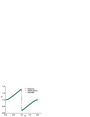
(a) 5th-order,$\lambda=1$

(b) 5th-order,$\lambda=10^{-3}$

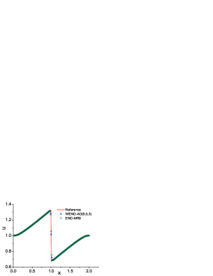
(c) 9th-order,$\lambda=1$

(d) 9th-order,$\lambda=10^{-3}$

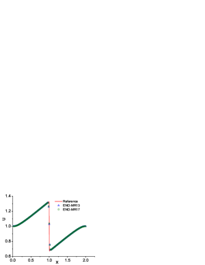
(e) 13th- and 17th- order,$\lambda=1$

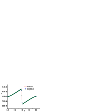
(f) 13th- and 17th- order,$\lambda=10^{-3}$

Figure 2: Solutions of the Burgers equation at $t=2/\lambda$ calculated by WENO-AO and ENO-MR schemes with $h=1/64$.

4.3 Numerical examples for the 1D Euler equations

We consider the 1D compressible Euler equations

$$\frac{\partial\mathbf{U}}{\partial t}+\frac{\partial\mathbf{F}}{\partial x}=0,$$ (29)

where $\mathbf{U}=[\rho,\rho u,\rho e]^{T}$ and $\mathbf{F}=[{\rho u,\rho u^{2}+p,(\rho e+p)u}]^{T}$ with $\rho$, $u$, $p$, and $e$ representing the density, velocity, pressure, and specific total energy respectively. The specific total energy is calculated as $e=\frac{p}{\rho(\gamma-1)}+\frac{1}{2}u^{2}$, where $\gamma$ is the specific heat ratio. Without particular instructions, $\gamma$ is set to 1.4 hereafter.

The first case is the Lax shock tube problem that is used to test the shock-capturing capability of numerical methods. The computational domain is [0,2], and the initial condition is given by

$$(\rho,u,p)=\begin{cases}(0.445,0.698,3.528),&\mbox{if }x<1\\ (0.5,0,0.571),&\mbox{otherwise}.\end{cases}$$

Non-reflection boundary conditions are applied to the left and right boundaries. Fig. 3 shows the density and velocity profiles at $t=0.26$ calculated by WENO-AO and ENO-MR schemes with $h=1/100$. We observe that both WENO-AO and ENO-MR schemes can capture discontinuity very well. Even when the designed order increases to a very high level, ENO-MR can still keep ENO properties.

(a) 5th-order

(b) 9th-order

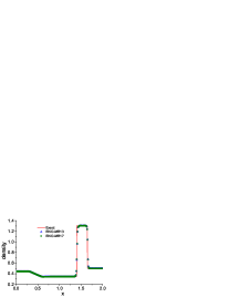
(c) 13th- and 17th-order

Figure 3: Density profiles of Lax shock tube problem at $t=0.26$ calculated by WENO-AO and ENO-MR schemes with $h=1/100$.

The second case is the Titarev and Toro Titarev and Toro (2004) problem which is an upgraded version of the Shu-Osher problem Shu and Osher (1988). It depicts the interaction of a Mach 1.1 moving shock with a very high-frequency entropy sine wave. The computational domain is [-5,5], and the initial condition is given by

$$(\rho,u,p)=\begin{cases}(1.515695,0.523346,1.805),&\mbox{if }x<-4.5\\ (1+0.1\mbox{sin}(20\pi x),0,1),&\mbox{otherwise}.\end{cases}$$

Non-reflection boundary conditions are applied to the left and right sides. Fig. 4 shows the density profiles in the high-frequency region at $t=5$ calculated by WENO-AO and ENO-MR schemes with $h=1/150$. The reference solution is calculated by the matured WENO-Z5 scheme with $h=1/1000$. We observe that WENO-AO(5,3) and ENO-MR5 perform similarly. ENO-MR9 performs much better than WENO-AO(9,5,3). ENO-MR13 and ENO-MR17 have no obvious advantage over ENO-MR9 at the current resolution.

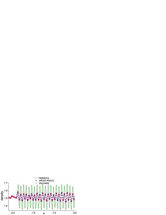
(a) 5th-order

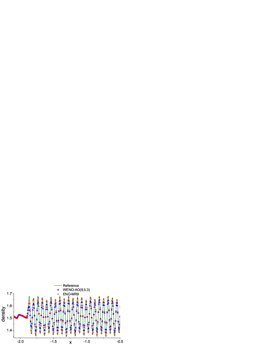
(b) 9th-order

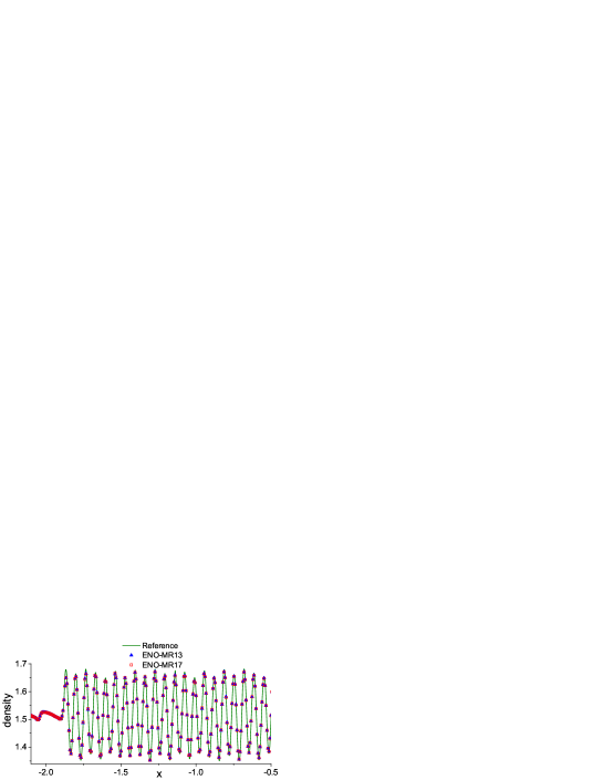
(c) 13th- and 17th-order

Figure 4: Density profiles of Titarev-Toro problem at $t=5$ calculated by WENO-AO and ENO-MR schemes with $h=1/150$.

4.4 Numerical examples for the 2D Euler equations

The 2D compressible Euler equations can be written as

$$\frac{\partial\mathbf{U}}{\partial t}+\frac{\partial\mathbf{F}}{\partial x}+\frac{\partial\mathbf{G}}{\partial y}=0,$$ (30)

with $\mathbf{U}=[\rho,\rho u,\rho v,\rho e]^{T}$, $\mathbf{F}=[{\rho u,\rho u^{2}+p,\rho uv,(\rho e+p)u}]^{T}$, and $\mathbf{G}=[{\rho v,\rho uv,\rho v^{2}+p,(\rho e+p)v}]^{T}$, where $\rho$, $u$, $v$, $p$, and $e$ denote the density, $x$-velocity, $y$-velocity, pressure, and specific total energy respectively. The specific total energy is calculated as $e=\frac{p}{\rho(\gamma-1)}+\frac{1}{2}(u^{2}+v^{2})$.

4.4.1 Two-dimensional Riemann problems

The computational is initially separated into four parts which are filled with gases of different states. We can simulate abundant interactions of different waves in two-dimensional space by providing different initial conditions. In this study, we consider two typical configurations. The first configuration is given by

$$\left(\rho,u,v,p\right)=\begin{cases}\left(0.138,1.206,1.206,0.029\right),&\text{in }[-1,0]\times[-1,0],\\ \left(0.5323,1.206,0,0.3\right),&\text{in }[-1,0]\times[0,1],\\ \left(1.5,0,0,1.5\right),&\text{in }[0,1]\times[0,1],\\ \left(0.5323,0,1.206,0.3\right),&\text{in }[0,1]\times[-1,0],\end{cases}$$

which depicts interactions of two horizontally moving shocks and two vertically moving shocks. The collision of the four normal shocks will result in two double-Mach reflections and an oblique shock moving along the diagonal of the computational domain. Fig. 5 shows density contours at $t=1$ calculated by WENO-AO and ENO-MR schemes with $801\times 801$ mesh points. At the current resolution, WENO-AO schemes start to trace out Kelvin-Helmholtz (KH) instabilities along the slip lines, but ENO-MR schemes can clearly capture more details.

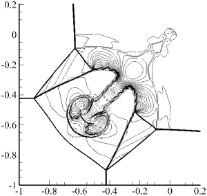
(a) WENO-AO(5,3)

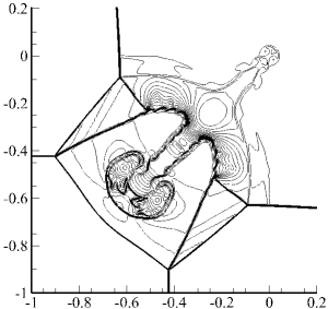
(b) WENO-AO(9,5,3)

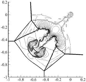
(c) ENO-MR5

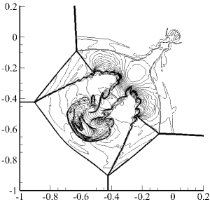
(d) ENO-MR9

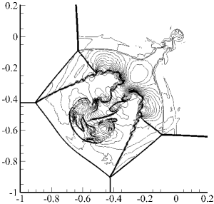
(e) ENO-MR13

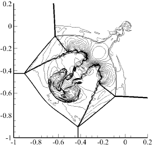
(f) ENO-MR17

Figure 5: Density contours of the first 2D Riemann problem at $t=1$ calculated by WENO-AO and ENO-MR schemes with $801\times 801$ mesh points. The contours contain 30 equidistant contours from 0.2 to 1.7.

The second configuration starts with four contact discontinuities formulated by

$$\left(\rho,u,v,p\right)=\begin{cases}\left(1,-0.75,0.5,1\right),&\text{in }[-1,0]\times[-1,0],\\ \left(2,0.75,0.5,1\right),&\text{in }[-1,0]\times[0,1],\\ \left(1,0.75,-0.5,1\right),&\text{in }[0,1]\times[0,1],\\ \left(3,-0.75,-0.5,1\right),&\text{in }[0,1]\times[-1,0].\end{cases}$$

Fig. 6 shows density contours at $t=1$ calculated by WENO-AO and ENO-MR schemes with $801\times 801$ mesh points. WENO-AO and ENO-MR schemes can capture the large-scale vortex at the center of the domain, but ENO-MR schemes capture many small-scale vortices along contact discontinuities which are almost absent in the results of WENO-AO schemes at the current resolution.

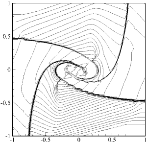
(a) WENO-AO(5,3)

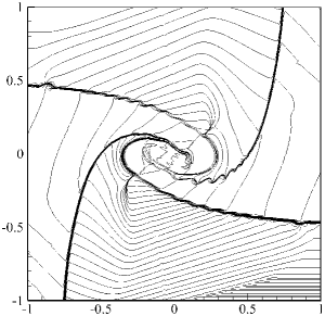
(b) WENO-AO(9,5,3)

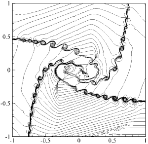
(c) ENO-MR5

(d) ENO-MR9

(e) ENO-MR13

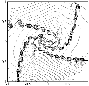
(f) ENO-MR17

Figure 6: Density contours of the second 2D Riemann problem at $t=1$ calculated by WENO-AO and ENO-MR schemes with $801\times 801$ mesh points. The contours contain 30 equidistant contours from 0.2 to 3.

4.4.2 Double Mach reflection problem

This case simulates the reflection of an oblique strong shock impacting on a plate which was originally proposed by Woodward and Colella Woodward and Colella (1984) and became a benchmark to test the shock-capturing capability and high fidelity of high-order schemes. The computational domain is $[0,4]\times[0,1]$, and the initial condition is given as

$$\left(\rho,u,v,p\right)=\begin{cases}\left(1.4,0,0,1\right)&\text{if }x>\frac{1}{6}+\frac{y}{\sqrt{3}},\\ \left(8,8.25sin(60^{\circ}),-8.25cos(60^{\circ}),116.5\right),&\text{otherwise},\end{cases}$$

which describes a Mach 10 oblique shock inclined at an angle of $60^{\circ}$ to the horizontal direction. The post-shocked states are imposed on the left boundary; Nonreflective boundary conditions are implemented on the right boundary; The exact motion of the oblique shock is imposed on the top boundary; Nonreflective and reflective boundary conditions are respectively imposed on the bottom boundary for $x\leq\frac{1}{6}$ and $x>\frac{1}{6}$. Fig. 7 and Fig. 8 respectively show the entire view and the enlarged view of the density contours at $t=0.2$ calculated by WENO-AO and ENO-MR schemes with $1201\times 301$ mesh points. All schemes capture the incident shock and reflected shock very well, but ENO-MR schemes capture more details of the small vortices in the reflection zone.

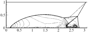
(a) WENO-AO(5,3)

(b) WENO-AO(9,5,3)

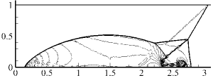
(c) WENO-MR5

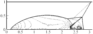
(d) WENO-MR9

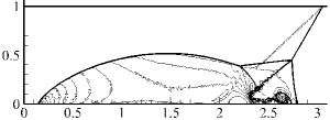
(e) WENO-MR13

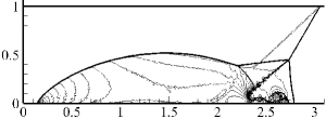
(f) WENO-MR17

Figure 7: Density contours of the double Mach reflection problem at $t=0.2$ calculated by WENO-AO and ENO-MR schemes with $1201\times 301$ mesh points. The density contours contain 40 equidistant contours from 2 to 21.

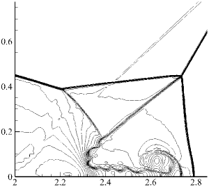
(a) WENO-AO(5,3)

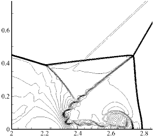
(b) WENO-AO(9,5,3)

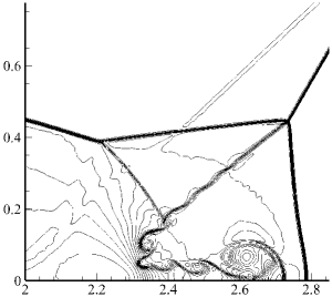
(c) ENO-MR5

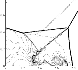
(d) ENO-MR9

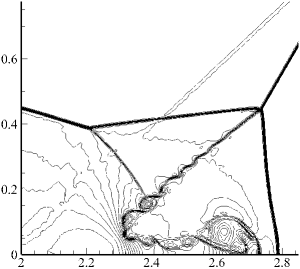
(e) ENO-MR13

(f) ENO-MR17

Figure 8: Enlarged view of density contours of the double Mach reflection problem at $t=0.2$ calculated by WENO-AO and ENO-MR schemes with $1201\times 301$ mesh points. The density contours contain 40 equidistant contours from 2 to 21.

4.4.3 Rayleigh-Taylor instability

Rayleigh-Taylor instability problem is another benchmark that was widely used to test the high-fidelity properties of high-order numerical schemes. Following the setup of Shi et al. Shi et al. (2003), the source term $\mathbf{S}=[0,0,\rho,\rho v]^{T}$ is added to the right hand side of the 2D Euler euqations, Eq. (30). The computational domain is $[0,0.25]\times[0,1]$, the ratio of specific heats $\gamma=5/3$, and the initial condition is given by

$$\left(\rho,u,v,p\right)=\begin{cases}\left(2,0,-0.025\sqrt{\frac{\gamma p}{\rho}}cos(8\pi x),2y+1\right)&\text{if }y<0.5,\\ \left(1,0,-0.025\sqrt{\frac{\gamma p}{\rho}}cos(8\pi x),y+1.5\right),&\text{otherwise}.\end{cases}$$

The development of Rayleigh-Taylor instabilities will induce complex fingering structures which are sensitive to small numerical errors. Low-dissipation schemes easily lose symmetry which can be fixed by carefully implementing the computer programs Fleischmann et al. (2019). In this study, we enforce the symmetry by a simple strategy from Wang et al. (2020). Fig. 9 shows the density contours at $t=1.95$ calculated by WENO-AO and ENO-MR schemes with $129\times 513$ and $201\times 801$ mesh points respectively. We observe that ENO-MR schemes capture much more details than WENO-AO schemes under the same grid resolution. High-order ENO-MR schemes also perform better than the ENO-MR5 scheme in this case.

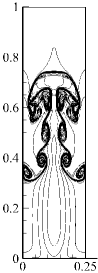
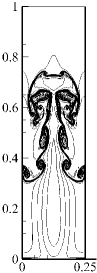
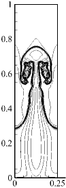
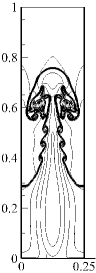
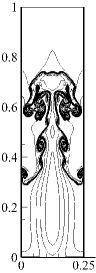
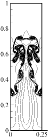
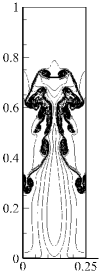
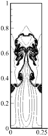
Figure 9: Density contours of the Rayleigh-Taylor instability problem at $t=1.95$ calculated by WENO-AO and ENO-MR schemes with $129\times 513$ (top row) and $201\times 801$ mesh points (bottom row). The results of WENO-AO(5,3), WENO-AO(9,5,3), ENO-MR5, ENO-MR9, ENO-MR13, ENO-MR17 schemes are arranged from left to right. The density contours contain 20 equidistant contours from 0.9 to 2.2.

4.4.4 Computational costs for two-dimensional tests

Table 9: Normalized computational costs of WENO-AO and ENO-MR schemes for different cases.

test	WENO-AO(5,3)	WENO-AO(9,5,3)	ENO-MR5	ENO-MR9	ENO-MR13	ENO-MR17
RP1	1	1.86	0.62	1.09	1.62	2.21
RP2	1	1.90	0.62	1.05	1.62	2.17
DMR	1	1.86	0.58	1.02	1.59	2.30
RTI128	1	1.82	0.55	0.84	1.20	1.68
RTI200	1	1.87	0.55	0.81	1.35	1.72

To roughly test the efficiency of the proposed ENO-MR schemes, we record the normalized computational costs of WENO-AO and ENO-MR schemes for the first Riemann problem (RP1), the second Riemann problem (RP2), the double Mach reflection (DMR), and the Rayleigh-Taylor instability (RTI) in Table 9. The computational costs are empirically determined by the parallel runtime of C codes using 16 CPU cores. We observe that ENO-MR schemes are more efficient than WENO-AO schemes of the same order. The computational costs of ENO-MR9 are similar to those of WENO-AO(5,3), although ENO-MR9 has much more candidate stencils. Even for the very high-order ENO-MR schemes, the computational costs are still affordable. The high efficiency of ENO-MR schemes benefits from two aspects: First, smoothness indicators of ENO-MR schemes are simple; Second, we directly use high-order stencils to reconstruct fluxes in smooth regions, and do not need to calculate smoothness indicators of remaining stencils. The second aspect is also why the relative computational costs of ENO-MR schemes have obvious fluctuations, because the proportion of smooth regions is different for different problems.

5 Conclusions

We construct a class of ENO-MR schemes with increasingly high-order based on linearly stable candidate stencils of unequal sizes by using simple smoothness indicators and an efficient selection strategy. The candidate stencils range from first-order up to the designed very high-order, and the proposed ENO-MR schemes can adaptively select the optimal stencil according to the simple smoothness indicators. Analysis and plenty of numerical examples show that the constructed ENO-MR schemes achieve optimal order in smooth regions while maintaining oscillation-free near strong discontinuities. Additionally, ENO-MR schemes are more accurate and more efficient than WENO-AO schemes, particularly for the instabilities of contact discontinuities. In conclusion, ENO-MR schemes provide an efficient way to construct high-order schemes with multi-resolution.

References

- Harten et al. [1987] Ami Harten, Bjorn Engquist, Stanley Osher, and Sukumar R Chakravarthy. Uniformly high order accurate essentially non-oscillatory schemes, III. Journal of Computational Physics, 71(2):231–303, 1987. doi:10.1016/0021-9991(87)90031-3.
- Shu and Osher [1988] Chi-Wang Shu and Stanley Osher. Efficient implementation of essentially non-oscillatory shock-capturing schemes. Journal of Computational Physics, 77:439–471, 1988.
- Shu and Osher [1989] Chi-Wang Shu and Stanley Osher. Efficient implementation of essentially non-oscillatory shock-capturing schemes, ii. Journal of Computational Physics, 83:32–78, 1989.
- Liu et al. [1994] Xu-Dong Liu, Stanley Osher, Tony Chan, et al. Weighted essentially non-oscillatory schemes. Journal of computational physics, 115(1):200–212, 1994.
- Jiang and Shu [1996] Guang-Shan Jiang and Chi-Wang Shu. Efficient implementation of weighted ENO schemes. Journal of Computational Physics, 126(1):202–228, 1996. doi:10.1006/jcph.1996.0130.
- Henrick et al. [2005] Andrew K Henrick, Tariq D Aslam, and Joseph M Powers. Mapped weighted essentially non-oscillatory schemes: achieving optimal order near critical points. Journal of Computational Physics, 207(2):542–567, 2005.
- Borges et al. [2008] Rafael Borges, Monique Carmona, Bruno Costa, and Wai Sun Don. An improved weighted essentially non-oscillatory scheme for hyperbolic conservation laws. Journal of Computational Physics, 227(6):3191–3211, 2008.
- Yamaleev and Carpenter [2009a] Nail K Yamaleev and Mark H Carpenter. Third-order energy stable WENO scheme. Journal of Computational Physics, 228(8):3025–3047, 2009a.
- Yamaleev and Carpenter [2009b] Nail K Yamaleev and Mark H Carpenter. A systematic methodology for constructing high-order energy stable WENO schemes. Journal of Computational Physics, 228(11):4248–4272, 2009b.
- Hu et al. [2010] XY Hu, Q Wang, and Nikolaus A Adams. An adaptive central-upwind weighted essentially non-oscillatory scheme. Journal of Computational Physics, 229(23):8952–8965, 2010.
- Fu et al. [2016] Lin Fu, Xiangyu Y Hu, and Nikolaus A Adams. A family of high-order targeted ENO schemes for compressible-fluid simulations. Journal of Computational Physics, 305:333–359, 2016.
- Fu et al. [2017] Lin Fu, Xiangyu Y Hu, and Nikolaus A Adams. Targeted ENO schemes with tailored resolution property for hyperbolic conservation laws. Journal of Computational Physics, 349:97–121, 2017.
- Fu et al. [2018] Lin Fu, Xiangyu Y Hu, and Nikolaus A Adams. A new class of adaptive high-order targeted ENO schemes for hyperbolic conservation laws. Journal of Computational Physics, 374:724–751, 2018.
- Fu [2021] Lin Fu. Very-high-order TENO schemes with adaptive accuracy order and adaptive dissipation control. Computer Methods in Applied Mechanics and Engineering, 387:114193, 2021.
- Fu [2023] Lin Fu. Review of the high-order TENO schemes for compressible gas dynamics and turbulence. Archives of Computational Methods in Engineering, 30(4):2493–2526, 2023.
- Balsara and Shu [2000] Dinshaw S Balsara and Chi-Wang Shu. Monotonicity preserving weighted essentially non-oscillatory schemes with increasingly high order of accuracy. Journal of Computational Physics, 160(2):405–452, 2000.
- Suresh and Huynh [1997] A Suresh and HT Huynh. Accurate monotonicity-preserving schemes with Runge–Kutta time stepping. Journal of Computational Physics, 136(1):83–99, 1997.
- Gerolymos et al. [2009] GA Gerolymos, D Sénéchal, and I Vallet. Very-high-order WENO schemes. Journal of Computational Physics, 228(23):8481–8524, 2009.
- Wu et al. [2021] Conghai Wu, Ling Wu, Hu Li, and Shuhai Zhang. Very high order WENO schemes using efficient smoothness indicators. Journal of Computational Physics, 432:110158, 2021.
- Wu et al. [2020] Conghai Wu, Ling Wu, and Shuhai Zhang. A smoothness indicator constant for sine functions. Journal of Computational Physics, 419:109661, 2020.
- Deng and Zhang [2000] Xiaogang Deng and Hanxin Zhang. Developing high-order weighted compact nonlinear schemes. Journal of Computational Physics, 165(1):22–44, 2000.
- Bianco et al. [1999] Franca Bianco, Gabriella Puppo, and Giovanni Russo. High-order central schemes for hyperbolic systems of conservation laws. SIAM Journal on Scientific Computing, 21(1):294–322, 1999.
- Levy et al. [1999] Doron Levy, Gabriella Puppo, and Giovanni Russo. Central WENO schemes for hyperbolic systems of conservation laws. ESAIM: Mathematical Modelling and Numerical Analysis, 33(3):547–571, 1999.
- Levy et al. [2000a] Doron Levy, Gabriella Puppo, and Giovanni Russo. A third order central WENO scheme for 2D conservation laws. Applied Numerical Mathematics, 33(1):415–422, 2000a.
- Pirozzoli [2002] Sergio Pirozzoli. Conservative hybrid compact-WENO schemes for shock-turbulence interaction. Journal of Computational Physics, 178(1):81–117, 2002.
- Ren and Zhang [2003] Yu-Xin Ren and Hanxin Zhang. A characteristic-wise hybrid compact-weno scheme for solving hyperbolic conservation laws. Journal of Computational Physics, 192(2):365–386, 2003.
- Qiu and Shu [2004] Jianxian Qiu and Chi-Wang Shu. Hermite WENO schemes and their application as limiters for Runge–Kutta discontinuous Galerkin method: One-dimensional case. Journal of Computational Physics, 193(1):115–135, 2004.
- Qiu and Shu [2005] Jianxian Qiu and Chi-Wang Shu. Hermite WENO schemes and their application as limiters for Runge–Kutta discontinuous Galerkin method II: Two-dimensional case. Computers & Fluids, 34(6):642–663, 2005.
- Titarev and Toro [2002] Vladimir A Titarev and Eleuterio F Toro. ADER: Arbitrary high order Godunov approach. Journal of Scientific Computing, 17(1-4):609–618, 2002.
- Titarev and Toro [2004] Vladimir A Titarev and Eleuterio F Toro. Finite-volume weno schemes for three-dimensional conservation laws. Journal of Computational Physics, 201(1):238–260, 2004.
- Balsara et al. [2013] Dinshaw S Balsara, Chad Meyer, Michael Dumbser, Huijing Du, and Zhiliang Xu. Efficient implementation of ADER schemes for Euler and magnetohydrodynamical flows on structured meshes–speed comparisons with Runge–Kutta methods. Journal of Computational Physics, 235:934–969, 2013. doi:10.1016/j.jcp.2012.04.051.
- Dumbser et al. [2008] Michael Dumbser, Dinshaw S Balsara, Eleuterio F Toro, and Claus-Dieter Munz. A unified framework for the construction of one-step finite volume and discontinuous Galerkin schemes on unstructured meshes. Journal of Computational Physics, 227(18):8209–8253, 2008. doi:10.1016/j.jcp.2008.05.025.
- Dumbser and Zanotti [2009] Michael Dumbser and Olindo Zanotti. Very high order schemes on unstructured meshes for the resistive relativistic MHD equations. Journal of Computational Physics, 228(18):6991–7006, 2009.
- Dumbser [2010] Michael Dumbser. Arbitrary high order schemes on unstructured meshes for the compressible Navier–Stokes equations. Computers & Fluids, 39(1):60–76, 2010.
- Shu [2009] Chi-Wang Shu. High order weighted essentially nonoscillatory schemes for convection dominated problems. SIAM review, 51(1):82–126, 2009.
- Shu [2016] Chi-Wang Shu. High order WENO and DG methods for time-dependent convection-dominated PDEs: A brief survey of several recent developments. Journal of Computational Physics, 316:598–613, 2016.
- Levy et al. [2000b] Doron Levy, Gabriella Puppo, and Giovanni Russo. Compact central WENO schemes for multidimensional conservation laws. SIAM Journal on Scientific Computing, 22(2):656–672, 2000b.
- Puppo et al. [2022] Gabriella Puppo, Matteo Semplice, and Giuseppe Visconti. Quinpi: integrating conservation laws with CWENO implicit methods. Communications on Applied Mathematics and Computation, pages 1–27, 2022.
- Semplice et al. [2016] Matteo Semplice, Armando Coco, and Giovanni Russo. Adaptive mesh refinement for hyperbolic systems based on third-order compact WENO reconstruction. Journal of Scientific Computing, 66(2):692–724, 2016.
- Semplice et al. [2021] Matteo Semplice, Elena Travaglia, and Gabriella Puppo. One-and multi-dimensional CWENOZ reconstructions for implementing boundary conditions without ghost cells. Communications on Applied Mathematics and Computation, pages 1–27, 2021.
- Semplice and Visconti [2020] Matteo Semplice and Giuseppe Visconti. Efficient implementation of adaptive order reconstructions. Journal of Scientific Computing, 83(1):1–27, 2020.
- Dumbser et al. [2017] Michael Dumbser, Walter Boscheri, Matteo Semplice, and Giovanni Russo. Central weighted ENO schemes for hyperbolic conservation laws on fixed and moving unstructured meshes. SIAM Journal on Scientific Computing, 39(6):A2564–A2591, 2017.
- Cravero and Semplice [2016] Isabella Cravero and Matteo Semplice. On the accuracy of WENO and CWENO reconstructions of third order on nonuniform meshes. Journal of Scientific Computing, 67(3):1219–1246, 2016.
- Cravero et al. [2018a] Isabella Cravero, Gabriella Puppo, Matteo Semplice, and Giuseppe Visconti. CWENO: uniformly accurate reconstructions for balance laws. Mathematics of Computation, 87(312):1689–1719, 2018a.
- Cravero et al. [2018b] Isabella Cravero, Gabriella Puppo, Matteo Semplice, and Giuseppe Visconti. Cool WENO schemes. Computers & Fluids, 169:71–86, 2018b.
- Cravero et al. [2019] Isabella Cravero, Matteo Semplice, and Giuseppe Visconti. Optimal definition of the nonlinear weights in multidimensional central WENOZ reconstructions. SIAM Journal on Numerical Analysis, 57(5):2328–2358, 2019.
- Zhu and Qiu [2016] Jun Zhu and Jianxian Qiu. A new fifth order finite difference WENO scheme for solving hyperbolic conservation laws. Journal of Computational Physics, 318:110–121, 2016.
- Zhu and Shu [2018] Jun Zhu and Chi-Wang Shu. A new type of multi-resolution WENO schemes with increasingly higher order of accuracy. Journal of Computational Physics, 375:659–683, 2018.
- Zhu and Shu [2019] Jun Zhu and Chi-Wang Shu. A new type of multi-resolution WENO schemes with increasingly higher order of accuracy on triangular meshes. Journal of Computational Physics, 392:19–33, 2019.
- Zhu and Shu [2020] Jun Zhu and Chi-Wang Shu. A new type of third-order finite volume multi-resolution WENO schemes on tetrahedral meshes. Journal of Computational Physics, 406:109212, 2020.
- Balsara et al. [2016] Dinshaw S Balsara, Sudip Garain, and Chi-Wang Shu. An efficient class of WENO schemes with adaptive order. Journal of Computational Physics, 326:780–804, 2016.
- Balsara et al. [2020] Dinshaw S Balsara, Sudip Garain, Vladimir Florinski, and Walter Boscheri. An efficient class of weno schemes with adaptive order for unstructured meshes. Journal of Computational Physics, 404:109062, 2020.
- Shen [2021] Hua Shen. An alternative reconstruction for WENO schemes with adaptive order. arXiv preprint arXiv:2103.12273, 2021.
- Shen et al. [2022] Hua Shen, Rasha Al Jahdali, and Matteo Parsani. A class of high-order weighted compact central schemes for solving hyperbolic conservation laws. Journal of Computational Physics, 466:111370, 2022.
- Shen [2023] Hua Shen. A class of ENO schemes with adaptive order for solving hyperbolic conservation laws. Computers & Fluids, 226:106050, 2023.
- Arbogast et al. [2018] Todd Arbogast, Chieh-Sen Huang, and Xikai Zhao. Accuracy of WENO and adaptive order WENO reconstructions for solving conservation laws. SIAM Journal on Numerical Analysis, 56(3):1818–1847, 2018.
- Don and Borges [2013] Wai-Sun Don and Rafael Borges. Accuracy of the weighted essentially non-oscillatory conservative finite difference schemes. Journal of Computational Physics, 250:347–372, 2013.
- Wang et al. [2019] Yinghua Wang, Bao-Shan Wang, and Wai Sun Don. Generalized sensitivity parameter free fifth order WENO finite difference scheme with Z-type weights. Journal of Scientific Computing, 81:1329–1358, 2019.
- Don et al. [2022] Wai Sun Don, Run Li, Bao-Shan Wang, and Yinghua Wang. A novel and robust scale-invariant WENO scheme for hyperbolic conservation laws. Journal of Computational Physics, 448:110724, 2022.
- Castro et al. [2011] Marcos Castro, Bruno Costa, and Wai Sun Don. High order weighted essentially non-oscillatory WENO-Z schemes for hyperbolic conservation laws. Journal of Computational Physics, 230(5):1766–1792, 2011.
- Butcher [2006] John C Butcher. General linear methods. Acta Numerica, 15:157–256, 2006.
- Gottlieb et al. [2001] Sigal Gottlieb, Chi-Wang Shu, and Eitan Tadmor. Strong stability-preserving high-order time discretization methods. SIAM review, 43(1):89–112, 2001.
- Gottlieb and Gottlieb [2003] Sigal Gottlieb and Lee-Ad J Gottlieb. Strong stability preserving properties of Runge–Kutta time discretization methods for linear constant coefficient operators. Journal of Scientific Computing, 18:83–109, 2003.
- Gottlieb [2005] Sigal Gottlieb. On high order strong stability preserving Runge-Kutta and multi step time discretizations. Journal of scientific computing, 25:105–128, 2005.
- Woodward and Colella [1984] Paul Woodward and Phillip Colella. The numerical simulation of two-dimensional fluid flow with strong shocks. Journal of computational physics, 54(1):115–173, 1984.
- Shi et al. [2003] Jing Shi, Yong-Tao Zhang, and Chi-Wang Shu. Resolution of high order WENO schemes for complicated flow structures. Journal of Computational Physics, 186(2):690–696, 2003.
- Fleischmann et al. [2019] Nico Fleischmann, Stefan Adami, and Nikolaus A Adams. Numerical symmetry-preserving techniques for low-dissipation shock-capturing schemes. Computers & Fluids, 189:94–107, 2019.
- Wang et al. [2020] Bao-Shan Wang, Wai Sun Don, Naveen K Garg, and Alexander Kurganov. Fifth-order A-WENO finite-difference schemes based on a new adaptive diffusion central numerical flux. SIAM Journal on Scientific Computing, 42(6):A3932–A3956, 2020.