Adjusted inference for multiple testing procedure in group sequential designs

Abstract

Adjustment of statistical significance levels for repeated analysis in group sequential trials has been understood for some time. Similarly, methods for adjustment accounting for testing multiple hypotheses are common. There is limited research on simultaneously adjusting for both multiple hypothesis testing and multiple analyses of one or more hypotheses. We address this gap by proposing adjusted-sequential p-values that reject an elementary hypothesis when its adjusted-sequential p-values are less than or equal to the family-wise Type I error rate (FWER) in a group sequential design. We also propose sequential p-values for intersection hypotheses as a tool to compute adjusted sequential p-values for elementary hypotheses. We demonstrate the application using weighted Bonferroni tests and weighted parametric tests, comparing adjusted sequential p-values to a desired FWER for inference on each elementary hypothesis tested.

1 Introduction

Recent decades have witnessed an increasing trend to answer multiple clinical questions within a single trial while strictly controlling Type I error for all statistical testing performed. Clinical questions may be related to hypotheses concerning multiple populations; in oncology, this can particularly be related to disease type or biomarkers that may be predictive of treatment effectiveness. Trials may also assess multiple experimental arms versus a common control. These efforts result in increasing complexity to adjust for multiplicity in the statistical framework. In addition, modern clinical trials are often designed in an adaptive way to allow using data accumulated in the trial to modify the trial’s course. Group sequential design (GSD) has been one of the most widely used adaptive designs, in which multiple analyses (i.e., interim and final analyses) may be conducted according to pre-determined rules to enable decisions. Existing literature on multiplicity and GSD focuses on either adjusting multiple hypotheses in a fixed design or adjusting multiple analyses in GSD with a single hypothesis. There is limited research on simultaneously adjusting for both multiple hypotheses and multiple analyses. We address this gap in this paper.

There are two approaches to adjust for multiplicity. One approach is to adjust the significance levels and compare the nominal p-values with corresponding adjusted significance levels. The other approach is to adjust the p-values and compare the adjusted p-values with the overall FWER(e.g., one-sided 0.025). For simple multiple testing procedures, these two approaches are often exchangeable. For example, to test $m$ equally weighted hypotheses using the Bonferroni procedure at the FWER $\alpha$, the adjusted significance level is $\alpha/m$ for each hypothesis and the adjusted p-value for hypothesis $H_{i}$ is $\min(1,mp_{i})$, where $p_{i}$ is the nominal p-value of hypothesis $H_{i}$. For more complicated multiple testing procedures, the adjusted p-value approach may be viewed as more straightforward and less confusing since we only need to compare the adjusted p-value of each individual hypothesis with a common benchmark, the FWER for the testing procedure. In this paper, we focus on the adjusted p-value approach. Below is a brief literature review on application of adjusted p-values for multiple testing in clinical trial settings.

For trials with a fixed design, the p-value of a single hypothesis is defined as the probability of obtaining a test statistic at least as extreme as observed under the null hypothesis. This is often called the unadjusted p-value or the nominal p-value. To test multiple hypotheses simultaneously, p-values need to be adjusted according to multiple test procedures to control FWER. Westfall and Young, (1993) provide a general definition of the adjusted p-value as the smallest significance level at which one would reject the hypothesis using the given multiple testing procedure. As illustrated above for the Bonferroni procedure, for most simple non-parametric or semi-parametric approaches, the calculation of multiplicity-adjusted p-values is fairly straightforward. For more complicated multiple testing procedures where the closed principle is followed (i.e., a hypothesis $H_{i}$ can be rejected if all intersection hypotheses containing $H_{i}$ are rejected (Marcus et al.,, 1976)), this definition can be applied as follows: assuming $p_{J}$, $J\subseteq\{1,...,m\}$, is the nominal p-value for intersection hypotheses $H_{J}$, the adjusted p-value for hypothesis $H_{i}$ is the largest p-value associated with the index set including $i$, i.e., $\max_{J:i\in J}p_{J}$ (Dmitrienko et al.,, 2009). Xi et al., (2017) applied this definition and provided a unified framework for a weighted parametric multiple testing procedure, in which the adjusted p-values can be calculated based on an analytic formula to avoid numerical root finding under multidimensional integration.

For trials with GSD, testing hypotheses at multiple analyses and the correlation among test statistics of interim analyses and final analyses adds a layer of complexity. For a single hypothesis with GSD, Liu and Anderson, 2008a defined the sequential p-value as the minimum significance level at which the hypothesis can be rejected at or before a given analysis time; this can be interpreted as the p-value adjusted for multiple analyses. For multiple hypotheses with GSD, Anderson et al., (2022) extended the framework of Xi et al., (2017) by considering the correlation structure among test statistics at interim and final analyses. However, their algorithm focused on the calculation of adjusted boundaries since no analytic formula can be easily provided for adjusted p-values as in Xi et al., (2017).

In this paper, we propose the adjusted-sequential p-value, which falls in the framework of the adjusted p-value approach. It is a p-value for each elementary hypothesis adjusted for both testing multiple hypotheses and multiple analyses. The rest of the paper is organized as follows. In Section 2, we articulate the definition of the proposed adjusted-sequential p-values. In Section 3, we present the implementation of adjusted-sequential p-values in both weighted Bonferroni and weighted parametric tests. Section 4 provides conclusions and discussion.

2 Multiple comparisons using p-values

Multiple hypotheses in clinical trials can be due to multiple treatment comparisons (e.g., multiple experimental treatment arms versus a common control), multiple populations (e.g., biomarker-positive versus an overall population of patients), and different endpoints (e.g., progression free survival [PFS] and overall survival [OS]). For notation, we denote the elementary hypotheses by $H_{1},H_{2},\ldots,H_{m}$ for some $m>0$. We also consider intersection hypothesis incorporating any non-empty subset of elementary hypotheses. That is, for any $\emptyset\neq J\subseteq I=\{1,2,\ldots,m\}$, we define $H_{J}=\cap_{j\in J}H_{j}.$ Controlling the family-wise Type I error $\alpha$ for all elementary hypotheses requires a closed-testing procedure evaluating tests of all $2^{m}-1$ intersection hypotheses (Marcus et al.,, 1976).

We investigate the above elementary/intersection hypotheses under group sequential designs with a total of $K$ analyses (including the final analysis). To test the $m$ elementary hypotheses at the $K$ analyses, we utilize the standardized multivariate normal test statistic as $Z_{i,k}$ with $i\in I$ and $k=1,2,\ldots,K$ as described in further detail in appendix D and Anderson et al., (2022). It is not necessary for all hypotheses to be evaluated at all analyses, but we assume a common number of analyses for each hypothesis here to simplify notation and presentation.

With the $mK$ test statistics $\{Z_{i,k}\}_{i\in I,k=1,\ldots,K}$, we can accept or reject the null hypothesis based on p-values. In multiple testing under group sequential designs, there are commonly four types of p-values.

Nominal p-value. The probability under the null hypothesis that the test statistic of an elementary hypothesis is at least as extreme as observed.

Repeated p-value. For an elementary hypothesis $H_{j}$ at analysis $k$, the repeated p-value is the minimum significance level that $H_{j}$ can be rejected at analysis $k$ (Jennison and Turnbull,, 2000):

$$p_{j,k}^{rep} = \inf\left\{\mu:Z_{j,k}\geq\widetilde{Z}_{j,k}(\mu)\right\},$$ (1)

where the boundary $\widetilde{Z}_{j,k}(\mu)$ is a function of $\mu\in(0,1)$ . Note that the repeated p-values require smoothness assumptions for group sequential bounds to enable the Bonferroni-based method of Maurer and Bretz, (2013).

Sequential p-value. For an elementary hypothesis $H_{j}$ at analysis $k$, the sequential p-value is the minimum significance level that $H_{j}$ can be rejected at or before analysis $k$:

$$p_{j,k}^{seq} = \inf\left\{\mu:\underbrace{\left\{Z_{j,1}\geq\widetilde{Z}_{j,1}(\mu)\right\}}_{\text{1st analysis}}\;\cup\;\underbrace{\left\{Z_{j,2}\geq\widetilde{Z}_{j,2}(\mu)\right\}}_{\text{2nd analysis}}\;\cup\;\ldots\;\cup\;\underbrace{\left\{Z_{j,k}\geq\widetilde{Z}_{j,k}(\mu)\right\}}_{k\text{-th analysis}}\right\}.$$ (2)

To ease computation, one can simplify the above definition as shown in Appendix A. In addition to the sequential p-value for an elementary hypothesis $H_{j}$, one can also get the sequential p-value for an intersection hypothesis $H_{J}$ as

$$p_{J,k}^{seq} = \inf\left\{\mu:\underbrace{\left\{Z_{j_{1},1}\geq\widetilde{Z}_{j_{1},1}(\mu,J)\right\}\;\cup\;\left\{Z_{j_{2},1}\geq\widetilde{Z}_{j_{2},1}(\mu,J)\right\}\;\cup\;\ldots\;\cup\;\left\{Z_{j_{L},1}\geq\widetilde{Z}_{j_{L},1}(\mu,J)\right\}}_{\text{1st analysis}}\right.$$

$$\;\cup\;\underbrace{\left\{Z_{j_{1},2}\geq\widetilde{Z}_{j_{1},2}(\mu,J)\right\}\;\cup\;\left\{Z_{j_{2},2}\geq\widetilde{Z}_{j_{2},2}(\mu,J)\right\}\;\cup\;\ldots\;\cup\;\left\{Z_{j_{L},2}\geq\widetilde{Z}_{j_{L},2}(\mu,J)\right\}}_{\text{2nd analysis}}$$

$$\left.\;\cup\;\ldots\cup\underbrace{\left\{Z_{j_{1},k}\geq\widetilde{Z}_{j_{1},k}(\mu,J)\right\}\;\cup\;\left\{Z_{j_{2},k}\geq\widetilde{Z}_{j_{2},k}(\mu,J)\right\}\;\cup\;\ldots\;\cup\;\left\{Z_{j_{L},k}\geq\widetilde{Z}_{j_{L},k}(\mu,J)\right\}}_{k\text{-th analysis}}\right\},$$

where $J=\{j_{1},j_{2},\ldots,j_{L}\}$ and $\widetilde{Z}_{j,k}(\mu,J)$ is the upper bound of the elementary hypothesis $H_{j}$ at the $k$-th analysis, which is decided by $\mu$ and the intersection set $J$.

To calculate the sequential p-value, we first compute the boundaries $\widetilde{Z}_{j,k}(\mu,J)$, which depends on the selection of the multiple test procedure. For example, weighted Bonferroni and WPGSD (see Section 3) are two procedures of the graphical approach (see a review in Appendix B) With the boundaries available, we use a root finding method to determine $\mu$ in (2) and (2).

Adjusted sequential p-value. For an elementary hypothesis $H_{j}$ at analysis $k$, the adjusted-sequential p-value is the maximum of the sequential p-values of all the intersection hypotheses containing $H_{j}$:

$$p_{j,k}^{aseq}=\max_{\{J:\;j\in J\}}p_{J,k}^{seq}.$$ (4)

The adjusted-sequential p-value of $H_{j}$ can be compared with the FWER (e.g., 0.025 one-sided); i.e., if the adjusted sequential p-value of $H_{j}$ is less than the FWER, then $H_{j}$ can be rejected.

One strength of the adjusted-sequential p-value is its simplicity: users only need to compare an adjusted-sequential p-value for any individual hypothesis with the pre-specified FWER (say, 0.025). In this way, those interpreting the trial are no longer required to utilize many Z boundaries. In contrast, repeated p-values have varied benchmarks requiring users to compare with allocated alpha, which depends on other test results. In practice, users may not have comprehensive knowledge of the assigned $\alpha$-values over time, making the repeated p-value implementation challenging.

3 Implementation of adjusted-sequential p-values

The steps for computing the adjusted-sequential p-values are as outlined below.

• Step 1: Select the testing approach. Two approaches are discussed here.

  • The weighted Bonferroni test is simply illustrated, communicated, and implemented by the graphical approach (Bretz et al.,, 2009; Burman et al.,, 2009). For each elementary hypothesis $H_{j}$, we reject it if $p_{j}\leq w_{j}(I)\alpha$, where $p_{j}$ is the hyopothesis’ nominal p-value. When an elementary hypothesis $H_{j}$ is rejected, the graph and transition matrix is updated. Testing then proceeds with the reduced hypothesis set excluding $H_{j}$ and the updated weights. This reject, reallocate and reduce procedure continues until no remaining elementary hypothesis can be rejected. A comprehensive review is given in Bretz et al., (2009) and Maurer and Bretz, (2013).

  • WPGSD (weighted parametric group sequential design) test. Unlike the weighted Bonferroni test, the WPGSD takes into account the correlations between test statistics when evaluating multiple hypotheses in group sequential designs. This enables less stringent bounds while ensuring robust control of the FWER at the specified level $\alpha$. For a detailed examination, refer to the comprehensive review provided in (Anderson et al.,, 2022).

• Step 2: For analysis $k$, compute the sequential p-values through analyis $k$ of all possible intersection hypotheses using the formula in (2). We consider the interaction hypothesis $H_{J}$ as an example. Assuming a specified family-wise significance level $\mu$, we can compute the Z boundaries for each elementary hypothesis within $J$ by utilizing the spending function, weights, and chosen testing procedure (weighted Bonferroni or WPGSD). By comparing these Z boundaries with the observed Z statistics, we can reject $H_{J}$ if any observed Z statistic exceeds the respective Z boundary. We employ root-finding to identify the minimum significance level $\mu$ at which $H_{J}$ can be rejected. This identified root corresponds to the sequential p-value of $H_{J}$ at analysis $k$, as defined in (2).

• Step 3: Compute the adjusted sequential p-value for each elementary hypothesis $H_{j}$ by taking the maximum of all the sequential p-value of the intersection hypotheses containing $H_{j}$, as shown in (4).

• Step 4: Repeat Steps 2 and 3 for all analyses.

In Step 2, the procedure of computing Z boundaries is outlined in Maurer and Bretz, (2013) when the weighted Bonferroni method is chosen, and describled in Anderson et al., (2022) when the WPGSD method is selected. The following example demonstrates a detailed implementation of adjusted-sequential p-values. The code to reproduce the example results can be found at https://merck.github.io/wpgsd/articles/adj-seq-p.html.

Example 3.1

In a 2-arm controlled clinical trial example with one primary endpoint, there are 3 patient populations defined by the status of two biomarkers A and B: (i) the biomarker A positivepopulation, (ii) the biomarker B positive population, and (iii) the overall population. The 3 elementary hypotheses are:

• $H_{1}$: experimental treatment is superior to control in the biomarker A positive population;

• $H_{2}$: experimental treatment is superior to control in the biomarker B positive population;

• $H_{3}$: experimental treatment is superior to control in the overall population.

The study has one interim analysis and one final analysis and the number of events is listed in Table 1.

Table 1: Number of events in Example 1A.

Population Number of events at IA¹ Number of events at FA¹ Biomarker A positive 100 200 Biomarker B positive 110 220 Biomarker A B both positive 80 160 Overall population 225 450 1 IA, FA is short for interim and final analysis, respectively.

With the graphical approach review in Appendix B, we assign the initial weights of $H_{1},H_{2},H_{3}$ as $\left(w_{1}(I),w_{2}(I),w_{3}(I)\right)=(0.3,0.3,0.4).$ The multiplicity strategy is visualized in Figure 1. We can compute the weighting strategy for each intersection hypothesis in Table 3. If $H_{1}$ is rejected, then $3/7$ local significance level $\alpha_{1}$ will be propagated to $H_{2}$, and $4/7$ will go to $H_{3}$. If $H_{3}$ is rejected, then half of $\alpha_{3}$ goes to $H_{1}$, and half goes to $H_{2}$. Mathematically, its transition matrix is

$$G=\left(\begin{array}[]{ccc}0&3/7&4/7\\ 3/7&0&4/7\\ 1/2&1/2&0\\ \end{array}\right).$$

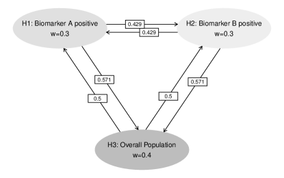
Figure 1: Graphical representation in Example 1A

Assume the nominal p-values of $H_{1},H_{2}$, and $H_{3}$ at IA are 0.02, 0.01, 0.012 at the interim analysis, and 0.015, 0.012, 0.01 at the final analysis. For the weighted Bonferroni approach, each hypothesis employs an Hwang-Shib-DeCani (HSD; $\gamma=-4$) $\alpha$-spending function. For the WPGSD method, we assume an HSD($\gamma=-4$) $\alpha$-spending function is used for overall $\alpha$ spending with minimum information fraction (i.e., Method 3(b) in Anderson et al., (2022)). Of note, the information fraction was 0.5 at the interim for all hypotheses given the number of events in Table 1. The correlation matrix of $\{Z_{j,k}\}_{j=1,\ldots,m;\;k=1,\ldots,K}$ is presented in Appendix D when using the WPGSD method. With the methods above, we derive the adjusted-sequential p-values in Table 2.

Table 2: The p-values via Weighted Bonferroni in Example 3.1

Hypothesis Weighted Bonferroni WPGSD sequential p-values adjusted-sequential p-values sequential p-values adjusted-sequential p-values Interim analysis $H_{1,2,3}$ 0.2097 - 0.1636 - $H_{1,2}$ 0.1678 - 0.1400 - $H_{1,3}$ 0.1468 - 0.1302 - $H_{2,3}$ 0.1468 - 0.1282 - $H_{1}$ 0.1258 0.2097 0.1258 0.1636 $H_{2}$ 0.0839 0.2097 0.0839 0.1636 $H_{3}$ 0.0839 0.2097 0.0839 0.1636 Final analysis $H_{1,2,3}$ 0.0266 - 0.0206 - $H_{1,2}$ 0.0255 - 0.0210 - $H_{1,3}$ 0.0186 - 0.0165 - $H_{2,3}$ 0.0186 - 0.0162 - $H_{1}$ 0.0159 0.0266 0.0159 0.0210 $H_{2}$ 0.0127 0.0266 0.0127 0.0210 $H_{3}$ 0.0106 0.0266 0.0106 0.0206

Results by weighted Bonferroni method. At the interim analysis, all the 3 adjusted-sequential p-values are greater than 0.025, so none are rejected. At the final analysis, all of them are larger than 0.025, and again no hypothesis is rejected. Besides the adjusted-sequential p-values, users can also apply the sequential p-values for individual and intersection hypotheses. Since consonance holds under weighted Bonferroni in group sequential designs (Maurer and Bretz,, 2013; Hommel et al.,, 2007) there is no need for testing intersection hypotheses. As indicated by Table 2, at the final analysis, the sequential p-values for $H_{1}$ amount to 0.0266, which exceeds $0.3\times 0.025=0.0075$ where $0.3$ represents the initial weight assigned to $H_{1}$. As a result, we cannot reject $H_{1}$. Similarly, $H_{2}$ and $H_{3}$ cannot be rejected because $0.0266>0.3\times 0.025=0.0075$ and $0.0266\geq 0.4\times 0.025=0.01$.

Results by WPGSD. Since the adjusted-sequential p-values at the interim analysis are all greater than 0.025, no hypotheses are rejected at that time. At the final analysis, all individual hypotheses are rejected since their adjusted-sequential p-values are all smaller than 0.025.

From the above example, we find the WPGSD method is more efficient than weighted Bonferroni since the sequential p-values for the intersection hypotheses are all smaller for WPGSD than weighted Bonferroni, which leads to more hypotheses being rejected. This is because the WPGSD accounts for the correlation between the test statistics, which can increase study power or save sample size, compared to procedures not accounting for the correlation. For the consumer of trial results (e.g., the data monitoring committee), the adjusted sequential p-values are immediately interpretable to understand which hypotheses are rejected.

4 Discussion

In multiple comparisons, there are two approaches to adjust for multiplicity. One approach is to adjust the significance levels to compare with nominal p-values observed. The other approach is to adjust the p-values and compare the adjusted p-values with the overall family-wise significance level for a trial (e.g., one-sided 0.025). In our previous work (Anderson et al.,, 2022), we considered adjusted significance levels. In this paper, we proposed the adjusted sequential p-value as a simple-to-interpret method to describe the outcome of testing of individual hypotheses in group sequential designs. That is, the adjusted sequential p-value for any individual hypothesis need only be compared with the FWER for the combined set of hypotheses being tested. This is an extension of similar methods for fixed designs in Xi et al., (2017). From the computational perspective, the adjusted p-value approach is easier than the adjusted significance level approach for the weighted parametric method in fixed design (i.e., no interim analysis) (Xi et al.,, 2017). However, this advantage cannot be extended to WPGSD. This is due to a need for interaction hypotheses since consonance for the WPGSD method which is not needed not ensured. For the weighted Bonferroni method, the consonance property holds and there is a short-cut as shown in Section 3 with a sequential p-value approach. While the computations for the adjusted sequential p-value are detailed, we have provided software in https://github.com/Merck/wpgsd. There are two alternatives to approach this testing problem:

1. The adjusted significance bound at each analysis for each hypothesis can be computed for all possible alpha levels at which each hypothesis can be tested in different intersection hypotheses (Anderson et al.,, 2022). With, for example, 3 hypotheses, 3 analyses, and 3 possible alpha levels, this is already 9 bounds that would be required prior to unblinding for analysis in order to cover all possible needed evaluations. While the standard group sequential computations required are straightforward, interpretation can be challenging for a Data Monitoring Committee (DMC). However, this can be very useful for checking rejections made with the adjusted sequential p-value method we propose here.

2. For weighted Bonferroni tests where no test correlations are accounted for, computing a sequential p-value for each hypothesis at each analysis can be a useful simplification. These sequential p-values can be plugged into a hypothesis graph as if no interim analyses were performed. Since the software is readily available for this in the gMCP R package, this is straightforward.

In this paper, we have extended the sequential p-value approach in a group sequential design from an elementary hypothesis as in Liu and Anderson, 2008b to intersection hypotheses and then to closed testing of individual hypotheses. Additionally, we provide the definition of the adjusted-sequential p-value for each elementary hypothesis. If the adjusted-sequential p-value of a hypothesis is less than the family-wise significance level, this hypothesis is rejected, whether at interim analyses or final analysis. We apply the aforementioned adjusted inference in the weighted Bonferroni method and the WPGSD method accounting for test correlations, with a graphical approach. The attraction of WPGSD is increased testing efficiency by accounting for known correlations between individual tests. The adjusted p-value approach simplifies evaluation for a DMC and complements previous literature which mostly uses the adjusted significance level approach (Anderson et al.,, 2022).

Appendix

Appendix A Simplification of sequential p-value

The sequential p-value of an elementary hypothesis $H_{j}$ at the $k$-th analysis can be simplified from (2) as

$$p_{j,k}^{seq} = \inf\left\{\mu:Z_{j,1}\geq\widetilde{Z}_{j,1}(\mu)\;\cup\;Z_{j,2}\geq\widetilde{Z}_{j,2}(\mu)\;\cup\;\ldots\;\cup\;Z_{j,k}\geq\widetilde{Z}_{j,k}(\mu)\right\}$$

$$= \sup\left\{\mu:\underset{1\leq k^{\prime}\leq k}{\cap}\{Z_{j,k^{\prime}}<\widetilde{Z}_{j,k^{\prime}}(\mu)\}\right\}$$

$$= \sup\left\{\mu:\underset{1\leq k^{\prime}\leq k}{\max}\{Z_{j,k^{\prime}}-\widetilde{Z}_{j,k^{\prime}}(\mu)\}<0\right\}.$$

With the above simplification, we can re-write the sequential p-values of an intersection hypothesis $H_{J}$ as

$$p_{J,k}^{seq} = \sup\left\{\mu:\max_{1\leq k^{\prime}\leq k,\;j\in J}\{Z_{j,k^{\prime}}-\widetilde{Z}_{j,k^{\prime}}(\mu,J)\}\leq 0\right\},$$

where $Z_{j,k^{\prime}}$ is the test statistic for the elementary hypothesis $H_{j}$ at the $k^{\prime}$-th analysis and $\widetilde{Z}_{j,k^{\prime}}(\mu,J)$ is the upper bound of the elementary hypothesis $H_{j}$ at the $k^{\prime}$-th analysis when tested at level $\mu$ in the intersection set $J$. We note this requires a $|J|$-variate normal computations which are not demonstrated here but are available in the software repository at https://github.com/Merck/wpgsd.

Appendix B Graphical hypothesis testing approach

This section introduces the graphical method and its weighting strategy. It is independently derived by Bretz et al., (2009) and Burman et al., (2009) for the multiplicity problem. Though the graphical representations and rejection algorithms in these two articles are different, the underlying ideas are closely related (Guilbaud and Karlsson,, 2011). Using the graphical approach of Bretz et al., (2009), the hypotheses $H_{1},H_{2},\ldots,H_{m}$ are represented by vertices with associated weights denoting the local significance levels $\alpha_{1},\alpha_{2},\ldots,\alpha_{m}$ with $\sum_{j=1}^{m}\alpha_{j}=\alpha,$ the FWER for all testing. We further denote $I=\{1,2,\ldots,m\}$ and $w_{j}=\alpha_{j}/\alpha,j=1,2,\ldots,m$. Any two vertices $H_{i}$ and $H_{j},1\leq i,j\leq m$ are connected through directed edges, where the associated weight $g_{ij}$ indicates the fraction of the (local) significance level $\alpha_{i}$ that is propagated to $H_{j}$ once $H_{i}$ (the hypothesis at the tail of the edge) has been rejected. A weight $g_{ij}=0$ indicates that no propagation of the significance level is foreseen and the edge is dropped for convenience. Generally, for any $i,j\in I$, we have $0\leq g_{ij}\leq 1$ and $\sum_{j=1}^{m}g_{ij}\leq 1$. We note $g_{ii}=0,i=1,2,\ldots,k$. The matrix $G=(g_{ij})\in\mathbb{R}^{m\times m}$ is referred to as the transition matrix.

For each $J\subseteq I$, there is a collection of weights $w_{j}(J)$ such that $0\leq w_{j}(J)\leq 1$ and $\sum_{j\in J}w_{j}(J)\leq 1$. Such $w_{j}(J)$ defines inference in the weighted Bonferroni test. Specifically, assume $p_{j}$ is the unadjusted p-value for $H_{j}$, then we reject $H_{J}$ if $p_{j}\leq w_{j}(J)\alpha$ for at least one $j\subseteq J$. Hommel et al., (2007) introduced a useful subclass of sequentially rejective Bonferroni-based closed test procedures. They showed that the monotonicity condition

$$w_{j}(J_{1})\leq w_{j}(J_{2}),\;\;\forall j\in J_{2}\subseteq J_{1}\subseteq J.$$

ensures consonance. A closed procedure is called consonant if the rejection of the complete intersection null hypothesis $H_{I}$ further implies that at least one elementary hypothesis $H_{j},(j\in I)$, can be rejected. This substantially simplifies the implementation and interpretation of related closed testing procedures, as the closure tree of $2^{m}-1$ intersection hypotheses is tested in only $m$ steps. In practice, consonance is a desirable property leading to shortcut procedures that give the same rejection decisions as the original closed procedure but with fewer operations (Xi et al.,, 2017).

From the above example, we find that, for a global null hypothesis $H_{I}$, its weighting strategies are formally defined by two components: (1) the weights of the elementary hypothesis is $w_{i}(I)$ for any $i\in I$, and (2) transition matrix $G$. For an intersection hypothesis $H_{J}$ with $\emptyset\neq J\subseteq I$, the weights of each elementary hypothesis are $w_{j}(J)$ for any $j\in J$, which can be derived by Algorithm 1 in Bretz et al., (2011).

Appendix C Weighting strategies of Example 3.1

The weighting strategy of Example 3.1 is shown in Table 3.

Table 3: Weighting strategy in Example 1A and 1B.

$H_{J}$ $w_{1}(J)$ $w_{2}(J)$ $w_{3}(J)$ $H_{1,2,3}$ 0.3 0.3 0.4 $H_{1,2}$ 0.5 0.5 - $H_{1,3}$ 0.3 - 0.7 $H_{2,3}$ - 0.3 0.7 $H_{1}$ 1 - - $H_{2}$ - 1 - $H_{3}$ - - 1 1 $H_{1,2,3}$ refers to the intersection hypothesis consisting $H_{1},H_{2}$ and $H_{3}$, i.e., $H_{1}\cap H_{2}\cap H_{3}$. Similar logic also applies to $H_{1,2},H_{1,3}$ and $H_{2,3}$.

Appendix D Correlated test statistics

As noted in Chen et al., (2021), the test statistics $\{Z_{i,k}\}_{i\in I,k=1,\ldots,K}$ are correlated via analysis time or overlapping populations or shared control arm:

$$\text{Corr}(Z_{i_{1},k_{1}},Z_{i_{2},k_{2}})=\frac{n_{i_{1}\wedge i_{2},k_{1}\wedge k_{2}}}{\sqrt{n_{i_{1},k_{1}}n_{i_{2},k_{2}}}}.$$

Here $n_{i,k}$ is the number of observations (or the number of events for time-to-event endpoints) collected cumulatively through analysis $k$ for elementary hypothesis $H_{i}$. And $n_{i_{1}\wedge i_{2},k_{1}\wedge k_{2}}$ is the number of observations (or events) included in both $Z_{i_{1},k_{1}}$ and $Z_{i_{2},k_{2}}$. The full correlation matrix of $\{Z_{i,k}\}_{i\in I,k=1,\ldots,K}$ ($mK\times mK$) can be derived this way and is referred to as the complete correlation structure (CCS) in Chen et al., (2021) and Anderson et al., (2022). In Example 3.1, we present a numerical example and show the explicate calculation of the CCS.

Example D.1

Following Example 3.1 with the number of events at the interim and the final analyses for each population in Table 1, we articulate the details of compute the correlation matrix as follows.

In the interim analysis, the correlation between $H_{1}$ and $H_{2}$ is $\text{Corr}(Z_{1,1},Z_{2,1})=\frac{64}{\sqrt{80\times 88}}$. The numerator is the number of events included in both $Z_{1,1},Z_{2,1}$, and the denominator are the number of events of $Z_{1,1},Z_{2,1}$, respectively. In the final analysis, the correlation between $H_{2}$ and $H_{3}$ is $\text{Corr}(Z_{2,2},Z_{3,2})=\frac{176}{\sqrt{176\times 360}}$. The numerator is the number of events included in both biomarker B positive and the overall population, and the denominator is the number of events of the two populations, respectively. The full correlation matrix in Table 4

Table 4: Correlation matrix of test statistics in Example 3.1.

$Z_{1,1}$ $Z_{2,1}$ $Z_{3,1}$ $Z_{1,2}$ $Z_{2,2}$ $Z_{3,2}$ $Z_{1,1}$ 1 $\frac{64}{\sqrt{80\times 88}}$ $\frac{80}{\sqrt{80\times 180}}$ $\frac{80}{\sqrt{80\times 160}}$ $\frac{64}{\sqrt{80\times 176}}$ $\frac{80}{\sqrt{80\times 360}}$ $Z_{2,1}$ 0.76 1 $\frac{88}{\sqrt{88\times 180}}$ $\frac{64}{\sqrt{88\times 160}}$ $\frac{88}{\sqrt{88\times 176}}$ $\frac{88}{\sqrt{88\times 360}}$ $Z_{3,1}$ 0.67 0.70 1 $\frac{80}{\sqrt{180\times 160}}$ $\frac{88}{\sqrt{180\times 176}}$ $\frac{180}{\sqrt{180\times 360}}$ $Z_{1,2}$ 0.71 0.54 0.47 1 $\frac{128}{\sqrt{160\times 176}}$ $\frac{160}{\sqrt{160\times 360}}$ $Z_{2,2}$ 0.54 0.71 0.49 0.76 1 $\frac{176}{\sqrt{176\times 360}}$ $Z_{3,2}$ 0.47 0.49 0.71 0.67 0.70 1

We acknowledge that, in some cases, the correlation among the hypotheses is only known for subsets of the hypotheses. For example, suppose there are 4 elementary hypotheses in a trial:

• $H_{1}$: PFS in the biomarker-positive population;

• $H_{2}$: PFS in the overall population;

• $H_{3}$: OS in the biomarker-positive population;

• $H_{4}$: OS in the overall population.

Based on the overlapping number of events, the correlation is known between hypotheses concerning the same endpoint (i.e., $H_{1}$ and $H_{2}$ for PFS, and $H_{3}$ and $H_{4}$ for OS), but not between hypotheses concerning different endpoints (e.g., $H_{1}$ and $H_{3}$, or $H_{1}$ and $H_{4}$). When the correlation between test statistics is partially known, we can partition $I$ into $l$ mutually exclusive subsets $I_{1},\ldots,I_{l}$ such that $I=\cup_{i=1}^{l}I_{i}$. For a test hypothesis $J\subseteq I$, let $J_{i}=J\cap I_{i}$ with $i=1,\ldots,l$. Since the correlation of $J_{i}$ is fully known, we can apply the aforementioned method for inference within that subset of the intersection hypothesis.

References

- Anderson et al., (2022) Anderson, K. M., Guo, Z., Zhao, J., and Sun, L. Z. (2022). A unified framework for weighted parametric group sequential design. Biometrical Journal.
- Bretz et al., (2009) Bretz, F., Maurer, W., Brannath, W., and Posch, M. (2009). A graphical approach to sequentially rejective multiple test procedures. Statistics in medicine, 28(4):586–604.
- Bretz et al., (2011) Bretz, F., Posch, M., Glimm, E., Klinglmueller, F., Maurer, W., and Rohmeyer, K. (2011). Graphical approaches for multiple comparison procedures using weighted bonferroni, simes, or parametric tests. Biometrical Journal, 53(6):894–913.
- Burman et al., (2009) Burman, C.-F., Sonesson, C., and Guilbaud, O. (2009). A recycling framework for the construction of bonferroni-based multiple tests. Statistics in Medicine, 28(5):739–761.
- Chen et al., (2021) Chen, T.-Y., Zhao, J., Sun, L., and Anderson, K. M. (2021). Multiplicity for a group sequential trial with biomarker subpopulations. Contemporary Clinical Trials, 101:106249.
- Dmitrienko et al., (2009) Dmitrienko, A., Tamhane, A. C., and Frank, B. (2009). Multiple Testing Problems in Pharmaceutical Statistics. Chapman and Hall/CRC, Florida.
- Guilbaud and Karlsson, (2011) Guilbaud, O. and Karlsson, P. (2011). Confidence regions for bonferroni-based closed tests extended to more general closed tests. Journal of Biopharmaceutical Statistics, 21(4):682–707.
- Hommel et al., (2007) Hommel, G., Bretz, F., and Maurer, W. (2007). Powerful short-cuts for multiple testing procedures with special reference to gatekeeping strategies. Statistics in Medicine, 26(22):4063–4073.
- Jennison and Turnbull, (2000) Jennison, C. and Turnbull, B. W. (2000). Group Sequential Methods with Applications to Clinical Trials. Chapman and Hall/CRC, Boca Raton, FL.
- (10) Liu, Q. and Anderson, K. M. (2008a). On adaptive extensions of group sequential trials for clinical investigations. Journal of the American Statistical Association, 103(484):1621–1630.
- (11) Liu, Q. and Anderson, K. M. (2008b). On adaptive extensions of group sequential trials for clinical investigations. Journal of the American Statistical Association, 103:1621–1630.
- Marcus et al., (1976) Marcus, R., Peritz, E., and Gabriel, K. R. (1976). On closed testing procedures with special reference to ordered analysis of variance. Biometrika, 63(3):655–660.
- Maurer and Bretz, (2013) Maurer, W. and Bretz, F. (2013). Multiple testing in group sequential trials using graphical approaches. Statistics in Biopharmaceutical Research, 5(4):311–320.
- Westfall and Young, (1993) Westfall, P. H. and Young, S. S. (1993). Resampling-Based Multiple Testing: Examples and Methods for P-Value Adjustment. Wiley, New York.
- Xi et al., (2017) Xi, D., Glimm, E., Maurer, W., and Bretz, F. (2017). A unified framework for weighted parametric multiple test procedures. Biometrical Journal, 59(5):918–931.