PLQSim: A Computational Tool for Simulating Photoluminescence Quenching Dynamics in Organic DonorAcceptor Blends
Abstract
Photoluminescence Quenching Simulator (PLQSim) is a userfriendly software to study the photoexcited state dynamics at the interface between two organic semiconductors forming a blend: an electron donor (D), and an electron acceptor (A). Its main function is to provide substantial information on the photophysical processes relevant to organic photovoltaic and photothermal devices, such as charge transfer state formation and subsequent free charge generation or exciton recombination. From input parameters provided by the user, the program calculates the transfer rates of the DA blend and employs a kinetic model that provides the photoluminescence quenching efficiency for initial excitation in the donor or acceptor. When calculating the rates, the user can choose to use disorder parameters to better describe the system. In addition, the program was developed to address energy transfer phenomena that are commonly present in organic blends. The time evolution of state populations is also calculated providing relevant information for the user. In this article, we present the theory behind the kinetic model, along with suggestions for methods to obtain the input parameters. A detailed demonstration of the program, its applicability, and an analysis of the outputs are also presented. PLQSim is license free software that can be run via dedicated webserver nanocalc.org or downloading the program executables (for Unix, Windows, and macOS) from the PLQ-Sim repository on GitHub.
keywords:
Photoluminescence Quenching, Software, Organic Semiconductor , Charge Transfer , Energy Transfer , Exciton[inst1]organization=Institute of Physics, Federal University of Rio de Janeiro,city=Rio de Janeiro, postcode=219414909, state=RJ, country=Brazil
[inst2]organization=Department of Physics, Federal University of Paraná,city=Curitiba, postcode=81531-980, state=PR, country=Brazil
[inst3]organization=Brazilian Nanotechnology National Laboratory (LNNano), Brazilian Center for Research in Energy and Materials (CNPEM),city=Campinas, postcode=13083100, state=SP, country=Brazil
1 Introduction
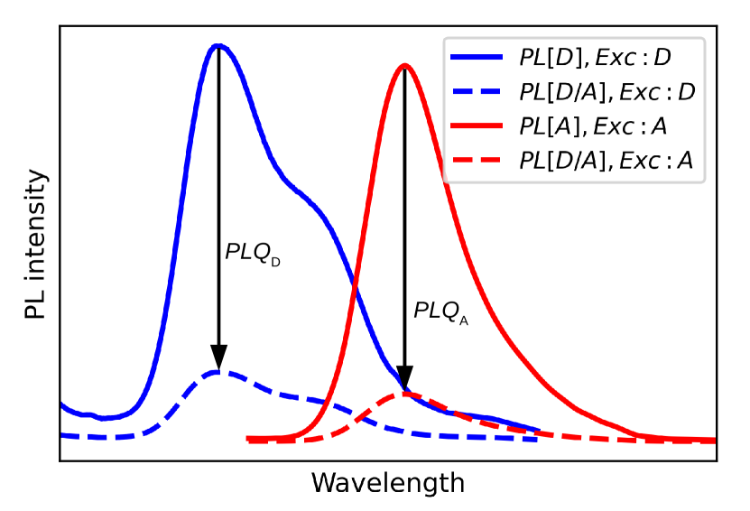
Over the years, the charge transfer (CT) process between electron donor (D) and electron acceptor (A) materials has been widely studied by photoluminescence (PL) measurements [1, 2, 3]. The PL effect corresponds to the light emission from the radiative exciton recombination after photon absorption in the material. Depending on the material combination, PL can be quenched due to interfacial charge transfer processes [3, 4]. One of the simplest ways to study this effect is by comparing the integrated PL intensity of pristine donor (PLD) with the corresponding quantity for the donoracceptor blend (PLDA) [5, 6]. In order to efficiently excite the singlet excitons in the donor, an excitation wavelength close to the main absorption band of the donor must be chosen. In order to selectively study the DA charge transfer, it is important to minimize the overlap between the donor and acceptor absorption spectrum [7]. This condition ensures that the majority of the excitons generated after photon absorption are created in the donor phase of the DA blend. The PL quenching efficiency of the donor excitonic luminescence () is then
| (1) |
If the excitation wavelength corresponds to acceptor’s main absorption band [8, 9], the quenching efficiency of the A phase () is quantified by comparing the PL of pristine acceptor () with
| (2) |
Figure 1 illustrates PL measurements using a fluorimeter after selective excitation of the donor or acceptor. The magnitudes of , and must be obtained by integrating over the entire measured spectrum. and are determined by the contributions of exciton dissociation or nonradiative (NR) exciton recombination at the DA interface. Both processes are intermediated by the creation of a charge transfer (CT) state formed after the electron transfer from the D to A or the hole transfer from A to D. For the measurement to capture these effects well, the majority of the generated excitons must reach the DA interface. In bulk heterojunction systems where the D and A materials are mixed, achieving this goal is relatively straightforward. It is essential to control the size of the materials domains to ensure that a significant proportion of excitons encounter the DA interface. In this context, the domain size should be roughly equivalent to the exciton diffusion length. Conversely, in bilayer heterojunctions, where the donor and acceptor are in separate layers, ensuring that most excitons reach the DA interface requires careful consideration of layer thickness. To maximize the chances of excitons reaching the DA interface, the thickness of the layers should be on the order of the exciton diffusion length. In summary, domain size control is pivotal in bulk heterojunctions, while layer thickness control plays a crucial role in bilayer heterojunctions. These considerations are fundamental to understand and optimize PLQ measurements.
The measurement of is a powerful tool to investigate photoluminescence quenching in DA blends. However, the application of this experimental method does not allow to study the details of the processes that contribute to the quenching. Deeper knowledge of the excited state dynamics at DA interfaces by kinetic modeling is fundamental to tailor the properties of the blend aiming at different applications [10, 11, 12, 13, 14, 15]. For example, for organic solar cells, exciton dissociation must be maximized and exciton recombination minimized to improve the efficiency of the photovoltaic process. On the other hand, for photothermal therapy, the maximization of NR exciton recombination is desirable to improve the heat generation produced after photon absorption [16]. Therefore, it is important to adopt a general approach that combines the analysis of the experimental data with simulations of and obtained from a kinetic model of exciton dissociation at the DA interface. The use of this method might reveal the full dynamics of excited states in DA blends which is fundamental to improving the performance of these materials towards a specific use.
Our group developed a theory to calculate and based on a kinetic model that considers all possible processes involved in exciton dynamics at the D/A interface [17, 18, 19]. We believe this model can be helpful for research groups interested in the dynamics of charge generation or exciton recombination induced by light excitation of DA blends. To provide broad access to this capability, we developed a freelicense and easy to handle software, Photoluminescence Quenching Simulator (PLQ-Sim). We also extend the original model to consider the time evolution of state populations following a similar procedure recently presented in ref. [15]. To perform a simulation, basic information about the materials forming the system (such as energy levels, dielectric constant, reorganization energy, and singlet exciton lifetime, for instance) must be provided as input parameters. If some information is missing, default values for the class of material studied can be used. After running the simulation, the rates of the physical processes involved in the charge dynamics at the DA interface (like the charge transfer or charge recombination rates, for instance) are provided as output. This information is crucial to characterize the photophysical process as a whole and to propose ideas for system optimizations. Therefore, our program aims to help the experimentalist to finetune fabrication process to maximize the PL quenching. PLQSim is a free license program compatible with Windows, Unix, and macOS operating systems developed in Python programming language.
2 Theoretical Methods
2.1 Kinetics of photoluminescence quenching
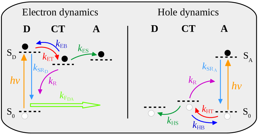
The model describes, using a simple oneelectron picture, the electron and hole kinetics at the DA interface. In addition to charge transfer, it also takes into account Fluorescence (or Förster) resonance energy transfer (FRET) [7, 20]. After donor excitation, four processes might occur with their corresponding characteristic rates: electron transfer (), singlet exciton recombination (), donordonorFRET () or donoracceptorFRET (). If electron transfer takes place, a charge transfer state (CT) is formed. From this intermediary excitation, three new kinetic steps might follow: electron separation (), electron return to regenerate the initial singlet state () or decay to the ground state by charge recombination from CT (). If instead of electron transfer the donoracceptorFRET takes place as a first step, the dynamics of the hole needs to be taken into account with analogous processes as those described above for electrons. The presence of donoracceptorFRET thus links the with the hole kinetics at the acceptor. Based on Ref. [21], Figure 2 illustrates the charge and energy transfer dynamics that will be studied here. The main objective of our model is to quantify the steady state values of and using the transfer rates of the characteristic processes as input parameters.
We start the description of the model assuming that there is on averaged excited donor molecules near an acceptor. In an interval , of those donors can transfer an electron to the acceptor to form a CT state (group 1). Alternatively, besides the electron transfer, of those donors have the additional possibility of performing an energy transfer by FRET to a nearby acceptor (group 2). From the above assumptions . Thus, for group 1 molecules, the time derivative of singlet exciton concentration, , is
| (3) |
where, is the concentration of CT states and is the exciton generation rate in the donor at the DA interface. This rate involves the excitons produced by direct photon absorption or resulting from the net flux of excitations transferred by FRET from (to) other donors. Using the above assumptions, time evolution of singlet state concentration for the group 2 of donors is given by
| (4) |
where the term was added to Eq. (3) from Eq. (4). By combining these equations one gets the total time variation of the singlet state concentration in the molecules
| (5) |
where . If is sufficiently high, the probability that one excited donor will belong to group 2 is . Hence Eq. (5) can be written as a function of
| (6) |
Upon charge transfer, the timedependent concentration of CT state at the DA heterojunction is related to by
| (7) |
In writing Eq. (7), we neglected the formation of CT states by direct absorption of light due to the low oscillation strength of this transition. Within the steady state approximation, Eq. (6) and Eq. (7) gives
| (8) |
| (9) |
| (10) |
where
| (11) |
After the DAFRET, the exciton at the acceptor can either recombine emitting a photon or be transferred to the CT state. Hence, the population of excitons in the acceptor also influences even for selective illumination of donor. Following the same reasoning used to derive Eq. (10), one can analogously write the population of (FRET induced) singlet excitons in the acceptor as
| (12) |
where
| (13) |
In Eq. (12), it is assumed that energy transfer from A to D is not allowed, so that .
In the absence of acceptors (hence assuming only donor molecules), the time derivative of singlet state concentration at the same position considered in Eq. (10) would give
| (14) |
where I’ is the rate of exciton generation in a donoronly material. Again assuming steady-state conditions, Eq. (14) gives,
| (15) |
or
| (16) |
Since the selective illumination of the donor can generate photoluminescence of the acceptor due to FRET, we define the donor’s PL quenching as
| (17) |
where we use Eq. (12). If the acceptor is inefficient to quench the excitons and , then from energy conservation. Eq. (17) then gives . Alternatively, if the acceptor is efficient to dissociate the excitons created in the donor, then and, from Eq. (17), . Note that the DAFRET is not dominant when so that the exciton quenching is determined mainly by electron transfer from the donor to the acceptor. On the other hand, if the exciton quenching will be determined by a sequential process that involves the DAFRET and the following transfer of holes to the donor. Using Eqs. (12) and (16), after some algebra, one gets
| (18) |
To completely assess the quenching dynamics described by Eq. (18), it is necessary to determine . We will assume that depends on the process that deactivates (or reactivates) the singlet donor state [22]. Under this assumption will be given by:
| (19) |
In the case of the formula for in Eq. (18) is reduced to the expression:
| (20) |
Finally, considering the selective excitation of the acceptor, we can repeat the same reasoning described above to calculate . Taking into account the absence of FRET from acceptor to the donor (), one can use a similar expression to Eq. (20) to write
| (21) |
See that from the kinetic model it is possible to obtain and using the transfer rates involved in the process.
2.2 Transfer rates calculation
The MarcusHush equation[23] is used in the program to calculate the characteristic frequencies involved in the charge transfer process
| (22) |
where , , , and are respectively the Boltzmann constant, temperature, reorganization energy, and electronic coupling (transfer integral). The activation energy for charge transfer, , is given by [24, 25]
| (23) |
where is the Gibbs free energy (driving force) of the charge transfer reaction, approximated here as the energy difference between final and initial states. As it will be demonstrated later, the reorganization energy, electronic coupling and energy levels are input parameters to the program. Specifically, the MarcusHush equation is used to obtain the frequency of the following rates: , , , , , and .
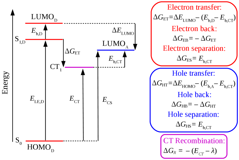
Figure 3 illustrates the energies involved in the kinetic processes depicted in Figure 1 as derived from the various energy levels of the system [26, 27]. The definitions of driving forces involved in the electron and hole dynamics at the DA interface are also shown in Figure 3. Note that, contrary to a common misconception that the driving force for electron () or hole transfer () is solely given by the energy offset between LUMOs () or HOMOs (), it also involves the binding energy of singlet ( and ) and CT states (). Only under the exceptional condition , the driving forces are simplified to and as assumed in several works. The for electron or hole back jump to recreate the singlet state is simply the negative of the respective transfer driving force. Considering the final step of exciton dissociation, the electron or hole separation, the driving force is given by the binding energy of the CT state. From the findings of Chen et al. [28], the for CT recombination () can be estimated as the negative of the CT state energy subtracted from the reorganization energy. When is estimated using this procedure, the found using the MarcusHush theory is similar to the rate derived using the MarcusLevichJortner model that considers the thermal population of high frequency vibrational modes [29].
The FRET rates between donors () and between donor and acceptor () are additional program inputs that must be provided by the user. Their quantification can be easily performed by a free program developed by our group called FRETCalc [7]. If FRET effects are negligible in the DA blend under study, the FRET rates can be set to zero in the input file. Additionally, if the user intends to study only , there is no need to provide the FRET rates. Finally, the singlet exciton recombination rate in each phase of the blend ( and ) is given by the inverse of the singlet exciton lifetime accessed from spectroscopy measurements in pristine materials, for instance.
2.3 Disorder effects
To better describe the charge transfer dynamics at the DA interface, the program also consider effects of diagonal disorder (energy levels fluctuations) and offdiagonal disorder (electronic coupling fluctuations between adjacent molecules due to random orientations) [23]. The diagonal disorder is considered by selecting a random value from a Gaussian distribution with mean zero and standard deviation (defined in the input) that is added to the driving forces.
For the calculations of offdiagonal effects, the user must define the maximum value for electronic coupling, , as an initial input. The program will then use the equation in the calculations to determine an specific value of the electronic coupling. The angle will be randomly chosen between and a userdefined maximum value () in the range . For example, if the user chooses , adjacent molecules will be considered randomly between the faceon configuration ( and ) and edgeon configuration ( and ).
When disorder is considered, the transfer rates, and become unique for each realization of parameters. It is then necessary to calculate average quantities to characterize the charge dynamics for a particular DA system. To obtain numerical averages with sufficient precision, it is recommended that the values of and are averaged over at least runs of parameters’ realization (defined in the input) of the simulation [12, 18]. Following this procedure, the average transfer rates, and are calculated.
2.4 Time evolution of state populations
The formalism described above was developed to quantify the photoluminescence quenching when the sample is submitted to a continuous excitation represented by the rate . However, in many situations a more complete characterization of the excited state dynamics can be obtained from timeresolved PL measurements. This motivated us to extend our model in order to broaden the applicability of the program.
Hence, besides the steady state PL quenching, the program can also calculate the time evolution of state population using the frequency rates specified above. In essence, this feature of our code can be applied to study experiments in which the sample is fully excited during a very short interval of time. The excited state decay kinetics is then obtained from the evolution of properties such as the intensity of emission response, for instance.
Modeling of this kind of experiment is done by generalizing the previous model to explicitly consider the evolution of molecule populations in the ground and charge separated states. This generalization is done by writing a set of coupled differential equations that describes the interdependent charge kinetics in the donor and in the acceptor. Basically these equations are derived from the general expression [30]
| (24) |
where is the state population at time . The appropriated solution of Eq. 24 is found by assuming that only singlet excited states are initially populated by a very short light pulse. Then, it follows that the decay obeys a multiexponential kinetics, with various effective rates. For a local acceptor excitation there are four coupled differential equations
| (25) |
where the initial condition is . Including the FRET process, six coupled differential equations are then needed to describe the kinetics derived from the donor local excitation
| (26) |
where the initial condition is . In Eq. (26), is the population of CT state generated from donor exciton, whereas is the population of CT state generated from acceptor exciton produced by FRET. The total population of CT state is given by, . The time interval considered for simulation is defined by the user in the program’s input file.
2.5 Limitations of the model
Although the model outlined above is efficient for simulating exciton dynamics at the DA interface, it has some limitations that are pointed out below. 1) The simulations implicitly assume that there are welldefined donor and acceptor domains and that all generated excitons reach the D/A interface. There is no need to define the heterojunction type before the simulation. Therefore, it is advisable to compare theoretical outcomes with experimental data wherein the predominant fraction of excitons does indeed reach the DA interface. 2) Photophysical processes occurring far from the DA interface region cannot be studied because the model only simulates the exciton dynamics in this region. 3) The model only considers singlet excitons, assuming that the dynamics of triplet excitons do not affect the PL quenching efficiency. It is meaningless to study with the model systems in which the flow of triplet excitons to the DA interface is relevant. 4) As the simulation approach is based on hopping model, whose intermolecular electronic coupling is much smaller than intramolecular charge reorganisation energy, tunneling effects that can assist the electron transfer are not considered. Therefore, systems with high electronic delocalization will not be well described by the model. In this way, we are assuming that the decoherence factor due to interaction with the vibrational degrees of freedom completely destroys the excitonic coherence, which leads to localization of the exciton. 5) The model was developed to simulate DA systems that are not exposed to an external electric field. Therefore, it is not possible to reproduce measurements under the influence of an external electric field.
2.6 Methods for obtaining input parameters
In this section we will briefly describe some popular methods found in the literature to obtain the input parameters necessary to run the PLQSim program. We emphasize that the methods presented below are just suggestions (it does not have the intention to be a complete summary of available experimentaltheoretical methods). Due to the extensive literature in the area, it is likely that there are other approach to obtain the same parameters.
2.6.1 Energy levels
The ionization potential (IP) and electron affinity (EA) are essential materials properties to calculate the driving forces for electron (hole) transfer. In principle, they can be determined by a combination of ultraviolet photoelectron spectroscopy (UPS) and inverse photoemission spectroscopy (IPES) [31]. Cyclic voltammetry (CV) is another alternative to access these parameters [32]. Following Koopmans’ theorem, the highest occupied molecular orbital (HOMO) energy can be considered as IP while the lowest unoccupied molecular orbital (LUMO) energy represents EA [33].
2.6.2 Energy of charge transfer state
2.6.3 Singlet exciton recombination lifetime
The singlet exciton recombination lifetime of pristine materials can be accessed using time-resolved photoluminescence (TRPL) spectroscopy [38].
2.6.4 Relative dielectric constant
The relative dielectric constant () of each material is also required as input. There are two common ways to obtain from experiments. The first is by performing capacitance measurements using impedance spectroscopy [39, 40]. is then calculated with the help of the equation [41], where is the capacitance, is the thickness of the film, is the permittivity of free space, and is the device area. The second technique involves the application of spectroscopic ellipsometry to find the real and imaginary components of the refractive index. In this case , where is measured in the longer wavelength limit to minimize absorption [42]. From density functional theory (DFT) calculations, the ClausiusMossotti equation can used to obtain [43, 44].
2.6.5 Reorganization energy
2.6.6 Electronic coupling
2.6.7 Exciton binding energy of pristine materials
The energy difference between the fundamental (or transport) band gap () and optical band gap () provides the exciton binding energy: . The fundamental band gap is the energy of free charge carriers (electron/hole): . The optical band gap is the energy of the lowest excited state of the semiconductor and can be extracted from the absorption onset in the UVvis spectrum [47].
DFT and timedependent DFT (TDDFT) calculations can also be used to obtain the gasphase exciton binding energy (). The first step is to apply DFT to obtain the groundstate geometry of isolated materials. Then, from single point calculations, the total energies of the cationic (), anionic (), and neutral () states can be determined. From these energies it is possible to calculate and . The optical gap can be obtained from TDDFT calculations and it corresponds to the energy of the lowest energy electronic transition excited by a single photon absorption. This procedure has been widely used in the literature [29, 44, 48, 49, 50]. The exciton binding energy in solidstate can be estimated by .
2.6.8 Exciton binding energy of charge transfer state
It is often assumed that the strong dielectric stabilization of the charge transfer (CT) state compensates the coulomb binding of a Frenkel exciton in the solid state, making [31]. We found in our previous work that there is a poor agreement between the simulated and measured using this approximation in the calculations [19]. There was a considerable improvement of the theoretical description if one slightly adjusts the in relation to . In fact, this is an interesting way to estimate the value of . Extensive research has been conducted to investigate the CT exciton binding energy in diverse DA blends through various techniques, revealing substantial variations [12, 51, 52].
2.7 Recommendations for users
We emphasize that due to the number of parameters involved in the model calculations, the theoretical estimates of and must always be confronted with experimental results. From this comparison, some input parameters, which may vary from material to material, can be finetuned to produce a better correlation between theory and experiment. Finally, we also emphasize that the theoretical model presented here has already been properly tested for several combinations of donor and acceptor materials showing good correlation with experiments and providing valuable insights about the physics behind exciton dissociation in systems under consideration [19, 16].
3 Software architecture, implementation and requirements
PLQSim is a free-license program. The binary files of this code (for Windows, Unix and macOS operational system) are available for download at PLQ-Sim repository on GitHub or can be run via dedicated webserver nanocalc.org. The program is implemented in Python 3 (v. 3.6)[53] and makes use of four Python libraries, namely Pandas [54], NumPy [55], and SciPy [56] for data manipulation and Matplotlib [57] for data visualization. The software was designed to be very userfriendly and take up little disk space, around 80 MB.
4 Program and Application
4.1 Input and basic demonstration
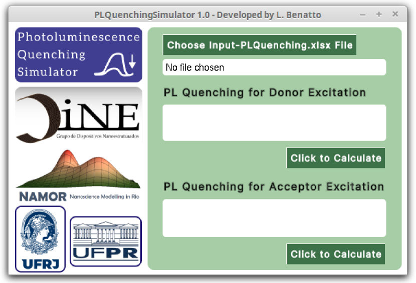
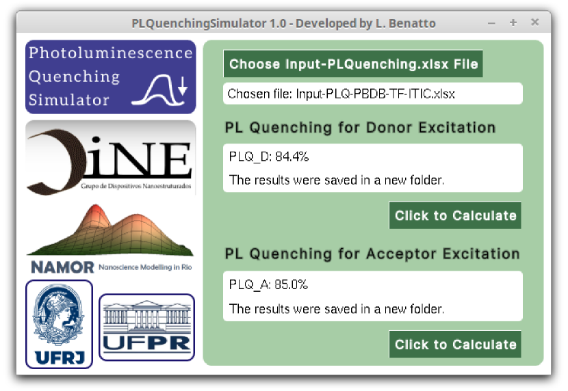
In this section, we will provide a practical example of how to perform a calculation using PLQSim. When the program starts, a graphical user interface is loaded. In order to utilize the interface, an input file must be provided as shown in Figure 4. The input file contains information on the system that will be simulated and must be in the xlsx (Excel file) format.
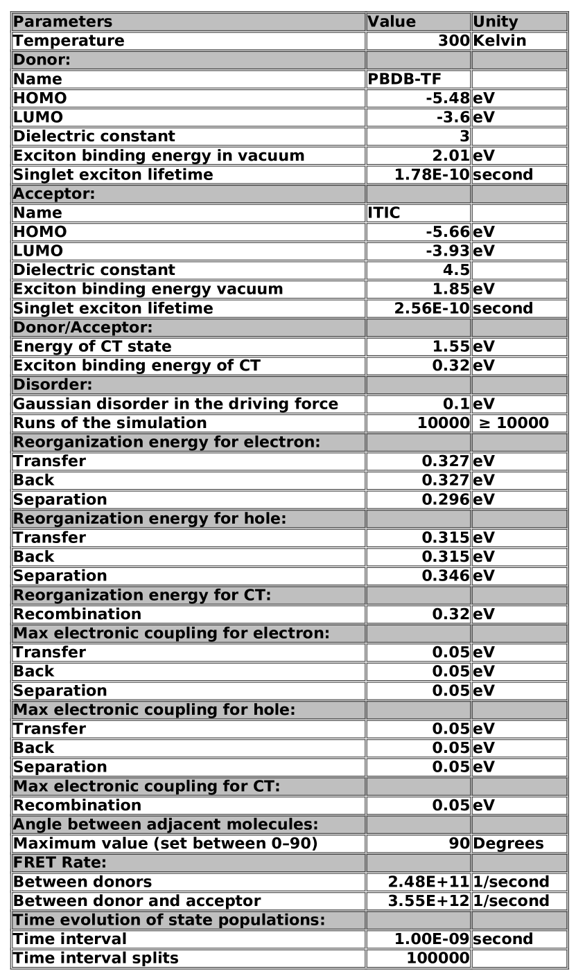
A modifiable input file will be included with the program as an illustrative example (see Figure 5). The default parameters utilized in this file were derived from literature and describe a DA blend of PBDBTF donor polymer [58] (also known as PM6 and PBDBT2F [59]) and the nonfullerene acceptor (NFA) ITIC molecule [60]. Those materials are current used in organic solar cells. The molecular energy levels of the materials considered here were obtained using CV measurements [32]. The singlet exciton recombination lifetimes of 178 ps for PBDBTF [31] and 256 ps for ITIC [38] were applied to find the singlet exciton recombination rates and . Dielectric constant, gasphase exciton binding energy, CT state energy and reorganization energy were obtained from Ref.[19]. For diagonal disorder, 0.1 eV was considered, which is a standard value for organic semiconductors [9, 61, 62]. The maximum value for electronic coupling was set to 50 meV for all processes, which is a typical value for the faceon configuration of adjacent molecules [62, 63, 64, 65]. The donoracceptor FRET rate were calculated using the FRETCalc software [7]. Another input information is . The specific value used in the input file was found by adjustment between theory and experiment. Finally, a total number of simulation runs was set as default in the input file. This number was found to give sufficiently accurate results (deviation in is less than 1% between simulations using the same set of input data). For the PBDBTFITIC blend, =82% and =85% were experimentally determined [32] while =84% and 85% were calculated using the PLQSim code (see Figure 6) with the set of parameters in Figure 5. As the theoretical and are consistent with the experiments, it is possible to use the additional software outputs to analyze the details of the charge dynamics on the DA interface.
4.2 Complementary outputs to PLQD and PLQA
Relevant data are printed in the Results_Donor.dat and Results_Acceptor.dat files. These data, such as transfer rates and quenching efficiency, are obtained by averaging over all specific information that are explicitly listed in the Results_Donor_Steps.dat and Results_Acceptor_Steps.dat files for each simulation step. In addition, two graphs that illustrate the electron (hole) dynamics at the DA interface (with the respective magnitudes of transfer rates) are automatically generated, see Figure 7.
The energy levels diagram and the schematic kinetics among excitons, CT states, and free charge carriers depicted in Figure 7 are very useful since it can provide the general scenario that determines the exciton dissociation or recombination. For example, in the Figure 7 (top), and have the same order of magnitude (1012 s-1) showing a clear competition between the electron transfer and the FRET phenomena to produce PL quenching. Furthermore, both rates are three orders of magnitude higher than 109 s-1, which is an important feature leading to enhancement. Another interesting result to be highlighted is that the electron separation rate 1010 s-1 is four orders of magnitude higher than the CT nonradiative recombination rate 106 s-1 and five orders of magnitude higher than the electron back rate to the singlet state 105 s-1. The magnitudes of these rates indicate that the donor excitation can create a significant density of CT and CS states at the DA interface.
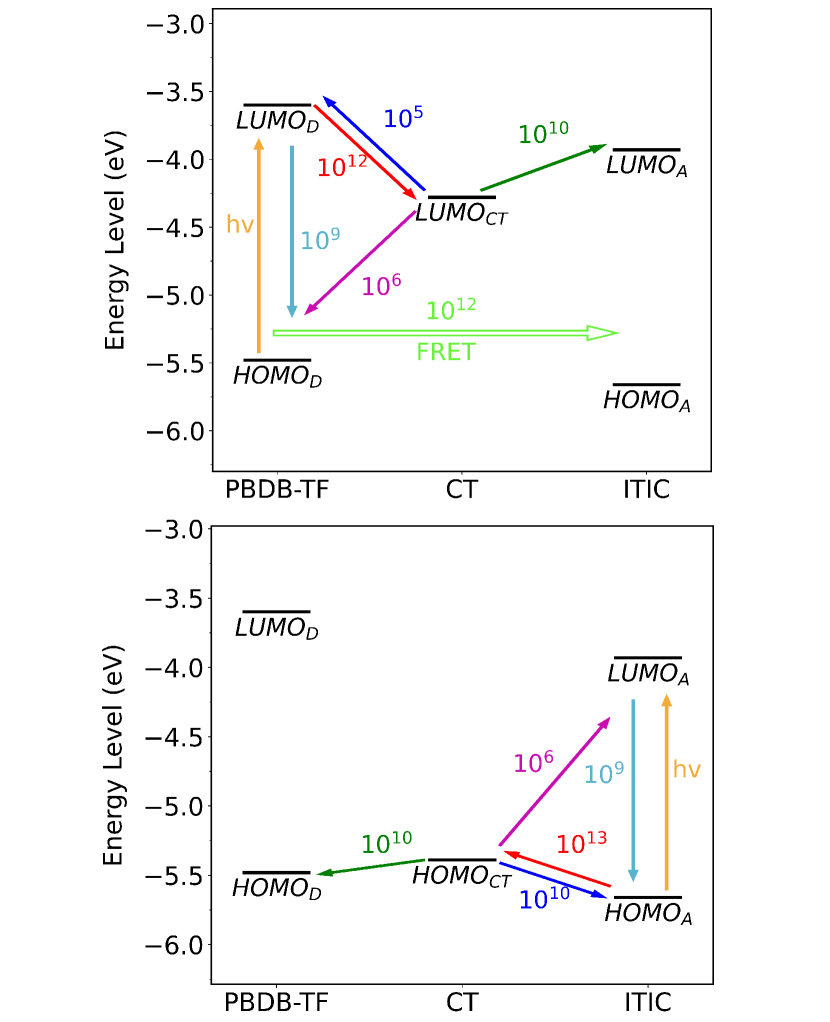
In addition, and in Figure 7 (bottom) have the same order of magnitude (1010 s-1), which suggests that there is a strong competition between the hole separation and back transfer processes. It is also possible to verify that 1013 s-1 is one order of magnitude greater than 1012 s-1. In other words, the DA interface is more efficient to transfer holes to the donor than electrons to the acceptor. Another important insight derived from Figure 7 is that the singlet recombination rate for acceptor excitons, 109 s-1, is three orders of magnitude greater than the nonradiative recombination rate of the CT state, 106 s-1. Since the hole transfer is very efficient, a low is essential to enhance the photovoltaic effect. On the other hand, considering the application of DA blends for photothermal conversion, faster exciton recombination and high heat generation might be found if [16].
4.3 Outputs for time evolution of state populations
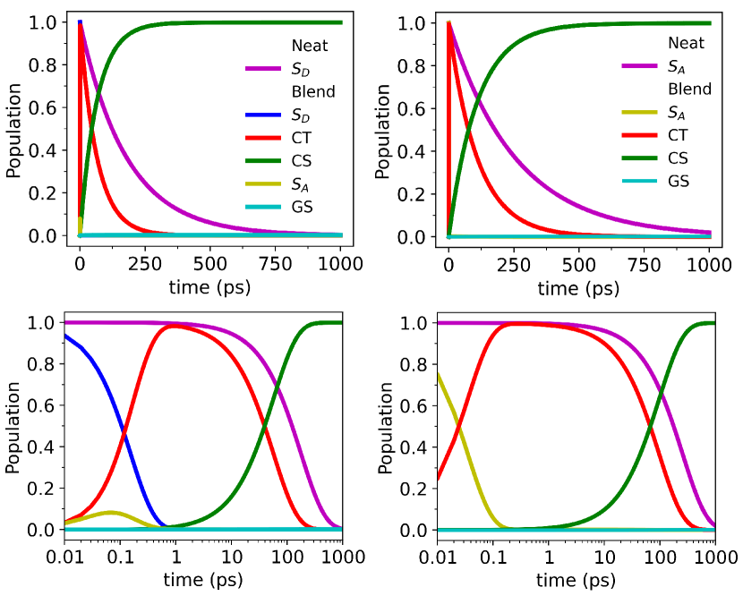
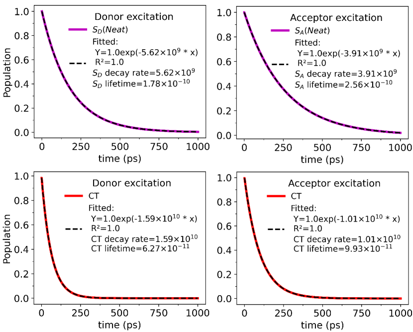
An additional output shows the time evolution of each state population. This tool is exemplified in Figure 8 for linear scale (top) and for logarithmic scale (bottom). Results on the left corresponds to donor excitation while those on the right to acceptor excitation. For comparison, we also calculate the population evolution of the single state that would be present in a pure donor or acceptor (i. e., disregarding the terms related to CT and CS in Eq. 25 and 26). The data showed in the Figure 8 are saved by the program in the files Time_Evolution_Donor.dat and Time_Evolution_Acceptor.dat. Note in Figure 8 that the blend population of and has a very sudden drop to zero (in less than 1 ps), a behavior that is in clear contrast to the kinetics observed for pure (neat) materials. This steep decay in the blend is due to the fast charge transfer rate ( and ) from the singlet state to form the CT state. In case of donor excitation, the high FRET rate induces the growth of the population which is rapidly extinguished by the fast hole transfer (). The population of the CT state is converted into the CS state over time because and are much faster than . As a consequence, the population of the GS state remains close to zero during the whole time interval analyzed since the majority of the excitons initially created are converted into free charges in this period. The simulated dynamics of the excited states are relevant to complement experimental studies of transient absorption (TA) on DA blends [11, 66].
A monoexponential fit of the time evolution displayed in Figure 8 enables the determination of an effective characteristic exciton lifetime and decay rate of the CT state. The program performs this analysis automatically and the results are shown in Figure 9. The exciton lifetime and decay rate for singlet states in the neat materials (SD(Neat) and SA(Neat)) are also calculated for comparison. As expected, the exciton lifetime of SD(A)(Neat) (top left and top right) is the same as the userdefined one set in the input file (obviously the decay rate is the inverse of this time). More interesting is the analysis of the CT state decay. It is described in the bottom left (right) of Figure 9 for donor (acceptor) excitation. Note that the decay rate of the CT state is close to the dissociation rate for the CS state, for donor (acceptor) excitation. Again, this feature of the blend originates from the slow CT decay () to ground state (GS). It is important to mention that the CT state lifetime calculated with the model implemented in the PLQSim code is consistent with recent experimental studies involving different polymerNFAs blends [67].
4.4 Exploring the software features
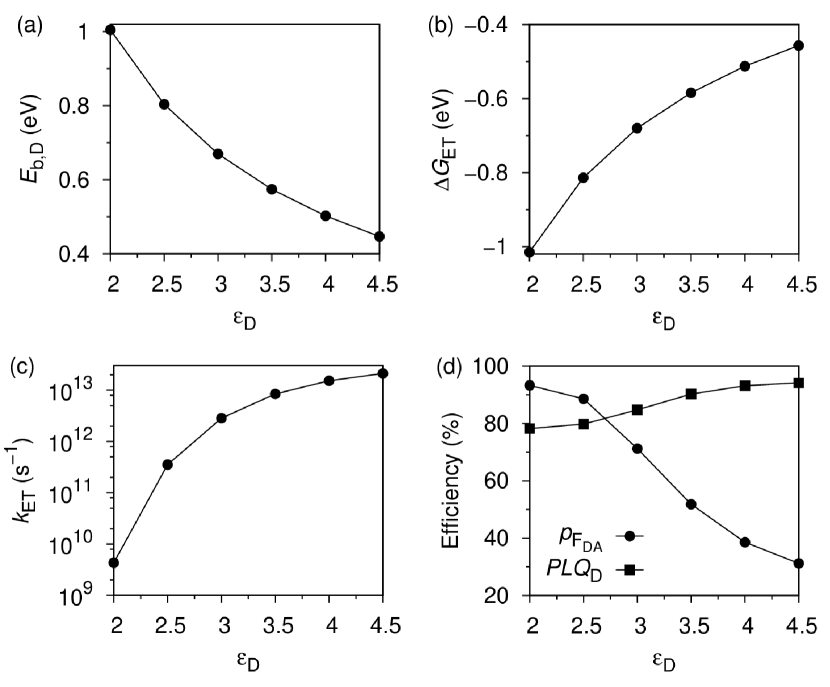
An interesting way to inspect the program is by varying the input parameters and checking their effect on the calculated quantities. Below we change some selected input parameters as examples of exploratory strategies to test the software’s capabilities. Let’s begin by varying the relative dielectric constant of donor (). One consequence of increasing is the reduction of the exciton binding energy, a feature that is evident in Figure 10a. The increase of also rises the driving force for electron transfer (, Figure 10b that can approach the reorganization energy for electron transfer. Here it is important to point out that the blend is in the Marcus inverted region (MIR) for electron transfer, characterized by in the framework of semiclassical Marcus theory. Therefore, the effect of decreases the activation energy for electron transfer which maximizes , as can be seen in Figure 10c. One can also observe in Figure 10d that the FRET probability from donor to acceptor is high in the interval where is low. As becomes higher, the FRET probability is greatly reduced, evidencing the negative correlation between charge transfer and energy transfer. Finally, higher values of in Figure 10d tend to maximize , mainly by the enhancing . Similar conclusions relative to the process of hole transfer and can be derived by considering variations of the acceptor relative dielectric constant ().
Discussion about the role played by disorder to determine some key properties of organic semiconductors has been the subject of a long debate in the literature [3, 23, 61, 68, 69, 70, 71]. The PLQSim code can help to answer these questions by opening the possibility to study, for instance, how depends on the disorder. This kind of analysis is exemplified in Figure 11a. It is clear that fluctuations in the driving forces associated to disorder tends to decrease .
The influence of the maximum angle between adjacent molecules () on is shown in Figure 11b. Note that is maximum for but slowly decreases until approximately . For higher angles, there is a more pronounced decrease until . Therefore, the increase in both kinds of disorder (diagonal, Figure 11a, and offdiagonal, Figure 11b) is detrimental to for the blend under consideration.
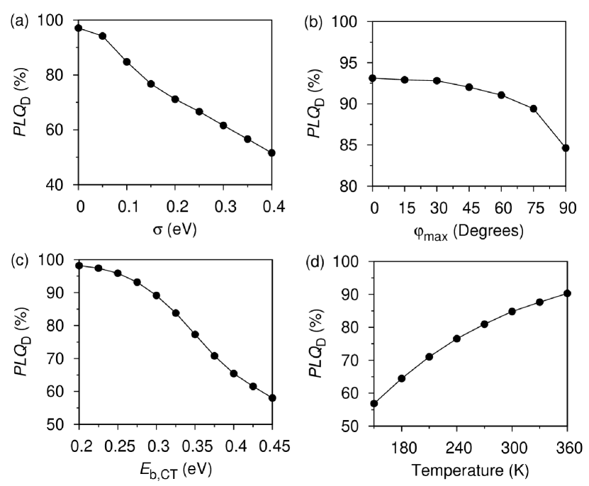
Another parameter that has a great impact on is the binding energy of the CT state. In Figure 11c one can see that the increase causes a regular drop of mainly originated by a continuous reduction. When becomes much smaller than the charge transfer rate (1012 s-1), exciton recombination is favored. Considering temperature effects in organic systems, there are reports in the literature of its beneficial impact on the exciton dissociation process [9, 71, 72]. In Figure 11d, indeed increases with temperature in agreement with the literature.
5 Conclusions
In summary, the theoretical background, a detailed demonstration, the applicability, and usefulness of the PLQSim program were described in detail. The program can be a powerful auxiliary tool to study the photoexcited state dynamics in DA blends through a userfriendly interface. In addition, the PLQSim program can be easily updated to implement new features suggested by the users due to its modular characteristics. We are confident that the various features offered by the PLQSim code will contribute significantly to the widespread adoption of this tool as a valuable instrument in researching more efficient organic devices based on DA blends.
Declaration of Competing Interest
The authors declare that they have no known competing financial interests or personal relationships that could have appeared to influence the work reported in this paper.
Acknowledgments
The authors acknowledge financial support from LCNano/SisNANO 2.0 (grant 442591/20195), INCT Carbon Nanomaterials, INCT Materials Informatics, and INCT NanoVIDA. L.B. (grant E26/202.091/2022 process 277806), O.M. (grant E26/200.729/2023 process 285493) and G.C. (grant E26/200.627/2022 and E26/210.391/2022 process 271814) are grateful for financial support from FAPERJ. The authors also acknowledge the computational support of Núcleo Avançado de Computação de Alto Desempenho (NACAD/COPPE/UFRJ), Sistema Nacional de Processamento de Alto Desempenho (SINAPAD), Centro Nacional de Processamento de Alto Desempenho em São Paulo (CENAPADSP), and technical support of SMMOLsolutions in functionalyzed materials.
6 Data availability
Data will be made available on request.
References
-
[1]
V. Arkhipov, H. Bässler, E. Emelyanova, D. Hertel, V. Gulbinas, L. Rothberg, Exciton dissociation in conjugated polymers, Macromol. Symp. 212 (1) (2004) 13–24.
doi:10.1002/masy.200450802.
URL https://onlinelibrary.wiley.com/doi/abs/10.1002/masy.200450802 -
[2]
V. I. Arkhipov, H. Bässler, M. Deussen, E. O. Göbel, R. Kersting, H. Kurz, U. Lemmer, R. F. Mahrt, Fieldinduced exciton breaking in conjugated polymers, Phys. Rev. B 52 (1995) 4932–4940.
doi:10.1103/PhysRevB.52.4932.
URL https://link.aps.org/doi/10.1103/PhysRevB.52.4932 -
[3]
G. Candiotto, A. Torres, K. T. Mazon, L. G. C. Rego, Charge generation in organic solar cells: Interplay of quantum dynamics, decoherence, and recombination, J. Phys. Chem. C 121 (42) (2017) 23276–23286.
doi:10.1021/acs.jpcc.7b07165.
URL https://doi.org/10.1021/acs.jpcc.7b07165 -
[4]
H. Ohkita, S. Cook, Y. Astuti, W. Duffy, S. Tierney, W. Zhang, M. Heeney, I. McCulloch, J. Nelson, D. D. C. Bradley, J. R. Durrant, Charge carrier formation in polythiophene/fullerene blend films studied by transient absorption spectroscopy, J. Am. Chem. Soc. 130 (10) (2008) 3030–3042.
doi:10.1021/ja076568q.
URL https://doi.org/10.1021/ja076568q -
[5]
M. Theander, A. Yartsev, D. Zigmantas, V. Sundström, W. Mammo, M. R. Andersson, O. Inganäs, Photoluminescence quenching at a heterojunction, Phys. Rev. B 61 (2000) 12957–12963.
doi:10.1103/PhysRevB.61.12957.
URL https://link.aps.org/doi/10.1103/PhysRevB.61.12957 -
[6]
K. Vandewal, Z. Ma, J. Bergqvist, Z. Tang, E. Wang, P. Henriksson, K. Tvingstedt, M. R. Andersson, F. Zhang, O. Inganäs, Quantification of quantum efficiency and energy losses in low bandgap polymer:fullerene solar cells with high open-circuit voltage, Adv. Funct. Mater. 22 (16) (2012) 3480–3490.
doi:10.1002/adfm.201200608.
URL https://onlinelibrary.wiley.com/doi/abs/10.1002/adfm.201200608 -
[7]
L. Benatto, O. Mesquita, J. L. Rosa, L. S. Roman, M. Koehler, R. B. Capaz, G. Candiotto, Fret–calc: A free software and web server for förster resonance energy transfer calculation, Comput. Phys. Commun. 287 (2023) 108715.
doi:10.1016/j.cpc.2023.108715.
URL https://www.sciencedirect.com/science/article/pii/S0010465523000607 -
[8]
H. Cha, S. Wheeler, S. Holliday, S. D. Dimitrov, A. Wadsworth, H. H. Lee, D. Baran, I. McCulloch, J. R. Durrant, Influence of blend morphology and energetics on charge separation and recombination dynamics in organic solar cells incorporating a nonfullerene acceptor, Adv. Funct. Mater. 28 (3) (2018) 1704389.
doi:10.1002/adfm.201704389.
URL https://onlinelibrary.wiley.com/doi/abs/10.1002/adfm.201704389 -
[9]
M. Gerhard, A. P. Arndt, I. A. Howard, A. RahimiIman, U. Lemmer, M. Koch, Temperature and energydependent separation of chargetransfer states in ptb7based organic solar cells, J. Phys. Chem. C 119 (51) (2015) 28309–28318.
doi:10.1021/acs.jpcc.5b09842.
URL https://doi.org/10.1021/acs.jpcc.5b09842 -
[10]
M. S. Vezie, M. Azzouzi, A. M. Telford, T. R. Hopper, A. B. Sieval, J. C. Hummelen, K. Fallon, H. Bronstein, T. Kirchartz, A. A. Bakulin, T. M. Clarke, J. Nelson, Impact of marginal exciton–charge-transfer state offset on charge generation and recombination in polymer:fullerene solar cells, ACS Energy Lett. 4 (9) (2019) 2096–2103.
doi:10.1021/acsenergylett.9b01368.
URL https://doi.org/10.1021/acsenergylett.9b01368 -
[11]
Y. Zhong, M. Causa’, G. J. Moore, P. Krauspe, B. Xiao, F. Günther, J. Kublitski, R. Shivhare, J. Benduhn, S. Mukherjee, et al., Subpicosecond chargetransfer at nearzero driving force in polymer: nonfullerene acceptor blends and bilayers, Nat. Commun. 11 (1) (2020) 833.
doi:10.1038/s41467-020-14549-w.
URL https://doi.org/10.1038/s41467-020-14549-w -
[12]
M. Gerhard, A. P. Arndt, M. Bilal, U. Lemmer, M. Koch, I. A. Howard, Field-induced exciton dissociation in ptb7-based organic solar cells, Phys. Rev. B 95 (2017) 195301.
doi:10.1103/PhysRevB.95.195301.
URL https://link.aps.org/doi/10.1103/PhysRevB.95.195301 -
[13]
O. J. Sandberg, A. Armin, Energetics and kinetics requirements for organic solar cells to break the 20% power conversion efficiency barrier, J. Phys. Chem. C 125 (28) (2021) 15590–15598.
doi:10.1021/acs.jpcc.1c03656.
URL https://doi.org/10.1021/acs.jpcc.1c03656 -
[14]
M. Azzouzi, N. P. Gallop, F. Eisner, J. Yan, X. Zheng, H. Cha, Q. He, Z. Fei, M. Heeney, A. A. Bakulin, et al., Reconciling models of interfacial state kinetics and device performance in organic solar cells: impact of the energy offsets on the power conversion efficiency, Energy Environ. Sci. 15 (3) (2022) 1256–1270.
doi:10.1039/D1EE02788C.
URL https://doi.org/10.1039/D1EE02788C -
[15]
A. Landi, D. Padula, Multiple charge separation pathways in new-generation non-fullerene acceptors: a computational study, J. Mater. Chem. A 9 (44) (2021) 24849–24856.
doi:10.1039/D1TA05664F.
URL https://doi.org/10.1039/D1TA05664F -
[16]
D. C. Grodniski, L. Benatto, J. P. Gonçalves, C. C. de Oliveira, K. R. M. Pacheco, L. B. Adad, V. M. Coturi, L. S. Roman, M. Koehler, High photothermal conversion efficiency for semiconducting polymer/fullerene nanoparticles and its correlation with photoluminescence quenching, Mater. Adv. 4 (2023) 486–503.
doi:10.1039/D2MA00912A.
URL http://dx.doi.org/10.1039/D2MA00912A -
[17]
L. Benatto, M. d. J. Bassi, L. C. W. de Menezes, L. S. Roman, M. Koehler, Kinetic model for photoluminescence quenching by selective excitation of d/a blends: implications for charge separation in fullerene and non-fullerene organic solar cells, J. Mater. Chem. C 8 (2020) 8755–8769.
doi:10.1039/D0TC01077D.
URL http://dx.doi.org/10.1039/D0TC01077D -
[18]
L. Benatto, C. A. M. Moraes, M. de Jesus Bassi, L. Wouk, L. S. Roman, M. Koehler, Kinetic modeling of the electric field dependent exciton quenching at the donor–acceptor interface, J. Phys. Chem. C 125 (8) (2021) 4436–4448.
doi:10.1021/acs.jpcc.0c11458.
URL https://doi.org/10.1021/acs.jpcc.0c11458 -
[19]
L. Benatto, C. A. M. Moraes, G. Candiotto, K. R. A. Sousa, J. P. A. Souza, L. S. Roman, M. Koehler, Conditions for efficient charge generation preceded by energy transfer process in non-fullerene organic solar cells, J. Mater. Chem. A 9 (2021) 27568–27585.
doi:10.1039/D1TA06698F.
URL http://dx.doi.org/10.1039/D1TA06698F -
[20]
G. Candiotto, R. Giro, B. A. C. Horta, F. P. Rosselli, M. de Cicco, C. A. Achete, M. Cremona, R. B. Capaz, Emission redshift in dcm2-doped caused by nonlinear stark shifts and förster-mediated exciton diffusion, Phys. Rev. B 102 (2020) 235401.
doi:10.1103/PhysRevB.102.235401.
URL https://link.aps.org/doi/10.1103/PhysRevB.102.235401 -
[21]
X.-Y. Zhu, How to draw energy level diagrams in excitonic solar cells, J. Phys. Chem. Lett. 5 (13) (2014) 2283–2288.
doi:10.1021/jz5008438.
URL https://doi.org/10.1021/jz5008438 -
[22]
K. F. Chou, A. M. Dennis, Förster resonance energy transfer between quantum dot donors and quantum dot acceptors, Sensors 15 (6) (2015) 13288–13325.
doi:10.3390/s150613288.
URL https://www.mdpi.com/1424-8220/15/6/13288 -
[23]
V. Coropceanu, J. Cornil, D. A. da Silva Filho, Y. Olivier, R. Silbey, J.-L. Brédas, Charge transport in organic semiconductors, Chem. Rev. 107 (4) (2007) 926–952.
doi:10.1021/cr050140x.
URL https://doi.org/10.1021/cr050140x -
[24]
H. Oberhofer, K. Reuter, J. Blumberger, Charge transport in molecular materials: An assessment of computational methods, Chem. Rev. 117 (15) (2017) 10319–10357.
doi:10.1021/acs.chemrev.7b00086.
URL https://doi.org/10.1021/acs.chemrev.7b00086 -
[25]
L. Merces, G. Candiotto, L. M. M. Ferro, A. de Barros, C. V. S. Batista, A. Nawaz, A. Riul Jr., R. B. Capaz, C. C. B. Bufon, Reorganization energy upon controlled intermolecular charge-transfer reactions in monolithically integrated nanodevices, Small 17 (45) (2021) 2103897.
doi:10.1002/smll.202103897.
URL https://onlinelibrary.wiley.com/doi/abs/10.1002/smll.202103897 -
[26]
K. Nakano, Y. Chen, B. Xiao, W. Han, J. Huang, H. Yoshida, E. Zhou, K. Tajima, Anatomy of the energetic driving force for charge generation in organic solar cells, Nat. Commun. 10 (1) (2019) 2520.
doi:10.1038/s41467-019-10434-3.
URL https://doi.org/10.1038/s41467-019-10434-3 -
[27]
D. Qian, Z. Zheng, H. Yao, W. Tress, T. R. Hopper, S. Chen, S. Li, J. Liu, S. Chen, J. Zhang, et al., Design rules for minimizing voltage losses in high-efficiency organic solar cells, Nat. Mater. 17 (8) (2018) 703–709.
doi:10.1038/s41563-018-0128-z.
URL https://doi.org/10.1038/s41563-018-0128-z -
[28]
X.-K. Chen, M. K. Ravva, H. Li, S. M. Ryno, J.-L. Brédas, Effect of molecular packing and charge delocalization on the nonradiative recombination of charge-transfer states in organic solar cells, Adv. Energy Mater. 6 (24) (2016) 1601325.
doi:10.1002/aenm.201601325.
URL https://onlinelibrary.wiley.com/doi/abs/10.1002/aenm.201601325 -
[29]
L. Benatto, M. Koehler, Effects of fluorination on exciton binding energy and charge transport of -conjugated donor polymers and the itic molecular acceptor: A theoretical study, J. Phys. Chem. C 123 (11) (2019) 6395–6406.
doi:10.1021/acs.jpcc.8b12261.
URL https://doi.org/10.1021/acs.jpcc.8b12261 -
[30]
L. Cupellini, S. Giannini, B. Mennucci, Electron and excitation energy transfers in covalently linked donor–acceptor dyads: mechanisms and dynamics revealed using quantum chemistry, Phys. Chem. Chem. Phys. 20 (2018) 395–403.
doi:10.1039/C7CP07002K.
URL http://dx.doi.org/10.1039/C7CP07002K -
[31]
S. Karuthedath, J. Gorenflot, Y. Firdaus, N. Chaturvedi, C. S. De Castro, G. T. Harrison, J. I. Khan, A. Markina, A. H. Balawi, T. A. D. Peña, et al., Intrinsic efficiency limits in low-bandgap non-fullerene acceptor organic solar cells, Nat. Mater. 20 (3) (2021) 378–384.
doi:10.1038/s41563-020-00835-x.
URL https://doi.org/10.1038/s41563-020-00835-x -
[32]
C. Yang, J. Zhang, N. Liang, H. Yao, Z. Wei, C. He, X. Yuan, J. Hou, Effects of energy-level offset between a donor and acceptor on the photovoltaic performance of non-fullerene organic solar cells, J. Mater. Chem. A 7 (2019) 18889–18897.
doi:10.1039/C9TA04789A.
URL http://dx.doi.org/10.1039/C9TA04789A -
[33]
J.-L. Bredas, Mind the gap!, Mater. Horiz. 1 (2014) 17–19.
doi:10.1039/C3MH00098B.
URL http://dx.doi.org/10.1039/C3MH00098B -
[34]
M. List, T. Sarkar, P. Perkhun, J. Ackermann, C. Luo, U. Würfel, Correct determination of charge transfer state energy from luminescence spectra in organic solar cells, Nat. Commun. 9 (1) (2018) 3631.
doi:10.1038/s41467-018-05987-8.
URL https://doi.org/10.1038/s41467-018-05987-8 -
[35]
L. C. Wouk de Menezes, Y. Jin, L. Benatto, C. Wang, M. Koehler, F. Zhang, L. S. Roman, Charge transfer dynamics and device performance of environmentally friendly processed nonfullerene organic solar cells, ACS Appl. Energy Mater. 1 (9) (2018) 4776–4785.
doi:10.1021/acsaem.8b00884.
URL https://doi.org/10.1021/acsaem.8b00884 -
[36]
H. Zong, X. Wang, J. Quan, C. Tian, M. Sun, Photoinduced charge transfer by one and two-photon absorptions: physical mechanisms and applications, Phys. Chem. Chem. Phys. 20 (2018) 19720–19743.
doi:10.1039/C8CP03442G.
URL http://dx.doi.org/10.1039/C8CP03442G -
[37]
Q. Wang, Y. Li, P. Song, R. Su, F. Ma, Y. Yang, Nonfullerene acceptor-based solar cells: From structural design to interface charge separation and charge transport, Polymers 9 (12) (2017).
doi:10.3390/polym9120692.
URL https://www.mdpi.com/2073-4360/9/12/692 -
[38]
F. Yang, D. Qian, A. H. Balawi, Y. Wu, W. Ma, F. Laquai, Z. Tang, F. Zhang, W. Li, Performance limitations in thieno[3,4-c]pyrrole-4,6-dione-based polymer:itic solar cells, Phys. Chem. Chem. Phys. 19 (2017) 23990–23998.
doi:10.1039/C7CP04780K.
URL http://dx.doi.org/10.1039/C7CP04780K -
[39]
T. Li, K. Wang, G. Cai, Y. Li, H. Liu, Y. Jia, Z. Zhang, X. Lu, Y. Yang, Y. Lin, Asymmetric glycolated substitution for enhanced permittivity and ecocompatibility of high-performance photovoltaic electron acceptor, JACS Au 1 (10) (2021) 1733–1742.
doi:10.1021/jacsau.1c00306.
URL https://doi.org/10.1021/jacsau.1c00306 -
[40]
X. Zhang, D. Zhang, Q. Zhou, R. Wang, J. Zhou, J. Wang, H. Zhou, Y. Zhang, Fluorination with an enlarged dielectric constant prompts charge separation and reduces bimolecular recombination in nonfullerene organic solar cells with a high fill factor and efficiency ¿13%, Nano Energy 56 (2019) 494–501.
doi:10.1016/j.nanoen.2018.11.067.
URL https://www.sciencedirect.com/science/article/pii/S2211285518308796 -
[41]
X. Liu, B. Xie, C. Duan, Z. Wang, B. Fan, K. Zhang, B. Lin, F. J. M. Colberts, W. Ma, R. A. J. Janssen, F. Huang, Y. Cao, A high dielectric constant nonfullerene acceptor for efficient bulkheterojunction organic solar cells, J. Mater. Chem. A 6 (2018) 395–403.
doi:10.1039/C7TA10136H.
URL http://dx.doi.org/10.1039/C7TA10136H -
[42]
H. T. Chandran, T.-W. Ng, Y. Foo, H.-W. Li, J. Qing, X.-K. Liu, C.-Y. Chan, F.-L. Wong, J. A. Zapien, S.-W. Tsang, M.-F. Lo, C.-S. Lee, Direct free carrier photogeneration in single layer and stacked organic photovoltaic devices, Adv. Mater. 29 (22) (2017) 1606909.
doi:10.1002/adma.201606909.
URL https://onlinelibrary.wiley.com/doi/abs/10.1002/adma.201606909 -
[43]
P. Schwenn, P. Burn, B. Powell, Calculation of solid state molecular ionisation energies and electron affinities for organic semiconductors, Org. Electron. 12 (2) (2011) 394–403.
doi:10.1016/j.orgel.2010.11.025.
URL https://www.sciencedirect.com/science/article/pii/S1566119910003836 -
[44]
L. Benatto, C. F. N. Marchiori, C. M. Araujo, M. Koehler, Molecular origin of efficient hole transfer from nonfullerene acceptors: insights from firstprinciples calculations, J. Mater. Chem. C 7 (2019) 12180–12193.
doi:10.1039/C9TC03563J.
URL http://dx.doi.org/10.1039/C9TC03563J -
[45]
G. R. Hutchison, M. A. Ratner, T. J. Marks, Hopping transport in conductive heterocyclic oligomers: reorganization energies and substituent effects, J. Am. Chem. Soc. 127 (7) (2005) 2339–2350.
doi:10.1021/ja0461421.
URL https://doi.org/10.1021/ja0461421 -
[46]
S. Gorelsky, A. Lever, Electronic structure and spectra of ruthenium diimine complexes by density functional theory and indo/s. comparison of the two methods, J. Organomet. Chem. 635 (1) (2001) 187–196.
doi:10.1016/S0022-328X(01)01079-8.
URL https://www.sciencedirect.com/science/article/pii/S0022328X01010798 -
[47]
J. Zhang, J. Guan, Y. Zhang, S. Qin, Q. Zhu, X. Kong, Q. Ma, X. Li, L. Meng, Y. Yi, J. Zheng, Y. Li, Direct observation of increased free carrier generation owing to reduced exciton binding energies in polymerized small-molecule acceptors, J. Phys. Chem. Lett 13 (38) (2022) 8816–8824.
doi:10.1021/acs.jpclett.2c02337.
URL https://doi.org/10.1021/acs.jpclett.2c02337 -
[48]
L. Zhu, Y. Yi, Z. Wei, Exciton binding energies of nonfullerene small molecule acceptors: Implication for exciton dissociation driving forces in organic solar cells, J. Phys. Chem. C 122 (39) (2018) 22309–22316.
doi:10.1021/acs.jpcc.8b07197.
URL https://doi.org/10.1021/acs.jpcc.8b07197 -
[49]
J.-C. Lee, J.-D. Chai, S.-T. Lin, Assessment of density functional methods for exciton binding energies and related optoelectronic properties, RSC Adv. 5 (2015) 101370–101376.
doi:10.1039/C5RA20085G.
URL http://dx.doi.org/10.1039/C5RA20085G -
[50]
L. Benatto, J. P. A. Souza, M. F. F. das Neves, L. S. Roman, R. B. Capaz, G. Candiotto, M. Koehler, Enhancing the chemical stability and photovoltaic properties of highly efficient nonfullerene acceptors by chalcogen substitution: Insights from quantum chemical calculations, ACS Appl. Energy Mater 0 (0) (2023) null.
doi:10.1021/acsaem.3c02371.
URL https://doi.org/10.1021/acsaem.3c02371 -
[51]
S. Athanasopoulos, F. Schauer, V. Nádaždy, M. Weiß, F.-J. Kahle, U. Scherf, H. Bässler, A. Köhler, What is the binding energy of a charge transfer state in an organic solar cell?, Adv. Energy Mater. 9 (24) (2019) 1900814.
doi:https://doi.org/10.1002/aenm.201900814.
URL https://onlinelibrary.wiley.com/doi/abs/10.1002/aenm.201900814 -
[52]
Y. Dong, H. Cha, J. Zhang, E. Pastor, P. S. Tuladhar, I. McCulloch, J. R. Durrant, A. A. Bakulin, The binding energy and dynamics of charge-transfer states in organic photovoltaics with low driving force for charge separation, J. Chem. Phys. 150 (10) (2019) 104704.
doi:10.1063/1.5079285.
URL https://doi.org/10.1063/1.5079285 -
[53]
G. Van Rossum, F. L. Drake, Python 3 Reference Manual, CreateSpace, Scotts Valley, CA, 2009.
doi:10.5555/1593511.
URL https://dl.acm.org/doi/book/10.5555/1593511 -
[54]
W. McKinney, Data Structures for statistical computing in python, in: Proceedings of the 9th Python in Science Conference, Vol. 445, 2010, pp. 56–61.
doi:10.25080/Majora-92bf1922-00a.
URL https://conference.scipy.org/proceedings/scipy2010/mckinney.html -
[55]
C. R. Harris, K. J. Millman, S. J. Van Der Walt, R. Gommers, P. Virtanen, D. Cournapeau, E. Wieser, J. Taylor, S. Berg, N. J. Smith, et al., Array programming with numpy, Nature 585 (7825) (2020) 357–362.
doi:doi.org/10.1038/s41586-020-2649-2.
URL https://www.nature.com/articles/s41586-020-2649-2 -
[56]
P. Virtanen, R. Gommers, T. E. Oliphant, M. Haberland, T. Reddy, D. Cournapeau, E. Burovski, P. Peterson, W. Weckesser, J. Bright, et al., Scipy 1.0: fundamental algorithms for scientific computing in python, Nat. Methods 17 (3) (2020) 261–272.
doi:doi.org/10.1038/s41592-019-0686-2.
URL https://www.nature.com/articles/s41592-019-0686-2 -
[57]
J. D. Hunter, Matplotlib: A 2d graphics environment, Comput. Sci. Eng. 9 (03) (2007) 90–95.
doi:doi.org/10.1109/MCSE.2007.55.
URL https://www.computer.org/csdl/magazine/cs/2007/03/c3090/13rRUwbJD0A -
[58]
M. Zhang, X. Guo, W. Ma, H. Ade, J. Hou, A largebandgap conjugated polymer for versatile photovoltaic applications with high performance, Adv. Mater. 27 (31) (2015) 4655–4660.
doi:https://doi.org/10.1002/adma.201502110.
URL https://onlinelibrary.wiley.com/doi/abs/10.1002/adma.201502110 -
[59]
Z. Zheng, H. Yao, L. Ye, Y. Xu, S. Zhang, J. Hou, Pbdbt and its derivatives: A family of polymer donors enables over 17% efficiency in organic photovoltaics, Mater. Today 35 (2020) 115–130.
doi:https://doi.org/10.1016/j.mattod.2019.10.023.
URL https://www.sciencedirect.com/science/article/pii/S1369702119308363 -
[60]
W. Zhao, D. Qian, S. Zhang, S. Li, O. Inganäs, F. Gao, J. Hou, Fullerene-free polymer solar cells with over 11% efficiency and excellent thermal stability, Adv. Mater. 28 (23) (2016) 4734–4739.
doi:https://doi.org/10.1002/adma.201600281.
URL https://onlinelibrary.wiley.com/doi/abs/10.1002/adma.201600281 -
[61]
O. Rubel, S. D. Baranovskii, W. Stolz, F. Gebhard, Exact solution for hopping dissociation of geminate electron-hole pairs in a disordered chain, Phys. Rev. Lett. 100 (2008) 196602.
doi:10.1103/PhysRevLett.100.196602.
URL https://link.aps.org/doi/10.1103/PhysRevLett.100.196602 -
[62]
X.-K. Chen, D. Qian, Y. Wang, T. Kirchartz, W. Tress, H. Yao, J. Yuan, M. Hülsbeck, M. Zhang, Y. Zou, et al., A unified description of non-radiative voltage losses in organic solar cells, Nat. Energy 6 (8) (2021) 799–806.
doi:10.1038/s41560-021-00843-4.
URL https://doi.org/10.1038/s41560-021-00843-4 -
[63]
K. Do, Q. Saleem, M. K. Ravva, F. Cruciani, Z. Kan, J. Wolf, M. R. Hansen, P. M. Beaujuge, J.-L. Brédas, Impact of fluorine substituents on -conjugated polymer main-chain conformations, packing, and electronic couplings, Adv. Mat. 28 (37) (2016) 8197–8205.
doi:https://doi.org/10.1002/adma.201601282.
URL https://onlinelibrary.wiley.com/doi/abs/10.1002/adma.201601282 -
[64]
T. J. Aldrich, M. Matta, W. Zhu, S. M. Swick, C. L. Stern, G. C. Schatz, A. Facchetti, F. S. Melkonyan, T. J. Marks, Fluorination effects on indacenodithienothiophene acceptor packing and electronic structure, end-group redistribution, and solar cell photovoltaic response, J. Am. Chem. Soc. 141 (7) (2019) 3274–3287.
doi:10.1021/jacs.8b13653.
URL https://doi.org/10.1021/jacs.8b13653 -
[65]
Y. Firdaus, V. M. Le Corre, S. Karuthedath, W. Liu, A. Markina, W. Huang, S. Chattopadhyay, M. M. Nahid, M. I. Nugraha, Y. Lin, et al., Long-range exciton diffusion in molecular non-fullerene acceptors, Nat. Commun. 11 (1) (2020) 5220.
doi:10.1038/s41467-020-19029-9.
URL https://doi.org/10.1038/s41467-020-19029-9 -
[66]
A. Classen, C. L. Chochos, L. Lüer, V. G. Gregoriou, J. Wortmann, A. Osvet, K. Forberich, I. McCulloch, T. Heumüller, C. J. Brabec, The role of exciton lifetime for charge generation in organic solar cells at negligible energy-level offsets, Nat. Energy 5 (9) (2020) 711–719.
doi:10.1038/s41560-020-00684-7.
URL https://doi.org/10.1038/s41560-020-00684-7 -
[67]
Y. Dong, H. Cha, H. L. Bristow, J. Lee, A. Kumar, P. S. Tuladhar, I. McCulloch, A. A. Bakulin, J. R. Durrant, Correlating charge-transfer state lifetimes with material energetics in polymer:non-fullerene acceptor organic solar cells, J. Am. Chem. Soc. 143 (20) (2021) 7599–7603.
doi:10.1021/jacs.1c00584.
URL https://doi.org/10.1021/jacs.1c00584 -
[68]
P. Peumans, S. R. Forrest, Separation of geminate charge-pairs at donor–acceptor interfaces in disordered solids, Chem. Phys. Lett. 398 (1) (2004) 27–31.
doi:10.1016/j.cplett.2004.09.030.
URL https://www.sciencedirect.com/science/article/pii/S0009261404014186 -
[69]
M. Koehler, M. C. Santos, M. G. E. da Luz, Positional disorder enhancement of exciton dissociation at donoracceptor interface, J. Appl. Phys. 99 (5) (2006) 053702.
doi:10.1063/1.2174118.
URL https://doi.org/10.1063/1.2174118 -
[70]
S. Liu, J. Yuan, W. Deng, M. Luo, Y. Xie, Q. Liang, Y. Zou, Z. He, H. Wu, Y. Cao, High-efficiency organic solar cells with low non-radiative recombination loss and low energetic disorder, Nat. Photonics 14 (5) (2020) 300–305.
doi:10.1038/s41566-019-0573-5.
URL https://doi.org/10.1038/s41566-019-0573-5 -
[71]
A. A. Bakulin, Y. Xia, H. J. Bakker, O. Inganäs, F. Gao, Morphology, temperature, and field dependence of charge separation in high-efficiency solar cells based on alternating polyquinoxaline copolymer, J. Phys. Chem.C 120 (8) (2016) 4219–4226.
doi:10.1021/acs.jpcc.5b10801.
URL https://doi.org/10.1021/acs.jpcc.5b10801 -
[72]
C. Ma, C. C. S. Chan, X. Zou, H. Yu, J. Zhang, H. Yan, K. S. Wong, P. C. Y. Chow, Unraveling the temperature dependence of exciton dissociation and free charge generation in nonfullerene organic solar cells, Solar RRL 5 (4) (2021) 2000789.
doi:10.1002/solr.202000789.
URL https://onlinelibrary.wiley.com/doi/abs/10.1002/solr.202000789