Population fluctuation mechanism of the super-thermal photon statistic of LEDs with collective effects

Abstract

We found that fluctuations in the number of emitters lead to a super-thermal photon statistics of small LEDs in a linear regime, with a strong emitter-field coupling and a bad cavity favorable for collective effects. A simple analytical expression for the second-order correlation function $g_{2}$ is found. $g_{2}$ increase up to $g_{2}=6$ in the two-level LED model is predicted. The super-thermal photon statistics is related to the population fluctuation increase of the spontaneous emission to the cavity mode.

Keywords

photon statistics, super-radiance, …

I Introduction

The second order correlation function $g_{2}$ is an essential characteristic of quantum light [1, 2]. Precise measurements of $g_{2}$ play an important role in various newly developed researches, such as quantum information [3], fluorescence correlation spectroscopy on quantum dot [4], cold atomic cloud [5], single molecule [6], optical sensing [7], nano-lasers [8, 9] et al. Quantum $g_{2}=\left<\hat{a}^{+}\hat{a}^{+}\hat{a}\hat{a}\right>/n^{2}$, where $\hat{a}$ is Bose-operator of the electromagnetic field, $n=\left<\hat{a}^{+}\hat{a}\right>$ is the mean photon number $\left<...\right>$ means quantum-mechanical averaging. It is well-known that $g_{2}=1$ for the coherent, $g_{2}=2$ for the thermal and $g_{2}>2$ for the super-thermal light [10, 11]. The super-thermal photon statistics with $g_{2}>2$ points out the collective effects, like super- or sub-radiance in the light emitting source [12]. Theoretical calculations of $g_{2}$ can be made analytically, for example, by the cluster-expansion approach [12, 13] or numerically [14, 15]. The understanding of the mechanisms of the super-thermal photon statistics and its relations with parameters of emitters delights the physics of quantum radiation and helps to improve the performance of quantum sources of light.

In this paper we investigate fluctuations in the number of emitters as one of the physical reasons of super-thermal light. The emitter number fluctuations in our model are due to the random process of the incoherent excitation (the incoherent pump) of emitters from their lower to the upper states. The emitter number fluctuations in lasers have been investigated before, for example, in [16], but not in the relation with $g_{2}$.

We confirm the increase of the mean photon number due to population fluctuations, found in [17], and see that such an increase is closely related to the super-thermal photon statistics. Simple analytical formulas for the mean photon number and for $g_{2}$ will be derived with the population fluctuations taken into account. We restrict ourselves by the case of LED working in the linear regime, i.e. when the pump is weak and the population and the population fluctuations of the states of emitters do not depend on the emitted field. It is well-known that the super-termal photon statistics appears at a low excitation of emitters in such LED regime [18]. The approach presented below will be straightforwardly generalized to the nonlinear lasing regime in the future.

We describe the two-level laser model and derive equations of motion in Section II. We find the Langevin force related to population fluctuations from the requirement of Bose commutation relations for the field amplitude operator $\hat{a}$ at the prescience of population fluctuations. Some parts of calculations related to Section II are given in Appendix A.

In Section III we calculate the mean photon number taking into account population fluctuations. We give an analytical formula (28) for the relative increase $\Delta_{n}$ of the mean photon number by population fluctuations. We see that a large $\Delta_{n}$ appears at conditions favorable for collective effects [19, 20, 21]. We show examples of the photon number spectra in Fig. 2 and $\Delta_{n}$ in Fig. 3 for various LED parameters.

The second-order auto-correlation function $g_{2}$ is found in Section IV, with a part of calculations given in Appendix B. $g_{2}$ is given by Eq. (34). Examples of $g_{2}$ at various LED parameters are shown in Figs 4 and 5.

Results and the approach are discussed in Section V, the Conclusion finalizes the paper.

II the model and equations of motion

We consider a model of a single mode homogeneously broadened laser in the stationary regime with $N_{0}\gg 1$ two-level identical emitters, the same as in [22, 23, 17]. The scheme of the laser is shown in Fig. 1.

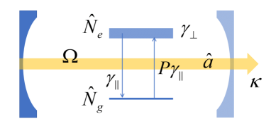
Figure 1: Scheme of the two-level laser. Upper levels of emitters with the population operator $\hat{N}_{e}$, decay to the low levels with the rate $\gamma_{\parallel}$ and pumped with the rate $\gamma_{\parallel}P$ from the low levels with the population $\hat{N}_{g}$. The width of the lasing transition is $\gamma_{\perp}$. Lasing mode described by Bose-operator $\hat{a}$ decays through the semitransparent mirror with the rate $\kappa$ and resonantly interacts with lasing transitions of two-level emitters with the vacuum Rabi frequency $\Omega$.

Lasing transitions are in resonance with the cavity mode of the optical carrier frequency $\omega_{0}$. $\hat{a}(t){{e}^{-i{{\omega}_{0}}t}}$ is the cavity mode Bose-operator with the complex amplitude $\hat{a}(t)$ changed much more slowly than ${{e}^{-i{{\omega}_{0}}t}}$.

Hamiltonian of the laser, written in the interaction picture and in the RWA approximation with the carrier frequency $\omega_{0}$, is

$$H=i\hbar\Omega\sum\limits_{i=1}^{{{N}_{0}}}{{{f}_{i}}\left({{{\hat{a}}}^{+}}{{{\hat{\sigma}}}_{i}}-\hat{\sigma}_{i}^{+}\hat{a}\right)}+\hat{\Gamma}.$$ (1)

Here $\Omega$ is the vacuum Rabi frequency, $\Omega f_{i}$ with the dimensionless factor $f_{i}$ describes the coupling of i-th emitter with the cavity mode; $\hat{\sigma}_{i}$ is a lowing operator of i-th emitter, $\hat{\Gamma}$ describes the dissipation due to the interaction of the mode and emitters with the environment.

Commutation relations for operators in the Hamiltonian (1) are

$$\left[\hat{a},{{{\hat{a}}}^{+}}\right]=1,\hskip 7.11317pt\left[{{{\hat{\sigma}}}_{i}},\hat{\sigma}_{j}^{+}\right]=\left(\hat{n}_{i}^{g}-\hat{n}_{i}^{e}\right){{\delta}_{ij}},\hskip 7.11317pt\left[{{{\hat{\sigma}}}_{i}},\hat{n}_{j}^{e}\right]=\left[\hat{n}_{j}^{g},{{{\hat{\sigma}}}_{i}}\right]={{\delta}_{ij}}{{\hat{\sigma}}_{i}},$$ (2)

where $\hat{n}_{j}^{e}$ and $\hat{n}_{j}^{g}$ are operators of populations of the upper and the low states of i-th emitter, $\delta_{ij}$ is Kronecker symbol.

We introduce operators $\hat{v}$ and $\hat{N}_{e,g}$ of the polarization and populations of all emitters

$$\hat{v}=\sum\limits_{i=1}^{{{N}_{0}}}{{{f}_{i}}{{{\hat{\sigma}}}_{i}}}\hskip 28.45274pt{{\hat{N}}_{e,g}}=\sum\limits_{i=1}^{{{N}_{0}}}{\hat{n}_{i}^{e,g}}.$$ (3)

Using commutation relations (2) and Hamiltonian (1) we write Maxwell-Bloch equations (MBE) for $\hat{a}$, $\hat{v}$ and ${\hat{N}}_{e}$. It is convenient to express MBE with the population fluctuations. We take $\hat{N}_{e}=N_{e}+\delta\hat{N}_{e}$, where $N_{e}$ is the mean value of $\hat{N}_{e}$ and $\delta\hat{N}_{e}$ describes fluctuations. We use letters with ”hats” for operators and letters without ”hats” for the mean values, for example, the mean value $\left<\hat{N}_{e}\right>\equiv N_{e}$.

MBE with the population fluctuations are

$$\dot{\hat{a}} = -\kappa\hat{a}+\Omega\hat{v}+{{{\hat{F}}}_{a}}$$ (4a)

$$\dot{\hat{v}} = -\left({{\gamma}_{\bot}}/2\right)\hat{v}+\Omega f\hat{a}\left(N+2{{\delta{\hat{N}}}_{e}}\right)+{{{\hat{F}}}_{v}}$$ (4b)

$$\delta{{{\dot{\hat{N}}}}_{e}} = -\Omega\delta\hat{\Sigma}-{{\gamma}_{P}{{\delta{\hat{N}}}_{e}}}+{{{\hat{F}}}_{N_{e}}}.$$ (4c)

Here

$${\gamma}_{P}={\gamma}_{\parallel}(P+1),$$ (5)

$\kappa$, ${\gamma}_{\bot}$ and ${\gamma}_{\parallel}$ are the cavity mode, the polarization and the population decay rates, correspondingly; $P$ is the dimensionless pump rate, $N=N_{e}-N_{g}$ is the mean population inversion, ${{\hat{F}}_{\alpha}}$ with the index $\alpha=\left\{a,v,{{N}_{e}}\right\}$ are the Langevin force operators. The total number of emitters is preserved, so ${\hat{N}}_{e}+{\hat{N}}_{g}={N}_{0}$. In Eqs. (4) $\delta\hat{\Sigma}$ means fluctuations of the operator $\hat{\Sigma}\equiv{{\hat{a}}^{+}}\hat{v}+{{\hat{v}}^{+}}\hat{a}$ and we approximate $f_{i}^{2}\approx f=N_{0}^{-1}\sum\limits_{i=1}^{{{N}_{0}}}{f_{i}^{2}}$.

Eqs. (4) are consistent and must be solved together with the energy conservation law

$$2\kappa n=\gamma_{\parallel}[P(N_{0}-N_{e})-N_{e}],$$ (6)

where the mean photon number $n=\left<\hat{a}^{+}\hat{a}\right>$. The operator $\hat{a}$ is found from Eqs. (4) as a function of the unknown $N_{e}$, then $n$ is calculated using $\hat{a}$ and then $N_{e}$ is found from the energy conservation law (6). Population fluctuations $\delta\hat{N}_{e}$ can be found, for example, by the perturbation procedure [17].

Some approximations help to solve Eqs. (4). In a ”zero-order” approximation, denoted below by the index ”0”, we neglect population fluctuations, drop $\delta\hat{N}_{e}$ in Eq. (4b) and write

$$\dot{\hat{a}}_{0} = -\kappa\hat{a}_{0}+\Omega\hat{v}_{0}+{{{\hat{F}}}_{a}}$$ (7a)

$$\dot{\hat{v}}_{0} = -\left({{\gamma}_{\bot}}/2\right)\hat{v}_{0}+\Omega f\hat{a}_{0}N+{{{\hat{F}}}_{v}^{(0)}},$$ (7b)

We replace the Langevin force $\hat{F}_{v}$ by $\hat{F}_{v}^{(0)}$ in Eq. (4b); such a replacement is necessary for preserving Bose commutation relations for $\hat{a}_{0}$ and commutation relations

$$\left<[\hat{v}_{0},\hat{v}_{0}^{+}]\right>=f(N_{g}-N_{e})$$ (8)

at zero-order approximation. Commutation relations (8) follow from Eqs. (2). The Langevin force $\hat{F}_{a}$ remains the same in the exact Eqs. (4) and in the zero-order approximation Eqs. (7), $\hat{F}_{a}$ corresponds to the field decay through the Fabry-Perot cavity semi-transparent mirror [24, 25]. Eqs. (7) can be derived from the ”oscillator laser model” [26].

Eqs. (7) are linear in $\hat{a}_{0}$ and $\hat{v}_{0}$ and can be solved by the Fourier-transform $\hat{\alpha}(t)=(2\pi)^{-1/2}\int_{-\infty}^{\infty}{\hat{\alpha}(\omega)}e^{-i\omega t}d\omega$, where $\hat{\alpha}$ means $\hat{a}_{0},\hat{v}_{0},\hat{F}_{a}...$, $\hat{\alpha}(\omega)$ is the Fourier-component operator. Fourier-component operators obtained from Eqs. (7) are

$$\hat{a}_{0}(\omega) = [\left({{\gamma}_{\bot}}/2-i\omega\right){{{\hat{F}}}_{a}}(\omega)+\Omega{{{\hat{F}}}_{v}}^{(0)}(\omega)]/s(\omega)$$ (9a)

$$\hat{v}_{0}(\omega) = [\left(\kappa-i\omega\right){{{\hat{F}}}_{v}^{(0)}}(\omega)+\Omega fN\hat{F}_{a}(\omega)]/s(\omega)$$ (9b)

where

$$s(\omega)=\left(i\omega-\kappa\right)\left(i\omega-{{\gamma}_{\bot}}/2\right)-(\kappa\gamma_{\perp}/2)N/N_{th}.$$ (10)

In Eq. (10) $N_{th}=\kappa\gamma_{\perp}/2f\Omega^{2}$ is the lasing threshold population inversion found in the semi-classical laser theory [23]. $N_{th}^{-1}\geq 1$ means a strong emitter-field coupling, when the emitter-field interaction became reversible, leading to the change in the emitted field spectrum structure, in particular, to Rabi splitting [27].

An important factor in the laser MBE is the non-adiabatic parameter $2\kappa/\gamma_{\perp}$. In the limit $2\kappa/\gamma_{\perp}\rightarrow 0$ one can eliminate the polarization $\hat{v}$ from Eqs. (4) adiabatically and reduce Eqs. (4) to the laser rate equations. When $2\kappa/\gamma_{\perp}\geq 1$ the non-adiabatic polarization dynamics is important and leads, in particular, to collective effects.

The relation $\left<\hat{F}_{\alpha}(\omega)\hat{F}_{\beta}(\omega^{\prime})\right>=2D_{\alpha\beta}\delta(\omega+\omega^{\prime})$ determines the power spectrum (or the diffusion coefficient) $2D_{\alpha\beta}$ for the Langevin forces $\hat{F}_{\alpha}(\omega)$, $\hat{F}_{\beta}(\omega^{\prime})$. The power spectra for the Langevin forces in the zero-order approximation Eqs. (7) are

$$2D_{v^{+}v}^{(0)}=f{{\gamma}_{\bot}}{N}_{e},\hskip 14.22636pt2D_{vv^{+}}^{(0)}=f{{\gamma}_{\bot}}{N}_{g},\hskip 14.22636pt2D_{a^{+}a}=0,\hskip 14.22636pt2D_{aa^{+}}=2\kappa,$$ (11)

It is convenient to represent the Langevin force $\hat{F}_{v}$ in Eq. (4b) as a sum

$$\hat{F}_{v}=\hat{F}_{v}^{(0)}+\hat{F}_{v}^{(N)},$$ (12)

where $\hat{F}_{v}^{(N)}$ describes the polarization noise due to population fluctuations. We suppose a large number of emitters $N_{0}\gg 1$, each emitter interacts with its own bath uncorrelated with the baths of other emitters. In this case, we neglect the correlations between $\hat{F}_{v}^{(0)}$ and $\hat{F}_{v}^{(N)}$ in a good approximation with a precision $\sim N_{0}^{-1}$.

It is shown in Appendix A that the Langevin force

$$\hat{F}_{v}^{(N)}=2\Omega f\hat{b}_{in}^{+}\delta\hat{N}_{e}$$ (13)

where $\hat{b}_{in}$ is an amplitude Bose-operator of the vacuum field bath of ”inverted” oscillators responsible for the spontaneous emission to the cavity mode. The Bose-operator of the inverted oscillator mode is $\hat{b}_{in}(\omega)e^{i\omega_{0}t}$. Note the sign $"+"$ is in $e^{i\omega_{0}t}$ for the inverted oscillator, while it is $e^{-i\omega_{0}t}$ for the usual oscillator. Inverted oscillator bath has been introduced in [28] and used for the theoretical description of quantum amplifiers [29] and lasers [26].

The power spectra of $\hat{b}_{in}$ are found in Appendix A, they are

$$\left<\hat{b}_{in}^{+}(\omega)\hat{b}_{in}(\omega^{\prime})\right>=0,\hskip 14.22636pt\left<\hat{b}_{in}(\omega)\hat{b}_{in}^{+}(\omega^{\prime})\right>=c(\omega)\delta(\omega+\omega^{\prime}),$$ (14)

where

$$c(\omega)=\frac{2\kappa{{\omega}^{2}}+(\kappa\gamma_{\bot}^{2}/2)(1-N/N_{th})}{{{\left|s(\omega)\right|}^{2}}},$$ (15)

We see that $(2\pi)^{-1}\int_{-\infty}^{\infty}c(\omega)d\omega=1$, so Bose commutation relations $\left<[\hat{b}_{in}(t),\hat{b}^{+}_{in}(t)]\right>=1$ are satisfied. In a difference with the well-known pump bath of inverted oscillators with a ”white” (i.e. with a frequency independent power density) spectrum [28, 29], we use a ”colored” bath with $c(\omega)$ power density. Such a ”colored” bath is formally necessary for providing Bose-commutation relations for $\hat{a}$ with the population fluctuations taken into account, as shown in Appendix A. Physically the colored bath is related with the spontaneous emission to the cavity mode.

The power spectrum of the operator product $\hat{b}_{in}^{+}\delta N_{e}$ is a convolution of the power spectra of the multipliers in the product [17]. So the power spectrum of $\hat{F}_{v}^{(N)}(\omega)$, given by Eq. (13), is

$$2D_{{{v}^{+}}v}^{(N)}(\omega)=f{{\gamma}_{\bot}}(\kappa/{{N}_{th}}){{\left(c*{{\delta}^{2}}{{N}_{e}}\right)}_{\omega}},\hskip 28.45274pt2D_{v{{v}^{+}}}^{(N)}(\omega)=0$$ (16)

where $\left(c*\delta^{2}N_{e}\right)_{\omega}$ is a convolution of $c(\omega)$ and the population fluctuation spectrum ${{\delta}^{2}}{{N}_{e}}(\omega)$. It is shown in Appendix that the Langevin force $\hat{F}_{v}^{(N)}(\omega)$ determined by relations (13) – (15) preserves Bose commutation relations for $\hat{a}$ and commutation relations $\left<[\hat{v},\hat{v}^{+}]\right>=f(N_{g}-N_{e})$ for $\hat{v}$.

The power spectrum for the population fluctuation Langevin force $\hat{F}_{N_{e}}$ is

$$2D_{N_{e}N_{e}}=\gamma_{\parallel}(PN_{g}+N_{e}),$$ (17)

it is the same as in the rate equation laser theory [30], which is a good approximation for a large number of emitters.

III the cavity field spectrum and the mean photon number

It was found in [17] that the population fluctuations increase the cavity mode spontaneous emission and the mean photon number $n$. Here we represent the results of [17] in the form convenient for calculations of $g_{2}$, derive analytical expression for $n$ and show conditions, when the population fluctuations noticeable increase $n$. We use results of this section for calculations of $g_{2}$.

An expression (36) for $\hat{a}(\omega)$ is given in Appendix A. Substituting $\hat{a}(\omega)$ from Eq. (36) to

$$\left<(\hat{a}^{+})_{\omega}\hat{a}(\omega^{\prime})\right>=n(\omega)\delta(\omega+\omega^{\prime})$$ (18)

we obtain the integral equation for $n(\omega)$ with unknown population fluctuation spectrum $\delta^{2}N_{e}(\omega)$ and $N_{e}$. $\delta^{2}N_{e}(\omega)$ can be found, for example, by a perturbation procedure described in [17]. Then we calculate $n(\omega)$, $n=(2\pi)^{-1}\int_{-\infty}^{\infty}n(\omega)d\omega$ and determine $N_{e}$ from the energy conservation law (6).

In this paper we restrict ourselves by a weak pump and a linear radiation regime, when the change of the population due to the cavity field is negligibly small. In the linear regime we drop the term with $\hat{a}$ in Eq. (36). We removed from Eq. (36) the term with $\hat{F}_{a}$, because of it does not contribute to the final results. So we use

$$\hat{a}(\omega)=\frac{\Omega\hat{F}_{v}^{(0)}(\omega)+(\kappa\gamma_{\bot}/N_{th})\left(\hat{b}_{in}^{+}\delta\hat{N}_{e}\right)_{\omega}}{s(\omega)}$$ (19)

in the calculations below. In the linear regime we drop $\Omega\delta\hat{\Sigma}(\omega)$ in Eq. (35c), find $\delta\hat{N}_{e}(\omega)=\hat{F}_{N_{e}}(\omega)/(i\omega-\gamma_{P})$ and the population fluctuation power spectrum

$$\delta^{2}{N}_{e}(\omega)=\delta^{2}{N}_{e}L(\omega,\gamma_{P}),$$ (20)

where $\gamma_{P}$ is given by Eq. (5),

$$L(\omega,\gamma)=2\gamma/(\omega^{2}+\gamma^{2})$$ (21)

is a Lorenz spectrum with the half-width $\gamma$; $(2\pi)^{-1}\int_{-\infty}^{\infty}L(\omega,\gamma)d\omega=1$. The upper state population fluctuation dispersion and the mean population of the upper emitter states are

$$\delta^{2}{N}_{e}=N_{e}/(P+1),\hskip 14.22636ptN_{e}=PN_{0}/(P+1).$$ (22)

In calculations of $\delta^{2}{N}_{e}$ we use the population fluctuation power spectrum (17).

We substitute $\hat{a}(\omega)$ from Eq. (19) and the Fourier-component $(\hat{a}^{+})_{\omega}\equiv\hat{a}^{+}(-\omega)$ to Eq. (18) for $n(\omega)$, neglect by correlations between $\hat{F}_{v}^{(0)}(\omega)$ and $\left(\hat{b}_{in}^{+}\delta\hat{N}_{e}\right)_{\omega}$ and find $n(\omega)$ in the weak pump limit. The power spectrum $S_{bN_{e}}(\omega)$ of the operator product $\hat{b}_{v}\delta\hat{N}_{e}$ is

$$S_{bN_{e}}(\omega)\equiv(c*\delta^{2}N_{e})_{\omega}=\frac{1}{2\pi}\int_{-\infty}^{\infty}c(\omega-\omega^{\prime})\delta^{2}N_{e}(\omega^{\prime})d\omega^{\prime}.$$ (23)

The spectra $c(\omega)$ and $\delta^{2}{N}_{e}(\omega)$ are given by Eq. (15) and Eq. (20), correspondingly.

We simplify the integral (23) by noting that the width of $c(\omega)$ spectrum is $\sim\sqrt{\kappa\gamma_{\perp}}\gg\gamma_{P}\approx\gamma_{\parallel}$, which is the width of the population fluctuation spectrum $\delta^{2}N_{e}(\omega)$. So we approximate

$$(c*\delta^{2}N_{e})_{\omega}\approx c(\omega)\delta^{2}N_{e}$$ (24)

at the condition

$$\gamma_{\parallel}/\sqrt{\kappa\gamma_{\perp}}\ll 1.$$ (25)

Inserting $\hat{a}(\omega)$ from Eq. (19) to $\left<(\hat{a}^{+})_{\omega}\hat{a}(\omega^{\prime})\right>=n(\omega)\delta{(\omega+\omega^{\prime})}$ we find the photon number spectrum

$$n(\omega)=\frac{\left(\kappa\gamma_{\bot}^{2}/2{{N}_{th}}\right){{N}_{e}}+\delta^{2}N_{e}{{(\kappa{{\gamma}_{\bot}}/{{N}_{th}})}^{2}}c(\omega)}{{{\left|s(\omega)\right|}^{2}}}.$$ (26)

Fig. 2 shows examples of $n(\omega)$. The double-peak structure of $n(\omega)$ is due to the collective Rabi splitting [22]. The solid curves are with and the dashed curves are without population fluctuations.

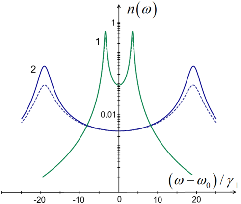
Figure 2: Photon number spectrum in a weak pump regime with $P=0.1$, strong field-emitter coupling $N_{th}=1$ and good $2\kappa/\gamma_{\perp}=0.2$ (curves 1) or bad $2\kappa/\gamma_{\perp}=6$ (curves 2) cavities; here and below $\gamma_{\parallel}/\gamma_{\perp}=0.1$. Solid (dashed) curves are with (without) population fluctuations. Population fluctuations noticeable increase the spectrum maxima for the bad cavity and practically have no effect on the good cavity spectrum. The two maxima are due to the collective Rabi splitting [22]. Population fluctuations do not change a position of the maxima.

Population fluctuations do not change the positions of the spectrum maxima and increase the height of maxima for the bad cavity (curves 2). Population fluctuations practically have no effect on the good cavity photon spectra (curves 1).

We take Eq. (26) and calculate the mean photon number

$$n=\frac{1}{2\pi}\int_{-\infty}^{\infty}n(\omega)d\omega=n_{0}+\delta^{2}N_{e}\left(\frac{\kappa\gamma_{\perp}}{N_{th}}\right)^{2}\frac{1}{2\pi}\int_{-\infty}^{\infty}\frac{c(\omega)}{{{\left|s(\omega)\right|}^{2}}}d\omega.$$ (27)

We calculate the integral in Eq. (27), make some algebraic transformations and find

$$n=n_{0}\left(1+\Delta_{n}\right),\hskip 14.22636pt\Delta_{n}=\frac{\delta^{2}N_{e}}{N_{e}}\frac{1}{N_{th}}\left[3\left(\frac{2\kappa/\gamma_{\perp}}{1+2\kappa/\gamma_{\perp}}\right)^{2}+\frac{2\kappa/\gamma_{\perp}}{1-N/N_{th}}\right]$$ (28)

where $\Delta_{n}$ is a relative increase of $n$ caused by population fluctuations and

$$n_{0}=\frac{{{N}_{e}}}{\left(1+2\kappa/{{\gamma}_{\bot}}\right)\left({{N}_{th}}-N\right)}$$ (29)

is a part of the mean photon number found without population fluctuations from the zero-order approximation equations (7); $n_{0}$ is the same as in [22, 17, 23]. According with Eqs. (22) ${\delta^{2}N_{e}}/{N_{e}}=1/(P+1)\approx 1$ for a weak pump $P\ll 1$.

The expression (28) shows that the population fluctuations noticeably increase $n$ at small $N_{th}$, which means a strong field-emitter coupling; and for a bad cavity, when the non-adiabatic parameter is large, $2\kappa/\gamma_{\perp}>1$, which is typical for the super-radiant LEDs and lasers. The result of $\Delta_{n}$ will be used in the calculations of $g_{2}$ in the next section.

Fig. 3 shows $\Delta_{n}$ as a function of $2\kappa/\gamma_{\perp}$ at various $N_{th}$.

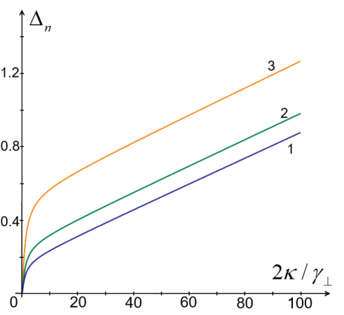
Figure 3: The relative increase $\Delta_{n}$ of the cavity photon number is due to the population fluctuations at a weak pump regime at $P=0.1$ and $\gamma_{\parallel}/\gamma_{\perp}=0.1$ as a function of the non-adiabatic parameter $2\kappa/\gamma_{\perp}$ at $N_{th}=15$ (curve 1), $10$ (2) and $5$ (3).

IV the super-thermal photon statistics

We use the expression (19) for calculations of the second-order auto-correlation function $g_{2}=\left<\hat{a}^{+}(t)\hat{a}^{+}(t)\hat{a}(t)\hat{a}(t)\right>/n^{2}$. Making the Fourier-expansion we write

$$g_{2}=\frac{1}{n^{2}}\frac{1}{(2\pi)^{2}}\int_{-\infty}^{\infty}\left<(\hat{a}^{+})_{\omega_{1}}(\hat{a}^{+})_{\omega_{2}}\hat{a}(\omega_{3})\hat{a}(\omega_{4})\right>e^{-i(\omega_{1}+\omega_{2}+\omega_{3}+\omega_{4})t}d\omega_{1}d\omega_{2}d\omega_{3}d\omega_{4}.$$ (30)

We will see that $\left<(\hat{a}^{+})_{\omega_{1}}(\hat{a}^{+})_{\omega_{2}}\hat{a}(\omega_{3})\hat{a}(\omega_{4})\right>\neq 0$ at $\omega_{1}+\omega_{2}+\omega_{3}+\omega_{4}=0$, as it must be in the stationary regime, so we drop the exponent multiplier in (30) and write

$$g_{2}=\frac{1}{n^{2}}\frac{1}{(2\pi)^{2}}\int_{-\infty}^{\infty}\left<(\hat{a}^{+})_{\omega_{1}}(\hat{a}^{+})_{\omega_{2}}\hat{a}(\omega_{3})\hat{a}(\omega_{4})\right>d\omega_{1}d\omega_{2}d\omega_{3}d\omega_{4}.$$ (31)

We calculate $\left<(\hat{a}^{+})_{\omega_{1}}(\hat{a}^{+})_{\omega_{2}}\hat{a}(\omega_{3})\hat{a}(\omega_{4})\right>$, take the integral in Eq. (31) and obtain $g_{2}$.

Substituting the expression (19) for $\hat{a}(\omega)$ to Eq. (31) and neglecting by correlations between $\hat{F}_{v}^{(0)}(\omega)$ and $\left(\hat{b}_{in}^{+}\delta\hat{N}_{e}\right)_{\omega}$ we find

$$g_{2}=2+\left(\frac{\kappa\gamma_{\perp}}{N_{th}}\right)^{4}\frac{C_{g}}{n^{2}}$$ (32)

where $C_{g}$ is a cumulant for the operator $\hat{B}(\omega)=\left(\hat{b}_{in}^{+}\delta\hat{N}_{e}\right)_{\omega}/s(\omega)$:

$$C_{g}=\frac{1}{(2\pi)^{2}}\int_{-\infty}^{\infty}\left<(\hat{B}^{+})_{\omega_{1}}(\hat{B}^{+})_{\omega_{2}}\hat{B}(\omega_{3})\hat{B}(\omega_{4})\right>d\omega_{1}...d\omega_{4}$$

$$-2\left[\frac{1}{2\pi}\int_{-\infty}^{\infty}\left<(\hat{B}^{+})_{\omega_{1}}\hat{B}(\omega_{2})\right>d\omega_{1}d\omega_{2}\right]^{2}.$$ (33)

Here

$$\left<(\hat{B}^{+})_{\omega_{1}}\hat{B}(\omega_{2})\right>=\frac{S_{bN_{e}}(\omega)}{|s(\omega)|^{2}}\delta(\omega_{1}+\omega_{2})$$

and the spectrum $S_{bN_{e}}(\omega)$ of the operator product $\hat{b}_{in}^{+}\delta\hat{N}_{e}$ is determined by Eq. (23). Calculations of $C_{g}$ and some algebraic transformations shown in Appendix B lead to the result

$$g_{2}=2\left[1+2\left(\frac{\Delta_{n}}{1+\Delta_{n}}\right)^{2}\right],$$ (34)

where the relative change in the cavity photon number due to population fluctuations $\Delta_{n}$ is given by Eq. (28). The result (34) is found in the approximation (24) at the condition (25).

Fig. 4 shows

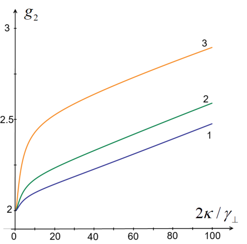
Figure 4: $g_{2}$ at a weak pump $P=0.1$ as a function of the non-adiabatic parameter $2\kappa/\gamma_{\perp}$ for $N_{th}=15$ (curve 1), $10$ (curve 2) and $5$ (curve 3).

$g_{2}$ as a function of the non-adiabatic parameter $2\kappa/\gamma_{\perp}$ at various $N_{th}$.

Fig. 5 shows $g_{2}$ as a function of the dimensionless pump $P$ for various $2\kappa/\gamma_{\perp}$ and $N_{th}$.

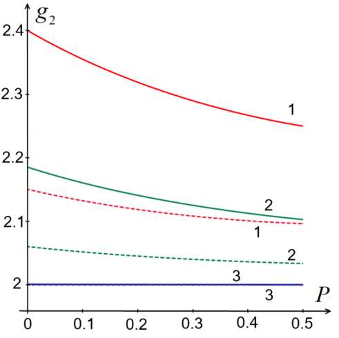
Figure 5: $g_{2}$ as a function of the dimensionless pump $P$ for the non-adiabatic parameter $2\kappa/\gamma_{\perp}=6$ (curves 1), $2$ (curves 2) and $0.2$ (curves 3). $N_{th}=5$ for the solid curves and $10$ for dashed curves.

We see that the maximum $g_{2}$ at $P\rightarrow 0$ is increased with $2\kappa/\gamma_{\perp}$, decreased with $N_{th}$ and $g_{2}(P)$ is reduced with $P$. Such a reduction is because of the relative population fluctuation dispersion is decreased with $P$: $\delta^{2}N_{e}/N_{e}=1/(P+1)$. The $g_{2}(P)$ dependence at large $P\geq 1$ must be studied using the nonlinear equations (4) taking into account the population fluctuations and the stimulated emission to the lasing mode.

V Discussion of results

We use the result of [17] that population fluctuations increase the mean photon number at conditions seen in Eq. (28) for $\Delta_{n}$. The relative mean photon number increase $\Delta_{n}$ is large, when $N_{th}$ is small, which means a strong emitter-field coupling. In our examples we take $N_{th}\geq 1$ as $N_{th}=5$, $10$ and $15$ in Figs. 3 and 4. Formula (28) tells, that $\Delta_{n}$ can be even larger than on Figs. 3 and 4, if we take $N_{th}<1$. A value $N_{th}<1$ can be achieved, for example in the photonic crystal laser with the quantum dot active medium and a small cavity mode volume $V\sim(\lambda/2)^{3}$, where $\lambda$ is the optical or near-IR wavelength of the cavity mode field. However, we must be careful with the use of the formula (28) at $N_{th}<1$. For $N_{th}<1$ the spontaneous emission rate $\gamma_{sp}$ to the cavity mode is so large, that it gives a noticeable contribution to the emitter transition width $\gamma_{\perp}$. Our analysis is done on the assumption $\gamma_{sp}\ll\gamma_{\perp}$, which is true for $N_{th}>1$. The analysis for $\gamma_{\perp}\sim\gamma_{sp}$ will be carried out in the future.

The second condition necessary for the increase of $\Delta_{n}$ is a large non-adiabatic parameter $2\kappa/\gamma_{\perp}>1$, when the collective effects, as a sub- or super-radiance to the cavity mode, are significant [19, 20, 21]. There is a physical explanation of why collective effects lead to the increase of $n$ due to population fluctuations. Suppose, we have $N_{0}$ independent emitters (dipoles) and no collective effects in the radiation. The mean radiation power from an independent emitters is proportional to the number $N_{e}$ of the emitters in the upper states, fluctuations $\delta N_{e}$ do not contribute to the mean number $n$ of emitted photons $n\sim\left<N_{e}+\delta N_{e}\right>=N_{e}$. This is not the case for the collective emission, when at least a part of $n$ is proportional to $\left<(N_{e}+\delta N_{e})^{2}\right>=N_{e}^{2}+\left<(\delta N_{e})^{2}\right>$, so the population fluctuations contribute to the mean photon number.

By noting the term $\sim\hat{a}\delta\hat{N}_{e}$ in Eq. (4b) we see, that the population fluctuations increase the stimulated emission. In this paper we consider the population fluctuations increase of the spontaneous emission to the cavity mode. The population fluctuation contribution to the spontaneous emission is described by the Langevin force (13) with the power spectrum (16). The Langevin force (13) has been found from the requirement of Bose commutation relations for $\hat{a}$ at the population fluctuations. Now we give an explanation of the physics described by the Langevin force (13). The emitters in the upper states can be represented as inverted harmonic oscillators [26]. We assume, that the inverted oscillators interact with the bath of the inverted vacuum field modes $\hat{b}_{in}(\omega)e^{+i\omega_{0}t}$, $\left<\hat{b}_{in}^{+}(\omega)\hat{b}_{in}(\omega^{\prime})\right>=0$, by analogy as ”normal” oscillators interact with the usual vacuum field modes. The field operators $\hat{b}_{in}(\omega)$ are Bose-operators, so the commutation relations $[\hat{b}_{in}(\omega),\hat{b}_{in}(\omega^{\prime})]=c(\omega)\delta(\omega+\omega^{\prime})$ with $(2\pi)^{-1}\int_{-\infty}^{\infty}c(\omega)d\omega=1$. $\hat{b}_{in}(\omega)e^{+i\omega_{0}t}$ are the cavity modes, this is why their commutator power spectrum is not a unity, as in the free space, but $c(\omega)$ given by Eq. (15). We present the oscillator laser model with the inverted oscillator vacuum field bath $\hat{b}_{in}$ and the population fluctuations in the forthcoming paper.

In our model, the super-thermal photon statistics with $g_{2}>2$ is caused by the population fluctuation effect on the radiation. If we neglect the population fluctuations we obtain $g_{2}=2$ [22, 23]. $g_{2}$ grows with the adiabatic parameter $2\kappa/\gamma_{\perp}$, see Fig. 4 and noticeably increases above 2, when $2\kappa/\gamma_{\perp}$ is large and collective effects are significant, which is in accordance with several results [12, 31, 18]. Proceeding calculations we see that $g_{2}>2$ it is because of $\hat{a}\sim\delta\hat{N}_{e}$. The population fluctuations $\delta\hat{N}_{e}$ do not have a phase, therefore $\left<(\delta\hat{N}_{e})^{4}\right>\sim 3\left<\delta\hat{N}_{e}^{2}\right>^{2}$. Otherwise, if we neglect the population fluctuations, then $\left<\hat{a}^{+}\hat{a}^{+}\hat{a}\hat{a}\right>\sim 2n^{2}$ leads to $g_{2}=2$. This is a rough explanation of why we have $g_{2}>2$ due to the population fluctuations. Quantitative consideration of $g_{2}$ and the calculations of the cumulant (33) with the population fluctuations is shown in Appendix B.

We derived a simple analytical formula (34) for $g_{2}$. Eq. (34) predicts $g_{2}\rightarrow 6$ at $\Delta_{n}\gg 1$. However, the broadening of the emitter transition by the cavity mode spontaneous emission makes it difficult to achieve $\Delta_{n}\gg 1$. The estimation of the maximum value of $g_{2}$ in our model requires more studies, taking into account the broadening of the emitter transition by the cavity mode spontaneous emission. The maximum $g_{2}$ in our model is, anyway, no more than $g_{2}=6$. Some graphs with $g_{2}>2$ at various parameters are shown in Fig. 4.

Using our results, one can suggest that a large $g_{2}$ means a large population fluctuations and an increase in the radiation due to the population fluctuations.

Population fluctuations considered here come from a fast and random transition of the emitters from the low to the upper states due to the pump process, for example, the pump by the external current. Another population fluctuation mechanism is the fluctuations in the field-emitter interaction from one emitter to another described by the factor $f_{i}$ in the Hamiltonian (1). We do not consider such fluctuations here, replacing $f_{i}^{2}$ with its mean value $f=1/2$. It is possible, that the contribution of such fluctuations increases $g_{2}$. Another physical mechanisms, but the population fluctuations, may cause the super-thermal photon statistics and $g_{2}>2$.

VI Conclusion

We show that the population fluctuations in the two-level LED model increase the mean photon number and lead to the super-thermal photon statistics for a strong field-emitter coupling and a bad LED cavity, favorable for collective effects in the LED. Analytical formulas for the mean photon number and the second-order auto-correlation function $g_{2}$, depending on the population fluctuations, are found. The results can be used for understanding of the physics of work of a small LED and lasers with only a few photons in the cavity and for the increase of the LED radiation efficiency by population fluctuations.

Appendix A Correlation properties of the Langevin force $\hat{F}^{(N)}_{v}$

Here we prove that the power spectra of $\hat{b}_{in}$ is given by Eq. (14) and find the power spectrum Eq. (16) for $\hat{F}^{(N)}_{v}$.

Making the Fourier-expansion of operators in Eqs. (4) we come to algebraic equations for Fourier-component operators

$$0 = \left(i\omega-\kappa\right)\hat{a}(\omega)+\Omega\hat{v}(\omega)+{{{\hat{F}}}_{a}}(\omega)$$ (35a)

$$0 = \left(i\omega-{{\gamma}_{\bot}}/2\right)\hat{v}(\omega)+\Omega f\left[\hat{a}(\omega)N+2{{\left(\hat{a}\delta{{{\hat{N}}}_{e}}\right)}_{\omega}}\right]+{{{\hat{F}}}_{v}^{(0)}}(\omega)+{{{\hat{F}}}_{v}^{(N)}}(\omega).$$ (35b)

$$0 = (i\omega-\gamma_{P})\delta\hat{N}_{e}(\omega)-\Omega\delta\hat{\Sigma}(\omega)+\hat{F}_{N_{e}}(\omega),$$ (35c)

We find from Eqs. (35a), (35b) taking into account the expression (13) for $\hat{F}_{v}^{(N)}$

$$\hat{a}(\omega)=\hat{a}_{0}(\omega)+\frac{\kappa{{\gamma}_{\bot}}}{{N}_{th}s(\omega)}\hat{d}(\omega),\hskip 14.22636pt\hat{v}(\omega)=\hat{v}_{0}(\omega)+\frac{2f\Omega\left(\kappa-i\omega\right)}{s(\omega)}\hat{d}(\omega)$$ (36)

where the Fourier-component $\hat{d}(\omega)=\left[\left(\hat{a}+\hat{b}_{in}^{+}\right)\delta{\hat{N}_{e}}\right]_{\omega}$ and $\hat{a}_{0}(\omega)$, $\hat{v}_{0}(\omega)$ are solutions (9) of the zero-order approximation equations (7). Using Eqs. (9) and the zero-order diffusion coefficients (11) we see that

$$\left<[\hat{a}_{0}(\omega),\hat{a}_{0}^{+}(\omega^{\prime})]\right>=c(\omega)\delta(\omega+\omega^{\prime})$$ (37)

where $c(\omega)$ is a commutator spectrum given by Eq. (15). The integral $(2\pi)^{-1}\int_{-\infty}^{\infty}c(\omega)d\omega=1$ provides Bose commutation relations $[\hat{a}_{0}(t),\hat{a}_{0}^{+}(t)]=1$ for $\hat{a}_{0}(t)$. The same Bose commutation relations must be hold for $\hat{a}(t)$

$$[\hat{a}(t),\hat{a}^{+}(t)]=1.$$ (38)

We use the condition Eq. (38) for finding $\hat{b}_{in}$. Taking $\hat{a}(\omega)$ given by Eq. (36) we write the Fourier-component commutator

$$\left<[\hat{a}(\omega),(\hat{a}^{+})_{\omega^{\prime}}]\right>=c(\omega)\delta(\omega+\omega^{\prime})+\theta(\omega,\omega^{\prime})$$ (39)

where

$$\theta(\omega,\omega^{\prime})=\frac{\kappa\gamma_{\perp}}{N_{th}}\left\{\frac{\left<[\hat{d}(\omega),(\hat{a}_{0}^{+})_{\omega^{\prime}}]\right>}{s(\omega)}+\frac{\left<[\hat{a}_{0}(\omega),(\hat{d}^{+})_{\omega^{\prime}}]\right>}{s^{*}(-\omega^{\prime})}\right\}+\left(\frac{\kappa\gamma_{\perp}}{N_{th}}\right)^{2}\frac{\left<[\hat{d}(\omega),(\hat{d}^{+})_{\omega^{\prime}}]\right>}{s(\omega)s^{*}(-\omega^{\prime})}$$ (40)

We integrate Eq. (39) over $d\omega$ and $d\omega^{\prime}$, taking into accoint $(2\pi)^{-1}\int_{-\infty}^{\infty}c(\omega)d\omega=1$, and see, that Bose commutation relations (38) are satisfied, if we find $\hat{b}_{in}$ such that $\theta(\omega,\omega^{\prime})=0$. Suppose, we have found such $\hat{b}_{in}$. Then

$$\left<[\hat{a}_{0}(\omega),(\hat{a}_{0}^{+})_{\omega^{\prime}}]\right>=\left<[\hat{a}(\omega),(\hat{a}^{+})_{\omega^{\prime}}]\right>=c(\omega)\delta(\omega+\omega^{\prime})$$ (41)

which means that Bose commutation relations for the cavity mode operator do not depend on the population fluctuations in our model.

Let us find $\hat{b}_{in}$ such that $\theta(\omega,\omega^{\prime})=0$. The first term in Eq. (40) is zero, because of this term is proportional to the first power of the population fluctuations, and $\left<\delta\hat{N}_{e}(\omega)\right>=0$. Therefore $\theta(\omega,\omega^{\prime})=0$ if $\left<[\hat{d}(\omega),(\hat{d}^{+})_{\omega^{\prime}}]\right>=0$. By examining the second term in Eq. (40), using the relation (41) and taking into account that only the binary products $\left<\delta\hat{N}_{e}(\omega)\delta\hat{N}_{e}(\omega^{\prime})\right>$ contribute to this term we find

$$\left<[\hat{d}(\omega),(\hat{d}^{+})_{\omega^{\prime}}]\right>=\left\{(c-\left<[\hat{b}_{in},\hat{b}_{in}^{+}]\right>)*\delta^{2}N_{e}\right\}_{\omega}\delta(\omega+\omega^{\prime}).$$ (42)

We take into account that $\hat{b}_{in}(\omega)$ is a vacuum mode Bose-operator of the field bath, so that $\left<\hat{b}_{in}^{+}\hat{b}_{in}\right>=0$. $\hat{b}_{in}$ must satisfy Eq. (42) and Bose commutation relations $[\hat{b}_{in}(t),\hat{b}_{in}^{+}(t)]=1$. Both of these conditions are satisfied, if $\hat{b}_{in}$ has the spectra (14) shown in the main text.

Appendix B Derivation of the formula for $g_{2}$

Let us consider

$$A=\left<{{\left({{{\hat{b}}}_{in}}^{+}\delta{{{\hat{N}}}_{e}}\right)}_{\omega_{1}}}{{\left({{{\hat{b}}}_{in}}^{+}\delta{{{\hat{N}}}_{e}}\right)}_{\omega_{2}}}{{\left({{{\hat{b}}}_{in}}\delta{{{\hat{N}}}_{e}}\right)}_{\omega_{3}}}{{\left({{{\hat{b}}}_{in}}\delta{{{\hat{N}}}_{e}}\right)}_{\omega_{4}}}\right>$$

appeared in the first integral in Eq. (33). Operator product Fourier-component is a convolution, for example

$$\left(\hat{b}_{in}^{+}\delta\hat{N}_{e}\right)_{\omega_{1}}=\frac{1}{\sqrt{2\pi}}\int\limits_{-\infty}^{\infty}{{{\left({{{\hat{b}_{in}}}^{+}}\right)}_{\omega}}\delta{{{\hat{N}}}_{e}}\left({{\omega}_{1}}-\omega\right)d\omega}\equiv\frac{1}{\sqrt{2\pi}}\int\limits_{-\infty}^{\infty}{{{{\hat{b}_{in}}}^{+}}(-\omega)\delta{{{\hat{N}}}_{e}}\left({{\omega}_{1}}-\omega\right)d\omega}$$

therefore

$$A=\frac{1}{{{\left(2\pi\right)}^{2}}}\int\limits_{-\infty}^{\infty}{d{{\omega}_{1}}^{\prime}d{{\omega}_{2}}^{\prime}d{{\omega}_{3}}^{\prime}d{{\omega}_{4}}^{\prime}}F(\omega_{1},\omega_{2},\omega_{3},\omega_{4})$$ (43)

with

$$F=\left<\hat{b}_{in}^{+}(-{{\omega}_{1}}^{\prime})\hat{b}_{in}^{+}(-{{\omega}_{2}}^{\prime})\hat{b}_{in}({{\omega}_{3}}^{\prime})\hat{b}_{in}({{\omega}_{4}}^{\prime})\right>\cdot$$ (44)

$$\left<\delta{{{\hat{N}}}_{e}}({{\omega}_{1}}-{{\omega}_{1}}^{\prime})\delta{{{\hat{N}}}_{e}}({{\omega}_{2}}-{{\omega}_{2}}^{\prime})\delta{{{\hat{N}}}_{e}}(-{{\omega}_{1}}-{{\omega}_{3}}^{\prime})\delta{{{\hat{N}}}_{e}}(-{{\omega}_{2}}-{{\omega}_{4}}^{\prime})\right>$$

Here we take into account that $\hat{b}_{in}$ and ${{{\hat{N}}}_{e}}$ are uncorrelated and commute with each other. We neglect by the case, when all four arguments in the first multiplier in Eq. (44) are the same, then

$$\left<\hat{b}_{in}^{+}(-{{\omega}_{1}}^{\prime})\hat{b}_{in}^{+}(-{{\omega}_{2}}^{\prime})\hat{b}_{in}({{\omega}_{3}}^{\prime})\hat{b}_{in}({{\omega}_{4}}^{\prime})\right>=$$ (45)

$$c({{\omega}_{3}}^{\prime})c({{\omega}_{4}}^{\prime})\delta({{\omega}_{1}}^{\prime}+{{\omega}_{3}}^{\prime})\delta({{\omega}_{2}}^{\prime}+{{\omega}_{4}}^{\prime})+c({{\omega}_{3}}^{\prime})c({{\omega}_{4}}^{\prime})\delta({{\omega}_{1}}^{\prime}+{{\omega}_{4}}^{\prime})\delta({{\omega}_{2}}^{\prime}+{{\omega}_{3}}^{\prime}).$$

We insert Eq. (45) into Eq. (44) then Eq. (44) into Eq. (43), calculate integrals in Eq. (43) over $d\omega_{1}^{\prime}$ and $d\omega_{2}^{\prime}$ with the help of delta-functions and find instead of Eq. (43)

$$A=\frac{2}{{{\left(2\pi\right)}^{2}}}\int\limits_{-\infty}^{\infty}{d{{\omega}_{3}}^{\prime}d{{\omega}_{4}}^{\prime}}c({{\omega}_{3}}^{\prime})c({{\omega}_{4}}^{\prime})\left\langle\delta{{{\hat{N}}}_{e}}({{\omega}_{1}}+{{\omega}_{3}}^{\prime})\delta{{{\hat{N}}}_{e}}({{\omega}_{2}}+{{\omega}_{4}}^{\prime})\delta{{{\hat{N}}}_{e}}({{\omega}_{3}}-{{\omega}_{3}}^{\prime})\delta{{{\hat{N}}}_{e}}({{\omega}_{4}}-{{\omega}_{4}}^{\prime})\right\rangle$$ (46)

Note that there are two terms in Eq. (43), they give the same contribution and we join these contributions in the expression (46). We express the mean value in Eq. (46) through the population fluctuation spectrum ${{{\hat{N}}}_{e}}(\omega)$

$$\left\langle\delta{{{\hat{N}}}_{e}}(\omega)\delta{{{\hat{N}}}_{e}}(\omega^{\prime})\right\rangle={{\delta}^{2}}{{N}_{e}}(\omega)\delta(\omega+\omega^{\prime})$$

(note $\delta{{{\hat{N}}}_{e}}(-\omega)=\delta{{{\hat{N}}}_{e}}^{+}(-\omega)$) and find

$$\left\langle\delta{{{\hat{N}}}_{e}}({{\omega}_{1}}+{{\omega}_{3}}^{\prime})\delta{{{\hat{N}}}_{e}}({{\omega}_{2}}+{{\omega}_{4}}^{\prime})\delta{{{\hat{N}}}_{e}}({{\omega}_{3}}-{{\omega}_{3}}^{\prime})\delta{{{\hat{N}}}_{e}}({{\omega}_{4}}-{{\omega}_{4}}^{\prime})\right\rangle=$$

$${{\delta}^{2}}{{N}_{e}}({{\omega}_{1}}+{{\omega}_{3}}^{\prime}){{\delta}^{2}}{{N}_{e}}({{\omega}_{3}}-{{\omega}_{3}}^{\prime})\delta({{\omega}_{1}}+{{\omega}_{3}}^{\prime}+{{\omega}_{2}}+{{\omega}_{4}}^{\prime})\delta({{\omega}_{3}}-{{\omega}_{3}}^{\prime}+{{\omega}_{4}}-{{\omega}_{4}}^{\prime})+$$

$${{\delta}^{2}}{{N}_{e}}({{\omega}_{1}}+{{\omega}_{3}}^{\prime}){{\delta}^{2}}{{N}_{e}}({{\omega}_{2}}+{{\omega}_{4}}^{\prime})\delta({{\omega}_{1}}+{{\omega}_{3}})\delta({{\omega}_{2}}+{{\omega}_{4}})+$$ (47)

$${{\delta}^{2}}{{N}_{e}}({{\omega}_{1}}+{{\omega}_{3}}^{\prime}){{\delta}^{2}}{{N}_{e}}({{\omega}_{2}}+{{\omega}_{4}}^{\prime})\delta({{\omega}_{1}}+{{\omega}_{3}}^{\prime}+{{\omega}_{4}}-{{\omega}_{4}}^{\prime})\delta({{\omega}_{2}}+{{\omega}_{4}}^{\prime}+{{\omega}_{3}}-{{\omega}_{3}}^{\prime})$$

We insert (47) to (46), then (46) to (33) and integrate in (33) over frequencies without prime which appear only in the delta-functions in (47). After the integration the first term in (47) gives ${{\omega}_{2}}=-{{\omega}_{1}}-{{\omega}_{3}}^{\prime}-{{\omega}_{4}}^{\prime}$ and ${{\omega}_{4}}=-{{\omega}_{3}}+{{\omega}_{3}}^{\prime}+{{\omega}_{4}}^{\prime}$; the second term gives $\omega_{3}=-\omega_{1}$ and $\omega_{4}=-\omega_{2}$ and the third term gives ${{\omega}_{4}}=-{{\omega}_{1}}-{{\omega}_{3}}^{\prime}+{{\omega}_{4}}^{\prime}$ and ${{\omega}_{3}}=-{{\omega}_{2}}-{{\omega}_{4}}^{\prime}+{{\omega}_{3}}^{\prime}$. Therefore in Eq. (33)

$$\begin{split}&\frac{1}{(2\pi)^{2}}\int_{-\infty}^{\infty}\left<(\hat{B}^{+})_{\omega_{1}}(\hat{B}^{+})_{\omega_{2}}\hat{B}(\omega_{3})\hat{B}(\omega_{4})\right>d\omega_{1}...d\omega_{4}=\\ &\frac{2}{{{\left(2\pi\right)}^{4}}}\int\limits_{-\infty}^{\infty}{\frac{c({{\omega}_{3}}^{\prime})c({{\omega}_{4}}^{\prime}){{\delta}^{2}}{{N}_{e}}({{\omega}_{1}}+{{\omega}_{3}}^{\prime}){{\delta}^{2}}{{N}_{e}}({{\omega}_{3}}-{{\omega}_{3}}^{\prime})}{s({{\omega}_{1}})s(-{{\omega}_{1}}-{{\omega}_{3}}^{\prime}-{{\omega}_{4}}^{\prime})s({{\omega}_{3}})s(-{{\omega}_{3}}+{{\omega}_{3}}^{\prime}+{{\omega}_{4}}^{\prime})}d{{\omega}_{1}}d{{\omega}_{3}}d{{\omega}_{3}}^{\prime}d{{\omega}_{4}}^{\prime}}+\\ &\frac{2}{{{\left(2\pi\right)}^{4}}}\int\limits_{-\infty}^{\infty}{\frac{c({{\omega}_{3}}^{\prime})c({{\omega}_{4}}^{\prime}){{\delta}^{2}}{{N}_{e}}({{\omega}_{1}}+{{\omega}_{3}}^{\prime}){{\delta}^{2}}{{N}_{e}}({{\omega}_{2}}+{{\omega}_{4}}^{\prime})}{{{\left|s({{\omega}_{1}})\right|}^{2}}{{\left|s({{\omega}_{2}})\right|}^{2}}}d{{\omega}_{1}}d{{\omega}_{2}}d{{\omega}_{3}}^{\prime}d{{\omega}_{4}}^{\prime}}+\\ &\frac{2}{{{\left(2\pi\right)}^{4}}}\int\limits_{-\infty}^{\infty}{\frac{c({{\omega}_{3}}^{\prime})c({{\omega}_{4}}^{\prime}){{\delta}^{2}}{{N}_{e}}({{\omega}_{1}}+{{\omega}_{3}}^{\prime}){{\delta}^{2}}{{N}_{e}}({{\omega}_{2}}+{{\omega}_{4}}^{\prime})}{s({{\omega}_{1}})s({{\omega}_{2}})s(-{{\omega}_{2}}-{{\omega}_{4}}^{\prime}+{{\omega}_{3}}^{\prime})s(-{{\omega}_{1}}-{{\omega}_{3}}^{\prime}+{{\omega}_{4}}^{\prime})}d{{\omega}_{1}}d{{\omega}_{2}}d{{\omega}_{3}}^{\prime}d{{\omega}_{4}}^{\prime}}\\ \end{split}$$ (48)

Here we see that the term proportional to $1/{{\left|s({{\omega}_{1}})\right|}^{2}}{{\left|s({{\omega}_{2}})\right|}^{2}}$ under the integral is canceled with the second term in Eq. (33) for the cumulant $C_{g}$. Then we replace $\omega_{2}$ by $\omega_{3}$ and $\omega_{4}^{\prime}$ by $-\omega_{4}^{\prime}$ in the third integral in Eq. (48) taking into account that $c(-\omega_{4}^{\prime})=c(-\omega_{4}^{\prime})$ and see that the first and the third integrals in (48) are the same. Therefore

$$C_{g}=\frac{4}{{{\left(2\pi\right)}^{4}}}\int\limits_{-\infty}^{\infty}{\frac{c({{\omega}_{3}}^{\prime})c({{\omega}_{4}}^{\prime}){{\delta}^{2}}{{N}_{e}}({{\omega}_{1}}+{{\omega}_{3}}^{\prime}){{\delta}^{2}}{{N}_{e}}({{\omega}_{3}}-{{\omega}_{3}}^{\prime})}{s({{\omega}_{1}})s(-{{\omega}_{1}}-{{\omega}_{3}}^{\prime}-{{\omega}_{4}}^{\prime})s({{\omega}_{3}})s(-{{\omega}_{3}}+{{\omega}_{3}}^{\prime}+{{\omega}_{4}}^{\prime})}d{{\omega}_{1}}d{{\omega}_{3}}d{{\omega}_{3}}^{\prime}d{{\omega}_{4}}^{\prime}}.$$ (49)

Making the replacement $\tilde{\omega}_{1}={\omega}_{1}+{\omega}_{3}^{\prime}$, $\tilde{\omega}_{3}={\omega}_{3}-{\omega}_{3}^{\prime}$ instead of ${\omega}_{1}$ and ${\omega}_{3}$, respectively; replacing then $\omega_{4}^{\prime}$ by $-\omega_{4}^{\prime}$ and $\tilde{\omega}_{1}$ by $-\tilde{\omega}_{1}$; using $c(\omega)=c(-\omega)$, $\delta^{2}N_{e}(\omega)=\delta^{2}N_{e}(-\omega)$ and $s(-\omega)=s^{*}(\omega)$ we represent (49)

$$C_{g}=\frac{4}{(2\pi)^{2}}\int_{-\infty}^{\infty}c(\omega_{3}^{\prime})c(\omega_{4}^{\prime})|J_{g}(\omega_{3}^{\prime},\omega_{4}^{\prime})|^{2}d\omega_{3}^{\prime}d\omega_{4}^{\prime}$$ (50)

where

$$J_{g}(\omega_{3}^{\prime},\omega_{4}^{\prime})=\frac{1}{2\pi}\int_{-\infty}^{\infty}\frac{\delta^{2}N_{e}(\omega)d\omega}{s(\omega+\omega_{4}^{\prime})s^{*}(\omega+\omega_{3}^{\prime})}$$ (51)

Eq. (50) is simplified at the condition (25), when we set $\delta^{2}N_{e}(\omega)\approx\delta^{2}N_{e}\delta(\omega)$ in Eq. (51) then

$$C_{g}=\delta^{2}N_{e}\left[\frac{2}{2\pi}\int_{-\infty}^{\infty}\frac{c(\omega)}{|s(\omega)|^{2}}d\omega\right]^{2}$$ (52)

and therefore, according to Eq. (32)

$$g_{2}=2+\left(\frac{\kappa\gamma_{\perp}}{N_{th}}\right)^{4}\frac{\delta^{2}N_{e}}{n^{2}}\left[\frac{2}{2\pi}\int_{-\infty}^{\infty}\frac{c(\omega)}{|s(\omega)|^{2}}d\omega\right]^{2}=2\left[1+2\left(\frac{\Delta n}{n_{0}+\Delta n}\right)^{2}\right],$$ (53)

where we represent $n=n_{0}+\Delta n$ and $\Delta n$ is a part of the mean photon number caused by the population fluctuations given by Eq. (27). Taking $\Delta_{n}=\Delta n/n_{0}$ in Eq. (53) we obtain Eq. (34).

References

Huang et al. [2016]C.-H. Huang, Y.-H. Wen, and Y.-W. Liu, Measuring the second order correlation function and the coherence time using random phase modulation, Opt. Express 24, 4278 (2016).
Plenio and Knight [1998]M. B. Plenio and P. L. Knight, The quantum-jump approach to dissipative dynamics in quantum optics, Rev. Mod. Phys. 70, 101 (1998).
Neergaard-Nielsen et al. [2006]J. S. Neergaard-Nielsen, B. M. Nielsen, C. Hettich, K. Mølmer, and E. S. Polzik, Generation of a superposition of odd photon number states for quantum information networks, Phys. Rev. Lett. 97, 083604 (2006).
Michler et al. [2000]P. Michler, A. Imamoglu, M. D. Mason, P. J. Carson, G. F. Strouse, and S. K. Buratto, Quantum correlation among photons from a single quantum dot at room temperature, Nature 406, 968 (2000).
Das et al. [2010]M. Das, A. Shirasaki, K. P. Nayak, M. Morinaga, F. L. Kien, and K. Hakuta, Measurement of fluorescence emission spectrum of few strongly driven atoms using an optical nanofiber, Opt. Express 18, 17154 (2010).
De Martini et al. [1996]F. De Martini, G. Di Giuseppe, and M. Marrocco, Single-mode generation of quantum photon states by excited single molecules in a microcavity trap, Phys. Rev. Lett. 76, 900 (1996).
Wang et al. [2021a]T. Wang, C. Jiang, J. Zou, H. Zhou, X. Lin, H. Chen, G. P. Puccioni, G. Wang, and G. L. Lippi, Second-order correlation function supported optical sensing for particle detection, IEEE Sensors Journal 21, 19948 (2021a).
George et al. [2021]A. George, A. Bruhacs, A. Aadhi, R. Ostic, E. Whitby, W. E. Hayenga, Z. M. Wang, M. Kues, C. Reimer, M. Khajavikhan, and R. Morandotti, Temporal dynamics of second-order correlation function in nanolasers, in OSA Advanced Photonics Congress 2021 (Optica Publishing Group, 2021) p. IF1A.5.
Hayenga et al. [2016]W. E. Hayenga, H. Garcia-Gracia, H. Hodaei, C. Reimer, R. Morandotti, P. LiKamWa, and M. Khajavikhan, Second-order coherence properties of metallic nanolasers, Optica 3, 1187 (2016).
Hertel and Schulz [2015]I. V. Hertel and C.-P. Schulz, Atoms, Molecules and Optical Physics 2 Molecules and Photons - Spectroscopy and Collisions (Springer, 2015) p. 728.
Fox [2006]M. Fox, Quantum optics (Oxford University Press, 2006) p. 378.
Jahnke et al. [2016]F. Jahnke, C. Gies, M. Aßmann, M. Bayer, H. A. M. Leymann, A. Foerster, J. Wiersig, C. Schneider, M. Kamp, and S. Höfling, Giant photon bunching, superradiant pulse emission and excitation trapping in quantum-dot nanolasers, Nature Commun. 7, 11540 (2016).
Gies et al. [2007]C. Gies, J. Wiersig, M. Lorke, and F. Jahnke, Semiconductor model for quantum-dot-based microcavity lasers, Phys. Rev. A 75, 013803 (2007).
Wang et al. [2021b]T. Wang, C. Jiang, J. Zou, J. Yang, K. Xu, C. Jin, G. Wang, G. P. Puccioni, and G. L. Lippi, Nanolasers with feedback as low-coherence illumination sources for speckle-free imaging: A numerical analysis of the superthermal emission regime, Nanomaterials 11, 10.3390/nano11123325 (2021b).
André et al. [2020]E. C. André, J. Mørk, and M. Wubs, Efficient stochastic simulation of rate equations and photon statistics of nanolasers, Opt. Express 28, 32632 (2020).
Kolobov et al. [1993]M. I. Kolobov, L. Davidovich, E. Giacobino, and C. Fabre, Role of pumping statistics and dynamics of atomic polarization in quantum fluctuations of laser sources, Phys. Rev. A 47, 1431 (1993).
Protsenko and Uskov [2022]I. E. Protsenko and A. V. Uskov, Perturbation approach in heisenberg equations for lasers, Phys. Rev. A 105, 053713 (2022).
Wang et al. [2020]T. Wang, D. Aktas, O. Alibart, E. Picholle, G. P. Puccioni, S. Tanzilli, and G. L. Lippi, Superthermal-light emission and nontrivial photon statistics in small lasers, Phys. Rev. A 101, 063835 (2020).
Belyanin et al. [1998]A. A. Belyanin, V. V. Kocharovsky, and V. V. Kocharovsky, Superradiant generation of femtosecond pulses in quantum-well heterostructures, Quant. Semiclass. Opt.: JEOS Part B 10, L13 (1998).
Kocharovsky et al. [2017]V. V. Kocharovsky, V. V. Zheleznyakov, E. R. Kocharovskaya, and V. V. Kocharovsky, Superradiance: the principles of generation and implementation in lasers, Physics-Uspekhi 60, 345 (2017).
Khanin [2005]Y. I. Khanin, Fundamentals of laser dynamics (Cambridge International Science Pub, 2005).
André et al. [2019]E. C. André, I. E. Protsenko, A. V. Uskov, J. Mørk, and M. Wubs, On collective Rabi splitting in nanolasers and nano-LEDs, Opt. Lett. 44, 1415 (2019).
Protsenko et al. [2021]I. E. Protsenko, A. V. Uskov, E. C. André, J. Mørk, and M. Wubs, Quantum langevin approach for superradiant nanolasers, New Journal of Physics 23, 063010 (2021).
Collett and Gardiner [1984]M. J. Collett and C. W. Gardiner, Squeezing of intracavity and traveling-wave light fields produced in parametric amplification, Phys. Rev. A 30, 1386 (1984).
Courty and Reynaud [1992]J.-M. Courty and S. Reynaud, Generalized linear input-output theory for quantum fluctuations, Phys. Rev. A 46, 2766 (1992).
Dovzhenko et al. [2018]D. S. Dovzhenko, S. V. Ryabchuk, Y. P. Rakovich, and I. R. Nabiev, Light-matter interaction in the strong coupling regime: configurations, conditions, and applications, Nanoscale 10, 3589 (2018).
Glauber [1986]R. J. Glauber, in Frontiers in quantum optics, edited by S. Sarkar and E. R. Pike (Hilger, Boston, MA, 1986).
Coldren et al. [2012]L. A. Coldren, S. W. Corzine, and M. L. Masanovic, Diode lasers and photonic integrated circuits (Wiley, 2nd ed., 2012).
Bohnet et al. [2012]J. G. Bohnet, Z. Chen, J. M. Weiner, D. Meiser, M. J. Holland, and J. K. Thompson, A steady-state superradiant laser with less than one intracavity photon, Nature 484, 78 (2012).