False Discovery Rate Control For Structured Multiple Testing: Asymmetric Rules And Conformal $Q$-values

Abstract

The effective utilization of structural information in data while ensuring statistical validity poses a significant challenge in false discovery rate (FDR) analyses. Conformal inference provides rigorous theory for grounding complex machine learning methods without relying on strong assumptions or highly idealized models. However, existing conformal methods have limitations in handling structured multiple testing, as their validity often requires the deployment of symmetric decision rules, which assume the exchangeability of data points and permutation-invariance of fitting algorithms. To overcome these limitations, we introduce the pseudo local index of significance (PLIS) procedure, which is capable of accommodating asymmetric rules and requires only pairwise exchangeability between the null conformity scores. We demonstrate that PLIS offers finite-sample guarantees in FDR control and the ability to assign higher weights to relevant data points. Numerical results confirm the effectiveness and robustness of PLIS and demonstrate improvements in power compared to existing model-free methods in various scenarios.

Keywords: Conformal inference; Generalized e-values; Pairwise exchangeability; Local index of significance

1 Introduction

In various applications, data is commonly acquired and organized as ordered sequences or lattices, revealing informative structural patterns that play a crucial role in analysis and interpretation. For example, spatio-temporal data in econometric analyses may display serial or spatial dependence structures, while in genome-wide association studies, single-nucleotide polymorphisms (SNPs) often cluster along biological pathways, indicating functional relationships between genes. To make reliable and meaningful inferences, it is essential to account for the underlying structural patterns in such data. False discovery rate (FDR) methods (Benjamini and Hochberg, 1995) are a powerful tool for identifying sparse signals from massive and complex data. In FDR analysis, a significant challenge lies in integrating structural information to enhance statistical power and interpretability, while simultaneously ensuring the validity of FDR control. In this section, we discuss recent advancements in addressing this challenge, as well as the limitations of existing approaches, and present our contributions.

1.1 Model-based and model-free FDR methods

Structural knowledge, such as the clustering patterns and dependence, can be leveraged to enhance the efficiency of existing FDR methods, as demonstrated by the works of Benjamini and Heller (2007), Sun and Cai (2009), Fan et al. (2012), Sun et al. (2015), Perrot-Dockès et al. (2021), and Rebafka et al. (2022). However, the validity of existing “model-based” FDR methods, which involve constructing new test statistics based on estimated model parameters, typically depend on idealized assumptions, such as correct specification of the data generating models, homogeneity and stationarity of the underlying processes, consistent estimation of unknown parameters, and asymptotic normality of the test statistics. These assumptions may not be fulfilled and may be hard to check in practice. The violation of these assumptions can have serious consequences in FDR analysis, including decreased power and inflated error rate. It remains a significant challenge to develop powerful FDR methods for structured multiple testing that are assumption-lean and provably valid.

The framework of conformal inference (Vovk et al., 2005) provides finite-sample uncertainty guarantees on a flexible class of off-the-shelf machine learning algorithms, only under the assumption of exchangeability. The important connection between machine learning and FDR analysis, as highlighted by Yang et al. (2021), Mary and Roquain (2022), Marandon et al. (2022) and Bates et al. (2023), indicates that efficient conformity scores, and hence provably valid and powerful conformal $p$-values, can be constructed based on complex learning algorithms. This insightful perspective leads to “model-free” approaches to FDR control, a research direction with considerable promise. Recent developments along this direction include the BONuS (Yang et al., 2021) and AdaDetect (Marandon et al., 2022) procedures, which convincingly demonstrate that combining conformal $p$-values with the Benjamini-Hochberg (BH) algorithm enables the use of highly effective machine learning models while ensuring finite-sample FDR control, even in the presence of model misspecification. However, currently available conformal methods are not well-equipped to handle structured multiple testing. The limitation is illustrated next.

1.2 Non-exchangeable scores and asymmetric decision rules

Suppose we are interested in testing $m$ null hypotheses $H_{0,i}$, for $1\leq i\leq m$, based on summary statistics $\mathbf{X}=(X_{i}:1\leq i\leq m)$. Denote $\boldsymbol{\Theta}=(\theta_{i}:1\leq i\leq m)\in\{0,1\}^{m}$ the true states of nature, where $\theta_{i}=0/1$ indicates that $H_{0,i}$ is true/false. Let $\mathcal{H}_{0}=\{i\in[m]:\text{$H_{0,i}$ is true}\}$. The decisions are represented by a binary vector $\boldsymbol{\delta}(\mathbf{X})=(\delta_{i}:1\leq i\leq m)\in\{0,1\}^{m}$, where $\delta_{i}=1$ indicates that $H_{0,i}$ is rejected and $\delta_{i}=0$ otherwise. We allow $\delta_{i}$ to depend on the entire data set $\mathbf{X}$. We call $\boldsymbol{\delta}$ a symmetric decision rule (Copas, 1974) if $\boldsymbol{\delta}\{\tau(\mathbf{X})\}=\tau\{\boldsymbol{\delta}(\mathbf{X})\}$ for all permutation operators $\tau$.

To provide context, consider a hidden Markov model (HMM) where the underlying states $\boldsymbol{\Theta}$ are unknown, and the observations are conditionally independent given $\boldsymbol{\Theta}$. In this toy example, we assume that the hidden states form a binary Markov chain and the non-null cases tend to appear in clusters. We further assume that the null and non-null distributions are respectively given by $(X_{i}|\theta_{i}=0)\sim\mathcal{N}(0,1)$ and $(X_{i}|\theta_{i}=1)\sim\mathcal{N}(2,1).$ Suppose we have observed $X_{j}=X_{k}=2.5$, $j\neq k$, where $X_{j}$ is surrounded by small observations and $X_{k}$ is surrounded by large observations. Intuitively, $X_{k}$ is more likely to be a non-null case compared to $X_{j}$ due to the clustering effects from the Markovian structure; hence symmetric rules are inappropriate. Sun and Cai (2009) demonstrated that the optimal FDR procedure in HMMs is an asymmetric rule that relies on thresholding the local index of significance (LIS), whose value depends on the entire sequence, with higher weights given to neighboring locations.

The presence of structured patterns within the data and the use of asymmetric rules pose a significant challenge to the conformal inference framework. To see this, we tentatively consider the following definition, which generalizes the conformal $p$-value in Bates et al. (2023) in a nuanced (and possibly improper) way:

$$p_{i}\equiv p_{i}(X_{i})=\frac{1}{1+|\mathcal{D}^{cal}|}\left[1+\sum_{j\in\mathcal{D}^{cal}}\mathbb{I}\{s_{i}(X_{i})>s_{j}(Y_{j})\}\right],\;i\in[m]=\{1,\cdots,m\}.$$ (1)

where $s_{i}(\cdot)$ is the conformity score of $X_{i}$, $\mathcal{D}^{cal}$ is the index set for calibration data containing null samples $Y_{j}$, with $|\cdot|$ denoting the cardinality of a set. Bates et al. (2023) showed that if the score functions are permutation-invariant, and the data points $\{X_{i},i\in\mathcal{H}_{0};Y_{j},j\in D^{cal}\}$ are jointly exchangeable, then the conformal $p$-values in (1) are super-uniform and PRDS . Hence, according to Benjamini and Yekutieli (2001) and Sarkar (2002), applying BH with the conformal $p$-values is valid for FDR control. However, score functions that leverage structural patterns are typically not permutation-invariant, which leads to a violation of the joint exchangeability assumption among null scores. Consequently, the conformal $p$-values defined by (1) may become improper and compromise the PRDS property, making it problematic to apply the BH procedure.

1.3 A preview of our method and contributions

To develop a provably valid FDR procedure that can effectively leverage structural information and accommodate asymmetric rules, we propose the pseudo local index of significance (PLIS) procedure that consists of three steps:

• constructing baseline data that preserve useful structural patterns;

• calculating conformity scores based on user-specified working models;

• constructing a mirror process that emulates the true process for decision-making.

The proposed algorithm features two critical components: an innovative algorithm to calculating the conformity score through a working model, which captures useful structural patterns and enhances the efficiency of the FDR analysis; a generic framework for constructing a mirror process for decision-making, which bypasses the $p$-value inference framework, eliminates the need for joint exchangeability assumptions, and establishes finite-sample FDR theory for asymmetric rules.

The proposed research makes several contributions. Firstly, PLIS provides a provably valid model-free approach to multiple testing. Compared to model-based FDR procedures, it achieves comparable power when the underlying model is correctly specified and accurately estimated, while maintaining finite-sample FDR control in scenarios where the model is mis-specified or estimated poorly. Secondly, PLIS demonstrates superior power compared to existing conformal methods due to its ability to leverage asymmetric rules that assign higher weights to neighboring locations. Finally, we have developed a novel theoretical framework that relies only on the pairwise exchangeability between $s_{i}(X_{i})$ and $s_{i}(Y_{i})$ under the null, which is much weaker than the joint exchangeability requirement stipulated in existing theories for conformal inference.

1.4 Organization

The article is structured as follows. Section 2 introduces the PLIS procedure for structured multiple testing and establishes its theoretical properties. Section 3 explores extensions of PLIS and its relationship to existing concepts. Section 4 presents simulation results to assess the numerical performance of PLIS and to compare it with existing methods. An illustration of the proposed method is provided in Section 5 through a GWAS application. The Supplementary Material contains proofs, extensions and additional numerical results.

2 Structured Multiple Testing: Conformal Inference with Asymmetric Rules

In this section, we first present the structured probabilistic model (Section 2.1) and the corresponding problem formulation (Section 2.2). Next, we introduce the PLIS procedure (Section 2.3) and establish its theoretical properties (Section 2.4). Concrete examples and guidelines are provided in Section 2.5 to illustrate the PLIS framework. Section 2.6 and Section 2.7 respectively discuss the semi-supervised PLIS algorithm and the conformal $q$-value notion.

2.1 A class of structured probabilistic models

Consider a multiple testing problem with binary-valued unknown states $\boldsymbol{\Theta}=(\theta_{i}:i\in\mathcal{G})$ that form a graph $\mathcal{G}$. Let $m=|\mathcal{G}|$ be the number of nodes/hypotheses, where $\theta_{i}=0$ indicates that node $i$ is a null case, and $\theta_{i}=1$ otherwise. Our study focuses on a class of structured probabilistic models (e.g. Goodfellow et al., 2016), where the correlations between random variables $\mathbf{X}=(X_{i}:i\in\mathcal{G})$ are captured by the interdependence structure between corresponding latent states $\boldsymbol{\Theta}=(\theta_{i}:i\in\mathcal{G})$. The inference units may be conceptualized as the nodes of the graph, and the interdependence structures between test statistics are encoded as edges that connect the nodes. The observations $(X_{i}:i\in\mathcal{G})$ are conditionally independent given $\boldsymbol{\Theta}$, obeying

$$\mathbb{P}\left(\mathbf{X},\boldsymbol{\Theta}\right)=\mathbb{P}\left(\boldsymbol{\Theta}\right)\prod_{i\in\mathcal{G}}f\left(X_{i}|\theta_{i}\right),\quad X_{i}|\theta_{i}{\sim}(1-\theta_{i})f_{0}(x)+\theta_{i}f_{1i}(x),$$ (2)

where $f_{0}$ and $f_{1i}$ are the null and non-null densities, respectively. Although the model assumes conditional independence, it still remains highly flexible, as we do not impose any distributional constraints on the unknown states $\boldsymbol{\Theta}$, and allow $f_{1i}$ to vary across different inference units. Conditional independence is closely related to the widely employed exchangeability assumption in the conformal inference literature (Schervish, 2012; Barber et al., 2023). As established by de Finetti’s Theorem (Heath and Sudderth, 1976; Diaconis and Freedman, 1980; Durrett, 2019), if a set of random elements is exchangeable, there must exist a latent $\eta$ such that the random elements are independent and identically distributed (i.i.d.) conditional on $\eta$. For a more detailed and in-depth exploration of the generalization of model (2) and the exchangeability assumption, please refer to Section 2.6 and Section C of the Supplementary Material.

We make two assumptions without loss of generality: (a) $f_{0}(-x)=f_{0}(x)$; and (b) a larger magnitude of $|X_{i}|$ provides stronger evidence against the null hypothesis. In situations where the assumptions do not hold, we may transform $X_{i}$ into $z$-values using the formula $z_{i}=\Phi^{-1}\{F_{0}(X_{i})\}$, where $F_{0}$ represents the cumulative distribution function (CDF) of $X_{i}$ under the null, and $\Phi$ represents the CDF of a standard Gaussian variable.

We discuss several special cases of Model (2). First, we examine the scenario where $\theta_{i}$ are independent and the non-null densities $f_{1i}$ are identical (and hence denoted as $f_{1}$). Under this assumption, Model (2) reduces to Efron’s two-group model (Efron et al., 2001):

$$X_{i}\overset{i.i.d.}{\sim}(1-\pi)f_{0}(x)+\pi f_{1}(x),$$ (3)

where $\pi=\mathbb{P}(\theta_{i}=1)$ is the proportion of non-null cases. While the independent case is not the primary focus of this work, it is worth noting that our proposed methodology remains applicable in this scenario. In Section 2.5, we present a tailored version of our proposal for Model (3), and discuss its connection to the AdaDetect procedure (Marandon et al., 2022).

When the latent states $\boldsymbol{\Theta}$ form a homogeneous binary Markov chain, a two-state hidden Markov model (HMM, Rabiner, 1989) can be recovered from (2). HMMs have been extensively studied in the context of multiple testing (e.g. Sun and Cai, 2009; Sesia et al., 2018; Perrot-Dockès et al., 2021). By properly accounting for the dependence between test statistics and leveraging the HMM structure, these methods can effectively control the FDR and provide more accurate inference. Section 2.5 presents a customized algorithm for HMMs based on our proposal and illustrates its superiority over existing methods.

The class of models in (2) also includes useful models such as the Ising model (Onsager, 1944) and conditional random field model (Lafferty et al., 2001), which have been applied in multiple testing for climate change analysis and network analysis (Liang and Nettleton, 2010; Shu et al., 2015; Liu et al., 2016; Rebafka et al., 2022). In contrast to HMMs which assume homogeneous transition probabilities and identical emission probabilities, model (2) offers greater flexibility to accommodate deviations from these assumptions. Moreover, in contrast to the stationary hidden states model proposed by Wu (2008), Model (2) allows the underlying process for $\boldsymbol{\Theta}$ to be non-stationary. As many real-world phenomena exhibit non-stationary behaviors, Model (2) is better equipped to provide a more accurate representation of the underlying dynamics.

2.2 Problem formulation and basic setup

We consider a multiple testing problem that arises from Model (2), which can be complex in nature and difficult to learn accurately from data. The hypotheses of interest are

$$H_{0,i}:\theta_{i}=0\quad v.s.\quad H_{1,i}:\theta_{i}=1,\quad i\in\mathcal{G}.$$

We formulate the problem within the conformal inference framework. A key feature of the models in (2) is the exchangeability of null observations $(X_{i}:i\in\mathcal{G},\theta_{i}=0)$, which remains true regardless of the model complexity. This important characteristic provides a strong foundation for conformal inference and has been widely assumed. If we make the additional assumption that our working model has learned a score function that is permutation-invariant, then we can properly define the conformal $p$-values in (1) as a building block for FDR analysis.

As previously indicated, we want to employ a conformity score tailored specifically to index $i$. The score does not necessitate permutation invariance regarding $i$. This attribute provides a significant degree of flexibility, enabling the construction of powerful scores that can effectively capture structural patterns within the underlying process. However, the violation of permutation invariance poses a significant challenge to the conformal inference framework, as it renders the $p$-value definition invalid by violating the super-uniformity property under the null. To address this issue, Section 2.3 develops a new inference framework that eliminates the need of defining conformal $p$-values as required by existing methods.

In conformal inference, the calibration dataset, denoted as $\mathbf{Y}$, plays a key role in assessing the relative significance of hypotheses. Various approaches can be employed to obtain the calibration data $\mathbf{Y}$. In the classical setting of multiple testing, $\mathbf{Y}$ can be sampled from the known null distribution $F_{0}$. Conversely, in certain machine learning applications, such as the outlier detection problem, $\mathbf{Y}$ may be sampled from a set of labeled null observations. Throughout this section, we make the assumption that the null distribution $F_{0}$ is already known. In Section 2.6, we discuss the extension to scenarios where $F_{0}$ is unknown, yet labeled null samples are available.

Let $s_{i}^{X}=s_{i}(X_{i})$ denote the conformity score of unit $i$. The superscript $X$ is used to distinguish $s_{i}^{X}$ from scores computed from the calibration data, denoted as $s_{i}^{Y}$. Let $\mathbf{S}_{X}=\{s_{i}^{X}:i\in\mathcal{G}\}$ and $\mathbf{S}_{Y}=\{s_{i}^{Y}:i\in\mathcal{G}\}$. In constructing the scores, it is crucial to guarantee the pairwise exchangeability between $s_{i}^{X}$ and $s_{i}^{Y}$ for $i\in\mathcal{H}_{0}$. This important notion is rigorously defined in Section 2.4.

We denote the decision for testing unit $i$ as $\delta_{i}\in\{0,1\}$, where $\delta_{i}=1$ signifies the rejection of $H_{0,i}$ and $\delta_{i}=0$ otherwise. Denote $\boldsymbol{\delta}=(\delta_{i}:1\leq i\leq m)$. The false discovery proportion (FDP) and true discovery proportion (TDP) are respectively defined as

$$\mathrm{FDP}(\boldsymbol{\delta})=\frac{\sum_{j\in\mathcal{G}}(1-\theta_{j})\delta_{j}}{(\sum_{j\in\mathcal{G}}\delta_{j})\vee 1},\quad\mathrm{TDP}(\boldsymbol{\delta})=\frac{\sum_{j\in\mathcal{G}}\theta_{j}\delta_{j}}{(\sum_{j\in\mathcal{G}}\theta_{j})\vee 1}.$$ (4)

The threshold, denoted $\hat{t}$, is determined jointly by a data-driven algorithm utilizing both $\mathbf{S}_{X}$ and $\mathbf{S}_{Y}$. The (frequentist) FDR and average power (AP) can be defined accordingly:

$$\mathrm{FDR}=\mathbb{E}[\mathrm{FDP}(\boldsymbol{\delta})]\text{ and }\mathrm{AP}=\mathbb{E}[\mathrm{TDP}(\boldsymbol{\delta})],$$

where the expectation operator is taken over the observed and calibration data while holding the hidden states $\boldsymbol{\Theta}$ fixed. Our primary objective is to develop a decision rule that effectively controls the FDR while maximizing the AP.

2.3 The PLIS procedure for FDR control

The conformity score that best captures structural patterns from probabilistic models is $\mathbb{P}(\theta_{i}=0|\mathbf{X})$, assuming perfect knowledge of the model structure. However, accurately estimating this score is challenging. To address this, we propose to compute a score through a user-specified model that efficiently extracts structural information and predicts unknown states. Specifically, we choose a working model $\mathcal{M}$ and corresponding algorithm $\mathcal{A}$ to compute pseudo scores $\mathbf{S}_{X}=\{s_{i}^{X}:i\in\mathcal{G}\}$, bearing in mind that the working model may deviate from the complex data-generating model.

To effectively leverage the structural information, the size of the calibration set needs to match that of the test set, ensuring that each test unit is paired with a corresponding calibration data point. Suppose the test and calibration data have been paired and denoted as $\{(X_{i},Y_{i}),i\in\mathcal{G}\}$. In our methodology, the initial step involves constructing the baseline dataset, denoted as $\mathbf{W}=(W_{i}\equiv h(X_{i},Y_{i}):i\in\mathcal{G})$, where

$$h(x,y)=\left\{\begin{matrix}x&\text{if $|x|\geq|y|$}\\ y&\text{otherwise}\end{matrix}\right..$$ (5)

The construction of $\mathbf{W}$ ensures that $W_{i}$ depends equally on $X_{i}$ and $Y_{i}$, while satisfying the flipping-coin property, i.e., $\mathbb{P}(W_{i}=X_{i})=\mathbb{P}(W_{i}=Y_{i})=1/2$ if $i\in\mathcal{H}_{0}$.

Remark 1.

Any symmetric function satisfying $h(x,y)=h(y,x)$ can be employed to generate the baseline data $\mathbf{W}$. However, our choice to utilize (5) enables us to retain data with large effect sizes, thereby preserving the structural patterns among the non-null cases. Section E.7 of the Supplement shows that (5) leads to substantial power gain compared to alternative choices such as $h^{\prime}(x,y)=x+y$.

We proceed to generate two parallel datasets $\{\tilde{\mathbf{X}}_{i}:i\in\mathcal{G}\}$ and $\{\tilde{\mathbf{Y}}_{i}:i\in\mathcal{G}\}$ by respectively substituting $X_{i}$ and $Y_{i}$ for $W_{i}$ in $\mathbf{W}$. For example, if the observed data $\mathbf{X}$ is an ordered sequence $(X_{1},\cdots,X_{m})$, then $\tilde{\mathbf{X}}_{i}=(W_{1},\cdots,W_{i-1},X_{i},W_{i+1},\cdots,W_{m})$. Next, we calculate the pseudo score $s_{i}^{X}\equiv\mathbb{P}_{\mathcal{M,A}}(\theta_{i}=0|\tilde{\mathbf{X}}_{i})$, referred to as the pseudo local index of significance (PLIS). The corresponding score for the calibration data is given by $s_{i}^{Y}\equiv\mathbb{P}_{\mathcal{M,A}}(\theta_{i}=0|\tilde{\mathbf{Y}}_{i})$, using the same working model $\mathcal{M}$ and computational algorithm $\mathcal{A}$. Figure 1 visually illustrates the process of data generation and score computation, which guarantees the pairwise exchangeability between $s_{i}^{X}$ and $s_{i}^{Y}$ – a key property that will be rigorously defined and established shortly in Section 2.4.

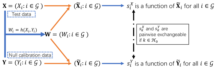
Figure 1: A graphical illustration of constructing the baseline data and calculating the scores. To create $\tilde{\mathbf{X}}_{i}$ and $\tilde{\mathbf{Y}}_{i}$, each $W_{i}$ in $\mathbf{W}$ is replaced by $X_{i}$ and $(Y_{i})$ in turn, for $i\in\mathcal{G}$, with the values in remaining nodes unchanged. The same function $s_{k}(\cdot)$ is used for computing $s_{k}^{X}$ and $s_{k}^{Y}$, ensuring that the two scores are pairwise exchangeable if $k\in\mathcal{H}_{0}$.

Suppose that a smaller value of $s_{i}^{X}$ indicates stronger evidence against the null hypothesis. Intuitively, the rejection of $H_{0,i}$ requires two pieces of evidence: firstly, $s_{i}^{X}$ must be sufficiently small, and secondly, $s_{i}^{X}$ should be smaller than its null counterpart $s_{i}^{Y}$. Therefore, we only select small $s_{i}^{X}$ from the candidate rejection set $\mathcal{G}^{r}=\{i\in\mathcal{G}:s_{i}^{X}<s_{i}^{Y}\}$. Consider a class of thresholding rules $\boldsymbol{\delta}=(\delta_{i}:i\in\mathcal{G})$, where $\delta_{i}\equiv 0$ for $i\notin\mathcal{G}^{r}$, and $\delta_{i}=\mathbb{I}(s_{i}^{X}\leq t)$ for $i\in\mathcal{G}^{r}$. Correspondingly, we introduce the concept of the mirror calibration set $\mathcal{G}^{c}=\{i\in\mathcal{G}:s_{i}^{Y}<s_{i}^{X}\}$. This mirror set of null scores $\{s_{i}^{Y}:i\in\mathcal{G}^{c}\}$ allows us to characterize the joint behavior of their counterparts $\{s_{i}^{X}:i\in\mathcal{G}^{r}\}$ under the null. It follows that the true FDP process and its mirror conservative process, denoted $Q(t)$, are respectively given by

$$\mbox{FDP}(t)=\frac{\sum_{j\in\mathcal{G}^{r}\cap\mathcal{H}_{0}}\mathbb{I}\left\{s_{j}^{X}\leq t\right\}}{(\sum_{j\in\mathcal{G}^{r}}\mathbb{I}\left\{s_{j}^{X}\leq t\right\})\vee 1},\quad Q(t)=\frac{1+\sum_{j\in\mathcal{G}^{c}}\mathbb{I}\left\{s_{j}^{Y}\leq t\right\}}{{(\sum_{j\in\mathcal{G}^{r}}\mathbb{I}\left\{s_{j}^{X}\leq t\right\})\vee 1}},\quad t>0.$$ (6)

To gain a better understanding of our methodology, it is helpful to note that $Q(t)$ provides a conservative estimate of $\mbox{FDP}(t)$. This conservativeness arises from two factors: (a) $\sum_{j\in\mathcal{G}^{c}}\mathbb{I}\{s_{j}^{Y}\leq t\}$ is always greater than or equal to $\sum_{j\in\mathcal{G}^{c}\cap\mathcal{H}_{0}}\mathbb{I}\{s_{j}^{Y}\leq t\}$; and (b) $\sum_{j\in\mathcal{G}^{c}\cap\mathcal{H}_{0}}\mathbb{I}\{s_{j}^{Y}\leq t\}$ can be seen as a mirror process that resembles the unobserved process $\sum_{j\in\mathcal{G}^{r}\cap\mathcal{H}_{0}}\mathbb{I}\{s_{j}^{X}\leq t\}$ since, as will be established in the next subsection (Property 3), $s_{j}^{X}$ and $s_{j}^{Y}$ are pairwise exchangeable under the null hypothesis. We choose the largest threshold, denoted as $\tau$, such that the conservative estimate of the FDP falls below the designated FDR level $\alpha$:

$$\tau=\sup\left\{t\in\mathbf{S}_{X}\cup\mathbf{S}_{Y}:Q(t)\leq\alpha\right\}.$$

The proposed PLIS procedure, summarized in Algorithm 1, rejects $H_{0,i}$ if $\delta_{i}\equiv\mathbb{I}(i\in\mathcal{G}^{r},s_{i}^{X}\leq\tau)=1$. By mathematical conventions, the supremum of an empty set is defined as $-\infty$. Therefore, if the set $\{t\in\mathbf{S}_{X}\cup\mathbf{S}_{Y}:Q(t)\leq\alpha\}$ is empty, then $\tau$ is set to $-\infty$, and Algorithm 1 does not reject any hypotheses.

Algorithm 1 The PLIS procedure

0:  The observations $\mathbf{X}=(X_{i}:i\in\mathcal{G})$ , the null distribution $F_{0}$, a pre-specified FDR level $\alpha$, a working model $\mathcal{M}$ and a computational algorithm $\mathcal{A}$.

0:  A decision rule $\boldsymbol{\delta}=(\delta_{i}:i\in\mathcal{G})$.

1:  Generate $\mathbf{Y}=(Y_{i}:i\in\mathcal{G})$, where $Y_{i}$ are i.i.d. observations from $F_{0}$.

2:  Create $\mathbf{W}=(W_{i}:i\in\mathcal{G})$, where $W_{i}=h(X_{i},Y_{i})$ and $h(x,y)$ is given by (5). Construct $\tilde{\mathbf{X}}_{i}$ and $\tilde{\mathbf{Y}}_{i}$ by respectively substituting $X_{i}$ and $Y_{i}$ in place of $W_{i}$ in $\mathbf{W}$ for $i\in\mathcal{G}$.

3:  Calculate $s_{i}^{X}\equiv{\mathbb{P}}_{\mathcal{M,A}}(\theta_{i}=0|\tilde{\mathbf{X}}_{i})$ and $s_{i}^{Y}\equiv{\mathbb{P}}_{\mathcal{M,A}}(\theta_{i}=0|\tilde{\mathbf{Y}}_{i})$ for $i\in\mathcal{G}$ with the user-specified working model $\mathcal{M}$ and algorithm $\mathcal{A}$. Let $\mathcal{G}^{r}=\{i:s_{i}^{X}<s_{i}^{Y}\}$.

4:  Let $\tau=\sup\{t\in\mathbf{S}_{X}\cup\mathbf{S}_{Y}:Q(t)\leq\alpha\}$, where $Q(t)$ is defined in (6).

5:  Let $\delta_{i}=\mathbb{I}\{s_{i}^{X}\leq\tau\}$ for $i\in\mathcal{G}^{r}$, otherwise $\delta_{i}=0$.

6:  Return $\boldsymbol{\delta}=(\delta_{i}:i\in\mathcal{G})$.

We conclude this subsection with several remarks. First, in order to ensure pairwise exchangeability between $s_{i}^{X}$ and $s_{i}^{Y}$ under the null, it is crucial to estimate the working model $\mathcal{M}$ from $\mathbf{W}$ before calculating the conformity scores. Detailed explanations and practical guidelines for the deployment of PLIS under two widely-used working models can be found in Section 2.5. Second, we can define an alternative estimate of $\mbox{FDP}(t)$, denoted as $Q^{\prime}(t)$, by substituting $\mathcal{G}$ in place of both $\mathcal{G}^{r}$ and $\mathcal{G}^{c}$ in equation (6). However, employing $Q^{\prime}(t)$ tends to be overly conservative. This conservativeness can be effectively mitigated by our $Q(t)$ that confines the rejections within $\mathcal{G}^{r}$; further elaborations on this are provided in Sections 3.3 and 4.3. Finally, the decision process of Algorithm 1 closely resembles that of the BH algorithm with conformal $p$-values, although it incorporates several modifications. Related discussions are provided in Section D of the Supplement.

2.4 Theory

We start by establishing several exchangeability properties, first for the data points and subsequently for the conformity scores. The random elements $\{Z_{i}:i\in[K]\}$ are said to be (jointly) exchangeable if the distribution of $(Z_{1},\cdots,Z_{K})$ is the same as that of $(Z_{\tau_{1}},\cdots,Z_{\tau_{K}})$ for any permutation $(\tau_{1},\cdots,\tau_{K})$ of the indices $\{1,\cdots,K\}$. We write $(Z_{1},\cdots,Z_{K})\overset{d}{=}(Z_{\tau_{1}},\cdots,Z_{\tau_{K}}),$ where $\overset{d}{=}$ denotes equality in distribution. We will soon introduce a weaker notion, the pairwise exchangeability, which is more relevant to our theory. The following exchangeability properties are proven in Appendix A.

The first property can be easily deduced from the definition of Model (2) and the construction of $\mathbf{W}$ outlined in Algorithm 1.

Property 1 (Exchangeability and conditional independence between data points).

Suppose $\mathbf{X}=(X_{i}:i\in\mathcal{G})$ are observations from Model (2), and $(Y_{i}:i\in\mathcal{G})$ are randomly drawn from the null distribution $F_{0}$. Then we have: (a) The random variables $\left\{Y_{i},i\in\mathcal{G};X_{j},j\in\mathcal{H}_{0}\right\}$ are jointly exchangeable; (b) $\{Z_{j}=\{X_{j},Y_{j}\}:j\in\mathcal{G}\}$ are conditionally independent given $\mathbf{W}$ and $\boldsymbol{\Theta}$; (c) For $i\in\mathcal{H}_{0}$, $X_{i}$ and $Y_{i}$ are pairwise exchangeable conditional on $\mathbf{W}$ and $\boldsymbol{\Theta}$, i.e., $(X_{i},Y_{i}|\mathbf{W},\boldsymbol{\Theta})\overset{d}{=}(Y_{i},X_{i}|\mathbf{W},\boldsymbol{\Theta}).$

The next property characterizes the pairwise exchangeability between $\tilde{\mathbf{X}}_{j}$ and $\tilde{\mathbf{Y}}_{j}$.

Property 2 (Pairwise exchangeability and conditional independence between data sets).

Consider $\tilde{\mathbf{X}}_{j}$ and $\tilde{\mathbf{Y}}_{j}$ as generated according to Algorithm 1. Then we have: (a) $\{\mathcal{D}_{j}=\{\tilde{\mathbf{X}}_{j},\tilde{\mathbf{Y}}_{j}\}:j\in\mathcal{G}\}$ are conditionally independent given $\mathbf{W}$ and $\boldsymbol{\Theta}$; (b) For $i\in\mathcal{H}_{0}$, $\tilde{\mathbf{X}}_{i}$ and $\tilde{\mathbf{Y}}_{i}$ are pairwise exchangeable, i.e. $(\tilde{\mathbf{X}}_{i},\tilde{\mathbf{Y}}_{i}|\mathbf{W},\boldsymbol{\Theta})\overset{d}{=}(\tilde{\mathbf{Y}}_{i},\tilde{\mathbf{X}}_{i}|\mathbf{W},\boldsymbol{\Theta})$.

The next property is concerned with the conditional independence and pairwise exchangeability between null scores.

Property 3 (Pairwise exchangeability and conditional independence between scores).

Consider scores $s_{j}^{X}$ and $s_{j}^{Y}$ computed according to Algorithm 1, denote $\mathbf{s}_{j}=\{s_{j}^{X},s_{j}^{Y}\}$ for $j\in\mathcal{G}$. Then we have: (a) $\{\mathbf{s}_{j}:j\in\mathcal{G}\}$ are conditionally independent given $\mathbf{W}$ and $\boldsymbol{\Theta}$; (b) Denote $\mathbf{S}_{-i}=\cup_{j\in\mathcal{G},j\neq i}\mathbf{s}_{j}$. For $i\in\mathcal{H}_{0}$, $s_{i}^{X}$ and $s_{i}^{Y}$ are pairwise exchangeable given $\mathbf{S}_{-i}$:

$$(s_{i}^{X},s_{i}^{Y}|\mathbf{S}_{-i})\overset{d}{=}(s_{i}^{Y},s_{i}^{X}|\mathbf{S}_{-i}),\text{ or equivalently }(s_{i}^{X},s_{i}^{Y},\mathbf{S}_{-i})\overset{d}{=}(s_{i}^{Y},s_{i}^{X},\mathbf{S}_{-i}).$$ (7)

The pairwise exchangeability (7), which is crucial in proving the FDR theory for PLIS, is a weaker assumption than the joint exchangeability among all null scores $\{s_{i}^{X}:i\in\mathcal{H}_{0}\}\cup\{s_{i}^{Y}:i\in\mathcal{G}\}$ required in most existing literature of conformal inference. Now we state our main theorem that establishes the validity of PLIS for controlling the FDR.

Theorem 1.

Consider Model (2) and the PLIS procedure outlined in Algorithm 1. Then Properties 1-3 hold and PLIS controls the FDR at level $\alpha$.

Our approach distinguishes itself from existing theories in conformal inference that depend on joint exchangeability, which is necessary either for creating super-martingales (Yang et al., 2021; Mary and Roquain, 2022) or for establishing PRDS properties (Marandon et al., 2022; Bates et al., 2023). Instead, we present a framework that leverages only the pairwise exchangeability.

2.5 Practical guidelines and examples

PLIS utilizes resampling techniques to generate a mirror process that quantifies the FDP in multiple testing. At its core, PLIS can be situated within the conformal inference framework, which facilitates the development of valid FDR rules that exhibit enhanced robustness to model misspecification. This section presents examples that contextualize PLIS as a valuable tool for “conformalizing” some well-known FDR procedures, producing inferences that possess similar operational characteristics as state-of-the-art conformal methods (Yang et al., 2021; Marandon et al., 2022; Liang et al., 2022; Bates et al., 2023).

Example 1. Conformalizing the LIS procedure under HMMs.

A variety of real-world applications involve data with HMM-type structures. Several works (Sun and Cai, 2009; Perrot-Dockès et al., 2021) have demonstrated that exploiting the HMM structure can greatly enhance the power of FDR analysis. However, their theoretical analysis necessitates certain conditions to be satisfied, such as homogeneous transition probabilities and identical non-null distributions, which may not be strictly met in practical scenarios. The HMMs are characterized by a set of parameters, denoted as ${\vartheta}=(\mathbf{A},f_{0},f_{1})$, where $\mathbf{A}$ is the transition probability matrix, and $f_{0}$ and $f_{1}$ are the emission densities for the null and non-null observations, respectively.

In our setup, we use $\mathcal{M}_{\rm HM}$ as the HMM working model, where $\vartheta$ is estimated using the EM algorithm on $\mathbf{W}$. To implement the PLIS procedure, we utilize the forward-backward algorithm, denoted by $\mathcal{A}_{\rm FB}$, to compute the scores $s_{i}^{X}=\mathbb{P}_{\mathcal{M}_{\rm HM},\mathcal{A}_{\rm FB}}(\theta_{i}=0|\tilde{\mathbf{X}}_{i})$ and $s_{i}^{Y}=\mathbb{P}_{\mathcal{M}_{\rm HM},\mathcal{A}_{\rm FB}}(\theta_{i}=0|\tilde{\mathbf{Y}}_{i})$ for $i\in\mathcal{G}$. The decision-making process is based on Algorithm 1. The PLIS procedure can be regarded as a conformalized adaptation of the LIS procedure proposed by Sun and Cai (2009), computed using $\mathcal{M}_{\rm HM}$ and algorithm $\mathcal{A}_{\rm FB}$. PLIS differs from LIS in that it can handle a variety of data structures that deviate from HMMs. This ability ensures valid FDR control in finite-samples, even when the working model is misspecified or the model parameters are estimated poorly. ∎

Example 2. Conformalizing the adaptive $z$-value procedure under the two-group model (3) with independent observations.

In the context where observations are assumed to be independent and Efron’s two-group model (3), denoted $\mathcal{M}_{\rm TG}$, is adopted, Sun and Cai (2007) showed that the density ratio (DR) $r(x)=\frac{f_{0}(x)}{{f}(x)}$ or the local false discovery rate ${\mathrm{Lfdr}}(x)=(1-\pi)r(x)$ serves as the optimal building block for FDR analysis. The PLIS framework treats DR and Lfdr equivalently since $(1-\pi)$ is a constant across all study units and only the relative ranking contributes to the operation of PLIS. Using the working model $\mathcal{M}_{\rm TG}$, the conformity score $s_{i}(\cdot)$ can be taken as the DR function $\hat{r}(\cdot)=f_{0}(\cdot)/\hat{f}(\cdot)$, where $f_{0}$ is known, and $\hat{f}(\cdot)$ is the standard kernel density estimator constructed based on $\mathbf{W}$. The PLIS procedure operates by employing $s_{i}^{X}\equiv\hat{r}(X_{i})$ and $s_{i}^{Y}\equiv\hat{r}(Y_{i})$ in Algorithm 1. As carefully explained in Section D.6 of the Supplement, although DR is permutation-invariant with respect to $\mathbf{W}$, the null scores are not jointly exchangeable. By contrast, PLIS still works since $(s_{i}^{X},s_{i}^{Y})$ are pairwise exchangeable given $\mathbf{W}$ and $\boldsymbol{\Theta}$.

Sun and Cai (2007) proposed a class of adaptive $z$-value (AZ) procedures, and showed that AZ outperforms $p$-value based methods by adapting to the shape of the alternative distribution. PLIS may be viewed as a conformalized adaptation of AZ, which effectively incorporates the structural information into inference while controlling the FDR in finite samples. This represents a notable advantage over the AZ procedure, which only ensures asymptotic FDR control. ∎

Our customized PLIS procedures remain valid as long as the underlying model belongs to the broad class (2), regardless of the working models or algorithms used. Constructing conformity scores through suitable working models and efficient algorithms is crucial for enhancing the power of PLIS. Furthermore, the recently proposed AdaDetect method (Marandon et al., 2022) shares similar advantages with PLIS under the two-group model. However, in situations where asymmetric rules are most effective for addressing the problem at hand, PLIS significantly diverges from AdaDetect.

2.6 Semi-supervised PLIS

This section considers the scenario where users only have access to $n$ labeled null data points $\mathbf{U}=\{U_{1},\cdots,U_{n}\}$ and aim to predict the labels of $m$ new data points $\{X_{i}:i\in\mathcal{G}\}$, with $n>m$. This scenario is known as the semi-supervised multiple testing problem (Mary and Roquain, 2022) and is closely related to outlier detection in the conformal inference literature (Marandon et al., 2022; Bates et al., 2023). Semi-supervised multiple testing, which leverages labeled null data without prior knowledge of the null distribution, differs from conventional multiple testing that possesses knowledge of the null distribution. We introduce a semi-supervised PLIS (Algorithm 2) to handle this novel scenario.

The algorithm first partitions the labeled null data $\mathbf{U}$ into two subsets: the calibration set $\mathbf{Y}=(Y_{i}:i\in\mathcal{G})$ and the training set $\mathbf{U}^{tr}=\mathbf{U}\setminus\mathbf{Y}$. The test data $\mathbf{X}$ and calibration data $\mathbf{Y}$ are then utilized to construct the baseline data $\mathbf{W}$ by following the same steps in Algorithm 1. We move on to the estimation issue. In the case of an HMM, an estimator for the emission distribution $f_{0}$ can be learned from the labeled null data $\mathbf{U}^{tr}$. Subsequently, we utilize the baseline data $\mathbf{W}$ to estimate $f_{1}$ and transition probabilities via the EM algorithm, and then calculate the conformity scores via the forward-backward procedure. If the working model is a two-group model, the conformity scores correspond to the density ratios, which can be estimated using both $\mathbf{U}^{tr}$ and $\mathbf{W}$ via the positive unlabeled (PU) learning algorithms. This approach has also been suggested by Marandon et al. (2022). See Algorithm 2 for a concise summary of the steps involved.

Algorithm 2 The semi-supervised PLIS procedure

0:  The test data $\mathbf{X}=(X_{i}:i\in\mathcal{G})$ , the null samples $\mathbf{U}=\{U_{1},\cdots,U_{n}\}$, a pre-specified FDR level $\alpha$, a working model $\mathcal{M}$ and a computational algorithm $\mathcal{A}$.

0:  A decision rule $\boldsymbol{\delta}=(\delta_{i}:i\in\mathcal{G})$.

1:  Split $\mathbf{U}$ into the calibration data $\mathbf{Y}=(Y_{i}:i\in\mathcal{G})$ and the training data $\mathbf{U}^{tr}=\mathbf{Z}\setminus\mathbf{Y}$

2:  Create $\mathbf{W}=(W_{i}:i\in\mathcal{G})$, where $W_{i}=h(X_{i},Y_{i})$ and $h(x,y)$ is given by (5). Construct $\tilde{\mathbf{X}}_{i}$ and $\tilde{\mathbf{Y}}_{i}$ by respectively substituting $X_{i}$ and $Y_{i}$ in place of $W_{i}$ in $\mathbf{W}$ for $i\in\mathcal{G}$.

3:  Calculate $s_{i}^{X}\equiv{\mathbb{P}}_{\mathcal{M,A}}(\theta_{i}=0|\tilde{\mathbf{X}}_{i})$ and $s_{i}^{Y}\equiv{\mathbb{P}}_{\mathcal{M,A}}(\theta_{i}=0|\tilde{\mathbf{Y}}_{i})$ for $i\in\mathcal{G}$ with the user-specified working model $\mathcal{M}$ and algorithm $\mathcal{A}$ based on $\mathbf{W}$ and $\mathbf{U}^{tr}$.

4:  Let $\tau=\sup\{t\in\mathbf{S}_{X}\cup\mathbf{S}_{Y}:Q(t)\leq\alpha\}$, where $Q(t)$ is defined in (6).

5:  Let $\delta_{i}=\mathbb{I}\{s_{i}^{X}\leq\tau\}$ for $i\in\mathcal{G}^{r}=\{j\in\mathcal{G}:s_{j}^{X}<s_{j}^{Y}\}$, otherwise $\delta_{i}=0$.

6:  Return $\boldsymbol{\delta}=(\delta_{i}:i\in\mathcal{G})$.

Remark 2.

Here we have assigned exactly one null data point to each test unit, but in situations where there is an abundance of null samples, it may be appropriate to employ the de-randomization idea in Section 3.2 to improve stability. In situations where the calibration dataset is smaller than $m$, one may conduct an independent screening procedure to narrow down the focus before using PLIS on a smaller subset of hypotheses. These represent interesting issues for future investigation.

The next theorem, established using de Finetti’s theorem (cf. Section C in the Supplement) and techniques employed in proving Properties 1-3, generalizes Theorem 1 in two ways. Firstly, it considers the setup of semi-supervised multiple testing, where we have access to labeled null data instead of explicit knowledge of the null distribution. Secondly, it relaxes the assumption of conditional independence given $\boldsymbol{\Theta}$ in Model (2) by allowing for correlated noise in the data generation process.

Theorem 2.

Consider Algorithm 2, if the null data $\{U_{1},\cdots,U_{n},X_{i},i\in\mathcal{H}_{0}\}$ are exchangeable conditional on the non-null data $\{X_{i}:i\notin\mathcal{H}_{0}\}$, then (a) for $i\in\mathcal{H}_{0}$, $s_{i}^{X}$ and $s_{i}^{Y}$ are pairwise exchangeable given $\mathbf{S}_{-i}$; and (b) Algorithm 2 controls FDR at $\alpha$.

In Section E.4 of the Supplement, we provide numerical results to corroborate Theorem 2 by considering the semi-supervised setup in which correlated noises are introduced to the observations generated from Model (2).

2.7 Conformal $q$-values

When the joint exchangeability condition fails to hold, conformal $p$-values can no longer be properly defined. To address this issue, we introduce the concept of conformal $q$-value as a significance index to measure the risk associated with individual decisions.

We begin by examining $Q(t)$ in (6), which offers a conservative estimate of the FDP. Consider the minimum FDR level $\alpha$ at which $H_{0,i}$ can be “just” rejected:

$$q_{i}\equiv\min_{t\in\mathbf{S}_{X}\cup\mathbf{S}_{Y},t\geq s_{i}^{X}}Q(t),\text{ for }i\in\mathcal{G}^{r};\quad q_{i}\equiv 1,\text{ for }i\in\mathcal{G}\setminus\mathcal{G}^{r}.$$ (8)

The adjusted $q_{i}$ is referred to as the conformal $q$-value corresponding to $H_{0,i}$, owing to its resemblance to the $q$-value idea introduced by Storey (2003). While Storey’s $q$-value is constructed based on the empirical distribution of $p$-values, our conformal $q$-value is derived from a resampling method and a carefully designed mirror process.

The conformal $q$-value is a valid and user-friendly significance index that provides clear interpretability for individual decisions, and practitioners can directly use it for decision-making by comparing them with a pre-specified $\alpha$. Theorem 1 and the Proposition below establish the validity of using the conformal $q$-value (8) in FDR analysis.

Proposition 1.

Consider the PLIS procedure as outlined in Algorithm 1 and the conformal $q$-value defined by equation (8). Then the decision $\delta_{i}$ presented in Algorithm 1 is equivalent to rejecting $H_{0,i}$ if $q_{i}\leq\alpha$.

3 Connections to Existing Works and Extensions

In this section, we first establish the connection between PLIS and the e-BH method (Section 3.1), then introduce several ensuing extensions: derandomized PLIS (Section 3.2), as well as ${\rm PLIS}_{\rm cbh}$ and ${\rm PLIS}_{\rm sym}$ (Sections 3.3). Finally, we discuss the distinctions of PLIS from related works (Section 3.4).

3.1 Connection to the e-BH procedure

In hypothesis testing, an e-value (Vovk and Wang, 2021) is defined as the observed value of a non-negative random variable $E$ that satisfies the condition $\mathbb{E}[E]\leq 1$ under the null hypothesis. E-values can be constructed using betting scores (Shafer, 2021), likelihood ratios, and stopped super-martingales (Grünwald et al., 2020). This section demonstrates how the PLIS framework can be utilized to construct robust and powerful e-values.

Let $(e_{i}:1\leq i\leq m)$ be the e-values for testing $(H_{0,i}:1\leq i\leq m)$. Wang and Ramdas (2022) proposed the e-BH procedure, which involves first ordering the e-values as $e_{(1)}\geq e_{(2)}\geq\cdots\geq e_{(m)}$, and then choosing a cutoff along the ranking using the following step-wise algorithm. Let $\hat{k}=\max\left\{i:(i/m)e_{(i)}\geq(1/\alpha)\right\}$, then reject hypotheses in the set $\mathcal{R}_{ebh}=\{1\leq j\leq m:e_{j}\geq e_{(\hat{k})}\}$. We call $\{e_{j}:1\leq j\leq m\}$ a set of generalized e-values if

$$\mathbb{E}\left(\textstyle\sum_{j\in\mathcal{H}_{0}}e_{j}\right)\leq m.$$ (9)

Condition (9) is strictly weaker than the condition that $\mathbb{E}[e_{j}]\leq 1$ for all $j\in\mathcal{H}_{0}$. Wang and Ramdas (2022) proved that if $\{e_{j}:1\leq j\leq m\}$ are a set of generalized e-values, then the e-BH procedure controls FDR at $\alpha$ under arbitrary dependence. We can construct a set of generalized e-values based on the PLIS framework. Specifically, define

$$e_{j}=\frac{m\delta_{j}}{1+\sum_{i\in\mathcal{G}^{c}}\mathbb{I}\{s_{i}^{Y}\leq\tau\}},\quad\mbox{for $j\in\mathcal{G}$},$$ (10)

where $\delta_{j}$, $\mathcal{G}^{c}$ and $\tau$ are defined by Algorithm 1. The following theorem can be proved using similar techniques for proving Theorem 1.

Theorem 3.

The variables $e_{j}$ defined in (10) constitute a set of generalized e-values.

The following proposition demonstrates that the PLIS procedure is equivalent to implementing the e-BH procedure with generalized e-values as defined by (10). The connection to e-BH offers valuable insights into our theory, providing a new perspective on why PLIS performs robustly in the face of general dependence and model misspecification.

Proposition 2.

If we implement the e-BH procedure with e-values in (10), then the rejection set $\mathcal{R}_{ebh}=\mathcal{R}$, where $\mathcal{R}=\{i\in\mathcal{G}:\delta_{i}=1\}$ is the set of rejected hypotheses by Algorithm 1.

3.2 Derandomized PLIS

While the PLIS framework employs resampling methods, which can introduce additional uncertainties and may be viewed as undesirable by practitioners, the fact that the average of e-values is still an e-value (Vovk and Wang, 2021) offers motivation to consider a principled derandomization method. This involves aggregating multiple random samples to reduce variability. Similar ideas have been utilized in contemporaneous works, including Ren and Barber (2023) and Bashari et al. (2023).

The derandomized PLIS procedure involves running the PLIS procedure repeatedly for $N$ times and averaging the results for decision-making. Specifically, for the $k$-th replication, $k\in[N]$, we generate $\{Y_{j}^{(k)}:j\in\mathcal{G}\}\overset{i.i.d.}{\sim}f_{0}$, and construct $\tilde{\mathbf{X}}_{i}^{(k)}$ and $\tilde{\mathbf{Y}}_{i}^{(k)}$ by respectively substituting $X_{i}^{(k)}$ and $Y_{i}^{(k)}$ in place of $W_{i}^{(k)}$ in $\mathbf{W}^{(k)}$, where $\mathbf{W}^{(k)}$ is created by combining $\mathbf{X}$ and $\mathbf{Y}^{(k)}=(Y_{i}^{(k)}:i\in\mathcal{G})$ via (5). We then compute the scores $\{s_{i}^{X(k)},s_{i}^{Y(k)}:i\in\mathcal{G}\}$ and threshold $\tau^{(k)}$ based on Algorithm 1. The corresponding e-values $\{e_{i}^{(k)}:i\in\mathcal{G}\}$ for replication $k$ can be calculated using (10). This process is repeated for $k=1,\cdots,N$. Finally, we average the individual e-values $e_{i}^{(k)}$ to compute the summary e-values $\bar{e}_{i}=\frac{1}{N}\sum_{k=1}^{N}e_{i}^{(k)}$ for all $i\in\mathcal{G}$, and apply the e-BH procedure with $\{\bar{e}_{i}:i\in\mathcal{G}\}$. The proposed derandomized PLIS procedure is summarized in Algorithm 3. The theoretical guarantee of derandomized PLIS for FDR control follows directly from the validity of the e-BH procedure and Proposition 2.

Remark 3.

Algorithm 3 has allowed different replications to have varied $(\alpha_{k})_{k=1}^{N}$. As noted by Ren and Barber (2023), derandomization could lead to higher power if the e-values are carefully aggregated through powerful weighting schemes. We have investigated this issue with some preliminary results provided in Section E.6 in the Supplement. The development of optimal weights is an interesting direction for future research.

Algorithm 3 The Derandomized PLIS procedure

0:  Observations $\mathbf{X}=(X_{i}:i\in\mathcal{G})$, the null distribution $F_{0}$, working model $\mathcal{M}$, algorithm $\mathcal{A}$, number of replications $N$, weights $(\alpha_{k})_{k=1}^{N}$, nominal FDR level $\alpha$.

0:  Decisions $\boldsymbol{\delta}=(\delta_{i}:i\in\mathcal{G})$.

1:  for all $k=1,2,\cdots,N$ do

2:     Generate $\{Y_{j}^{(k)}\}_{j=1}^{m}\overset{i.i.d.}{\sim}F_{0}$. Denote $\mathbf{Y}^{(k)}=(Y_{j}^{(k)}:j\in\mathcal{G})$.

3:     Create $\mathbf{W}^{(k)}=(W_{i}^{(k)}:i\in\mathcal{G})$ by combining $\mathbf{X}$ and $\mathbf{Y}^{(k)}$ via (5). Construct $\tilde{\mathbf{X}}_{i}^{(k)}$ and $\tilde{\mathbf{Y}}_{i}^{(k)}$ by respectively substituting $X_{i}$ and $Y_{i}^{(k)}$ in place of $W_{i}^{(k)}$ in $\mathbf{W}^{(k)}$ for $i\in\mathcal{G}$.

4:     Calculate $s_{i}^{X(k)}\equiv{\mathbb{P}}_{\mathcal{M,A}}(\theta_{i}=0|\tilde{\mathbf{X}}_{i}^{(k)})$ and $s_{i}^{Y(k)}\equiv{\mathbb{P}}_{\mathcal{M,A}}(\theta_{i}=0|\tilde{\mathbf{Y}}_{i}^{(k)})$ for $i\in\mathcal{G}$ with user-specified working model $\mathcal{M}$ and algorithm $\mathcal{A}$. Let $\mathcal{G}^{r(k)}=\{i\in\mathcal{G}:s_{i}^{X(k)}<s_{i}^{Y(k)}\}$, $\mathcal{G}^{c(k)}=\{i\in\mathcal{G}:s_{i}^{Y(k)}<s_{i}^{X(k)}\}$, and $\mathbf{S}_{X}^{(k)}=\{s_{i}^{X(k)}\}_{i\in\mathcal{G}}$, $\mathbf{S}_{Y}^{(k)}=\{s_{i}^{Y(k)}\}_{i\in\mathcal{G}}$.

5:     Let $Q^{(k)}(t)=\frac{1+\sum_{i\in\mathcal{G}^{c(k)}}\mathbb{I}\{s_{i}^{Y(k)}\leq t\}}{1\vee(\sum_{i\in\mathcal{G}^{r(k)}}\mathbb{I}\{s_{i}^{X(k)}\leq t\})}$ and $\tau^{(k)}=\sup\{t\in\mathbf{S}_{X}^{(k)}\cup\mathbf{S}_{Y}^{(k)}:Q^{(k)}(t)\leq\alpha_{k}\}$.

6:     Calculate $e_{i}^{(k)}=\frac{m\mathbb{I}\{s_{i}^{X(k)}\leq\tau^{(k)}\}}{1+\sum_{j\in\mathcal{G}^{c(k)}}\mathbb{I}\{s_{j}^{Y(k)}\leq\tau^{(k)}\}}$ for $i\in\mathcal{G}^{r(k)}$, otherwise $e_{i}^{(k)}=0$.

7:  end for

8:  Let $\bar{e}_{i}=\frac{1}{N}\sum_{k=1}^{N}e_{i}^{(k)}$ for $i\in\mathcal{G}$. Denote the ordered statistics by $\bar{e}_{(1)}\geq\bar{e}_{(2)}\geq\cdots\geq\bar{e}_{(m)}$. Let $\hat{k}=\max\{i:({i\bar{e}_{(i)}}/{m})\geq({1}/{\alpha})\}$.

9:  Let $\delta_{i}=\mathbb{I}\{\bar{e}_{i}\geq\bar{e}_{(\hat{k})}\}$ for $i\in\mathcal{G}$. Return $\boldsymbol{\delta}=(\delta_{i}:i\in\mathcal{G})$

3.3 Comparison with conformal and knockoff methods

PLIS is developed based on the principles of conformal inference, which involves the utilization of machine learning algorithms to calculate conformity scores and the employment of calibration data to quantify the uncertainties in the decision-making process. We have implemented several enhancements that effectively address the limitations commonly associated with conformal inference methods. These enhancements include the novel construction of baseline data $\mathbf{W}$, the development of pairwise exchangeable scores, and the refinement with the candidate rejection set $\mathcal{G}^{r}$. This section discusses two variations of PLIS, highlighting its connection to existing works and providing insights on its merits.

The first variation, denoted as ${\rm PLIS}_{\rm cbh}$, is based on an insightful connection between the conformal BH procedure and the knockoff method (Mary and Roquain, 2022). This connection demonstrates that applying BH with conformal $p$-values is equivalent to utilizing the counting knockoff technique for i.i.d. design (Weinstein et al., 2017). However, implementing the counting knockoff technique with the pairwise exchangeable scores generated by Algorithm 1 yields excessively conservative FDR procedures (cf. Section 4.3). Furthermore, it is inappropriate to employ the adaptive BH procedure (Weinstein et al., 2017; Marandon et al., 2022; Bates et al., 2023) as a way of mitigating this conservativeness, as pairwise exchangeable scores produce invalid conformal $p$-values that lack super-uniformity, and fail to fulfill the PRDS condition.

The second variation, denoted as ${\rm PLIS}_{\rm sym}$, incorporates a symmetrization step through constructing contrasts between pairs of scores. This strategy, inspired by the idea in Barber and Candès (2015), employs anti-symmetric functions that satisfy $T_{j}(a,b)=-T_{j}(b,a)$ to convert pairwise exchangeable scores into symmetrized test statistics. Symmetrization techniques have been successfully applied in regression settings (Candès et al., 2018; Ren and Candès, 2023; Du et al., 2023). Let $T_{j}\equiv s_{j}^{Y}-s_{j}^{X}$, where $s_{j}^{X}$ and $s_{j}^{X}$ are pairwise exchangeable scores generated by Algorithm 1. A larger value of $T_{j}$ indicates stronger evidence against $H_{0,j}$. Using arguments in Barber and Candès (2015), we can show that Property 3 guarantees that all null $T_{j}$ satisfy the flip-sign condition, i.e. $\{\mathrm{sign}(T_{j}):j\in\mathcal{H}_{0}\}$ are i.i.d. coin flips conditional on $\{|T_{j}|:j\in\mathcal{G}\}$. We reject $H_{0,j}$ if $T_{j}\geq\tau_{\rm sym}$, where $\tau_{\rm sym}$ is determined by the following mirror process:

$$\tau_{\rm sym}=\inf\left\{t\in\{|T_{j}|:j\in\mathcal{G}\}:\frac{1+\sum_{j\in\mathcal{G}}\mathbb{I}\{T_{j}\leq-t\}}{\sum_{j\in\mathcal{G}}\mathbb{I}\{T_{j}\geq t\}}\leq\alpha\right\}.$$

However, utilizing $T_{j}=s_{j}^{Y}-s_{j}^{X}$ may lead to severe loss of valuable structural information. This is because the contrast $s_{j}^{Y}-s_{j}^{X}$ has a tendency to cancel out the clustering structure inherent among non-null effects. The rankings generated by $T_{j}$ are generally inferior when compared to the rankings generated by $s_{j}^{X}$.

Section 4.3 presents numerical results that illustrate the advantages of PLIS over ${\rm PLIS}_{\rm cbh}$ and ${\rm PLIS}_{\rm sym}$. We refer to Section D of the Supplement for more in-depth discussion.

3.4 Comparison with covariate-adaptive methods

Structured multiple testing is a subject of extensive research that has attracted significant interest. Our PLIS procedure distinguishes itself from existing covariate-adaptive methods in several aspects. Firstly, in the works of Lei and Fithian (2018), Ignatiadis and Huber (2021) and Ren and Candès (2023), the structural information is represented by a covariate sequence and is incorporated through techniques such as weighted $p$-values or covariate-adaptive thresholds. By contrast, our approach leverages structural knowledge about the underlying data generation process and integrates it into inference via a user-specified working model. Secondly, the theory in existing methods is developed based on group-wise cross-weighting (Ignatiadis and Huber, 2021) or covariate modulation through data masking (Lei and Fithian, 2018; Ren and Candès, 2023). In contrast, PLIS operates within the theoretical framework of conformal inference, harnessing the flexibility of machine learning algorithms to learn powerful conformity scores, with associated decision risk being assessed by employing carefully calibrated null scores. Thus, PLIS not only facilitates the effective incorporation of structural information but also guarantees the validity of inference, even in scenarios where the machine learning models are mis-specified. Finally, PLIS offers an intuitive, fast, and user-friendly computational algorithm that efficiently computes scores from the baseline data. This differs from the more computationally intensive algorithms proposed in Lei and Fithian (2018) and Ren and Candès (2023), which involve intricate techniques such as adaptive unmasking and boundary updating.

4 Simulation

This section presents simulation results that compare PLIS, which is implemented as described in the first example of Section 2.5, with several competing methods. For all of the numerical experiments, we set $m=2000$ and $\alpha=0.05$. The observations are generated following this model: $X_{i}|\theta_{i}\overset{ind.}{\sim}(1-\theta_{i})\mathcal{N}(0,1)+\theta_{i}\mathcal{N}(\mu,1)$. The latent states $\Theta$ obey various dependence structures in different experiments, which will be described in detail later. The following methods are considered in our analysis: (a) $\rm PLIS_{HM}$, implemented via Algorithm 1, utilizing the working model $\mathcal{M}_{\rm HM}$ as described in Section 2.5; (b) BH (Benjamini and Hochberg, 1995); (c) AdaDetect (Marandon et al., 2022), where the density ratio is estimated by $\hat{r}(\cdot)=f_{0}(\cdot)/\hat{f}(\cdot)$, with $f_{0}$ being known and $\hat{f}(\cdot)$ being the standard kernel estimator based on $\{\mathbf{X},\mathbf{Y}\}$. (d) $\rm PLIS_{TG}$, implemented via Algorithm 1 using the working model $\mathcal{M}_{\rm TG}$ as described in Section 2.5. (e) AdaPT (Lei and Fithian, 2018), implemented using the R package adaptMT. Throughout all the simulations conducted, the FDR and Average Power (AP) levels are computed by averaging the results obtained from 200 replications.

4.1 Comparisons with symmetric rules

We first consider HMMs in which $\boldsymbol{\Theta}=(\theta_{i})_{i=1}^{m}$ is a binary Markov chain with transition matrix $\mathbf{A}=(a_{ij})_{i,j=0,1}=\left(\mathbb{P}(\theta_{t+1}=j|\theta_{t}=i)\right)_{i,j=0,1}$. Here, we fix $a_{00}=0.95$, and the initial state of the latent chain is set to be $\theta_{1}=0$.

We apply BH, AdaDetect, AdaPT, $\rm PLIS_{HM}$ and $\rm PLIS_{TG}$ to the simulated data, and summarize the results in Figure 2. Our results demonstrate that all of the methods under consideration effectively control the FDR at the nominal level. Both the $\rm PLIS_{TG}$ and AdaDetect exhibit similar performance and outperform BH in terms of power. Notably, $\rm PLIS_{HM}$ demonstrates a conservative behavior, with the degree of conservativeness increasing as $a_{11}$ becomes larger. Despite this behavior, $\rm PLIS_{HM}$ exhibits the highest power among all five methods in most scenarios. This can be attributed to the use of asymmetric rules in $\rm PLIS_{HM}$. AdaPT outperforms/underperforms BH when $a_{11}$ becomes large/small. Additional simulation results for HMMs are presented in Section E.2 of the Supplement.

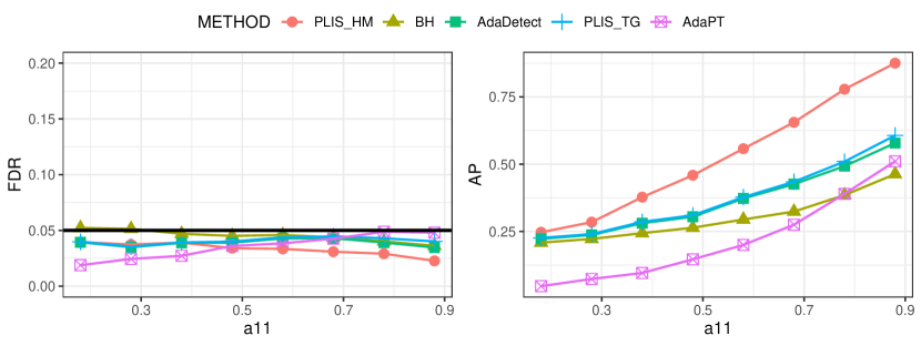
Figure 2: The comparison of FDR and AP for HMMs with $\mu=2.6$ and varying $a_{11}$.

4.2 Comparisons beyond HMMs

This section examines the case where the true transition matrices change over time, which is commonly referred to as a heterogeneous HMM. Such models are particularly useful since the structure of real-world data is often non-stationary. Specifically, we define $\mathbf{A}^{(k)}=\left(a_{ij}^{(k)}\right)_{i,j=0,1}$ as the transition probability matrix for the $k$-th transition, where $a_{ij}^{(k)}=\mathbb{P}(\theta_{k}=j|\theta_{k-1}=i)$, and $a_{00}^{(k)}=0.95$ is fixed for all $k$. The conditional distributions $F_{0}$ and $F_{1}$ remain the same as in the preceding simulations.

We consider a scenario in which $a_{11}^{(k)}=0.9e^{-k/1000}$ decreases with $k$ exponentially. This decreasing trend indicates that the stochastic system will gradually stabilize over time, with outliers becoming increasingly rare within the clusters. Although the data in this scenario possess a complex structure, accurately modeling them can be challenging. However, these data do exhibit patterns resembling HMMs, with moderate deviations from homogeneity conditions. Hence, we adopt a homogeneous HMM as a working model to capture the underlying structural patterns in the data and subsequently utilize the PLIS framework for inference. To assess the performance of PLIS and to compare it with other methods, specifically BH, AdaDetect, and AdaPT, we vary the parameter $\mu$ from 2 to 3 and apply these methods to simulated data. The results are summarized in Figure 3.

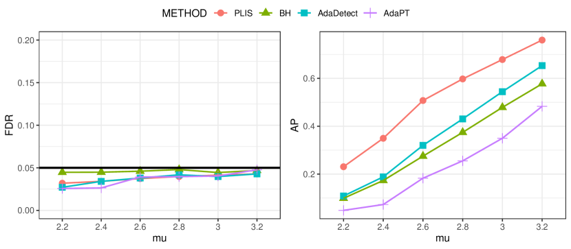
Figure 3: FDR and AP comparison for the heterogeneous HMM with exponentially vanishing $a_{11}$. Here $a_{11}^{(k)}=0.9e^{-k/1000}$.

Our results demonstrate that all methods are effective in controlling the FDR, with PLIS exhibiting higher average power and relatively lower FDR compared to other methods. This highlights the effectiveness of PLIS in leveraging structural information, even when wrong models and algorithms are employed. Similar trends are observed in the case of heterogeneous HMMs with periodic transition probabilities, as shown in Figure 8 in Section E of the Supplement. Additionally, our analysis of more general data structures, such as two-layer dynamic models and structured models generated from a renewal process, demonstrates that PLIS remains more powerful than the other methods, as depicted in Figure 9-10 in Section E of the Supplement. These findings underscore the versatility and robustness of PLIS in a variety of settings, and suggest that it has considerable potential for analyzing complex data structures in practice.

4.3 Comparisons with the variations of PLIS

This section presents a comparison of the numerical performance between PLIS and its two variations, ${\rm PLIS}_{\rm cbh}$ and ${\rm PLIS}_{\rm sym}$. The primary objective is to illustrate the following points: (a) ${\rm PLIS}_{\rm cbh}$ exhibits excessive conservativeness under strong dependence; (b) the rankings utilized by ${\rm PLIS}_{\rm sym}$ are suboptimal due to the information loss during the symmetrization step; and (c) the proposed PLIS procedure effectively overcomes these limitations.

The data are generated from the HMM discussed in Section 4.1. For evaluating the performance of three methods, namely PLIS, ${\rm PLIS}_{\rm cbh}$, and ${\rm PLIS}_{\rm sym}$ in Section 3.3, we employ the same scores that are calculated based on the HMM working model $\mathcal{M}_{\rm HM}$ and the forward-backward algorithm $\mathcal{A}_{\rm FB}$, as described in the first example of Section 2.5. We apply the methods at FDR level $\alpha=0.05$. The simulation results are summarized in Figure 4, where the top row fixes the values of $a_{00}=0.9$ and $a_{11}=0.8$, while varying $\mu$. The bottom row, on the other hand, fixes $\mu=3$ and $a_{00}=0.6$, while varying $a_{11}$.

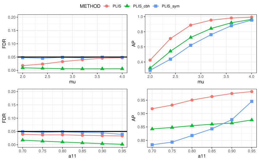
Figure 4: FDR and AP comparison for PLIS, symmetrized PLIS via contrast and PLIS without defining candidate rejection set and mirror calibration set. The null density $f_{0}$ is of $\mathcal{N}(0,1)$ and the signal’s density $f_{1}$ is of $\mathcal{N}(\mu,1)$. In the top row, we fix $a_{00}=0.9,a_{11}=0.8$ and let $\mu$ vary; $\mu=3,a_{00}=0.6$ are fixed in the second row where $a_{11}$ is changing.

In the top row, we can see that the FDR of ${\rm PLIS}_{\rm sym}$ consistently remains close to the nominal level, while ${\rm PLIS}_{\rm cbh}$ exhibits an overly conservative behavior. Our proposed method, PLIS, demonstrates conservativeness when $\mu$ is small but adaptively achieves the desired nominal FDR level as $\mu$ increases. Despite the conservativeness observed in ${\rm PLIS}_{\rm cbh}$, it outperforms ${\rm PLIS}_{\rm sym}$ in terms of average power, indicating that the rankings obtained from $s_{j}^{X}$ are superior to those derived from the contrast statistics $T_{j}=s_{j}^{Y}-s_{j}^{X}$. However, in the bottom row, as the dependence becomes stronger, the conservativeness of ${\rm PLIS}_{\rm cbh}$ becomes increasingly prominent, eventually leading to a decrease in power compared to ${\rm PLIS}_{\rm sym}$. Remarkably, our proposed method, PLIS, consistently outperforms both variations in all situations. It showcases two important advantages: first, PLIS addresses the sub-optimal ranking issue observed in ${\rm PLIS}_{\rm sym}$ by preserving the efficient ranking derived from $s_{j}^{X}$; second, PLIS alleviates the conservativeness of ${\rm PLIS}_{\rm cbh}$ by narrowing down the candidate rejection set from $\mathcal{G}$ to $\mathcal{G}^{r}$.

5 Application

In this section, we demonstrate the application of PLIS in genome-wide association studies (GWAS) for the identification of genetic variants associated with Type 1 diabetes (T1D). T1D is a common autoimmune disorder resulting from the interactions of multiple genetic and environmental risk factors. It is widely postulated that multiple genetic loci contribute to the risk of developing T1D. To systematically search for these unknown loci, a GWAS was conducted by Barrett et al. (2009), utilizing a discovery cohort consisting of 7514 cases and 9045 controls. For each single nucleotide polymorphism (SNP), the association between allele frequencies and disease status was assessed using a 1-d.f. $\chi^{2}$ test and summarized as a $p$-value. The dataset is publicly accessible at https://www.ebi.ac.uk/gwas/.

HMM-based methods have gained popularity in genomic research for modeling the complex underlying genomic structure that comprises a large number of genetic markers, such as SNPs and copy number variations (CNVs). These methods provide powerful tools for effectively identifying disease-associated markers while accounting for the dependencies between adjacent markers (Wei et al., 2009; Guan, 2014; Sesia et al., 2018; Perrot-Dockès et al., 2021). In GWAS, disease-associated SNPs tend to exhibit a higher frequency within local genomic neighborhoods than would be expected by chance, which stems from the co-inheritance of certain genetic variants along the chromosomes. By employing Model (2), particularly leveraging the capabilities of HMMs, we can capture the underlying “block” patterns between markers, thereby enabling the identification of meaningful associations that are situated in close proximity to one another.

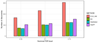
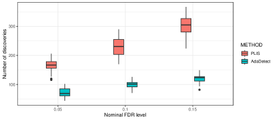
Figure 5: Number of discoveries for the T1D data. The left bar chart represents the average numbers for each method at different nominal FDR level, while the right is the boxplots for the two randomized procedures.

Our analysis focuses on the examination of the first 10,753 SNPs on Chromosome 22. The calibration data are generated independently from a $\chi^{2}(1)$ distribution, and we obtain $p$-values and $z$-values for the data by applying appropriate transformations, as outlined in Wei et al. (2009). We employ PLIS (with an HMM as the working model), BH, AdaDetect and AdaPT to identify the genetic loci associated with T1D at different FDR levels $\alpha=0.05$, $0.1$, and $0.15$. To ensure the reliability of our analysis, we apply PLIS and AdaDetect, both involve randomly generated null samples, for 100 times and report the average results. The numerical results are summarized in Figure 5. We can see that BH and AdaDetect have comparable numbers of discoveries across varying $\alpha$ levels, whereas PLIS and AdaPT exhibit improved power by leveraging the local structures within the data. Furthermore, PLIS demonstrates a marginally superior power compared to AdaPT. By effectively utilizing the inherent data structure and adopting a model-free approach, PLIS serves as a valuable tool for improving the accuracy, interpretability, and robustness of multiple testing results in genetic association studies.

Online Supplementary Material for “False Discovery Rate Control For Structured Multiple Testing: Asymmetric Rules And Conformal $Q$-values”

This supplement contains the proofs of theorems and propositions (Sections A and B), some extensions of the proposed PLIS procedure (Sections C), a comparative review of PLIS and related methods (Section D), and additional numerical results (Section E).

Appendix A A Proofs For Results in Section 2

In this section, proofs for theories in Section 2.4 and Section 2.7 are provided. And we further prove Theorem 2 for semi-supervised PLIS in Appendix C after introducing de Finetti’s Theorem (Lemma 3).

A.1 A general theory on pairwise exchangeability

To begin, we introduce some notation.

• The observed data $\mathbf{X}=(X_{j}:j\in\mathcal{G})$ and corresponding latent states $\boldsymbol{\Theta}=(\theta_{j}:j\in\mathcal{G})$ are generated from Model (2).

• Denote the null samples $\mathbf{Y}=(Y_{j}:j\in\mathcal{G})$, where $Y_{j}\overset{i.i.d.}{\sim}f_{0}$.

• Let $\mathbf{W}=(W_{j}:j\in\mathcal{G})$ be a structured data set on the same graph $\mathcal{G}$.

• We use $\mathbf{W}$ as the baseline data and construct two new data sets for every $i\in\mathcal{G}$: $\tilde{\mathbf{X}}_{i}$ and $\tilde{\mathbf{Y}}_{i}$, by substituting $X_{i}$ and $Y_{i}$ in place of $W_{i}$ in $\mathbf{W}$, respectively.

• Denote $s_{i}^{X}$($s_{i}^{Y}$) the scores computed based on $\tilde{\mathbf{X}}_{i}$ and $\tilde{\mathbf{Y}}_{i}$: $s_{i}^{X}=g_{i}(\tilde{\mathbf{X}}_{i})$ and $s_{i}^{Y}=g_{i}(\tilde{\mathbf{Y}}_{i})$ for $i\in\mathcal{G}$, where $\{g_{i}(\cdot):i\in\mathcal{G}\}$ are a class of functions that are $\mathbf{W}$-measurable (including non-random functions).

• Let $\mathbf{S}_{-i}=\{s_{j}^{X},s_{j}^{Y}:j\neq i,j\in\mathcal{G}\}$.

• Let $Z_{i}=\{X_{i},Y_{i}\}$ denote a set with two elements and $Z_{i}^{\prime}=(X_{i},Y_{i})$ denote a 2-dimensional vector.

• Denote $T_{i}=\{X_{i},Y_{i},W_{i}\}$ a set of variables with three elements and $T_{i}^{\prime}=(X_{i},Y_{i},W_{i})$ a 3-dimensional vector.

The following lemma provides a useful result on pairwise exchangeability.

Lemma 1.

Suppose the following two conditions hold: (i) $\{T_{j}:j\in\mathcal{G}\}$ are mutually independent conditional on $\boldsymbol{\Theta}$, and (ii) for $i\in\mathcal{H}_{0}$, $(X_{i},Y_{i},W_{i})\overset{d}{=}(Y_{i},X_{i},W_{i})$. Then

1. $\{Z_{j}=\{X_{j},Y_{j}\}:j\in\mathcal{G}\}$ are conditionally independent given $\mathbf{W}$ and $\boldsymbol{\Theta}$, and for $i\in\mathcal{H}_{0}$, $(X_{i},Y_{i}|\mathbf{W},\boldsymbol{\Theta})\overset{d}{=}(Y_{i},X_{i}|\mathbf{W},\boldsymbol{\Theta})$.

2. $\{\mathcal{D}_{j}=\{\tilde{\mathbf{X}}_{j},\tilde{\mathbf{Y}}_{j}\}:j\in\mathcal{G}\}$ are conditionally independent given $\mathbf{W}$ and $\boldsymbol{\Theta}$, and for $i\in\mathcal{H}_{0}$, $(\tilde{\mathbf{X}}_{i},\tilde{\mathbf{Y}}_{i}|\mathbf{W},\boldsymbol{\Theta})\overset{d}{=}(\tilde{\mathbf{Y}}_{i},\tilde{\mathbf{X}}_{i}|\mathbf{W},\boldsymbol{\Theta})$.

3. Denote $\mathbf{s}_{j}=\{s_{j}^{X},s_{j}^{Y}\}$ for $j\in\mathcal{G}$. Then $\{\mathbf{s}_{j}:j\in\mathcal{G}\}$ are conditionally independent given $\mathbf{W}$ and $\boldsymbol{\Theta}$, and for $i\in\mathcal{H}_{0}$, $s_{i}^{X}$ and $s_{i}^{Y}$ are exchangeable conditional on other scores, i.e., $(s_{i}^{X},s_{i}^{Y}|\mathbf{S}_{-i})\overset{d}{=}(s_{i}^{Y},s_{i}^{X}|\mathbf{S}_{-i})$, or equivalently $(s_{i}^{X},s_{i}^{Y},\mathbf{S}_{-i})\overset{d}{=}(s_{i}^{Y},s_{i}^{X},\mathbf{S}_{-i})$.

A.2 Proof of Lemma 1

Proof of Lemma 1.

Note that $T_{i}^{\prime}=(Z_{i}^{\prime},W_{i})$. Given Condition (i), we can conclude that $\{T_{j}^{\prime}:j\in\mathcal{G}\}$ are mutually independent conditional on $\boldsymbol{\Theta}$. For $j\in\mathcal{G}$, let $A_{j}$ denote a Borel set on $\mathbb{R}^{2}$, and let $B_{j}$ denote a Borel set on $\mathbb{R}$. Additionally, let $B^{(m)}$ denote the Cartesian product of $\{B_{j},j\in\mathcal{G}\}$. Then we have

$$\begin{split}&\mathbb{P}(Z_{i}^{\prime}\in A_{i},i\in\mathcal{G}|\mathbf{W}\in B^{(m)},\boldsymbol{\Theta})\\ =&\frac{1}{\mathbb{P}(\mathbf{W}\in B^{(m)}|\boldsymbol{\Theta})}\mathbb{P}(Z_{i}^{\prime}\in A_{i},i\in\mathcal{G},\mathbf{W}\in B^{(m)}|\boldsymbol{\Theta})\\ =&\frac{1}{\mathbb{P}(\mathbf{W}\in B^{(m)}|\boldsymbol{\Theta})}\mathbb{P}(T_{i}^{\prime}\in A_{i}\times B_{i},i\in\mathcal{G}|\boldsymbol{\Theta})\\ =&\frac{1}{\mathbb{P}(\mathbf{W}\in B^{(m)}|\boldsymbol{\Theta})}\prod_{i\in\mathcal{G}}\mathbb{P}(T_{i}^{\prime}\in A_{i}\times B_{i}|\boldsymbol{\Theta})\\ =&\frac{1}{\mathbb{P}(\mathbf{W}\in B^{(m)}|\boldsymbol{\Theta})}\prod_{i\in\mathcal{G}}\left[\mathbb{P}(Z_{i}^{\prime}\in A_{i}|W_{i}\in B_{i},\boldsymbol{\Theta})\mathbb{P}(W_{i}\in B_{i}|\boldsymbol{\Theta})\right]\\ =&\frac{1}{\mathbb{P}(\mathbf{W}\in B^{(m)}|\boldsymbol{\Theta})}\left(\prod_{i\in\mathcal{G}}\mathbb{P}(W_{i}\in B_{i}|\boldsymbol{\Theta})\right)\left(\prod_{i\in\mathcal{G}}\mathbb{P}(Z_{i}^{\prime}\in A_{i}|\mathbf{W}\in B^{(m)},\boldsymbol{\Theta})\right)\\ =&\prod_{i\in\mathcal{G}}\mathbb{P}(Z_{i}^{\prime}\in A_{i}|\mathbf{W}\in B^{(m)},\boldsymbol{\Theta}).\end{split}$$

Note that the preceding calculations apply to any Borel sets $A_{j}$ and $B_{j}$, which implies that $\{Z_{i}^{\prime}:i\in\mathcal{G}\}$ are conditionally independent given $\mathbf{W}$ and $\boldsymbol{\Theta}$. This result leads to the conclusion that $\{Z_{i}:i\in\mathcal{G}\}$ are conditionally independent given $\mathbf{W}$ and $\boldsymbol{\Theta}$.

For $i\in\mathcal{H}_{0}$, since $(X_{i},Y_{i},W_{i})\overset{d}{=}(Y_{i},X_{i},W_{i})$, we have

$$(X_{i},Y_{i}|\mathbf{W},\boldsymbol{\Theta})\overset{d}{=}(X_{i},Y_{i}|W_{i},\boldsymbol{\Theta})\overset{d}{=}(Y_{i},X_{i}|W_{i},\boldsymbol{\Theta})\overset{d}{=}(Y_{i},X_{i}|\mathbf{W},\boldsymbol{\Theta}),$$

where the first and last steps follow from Condition (i).

Let $\mathcal{D}_{i}=\{\tilde{\mathbf{X}}_{i},\tilde{\mathbf{Y}}_{i}\}$, $\mathcal{D}=\{\mathcal{D}_{i}:i\in\mathcal{G}\}$, and $\mathcal{D}_{-i}=\mathcal{D}\backslash\mathcal{D}_{i}$. We assert that $\mathcal{D}_{i}$ is conditionally independent of $\mathcal{D}_{-i}$ given $\mathbf{W}$ and $\boldsymbol{\Theta}$. This is due to the fact that, given $\mathbf{W}$ and $\boldsymbol{\Theta}$, the randomness of the components in $\mathcal{D}$ solely arises from $\{Z_{i}:i\in\mathcal{G}\}$. Moreover, the elements $Z_{i}$ are conditionally independent, thereby establishing the conditional independence between $\mathcal{D}_{i}$ and $\mathcal{D}_{-i}$.

Now, let us examine the scores $s_{i}^{X}\equiv g_{i}(\tilde{\mathbf{X}}_{i})$ and $s_{i}^{Y}\equiv g_{i}(\tilde{\mathbf{Y}}_{i})$, $i\in\mathcal{G}$. Let $\mathbf{s}_{i}=\{s_{i}^{X},s_{i}^{Y}\}$. Based on the conditional independence between $\mathcal{D}_{i}$ and $\mathcal{D}_{-i}$ given $\mathbf{W}$ and $\boldsymbol{\Theta}$, we infer that

$$m \{\mathbf{s}_{i}:i\in\mathcal{G}\} \mathbf{W} \boldsymbol{\Theta}$$ components of are mutually independent conditional on and . (A.1)

This result is due to the fact that $\mathbf{s}_{i}$ is a function of $\mathcal{D}_{i}$, and $g_{i}(\cdot)$ is $\mathbf{W}$-measurable.

For $i\in\mathcal{H}_{0}$, it holds that $(X_{i},Y_{i}|\mathbf{W},\boldsymbol{\Theta})\overset{d}{=}(Y_{i},X_{i}|\mathbf{W},\boldsymbol{\Theta})$. Consequently, we can deduce that $(\tilde{\mathbf{X}}_{i},\tilde{\mathbf{Y}}_{i}|\mathbf{W},\boldsymbol{\Theta})\overset{d}{=}(\tilde{\mathbf{Y}}_{i},\tilde{\mathbf{X}}_{i}|\mathbf{W},\boldsymbol{\Theta})$. As a result, the scores $s_{i}^{X}$ and $s_{i}^{Y}$ must satisfy

$$(s_{i}^{X}|\mathbf{W},\boldsymbol{\Theta})\overset{d}{=}(s_{i}^{Y}|\mathbf{W},\boldsymbol{\Theta}).$$ (A.2)

Let $\mathbf{S}_{-i}=\{\mathbf{s}_{j}:j\in\mathcal{G},j\neq i\}$. It can be shown that

$$(s_{i}^{X},s_{i}^{Y}|\mathbf{S}_{-i},\mathbf{W},\boldsymbol{\Theta})\overset{d}{=}(s_{i}^{X},s_{i}^{Y}|\mathbf{W},\boldsymbol{\Theta})\overset{d}{=}(s_{i}^{Y},s_{i}^{X}|\mathbf{W},\boldsymbol{\Theta})\overset{d}{=}(s_{i}^{Y},s_{i}^{X}|\mathbf{S}_{-i},\mathbf{W},\boldsymbol{\Theta}),$$

where the first and last steps follow from (A.1), and the second step follows from (A.2).

After integrating out $(\mathbf{W},\boldsymbol{\Theta})$, we can obtain $(s_{i}^{X},s_{i}^{Y}|\mathbf{S}_{-i})\overset{d}{=}(s_{i}^{Y},s_{i}^{X}|\mathbf{S}_{-i})$, which establishes the desired result on pairwise exchangeability:

$$(s_{i}^{X},s_{i}^{Y},\mathbf{S}_{-i})\overset{d}{=}(s_{i}^{Y},s_{i}^{X},\mathbf{S}_{-i}) i\in\mathcal{H}_{0}$$ for .

∎

A.3 Justifications of Properties 1-3

Properties 1-3 are intermediate conclusions through the proof of Lemma 1. Note that the scores $s_{i}^{X}$ and $s_{i}^{Y}$ defined in Algorithm 1 are specific examples of the scores defined in Lemma 1. Specifically, Algorithm 1 takes $g_{i}(\cdot)=\mathbb{P}_{\mathcal{M,A}}(\theta_{i}=0|\cdot)$ for $i\in\mathcal{G}$. Hence the properties can be established by verifying the two conditions of Lemma 1, for $W_{i}$ constructed based on a symmetric function $h(x,y)=h(y,x)$ in Algorithm 1.

To establish Condition (i), we consider any bivariate function $h$ and assume that $W_{i}=h(X_{i},Y_{i})$ for $i\in\mathcal{G}$. In this case, the conditional independence assumption of $\{T_{i}=\{X_{i},Y_{i},W_{i}\}:i\in\mathcal{G}\}$ holds trivially. This is due to the fact that $\{Z_{i}=\{X_{i},Y_{i}\}:i\in\mathcal{G}\}$ are mutually independent given $\boldsymbol{\Theta}$, and $W_{i}$ is a function of $Z_{i}$.

To establish Condition (ii), it should be noted that the function $h(x,y)$ defined by (5) is used to construct $\mathbf{W}$ in the PLIS procedure (Algorithm 1). As $h(x,y)$ is a symmetric function and $X_{i}$ and $Y_{i}$ are i.i.d. for any $i\in\mathcal{H}_{0}$, it follows that

$$(X_{i},Y_{i},W_{i})=(X_{i},Y_{i},h(X_{i},Y_{i}))\overset{d}{=}(Y_{i},X_{i},h(Y_{i},X_{i}))=(Y_{i},X_{i},h(X_{i},Y_{i}))=(Y_{i},X_{i},W_{i}),$$

establishing Condition (ii).

Finally, Properties 1-3 on exchangeability can be justified by following the arguments in the proof of Lemma 1.

A.4 Proof of Theorem 1

Proof.

Note that PLIS searches for a threshold utilizing

$$\tau=\sup\{t\in\mathbf{S}_{X}\cup\mathbf{S}_{Y}:Q(t)\leq\alpha\},$$

which guarantees that $Q(\tau)\leq\alpha$ holds true at all times. Moreover, we have

$$\begin{split}\mathrm{FDP}(\tau)&=\frac{\sum_{j\in\mathcal{G}^{r}\cap\mathcal{H}_{0}}\mathbb{I}\{s_{j}^{X}\leq\tau\}}{(\sum_{j\in\mathcal{G}^{r}}\mathbb{I}\{s_{j}^{X}\leq\tau\})\vee 1}\\ &=Q(\tau)\frac{1+\sum_{j\in\mathcal{G}^{c}\cap\mathcal{H}_{0}}\mathbb{I}\{s_{j}^{Y}\leq\tau\}}{1+\sum_{j\in\mathcal{G}^{c}}\mathbb{I}\{s_{j}^{Y}\leq\tau\}}\frac{\sum_{j\in\mathcal{G}^{r}\cap\mathcal{H}_{0}}\mathbb{I}\{s_{j}^{X}\leq\tau\}}{1+\sum_{j\in\mathcal{G}^{c}\cap\mathcal{H}_{0}}\mathbb{I}\{s_{j}^{Y}\leq\tau\}}\\ &\leq\alpha\cdot 1\cdot\frac{\sum_{j\in\mathcal{G}^{r}\cap\mathcal{H}_{0}}\mathbb{I}\{s_{j}^{X}\leq\tau\}}{1+\sum_{j\in\mathcal{G}^{c}\cap\mathcal{H}_{0}}\mathbb{I}\{s_{j}^{Y}\leq\tau\}}.\end{split}$$

To show $\mathrm{FDR}=\mathbb{E}[\mathrm{FDP}(\tau)]\leq\alpha$, consider the following quantity

$$M(t)=\frac{\sum_{j\in\mathcal{G}^{r}\cap\mathcal{H}_{0}}\mathbb{I}\{s_{j}^{X}\leq t\}}{1+\sum_{j\in\mathcal{G}^{c}\cap\mathcal{H}_{0}}\mathbb{I}\{s_{j}^{Y}\leq t\}}.$$

It follows that we only need to prove that

$$\mathbb{E}M(\tau)=\mathbb{E}\left[\frac{\sum_{j\in\mathcal{G}^{r}\cap\mathcal{H}_{0}}\mathbb{I}\{s_{j}^{X}\leq\tau\}}{1+\sum_{j\in\mathcal{G}^{c}\cap\mathcal{H}_{0}}\mathbb{I}\{s_{j}^{Y}\leq\tau\}}\right]\leq 1.$$ (A.3)

The inequality presented in (A.3) will be established by leveraging well-established martingale theories. To start with, we present and prove three claims in turn, all of which are instrumental in the development of our theory.

A.4.1 Statement and Proof of Claim 1

Claim 1. Consider the scores $\{s_{j}^{X},s_{j}^{Y}:j\in\mathcal{G}\}$ generated by Algorithm 1. Define

$$S_{j}=S(s_{j}^{X},s_{j}^{Y})=\mathrm{sign}(s_{j}^{Y}-s_{j}^{X})\cdot[g(s_{j}^{X})\vee g(s_{j}^{Y})],\quad\forall j\in\mathcal{G},$$ (A.4)

where $g(\cdot):\mathbb{R}_{\geq 0}\to\mathbb{R}_{\geq 0}$ is a non-random strictly decreasing function. Consider the following mirror process

$$Q^{S}(t)=\frac{1+\sum_{j\in\mathcal{G}}\mathbb{I}\{S_{j}\leq-t\}}{(\sum_{j\in\mathcal{G}}\mathbb{I}\{S_{j}\geq t\})\vee 1},\quad t>0.$$ (A.5)

Define $\tau^{\prime}=\inf\{t\in\mathcal{S}:Q^{S}(t)\leq\alpha\}$, where $\mathcal{S}=\{|S_{j}|:j\in\mathcal{G}\}$. Consider a decision rule ${\boldsymbol{\delta}}^{\prime}=\{\delta_{j}^{\prime}:j\in\mathcal{G}\}$, where $\delta_{j}^{\prime}=\mathbb{I}\{S_{i}\geq\tau^{\prime}\}$. Then ${\boldsymbol{\delta}}^{\prime}$ is equivalent to the decision rule $\boldsymbol{\delta}=\{\delta_{j}:j\in\mathcal{G}\}$ output by Algorithm 1.

Proof of Claim 1.

For a non-random strictly decreasing function $g(\cdot)$ defined on $\mathbb{R}_{\geq 0}\to\mathbb{R}_{\geq 0}$, the value $g(s_{i}^{X})$ can be interpreted as a non-conformity score, with a higher value indicating stronger evidence against $H_{0,i}$. As such $g(\cdot)$ is bijective, we have

$$\mathcal{G}^{r} = \{i\in\mathcal{G}:s_{i}^{X}<s_{i}^{Y}\}=\{i\in\mathcal{G}:g(s_{i}^{X})>g(s_{i}^{Y})\},\mbox{ and}$$

$$\mathcal{G}^{c} = \{i\in\mathcal{G}:s_{i}^{Y}<s_{i}^{X}\}=\{i\in\mathcal{G}:g(s_{i}^{Y})>g(s_{i}^{X})\}.$$

Recall the mirror process $Q(t)$ defined in (6) and the decision $\delta_{i}$ output by Algorithm 1, we have $\delta_{i}=\mathbb{I}\{s_{i}^{X}\leq\tau\}\mathbb{I}\{s_{i}^{X}<s_{i}^{Y}\}=\mathbb{I}\{g(s_{i}^{X})\geq\tau^{\prime}\}\mathbb{I}\{g(s_{i}^{X})>g(s_{i}^{Y})\}$, where

$$\tau^{\prime}=\inf\left\{t\in\{g(s_{i}^{X})\}_{i\in\mathcal{G}^{r}}\cup\{g(s_{i}^{Y})\}_{i\in\mathcal{G}^{c}}:\frac{1+\sum_{j\in\mathcal{G}}\mathbb{I}\{g(s_{j}^{Y})\geq t\}\mathbb{I}\{s_{j}^{Y}<s_{j}^{X}\}}{(\sum_{j\in\mathcal{G}}\mathbb{I}\{g(s_{j}^{X})\geq t\}\mathbb{I}\{s_{j}^{X}<s_{j}^{Y}\})\vee 1}\leq\alpha\right\}.$$

This holds because $g(\cdot)$ is strictly decreasing, and that the function

$$\frac{1+\sum_{j\in\mathcal{G}}\mathbb{I}\{g(s_{j}^{Y})\geq t\}\mathbb{I}\{s_{j}^{Y}<s_{j}^{X}\}}{(\sum_{j\in\mathcal{G}}\mathbb{I}\{g(s_{j}^{X})\geq t\}\mathbb{I}\{s_{j}^{X}<s_{j}^{Y}\})\vee 1}$$

only jumps at points within the set $\{g(s_{i}^{X})\}_{i\in\mathcal{G}^{r}}\cup\{g(s_{i}^{Y})\}_{i\in\mathcal{G}^{c}}$. By the definition of $S_{j}$ in (A.4), we have that, for any $t>0$:

$$S_{j}\geq t \Longleftrightarrow s_{j}^{X}<s_{j}^{Y}\mbox{ and }g(s_{j}^{X})\geq t,$$

$$S_{j}\leq-t \Longleftrightarrow s_{j}^{Y}<s_{j}^{X}\mbox{ and }g(s_{j}^{Y})\geq t.$$

It follows that

$$\frac{1+\sum_{j\in\mathcal{G}}\mathbb{I}\{g(s_{j}^{Y})\geq t\}\mathbb{I}\{s_{j}^{Y}<s_{j}^{X}\}}{(\sum_{j\in\mathcal{G}}\mathbb{I}\{g(s_{j}^{X})\geq t\}\mathbb{I}\{s_{j}^{X}<s_{j}^{Y}\})\vee 1}=\frac{1+\sum_{j\in\mathcal{G}}\mathbb{I}\{S_{j}\leq-t\}}{(\sum_{j\in\mathcal{G}}\mathbb{I}\{S_{j}\geq t\})\vee 1}=Q^{S}(t),\quad t>0.$$

It is easy to see that $\mathcal{S}=\{g(s_{i}^{X})\}_{i\in\mathcal{G}^{r}}\cup\{g(s_{i}^{Y})\}_{i\in\mathcal{G}^{c}}$. Therefore we have $\tau^{\prime}=\inf\{t\in\mathcal{S}:Q^{S}(t)\leq\alpha\}$ and

$$\delta_{i}=\mathbb{I}\{s_{i}^{X}\leq\tau\}\mathbb{I}\{s_{i}^{X}<s_{i}^{Y}\}=\mathbb{I}\{S_{i}\geq\tau^{\prime}\}=\delta_{i}^{\prime},$$

completing the proof. ∎

A.4.2 An equivalent formulation

Let $|S_{(1)}|\leq|S_{(2)}|\leq\cdots\leq|S_{(m)}|$ denote the order statistics of $\{|S_{j}|:j\in\mathcal{G}\}$. Define

$$\hat{k}=\min\{i\in[m]:Q^{S}(|S_{(i)}|)\leq\alpha\},$$ (A.6)

where $m=|\mathcal{G}|$ denotes the total number of hypotheses. Since $Q^{S}(t)$ jumps at points only within the set $\mathcal{S}=\{|S_{j}|:j\in\mathcal{G}\}$, the decision rule output by Algorithm 1 is equivalent to a decision rule that rejects $H_{0,i}$ if $S_{j}\geq|S_{(\hat{k})}|$. Furthermore, we introduce the mapping $\rho:[m]\to\mathcal{G}$ as follows: for each $k\in[m]$, $\rho(k)=l\in\mathcal{G}$ whenever $|S_{(k)}|=|S_{l}|$. We claim that $|S_{(i)}|$ is null if $\rho(i)\in\mathcal{H}_{0}$, and non-null if $\rho(i)\notin\mathcal{H}_{0}$. By convention, we set the initial value as $|S_{(0)}|=0$.

In Claim 1, we have established that

$$\mathbb{E}M(\tau)=\mathbb{E}\left[\frac{\sum_{j\in\mathcal{G}^{r}\cap\mathcal{H}_{0}}\mathbb{I}\{s_{j}^{X}\leq\tau\}}{1+\sum_{j\in\mathcal{G}^{c}\cap\mathcal{H}_{0}}\mathbb{I}\{s_{j}^{Y}\leq\tau\}}\right]=\mathbb{E}\left[\frac{\sum_{j\in\mathcal{H}_{0}}\mathbb{I}\{S_{j}\geq\tau^{\prime}\}}{1+\sum_{j\in\mathcal{H}_{0}}\mathbb{I}\{S_{j}\leq-\tau^{\prime}\}}\right].$$

Denote $V^{X}(t)=\sum_{j\in\mathcal{H}_{0}}\mathbb{I}\{S_{j}\geq t\}$ and $V^{Y}(t)=\sum_{j\in\mathcal{H}_{0}}\mathbb{I}\{S_{j}\leq-t\}$. By (A.6), the inequality (A.3) would be established if the following holds:

$$\mathbb{E}\left[\frac{V^{X}(\tau^{\prime})}{1+V^{Y}(\tau^{\prime})}\right]=\mathbb{E}\left[\frac{V^{X}(|S_{(\hat{k})}|)}{1+V^{Y}(|S_{(\hat{k})}|)}\right]\leq 1.$$

A.4.3 Statement and proof of Claim 2

Claim 2. Denote $\mathcal{F}_{0}=\sigma\left(\{S_{j}:j\notin\mathcal{H}_{0}\},\{|S_{j}|:j\in\mathcal{G}\}\right)$. Consider the filtration $\mathcal{F}=(\mathcal{F}_{k})_{k=0,1,\cdots,m}$, where $\mathcal{F}_{k}$ is generated by

$$\mathcal{F}_{k}=\sigma\Big{(}\mathcal{F}_{0}\cup\sigma\left(V^{X}(|S_{({i})}|),V^{Y}(|S_{({i})}|):1\leq i\leq k\right)\Big{)},\quad k\geq 1.$$

Then the discrete-time random process $(M^{S}_{k})_{k=0,1,\cdots,m}$ defined by

$$M^{S}_{k}=\frac{V^{X}(|S_{({k})}|)}{1+V^{Y}(|S_{({k})}|)},$$

is a super-martingale with respect to the filtration $\mathcal{F}$.

The proof of Claim 2 relies on a useful lemma established by Barber and Candès (2015). The proof of the lemma is omitted.

Lemma 2.

For any anti-symmetric function $f(x,y)$ satisfying $f(x,y)=-f(y,x)$, if the scores $(s_{i}^{X}:i\in\mathcal{G})$ and $(s_{i}^{Y}:i\in\mathcal{G})$ are pairwise exchangeable under the null, i.e., (7) holds, then $(\mathrm{sign}(f(s_{i}^{X},s_{i}^{Y})):i\in\mathcal{H}_{0})$ are i.i.d. coin flips conditional on $(|f(s_{i}^{X},s_{i}^{Y})|:i\in\mathcal{G})$.

Proof of Claim 2.

By the definition of $V^{X}(|S_{(k)}|)$ and $V^{Y}(|S_{(k)}|)$, we have

$$0\leq V^{X}(|S_{(i+1)}|)\leq V^{X}(|S_{(i)}|),\quad 0\leq V^{Y}(|S_{(i+1)}|)\leq V^{Y}(|S_{(i)}|),\quad\forall i=1,\cdots,m-1.$$

To evaluate $\mathbb{E}[M_{k+1}^{S}|\mathcal{F}_{k}]$, we consider two situations.

Situation 1: $V^{Y}(|S_{(k)}|)=0$. In this case, we have $M_{k}^{S}=V^{X}(|S_{(k)}|)$. It follows that

$$M_{k+1}^{S}=\frac{V^{X}(|S_{(k+1)}|)}{1+V^{Y}(|S_{(k+1)}|)}=V^{X}(|S_{(k+1)}|)\leq V^{X}(|S_{(k)}|)=M_{k}^{S}$$

almost surely. Therefore we must have

$$\mathbb{E}[M_{k+1}^{S}|\mathcal{F}_{k}]\leq\mathbb{E}[M_{k}^{S}|\mathcal{F}_{k}]=M_{k}^{S}.$$

Situation 2: $V^{Y}(|S_{(k)}|)\neq 0$. In this case, we first check the definition of $S_{j}=S(s_{j}^{X},s_{j}^{Y})$ in (A.4), where the bivariate function $S(x,y)=\mathrm{sign}(y-x)\cdot[g(x)\vee g(y)]$ is anti-symmetric, i.e., $S(x,y)=-S(y,x)$. By Lemma 2, we have that $(\mathrm{sign}(S_{j}):j\in\mathcal{H}_{0})$ are i.i.d. coin flips conditional on $(|S_{j}|:j\in\mathcal{G})$, and therefore exchangeable. If $|S_{(k)}|$ corresponds to a non-null score, i.e., $\rho(k)\notin\mathcal{H}_{0}$, then $V^{X}(|S_{(k+1)}|)=V^{X}(|S_{(k)}|)$ and $V^{Y}(|S_{(k+1)}|)=V^{Y}(|S_{(k)}|)$, so $M_{k+1}^{S}=M_{k}^{S}$ almost surely. On the other hand, if $|S_{(k)}|$ corresponds to a null score, i.e., $\rho(k)\in\mathcal{H}_{0}$, then according to the exchangeability between $(\mathrm{sign}(S_{j}):j\in\mathcal{H}_{0})$, we have

$$\mathbb{P}\Big{(}V^{X}(|S_{(k+1)}|) = V^{X}(|S_{(k)}|)-1,V^{Y}(|S_{(k+1)}|)=V^{Y}(|S_{(k)}|)\Big{|}\mathcal{F}_{k}\Big{)}=\frac{V^{X}(|S_{(k)}|)}{V^{X}(|S_{(k)}|)+V^{Y}(|S_{(k)}|)},$$

$$\mathbb{P}\Big{(}V^{X}(|S_{(k+1)}|) = V^{X}(|S_{(k)}|),V^{Y}(|S_{(k+1)}|)=V^{Y}(|S_{(k)}|)-1\Big{|}\mathcal{F}_{k}\Big{)}=\frac{V^{Y}(|S_{(k)}|)}{V^{X}(|S_{(k)}|)+V^{Y}(|S_{(k)}|)}.$$

It follows that the conditional expectation can be calculated as

$$\mathbb{E}[M_{k+1}^{S}|\mathcal{F}_{k}]$$

$$= \frac{V^{X}(|S_{(k)}|-1}{1+V^{Y}(|S_{(k)}|)}\cdot\frac{V^{X}(|S_{(k)}|)}{V^{X}(|S_{(k)}|)+V^{Y}(|S_{(k)}|)}+\frac{V^{X}(|S_{(k)}|}{1+V^{Y}(|S_{(k)}|)-1}\cdot\frac{V^{Y}(|S_{(k)}|)}{V^{X}(|S_{(k)}|)+V^{Y}(|S_{(k)}|)}$$

$$= \frac{V^{X}(|S_{(k)}|)}{V^{X}(|S_{(k)}|)+V^{Y}(|S_{(k)}|)}\left[1+\frac{V^{X}(|S_{(k)}|-1}{1+V^{Y}(|S_{(k)}|)}\right]$$

$$= \frac{V^{X}(|S_{(k)}|)}{1+V^{Y}(|S_{(k)}|)}=M_{k}^{S}.$$

In all situations, we have $\mathbb{E}[M_{k+1}^{S}|\mathcal{F}_{k}]\leq M_{k}^{S},$ which establishes that the random process $(M^{S}_{k})_{k=0,1,\cdots,m}$ is a super-martingale. ∎

A.4.4 Statement and Proof of Claim 3

Claim 3. $\mathbb{E}[M_{\hat{k}}^{S}]\leq 1$.

Proof of Claim 3.

Recall that $\hat{k}=\min\{i\in[m]:Q^{S}(|S_{(i)}|)\leq\alpha\}$, where $Q^{S}(t)$ is defined in equation (A.5). It is easy to see that $\hat{k}$ is an $\mathcal{F}$-stopping time, as knowing $\{S_{j}:j\notin\mathcal{H}_{0}\}$, $\{|S_{j}|:j\in\mathcal{G}\}$ and $\{V^{X}(|S_{(i)}|),V^{Y}(|S_{(i)}|):i\leq K\}$ is sufficient to determine whether the event $\{\hat{k}=K\}$ occurs.

By Lemma 2, $\left\{\mathrm{sign}(S_{j}):j\in\mathcal{H}_{0}\right\}$ are exchangeable coin flips, indicating that $|\mathcal{G}^{r}\cap\mathcal{H}_{0}|=\sum_{j\in\mathcal{H}_{0}}\mathbb{I}\{\mathrm{sign}(S_{j})=+1\}\sim B(|\mathcal{H}_{0}|,1/2)$ given $\mathcal{F}_{0}=\sigma\left(\{S_{j}:j\notin\mathcal{H}_{0}\},\{|S_{j}|:j\in\mathcal{G}\}\right)$. Consider a binomial variable $B\sim B(n,1/2)$, then we have

$$\begin{split}\mathbb{E}\Big{[}\frac{B}{1+n-B}\Big{]}&=\sum_{j=1}^{n}\mathbb{P}(B=i)\frac{j}{1+n-j}\\ &=\Big{(}\frac{1}{2}\Big{)}^{n}\sum_{j=1}^{n}\frac{n!}{(n-j)!j!}\frac{j}{1+n-j}\\ &=\Big{(}\frac{1}{2}\Big{)}^{n}\sum_{j=1}^{n}\frac{n!}{(n+1-j)!(j-1)!}\\ &=\sum_{j=1}^{n}\mathbb{P}(B=i-1)\\ &=1-\Big{(}\frac{1}{2}\Big{)}^{n}\leq 1.\end{split}$$

Finally, since $(M^{S}_{k})_{k=0,1,\cdots,m}$ is an $\mathcal{F}$-super-martingale, we can invoke Doob’s optional stopping time theorem to establish that

$$\mathbb{E}\left(M_{\hat{k}}^{S}\right)\leq\mathbb{E}\{\mathbb{E}[M_{0}^{S}|\mathcal{F}_{0}]\}=\mathbb{E}\Big{\{}\mathbb{E}\Big{[}\frac{|\mathcal{G}^{r}\cap\mathcal{H}_{0}|}{1+|\mathcal{H}_{0}|-|\mathcal{G}^{r}\cap\mathcal{H}_{0}|}\Big{|}\mathcal{F}_{0}\Big{]}\Big{\}}\leq 1,$$

completing the proof. ∎

A.4.5 Proof of Theorem 1

Combining Claims 1-3, we have the following in order:

$$\begin{split}\mathbb{E}M(\tau)&=\mathbb{E}\left[\frac{\sum_{j\in\mathcal{G}^{r}\cap\mathcal{H}_{0}}\mathbb{I}\{s_{j}^{X}\leq\tau\}}{1+\sum_{j\in\mathcal{G}^{c}\cap\mathcal{H}_{0}}\mathbb{I}\{s_{j}^{Y}\leq\tau\}}\right]=\mathbb{E}\left[\frac{\sum_{j\in\mathcal{H}_{0}}\mathbb{I}\{S_{j}\geq\tau^{\prime}\}}{1+\sum_{j\in\mathcal{H}_{0}}\mathbb{I}\{S_{j}\leq-\tau^{\prime}\}}\right]\\ &=\mathbb{E}\left[\frac{V^{X}(|S_{(\hat{k})}|)}{1+V^{Y}(|S_{(\hat{k})}|)}\right]=\mathbb{E}\left(M_{\hat{k}}^{S}\right)\leq 1,\end{split}$$

establishing the desired result in (A.3), and the proof of the theorem is complete. ∎

A.5 Proof of Proposition 1

Proof of Proposition 1.

First, for each $\delta_{i}$, if $\delta_{i}=\mathbb{I}\{s_{i}^{X}\leq\tau\}\mathbb{I}\{s_{i}^{X}<s_{i}^{Y}\}=1$, we must have $i\in\mathcal{G}^{r}$. By the definition of $\tau$, we have that

$$q_{i}=\min_{t\in\mathbf{S}_{X}\cup\mathbf{S}_{Y},t\geq s_{i}^{X}}Q(t)\leq Q(\tau)\leq\alpha.$$

It follows that $\mathbb{I}\{q_{i}\leq\alpha\}=1$.

Next, if $\mathbb{I}\{q_{i}\leq\alpha\}=1$, then we have that $i\in\mathcal{G}^{r}=\{i\in\mathcal{G}:s_{i}^{X}<s_{i}^{Y}\}$, and $\min_{t\geq s_{i}^{X}}Q(t)\leq\alpha$. Since $Q(t)$ may only jump at anywhere in a subset of $\mathbf{S}_{X}\cup\mathbf{S}_{Y}$, it follows that

$$\tau=\sup\{t\in\mathbf{S}_{X}\cup\mathbf{S}_{Y}:Q(t)\leq\alpha\}\geq s_{i}^{X},$$

implying that $\mathbb{I}\{s_{i}^{X}\leq\tau\}\mathbb{I}\{s_{i}^{X}<s_{i}^{Y}\}=1$.

Combining the two arguments above, we conclude that $\delta_{i}=\mathbb{I}\{s_{i}^{X}\leq\tau\}\mathbb{I}\{s_{i}^{X}<s_{i}^{Y}\}=\mathbb{I}\{q_{i}\leq\alpha\}$ for $i\in\mathcal{G}$, establishing the equivalence of the two algorithms. ∎

Appendix B B Proofs For Results in Section 3

B.1 Proof of Theorem 3

Proof of Theorem 3.

To prove Theorem 3, we only need to show that $\mathbb{E}\big{[}\sum_{j\in\mathcal{H}_{0}}e_{j}\big{]}\leq m$. Following the steps outlined in the proof of Theorem 1, we have

$$\mathbb{E}\big{[}\sum_{j\in\mathcal{H}_{0}}e_{j}\big{]}=m\mathbb{E}\left[\sum_{j\in\mathcal{H}_{0}}\frac{\mathbb{I}\{s_{j}^{X}\leq\tau\}\mathbb{I}\{j\in\mathcal{G}^{r}\}}{1+\sum_{j\in\mathcal{G}^{c}}\mathbb{I}\{s_{j}^{Y}\leq\tau\}}\right]\leq m\mathbb{E}\left[\frac{\sum_{j\in\mathcal{G}^{r}\cap\mathcal{H}_{0}}\mathbb{I}\{s_{j}^{X}\leq\tau\}}{1+\sum_{j\in\mathcal{G}^{c}\cap\mathcal{H}_{0}}\mathbb{I}\{s_{j}^{Y}\leq\tau\}}\right]\leq m,$$

completing the proof. ∎

B.2 Proof of Proposition 2

Proof of Proposition 2.

Let $R=|\mathcal{R}|$. By the definition of $\tau$, we have

$$\frac{1+\sum_{j\in\mathcal{G}^{c}}\mathbb{I}\{s_{j}^{Y}\leq\tau\}}{R}\leq\alpha.$$

It follows that for $j\in\mathcal{R}\subset\mathcal{G}^{r}$,

$$e_{j}=\frac{m\mathbb{I}\{s_{j}^{X}\leq\tau\}}{1+\sum_{j\in\mathcal{G}^{c}}\mathbb{I}\{s_{j}^{Y}\leq\tau\}}\geq\frac{m}{\alpha R}.$$

Therefore, $\hat{k}=\max\{i:e_{(i)}\geq\frac{m}{\alpha i}\}\geq R$, which implies that $j\in\mathcal{R}_{ebh}$.

Conversely, if $j\notin\mathcal{R}$ and $e_{j}=0$, then $j$ cannot be selected by the e-BH procedure and hence $j\notin\mathcal{R}_{ebh}$. Combining the arguments in two directions, we reached our desired conclusion that $\mathcal{R}=\mathcal{R}_{ebh}$. ∎

Appendix C C De Finetti’s theorem and semi-supervised PLIS

This section extends the scope of Theorem 1 to encompass the semi-supervised framework, wherein labeled null data is available in place of an explicit null distribution. Additionally, our extended theory relaxes the conditional independence assumption given $\boldsymbol{\Theta}$, stipulated by model (2), allowing for the generation of data with possibly correlated noise.

C.1 Exchangeability and de Finetti’s theorem

A collection of random variables $\{\xi_{i}:i\in[n]\}$ is considered (jointly) exchangeable if for every permutation $(\tau_{1},\cdots,\tau_{n})$ of the indices $\{1,\cdots,n\}$, $(\xi_{1},\cdots,\xi_{n})\overset{d}{=}(\xi_{\tau_{1}},\cdots,\xi_{\tau_{n}}).$ The following de Finetti’s theorem provides a powerful analytical framework for studying the properties of exchangeable random variables (Schervish, 2012; Durrett, 2019).

Lemma 3 (De Finetti’s Theorem).

If random variables $\{\xi_{i}:i\in[n]\}$ are exchangeable, then $\{\xi_{i}:i\in[n]\}$ are i.i.d. with respect to some conditional probability measure, i.e., there exists random variable $\eta$ such that

$$F(\xi_{1},\cdots,\xi_{n})=\int\prod_{i=1}^{n}F^{*}(\xi_{i}|\eta)dQ(\eta),$$ (C.7)

where $F(\cdot)$ stands for the joint cumulative distribution function (CDF) of $(\xi_{1},\cdots,\xi_{n})$, $F^{*}(\cdot|\eta)$ is the conditional CDF of $\xi_{i}$ given $\eta$, and $Q(\cdot)$ is the CDF of $\eta$.

Now we discuss the connection of de Finetti’s Theorem with structured probabilistic models (2). Firstly, it is easy to show that data points that are i.i.d. under the null are exchangeable in a marginal sense (without conditioning on $\boldsymbol{\Theta}$). This simple result follows from Example 1.14 of Schervish (2012). If the conditioning variable $\eta$ corresponds to the true states $\boldsymbol{\Theta}$, then the conditional independence assumption in Model (2) yields the exchangeability assumption employed in existing works in conformal inference. More importantly, by de Finetti’s Theorem, exchangeable random elements must be i.i.d. with respect to some probability measure, or equivalently, there must exist a latent random variable $\eta$ such that the random elements are i.i.d. conditional on $\eta$. From this perspective, the assumption for Model (2) is no more stringent than those commonly found in existing works within the conformal inference literature.

C.2 Theories on semi-supervised PLIS for exchangeable data

This section presents theory that establishes the validity of the semi-supervised PLIS procedure (Algorithm 2) for FDR control. The proof of Theorem 2 (b) follows from the result established in Theorem 2 (a), by utilizing the same argument in proving Theorem 1. Due to the similarity and overlap of the arguments, the detailed exposition of the proof for part (b) is omitted. To establish part (a) of the theorem, we invoke de Finetti’s Theorem, along with similar techniques employed in proving Properties 1-3.

Proofs of Theorem 2 (a).

Our approach follows a similar strategy employed in the proofs of Lemma 1 and Properties 1-3. Accordingly, we adopt the notations there and refrain from reiterating identical arguments.

According to de Finetti’s theorem, if $\{U_{1},\cdots,U_{n},X_{i},i\in\mathcal{H}_{0}\}$ are exchangeable conditional on $\{X_{i}:i\notin\mathcal{H}_{0}\}$, then there exists a random $\eta$ such that $\{U_{1},\cdots,U_{n},X_{i},i\in\mathcal{H}_{0}\}$ are i.i.d. conditional on $(\eta,X_{i}:i\notin\mathcal{H}_{0})$. Let $\mathbf{Y}_{0}=(Y_{i}:i\in\mathcal{H}_{0})\subset\mathbf{Y}\subset\mathbf{U}$ be the calibration data assigned to the null testing units. Denote $\mathcal{C}=\sigma(\mathbf{U}\setminus\mathbf{Y}_{0},\eta,X_{i}:i\notin\mathcal{H}_{0})$. It follows that the null data points $\{X_{i}:i\in\mathcal{H}_{0}\}\cup\{Y_{i}:i\in\mathcal{H}_{0}\}$ are i.i.d. conditional on $\mathcal{C}$. The process in constructing $\mathbf{W}$ implies that $\{W_{j}:j\notin\mathcal{H}_{0}\}\in\mathcal{C}$, and $(X_{i},Y_{i},W_{i})\overset{d}{=}(X_{i},Y_{i},W_{i})$ conditional on $\mathcal{C}$ for $i\in\mathcal{H}_{0}$. Denote $\mathcal{C}^{+}=\mathcal{C}\cup\sigma(\mathbf{W})$ and $Z_{j}=\{X_{j},Y_{j}\}$. Following similar arguments in the proof of Lemma 1, we can show that $\{Z_{i}:i\in\mathcal{H}_{0}\}$ are mutually independent conditional on $\mathcal{C}^{+}$.

Upon the examination of the process of constructing the conformity scores, it is evident that $s_{j}^{X},s_{j}^{Y}\in\mathcal{C}^{+}$ for all $j\notin\mathcal{H}_{0}$. Meanwhile, given the information in $\mathcal{C}^{+}$, the randomness of $s_{i}^{X}$ and $s_{i}^{Y}$ originates from the randomness of $X_{i}$ and $Y_{i}$ for $i\in\mathcal{H}_{0}$. Additionally, $(s_{i}^{X},s_{i}^{Y})$ is independent of $\{(s_{k}^{X},s_{k}^{Y}):k\in\mathcal{G}\setminus\{i\}\}$. If $X_{i}$ and $Y_{i}$ are exchangeable conditional on $\mathcal{C}^{+}$, then we have

$$(s_{i}^{X},s_{i}^{Y}|\mathbf{S}_{-i},\mathcal{C}^{+})\overset{d}{=}(s_{i}^{X},s_{i}^{Y}|\mathcal{C}^{+})\overset{d}{=}(s_{i}^{Y},s_{i}^{X}|\mathcal{C}^{+})\overset{d}{=}(s_{i}^{Y},s_{i}^{X}|\mathbf{S}_{-i},\mathcal{C}^{+}).$$

By integrating out $\mathcal{C}^{+}$, the desired conclusion is established. ∎

Appendix D D A Comparative Review of PLIS and Related Works

The primary objective of this section is to provide a comprehensive understanding of the existing works in this area, while highlighting the novel contributions that our work brings to the field. To achieve this goal, we begin with a review of the SeqStep+, Selective SeqStep+, and knockoff+ procedures, drawing from the work of Barber and Candès (2015). Subsequently, we present an alternative derivation of PLIS as a modified BH procedure utilizing conformal $p$-values (Bates et al., 2023), building on the insights gained from Marandon et al. (2022). Finally, we conclude the section with a discussion of the unique features that distinguish PLIS from related works. To simplify the notations, we make the assumption that $\mathcal{G}=[m]$ throughout this section.

D.1 The Selective SeqStep+ algorithm and its variations

SeqStep+: Consider a set of valid $p$-values $p_{1},\cdots,p_{m}$. Assuming that the null $p$-values are i.i.d. among themselves, and are independent from the non-null $p$-values, the SeqStep+ algorithm can be described as follows. For a fixed value of $c\in(0,1)$ and a subset $K\subset[m]$, define the threshold

$$\hat{k}=\max\left\{k\in K:\frac{1+\#\{j\leq k:p_{j}>c\}}{1+k}\leq(1-c)\alpha\right\}.$$ (D.8)

The algorithm then proceeds by rejecting $H_{0,j}$ for all $j\leq\hat{k}$.

Selective SeqStep+: With the same notations for SeqStep+, the Selective SeqStep+ defines the threshold as

$$\hat{k}=\max\left\{k\in K:\frac{1+\#\{j\leq k:p_{j}>c\}}{\#\{j\leq k:p_{j}\leq c\}\vee 1}\leq\frac{1-c}{c}\alpha\right\},$$ (D.9)

and rejects $H_{0,j}$ for all $j\leq\hat{k}$ such that $p_{j}\leq c$. It is shown in Barber and Candès (2015) that both Selective SeqStep+ and SeqStep+ control the FDR. Furthermore, the Selective SeqStep+ algorithm serves as the prototype algorithm for both the knockoff filter (Barber and Candès, 2015) and the AdaPT procedure (Lei and Fithian, 2018), exemplifying its significance in covariate-adaptive testing.

Knockoff+: The knockoff+ algorithm (Barber and Candès, 2015) for variable selection can be viewed as a specific instance of the Selective SeqStep+ algorithm, with $c=1/2$, and 1-bit $p$-values calculated by

$$p_{j}:=\left\{\begin{matrix}1/2&\text{if $T_{j}>0$}\\ 1&\text{if $T_{j}<0$}\end{matrix}\right.,$$ (D.10)

where $T_{j}=T_{j}(Z_{j},\widetilde{Z}_{j})$ is the feature importance statistic, constructed via an anti-symmetric function of the pair of scores $Z_{j}$ and $\widetilde{Z}_{j}$, a typical choice is $T_{j}=Z_{j}-\widetilde{Z}_{j}$. If $Z_{j}$ and $\widetilde{Z}_{j}$ are pairwise exchangeable under the null, Barber and Candès (2015) proved that the null 1-bit $p$-values, as defined in (D.10), are i.i.d. conditional on $\{|T_{j}|:j\in[m]\}$, revealing that they are jointly exchangeable according to de Finetti’s Theorem. The implementation of Selective SeqStep+ in this case is equivalent to setting

$$T=\inf\left\{t\in\{|T_{i}|\}_{i=1}^{m}:\frac{1+\#\{j:T_{j}\leq-t\}}{\#\{j:T_{j}\geq t\}\vee 1}\leq\alpha\right\},$$ (D.11)

and rejecting for $T_{j}\geq T$, which precisely recovers the operation for the Knockoff+ algorithm. The proof for FDR control is based on the joint exchangeability between $p_{j}$s under the null.

D.2 Conformal p-values and the BH algorithm

To understand how PLIS can be derived as a conformalized BH procedure, we first revisit the definition of conformal $p$-values (Bates et al., 2023), which serves as the first key component in revealing the connection of PLIS to BH. Using the notations in our paper, let $s_{i}^{X}$ and $s_{i}^{Y}$ represent scores for test data and calibration data, respectively. The $m=|\mathcal{G}|$ conformal $p$-values can be constructed as

$$p_{i}:=\frac{1+\#\{j\in[m]:s_{i}^{X}>s_{j}^{Y}\}}{1+m},\mbox{ for }i\in[m].$$ (D.12)

According to Bates et al. (2023), if the null scores $\{s_{1}^{Y},\cdots,s_{m}^{Y},s_{i}^{X}:i\in\mathcal{H}_{0}\}$ are exchangeable conditional on $\{s_{i}^{X}:i\notin\mathcal{H}_{0}\}$, then the conformal $p$-values (D.12) are super-uniform and fulfill the PRDS property. This ensures that implementing BH with these conformal $p$-values controls the FDR at the nominal level.

The second key component in revealing the connection between PLIS and BH is provided by Mary and Roquain (2022) and Marandon et al. (2022). Concretely, following the arguments in Mary and Roquain (2022), it is easy to see that the BH procedure with conformal $p$-values, as defined in (D.12), is equivalent to the following algorithm, which works by first computing

$$\hat{t}=\sup\left\{t\in\{s_{i}^{X}\}_{i=1}^{m}:\frac{\frac{1}{1+m}[1+\sum_{j=1}^{m}\mathbb{I}\{s_{j}^{Y}\leq t\}]}{\frac{1}{m}\sum_{j=1}^{m}\mathbb{I}\{s_{j}^{X}\leq t\}}\leq\alpha\right\},$$ (D.13)

and then rejecting for $s_{j}^{X}\leq\hat{t}$.

D.3 PLIS vs conformal BH

Upon examining formulation (D.13), the connection between our PLIS algorithm and the BH procedure becomes evident. We assume, without loss of generality, that there are almost surely no ties between $s_{j}^{X}$ and $s_{j}^{Y}$, i.e. $\mathbb{P}(s_{j}^{X}=s_{j}^{Y})=0$ for all $j\in\mathcal{G}$. We proceed by explaining how (D.13) leads to our proposal in a step-by-step manner. First note that merely following the construction in (D.13) can be problematic. The primary issue is that the methodology requires the null scores to be jointly exchangeable. This makes it impossible to deploy asymmetric rules, which defeats the purpose of our original goal in developing the PLIS procedure. Specifically, conformity scores learned from structured models are no longer jointly exchangeable under the null, rendering the conformal $p$-values in (D.12) invalid. To address this issue, we suggest a modification to the method by eliminating the step involving conformal $p$-values and instead constructing a mirror process to make decisions directly. Specifically, we reject $H_{0,i}$ if $s_{j}^{X}\leq\tilde{\tau}$, where

$$\tilde{\tau}=\sup\left\{t\in\{s_{i}^{X}\}_{i=1}^{m}:\frac{1+\sum_{j=1}^{m}\mathbb{I}\{s_{j}^{Y}\leq t\}}{1\vee(\sum_{j=1}^{m}\mathbb{I}\{s_{j}^{X}\leq t\})}\leq\alpha\right\}.$$ (D.14)

This method has been mentioned in Section 3.3 and referred to as $\mbox{PLIS}_{\rm cbh}$ due to its close connection with the conformal BH procedure. Unlike (D.13), $\mbox{PLIS}_{\rm cbh}$ eliminates the factor $\frac{m}{1+m}$ on the left-hand side of the inequality. The procedure in (D.14) can be roughly seen as equivalent to the BH procedure with improper $p$-values calculated as follows:

$$p_{i}^{+}:=\frac{1+\#\{j\in[m]:s_{i}^{X}>s_{j}^{Y}\}}{m},\quad\mbox{for }i\in[m].$$

However, a significant limitation of the mirror process (D.14) is its tendency to be excessively conservative due to the asymmetric nature of the decision rule involving $s_{i}^{X}$ and $s_{i}^{Y}$. Specifically, the scores generated from calibration data for $i\notin\mathcal{H}_{0}$ tend to be relatively small compared to the scores $\{s_{j}^{Y}:j\in\mathcal{H}_{0}\}$ due to the clustering of non-null effects in the test data, even when all calibration data obey the null distribution. As a result, the count $1+\sum_{j\not\in\mathcal{H}_{0}}\mathbb{I}\{s_{j}^{Y}\leq t\}$ can be relatively large if (a) the size $|\mathcal{G}\setminus\mathcal{H}_{0}|$ is not negligible, and (b) the calibration scores $\{s_{j}^{Y}:j\notin\mathcal{H}_{0}\}$ are relatively small.

To address the issue of conservativeness, we have explored an additional modification to the decision process. Specifically, we reject $H_{0,j}$ if both conditions are met: $s_{j}^{X}\leq\tau$ and $s_{j}^{X}<s_{j}^{Y}$. In this approach, the threshold $\tau$ is determined using a refined $Q(t)$ process:

$$\tau=\sup\left\{t\in\{s_{i}^{X}\}_{i=1}^{m}\cup\{s_{i}^{Y}\}_{i=1}^{m}:\frac{1+\sum_{j:s_{j}^{Y}<s_{j}^{X}}\mathbb{I}\{s_{j}^{Y}\leq t\}}{1\vee(\sum_{j:s_{j}^{X}<s_{j}^{Y}}\mathbb{I}\{s_{j}^{X}\leq t\})}\leq\alpha\right\}.$$ (D.15)

This leads to our proposed PLIS procedure. The PLIS procedure utilizes a less conservative estimate for the number of false discoveries, by noting that the following inequality holds:

$$\sum_{j:s_{j}^{Y}<s_{j}^{X}}\mathbb{I}\{s_{j}^{Y}\leq t\}\leq\sum_{j=1}^{m}\mathbb{I}\{s_{j}^{Y}\leq t\},$$

and the estimated number of rejection $\sum_{j:s_{j}^{X}<s_{j}^{Y}}\mathbb{I}\{s_{j}^{X}\leq t\}\approx\sum_{j=1}^{m}\mathbb{I}\{s_{j}^{X}\leq t\}$ when $t$ is not so large, as the non-null set $\mathcal{H}_{0}^{c}$ is a subset of $\{j:s_{j}^{X}<s_{j}^{Y}\}$ with high probability, which is similar to the sure screening property in variable selection. Additionally, the decision rule $\mathbb{I}\{s_{j}^{X}\leq\tau,s_{j}^{X}<s_{j}^{Y}\}$ is determined not only by the threshold but also by the counterpart calibration score. These adjustments allow us to establish the FDR theory based on the weaker notion of pairwise exchangeability instead of joint exchangeability, while preserving the hallmark features of conformal inference. It is important to note that the PLIS procedure in (D.15) can adaptively achieve the target FDR level with increased signal magnitude, as demonstrated in Figure 4 of Section 4.3. This adaptability is particularly appealing as it eliminates the need for estimating the null proportion in existing conformal methods (Weinstein et al., 2017; Yang et al., 2021; Marandon et al., 2022; Bates et al., 2023), which can be challenging in situations involving dependencies such as the hidden Markov model examined in this article.

D.4 PLIS vs knockoff filters

The decision process (D.15) of the PLIS procedure distinguishes itself from the Knockoff+ method (D.11), which is specifically designed for variable selection in regression problems, in several important ways. Firstly, the Knockoff+ filter does not involve the concept of “calibration data” or “calibration scores”, which is a key characteristic of conformal methods. In contrast, the PLIS approach utilizes these concepts, setting it apart from the Knockoff+ filter. Secondly, (D.11) performs a symmetrization step that reduces a pair of feature importance statistics $(Z_{j},\widetilde{Z}_{j})$ to a single statistic $T_{j}=T_{j}(Z_{j},\widetilde{Z}_{j})$ using an anti-symmetric function. A wide-used choice of the anti-symmetric function is $T_{j}(a,b)=a-b$. Unfortunately, this process can result in substantial loss of structural information, since the contrast has a tendency to cancel out the clustering structure among non-null effects, compromising the ability of asymmetric rules that are designed to pool information from neighboring locations. By contrast, the PLIS procedure (D.15) bypasses this symmetrization step, computing thresholds directly through the $m$ pairs of scores. Finally, one key characteristic of PLIS is its invariance property, which means that the decision remains unchanged under any strictly monotone mapping on the conformity scores. This property aligns with the fundamental principles of conformal inference for multiple testing (Marandon et al., 2022). By preserving important structural information, this new mechanism leads to significant improvements in power compared to existing methods.

Finally we discuss subtle connections between PLIS and symmetrized procedures such as knockoff filters. Firstly, when constructing the baseline data $\mathbf{W}=(W_{j})$, it is crucial that each $W_{j}$ is a symmetric function of $X_{j}$ and $Y_{j}$ to guarantee the pairwise exchangeability between null scores. By using the novel bivariate function (5), the structural information of the test data can be effectively preserved in the baseline data. Secondly, in the construction of the mirror process, the candidate rejection set $\mathcal{G}^{r}=\{i\in\mathcal{G}:s_{i}^{X}<s_{i}^{Y}\}$ and the mirror calibration set $\mathcal{G}^{c}=\{i\in\mathcal{G}:s_{i}^{Y}<s_{i}^{X}\}$ are disjoint sets that possess symmetry properties, i.e. $\mathbb{P}(s_{i}^{X}<s_{i}^{Y})=\mathbb{P}(s_{i}^{Y}<s_{i}^{X})$ for $i\in\mathcal{H}_{0}$. The introduction of $\mathcal{G}^{r}$ and $\mathcal{G}^{c}$ allows for less conservative estimation of the false discovery proportion compared to the conformal BH approach (D.13), while preserving the ranking of the original conformity scores $s_{i}^{X}$.

D.5 PLIS vs AdaDetect

In our comparison of PLIS and AdaDetect, we concentrate on the situation where Efron’s two-groups model (3) is employed as the working model.

In the second example of Section 2.5, we discuss the implementation details of PLIS, which involves estimating conformity scores to emulate the oracle procedure by Sun and Cai (2007). Specifically, we calculate the density ratio $r(\cdot)=f_{0}(\cdot)/\hat{f}(\cdot)$, where $f_{0}$ is known, and $\hat{f}$ is obtained as a standard kernel density estimator. Likewise, the AdaDetect procedure (Marandon et al., 2022) also first employs Efron’s two-groups model as the working model, and then develops a novel score function, which remains permutation-invariant across both the test and calibration data, to emulate the oracle procedure by Sun and Cai (2007). These scores are finally utilized to construct conformal $p$-values and implement the BH procedure.

Simulation results, as shown in Figure 2 in Section 4.1 and Figure 7 in Section E.2 of the Supplement, demonstrate the closely comparable numerical performance of PLIS (denoted as $\rm PLIS_{TG}$) and AdaDetect. However, it is important to note that, while the null scores in AdaDetect exhibit joint exchangeability, the scores in PLIS only maintain pairwise exchangeability under the null hypothesis. This distinction, although inconsequential when employing the two-group model as the working model, becomes more prominent when the working model is an HMM. We elaborate the difference between pairwise exchangeability and joint exchangeability in the next subsection.

Finally, it is crucial to highlight that the similarity in numerical performance between PLIS and AdaDetect is limited to this particular two-group working model. In other numerical studies, PLIS demonstrates fundamental differences from other methods when alternative working models, such as an HMM, are utilized.

D.6 Pairwise exchangeability vs. joint exchangeability

Due to the way in which the baseline data $\mathbf{W}$ is constructed, the pair of scores $s_{i}^{X}$ and $s_{i}^{Y}$ are exchangeable under the null, i.e., $s_{i}^{X}\overset{d}{=}s_{i}^{Y}$ conditional on other scores $\mathbf{S}_{-i}$ if $i\in\mathcal{H}_{0}$. However, this pairwise exchangeability does not imply the joint exchangeability of all null scores $\{s_{i}^{X},i\in\mathcal{H}_{0};s_{j}^{Y},j\in\mathcal{D}^{cal}\}.$

The failure of joint exchangeability can be established through an argument by contradiction. Concretely, we start with two assertions: (a) $s_{i}^{X}$ and $s_{i}^{Y}$ are conditionally correlated given $(\mathbf{W},\boldsymbol{\Theta})$ due to the fact that the same data $h(X_{i},Y_{i})$ has been used to compute both scores, and (b) the pair $(s_{i}^{X},s_{i}^{Y})$ is conditionally independent of other scores $\{(s_{j}^{X},s_{j}^{Y}):j\neq i\}$ given $(\mathbf{W},\boldsymbol{\Theta})$, as established by Property 3 in our paper. We conclude that the null scores $\{s_{i}^{X},i\in\mathcal{H}_{0};s_{j}^{Y},j\in\mathcal{D}^{cal}\}$ cannot be jointly exchangeable, as accepting such a joint exchangeability condition implies that the null scores within the pair and across the pair must be permutation-invariant, which contradicts the established assertions (a) and (b). Specifically, (a) and (b) together demonstrate that the null scores within the pair and across the pair behave differently, in the sense that the interdependency structures in the two situations are different.

We present a toy example to further explain why the joint exchangeability may fail. Consider four independent identically distributed (i.i.d.) random variables, $\xi_{1},\xi_{2},\xi_{3},$ and $\xi_{4}$, where $z_{1}=\max(\xi_{1},\xi_{2}),z_{2}=\max(\xi_{3},\xi_{4})$ are the “baseline data”. Considering four scores $s_{1}=\xi_{1}+z_{2},s_{2}=\xi_{2}+z_{2},s_{3}=\xi_{3}+z_{1},$ and $s_{4}=\xi_{4}+z_{1}$, we demonstrate that although the scores are marginally identically distributed, they are not jointly exchangeable. To see this, note that conditional on $(z_{1},z_{2})$, $(s_{1},s_{2})$ and $(s_{3},s_{4})$ are independent. However, $s_{1}$ and $s_{2}$ are not independent since $z_{1}$ is a function of both $\xi_{1}$ and $\xi_{2}$. Furthermore, $Cov(s_{1},s_{2})=Var(z_{2})$, while $Cov(s_{1},s_{3})=Cov(\xi_{1},z_{1})+Cov(\xi_{3},z_{2})=2Cov(\xi_{1},z_{1})$. This indicates that $(s_{1},s_{2},s_{3},s_{4})$ cannot be jointly exchangeable.

A useful approach, as suggested by Marandon et al. (2022), to verify the joint exchangeability of scores involves determining whether the score function is permutation-invariant regarding all test data. This can also be accomplished by imagining a “parallel universe,” as proposed by Liang et al. (2022), in which we can examine whether the scores obtained from the original dataset and a shuffled dataset remain the same. When permuting the test data $X_{i}$ while keeping the calibration data $Y_{i}$ unchanged, it is important to note that this alteration affects the baseline data due to the fact that $W_{i}=h(X_{i},Y_{i})\neq h(X_{j},Y_{i})$ for $X_{i}\neq X_{j}$. Since the estimation of PLIS relies on the baseline data $\mathbf{W}=(W_{i})$, exchanging $X_{i}$ and $X_{j}$ results in a change in the estimated scores. As a consequence, this failure to maintain joint exchangeability becomes evident.

Appendix E E Additional Simulation Results

This section presents supplementary simulation results comparing the performance of various methods under different scenarios. Specifically, we first compare PLIS with the LIS pocedure (Sun and Cai, 2009) under under model misspecification in Section E.1, and then investigate the behavior of the methods under Hidden Markov Models in Section E.2, under general dependence structures in Section E.3. Numerical results for semi-supervised PLIS beyond Model (2) are provided in Section E.4-E.5. Numerical results on the Derandomized PLIS procedure are provided in Section E.6.

E.1 Comparisons with LIS under model misspecification

In this section, we examine the robustness of PLIS and LIS. The latter has been shown to be asymptotically optimal for controlling the FDR in HMMs. We consider data generated from an underlying HMM in which $\boldsymbol{\Theta}$ forms a Markov chain with a transition matrix $\mathbf{A}=(a_{ij})_{i,j=0,1}$, where $a_{00}=0.95$, and the alternative distribution $F_{1}$ is $\mathcal{N}(\mu,1)$. We consider two situations where the HMM parameters are mis-specified as follows: (a) $a_{11}=0.7$ and $F_{1}=\mathcal{N}(1.8,1)$, and (b) $a_{11}=0.3$ and $F_{1}=\mathcal{N}(3.6,1)$. We apply both PLIS and LIS with the mis-specified parameters, resulting in procedures labeled as PLIS1, PLIS2, LIS1, and LIS2. The average results from 200 replications are summarized in Figure 6. In the top row, we fix $a_{11}=0.5$ and let $\mu$ vary. In the bottom row, we fix $\mu=2.5$ and let $a_{11}$ vary. Our results demonstrate that PLIS effectively controls the FDR in all situations, whereas LIS fails to control the FDR in many cases. This is because the validity of LIS requires the estimated HMM parameters to be strongly consistent, whereas PLIS is capable of controlling the FDR even in cases where the HMM parameters are mis-specified or estimated poorly.

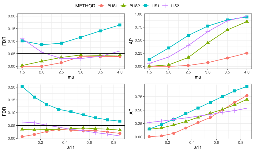
Figure 6: FDR and AP comparison when the HMM is misspecified. The null density $f_{0}$ is of $\mathcal{N}(0,1)$ and the signal’s density $f_{1}$ is of $\mathcal{N}(\mu,1)$.

E.2 HMMs with varying $\mu$

Consider the HMMs where $(\theta_{i})_{i=1}^{m}$ is a binary Markov chain with transition matrix $\mathbf{A}=(a_{ij})_{i,j=0,1}=(\mathbb{P}(\theta_{t+1}=j|\theta_{t}=i))_{i,j=0,1}$, where $a_{00}=0.95$ is fixed and the initial state of the latent chain is $\theta_{1}=0$. We fix $a_{11}$ and vary $\mu$. We apply $\rm PLIS_{HM}$, BH, AdaDetect, $\rm PLIS_{TG}$ and AdaPT to the simulated data. The simulation results are summarized in Figure 7.

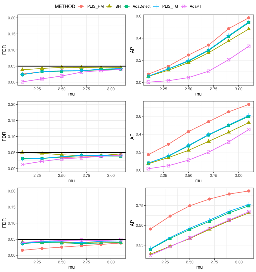
Figure 7: FDR and AP comparison for HMMs with varying $\mu$.

In Figure 7, the top, middle, and bottom rows correspond to different values of $a_{11}$ chosen from the set $\{0.3,0.5,0.8\}$, respectively. We observe that all the methods under consideration control the FDR at the nominal level. However, it is worth noting that the $\rm PLIS_{HM}$ procedure exhibits conservative in FDR levels across all simulation scenarios. Nonetheless it still has the highest average power among all the methods by effectively exploiting the structural patterns in the data.

E.3 More results on general dependence structures

In this section, we extend the discussion in Section 4.2 of the main text to include additional examples of structured multiple testing under different dependence structures. Notably, each of the three models considered here belongs to the class of structured probabilistic models (2), but deviates from the HMM in distinct ways. Despite these differences, all the models exhibit clustering patterns that can be approximated by HMMs to some extent. In practice, we employ the HMM as the working model to capture the underlying structural patterns and utilize the PLIS framework, which is guaranteed to make valid inference under the conditions specified in (2).

In the following, we describe the experimental setups for each of the three examples, summarize the results using figures, and finally draw observations and conclusions based on the patterns observed in the figures.

Example 1.

Heterogeneous HMMs. The setup is similar to that of Section E.2, which considers a conditional independence model with hidden states that follow a binary Markov chain: $X_{i}|\theta_{i}\overset{ind.}{\sim}(1-\theta_{i})\mathcal{N}(0,1)+\theta_{i}\mathcal{N}(\mu,1)$. However, we introduce a key modification by allowing the transition probability to vary over time. Specifically, we set $a_{11}^{(k)}=0.4\left(1+\sin\frac{k}{100}\right)$, where $k$ denotes the time index. This choice of transition probability results in a cyclical pattern in the data, which is often observed in meteorological analysis. In this context, signals tend to appear periodically, with varying patterns in the sizes of signal clusters. We apply PLIS ($\rm PLIS_{HM}$), BH and AdaDetect to the simulated data and summarize the results from 200 replications in Figure 8. ∎

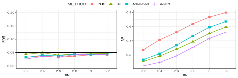
Figure 8: FDR and AP comparison when the model is a periodic heterogeneous HMM. Here $a_{11}^{(k)}=0.4\left(1+\sin\frac{k}{100}\right)$.

Example 2.

Two-layer dynamic models. This example presents a complex scenario where it is not possible to characterize the hidden states $\boldsymbol{\Theta}=(\theta_{i})_{i=1}^{m}$ in a closed form using a set of parameters, as is the case with HMMs. Instead, the state sequence $\Theta$ is determined by another dynamic sequence $\mathbf{Z}=(Z_{t})_{t=1}^{m}$. In turn, the state sequence determines the distribution of each observation in $\mathbf{X}$. This model, which describes the relationship between two different sequences $\mathbf{Z}$ and $\mathbf{X}$, is particularly useful for extracting common trends across different datasets. We now describe the data generating process for this example. Let $(Z_{t})_{t=1}$ be an autoregressive moving average (ARMA) sequence satisfying

$$Z_{t}=c+Z_{t-1}-0.5Z_{t-2}+\varepsilon_{t}+0.1\varepsilon_{t-1},c>0,$$

where the innovation $\{\varepsilon_{t}\}$ are i.i.d. $\mathcal{N}(0,0.5^{2})$ variables, and the hidden states are generated according to $\theta_{i}=\mathbb{I}\{Z_{i}<0\}$. The observed data $X_{i}$ are generated according to the structured probabilistic model: $X_{i}|\theta_{i}\overset{ind.}{\sim}(1-\theta_{i})\mathcal{N}(0,1)+\theta_{i}\mathcal{N}(\mu,1)$. We apply PLIS, BH, and AdaDetect to the simulated data and summarize the results from 200 replications in Figure 9. In the top row, we fix $c=0.3$ and vary $\mu$, whereas in the bottom row, we fix $\mu=2.8$ and vary $c$. Note that the average power of different methods would decrease with increasing $c$, as a larger value of $c$ causes $\mathbf{Z}$ to move in the positive direction, leading to fewer non-null hypotheses. ∎

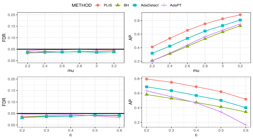
Figure 9: FDR and AP comparison under a two-layer dynamic model.

Example 3.

Structured models generated from a renewal process. The data in this example are generated in three steps based on a renewal process. First, we generate $Z_{i}$ using the following scheme:

$$Z_{i}\overset{i.i.d.}{\sim}Unif\{2,3,\cdots,20\} i=2k-1$$ for

$$Z_{i}\overset{i.i.d.}{\sim}Z Z-1\sim Poi(\lambda) i=2k$$ with for

where $k$ takes values of positive integers. Second, we generate $\theta_{j}$ as follows:

$$\theta_{j}=1 j\in[1+\sum_{i=1}^{K}Z_{i},\sum_{i=1}^{K+1}Z_{i}] K \theta_{j}=0$$ for if is odd, otherwise .

Finally, the observed data $X_{i}$ are generated according to the structured probabilistic model: $X_{i}|\theta_{i}\overset{ind.}{\sim}(1-\theta_{i})\mathcal{N}(0,1)+\theta_{i}\mathcal{N}(\mu,1)$. The length of the sequence is 2000. We apply PLIS, BH, and AdaDetect to the simulated data and summarize the results from 200 replications in Figure 10. In the top row, we fix $\lambda=2$ and vary $\mu$, whereas in the bottom row, we fix $\mu=2.8$ and vary $\lambda$. ∎

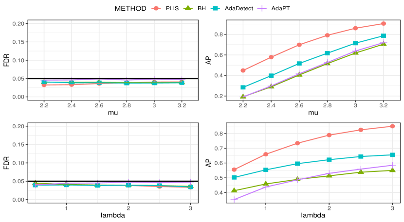
Figure 10: FDR and AP comparison in structured models generated from a renewal process.

It is worth noting that the three models discussed in this section pose significant challenges for analysis under the conventional “model-based” false discovery rate framework. In particular, this framework requires that the model be correctly specified, the model parameters be estimated consistently, and efficient algorithms be available to compute the conformity scores. However, due to the complexity of the models in above examples, meeting these requirements can be difficult, if not infeasible.

The results presented in Figures 7-10 are promising. They demonstrate that although the models cannot be estimated perfectly, it is still possible to use a working model to capture the structural patterns in the data and then employ the robust PLIS framework for inference. From the simulation results, we can see that the PLIS procedure remains valid across all setups. In terms of the ability to detect non-null signals, PLIS outperforms competing methods that employ symmetric rules by a substantial margin.

E.4 Numerical results for exchangeable data beyond Model (2)

This section reports on simulation studies conducted to compare different methods under the semi-supervised setup, where only labeled null samples are available without knowledge about the null distribution. We consider the situation where the observations are exchangeable but not conditionally independent given $\boldsymbol{\Theta}$. Specifically, the test data are generated using the following model:

$$X_{i}=\theta_{i}\mu+\varepsilon_{1,i}+\varepsilon_{2,i},\quad i\in[m],$$

where $\{\varepsilon_{1,i}\}$ are i.i.d. noise obeying $\mathcal{N}(0,1/2)$, and $\{\varepsilon_{2,i}\}$ are correlated noise with a marginal distribution of $\mathcal{N}(0,1/2)$, and a correlation of $corr(\varepsilon_{2,i},\varepsilon_{2,i^{\prime}})=\rho$ for $i\neq i^{\prime}$. The labeled null samples $\mathbf{U}=\{U_{i}\}$ are generated as follows:

$$U_{i}=\varepsilon_{1,m+i}+\varepsilon_{2,m+i},\quad i\in[2m].$$

In our simulation, we set $m=2000$, and the hidden binary variables $\boldsymbol{\Theta}=(\theta_{i})$ correspond to the hidden states in HMMs that represent the true states of the hypotheses.

Following the semi-supervised PLIS procedure (Algorithm 2), the first $m$ observations in $\mathbf{U}$ constitute the calibration set $\mathbf{Y}$, while the remaining data in $\mathbf{U}$ are used as training data. We compare the five methods at $\alpha=0.05$ under different settings, and obtain the FDR and AP levels by averaging the results from 200 replications. The simulation results are summarized in Figure 11, where we fix $a_{00}=0.95$, $a_{11}=0.8$, and $\rho=0.4$, and vary $\mu$ in the top row. In the middle and bottom rows, we set $a_{11}=0.8$ and $a_{11}=0.5$, respectively, and compare the different methods for varying values of $\rho$.

The results in Figure 11 show that $\rm PLIS_{HM}$, $\rm PLIS_{TG}$, and AdaDetect effectively control the FDR at the nominal level in all settings. However, AdaPT shows inflated FDR levels. The proposed method $\rm PLIS_{HM}$ displays the highest average power among all the methods.

Figure 11: FDR and AP comparison when data points are exchangeable under the null but not independent conditional on $\boldsymbol{\Theta}$.

E.5 Numerical results for non-exchangeable data

In this section, we conduct numerical studies to evaluate the performance of the semi-supervised PLIS method (Algorithm 2) when the exchangeability assumption is violated. This situation is of particular interest as it is difficult to establish rigorous theoretical guarantees on FDR control. The test data are generated using the following model:

$$X_{i}=\theta_{i}\mu+\varepsilon_{1,i}+\varepsilon_{2,i},\quad i\in[m].$$

The labeled null samples $\mathbf{U}=\{U_{i}\}$ are generated as follows:

$$U_{i}=\varepsilon_{1,m+i}+\varepsilon_{2,m+i},\quad i\in[2m],$$

where $\{\varepsilon_{1,i}\}$ are i.i.d. noise obeying $\mathcal{N}(0,1/2)$, and $\{\varepsilon_{2,i}\}$ are correlated noise with a marginal distribution given by $\mathcal{N}(0,1/2)$. The correlation structure can be described as an auto-regressive model [AR(1)], i.e., the correlation coefficient is given by $\mathbb{E}[\varepsilon_{2,i}\varepsilon_{2,j}]=\rho^{|i-j|}$ for some $\rho\neq 0$. As before, we set $m=2000$, and the hidden binary variables $\boldsymbol{\Theta}=(\theta_{i})$ correspond to the hidden states in HMMs that represent the true states of the hypotheses.

We compare the previously mentioned methods at $\alpha=0.05$ under different settings and obtain the FDR and AP levels by averaging the results from 200 replications. The simulation results are summarized in Figure 12, where in the top row, we fix $a_{00}=0.95$, $a_{11}=0.8$, and $\rho=0.5$, and vary $\mu$. In the bottom row, we set $a_{11}=0.8$ and $\mu=2.8$ and compare the different methods for varying values of $\rho$.

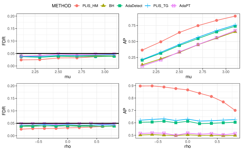
Figure 12: FDR and AP comparison for nonexchangeable data with AR(1) structure.

The numerical results demonstrate that although it is difficult to establish a theoretical guarantee for PLIS when the null data are not exchangeable, the FDR can be effectively controlled under the nominal level. Compared to the results presented in Figure 11, the performance of BH, AdaDetect, $\rm PLIS_{TG}$, and AdaPT is robust against the violation of exchangeability assumption when there is an AR(1) dependence structure. This may be attributed to the weakly dependent nature of the AR(1) process, wherein the correlation coefficient decreases exponentially. The other possible explanation is that the AR(1) Gaussian process belongs to the $\alpha$-mixing processes; the kernel density estimators employed by AdaDetect and $\rm PLIS_{TG}$ are consistent under such mixing conditions.

E.6 Derandomized PLIS

In this section, we investigate issues related to Derandomized PLIS, which involves averaging multiple mirror processes/e-values. A critical aspect is the effective selection of hyper-parameters, including the number of replicates $N$ and the FDR levels for every realized PLIS: $(\alpha_{j})_{j=1}^{N}$. This remains an open question that goes beyond the scope of this work. We provide some preliminary results for Derandomized PLIS with some pairs of $(N,\alpha_{PLIS})$, which are presented in Table 1. We set $\alpha_{PLIS}$ to be proportional to the target FDR level $\alpha=0.05$ and choose $\alpha_{1}=\cdots=\alpha_{N}\equiv\alpha_{PLIS}$.

In our numerical study, we generate the data using the two-group model (3), which is also utilized as the working model for PLIS:

$$X_{i}|\theta_{i}\overset{ind.}{\sim}(1-\theta_{i})\mathcal{N}(0,1)+\theta_{i}\mathcal{N}(\mu,1),$$

where $\theta_{1},\cdots,\theta_{m}$ are i.i.d. binary variables, $\mathbb{P}(\theta_{1}=1)=\pi$. The density ratio (DR) statistic serves as an ideal score function. We compare the above methods on simulated data by fixing $\pi=0.2$. The average results from 200 replications are displayed in Figure 13.

Figure 13 presents the comparison results for Derandomized PLIS with different hyper-parameters. It is observed that all methods are valid for FDR control, as supported by the theory of the e-BH procedure, which is employed as the final step to determine the rejections in Derandomized PLIS. Notably, the highest power is achieved when $\alpha_{PLIS}=0.5\alpha$, while no discovery is made when $\alpha_{PLIS}=1.2\alpha$. By contrast, the multiplication parameter $N$ has little effect on the performance of Derandomized PLIS procedure.

Table 1: Methods corresponding to the pair of hyper-parameters in the experiment for Derandomized PLIS.

METHOD	$\alpha_{PLIS}=\alpha$	$\alpha_{PLIS}=0.5\alpha$	$\alpha_{PLIS}=1.2\alpha$
$N=60$	N60_a	N60_0.5a	N60_1.2a
$N=30$	N30_a	N30_0.5a	N30_1.2a

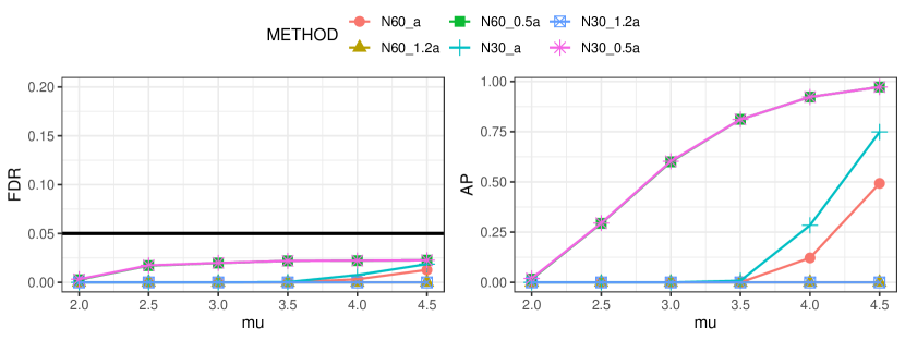
Figure 13: This figure compares the FDR and AP for the mixture model (3) with varying $\mu$, while controlling the FDR level at $\alpha=0.05$. The experiment fixes $\pi=0.2$, and all implemented methods are Derandomized PLIS with different hyper-parameters (Table 1).

As highlighted by Ren and Barber (2023), it is intuitively preferable to choose $\alpha_{PLIS}$ to be less than $\alpha$ when the sample size $N>1$. To illustrate this, consider a scenario where the data contains $m_{1}$ non-nulls, each exhibiting remarkably strong signals, resulting in the high likelihood of selecting all $m_{1}$ non-nulls in a single run of PLIS. In each run $j$, we would anticipate an approximate false discovery proportion of $\alpha_{PLIS}$. This implies that we would expect to observe around $\frac{\alpha_{PLIS}}{1-\alpha_{PLIS}}m_{1}$ false discoveries along with the $m_{1}$ true discoveries. Since each non-null $i$ is selected in nearly every run of PLIS, while it is possible for a null $k\in\mathcal{H}_{0}$ to be chosen only in a small proportion of the runs, we would expect the e-values to behave as $e_{j}\approx m/(\frac{\alpha_{PLIS}}{1-\alpha_{PLIS}}m_{1})$ for $j\notin\mathcal{H}_{0}$, and approximately $e_{j}\approx 0$ for $j\in\mathcal{H}_{0}$.

Applying the e-BH procedure at level $\alpha$ to these e-values, we observe that the power of the procedure can be high only if $m/(\frac{\alpha_{PLIS}}{1-\alpha_{PLIS}}m_{1})\geq m/(\alpha m_{1})$. Otherwise, if this condition is not met, the power will be zero, as no discoveries can be made. Consequently, selecting $\alpha_{PLIS}\leq\frac{\alpha}{1+\alpha}$ may result in a powerful procedure. However, it is important to note that our examination of the relationship between the $\alpha_{k}$s and $\alpha$ is still at a preliminary stage and has not reached a conclusive point. We believe that further investigation into this topic is warranted.

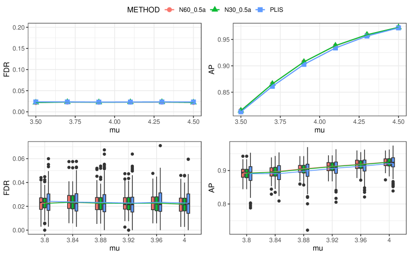
Figure 14: Comparison for Derandomized PLIS with $\alpha_{k}=0.5$ and PLIS. The top row is the line chart representing the trends of FDR and AP for varying $\mu$, while the bottom row is the boxplots for comparison.

To demonstrate the effectiveness of derandomization, we compare the FDR and AP levels between PLIS and Derandomized PLIS, utilizing a mixture model (3) with a mixing proportion of $\pi=0.2$. The nominal FDR level is set at $\alpha=0.05$. A summary of the simulation results is presented in Figure 14. It becomes apparent that employing Derandomized PLIS with $\alpha_{k}=0.5\alpha$ yields improvement in power. Furthermore, the boxplots displayed in the bottom row of the figure visually reinforce the notion that derandomization effectively reduces both the variance and number of outliers. As a result, derandomization provides a useful tool for enhancing the replicability and reliability of the discoveries made.

E.7 Comparison for different baseline data constructions in PLIS

In this section, we provide numerical results to compare the efficacy of different baseline data construction methods. The pairwise exchangeability properties (Properties 1-3) hold as long as the bivariate function is symmetric, i.e., $h(x,y)=h(y,x)$. Among the baseline data construction methods, we recommended using the function

$$h(x,y)=\left\{\begin{matrix}x&\text{if $|x|\geq|y|$}\\ y&\text{otherwise}\end{matrix}\right..$$

This choice of function provides two significant benefits. First, it guarantees pairwise exchangeability, which our theoretical analysis requires. Second, it maintains large non-null effects and hence essential structural information. However, alternative functions such as $h^{\prime}(x,y)=x+y$ also guarantee pairwise exchangeability and can lead to a valid PLIS procedure.

We demonstrate that using alternative functions, such as $h(x,y)=x+y$, can lead to a dilution of non-null effects in the test data, thereby decreasing the power of the PLIS procedure. Denote the PLIS procedure with $h^{\prime}(x,y)=x+y$ as PLIS.2. We generate test data using the process

$$X_{i}|\theta_{i}\overset{ind.}{\sim}(1-\theta_{i})\mathcal{N}(0,1)+\theta_{i}\mathcal{N}(0,1),i\in[m],$$

with $m=2000$. The calibration data $Y_{1},\cdots,Y_{m}$ are i.i.d. $\mathcal{N}$(0,1).

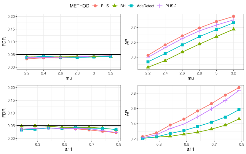
Figure 15: FDR and AP comparison for PLIS with different baseline data constructions.

We consider two simulation setups. In the first setup, the underlying states $\boldsymbol{\Theta}$ are generated from a two-layer model. Specifically, let $(Z_{t})_{t=1}$ be an autoregressive moving average (ARMA) sequence satisfying $Z_{t}=0.4+Z_{t-1}-0.5Z_{t-2}+\varepsilon_{t}+0.1\varepsilon_{t-1}$, where the innovations $\{\varepsilon_{t}\}$ are i.i.d. $\mathcal{N}(0,0.5^{2})$ variables, and the hidden states are generated according to $\theta_{i}=\mathbb{I}\{Z_{i}<0\}$. In the second setup, the hidden states $\boldsymbol{\Theta}=(\theta_{i})$ are generated as a Markov chain with $a_{00}=0.95$, $\mu=2.6$, and varying $a_{11}$.

We apply various methods to the simulated data at FDR level $\alpha=0.05$. The simulation results for the two setups are summarized in the first and second rows of Figure 15, respectively. We can see that PLIS.2 control the FDR at the nominal level and outperforms BH and AdaDetect in power. However, PLIS.2 is not as efficient as the proposed PLIS in terms of power. This corroborates the merits of the proposed bivariate function employed for construction of the baseline data in our paper.

References

- Barber and Candès (2015) Barber, R. F. and E. J. Candès (2015). Controlling the false discovery rate via knockoffs. The Annals of Statistics 43(5), 2055 – 2085.
- Barber et al. (2023) Barber, R. F., E. J. Candes, A. Ramdas, and R. J. Tibshirani (2023). De finetti’s theorem and related results for infinite weighted exchangeable sequences. arXiv preprint arXiv:2304.03927.
- Barrett et al. (2009) Barrett, J. C., D. G. Clayton, P. Concannon, B. Akolkar, J. D. Cooper, H. A. Erlich, C. Julier, G. Morahan, J. Nerup, C. Nierras, et al. (2009). Genome-wide association study and meta-analysis find that over 40 loci affect risk of type 1 diabetes. Nature genetics 41(6), 703–707.
- Bashari et al. (2023) Bashari, M., A. Epstein, Y. Romano, and M. Sesia (2023). Derandomized novelty detection with fdr control via conformal e-values. arXiv preprint arXiv:2302.07294.
- Bates et al. (2023) Bates, S., E. Candès, L. Lei, Y. Romano, and M. Sesia (2023). Testing for outliers with conformal p-values. The Annals of Statistics 51(1), 149 – 178.
- Benjamini and Heller (2007) Benjamini, Y. and R. Heller (2007). False discovery rates for spatial signals. Journal of the American Statistical Association 102(480), 1272–1281.
- Benjamini and Hochberg (1995) Benjamini, Y. and Y. Hochberg (1995). Controlling the false discovery rate: a practical and powerful approach to multiple testing. Journal of the Royal statistical society: series B (Methodological) 57(1), 289–300.
- Benjamini and Yekutieli (2001) Benjamini, Y. and D. Yekutieli (2001). The control of the false discovery rate in multiple testing under dependency. The Annals of Statistics 29(4), 1165–1188.
- Candès et al. (2018) Candès, E., Y. Fan, L. Janson, and J. Lv (2018). Panning for gold: ‘model-x’ knockoffs for high dimensional controlled variable selection. Journal of the Royal Statistical Society: Series B (Statistical Methodology) 80(3), 551–577.
- Copas (1974) Copas, J. B. (1974). On symmetric compound decision rules for dichotomies. Annals of Statistics 2(1), 199–204.
- Diaconis and Freedman (1980) Diaconis, P. and D. Freedman (1980). Finite Exchangeable Sequences. The Annals of Probability 8(4), 745 – 764.
- Du et al. (2023) Du, L., X. Guo, W. Sun, and C. Zou (2023). False discovery rate control under general dependence by symmetrized data aggregation. Journal of the American Statistical Association 118(541), 607–621.
- Durrett (2019) Durrett, R. (2019). Probability: theory and examples, Volume 49. Cambridge university press.
- Efron et al. (2001) Efron, B., R. Tibshirani, J. D. Storey, and V. Tusher (2001). Empirical bayes analysis of a microarray experiment. Journal of the American statistical association 96(456), 1151–1160.
- Fan et al. (2012) Fan, J., X. Han, and W. Gu (2012). Estimating false discovery proportion under arbitrary covariance dependence. Journal of the American Statistical Association 107(499), 1019–1035.
- Goodfellow et al. (2016) Goodfellow, I., Y. Bengio, and A. Courville (2016). Deep Learning. MIT Press. http://www.deeplearningbook.org.
- Grünwald et al. (2020) Grünwald, P., R. de Heide, and W. M. Koolen (2020). Safe testing. In 2020 Information Theory and Applications Workshop (ITA), pp. 1–54. IEEE.
- Guan (2014) Guan, Y. (2014, 03). Detecting Structure of Haplotypes and Local Ancestry. Genetics 196(3), 625–642.
- Heath and Sudderth (1976) Heath, D. and W. Sudderth (1976). De finetti’s theorem on exchangeable variables. The American Statistician 30(4), 188–189.
- Ignatiadis and Huber (2021) Ignatiadis, N. and W. Huber (2021). Covariate Powered Cross-Weighted Multiple Testing. Journal of the Royal Statistical Society Series B: Statistical Methodology 83(4), 720–751.
- Lafferty et al. (2001) Lafferty, J. D., A. McCallum, and F. C. N. Pereira (2001). Conditional random fields: Probabilistic models for segmenting and labeling sequence data. In Proceedings of the Eighteenth International Conference on Machine Learning, ICML ’01, San Francisco, CA, USA, pp. 282–289. Morgan Kaufmann Publishers Inc.
- Lei and Fithian (2018) Lei, L. and W. Fithian (2018). AdaPT: An Interactive Procedure for Multiple Testing with Side Information. Journal of the Royal Statistical Society Series B: Statistical Methodology 80(4), 649–679.
- Liang and Nettleton (2010) Liang, K. and D. Nettleton (2010). A hidden markov model approach to testing multiple hypotheses on a tree-transformed gene ontology graph. Journal of the American Statistical Association 105(492), 1444–1454.
- Liang et al. (2022) Liang, Z., M. Sesia, and W. Sun (2022). Integrative conformal p-values for powerful out-of-distribution testing with labeled outliers. arXiv preprint arXiv:2208.11111.
- Liu et al. (2016) Liu, J., C. Zhang, and D. Page (2016). Multiple testing under dependence via graphical models. The Annals of Applied Statistics 10(3), 1699 – 1724.
- Marandon et al. (2022) Marandon, A., L. Lei, D. Mary, and E. Roquain (2022). Machine learning meets false discovery rate. arXiv preprint arXiv: 2208.06685.
- Mary and Roquain (2022) Mary, D. and E. Roquain (2022). Semi-supervised multiple testing. Electronic Journal of Statistics 16(2), 4926–4981.
- Onsager (1944) Onsager, L. (1944). Crystal statistics. i. a two-dimensional model with an order-disorder transition. Physical Review 65(3-4), 117–149.
- Perrot-Dockès et al. (2021) Perrot-Dockès, M., G. Blanchard, P. Neuvial, and E. Roquain (2021). Post hoc false discovery proportion inference under a hidden markov model. arXiv preprint arXiv:2105.00288.
- Rabiner (1989) Rabiner, L. (1989). A tutorial on hidden markov models and selected applications in speech recognition. Proceedings of the IEEE 77(2), 257–286.
- Rebafka et al. (2022) Rebafka, T., É. Roquain, and F. Villers (2022). Powerful multiple testing of paired null hypotheses using a latent graph model. Electronic Journal of Statistics 16(1), 2796 – 2858.
- Ren and Barber (2023) Ren, Z. and R. F. Barber (2023). Derandomized knockoffs: leveraging e-values for false discovery rate control. arXiv preprint arXiv:2205.15461.
- Ren and Candès (2023) Ren, Z. and E. Candès (2023). Knockoffs with side information. The Annals of Applied Statistics 17(2), 1152 – 1174.
- Sarkar (2002) Sarkar, S. K. (2002). Some results on false discovery rate in stepwise multiple testing procedures. The Annals of Statistics 30(1), 239–257.
- Schervish (2012) Schervish, M. J. (2012). Theory of statistics. Springer Science & Business Media.
- Sesia et al. (2018) Sesia, M., C. Sabatti, and E. J. Candès (2018, 08). Gene hunting with hidden Markov model knockoffs. Biometrika 106(1), 1–18.
- Shafer (2021) Shafer, G. (2021). Testing by betting: A strategy for statistical and scientific communication. Journal of the Royal Statistical Society: Series A (Statistics in Society) 184(2), 407–431.
- Shu et al. (2015) Shu, H., B. Nan, and R. Koeppe (2015). Multiple testing for neuroimaging via hidden markov random field. Biometrics 71(3), 741–750.
- Storey (2003) Storey, J. D. (2003). The positive false discovery rate: a Bayesian interpretation and the q-value. The Annals of Statistics 31(6), 2013 – 2035.
- Sun and Cai (2007) Sun, W. and T. T. Cai (2007). Oracle and adaptive compound decision rules for false discovery rate control. Journal of the American Statistical Association 102(479), 901–912.
- Sun and Cai (2009) Sun, W. and T. T. Cai (2009). Large-scale multiple testing under dependence. Journal of the Royal Statistical Society: Series B (Statistical Methodology) 71(2), 393–424.
- Sun et al. (2015) Sun, W., B. J. Reich, T. T. Cai, M. Guindani, and A. Schwartzman (2015). False discovery control in large-scale spatial multiple testing. Journal of the Royal Statistical Society. Series B, Statistical methodology 77(1), 59.
- Vovk et al. (2005) Vovk, V., A. Gammerman, and G. Shafer (2005). Algorithmic learning in a random world, Volume 29. Springer.
- Vovk and Wang (2021) Vovk, V. and R. Wang (2021). E-values: Calibration, combination and applications. The Annals of Statistics 49(3), 1736–1754.
- Wang and Ramdas (2022) Wang, R. and A. Ramdas (2022). False discovery rate control with e-values. Journal of the Royal Statistical Society: Series B (Statistical Methodology) 84(3), 822–852.
- Wei et al. (2009) Wei, Z., W. Sun, K. Wang, and H. Hakonarson (2009). Multiple testing in genome-wide association studies via hidden markov models. Bioinformatics 25(21), 2802–2808.
- Weinstein et al. (2017) Weinstein, A., R. Barber, and E. Candes (2017). A power and prediction analysis for knockoffs with lasso statistics. arXiv preprint arXiv:1712.06465.
- Wu (2008) Wu, W. B. (2008). On false discovery control under dependence. The Annals of Statistics 36(1), 364 – 380.
- Yang et al. (2021) Yang, C.-Y., L. Lei, N. Ho, and W. Fithian (2021). Bonus: Multiple multivariate testing with a data-adaptivetest statistic. arXiv preprint arXiv:2106.15743.