Noise robustness of a multiparty quantum summation protocol

Abstract

Connecting quantum computers to a quantum network opens a wide array of new applications, such as securely performing computations on distributed data sets. Near-term quantum networks are noisy, however, and hence correctness and security of protocols are not guaranteed. To study the impact of noise, we consider a multiparty summation protocol with imperfect shared entangled states. We study analytically the impact of both depolarising and dephasing noise on this protocol and the noise patterns arising in the probability distributions. We conclude by eliminating the need for a trusted third party in the protocol using Shamir’s secret sharing.

1 Introduction

Quantum computing is an emerging field where advances are made on the hardware-side, software-side, as well as applications. Many companies and universities are working on building better quantum hardware with more resources of better quality. At the same time, new algorithms are being discovered, and these new quantum algorithms are applied in various new settings.

The theoretical speedup quantum computers offer for various problems discerns them from classical alternatives. Amongst these are some of the most complicated problems encountered in every-day life. Examples where quantum computers outperform classical alternatives include breaking certain asymmetric encryption protocols [1, 2], developing new materials and personalised medicines [3], and solving complex systems of linear equations [4].

Another aspect at which quantum computers distinguish themselves from classical alternatives, is the security of a quantum state: Opposed to classical information, in general, quantum information cannot be read out or copied faithfully. Reading out a quantum state will destroy the state irrevocably and information will be lost, whereas trying to copy a quantum state leaves the state and its copy entangled, and operations performed on an entangled copy differ from those applied to the original unentangled state. Because of this, sharing information via quantum states remains secure. This idea underlies the field of quantum communication and its subfield quantum key distribution.

Combining quantum computing with quantum communication joins the best of both worlds: by using quantum communication between different quantum computers, these devices can collaboratively solve larger problems, while the information shared between the devices remains secure. This field is called Distributed Quantum Computing (DQC).

Eisert et al. gave the first description of how to perform operations between different quantum devices through the use of quantum communication [5]. Later, this work was extended and a distributed version of Shor’s algorithm was theorised [6, 7]. Distributed quantum computing works by transforming traditional quantum algorithms to their distributed version. In these distributed versions, operations performed between qubits located on different devices are called non-local and are replaced by a non-local quantum gate established using shared entangled states. In comparison, operations between qubits on the same device are called local, and are unchanged from the traditional algorithm to the distributed one. These three works consider all operations, both local and non-local, to be perfect. Beals et al. later proved that distributing an algorithm over different resources incurs only a small overhead in the cost [8]. Hence, when programming quantum algorithms on a higher level, the underlying structure of the hardware, local or distributed, has only a marginal effect.

Follow-up work mainly focused on applications run using a distributed quantum network [9], or on how to best implement a distributed quantum computer network [10, 11]. One aspect to take into account in these distributed networks is the robustness against noise, as current hardware is noisy and will remain so for the foreseeable future. It is therefore interesting to consider the effect of imperfect operations in such distributed settings. A first work on this topic computed the fidelity of a distributed and imperfect quantum phase estimation algorithm, when distributed over a varying number of devices [12]. Another example is the work by Khabiboulline et al. where a secure quantum voting protocol is presented [13]

In this work, we extend this line of research by again considering imperfect non-local operations, but now applied to a multiparty summation protocol. In this protocol, we consider different parties which aim to compute the sum of their inputs, without revealing these inputs. Each party has access to a local quantum computer, which can generate shared entangled states with other devices. We then consider how dephasing and depolarising noise on the shared entangled states affects the output fidelity of this distributed summation protocol.

Section 2 explains both the multiparty summation protocol and the two considered noise models. Next, Section 3 presents the results of our simulations for both noise models. Section 4 contains an analytical study of observed noise patterns and the periodicity therein. Afterwards, Section 5 details how the algorithm can be extended in such a way that each party learns the output, without revealing the individual inputs to the other parties. Section 6 concludes with a summary and an outlook to future work in the direction of distributed quantum computing.

2 Preliminaries

2.1 Distributed Quantum Computing

Distributed quantum computing entails the collaborative execution of quantum algorithms using multiple quantum devices. Distributed computations can occur at various levels: for example, the devices may independently run their own quantum circuits, after which the outputs are combined to obtain the final results. Alternatively, the devices may cooperate intricately through quantum communication to execute a single overall circuit. This study concentrates on the latter scenario, specifically exploring the execution of a distributed quantum addition circuit.

The key challenge in this form of distributed quantum computing, is the application of non-local multi-qubit gates. As any multi-qubit gate can be decomposed into CNOT gates with additional local one-qubit gates [14], it suffices to implement the CNOT-gates in a non-local fashion. Figure 1 shows an implementation of a non-local CNOT gate between the states $\ket{\phi}$ and $\ket{\psi}$ located on different devices. The protocol requires shared entanglement between the two devices in the form of a $GHZ_{2}$ state. The procedure involves two gates conditioned by a measurement outcome obtained by the other party. Classical communication is thus needed between the parties in order to implement the non-local CNOT. By decomposing and replacing every CNOT by a non-local CNOT, any quantum circuit can be ran in a distributed manner.

${\Qcircuit@C=1em@R=0.7em{\lstick{\ket{\phi}}&\qw\ctrl{1}\qw\qw\qw\qw\qw\gate{Z}\qw\\ \ghost{GHZ_{2}}\targ\meter\control\cw\cwx[1]\\ \multigate{-1}{GHZ_{2}}\qw\qw\targ\ctrl{1}\gate{H}\meter\control\cw\cwx[-2]\\ \lstick{\ket{\psi}}\qw\qw\qw\qw\targ\qw\qw\qw\qw}}$

Figure 1: Quantum circuit for a non-local CNOT-gate between $\ket{\phi}$ and $\ket{\psi}$ located on different devices that share a GHZ-state. Double lines denote classical information.

In this work we consider the distributed quantum summation protocol [15], which extends the quantum summation algorithm proposed by Draper [16] and later improved by Ruiz-Perez [17]. The quantum summation algorithm uses the Quantum Fourier Transform to map the states to their phase state representation. In the phase space, addition corresponds to specific controlled phase gates. We start by describing the non-distributed version, after which we explain the distributed version.

Suppose we have two integers $a,b<2^{n}$ that we wish to add and that we have the two quantum states $\ket{a}$ and $\ket{b}$ using the binary representation of the integers using $n$ qubits. The protocol first applies the quantum Fourier transform of size $n$, denoted by $QFT_{n}$ to $\ket{b}$. This yields the phase state representation of $b$, given by $\ket{\phi(b)}$. Then, applying phase gates to the qubits of $\ket{\phi(b)}$ controlled by the qubits of $\ket{a}$ gives the quantum state $\ket{\phi(a+b)}$. An inverse quantum Fourier transform the gives the original state $\ket{a+b}$ again. Figure 2 gives a schematic overview of the phase gates of this protocol $n=3$ qubits. We omitted the two Fourier transforms.

@C=1em @R=0.7em —a_0⟩ & 3 4 5 —a_0⟩

—a_1⟩

3 4 —a_1⟩

—a_2⟩

3 —a_2⟩

—ϕ(b)_0⟩

π/2 —ϕ(b+a)_0⟩

—ϕ(b)_1⟩

π/4 π/2 —ϕ(b+a)_1⟩

—ϕ(b)_2⟩

π/8 π/4 π/2 —ϕ(b+a)_2⟩

Figure 2: The addition part of a quantum summation circuit. The state $\ket{\phi(b)_{j}}$ represents the $j$-th bit of the Quantum Fourier transform of $b$. The blocks represent controlled-$R_{Z}$ gates, where the argument shown is the angle used by the $R_{Z}$-gate. An inverse quantum Fourier transform on the second half of the register gives the quantum state $\ket{a}\ket{b+a}$.

This summation protocol can easily be extended to allow a server party to do the addition of $k$ different numbers held by $k$ different computing parties. Figure 3 gives the extended protocol with an additional server party. The server party holds the result at the end of the protocol. Note that the phase gates applied by different parties commute and hence, every party can apply their local phase gates simultaneously.

@C=0.5em @R=0.45em s:—0⟩ & 2QFT 3 3 2QFT^-1

s:—0⟩ QFT 3 3 QFT^-1

s:—0⟩ QFT 3 3 QFT^-1

p_1:—0⟩ [3] 2Add x^1 [3] —0⟩

p_1:—0⟩ [3] Add x^1 [3] —0⟩

p_1:—0⟩ [3] Add x^1 [3] —0⟩

p_2:—0⟩ 2Add x^2 —0⟩

p_2:—0⟩ Add x^2 —0⟩

p_2:—0⟩ Add x^2 —0⟩

Figure 3: Example of DISTRIBUTED-QFT-ADDER [15]. A server party adds integers from two computing parties. The blocks $\text{Add }x^{k}$ denote the phase-gates needed to add integer $x^{k}$, similar to Figure 2. The final quantum state in the first register is $\ket{x^{1}+x^{2}}$.

The above multi-party protocol translates to a non-local protocol by replacing every CNOT gate by a non-local CNOT gate. The resulting protocol is called the DISTRIBUTED-QFT-ADDER. Multiple implementations for the CNOT-gates exist, some of which even allow simultaneous implementation of the phase gates by all parties [15].

2.2 Noise models

The work by Neumann and Wezeman ignores the presence of noise in the systems. In practice, at least for the near-term, quantum hardware remains noisy and it is necessary to consider decoherence effects when developing applications. Currently, the fidelity of state teleportation between non neighbouring nodes is around $0.7$ [18] and the fidelity of quantum operations on quantum devices is around $0.95$ to $0.99$ [19]. For this reason, we omit in this work the effect of imperfect quantum operations, and only consider an imperfect quantum network.

The quantum network distributes entangled $GHZ$ states between different the server node and the nodes of the different parties. The presence of noise translates to having imperfect entanglement between the nodes.

Current state-of-the-art protocols for entanglement generation between nodes of a quantum network are heralded, which allows to deterministically know whether the entanglement distribution process succeeded. Typically, heralding work in experiments via a photon measurement such that entanglement is established if and only if a photon has been detected. We therefore disregard lossy quantum channels by assuming that the distribution is done in a heralded way.

In this study, we consider two types of noise in the quantum links, namely dephasing and depolarising noise. These types of noise arise often in physical implementations and current software packages allow for easy simulation of these noise type, whilst the analytic study remains feasible at the same time. The respective noise channels are applied to the quantum links by applying them to all qubits in the $GHZ$ state independently.

2.2.1 Noise model A: Dephasing channel

A dephasing channel is a completely positive and trace-preserving (CPTP) map that represents the decay of the quantum phase of a system, that is, the off-diagonal elements of the density matrix. A one-qubit dephasing channel $\varepsilon_{depha}$ is usually represented by the map

$$\varepsilon_{depha}:\rho\mapsto\left(1-\frac{p}{2}\right)\rho+\frac{p}{2}\mathbf{Z}\rho\mathbf{Z}$$ (1)

which leaves the state unchanged with probability $1-p/2$ and performs a phase flip with probability $p/2$. Writing the matrix representation of this channel we see, indeed, that it corresponds to a phase damping process:

$$\rho=\begin{pmatrix}\rho_{00}&\rho_{01}\\ \rho_{10}&\rho_{11}\end{pmatrix}\rightarrow\varepsilon_{depha}(\rho)=\begin{pmatrix}\rho_{00}&(1-p)\rho_{01}\\ (1-p)\rho_{10}&\rho_{11}\end{pmatrix}.$$ (2)

Dephasing errors can arise in fiber optic links due to a phenomenon called birefringence, which is associated with changes in the refractive index for different polarisations or different regions of the material [20]. In fact, using a special polarisation maintaining optical fiber, the decoherence in these links can be completely described via dephasing processes [21]. Assuming heralded entanglement distribution, we can ignore the high attenuation arising in fiber optic links. Our focus is the impact of noise on the fidelity of the protocol, so we omit the entanglement generation rate and the lower transmission rates.

2.2.2 Noise model B: Depolarising channel

The depolarising channel is usually seen as the quantum equivalent of white noise. Depolarising channels model processes that completely scramble the starting state with a some probability. As a result, both quantum and classical information is lost. Given a valid $n$-qubit quantum state $\rho$, an $n$-qubit depolarising channel $\varepsilon_{depol}$ can be written as

$$\varepsilon_{depol}:\rho\mapsto(1-p)\rho+\frac{p}{d}\mathbf{I},$$ (3)

where $d=2^{n}$ is the dimension of the Hilbert space $\rho$ lives in.

Depolarising channels can, amongst other things, model the misalignment of reference frames between the nodes in a quantum network [22]. Moreover, depolarising channels can also model what happens if heralding fails, for instance when the detector wrongfully measures a photon. Such an event is called a dark count and leads to reading out an empty quantum memory [23].

3 Simulations with noise

We simulated the quantum summation protocol [15] and included the noise models discussed above to see how well the protocols still perform in noisy settings. By adding dephasing and/or depolarising noise to the protocol, we expect incorrect outcomes found by the server party at the end of the protocol. Therefore, we report the results as probability distributions in histograms or equivalent polar plots.

We implemented both noise models using Qiskit [24] and only applied the noise models to the quantum links. So we apply a noise channel to the generated $GHZ$-states. We implemented these noise models by inserting local noisy identity gates at the end of the $GHZ$ generation block. We ran experiments for varying number of parties and inputs, as well as noise levels. Each simulation consists on $9{,}000$ independent runs of the circuit.

3.1 Dephasing noise

We first consider the impact of the dephasing noise by analysing four parties, each with input $1$ and a dephasing noise of $p/2=0.07$ for each of the four quantum links. Figure 4 shows the resulting probability distribution in blue and the ideal (noiseless) probability distribution in red.

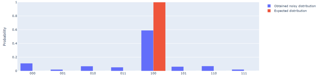
Figure 4: Distribution of outcomes for the case of four parties inputting $1$, and a dephasing noise of $p/2=0.07$ applied on each entangled qubit pair. The correct outcome is given by $100$ in binary.

In the noisy setting, the correct outcome, $4$ or $100$ in binary, has the highest probability, followed by outcome $000$. The probability distribution seems to have some symmetry (cf. Section 4), hence Figure 5 shows the probability distribution in a polar plot. The second most frequent outcome is diametrically opposed to the correct one; and the next two most frequent outcomes are $\pi/2$ radians away from the highest probability and diametrically opposed to each other.

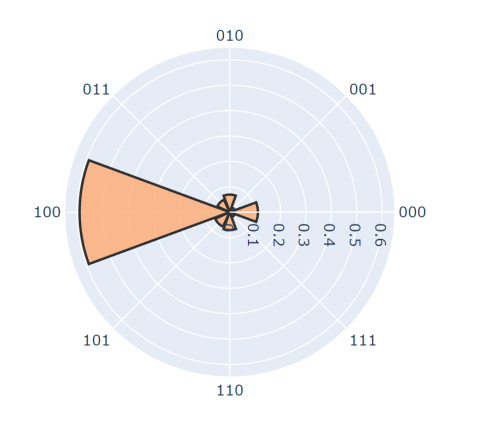
Figure 5: Polar representation of the distribution shown in Figure 4.

Interestingly, this symmetry emerges also for a different number of parties and for varying inputs. First, Figure 6 shows the results for the same number of parties and inputs but with different levels of noise. Even though the output distribution approaches a uniform distribution with increasing noise levels $p$, the symmetry in the probability distribution is preserved. Second, Figure 7 shows the results for a protocol run with two parties, both of them inputting $2$, for varying values of $p$. Again, a similar noise pattern emerges, indicating that the noise pattern is independent of the number of parties involved. Finally, Figure 8 shows the results for a protocol run with two parties, where one of them inputs $10$ and the other $7$, again for varying values of $p$. We again see similar symmetries appearing in the noise probability distribution, which indicates that the probability distribution is independent of the input values of the parties.

Four parties, dephasing noise

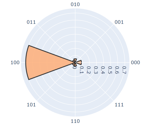
(a) $p/2=0.05$

(b) $p/2=0.25$

Figure 6: Probability distribution for the case of four parties inputting $1$, with identical dephasing noise applied on each entangled qubit pair for varying noise levels, $p/2$, as indicated. The correct outcome is given by $100$ in binary.

Two parties, dephasing noise

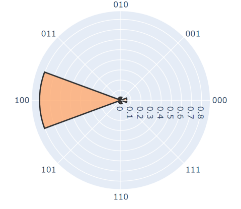
(a) $p/2=0.05$

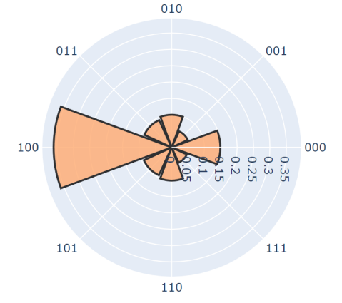
(b) $p/2=0.25$

Figure 7: Probability distribution for the case of two parties inputting $2$, with identical dephasing noise applied on each entangled qubit pair for varying noise levels, $p/2$, as indicated. The correct outcome is given by $100$ in binary.

Two parties, dephasing noise

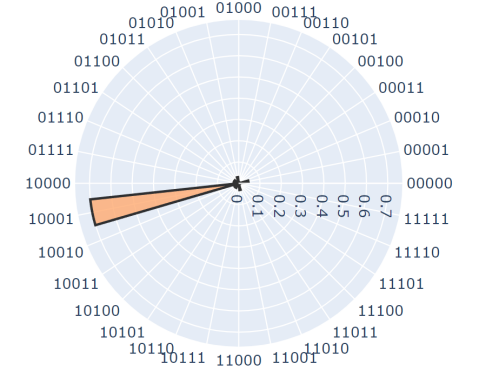
(a) $p/2=0.05$

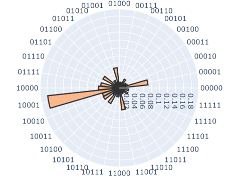
(b) $p/2=0.25$

Figure 8: Probability distribution for the case of two parties with inputs $10$ and $7$, respectively, with identical dephasing noise applied on each entangled qubit pair for varying noise levels, $p/2$, as indicated. The correct outcome is given by $10001$ in binary.

3.2 Depolarising noise

We similarly performed the analysis for depolarising noise instead of dephasing noise. Interestingly, the same probability distributions were found as for dephasing noise, with the same symmetry patterns emerging. We therefore omitted the figures, as they give no additional information compared to the figures in the previous circuit. In the next section, we proof that indeed the probability distributions follow a specific pattern with symmetries, independent of the type of noise.

4 Analytical study

The probability distributions shown in the previous sections showed some symmetry: Some quantum states appear to have the same probabilities. In this section we analytically analyse this symmetry effect and show that, for fixed error probability, indeed the weighted Hamming distance with the correct output string determines the probability of being measured. We first derive an expression for the probability distribution that applies to both dephasing and depolarising noise, and then discuss the intuition on the relation between the analytical expression and the observed pattern.

4.1 Proof of probability distribution

The probability distribution of the distributed quantum summation protocol under dephasing or depolarising noise follows a specific probability distribution.

Lemma 1.

The shared GHZ state under depolarising or dephasing noise for $n$ parties can be written as

$$\rho=\bigotimes_{s=0}^{n-1}\frac{1}{2}(\ket{0}\bra{0}+\ket{1}\bra{1}+\tilde{a_{i}}\ket{0}\bra{1}+\tilde{a_{i}}\ket{1}\bra{0}),$$ (4)

where $\tilde{a_{i}}=(1-p_{i})$ for dephasing noise and $\tilde{a}=1-2p_{i}$ for depolarizing noise, with $p_{i}$ the noise parameter for party $i$.

Proof.

We have $\rho=\frac{1}{2}(\ket{0}^{\otimes n}+\ket{1}^{\otimes n})(\bra{0}^{\otimes n}+\bra{1}^{\otimes n})$. Applying a dephasing noise on qubit $i$ gives

$$\rho \mapsto\Big{(}1-\frac{p_{i}}{2}\Big{)}\rho+\frac{p_{i}}{2}Z_{i}\rho Z_{i}$$

$$=\frac{1}{2}\bigg{(}\ket{0}^{\otimes n}\bra{0}^{\otimes n}+\ket{1}^{\otimes n}\bra{1}^{\otimes n}+(1-p_{i})\Big{(}\ket{0}^{\otimes n}\bra{1}^{\otimes n}+\ket{1}^{\otimes n}\bra{0}^{\otimes n}\Big{)}\bigg{)}.$$

Hence, applying dephasing noise on every qubit, gives

$$\rho\mapsto\frac{1}{2}\prod_{i=0}^{n-1}\bigg{(}\ket{0}^{\otimes n}\bra{0}^{\otimes n}+\ket{1}^{\otimes n}\bra{1}^{\otimes n}+(1-p_{i})\Big{(}\ket{0}^{\otimes n}\bra{1}^{\otimes n}+\ket{1}^{\otimes n}\bra{0}^{\otimes n}\Big{)}\bigg{)}.$$

For depolarising noise, the same expression holds by replacing $p_{i}$ by $2p_{i}$. ∎

Now define $\tilde{a}_{S}=\prod_{S\subseteq\{0,\dots,n-1\}}\tilde{a}_{i}$ and note that with more qubits contributing off-diagonal terms, the total product decreases. As we consider the same error rates for every qubit, we define the fidelity parameter $\tilde{a}$ as $\tilde{a}=\prod_{i=0}^{n-1}\tilde{a}_{i}$. In particular, $\tilde{a}=1$ corresponds to a noiseless GHZ-state, whereas $\tilde{a}=0$ corresponds to a completely dephased or depolarised GHZ state.

Theorem 2.

Let $\{t^{(i)}\}_{i=1}^{m}$ be the inputs of the different parties and let

$$\theta_{s}=\frac{\pi}{2^{n-1-s}}\sum_{i=1}^{m}t^{(i)}=\frac{2\pi}{2^{n-s}}\sum_{i=1}^{m}t^{(i)}.$$ (5)

Then, the $m$-player distributed adder protocol produces the output probability distribution

$$P(x)=\frac{1}{2^{n}}\underset{s=0}{\overset{n-1}{\Pi}}[1+a\cos{(\theta_{s}-2\pi x/2^{n-s})}],$$ (6)

with fidelity parameter $a\in[0,1]$ related to the depolarising or dephasing noise level in the shared GHZ states.

Proof.

The state just before the final inverse quantum Fourier transform is given by

$$\ket{\Psi}=\bigotimes_{s=0}^{n-1}\frac{1}{\sqrt{2}}(\ket{0}+e^{i\theta_{s}}\ket{1})=\bigotimes_{s=0}^{n-1}\frac{1}{\sqrt{2}}\left(\sum_{j_{s}=0,1}e^{i\theta_{s}j_{s}}\ket{j_{s}}\right),$$ (7)

which simplifies to

$$\ket{\Psi}=\frac{1}{\sqrt{2^{n}}}\sum_{j_{=}0}^{2^{n}-1}e^{i\sum_{s=0}^{n-1}\theta_{s}j_{s}}\ket{j_{n-1}\ldots j_{0}}.$$ (8)

From Lemma 1, the presence of dephasing or depolarising noise on the quantum edges mixes the state of the server, such that the density matrix takes the form

$$\rho_{s}=\bigotimes_{s=0}^{n-1}\frac{1}{2}(\ket{0}\bra{0}+\ket{1}\bra{1}+ae^{-i\theta_{s}}\ket{0}\bra{1}+ae^{i\theta_{s}}\ket{1}\bra{0})$$ (9)

which can be written as

$$\rho_{0}=\frac{1}{2^{n}}\sum_{j=0}^{2^{n}-1}\sum_{k=0}^{2^{n}-1}a^{\sum_{s}|k_{s}-j_{s}|}e^{i\sum_{s}(\theta_{s}j_{s}-\theta_{s}k_{s})}\ket{j_{n-1}\ldots j_{0}}\bra{k_{n-1}\ldots k_{0}},$$ (10)

where $a=\tilde{a}^{2}$, as the distributed CNOT gates are performed twice, both before and after the rotations.

The last step of the protocol consists of applying the inverse quantum Fourier transform. It maps the state in Equation (10) to

$$\mathbf{IQFT}_{n}\rho_{0}\mathbf{QFT}_{n}$$

$$\quad=\frac{1}{2^{n}}\sum_{j,k=0}^{2^{n}-1}a^{\sum_{s}|k_{s}-j_{s}|}e^{i\sum_{s}(\theta_{s}j_{s}-\theta_{s}k_{s})}\left(\mathbf{IQFT}_{n}\ket{j_{n-1}\ldots j_{0}}\right)\left(\mathbf{IQFT}_{n}\ket{k_{n-1}\ldots k_{0}}\right)^{\dagger}$$

$$\quad=\frac{1}{2^{2n}}\sum_{x,y=0}^{2^{n}-1}\sum_{j,k=0}^{2^{n}-1}a^{\sum_{s}|k_{s}-j_{s}|}e^{i\sum_{s}\left(\theta_{s}-\frac{\pi}{2^{s}}x\right)j_{s}}e^{-i\sum_{s}\left(\theta_{s}-\frac{\pi}{2^{s}}y\right)k_{s}}\ket{x_{n-1}\ldots x_{0}}\bra{y_{n-1}\ldots y_{0}}.$$ (11)

As the probability of measuring a computational basis state corresponds to the corresponding diagonal element of the density matrix, we obtain the probability $P(x)$ by setting $x=y$:

$$P(x) =\frac{1}{2^{2n}}\sum_{j,k=0}^{2^{n}-1}a^{\sum_{s}|k_{s}-j_{s}|}e^{i\sum_{s}\left(\theta_{s}-\frac{2\pi}{2^{n-s}}x\right)j_{s}}e^{-i\sum_{s}\left(\theta_{s}-\frac{2\pi}{2^{n-s}}x\right)k_{s}}$$

$$=\frac{1}{2^{2n}}\Pi_{s=0}^{n-1}\sum_{j_{s},k_{s}=0,1}a^{|k_{s}-j_{s}|}e^{i\left(\theta_{s}-\frac{2\pi}{2^{n-s}}x\right)j_{s}}e^{-i\left(\theta_{s}-\frac{2\pi}{2^{n-s}}x\right)k_{s}}$$

$$=\frac{1}{2^{2n}}\Pi_{s=0}^{n-1}\left(1+ae^{i\left(\theta_{s}-\frac{2\pi}{2^{n-s}}x\right)}+ae^{-i\left(\theta_{s}-\frac{2\pi}{2^{n-s}}x\right)}+1\right)$$

$$=\frac{1}{2^{n}}\Pi_{s=0}^{n-1}\left[1+a\cos{\left(\theta_{s}-\frac{2\pi}{2^{n-s}}x\right)}\right],$$ (12)

which completes the proof. ∎

4.2 Understanding the noisy distribution

This section provides intuition for what the proven theoretical distribution in Equation (6) actually looks like and how it translates to the distribution observed in the simulations. From the equation, it follows that the probability is maximised for outcomes for which each of the cosines has an argument equal to $2k\pi$ for some integer $k$, given that $a$ is non-negative. Setting $x=\tilde{x}$, with $\tilde{x}$ the correct outcome of the summation, indeed maximises the probability. The resulting probability then equals

$$P(\tilde{x})=\left(\frac{1+a}{2}\right)^{n}.$$

Note that for a noiseless setting where $a=1$, this indeed yields a probability of 1.

Now, if $y\in\mathbb{Z}_{2^{n}}$ is a different outcome, $y$ can be written as $y=\tilde{x}\oplus z$ for some error $z\in\mathbb{Z}_{2^{n}}\backslash\{0\}$. The probability to observe $y$ then equals

$$P(y)=\frac{1}{2^{n}}\prod_{s=0}^{n-1}[1+a\cos(2\pi z/2^{n-s})]$$

Note that each of the factors has a periodic behaviour depending on $z$. Altogether, the periodic factor lead to a periodic behaviour in the probability distribution of the possible outcomes, depending on the Hamming distance between the correct outcome $\tilde{x}$ and the measured outcome $y$.

5 Protocol modifications

One caveat of the DISTRIBUTED-QFT-ADDER protocol is the need for a trusted third party to act as the server. Although this is a common assumption in some classical multi-party computation protocols, it is unrealistic in practice. This section therefore introduces a modification to the protocol which eliminates the necessity of a reliable authority.

First, Threshold Shamir’s Secret Sharing is briefly explained, as it will be the main ingredient of the new protocol. Second, we discuss the protocol modifications.

5.1 Threshold Shamir’s Secret Sharing

Threshold Shamir’s Secret Sharing (SSS) is a well-known classical protocol originally intended to distribute secrets between several entities, with the ability to reconstruct them later [25].

Suppose an agent desires to distribute a secret $X$ among $k$ parties. Then the agent would choose a polynomial of order $t<k$ over a finite field $GF(q)$

$$g(x)=X+a_{1}x+\ldots+a_{t-1}x^{t-1}$$ (13)

with a prime number $q$ such that $X<q$. Next, the secret sharer would choose a set of $k$ different points $\{x_{1},\ldots,x_{k}\}$ to evaluate the polynomial on and would send one polynomial evaluation $g(x_{j})$ to each party. Finally, any subset of $t$ parties can reconstruct the secret by simply performing interpolation with the polynomial evaluations that they received and then determining $g(0)=X$. Importantly, the knowledge of $t-1$ shares $\{(x_{i},g(x_{i}))\}$ does not provide any information about the secret.

5.2 Protocol modification

A key observation is that SSS can be utilized to perform multiparty summation in a secure manner by combining it with repeated usage of DISTRIBUTED-QFT-ADDER. This results in the following protocol:

NO-TP-ADDER

Consider $m$ parties, each holding a number $X_{i}$.

• Step 1: the parties jointly agree on a sufficiently large prime $q$ and make $q$ public;

• Step 2: each party chooses a polynomial of order $t$ over the finite field $GF(q)$

  $$g_{i}(x)=X_{i}+a_{1}^{i}x+\ldots+a_{t-1}^{i}x^{t-1}$$ (14)

  where the coefficients are chosen at random, except for $a_{0}^{i}$ which corresponds to the real input from the party and $a^{i}_{t-1}\neq 0$;

• Step 3: In each round, a different party will act as a server, which requires some order for the parties to act as server: $\sigma\in\mathcal{F}=\{\text{permutations of n elements}\}$;

• Step 4: $m$ rounds of DISTRIBUTED-QFT-ADDER are performed. For each round $r\in\{1,\ldots,m\}$:

  • Party $\sigma(r)$ acts as server;

  • Party $j$ inputs $g_{j}(r)$;

  • Party $\sigma(r)$ computes result of the intermediate summation $s_{r}$ and stores it.

• Step 5: $t$ parties share the intermediate results they stored, which are then used to perform interpolation in order to calculate the polynomial resulting from summing all parties’ polynomials $G(x)=\sum_{i=1}^{m}g_{i}(x)$. The result of the summation can then be obtained evaluating $G(0)=\sum_{i=1}^{m}X_{i}$.

The advantage of this approach is that by having each party act as a server on one round, there is no agent that holds more power or knowledge than any other. Thus, the necessity for a trusted third party is removed, making the protocol more suitable for real life situations.

It is important to note that since the parties only know the intermediate shares $s_{r}$, they cannot reconstruct the secret on their own. Knowledge of at least $t$ shares is needed to recover the result of the summation.

6 Conclusions and outlook

In this work, we investigated the performance of a practical implementation of the multiparty quantum summation protocol [15]. First, we considered that a server party and shared entangled states that undergo depolarizing or dephasing noise. The resulting probability distributions show a clear symmetry, which the analytical study later proved. The magnitude of probability on the erroneous states depends on the amount of noise affecting the execution of the protocol. Knowledge about the distribution of outcomes and the state of the qubits at the end of the protocol could be leveraged in order to increase the probability of successfully retrieving the correct result of the summation.

The existence of a trusted third party is usually not a realistic assumption; thus, building upon the classical Shamir’s Secret Sharing protocol, we presented a modification of DISTRIBUTED-QFT-ADDER to remove the need for a trusted server party. This approach does however increase the number of protocol runs required.

Future work should address the effects of other sources of noise that are present in the protocol, such as imperfect local operations. More importantly, a proper study of the effects that noise has on the security of the protocol needs to be done. As a first step, formal definitions of security, anonymity and privacy in the context of quantum multiparty summation must be established, similar to the contribution that Arapinis et al. had in the field of Quantum Electronic Voting [26].

References

- Shor [1994] P. W. Shor. Algorithms for quantum computation: discrete logarithms and factoring. In Proceedings 35th Annual Symposium on Foundations of Computer Science, page 124–134. IEEE Comput. Soc. Press, 1994. ISBN 978-0-8186-6580-6. doi: 10.1109/SFCS.1994.365700. URL http://ieeexplore.ieee.org/document/365700/.
- Shor [1997] P. W. Shor. Polynomial-Time Algorithms for Prime Factorization and Discrete Logarithms on a Quantum Computer. SIAM J. Comput., 26(5):1484–1509, 1997. doi: 10.1137/S0097539795293172. URL https://doi.org/10.1137/S0097539795293172.
- Fedorov and Gelfand [2021] A. K. Fedorov and M. S. Gelfand. Towards practical applications in quantum computational biology. Nature Computational Science, 1(2):114–119, February 2021. doi: 10.1038/s43588-021-00024-z. URL https://doi.org/10.1038/s43588-021-00024-z.
- Harrow et al. [2009] Aram W. Harrow, Avinatan Hassidim, and Seth Lloyd. Quantum algorithm for linear systems of equations. Phys. Rev. Lett., 103:150502, Oct 2009. doi: 10.1103/PhysRevLett.103.150502. URL https://link.aps.org/doi/10.1103/PhysRevLett.103.150502.
- Eisert et al. [2000] J. Eisert, K. Jacobs, P. Papadopoulos, and M. B. Plenio. Optimal local implementation of nonlocal quantum gates. Phys. Rev. A, 62:052317, Oct 2000. doi: 10.1103/PhysRevA.62.052317. URL https://link.aps.org/doi/10.1103/PhysRevA.62.052317.
- Yimsiriwattana and Lomonaco [2004] Anocha Yimsiriwattana and Samuel J. Lomonaco. Generalized ghz states and distributed quantum computing, 2004. URL https://arxiv.org/abs/quant-ph/0402148.
- Yimsiriwattana and Jr. [2004] Anocha Yimsiriwattana and Samuel J. Lomonaco Jr. Distributed quantum computing: a distributed Shor algorithm. In Eric Donkor, Andrew R. Pirich, and Howard E. Brandt, editors, Quantum Information and Computation II, volume 5436, pages 360 – 372. International Society for Optics and Photonics, SPIE, 2004. doi: 10.1117/12.546504. URL https://doi.org/10.1117/12.546504.
- Beals et al. [2013] Robert Beals, Stephen Brierley, Oliver Gray, Aram W. Harrow, Samuel Kutin, Noah Linden, Dan Shepherd, and Mark Stather. Efficient distributed quantum computing. Proceedings of the Royal Society A: Mathematical, Physical and Engineering Sciences, 469(2153):20120686, May 2013. doi: 10.1098/rspa.2012.0686. URL https://doi.org/10.1098/rspa.2012.0686.
- DiAdamo et al. [2021] Stephen DiAdamo, Marco Ghibaudi, and James Cruise. Distributed quantum computing and network control for accelerated vqe. IEEE Transactions on Quantum Engineering, 2:1–21, 2021. doi: 10.1109/TQE.2021.3057908.
- Gyongyosi and Imre [2021] Laszlo Gyongyosi and Sandor Imre. Scalable distributed gate-model quantum computers. Scientific Reports, 11(1), February 2021. doi: 10.1038/s41598-020-76728-5. URL https://doi.org/10.1038/s41598-020-76728-5.
- Caleffi et al. [2022] Marcello Caleffi, Michele Amoretti, Davide Ferrari, Daniele Cuomo, Jessica Illiano, Antonio Manzalini, and Angela Sara Cacciapuoti. Distributed quantum computing: a survey, 2022.
- Neumann et al. [2020] Niels MP Neumann, Roy van Houte, and Thomas Attema. Imperfect distributed quantum phase estimation. In Computational Science–ICCS 2020: 20th International Conference, Amsterdam, The Netherlands, June 3–5, 2020, Proceedings, Part VI 20, pages 605–615. Springer, 2020.
- Khabiboulline et al. [2021] Emil T. Khabiboulline, Juspreet Singh Sandhu, Marco Ugo Gambetta, Mikhail D. Lukin, and Johannes Borregaard. Efficient quantum voting with information-theoretic security, 2021. URL https://arxiv.org/abs/2112.14242.
- Barenco et al. [1995] Adriano Barenco, Charles H. Bennett, Richard Cleve, David P. DiVincenzo, Norman Margolus, Peter Shor, Tycho Sleator, John A. Smolin, and Harald Weinfurter. Elementary gates for quantum computation. Phys. Rev. A, 52:3457–3467, 11 1995. doi: 10.1103/PhysRevA.52.3457. URL https://link.aps.org/doi/10.1103/PhysRevA.52.3457.
- Neumann and Wezeman [2022] Niels M. P. Neumann and Robert S. Wezeman. Distributed quantum machine learning. In Frank Phillipson, Gerald Eichler, Christian Erfurth, and Günter Fahrnberger, editors, Innovations for Community Services, pages 281–293, Cham, 2022. Springer International Publishing. ISBN 978-3-031-06668-9.
- Draper [2000] Thomas G. Draper. Addition on a quantum computer, 2000. URL https://arxiv.org/abs/quant-ph/0008033.
- Ruiz-Perez [2017] J.C. Ruiz-Perez, L.; Garcia-Escartin. Quantum arithmetic with the quantum fourier transform. Quantum Information Processing, 2017. doi: https://doi.org/10.1007/s11128-017-1603-1. URL https://link.springer.com/article/10.1007/s11128-017-1603-1.
- Hermans et al. [2022] S. L. N. Hermans, M. Pompili, H. K. C. Beukers, S. Baier, J. Borregaard, and R. Hanson. Qubit teleportation between non-neighbouring nodes in a quantum network. Nature, 605(7911):663–668, may 2022. doi: 10.1038/s41586-022-04697-y. URL https://doi.org/10.1038%2Fs41586-022-04697-y.
- Li et al. [2023] Zhiyuan Li, Pei Liu, Peng Zhao, Zhenyu Mi, Huikai Xu, Xuehui Liang, Tang Su, Weijie Sun, Guangming Xue, Jing-Ning Zhang, et al. Error per single-qubit gate below in a superconducting qubit. npj Quantum Information, 2023. doi: 10.1038/s41534-023-00781-x.
- Wu et al. [2013] Qing-Lin Wu, Naoto Namekata, and Shuichiro Inoue. High-fidelity entanglement swapping at telecommunication wavelengths. Journal of Physics B: Atomic, Molecular and Optical Physics, 46(23):235503, nov 2013. doi: 10.1088/0953-4075/46/23/235503. URL https://dx.doi.org/10.1088/0953-4075/46/23/235503.
- Xu et al. [2016] Jin-Shi Xu, Man-Hong Yung, Xiao-Ye Xu, Jian-Shun Tang, Chuan-Feng Li, and Guang-Can Guo. Robust bidirectional links for photonic quantum networks. Science Advances, 2(1):e1500672, 2016. doi: 10.1126/sciadv.1500672. URL https://www.science.org/doi/abs/10.1126/sciadv.1500672.
- Šafránek et al. [2015] Dominik Šafránek, Mehdi Ahmadi, and Ivette Fuentes. Quantum parameter estimation with imperfect reference frames. New Journal of Physics, 17(3):033012, mar 2015. doi: 10.1088/1367-2630/17/3/033012. URL https://dx.doi.org/10.1088/1367-2630/17/3/033012.
- van Dam [2022] Janice van Dam. Analytical model of satellite based entanglement distribution. Master’s thesis, TU Delft, 2022. URL http://resolver.tudelft.nl/uuid:ad64c61c-99a3-42e8-8451-9758b11261e6.
- tA v et al. [2021] A tA v, MD SAJID ANIS, Abby-Mitchell, Héctor Abraham, AduOffei, and Rochisha Agarwal et al. Qiskit: An open-source framework for quantum computing, 2021.
- Shamir [1979] Adi Shamir. How to share a secret. Commun. ACM, 22(11):612–613, nov 1979. ISSN 0001-0782. doi: 10.1145/359168.359176. URL https://doi.org/10.1145/359168.359176.
- Arapinis et al. [2021] Myrto Arapinis, Nikolaos Lamprou, Elham Kashefi, and Anna Pappa. Definitions and security of quantum electronic voting. ACM Transactions on Quantum Computing, 2(1):1–33, 2021.