Gravitational wave fluxes on generic orbits in Kerr spacetime: higher spin and large eccentricity

Abstract

To obtain the waveform template of gravitational waves (GWs), substantial computational resources and exceedingly high precision are often required. In the previous study [JCAP 11 (2023) 070], we efficiently and accurately calculate GW fluxes of a particle in circular orbits around a Schwarzschild black hole using the confluent Heun function. We extend the previous method to calculate the asymptotic GW fluxes from a particle in generic orbits around a Kerr black hole. Especially when dealing with the computational difficulties in large eccentricity $e=0.9$, higher spin $a=0.999$, higher harmonic modes and strong-field regions, our results are much better than the high-order post-Newtonian results and comparable to the results of the Mano-Suzuki-Takasugi method. Using the grid data of the asymptotic GW fluxes, we give the adiabatic waveform of non-rotating black holes, which agrees well with the waveforms of numerical relativity.

1 Introduction

The two-body problem holds a crucial position in general relativity. It has garnered significant attention in the field of GW astronomy due to the potential of binary black holes (BBHs) inspirals to generate GWs, which are expected to be detected directly by ongoing GW observatories worldwide [1, 2, 3, 4, 5]. Future space-based GW detectors, such as the Laser Interferometer Space Antenna (LISA) [6, 7], TianQin [8, 9], and Taiji [10], will be built with the specific purpose of detecting GW signals from sources that radiate in the millihertz bandwidth, namely extreme mass ratio inspirals (EMRIs). EMRI events enable the precise mapping of black hole (BH) spacetimes, allowing for the accurate determination of BH masses and spins. This offers an opportunity to test the hypothesis that astrophysical BHs conform to Kerr spacetime [11]. To comprehend the dynamics of BBHs, accurately predicting GW waveforms is essential for effectively detecting signals in observed data.

A primary approach to achieve this purpose is calculations of gravitational self-force (GSF) within black hole perturbation (BHP) theory. The system of BBHs is considered as a point mass orbiting a black hole, and its dynamics can be described by the equation of motion that includes the effect of the interaction with its self-field, known as the GSF. The formalism of GSF calculations was initially established by Mino, Sasaki, and Tanaka in the mid-1990s [12], along with Quinn and Wald [13]. Over the past two decades, this formalism has seen significant refinement to improve both its mathematical rigor and conceptual clarity. For comprehensive reviews and further research on the GSF, please refer to Refs. [14, 15, 16, 17, 18].

One commonly employed approach to compute the complete GSF involves utilizing the Weyl scalars $\psi_{0}$ and $\psi_{4}$ that satisfy the separable Teukolsky equation [19, 20, 21, 22]. These scalars contain the majority of the gauge invariant information regarding the complete metric perturbation [23]. In the 1970s, Chrzanowski, Cohen, and Kegeles (CCK) [24, 25, 26] developed a method to reconstruct vacuum metric perturbations in a radiation gauge from vacuum solutions of $\psi_{0}$ and $\psi_{4}$. However, as Ori pointed out [27], when this method is applied to the field generated by a point particle source, the resulting metric perturbation becomes highly singular. The singularities in the metric perturbation are not only found at the position of the particle, but also manifest as a stringlike gauge singularity that extends from the particle to the event horizon or infinity. It is uncertain whether the established GSF form can be extended to account for this type of singularity. Subsequently, Pound et al. [28] discovered that the GSF can be extracted from the metric perturbations in the radiation gauge. Friedman’s group [29, 30, 31] pioneered the radiation gauge method of the GSF, and they calculated the Detweiler redshift invariance on the circular equatorial orbit of the Kerr spacetime [32]. Maarten extended their method to calculate the first-order GSF and redshifts on eccentric equatorial orbits [33, 34] and generic bound orbits[35](featuring both eccentricity and inclination). Furthermore, while $\psi_{0}$ or $\psi_{4}$ carry most of the information regarding metric perturbations, the perturbations of “mass” and “angular momentum” must be recovered through alternative methods [23]. Merlin et al. [36] reconstructed these components for fields sourced by a particle in equatorial orbits by imposing the continuity of certain gauge-invariant fields derived from the metric. The results are characterized by simplicity: Outside the particle’s orbit, the mass and angular momentum perturbations are solely determined by the orbital energy and orbital angular momentum, while both perturbations vanish within the orbit. Using the direct method of metric perturbation generated by the CCK procedure, it is demonstrated that this result is indeed applicable to any compact source in the radial direction [37].

Much progress has been achieved in calculating the complete GSF for various orbits, but it remains particularly challenging for generic orbits, especially in Kerr spacetime. Three fundamental frequencies ${\Omega_{r,\theta,\phi}}$ characterize the generic geodesic orbits. However, calculating these frequencies is considerably difficult, and no efficient and accurate method for the GSF calculations of generic orbits has been developed thus far. Due to the regularization problem of the point mass limit, high-precision GSF requires magnanimous computational cost in practical calculations. Therefore, it is very crucial to study a method to reduce the computational cost of GSF. The two-timescale expansion method [38] provides a hint: assuming that a point mass does not encounter any transient resonance [39], the orbital phase is the most significant information for the prediction of the GW waveform, which can be written as

$$\Phi=\epsilon^{-1}\left[\Phi^{(0)}+\epsilon\Phi^{(1)}+O(\epsilon^{2})\right],$$ (1.1)

where the mass ratio $\epsilon={m_{2}}/{m_{1}}\leq 1$. And the leading-order term $\Phi^{(0)}$ can be considered as the time-averaged dissipative effect of the first-order GSF. The calculation of this secular effect can be simplified by defining the radiative field as half of the retarded solution of the gravitational perturbation equation minus half of the advanced solution, using the adiabatic approximation method [40, 41]. This is effective because the radiative field is a homogeneous solution of the divergence that is induced by the point mass limit. By using this method, the leading-order term can be accurately calculated without huge computational cost. On the other hand, $\Phi^{(1)}$ corresponds to the residual part of the first-order GSF, which includes the the oscillatory part of both the dissipative and conservative GSFs, as well as the time-averaged dissipative part of the second-order GSF. Currently, there is no simplified approach available to calculate these post-adiabatic components accurately. However, since $\Phi^{(1)}$ is considered a minor factor, the requirement for precision is not stringent. This fact suggests that the computational burden can be reduced by employing suitable methods with appropriate fault tolerance to compute each piece of the GSF. Based on this formalism, Osburn et al. proposed a hybrid scheme for calculating the GSF of eccentric orbits [42].

For non-spinning particles in generic orbits around a Kerr BH, the time-averaged dissipative part of the first-order GSF is the dominant contribution to the inspiral evolution in Kerr spacetime, making it suitable for calculating GW fluxes necessary for constructing GW waveforms. By using the Teukolsky equation to calculate the dissipative first-order GSF, there have been some breakthroughs. Hughes successfully solved the short-range potential form (Sasaki-Nakamura equation) of the Teukolsky equation by numerical integration [44], and provide the inspiral evolution and snapshot waveforms for spherical orbits (circular and nonequatorial) in Kerr spacetime [45]. Based on the frequency-domain orbit function of Kerr BHs [46], his group extended the GSF to generic orbits[47]. After years of research, his group also gave a long inspiral waveform of EMRIs in generic orbits [48]. Moreover, they calculated the EMRI waveforms [49] of a spinning body moving on generic orbits in the second-order spin by using the frequency-domain method proposed in Refs. [50, 51]. Fujita’s group from Japan first used the Mano-Suzuki-Takasugi (MST) method to give an efficient numerical method for calculating the dissipative GSF of generic orbits [52]. Then, based on the MST method and the analytical solution of bound timelike geodesic orbits in Kerr spacetime [53], they derived the analytical formula of high-order post-Newtonian (PN) expansion [54]. They used this analytical formula to study the measurability of EMRI waves by LISA, and their discussion was mainly about the adiabatic waveforms of eccentric and equatorial sources [55]. Their numerical and analytical methods are widely used in the construction of waveforms with any mass ratio [56, 57]. The results of these two teams have excellent computational performance. Their methods can not only calculate the dissipative GSF of generic orbits in Kerr spacetime with large eccentricities, large inclinations, high harmonic modes, and strong-field regions, but also exhibit extremely high computational accuracy. Other EMRI waveforms or GSF calculations can only calculate small eccentricity ($e\leq 0.3$) or Schwarzschild BHs [35, 58, 59]. Our previous study [60] proposed an exact approach to calculate GW fluxes from a particle in circular orbits around a Schwarzschild BH using the confluent Heun function. The computational accuracy and efficiency of this exact approach are comparable to those of the MST method and the numerical integration method.

In this work, we extend the previous work to obtain GW radiative fluxes form a particle in generic orbits around a Kerr BH. We aim to compute and store the grid data of radiative fluxes so that it can cover the extreme cases of orbital parameters: $a=0.999,e=0.9,$ large inclinations and high harmonic modes. This work will provide an accurate and efficient choice of energy flux data and GW amplitudes for waveform construction.

The remainder of the paper is arranged as follows. Section 2 provide a brief review of the geodesic motion of a point particle in Kerr spacetime. In Section 3, we give the exact solution of the Teukolsky equation of the Kerr BH in the form of the confluent Heun function, which is used to calculate the radiative energy fluxes on the generic orbit. Section 4 is devoted to comparing our results with those of PN expansion and the MST methods to validate the high precision of our approach. Finally, the conclusion of this paper is presented in Section 5, which includes plans and directions for future work. In this paper, we use geometrized units: $c=G=1$.

2 Kerr geodesics

In this section, we discuss bounded Kerr geodesics. The detailed content can be seen in Refs.[61, 46, 47, 53, 54, 62, 48], we briefly review the geodesic dynamics of a point particle in the Kerr spacetime. Some lengthy but important formulas are given in Appendix A.

Firstly, the Kerr metric in the Boyer-Lindquist coordinates, $(t,r,\theta,\varphi)$, can be given by

$$g_{\mu\nu}dx^{\mu}dx^{\nu} =-\left(1-\frac{2Mr}{\Sigma}\right)dt^{2}-\frac{4Mar\sin^{2}\theta}{\Sigma}dtd\varphi+\frac{\Sigma}{\Delta}dr^{2}$$

$$+\Sigma d\theta^{2}+\left(r^{2}+a^{2}+\frac{2Ma^{2}r}{\Sigma}\sin^{2}\theta\right)\sin^{2}\theta d\varphi^{2},$$ (2.1)

where $\Sigma=r^{2}+a^{2}\cos^{2}\theta$, $\Delta=({r-{r_{-}}})({r-{r_{+}}})$ and ${r_{\pm}}=M\pm\sqrt{{M^{2}}-{a^{2}}}$. $r_{-}$ is the inner horizon, and $r_{+}$ is the outer (event) horizon. Here, $M$ and $aM$ are the mass and angular momentum of the Kerr BH, respectively.

2.1 Formulations of orbital frequencies

We use Mino time as our time parameter to describe these bound orbits [53, 48]. An interval of Mino time $d\lambda$ is related to an interval of proper time $d\tau$ by $d\lambda=d\tau/\Sigma$, the geodesic equations become

$$\left(\frac{dr}{d\lambda}\right)^{2} =[E(r^{2}+a^{2})-aL_{z}]^{2}-\Delta[r^{2}+(L_{z}-aE)^{2}+Q]\equiv R(r),$$ (2.2)

$$\left(\frac{d\theta}{d\lambda}\right)^{2} =Q-\cot^{2}\theta L_{z}^{2}-a^{2}\cos^{2}\theta(1-E^{2})\equiv\Theta(\theta)\;,$$ (2.3)

$$\frac{d\phi}{d\lambda} =\csc^{2}\theta L_{z}+\frac{2MraE}{\Delta}-\frac{a^{2}L_{z}}{\Delta}\equiv\Phi_{r}(r)+\Phi_{\theta}(\theta)\;,$$ (2.4)

$$\frac{dt}{d\lambda} =E\left[\frac{(r^{2}+a^{2})^{2}}{\Delta}-a^{2}\sin^{2}\theta\right]-\frac{2MraL_{z}}{\Delta}\equiv T_{r}(r)+T_{\theta}(\theta)\;.$$ (2.5)

where $E$, $L_{z}$, and $Q$ are the orbit’s energy (per unit $\mu$), axial angular momentum (per unit $\mu$), and Carter constant (per unit $\mu^{2}$), respectively. The expressions of these quantities are shown in Eq. A.1, A.2 and A.3.

It can be seen from Eqs. 2.2 and 2.3 that the bound orbit of the radial and the polar motion is periodic when parameterized using $\lambda$:

$$r(\lambda)=r(\lambda+n\Lambda_{r})\;,\quad\theta(\lambda)=\theta(\lambda+k\Lambda_{\theta})\;,$$ (2.6)

where $n$ and $k$ are integers. For fundamental periods $\Lambda_{r,\theta,\phi}$, we can define the associated frequencies: $\Upsilon_{r,\theta,\phi}=2\pi/\Lambda_{r,\theta,\phi}$. The orbital motions in $t$ and $\phi$ is the sum of the long-term cumulative part and oscillation functions:

$$t(\lambda) =t_{0}+{\Upsilon_{t}}\lambda+\Delta t_{r}[r(\lambda)]+\Delta t_{\theta}[\theta(\lambda)]\;,$$ (2.7)

$$\phi(\lambda) =\phi_{0}+\Upsilon_{\phi}\lambda+\Delta\phi_{r}[r(\lambda)]+\Delta\phi_{\theta}[\theta(\lambda)]\;.$$ (2.8)

where $t_{0}$ and $\phi_{0}$ describe initial conditions,

$${\Upsilon_{t}}=\langle T_{r}(r)\rangle+\langle T_{\theta}(\theta)\rangle\;,\quad\Upsilon_{\phi}=\langle\Phi_{r}(r)\rangle+\langle\Phi_{\theta}(\theta)\rangle\;,$$ (2.9)

$$\Delta t_{r}[r(\lambda)] =T_{r}[r(\lambda)]-\langle T_{r}(r)\rangle\equiv\Delta t_{r}(\lambda)\;,\quad\Delta t_{\theta}[\theta(\lambda)]=T_{\theta}[\theta(\lambda)]-\langle T_{\theta}(\theta)\rangle\equiv\Delta t_{\theta}(\lambda)\;,$$ (2.10)

$$\Delta\phi_{r}[r(\lambda)] =\Phi_{r}[r(\lambda)]-\langle\Phi_{r}(r)\rangle\equiv\Delta\phi_{r}(\lambda)\;,\quad\Delta\phi_{\theta}[\theta(\lambda)]=\Phi_{\theta}[\theta(\lambda)]-\langle\Phi_{\theta}(\theta)\rangle\equiv\Delta\phi_{\theta}(\lambda)\;.$$ (2.11)

The quantity ${\Upsilon_{t}}$ and $\Upsilon_{\phi}$ are the frequencies of coordinate time $t$ and $\phi$ with respect to $\lambda$ respectively. The averages $\langle{T_{r,\theta}}\rangle$ and $\langle{\Phi_{r,\theta}}\rangle$ in Eq. 2.9, 2.10 and 2.11 are given by

$$\langle{T_{r}}(r)\rangle =\frac{1}{{{\Lambda_{r}}}}\int_{0}^{{\Lambda_{r}}}{{T_{r}}}[r(\lambda)]{\kern 1.0pt}d\lambda\;,\quad\langle{T_{\theta}}(r)\rangle=\frac{1}{{{\Lambda_{\theta}}}}\int_{0}^{{\Lambda_{\theta}}}{{T_{\theta}}}[\theta(\lambda)]{\kern 1.0pt}d\lambda\;,$$ (2.12)

$$\langle{\Phi_{r}}(r)\rangle =\frac{1}{{{\Lambda_{r}}}}\int_{0}^{{\Lambda_{r}}}{{\Phi_{r}}}[r(\lambda)]{\kern 1.0pt}d\lambda\;,\quad\langle{\Phi_{\theta}}(r)\rangle=\frac{1}{{{\Lambda_{\theta}}}}\int_{0}^{{\Lambda_{\theta}}}{{\Phi_{\theta}}}[\theta(\lambda)]{\kern 1.0pt}d\lambda\;.$$ (2.13)

The observer-time frequencies can be written as

$${\Omega_{r,\theta,\phi}}=\frac{{{\Upsilon_{r,\theta,\phi}}}}{{\Upsilon_{t}}}.$$ (2.14)

2.2 Orbit parameterization and initial conditions

The orbit ranges of radial and polar motion are set to $\theta_{\rm min}\leq\theta\leq\theta_{\rm max}$ and $r_{\rm min}\leq r\leq r_{\rm max}$, respectively. Here, $\theta_{\rm max}=\pi-\theta_{\rm min}$ and $r_{\rm min/max}={p}/({1\pm e})$. In order to avoid ambiguity, we use the inclination angle $I$ instead of $\theta_{\rm min}$, and their relation is $I=\pi/2-\mbox{sgn}(L_{z})\theta_{\rm min}$. Because it can smoothly change from $0$ for equatorial prograde to $\pi$ for equatorial retrograde. The cosine of the inclination angle, $x_{I}\equiv\cos I$, is an excellent parameter to describe inclination: $x_{I}$ varies smoothly from $1$ to $-1$ as orbits vary from prograde equatorial to retrograde equatorial, with $L_{z}$ having the same sign as $x_{I}$. The generic geodesic orbit in Kerr spacetime can be characterized by three parameters, $(E,L_{z},Q)$. However, for the bound orbit, another set of parameters $(p,e,x_{I})$ is chosen for convenience [61, 62].

Eqs. 2.7 and 2.8 can give the initial conditions $t_{0}$ and $\phi_{0}$. To set initial conditions in the $r$ and $\theta$ directions, we introduce anomaly angles $\chi_{r}$ and $\chi_{\theta}$ to reparameterize these coordinate motions.

$$r = \frac{p}{1+e\cos(\chi_{r}+\chi_{r0})}\;,$$ (2.15)

$$\cos\theta = \sqrt{1-x_{I}^{2}}\cos(\chi_{\theta}+\chi_{\theta 0})\;.$$ (2.16)

We set $\chi_{\theta}=0$, $\chi_{r}=0$, $t=t_{0}$, and $\phi=\phi_{0}$ when $\lambda=0$. The phase $\chi_{r0}$ then determines $r(0)$, and $\chi_{\theta 0}$ determines the corresponding value of $\theta$. When $\chi_{\theta 0}=0$, the orbit has $\theta=\theta_{\rm min}$ when $\lambda=0$; when $\chi_{r0}=0$, it has $r=r_{\rm min}$ when $\lambda=0$.

We define fiducial geodesic as the geodesic that has $\chi_{\theta 0}=\chi_{r0}=\phi_{0}=0=t_{0}$. The quantity with a “check-mark” indicates that the quantity is along the fiducial geodesic. Such as $\check{r}(\lambda)$ and $\check{\theta}(\lambda)$ are radial and polar directions along the fiducial geodesic.

For non-fiducial geodesics, we introduce definitions: when $r=r_{\rm min}$, $\lambda_{r0}=\min(\lambda)$; when $\theta=\theta_{\rm min}$, $\lambda_{\theta 0}=\min(\lambda)$. This means that

$$r(\lambda)=\check{r}(\lambda-\lambda_{r0})\;,\quad\theta(\lambda)=\check{\theta}(\lambda-\lambda_{\theta 0})\;,$$ (2.17)

These definitions show that these motions are periodic: $r(\lambda_{r0}+n\Lambda_{r})=r_{\rm min}$ for any integer $n$, and $\theta(\lambda_{\theta 0}+k\Lambda_{\theta})=\theta_{\rm min}$ for any integer $k$. There is the relations between $\lambda_{\theta 0}$ and $\chi_{\theta 0}$, and between $\lambda_{r0}$ and $\chi_{r0}$. A useful corollary is

$$\Delta t_{r}(\lambda) = \Delta\check{t}_{r}(\lambda-\lambda_{r0})-\Delta\check{t}_{r}(-\lambda_{r0})\;,$$

$$\Delta t_{\theta}(\lambda) = \Delta\check{t}_{\theta}(\lambda-\lambda_{\theta 0})-\Delta\check{t}_{\theta}(-\lambda_{\theta 0})\;,$$ (2.18)

with analogous formulas for $\Delta\phi_{r}$ and $\Delta\phi_{\theta}$.

Many of the definitions in this section are derived from Hughes’ latest review of bound Kerr geodesics [48]. The introduction of these quantities $(\chi_{r0},\chi_{\theta 0},\phi_{0})$ facilitates the calculation of inspiral evolution in the adiabatic approximation.

3 GW Radiative Fluxes via the Teukolsky equation

The next key in constructing adiabatic inspirals is the calculation of the dissipative part of the first-order GSF. It can give the associated gravitational wave amplitude and radiative fluxes. In this section, we extend the previous method [60] to the Kerr spacetime to calculate these quantities.

3.1 Excat Solutions of Teukolsky equations

In the Teukolsky formalism, the gravitational perturbation of a Kerr black hole is described in terms of the null-tetrad component of the Weyl tensors $\psi_{0}$ and $\psi_{4}$, which satisfy the master equation [20]. The Weyl scalar $\Psi_{4}$ is related to the GW amplitude at infinity as

$$\psi_{4}\rightarrow\frac{1}{2}(\ddot{h}_{+}-i\,\ddot{h}_{\times}),\,\,\,{\rm for}\,\,\,r\rightarrow\infty.$$ (3.1)

The master equation for $\psi_{4}$can be separated into radial and angular parts if we expand $\psi_{4}$ in Fourier harmonic modes as

$$\rho^{-4}\psi_{4}=\displaystyle\sum_{\ell m}\int_{-\infty}^{\infty}d\omega e^{-i\omega t+im\varphi}\ _{-2}S_{\ell m}^{a\omega}(\vartheta)R_{\ell m\omega}(r),$$ (3.2)

where $\rho=(r-ia\cos\vartheta)^{-1}$, and the angular function ${}_{-2}S_{\ell m}^{a\omega}(\vartheta)$ is the spin-weighted spheroidal harmonic with spin $s=-2$. The radial function $R_{\ell m\omega}(r)$ satisfies the radial Teukolsky equation,

$$\left[{\Delta^{-s+1}\frac{d}{{dr}}\Delta^{s+1}\frac{d}{{dr}}+V(r)}\right]{R_{\ell m\omega}}={\Delta}{T_{\ell m\omega}},$$ (3.3)

and the potential term $V(r)$ is given as

$$V(r)={K^{2}}-isK\Delta^{\prime}+\Delta\left({2isK^{\prime}-\hat{\lambda}}\right),$$ (3.4)

where $K=(r^{2}+a^{2})\omega-ma$ and $\hat{\lambda}$ is the eigenvalue of ${}_{-2}S_{\ell m}^{a\omega}(\vartheta)$. The computational methods of the angular function ${}_{-2}S_{\ell m}^{a\omega}(\vartheta)$ and the source function ${T_{\ell m\omega}}$ are discussed in Refs. [44, 63, 64].

The most commonly used methods for solving the homogenous solutions $R^{\rm in,up}_{\ell m\omega}$ of the Teukolsky equation are the PN expansion [65, 66, 67, 68] of the Sasaki-Nakamura equation and the MST method [63, 69, 70]. We presented a excat approach that surpasses the MST method in terms of accuracy for calculating gravitational radiation at the horizon and infinity. The key pieces of our approach have been summarized in depth in the previous paper [60]. Here, we provide a very brief sketch largely to set the context for the following discussion. The general solution of the homogenous form of Eq. 3.3 is derived by the linear combination of two linearly independent particular solutions.

$${R_{\ell m\omega}}={C_{1}}S_{0}^{\beta}(x){\rm{HeunC}}(\alpha,\beta,\gamma,\delta,\eta;x)+{C_{2}}S_{0}^{-\beta}(x){\rm{HeunC}}(\alpha,-\beta,\gamma,\delta,\eta;x),$$ (3.5)

where $C_{1}$ and $C_{2}$ are constants that should be determined based on different boundary conditions. Here, ${\rm{HeunC}}$ is the confluent Heun function [71, 72, 73], and $x$ is defined as a new coordinate that is obtained by applying a Möbius (isomorphic) transformation, which is a linear fractional transformation of the form

$$x=-\frac{{r-r_{+}}}{{r_{+}}-{r_{-}}},$$ (3.6)

and the unnormalized S-homotopic transformation,

$$S_{\rm{0}}^{\beta}(x)={\left({-x}\right)^{\frac{1}{2}(\beta-s)}}{\left({1-x}\right)^{\frac{1}{2}(\gamma-s)}}{{\rm{e}}^{\frac{1}{2}\alpha x}},$$ (3.7)

and the parameters $\alpha$, $\beta$, $\gamma$, $\delta$, and $\eta$ are given by

$$\alpha =-2i\omega{r_{\rm{x}}},$$ (3.8a)

$$\beta =-s+{r_{\rm{x}}}^{-1}\left({2i\omega(r_{+}^{2}+{a^{2}})-2iam}\right),$$ (3.8b)

$$\gamma =s+{r_{\rm{x}}}^{-1}\left({2i\omega(r_{-}^{2}+{a^{2}})-2iam}\right),$$ (3.8c)

$$\delta =2\omega{r_{\rm{x}}}(\omega({r_{-}}+{r_{+}})+is),$$ (3.8d)

$$\eta =2is\omega{r_{+}}-\frac{1}{2}{s^{2}}-s-\hat{\lambda}-2r_{\rm{x}}^{-2}(\omega{r_{\rm{m}}}-am)(\omega{\hat{r}_{\rm{o}}}-am).$$ (3.8e)

where ${r_{\rm{x}}}={r_{-}}-{r_{+}},\hat{r}_{\rm o}={a^{2}}+2{r_{-}}{r_{+}}-r_{+}^{2}$, and $r_{\rm m}=r_{+}^{2}+{a^{2}}$. A more detailed derivation of the general solution (3.5) of the homogeneous Teukolsky equation can be seen in our previous work[60]. However, this derivation did not include the ingoing wave and outgoing wave solution for the Kerr spacetime, and their asymptotic amplitudes. Next, we will present the analytical expressions for these solutions.

The selection of the general solution (3.5) is advantageous in constructing the solutions that satisfy the normalized boundary conditions of the pure ingoing wave $R^{\rm in}_{\ell\omega}(r)$ at the horizon and the pure outgoing wave $R^{\rm up}_{\ell\omega}(r)$ at infinity. Such as

$$R_{\ell m\omega}^{{\rm{in}}}\to\left\{{\begin{array}[]{*{20}{l}}{{\Delta^{-s}}{{\rm{e}}^{-iP{r^{*}}}},}&{r\to r_{\rm H}},\\ {{{B_{\ell m\omega}^{{\rm{ref}}}}}{r^{1-2s}}{{\rm{e}}^{i\omega{r^{*}}}}+{{B_{\ell m\omega}^{{\rm{inc}}}}}{r^{-1}}{{\rm{e}}^{-i\omega{r^{*}}}},}&{r\to+\infty,}\end{array}}\right.$$ (3.11)

$$R_{\ell m\omega}^{{\rm{up}}}\to\left\{{\begin{array}[]{*{20}{l}}{C_{\ell m\omega}^{{\rm{up}}}{{\rm{e}}^{iP{r^{*}}}}+{C_{\ell m\omega}^{{\rm{ref}}}}{\Delta^{-s}}{{\rm{e}}^{-iP{r^{*}}}},}&{r\to{r_{\rm H}},}\\ {{r^{1-2s}}{{\rm{e}}^{i\omega{r^{*}}}},}&{r\to+\infty,}\end{array}}\right.$$ (3.14)

where ${P}=\omega-m\Omega_{\rm H}$ and $\Omega_{\rm H}=\frac{a}{2Mr_{+}}$. Here, $r^{*}$ is the tortoise coordinate defined by

$${r^{*}}=r+\frac{{2M{r_{+}}}}{{{r_{+}}-{r_{-}}}}\ln\frac{{r-{r_{+}}}}{{2M}}-\frac{{2M{r_{-}}}}{{{r_{+}}-{r_{-}}}}\ln\frac{{r-{r_{-}}}}{{2M}}.$$ (3.15)

To construct two solutions $R_{\ell m\omega}^{{\rm{in,up}}}$ satisfying the boundary conditions, only the coefficients $C_{1}$ and $C_{2}$ in the general solution (3.5) are required. Prior to undertaking this task, it becomes imperative to determine the asymptotic expressions of the confluent Heun function in the vicinity of the horizon and at infinity, respectively.

Expanding the confluent Heun function in a sector around the irregular singular point at event horizon $x=0$ and infinity $x=\infty$, the asymptotic behavior at infinity can be expressed as:

$$\mathop{\lim}\limits_{x\to 0}{\rm{HeunC}}(\alpha,\beta,\gamma,\delta,\eta;x)=1,$$ (3.16a)

$$\mathop{\lim}\limits_{\left|x\right|\to\infty}{\rm{HeunC}}(\alpha,\beta,\gamma,\delta,\eta;x)\to D_{\odot}^{\beta}\;{x^{-\frac{{\beta+\gamma+2}}{2}-\frac{\delta}{\alpha}}}+D_{\otimes}^{\beta}{{\rm{e}}^{-\alpha x}}{x^{-\frac{{\beta+\gamma+2}}{2}+\frac{\delta}{\alpha}}},$$ (3.16b)

where ${{D}_{\otimes}^{\beta}}$ and ${{D}_{\odot}^{\beta}}$ are constants, and their analytical expressions is shown in Appendix B.

Using the asymptotic properties (3.16) of the confluent Heun function and the boundary conditions (3.11) of the ingoing wave, we can construct the ingoing wave solution. The ingoing wave solution at the horizon has purely ingoing property, which imply $C_{2}^{\rm in}=0$. Thus, the ingoing wave solution $R_{\ell m\omega}^{{\rm{in}}}$ is given by

$$R_{\ell m\omega}^{{\rm{in}}}=S_{0}^{\beta}(x){\rm{HeunC}}(\alpha,\beta,\gamma,\delta,\eta;x).$$ (3.17)

By utilizing the asymptotic behavior (3.11) of the solution $R_{\ell m\omega}^{{\rm{in}}}$ as $r\rightarrow\infty$, we derive analytic expressions for the asymptotic amplitudes $B_{\ell m\omega}^{\rm inc}$ and $B_{\ell m\omega}^{\rm ref}$,

$$B_{\ell m\omega}^{{\rm{inc}}}={(-{r_{\rm{x}}})^{1-2s+i\frac{{ma}}{{{r_{+}}}}}}{\left({2M}\right)^{-i\frac{{ma}}{{{r_{+}}}}}}{{\rm{e}}^{i\frac{{ma}}{{2M}}}}{(-1)^{-\frac{{\beta+\gamma+2}}{2}-\frac{\delta}{\alpha}}}\;D_{\odot}^{\beta},$$ (3.18a)

$$B_{\ell m\omega}^{{\rm{ref}}}=(-{r_{\rm{x}}}){\left({-\frac{{2M}}{{{r_{\rm{x}}}}}}\right)^{2iM(P+\omega)}}{{\rm{e}}^{-i(P+\omega){r_{+}}}}{(-1)^{-\frac{{\beta+\gamma+2}}{2}+\frac{\delta}{\alpha}}}D_{\otimes}^{\beta}.$$ (3.18b)

Similarly, according to the asymptotic properties (3.16) of the HeunC function and the boundary conditions (3.14) of the outgoing wave, we can construct the outgoing wave solution, can be given by

$$R_{\ell m\omega}^{{\rm{up}}}=\Big{[}{\left({-1}\right)^{\beta+1}}{\frac{{D_{\odot}^{-\beta}}}{{D_{\odot}^{\beta}}}}S_{0}^{\beta}(x){\rm{HeunC}}(\alpha,\beta,\gamma,\delta,\eta;x)+S_{0}^{-\beta}(x){\rm{HeunC}}(\alpha,-\beta,\gamma,\delta,\eta;x)\Big{]}.$$ (3.19)

By utilizing the asymptotic behavior (3.14) of the solution $R_{\ell m\omega}^{{\rm{up}}}$ as $r\rightarrow r_{\rm{H}}$, we derive analytic expressions for the asymptotic amplitudes $C_{\ell m\omega}^{{\rm{ref}}}$ and $C_{\ell m\omega}^{{\rm{up}}}$,

$$C_{\ell m\omega}^{{\rm{ref}}}={(-{r_{\rm{x}}})^{-1+2iM(P+\omega)}}{(2M)^{-2iM(P+\omega)}}{{\rm{e}}^{i(P+\omega){r_{+}}}}{(-1)^{2+\frac{{\beta+\gamma}}{2}-\frac{\delta}{\alpha}}}\frac{{D_{\odot}^{-\beta}}}{{D_{\odot}^{\beta}}}\tilde{D},$$ (3.20a)

$$C_{\ell m\omega}^{{\rm{up}}}={(-{r_{\rm{x}}})^{-2s-1+i\frac{{ma}}{{{r_{+}}}}}}{(2M)^{-i\frac{{ma}}{{{r_{+}}}}}}{{\rm{e}}^{i\frac{{ma}}{{2M}}}}{(-1)^{\frac{{-\beta+\gamma+2}}{2}-\frac{\delta}{\alpha}}}\tilde{D}.$$ (3.20b)

with

$$\tilde{D}={\left({D_{\otimes}^{-\beta}-\frac{{D_{\odot}^{-\beta}}}{{D_{\odot}^{\beta}}}D_{\otimes}^{\beta}}\right)^{-1}}.$$

The parameters $(\alpha,\beta,\gamma,\delta,\eta)$ of the confluent Heun function in this paper use the symbol of Maple software. In order to facilitate the reader to use other software for calculation, the conversion relationship of the parameters of the confluent Heun function between different software can be seen in Appendix C.

3.2 Radiative Fluxes

The separated radial function $R_{\ell m\omega}(r)$ has simple asymptotic behaviors that are only ingoing at the horizon and only outgoing at infinity.

$${R_{\ell m\omega}}(r)\to\left\{\begin{array}[]{l}Z_{lm\omega}^{\infty}{r^{3}}{e^{i\omega{r^{*}}}}\;,\qquad r\to\infty\;,\\ Z_{lm\omega}^{\rm{H}}\Delta{e^{-iP{r^{*}}}}\;,\qquad r\to{r_{+}}\;.\end{array}\right.$$ (3.21)

The amplitudes $Z^{\infty,{\rm H}}_{lm\omega}$ are obtained by the Green’s function method, that is, by integrating homogeneous solutions $R_{\ell m\omega}^{{\rm{in,up}}}$ and the source term ${T_{\ell m\omega}}$ from the separated radial Teukolsky equation. Further detailed discussion of non-rotating BHs can be found in Ref. [60]. The integral formula of the amplitudes $Z^{\infty,{\rm H}}_{lm\omega}$ can be written in the following form

$$Z^{\infty,{\rm H}}_{lm\omega}=\int_{-\infty}^{\infty}d\tau\,e^{i\omega[t(\tau)-t_{0}]}e^{-im\phi(\tau)}{\cal I}^{\infty,{\rm H}}_{lm\omega}[r(\tau),\theta(\tau)]\;.$$ (3.22)

where the integration variable $\tau$ is proper time along the geodesic.

The function ${\cal I}^{\infty,{\rm H}}_{lm\omega}(r,\theta)$ is discussed in our previous work [60]; schematically, it is a Green’s function used to obtain ingoing wave and outgoing wave solutions ${R_{\ell m\omega}^{{\rm{in,up}}}}$ of the Teukolsky equation, multiplied by this equation’s source term.

$${\cal I}^{\infty,{\rm H}}_{lm\omega}=\frac{1}{{W_{\rm C}}}\left[{\left({{A_{nn0}}+{A_{\bar{m}n0}}+{A_{\bar{m}\bar{m}0}}}\right)R_{\ell m\omega}^{{\rm{in,up}}}}\right.-\left({{A_{\bar{m}n1}}+{A_{\bar{m}\bar{m}1}}}\right){\left({R_{\ell m\omega}^{{\rm{in,up}}}}\right)^{\prime}}{\left.+{A_{\bar{m}\bar{m}2}}{{\left({R_{\ell m\omega}^{{\rm{in,up}}}}\right)}^{\prime\prime}}\right]},$$ (3.23)

where ^′ denotes $\partial/\partial r$, and ${{\rm{W}}_{C}}$ is the conserved Wronskian, that is

$${W_{\rm C}}=R_{\ell m\omega}^{{\rm{up}}}\frac{d}{{d{r^{*}}}}R_{\ell m\omega}^{{\rm{in}}}-R_{\ell m\omega}^{{\rm{in}}}\frac{d}{{d{r^{*}}}}R_{\ell m\omega}^{{\rm{up}}}=2i\omega B_{\ell m\omega}^{{\rm{inc}}}.$$ (3.24)

and $A_{nn0}$ and other terms are given in Refs. [63, 20]. From Eqs. 2.7 and 2.8, we can change integration variable from proper time $\tau$ to Mino time $\lambda$ for Eq. 3.22.

$$Z^{\infty,{\rm H}}_{lm\omega}=e^{-im\phi_{0}}\int_{-\infty}^{\infty}d\lambda\,e^{i(\omega{\Upsilon_{t}}-m\Upsilon_{\phi})\lambda}J^{\infty,{\rm H}}_{lm\omega}[r(\lambda),\theta(\lambda)]\;,$$ (3.25)

where we have introduced

$$J^{\infty,{\rm H}}_{lm\omega}(r,\theta)=(r^{2}+a^{2}\cos^{2}\theta){\cal I}^{\infty,{\rm H}}_{lm\omega}(r,\theta)e^{i\omega\left[\Delta t_{r}(r)+\Delta t_{\theta}(\theta)\right]}e^{-im\left[\Delta\phi_{r}(r)+\Delta\phi_{\theta}(\theta)\right]}\;.$$ (3.26)

Due to the periodicity of $r$ and $\theta$ directions of orbital motions with respect to Mino time, the function $J^{\infty,{\rm H}}_{lm\omega}$ can be written as a double Fourier series [48]:

$$J^{\infty,{\rm H}}_{lm\omega}=\sum_{k=-\infty}^{\infty}\sum_{n=-\infty}^{\infty}J^{\infty,{\rm H}}_{\ell mkn}e^{-i(k\Upsilon_{\theta}+n\Upsilon_{r})\lambda}\;,$$ (3.27)

where

$$J^{\infty,{\rm H}}_{\ell mkn}=\frac{1}{\Lambda_{r}\Lambda_{\theta}}\int_{0}^{\Lambda_{r}}d\lambda_{r}\,e^{in\Upsilon_{r}\lambda_{r}}\int_{0}^{\Lambda_{\theta}}d\lambda_{\theta}\,e^{ik\Upsilon_{\theta}\lambda_{\theta}}\,J^{\infty,{\rm H}}_{lm\omega}[r(\lambda_{r}),\theta(\lambda_{\theta})]\;.$$ (3.28)

From Eqs. 3.25, 3.27, 3.28 and 2.14, we find that

$$Z^{\infty,{\rm H}}_{lm\omega}=\sum_{k=-\infty}^{\infty}\sum_{n=-\infty}^{\infty}Z^{\infty,{\rm H}}_{\ell mkn}\delta(\omega-\omega_{mkn})\;,$$ (3.29)

where

$$\omega_{mkn}=m\Omega_{\phi}+k\Omega_{\theta}+n\Omega_{r}$$ (3.30)

and

$$Z^{\infty,{\rm H}}_{\ell mkn}=e^{-im\phi_{0}}J^{\infty,{\rm H}}_{\ell mkn}/{\Upsilon_{t}}\;.$$ (3.31)

These coefficients have the symmetry

$$Z^{\infty,{\rm H}}_{\ell,-m,-k,-n}=(-1)^{(\ell+k)}\bar{Z}^{\infty,{\rm H}}_{\ell mkn}\;,$$ (3.32)

where overbar denotes complex conjugation.

In the actual calculation of the amplitudes $Z^{\infty,{\rm H}}_{\ell mkn}$, we can utilize the symmetry (3.32) of the amplitudes $Z^{\infty,{\rm H}}_{\ell mkn}$ : first calculate the amplitudes $Z^{\infty,{\rm H}}_{\ell mkn}$ for all $\ell$, all $m$, all $k$, and $n\geq 0$, to calculate the half of the modal amplitudes, and then use Eq. 3.32 to obtain the other half of the results. This has the advantage of reducing the amount of computation roughly in half. The efficient calculation of the amplitudes $Z^{\infty,{\rm H}}_{\ell mkn}$ facilitates us to quickly obtain the GW radiative fluxes and the inspiral waveform of adiabatic evolution.

The phase of $Z^{\infty,{\rm H}}_{\ell mkn}$ depends on the values of $(\lambda_{r0},\lambda_{\theta 0})$ , and these values depend on the initial anomaly angles $(\chi_{r0},\chi_{\theta 0})$. We use $\check{Z}^{\infty,{\rm H}}_{\ell mkn}$ to represent the value of the fiducial geodesic $Z^{\infty,{\rm H}}_{\ell mkn}$. Then the new expression of $Z^{\infty,{\rm H}}_{\ell m\omega}$ can also be written as the phase factor multiplied by the fiducial geodesic value $Z^{\infty,{\rm H}}_{\ell m\omega}$,

$$Z^{\infty,{\rm H}}_{\ell mkn}=e^{i\xi_{mkn}}\check{Z}^{\infty,{\rm H}}_{\ell mkn}\;,$$ (3.33)

where the correcting phase is

$$\xi_{mkn}=k\Upsilon_{\theta}\lambda_{\theta 0}+n\Upsilon_{r}\lambda_{r0}+m\left[\Delta\check{\phi}_{r}(-\lambda_{r0})+\Delta\check{\phi}_{\theta}(-\lambda_{\theta 0})-\phi_{0}\right]-\omega_{mkn}\left[\Delta\check{t}_{r}(-\lambda_{r0})+\Delta\check{t}_{\theta}(-\lambda_{\theta 0})\right]\;.$$ (3.34)

The initial condition affects these amplitudes only through the phase factor $\xi_{mkn}$. This fact means that we only need to calculate and store the quantities on the fiducial geodesics. By using Eq. 3.34, then we can easily convert these results to any initial conditions. This greatly reduces the amount of computation required to cover physically important EMRI systems. Therefore, $\xi_{mkn}$ can be rewritten in the following form [48]

$$\xi_{mkn}=m\xi_{100}+k\xi_{010}+n\xi_{001}\;.$$ (3.35)

For each orbit one need only compute ($\xi_{100},\xi_{010},\xi_{001}$) to know the phases for all $(\ell,m,k,n)$.

Next, it is very simple to obtain the radiative energy flux. It is only necessary to multiply the amplitudes of each mode by its weight coefficient and then sum it.

$$\left\langle{\frac{{dE}}{{dt}}}\right\rangle=\sum\limits_{\ell mkn}{\frac{1}{{4\pi\omega_{mkn}^{2}}}}\left({|Z_{\ell mkn}^{\infty}{|^{2}}+{\alpha_{\ell m\omega}}|Z_{\ell mkn}^{\rm{H}}{|^{2}}}\right)\;\;,$$ (3.36)

where $\left<\cdots\right>$ represents the time average. And

$$\alpha_{\ell m\omega} =\frac{256(2Mr_{+})^{5}P(P^{2}+4\tilde{\epsilon}^{2})(P^{2}+16\tilde{\epsilon}^{2})\omega^{3}}{|{\bf{C}}|^{2}},$$ (3.37)

$$|{\bf{C}}|^{2} =\left[(\lambda+2)^{2}+4\,a\,\omega\,m-4\,a^{2}\,\omega^{2}\right]\left[\lambda^{2}+36\,a\,\omega\,m-36\,a^{2}\,\omega^{2}\right]\,$$ (3.38)

$$+(2\,\lambda+3)\,(96\,a^{2}\,\omega^{2}-48\,a\,\omega\,m)+144\,\omega^{2}\,(M^{2}-a^{2}).$$

with $\tilde{\epsilon}=\sqrt{M^{2}-a^{2}}/(4Mr_{+})$.

According to $\left\langle{d{L_{z}}/dt}\right\rangle=\left\langle{dE/dt}\right\rangle/\Omega$, we obtain the radiative angular momentum flux,

$$\left\langle{\frac{{d{L_{z}}}}{{dt}}}\right\rangle=\sum\limits_{\ell mkn}{\frac{m}{{4\pi\omega_{mkn}^{3}}}}\left({|Z_{\ell mkn}^{\infty}{|^{2}}+{\alpha_{\ell m\omega}}|Z_{\ell mkn}^{\rm{H}}{|^{2}}}\right)\;,$$ (3.39)

For simplicity, we set some abbreviations:

$$\{\left\langle{dE/dt}\right\rangle,\left\langle{d{L_{z}}/dt}\right\rangle\}=\{\dot{E},{{\dot{L}}_{z}}\},$$ (3.40)

$$\sum\limits_{\ell mkn}{}\to\sum\limits_{\ell=2}^{\infty}{\sum\limits_{m=1}^{\ell}{\sum\limits_{k=-\infty}^{\infty}{\sum\limits_{n=-\infty}^{\infty}{}}}}.$$ (3.41)

When the object is in a Kerr geodesic orbit, it can be characterized (under initial conditions) by the orbital integrals $E$ and $L_{z}$. The results of $\{\dot{E},{\dot{L}_{z}}\}$ have been known for a long time [22]; It can be realized from Eq. 3.36 and 3.39 that these quantities can be two regular fields, which are regular at the event horizon and infinity, respectively. The former can be calculated by the gravitational radiation at infinity. Calculating the gravitational radiation at down-horizon is a bit tricky; you have to calculate how tidal stresses shear generators of the horizon, increase its surface area (or entropy), and then apply the first law of BH dynamics to infer changes in the mass and spin of BHs.

4 Comparisons with other methods

In our previous papers [60], it has been demonstrated that the energy flux calculation of the HeunC method is much better than the results of any high-order post-Newtonian expansion [74] and numerical MST method [75, 76, 77] for a particle in circular orbits around a non-rotating BH. In this section, we numerically simulate the motion of the test particles around a rotating BH along a generic orbit, and compare the computational performance of other methods [75]. For the calculation of energy fluxes in the BHPToolkit [75], the numerical integration method is used to calculate the homogeneous Teukolsky equation, and the MST method is used to calculate the asymptotic amplitude of the homogeneous equation. In this way, it is convenient to efficiently calculate Eq. 3.25. We label this method as MST-NI method, and the exact solution in this paper is the results of the MST-NI method with the floating-point numbers ${\bf N}=300$. In our tables and figures, ${\Delta_{E}}$ is the relative error.

4.1 Fluxes of Different Orbits

To generate the data grids of energy flux, it is necessary to calculate the energy flux corresponding to the four orbital parameters $(a,p,e,x_{I})$. The data grid of energy flux is stored, which is an important database to facilitate the construction of inspiral waveforms with any mass ratio. It is estimated that 50% of all observable EMRIs will have eccentricities $e>0.2$ as they are close to the final stable orbit [78, 79, 47]. Most EMRI events have large initial eccentricity, and the energy flux with large eccentricity will lose calculation accuracy and efficiency for frequency-domain methods of the mode-sum regularization [16]. In the numerical calculation of this subsection, we are more concerned about the accuracy of radiative fluxes in the large eccentricity, high spin, and strong-field regions. We give the relative errors of radiative fluxes corresponding to the four orbits of the three methods in Tables 1 and 2. In the case of large spin, we draw the error changes of radiative fluxes in the circular orbit and the spherical orbit respectively in Figures 1 and 2. From these numerical comparisons, we can see that the accuracy of our method is better than that of high-order post-Newtonian expansion and MST-NI method in the calculation of high floating-point.

For radiative fluxes of eccentric orbits, their values show a divergent behavior with the increase of the index $n$. They first increase to the peak value by oscillation, and then attenuate by oscillation. This evolutionary behavior is nonphysical, because they represent a divergent total energy flux [47, 52]. The different behaviors are caused by the different scaling of these modes with frequency:

$$\dot{E}_{\infty}\sim\omega_{mkn}^{-2}|Z^{\text{H}}_{\ell mkn}|^{2},\quad\dot{E}_{\text{H}}\sim\omega_{mkn}^{2}|Z^{\infty}_{\ell mkn}|^{2}\;.$$ (4.1)

This behavior can be seen in  Figure 3. Moreover, the results of the radiative fluxes of the generic orbital for large spins are shown in Figure 4.

Table 1: Relative errors of energy flux for circular orbits at $p=p_{\rm ISCO}$ with $\ell_{\rm max}=13$.

$(a,{\bf N})$ *	Method	HeunC	MST-NI	16PN
(0.1,204)	${\Delta_{E}}$	4.468E-153	9.310E-105	3.20E-03
	CPU	264.156	68.7188	-
(0.2,193)	${\Delta_{E}}$	8.746E-154	4.422E-99	5.96E-03
	CPU	237.344	440.344	-
(0.3,200)	${\Delta_{E}}$	9.939E-154	1.593E-102	7.61E-02
	CPU	256.25	453.75	-
(0.4,203)	${\Delta_{E}}$	2.213E-152	5.851E-104	1.83E-01
	CPU	296.516	502.813	-
(0.5,201)	${\Delta_{E}}$	4.689E-120	6.208E-103	1.40E-01
	CPU	277.844	536.547	-
(0.6,200)	${\Delta_{E}}$	7.454E-119	1.438E-101	2.40E-01
	CPU	248.094	487.906	-
(0.7,201)	${\Delta_{E}}$	3.859E-121	5.556E-101	5.34E-01
	CPU	291.359	533.313	-
(0.8,200)	${\Delta_{E}}$	6.506E-119	1.509E-101	1.76E+00
	CPU	234.125	521.359	-
(0.9,200)	${\Delta_{E}}$	9.087E-116	6.267E-101	1.17E+01
	CPU	214.703	510.563	-

• We originally wanted to set ${\bf N}=200$.However, when using Mathematica’s FindRoot function to calculate the renormalized angular momentum in Eq. B.14, some parameters cannot be calculated when ${\bf N}=200$. For this reason, the selection of large floating point numbers cannot be unified.

Table 2: Relative errors of energy flux for different Orbits at $a=0.9$ and ${p}=10M$.

Spherical Orbit*			Eccentric Orbit+			Generic Orbit$\star$
$x_{I}$	HeunC	MST-NI	$e$	HeunC	MST-NI	$e$	HeunC	MST-NI
0.1	3.634E-81	6.863E-50	0.1	1.202E-73	7.225E-48	0.1	1.963E-52	2.982E-39
0.2	9.045E-85	4.705E-50	0.2	1.628E-75	5.669E-48	0.2	5.580E-52	2.831E-40
0.3	7.243E-85	3.253E-50	0.3	5.809E-74	1.073E-47	0.3	1.620E-52	1.214E-39
0.4	2.479E-84	2.342E-50	0.4	5.722E-74	2.986E-48	0.4	6.163E-54	6.530E-39
0.5	1.284E-84	2.021E-50	0.5	1.165E-73	7.062E-48	0.5	5.329E-53	5.086E-39
0.6	1.616E-85	1.551E-50	0.6	1.174E-72	2.858E-48	0.6	4.349E-52	3.684E-38
0.7	4.149E-86	1.306E-50	0.7	1.317E-70	2.548E-48	0.7	5.189E-54	7.816E-40
0.8	6.481E-85	1.658E-50	0.8	1.166E-68	1.831E-48	0.8	1.270E-51	4.999E-38
0.9	2.995E-83	8.764E-51	0.9	3.121E-64	1.079E-48	0.9	2.368E-48	1.706E-37

• The parameters of the spherical orbit are $e=0,{\ell_{{\rm{max}}}}=6,1\leq n\leq 4,{\bf N}=100$.

• The parameters of the eccentric orbit are ${\theta_{{\rm{inc}}}}=0,{\ell_{{\rm{max}}}}=6,1\leq k\leq 5,{\bf N}=100$.

• The parameters of the generic orbit are ${x_{I}}=0.1,{\ell_{\max}}=4,1\leq n\leq 3,1\leq k\leq 4$, (To get the data quickly, we set ${\bf{N}}=80$).

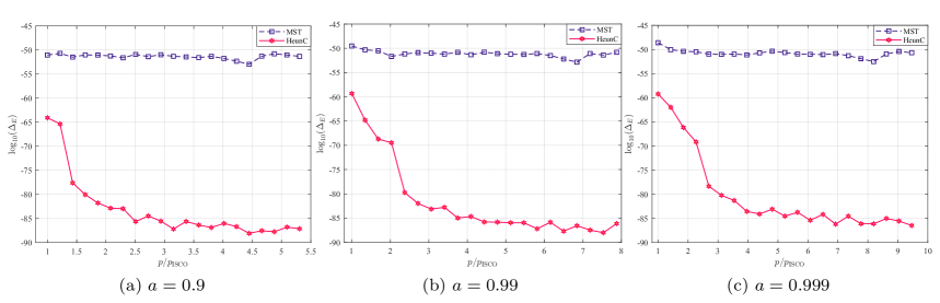
Figure 1: Logarithmic relative errors of radiative fluxes ($\ell_{\rm max}=6$) of circular Orbits at $p=[p_{\rm ISCO},p_{\rm ISCO}+10M]$ with large spins $a=\{0.9,0.99,0.999\}$ and ${\bf{N}}=100$.

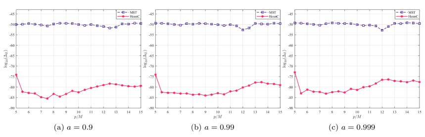
Figure 2: Logarithmic relative errors of radiative fluxes ($\ell_{\rm max}=6$ and $1\leq k\leq 5$) of spherical orbits ($x_{I}=0.9$) at $p=[5M,15M]$ with large spins $a=\{0.9,0.99,0.999\}$ and ${\bf{N}}=100$.

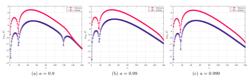
Figure 3: Modal radiative fluxes ($\ell=m=2$) through the horizon and at infinity for the equatorial eccentric orbit ($e=0.9$) at $p=6M$ with large spins $a=\{0.9,0.99,0.999\}$ (To get the data quickly, we set ${\bf{N}}=50$).

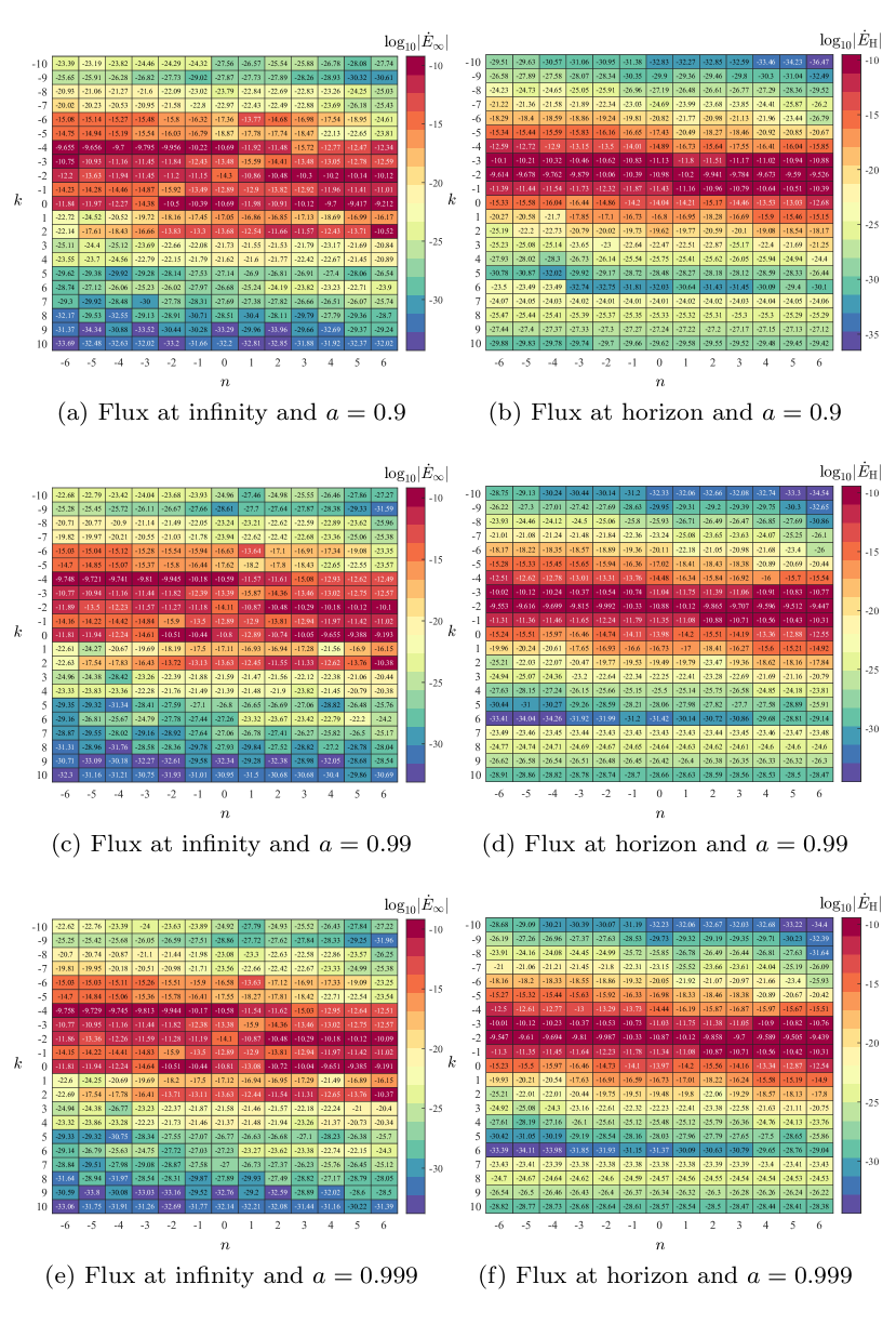
Figure 4: Modal radiative fluxes ($\ell=m=2$) through the horizon and at infinity for the generic Orbit ($e=0.9$ and $x_{I}=0.1$) at $p=10M$ with large spins $a=\{0.9,0.99,0.999\}$ and ${\bf{N}}=50$.

From the above results, it can be seen that the HeunC method has excellent applicability and high precision, and can be used to calculate some extreme cases of general orbits: large eccentricity, higher spin, higher harmonic modes and strong-field regions. When calculating the radiative fluxes of a single higher harmonic mode, it is important to ensure higher floating-point accuracy. The total energy flux, which is obtained by summing thousands of $(\ell,m,k,n)$ modes, plays a crucial role in constructing waveform templates. Our method is capable of achieving higher accuracy using lower floating points, which is advantageous for future efficiency enhancements. Although the MST-NI method exhibits lower efficiency and accuracy compared to the HeunC method when calculating circular orbits, both methods employ the trapezoidal rule for numerical integration in evaluating the integral formulas (3.25) in generic (or eccentric) orbits. The MST-NI method, despite its lower accuracy, surpasses the HeunC method in terms of efficiency. Therefore, to improve the efficiency of the HeunC method, it would be worth exploring the use of a more efficient numerical method for Eq. 3.25.

4.2 Adiabatic inspiral for quasi-circular orbits of non-rotating BH

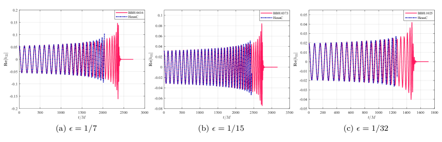
Figure 5: The ‘+’ mode of the stain $h_{22}$ for the different mass ratio binary. Solid red line of data is the RIT waveforms of numerical relativity, and dashed blue line of data is the HeunC method.

After obtaining the data grid of the radiative flux, we can calculate the adiabatic waveform of the inspiral stage by selecting the appropriate orbital evolution equation. In this subsection, the adiabatic inspiral waveform of the dissipative evolution of non-rotating BHs is considered. We use the quasi-circular orbital evolution equation of the adiabatic model [57].

$$\frac{{d\Omega}}{{dt}} =\frac{{d\Omega}}{{d{p}}}{\left({\frac{{dE}}{{d{p}}}}\right)^{-1}}\hat{\nu}{\cal F},$$

$$=\frac{{-3{{\left({{p}-3M}\right)}^{3/2}}}}{{{M^{3/2}}{p}\left({{p}-6M}\right)}}\nu{\cal F},\quad{\cal F}{\rm{=}}-\left({{{\dot{E}}_{\infty}}+{{\dot{E}}_{H}}}\right),$$ (4.2)

$$\frac{{d{\phi_{p}}}}{{dt}} =\Omega,\quad\Omega=\sqrt{M/p^{3}}.$$ (4.3)

where the symmetric mass ratio is $\hat{\nu}={m_{1}}{m_{2}}/{({m_{1}}+{m_{2}})^{2}}$.

According to the selection of the initial boundary conditions, Eqs. 4.2 and 4.3 can be solved to determine $\Omega(t),{\phi_{p}}(t),{p}(t)$. In our applications, we are typically more interested in the waveform $h_{\ell m}(t)$ than in $\psi_{4}(t)$. We give the expression [48, 57] of the waveform $h_{\ell m}(t)$.

$${h_{\ell m}}(t)=\hat{\nu}A_{\ell m}(t){e^{i({m{\phi_{p}}-{\Phi_{0}}})}},$$ (4.4)

where ${\Phi_{0}}$ is the initial phase and the amplitude of the GW waveform is $A_{\ell m}=-{2Z^{\infty}_{\ell m}}/{\omega_{\ell m}^{2}}$.

To obtain $h_{22}$, the grid data of the total energy flux ($\ell_{\rm max}=10$ and ${\bf{N}}=50$) in the region $p=[p_{\rm ISCO},30M]$ is first calculated, with each grid interval set to $\triangle p=0.5M$. The amplitude $A_{22}$ can be extracted from the grid of the total energy flux. By using eighth-order linear interpolation, the values on non-grid points can be efficiently interpolated to obtain a denser grid data with $\triangle p=0.1M$. Subsequently, the adiabatic waveform $h_{22}$ is obtained by substituting the initial boundary conditions of the RIT waveforms [80, 81, 82, 83, 84]. We plot the real part of the waveform for binary systems with different mass ratios in Figure 5. Our waveforms closely match the equivalent waveforms generated by numerical relativity until close to the merger of binary systems.

5 Conclusion

In the previous study [60], the confluent Heun function was utilized to calculate the radiative fluxes resulting from the motion of test particles around a Schwarzschild BH in circular orbits. This paper expands our previous study to obtain the radiative fluxes generated by a particle in generic orbits around a Kerr BH. This extension is effective for considering the gravitational radiation of binary star systems with varying mass ratios. Firstly, we discuss the geodesic dynamics of a point particle on generic orbits in the Kerr spacetime. Then, based on the confluent Heun function, we give the exact solution of Teukolsky equations for the Kerr spacetime. This solution is applied to obtain gravitational wave amplitude and radiative flux. Finally, the radiative flux is used to construct adiabatic inspiral waveforms, and the results are entirely satisfactory in comparison with the analytical and numerical methods. The findings are summarized in detail as follows:

1. From the numerical simulations, it can be seen that the HeunC method has excellent applicability and high precision, and can be used to calculate some extreme cases of general orbits: large eccentricity, higher spin, higher harmonic modes, and strong-field regions. Most frequency domain methods [85, 16, 62] frequently falter in accurately computing GW radiative fluxes in strong-field regions with highly eccentric generic orbits (with eccentricities $e\gtrsim 0.5$). Our method, although belonging to the frequency domain approach, overcomes these computational challenges.

2. The MST method has proven successful in EMRI waveforms calculations, exhibiting incomparable computational accuracy and efficiency [48, 56, 49]. In the case of generic orbits, the calculation of higher harmonic modes requires high floating-point accuracy, because it involves the frequency calculation of four indexes $(\ell,m,k,n)$. As our method undertakes higher floating-point calculations, its accuracy surpasses that of the MST method and high-order post-Newtonian expansion due to the HeunC method’s faster convergence speed. When calculating the radiative fluxes of a single higher harmonic mode, it is important to ensure higher floating-point accuracy. The total energy flux, which is obtained by summing thousands of $(\ell,m,k,n)$ modes, plays a crucial role in constructing waveform templates. Our method is capable of achieving higher accuracy using lower floating points, which is advantageous for efficiency enhancements. This instills confidence in us that the HeunC method will be used for the efficient calculation of GW waveforms in the future.

3. To generate the GW waveform, we use the precomputed frequency-domain Teukolsky equation solutions to obtain the GW radiative fluxes on the orbital grid. In this way, the most computationally expensive aspects of EMRI analysis can be calculated and stored in advance, and then stored data and interpolation techniques are utilized to quickly assemble waveforms. This idea has been successfully validated by Fujita [86] and Hughes [48]. In this paper, we also apply this idea to obtain the adiabatic waveform of the non-rotating BH, which exhibits good agreement with the results of numerical relativity.

Future Plan: To generate waveform data, Hughes et al. used a fairly small internal cluster (about 1000 cores) at the MIT Kavli Institute, which can calculate the inspiral data of 2D orbits (spherical or equatorial), but cannot efficiently calculate the data sets of general 3D orbits (inclined and eccentric Kerr). The calculation framework given in this paper has a lot of room for optimization. How to improve efficiency and reduce CPU time and core number while maintaining high precision of the HeunC method is particularly important. In a companion analysis [87], some of the present authors examined several algorithmic improvements. There are two main aspects: The first improvement is the fast calculation of a single mode. The Green’s function method involves multiple integral formulas (3.28), differential systems of orbital evolution $(p(t^{i}),e(t^{i}),x_{I}(t^{i}))$, and interpolation of non-grid values. This requires the use of some possibly effective numerical algorithms : fast exponential time difference method [88, 89], precise integration method [90, 91], cubic spline interpolation [48] and so on. The challenge of the second improvement arises from the higher dimensionality of the parameter space and the necessity to consider additional modes that contribute to the waveform due to the presence of harmonic frequencies. As the inspirals dig deeper into the strong field, an increased number of modes can significantly impact the waveform. To address these challenges, the framework proposed in Ref. [87] is introduced. The employment of neural network interpolation in this framework shows promise in handling higher dimensions, while the utilization of GPU-based hardware acceleration serves to alleviate the computational burden involved in summing thousands of additional $(\ell,m,k,n)$ modes.

In short, the energy flux grid of the generic orbit proposed in this paper has the advantage of high precision, and its efficiency improvement is what we are committed to doing in the future.

Appendix A Formulas for $E$, $L_{z}$, and $Q$

We provide formulas for the geodesic constants of the motion $(E,L_{z},Q)$ as functions of preferred parameters $(p,e,x_{I})$. The three geodesic constants of generic orbits can be written as

$$E =\sqrt{\frac{\kappa\rho+2\varpi\sigma-2{\rm sgn}(x_{I})\sqrt{\sigma(\sigma\varpi^{2}+\rho\varpi\kappa-\eta\kappa^{2})}}{\rho^{2}+4\eta\sigma}}\;,$$ (A.1)

$$L_{z} =-\frac{g(r_{\rm a})E-\sqrt{g(r_{\rm a})^{2}+h(r_{\rm a})f(r_{\rm a})E^{2}-h(r_{\rm a})d(r_{\rm a})}}{h(r_{\rm a})}\;,$$ (A.2)

$$Q =(1-x_{I}^{2})\left[a^{2}(1-E^{2})+\left(\frac{L_{z}}{x_{I}}\right)^{2}\right]\;,$$ (A.3)

where

$$\kappa =d(r_{\rm a})h(r_{\rm p})-d(r_{\rm p})h(r_{\rm a})\;,$$ (A.4)

$$\varpi =d(r_{\rm a})g(r_{\rm p})-d(r_{\rm p})g(r_{\rm a})\;,$$ (A.5)

$$\rho =f(r_{\rm a})h(r_{\rm p})-f(r_{\rm p})h(r_{\rm a})\;,$$ (A.6)

$$\eta =f(r_{\rm a})g(r_{\rm p})-f(r_{\rm p})g(r_{\rm a})\;,$$ (A.7)

$$\sigma =g(r_{\rm a})h(r_{\rm p})-g(r_{\rm p})h(r_{\rm a})\;,$$ (A.8)

and

$$d(r)= \Delta(r)[r^{2}+a^{2}(1-x_{I}^{2})]\;,$$ (A.9)

$$f(r)= r^{4}+a^{2}[r(r+2M)+(1-x_{I}^{2})\Delta(r)]\;,$$ (A.10)

$$g(r)= 2aMr\;,$$ (A.11)

$$h(r)= r(r-2M)+\frac{(1-x_{I}^{2})\Delta(r)}{x_{I}^{2}}\;,$$ (A.12)

where $r_{\rm a}=p/(1-e)$ and $r_{\rm p}=p/(1+e)$ are the coordinate radius of the orbit’s apoapsis and periapsis, respectively.

More details of these formulas can be seen in Refs. [61, 62]. In addition, we utilized some Hughes’s adjustments [48] for the formula: $\varpi$ replaces $\epsilon$ in Refs. [61, 62] to avoid the symbol conflict with $\epsilon=\sqrt{M^{2}-a^{2}}/2Mr_{+}$ and the very similar $\varepsilon\equiv\mu/M$.

Appendix B Asymptotic Formula of HeunC Function at Infinity

In our previous study [60], we derive the asymptotic analytic expression of the confluent Heun function at infinity. Bonelli et al. solved the connection problem of Heun class functions [92]. By using the connection formulae of $x\in[0,1]$ and $x\in[1,\infty]$ of the confluent Heun function derived by them, the connection formulae of $x\in[0,\infty]$ can be applied to calculate the HeunC value as $x$ tends to infinity. Our analytic expression can also be used to calculate the HeunC value as $x\rightarrow\infty$, and it also contains the amplitude of some physical information. We provide the asymptotic expression of confluent Heun function $\mathbb{H}={\rm{HeunC}}(\alpha,\beta,\gamma,\delta,\eta;x)$ at infinity as follows

$$\mathop{\lim}\limits_{|x|\to\infty}\mathbb{H}(x)=D_{\odot}^{\beta}\;{x^{-\frac{{\beta+\gamma+2}}{2}-\frac{\delta}{\alpha}}}+D_{\otimes}^{\beta}{{\rm{e}}^{-\alpha x}}{x^{-\frac{{\beta+\gamma+2}}{2}+\frac{\delta}{\alpha}}}.$$ (B.1)

Then, the constants $D_{\odot}^{\beta}$ and $D_{\otimes}^{\beta}$ are given by

$$\begin{array}[]{l}D_{\odot}^{\beta}=\Xi_{n,\nu}^{\beta}D_{\odot,n,\nu}^{\beta}+{{\rm{e}}^{-i\pi\left({\nu+\frac{1}{2}}\right)}}\frac{{\sin\pi\left({\nu+\frac{\delta}{\alpha}}\right)}}{{\sin\pi\left({\nu-\frac{\delta}{\alpha}}\right)}}\Xi_{-n,-\nu-1}^{\beta}D_{\odot,-n,-\nu-1}^{\beta},\end{array}$$ (B.3)

$${D_{\otimes}^{\beta}=\Xi_{n,\nu}^{\beta}D_{\otimes,n,\nu}^{\beta}+{{\rm{e}}^{i\pi\left({\nu+\frac{1}{2}}\right)}}\Xi_{-n,-\nu-1}^{\beta}D_{\otimes,-n,-\nu-1}^{\beta},}$$ (B.4)

with

$$D_{\odot,n,\nu}^{\beta} ={\left({-1}\right)^{\frac{{\gamma+\beta+2}}{2}+\frac{\delta}{\alpha}}}{\big{(}{\frac{\alpha}{2}}\big{)}^{\tau}}{\big{(}-{\frac{{i\alpha}}{2}}\big{)}^{-\frac{{\gamma+\beta+2}}{2}-\frac{\delta}{\alpha}}}{{\rm{e}}^{-\frac{{i\pi\tau+\alpha}}{2}}}{2^{-1-\frac{\delta}{\alpha}}}{{\rm{e}}^{\frac{{i\pi}}{2}\big{(}{\nu+1+\frac{\delta}{\alpha}}\big{)}}}\Xi_{n,\nu}^{\beta}\frac{{\Gamma\big{(}{\nu+1+\frac{\delta}{\alpha}}\big{)}}}{{\Gamma\big{(}{\nu+1-\frac{\delta}{\alpha}}\big{)}}},$$ (B.5)

$$D_{\otimes,n,\nu}^{\beta} ={\big{(}{-1}\big{)}^{\frac{{\gamma+\beta+2}}{2}-\frac{\delta}{\alpha}}}{\left({\frac{\alpha}{2}}\right)^{\tau}}{\left(-{\frac{{i\alpha}}{2}}\right)^{-\frac{{\gamma+\beta+2}}{2}+\frac{\delta}{\alpha}}}{{\rm{e}}^{-\frac{{i\pi\tau-\alpha}}{2}}}\Xi_{n,\nu}^{\beta}\frac{{2^{-1+\frac{\delta}{\alpha}}}{{\rm{e}}^{-\frac{{i\pi}}{2}\big{(}{\nu+1-\frac{\delta}{\alpha}}\big{)}}}}{\sum\limits_{n=-\infty}^{+\infty}{f_{n}^{\nu}}}$$

$$\times\Big{(}{\sum\limits_{n=-\infty}^{+\infty}{{{(-1)}^{n}}}\frac{{{{\big{(}{\nu+1-\frac{\delta}{\alpha}}\big{)}}_{n}}}}{{{{\big{(}{\nu+1+\frac{\delta}{\alpha}}\big{)}}_{n}}}}f_{n}^{\nu}}\Big{)}.$$ (B.6)

and

$$\begin{array}[]{*{20}{l}}{\Xi_{n,\nu}^{\beta}=\frac{{{2^{-\nu}}{{\left({\frac{\alpha}{2}}\right)}^{-\hat{\tau}}}{{\rm{e}}^{\frac{{i\pi\hat{\tau}+\alpha}}{2}}}\Gamma\left({\beta+1}\right)\Gamma\left({2\nu+2}\right)}}{{\Gamma\left({\nu+1+\frac{\delta}{\alpha}}\right)\Gamma\left({\nu+1-\frac{{\beta+\gamma}}{2}}\right)\Gamma\left({\nu+1+\frac{{\gamma-\beta}}{2}}\right)}}}\\ {\times{{\Big{(}{\sum\limits_{n=-\infty}^{0}{\frac{{{{(-1)}^{n}}{{\left({\nu+1-\frac{\delta}{\alpha}}\right)}_{n}}}}{{(-n)!{{\left({2\nu+2}\right)}_{n}}{{\left({\nu+1+\frac{\delta}{\alpha}}\right)}_{n}}}}f_{n}^{\nu}}}\Big{)}}^{-1}}}\end{array}$$ (B.9)

$$\begin{array}[]{l}{\times\Big{(}{\sum\limits_{n=0}^{\infty}{{{\left({-1}\right)}^{n}}\frac{{\Gamma\left({n+2\nu+1}\right)\Gamma\left({n+\nu+1+\frac{{\gamma-\beta}}{2}}\right)\Gamma\left({n+\nu+1-\frac{{\beta+\gamma}}{2}}\right)}}{{(n!)\Gamma\left({n+\nu+1+\frac{{\beta-\gamma}}{2}}\right)\Gamma\left({n+\nu+1+\frac{{\beta+\gamma}}{2}}\right)}}f_{n}^{\nu}}}\Big{)}}.\end{array}$$ (B.11)

where $\tau=\frac{1}{4}\left({3\beta+\gamma+\frac{{2\delta}}{\alpha}}\right)$, and $f_{n}^{\nu}$ satisfy the following three-term recurrence relation,

$${{\hat{\alpha}}_{n}}f_{n+1}^{\nu}+{{\hat{\beta}}_{n}}f_{n}^{\nu}+{{\hat{\gamma}}_{n}}f_{n-1}^{\nu}=0,$$ (B.12)

where

$${{\hat{\alpha}}_{n}} =\frac{{\left({2n+2\nu+2-\beta+\gamma}\right)}}{{8\left({n+\nu+1}\right)\left({2n+2\nu+3}\right)}}\left({\alpha n+\alpha\nu+\alpha-\delta}\right)\left({2n+2\nu+2-\gamma-\beta}\right),$$ (B.13a)

$${{\hat{\beta}}_{n}} =\eta+\frac{\delta}{2}-\frac{{{\beta^{2}}}}{4}-\frac{{{\gamma^{2}}}}{4}+\left({n+\nu}\right)\left({n+\nu+1}\right)+\frac{{\delta\left({\gamma+\beta}\right)\left({\beta-\gamma}\right)}}{{8\left({n+\nu}\right)\left({n+\nu+1}\right)}},$$ (B.13b)

$${{\hat{\gamma}}_{n}} =-\frac{{\left({2n+2\nu+\beta-\gamma}\right)}}{{8\left({n+\nu}\right)\left(2n+2\nu-1\right)}}\left({\alpha n+\alpha\nu+\delta}\right)\left({2n+2\nu+\gamma+\beta}\right).$$ (B.13c)

The phase parameter $\nu$, also known as the renormalized angular momentum, may be obtained by solving a characteristic equation expressed as the sum of two infinite continued fractions.

$${{\hat{\beta}}_{0}}=\frac{{{{\hat{\alpha}}_{-1}}{{\hat{\gamma}}_{0}}}}{{{{\hat{\beta}}_{-1}}-}}\frac{{{{\hat{\alpha}}_{-2}}{{\hat{\gamma}}_{-1}}}}{{{{\hat{\beta}}_{-2}}-}}\frac{{{{\hat{\alpha}}_{-3}}{{\hat{\gamma}}_{-2}}}}{{{{\hat{\beta}}_{-3}}-}}+\cdots+\frac{{{{\hat{\alpha}}_{0}}{{\hat{\gamma}}_{1}}}}{{{{\hat{\beta}}_{1}}-}}\frac{{{{\hat{\alpha}}_{1}}{{\hat{\gamma}}_{2}}}}{{{{\hat{\beta}}_{2}}-}}\frac{{{{\hat{\alpha}}_{2}}{{\hat{\gamma}}_{3}}}}{{{{\hat{\beta}}_{3}}-}}\cdots.$$ (B.14)

Appendix C Parameters of HeunC Functions

Currently, the three primary mathematical software packages offer numerical calculation capabilities for the confluent Heun function, as well as for its derivation and integration. MAPLE and Mathematica provide official built-in functions for these calculations, while the calculation code of MATLAB is provided by Motygin [93, 94].

For Maple software, the ODE of the confluent Heun function $\mathbb{H}_{\rm{0}}^{\beta}(x)={\rm{HeunC}}(\alpha,\beta,\gamma,\delta,\eta;x)$ can be written as

$$\mathbb{H}^{\prime\prime}-\frac{{\left({-{x^{2}}\alpha+\left({-2-\beta-\gamma+\alpha}\right)x+1+\beta}\right)}}{{x\left({x-1}\right)}}\mathbb{H}^{\prime}$$

$$-\left[\left({\left({-2-\beta-\gamma}\right)\alpha-2\delta}\right)x+\left({\beta+1}\right)\alpha+\left({-\gamma-1}\right)\beta-\gamma-2\eta\right]\frac{\mathbb{H}}{{2x\left({x-1}\right)}}=0.$$ (C.1)

For MATLAB/Mathematica software, the ODE of the confluent Heun function can be written as

$${\bf{H^{\prime\prime}}}+{\bf{H^{\prime}}}\left({\frac{{{\gamma_{\rm{M}}}}}{x}+\frac{{{\delta_{\rm{M}}}}}{{x-1}}+{\epsilon_{\rm{M}}}}\right)+\frac{{({\alpha_{\rm{M}}}x-{q_{\rm{M}}})}}{{x(x-1)}}{\bf{H}}=0$$ (C.2)

where ${\bf{H}}(x)={\rm{HeunC}}({q_{\rm{M}}},{\alpha_{\rm{M}}},{\gamma_{\rm{M}}},{\delta_{\rm{M}}},{\epsilon_{\rm{M}}};x)$.

The parameter relation between Appendix C and C.2 is as follows

$${q_{{\rm{M}}}} =\frac{1}{2}\alpha\beta-\frac{1}{2}\beta\gamma+\frac{1}{2}\alpha-\frac{1}{2}\beta-\eta-\frac{1}{2}\gamma,$$ (C.3a)

$${\alpha_{{\rm{M}}}} =\frac{1}{2}\alpha\beta+\frac{1}{2}\alpha\gamma+\alpha+\delta,$$ (C.3b)

$${\delta_{{\rm{M}}}} =\gamma+1,$$ (C.3c)

$${\epsilon_{{\rm{M}}}} =\alpha,$$ (C.3d)

$${\gamma_{{\rm{M}}}} =\beta+1.$$ (C.3e)

References

- [1] LIGO Scientific, Virgo collaboration, Improved analysis of GW150914 using a fully spin-precessing waveform Model, Phys. Rev. X 6 (2016) 041014 [1606.01210].
- [2] LIGO Scientific, Virgo collaboration, Binary Black Hole Mergers in the first Advanced LIGO Observing Run, Phys. Rev. X 6 (2016) 041015 [1606.04856].
- [3] LIGO Scientific, Virgo collaboration, GWTC-1: A Gravitational-Wave Transient Catalog of Compact Binary Mergers Observed by LIGO and Virgo during the First and Second Observing Runs, Phys. Rev. X 9 (2019) 031040 [1811.12907].
- [4] LIGO Scientific, Virgo collaboration, GWTC-2: Compact Binary Coalescences Observed by LIGO and Virgo During the First Half of the Third Observing Run, Phys. Rev. X 11 (2021) 021053 [2010.14527].
- [5] KAGRA, VIRGO, LIGO Scientific collaboration, Population of Merging Compact Binaries Inferred Using Gravitational Waves through GWTC-3, Phys. Rev. X 13 (2023) 011048 [2111.03634].
- [6] LISA collaboration, Laser Interferometer Space Antenna, 1702.00786.
- [7] LISA Consortium Waveform Working Group collaboration, Waveform Modelling for the Laser Interferometer Space Antenna, 2311.01300.
- [8] TianQin collaboration, TianQin: a space-borne gravitational wave detector, Class. Quant. Grav. 33 (2016) 035010 [1512.02076].
- [9] TianQin collaboration, The TianQin project: current progress on science and technology, PTEP 2021 (2021) 05A107 [2008.10332].
- [10] W.-H. Ruan, Z.-K. Guo, R.-G. Cai and Y.-Z. Zhang, Taiji program: Gravitational-wave sources, Int. J. Mod. Phys. A 35 (2020) 2050075 [1807.09495].
- [11] S. Babak, J. Gair, A. Sesana, E. Barausse, C.F. Sopuerta, C.P.L. Berry et al., Science with the space-based interferometer LISA. V: Extreme mass-ratio inspirals, Phys. Rev. D 95 (2017) 103012 [1703.09722].
- [12] Y. Mino, M. Sasaki and T. Tanaka, Gravitational radiation reaction to a particle motion, Phys. Rev. D 55 (1997) 3457 [gr-qc/9606018].
- [13] T.C. Quinn and R.M. Wald, An Axiomatic approach to electromagnetic and gravitational radiation reaction of particles in curved space-time, Phys. Rev. D 56 (1997) 3381 [gr-qc/9610053].
- [14] L. Barack, Gravitational self force in extreme mass-ratio inspirals, Class. Quant. Grav. 26 (2009) 213001 [0908.1664].
- [15] E. Poisson, A. Pound and I. Vega, The Motion of point particles in curved spacetime, Living Rev. Rel. 14 (2011) 7 [1102.0529].
- [16] B. Wardell, Self-force: Computational Strategies, Fund. Theor. Phys. 179 (2015) 487 [1501.07322].
- [17] A. Pound, Motion of small objects in curved spacetimes: An introduction to gravitational self-force, Fund. Theor. Phys. 179 (2015) 399 [1506.06245].
- [18] A. Pound and B. Wardell, Black hole perturbation theory and gravitational self-force, 2101.04592.
- [19] S.A. Teukolsky, Rotating black holes - separable wave equations for gravitational and electromagnetic perturbations, Phys. Rev. Lett. 29 (1972) 1114.
- [20] S.A. Teukolsky, Perturbations of a rotating black hole. 1. Fundamental equations for gravitational electromagnetic and neutrino field perturbations, Astrophys. J. 185 (1973) 635.
- [21] W.H. Press and S.A. Teukolsky, Perturbations of a Rotating Black Hole. II. Dynamical Stability of the Kerr Metric, Astrophys. J. 185 (1973) 649.
- [22] S.A. Teukolsky and W.H. Press, Perturbations of a rotating black hole. III - Interaction of the hole with gravitational and electromagnet ic radiation, Astrophys. J. 193 (1974) 443.
- [23] R.M. Wald, On perturbations of a Kerr black hole, J. Math. Phys. 14 (1973) 1453.
- [24] J.M. Cohen and L.S. Kegeles, Electromagnetic fields in curved spaces - a constructive procedure, Phys. Rev. D 10 (1974) 1070.
- [25] P.L. Chrzanowski, Vector Potential and Metric Perturbations of a Rotating Black Hole, Phys. Rev. D 11 (1975) 2042.
- [26] L.S. Kegeles and J.M. Cohen, CONSTRUCTIVE PROCEDURE FOR PERTURBATIONS OF SPACE-TIMES, Phys. Rev. D 19 (1979) 1641.
- [27] A. Ori, Reconstruction of inhomogeneous metric perturbations and electromagnetic four potential in Kerr space-time, Phys. Rev. D 67 (2003) 124010 [gr-qc/0207045].
- [28] A. Pound, C. Merlin and L. Barack, Gravitational self-force from radiation-gauge metric perturbations, Phys. Rev. D 89 (2014) 024009 [1310.1513].
- [29] T.S. Keidl, J.L. Friedman and A.G. Wiseman, On finding fields and self-force in a gauge appropriate to separable wave equations, Phys. Rev. D 75 (2007) 124009 [gr-qc/0611072].
- [30] T.S. Keidl, A.G. Shah, J.L. Friedman, D.-H. Kim and L.R. Price, Gravitational Self-force in a Radiation Gauge, Phys. Rev. D 82 (2010) 124012 [1004.2276].
- [31] A.G. Shah, T.S. Keidl, J.L. Friedman, D.-H. Kim and L.R. Price, Conservative, gravitational self-force for a particle in circular orbit around a Schwarzschild black hole in a Radiation Gauge, Phys. Rev. D 83 (2011) 064018 [1009.4876].
- [32] A.G. Shah, J.L. Friedman and T.S. Keidl, EMRI corrections to the angular velocity and redshift factor of a mass in circular orbit about a Kerr black hole, Phys. Rev. D 86 (2012) 084059 [1207.5595].
- [33] M. van de Meent and A.G. Shah, Metric perturbations produced by eccentric equatorial orbits around a Kerr black hole, Phys. Rev. D 92 (2015) 064025 [1506.04755].
- [34] M. van de Meent, Self-force corrections to the periapsis advance around a spinning black hole, Phys. Rev. Lett. 118 (2017) 011101 [1610.03497].
- [35] M. van de Meent, Gravitational self-force on generic bound geodesics in Kerr spacetime, Phys. Rev. D 97 (2018) 104033 [1711.09607].
- [36] C. Merlin, A. Ori, L. Barack, A. Pound and M. van de Meent, Completion of metric reconstruction for a particle orbiting a Kerr black hole, Phys. Rev. D 94 (2016) 104066 [1609.01227].
- [37] M. van De Meent, The mass and angular momentum of reconstructed metric perturbations, Class. Quant. Grav. 34 (2017) 124003 [1702.00969].
- [38] T. Hinderer and E.E. Flanagan, Two timescale analysis of extreme mass ratio inspirals in Kerr. I. Orbital Motion, Phys. Rev. D 78 (2008) 064028 [0805.3337].
- [39] E.E. Flanagan and T. Hinderer, Transient resonances in the inspirals of point particles into black holes, Phys. Rev. Lett. 109 (2012) 071102 [1009.4923].
- [40] Y. Mino, Perturbative approach to an orbital evolution around a supermassive black hole, Phys. Rev. D 67 (2003) 084027 [gr-qc/0302075].
- [41] N. Sago, T. Tanaka, W. Hikida, K. Ganz and H. Nakano, The Adiabatic evolution of orbital parameters in the Kerr spacetime, Prog. Theor. Phys. 115 (2006) 873 [gr-qc/0511151].
- [42] T. Osburn, E. Forseth, C.R. Evans and S. Hopper, Lorenz gauge gravitational self-force calculations of eccentric binaries using a frequency domain procedure, Phys. Rev. D 90 (2014) 104031 [1409.4419].
- [43] M. Sasaki and T. Nakamura, The regge-wheeler equation with sources for both even and odd parity perturbations of the schwarzschild geometry, Phys. Lett. A 87 (1981) 85.
- [44] S.A. Hughes, The Evolution of circular, nonequatorial orbits of Kerr black holes due to gravitational wave emission, Phys. Rev. D 61 (2000) 084004 [gr-qc/9910091].
- [45] S.A. Hughes, Evolution of circular, nonequatorial orbits of Kerr black holes due to gravitational wave emission. II. Inspiral trajectories and gravitational wave forms, Phys. Rev. D 64 (2001) 064004 [gr-qc/0104041].
- [46] S. Drasco and S.A. Hughes, Rotating black hole orbit functionals in the frequency domain, Phys. Rev. D 69 (2004) 044015 [astro-ph/0308479].
- [47] S. Drasco and S.A. Hughes, Gravitational wave snapshots of generic extreme mass ratio inspirals, Phys.Rev.D 73 (2006) 024027 [gr-qc/0509101].
- [48] S.A. Hughes, N. Warburton, G. Khanna, A.J.K. Chua and M.L. Katz, Adiabatic waveforms for extreme mass-ratio inspirals via multivoice decomposition in time and frequency, Phys. Rev. D 103 (2021) 104014 [2102.02713].
- [49] V. Skoupy, G. Lukes-Gerakopoulos, L.V. Drummond and S.A. Hughes, Asymptotic gravitational-wave fluxes from a spinning test body on generic orbits around a Kerr black hole, Phys. Rev. D 108 (2023) 044041 [2303.16798].
- [50] L.V. Drummond and S.A. Hughes, Precisely computing bound orbits of spinning bodies around black holes. I. General framework and results for nearly equatorial orbits, Phys. Rev. D 105 (2022) 124040 [2201.13334].
- [51] L.V. Drummond and S.A. Hughes, Precisely computing bound orbits of spinning bodies around black holes. II. Generic orbits, Phys. Rev. D 105 (2022) 124041 [2201.13335].
- [52] R. Fujita, W. Hikida and H. Tagoshi, An Efficient Numerical Method for Computing Gravitational Waves Induced by a Particle Moving on Eccentric Inclined Orbits around a Kerr Black Hole, Prog. Theor. Phys. 121 (2009) 843 [0904.3810].
- [53] R. Fujita and W. Hikida, Analytical solutions of bound timelike geodesic orbits in Kerr spacetime, Class. Quant. Grav. 26 (2009) 135002 [0906.1420].
- [54] N. Sago and R. Fujita, Calculation of radiation reaction effect on orbital parameters in Kerr spacetime, PTEP 2015 (2015) 073E03 [1505.01600].
- [55] R. Fujita and M. Shibata, Extreme mass ratio inspirals on the equatorial plane in the adiabatic order, Phys. Rev. D 102 (2020) 064005 [2008.13554].
- [56] S. Isoyama, R. Fujita, A.J.K. Chua, H. Nakano, A. Pound and N. Sago, Adiabatic Waveforms from Extreme-Mass-Ratio Inspirals: An Analytical Approach, Phys. Rev. Lett. 128 (2022) 231101 [2111.05288].
- [57] B. Wardell, A. Pound, N. Warburton, J. Miller, L. Durkan and A. Le Tiec, Gravitational Waveforms for Compact Binaries from Second-Order Self-Force Theory, Phys. Rev. Lett. 130 (2023) 241402 [2112.12265].
- [58] C. Zhang, Y. Gong, D. Liang and B. Wang, Gravitational waves from eccentric extreme mass-ratio inspirals as probes of scalar fields, JCAP 06 (2023) 054 [2210.11121].
- [59] C. Zhang, H. Guo, Y. Gong and B. Wang, Detecting vector charge with extreme mass ratio inspirals onto Kerr black holes, JCAP 06 (2023) 020 [2301.05915].
- [60] C. Chen and J. Jing, Radiation fluxes of gravitational, electromagnetic, and scalar perturbations in type-D black holes: an exact approach, JCAP 11 (2023) 070 [2307.14616].
- [61] W. Schmidt, Celestial mechanics in Kerr space-time, Class. Quant. Grav. 19 (2002) 2743 [gr-qc/0202090].
- [62] M. van de Meent, Analytic solutions for parallel transport along generic bound geodesics in Kerr spacetime, Class. Quant. Grav. 37 (2020) 145007 [1906.05090].
- [63] M. Sasaki and H. Tagoshi, Analytic black hole perturbation approach to gravitational radiation, Living Rev. Rel. 6 (2003) 6 [gr-qc/0306120].
- [64] S. O’Sullivan and S.A. Hughes, Strong-field tidal distortions of rotating black holes: Formalism and results for circular, equatorial orbits, Phys. Rev. D 90 (2014) 124039 [1407.6983].
- [65] H. Tagoshi and M. Sasaki, Post-Newtonian expansion of gravitational waves from a particle in circular orbit around a Schwarzschild black hole, Prog. Theor. Phys. 92 (1994) 745 [gr-qc/9405062].
- [66] H. Tagoshi, M. Shibata, T. Tanaka and M. Sasaki, Post-Newtonian expansion of gravitational waves from a particle in circular orbits around a rotating black hole: Up to O () beyond the quadrupole formula, Phys. Rev. D 54 (1996) 1439 [gr-qc/9603028].
- [67] T. Tanaka, H. Tagoshi and M. Sasaki, Gravitational waves by a particle in circular orbits around a Schwarzschild black hole: 5.5 post-Newtonian formula, Prog. Theor. Phys. 96 (1996) 1087 [gr-qc/9701050].
- [68] M. Shibata, M. Sasaki, H. Tagoshi and T. Tanaka, Gravitational waves from a particle orbiting around a rotating black hole: Post-Newtonian expansion, Phys. Rev. D 51 (1995) 1646 [gr-qc/9409054].
- [69] S. Mano, H. Suzuki and E. Takasugi, Analytic solutions of the Regge-Wheeler equation and the post-Minkowskian expansion, Prog. Theor. Phys. 96 (1996) 549 [gr-qc/9605057].
- [70] S. Mano, H. Suzuki and E. Takasugi, Analytic solutions of the Teukolsky equation and their low frequency expansions, Prog. Theor. Phys. 95 (1996) 1079 [gr-qc/9603020].
- [71] A. Ronveaux and F.M. Arscott, Heun’s differential equations, Oxford University Press (1995).
- [72] S. Slavyanov and W. Lay, Special Functions: Unified Theory Based on Singularities, Oxford University Press (2000).
- [73] F.W. Olver, D.W. Lozier, R.F. Boisvert and C.W. Clark, NIST handbook of mathematical functions hardback and CD-ROM, Cambridge university press (2010).
- [74] R. Fujita, Gravitational Waves from a Particle in Circular Orbits around a Rotating Black Hole to the 11th Post-Newtonian Order, PTEP 2015 (2015) 033E01 [1412.5689].
- [75] “Black Hole Perturbation Toolkit.” (bhptoolkit.org), 2023.
- [76] R. Fujita and H. Tagoshi, New numerical methods to evaluate homogeneous solutions of the Teukolsky equation, Prog. Theor. Phys. 112 (2004) 415 [gr-qc/0410018].
- [77] R. Fujita and H. Tagoshi, New Numerical Methods to Evaluate Homogeneous Solutions of the Teukolsky Equation II. Solutions of the Continued Fraction Equation, Prog. Theor. Phys. 113 (2005) 1165 [0904.3818].
- [78] L. Barack and C. Cutler, LISA capture sources: Approximate waveforms, signal-to-noise ratios, and parameter estimation accuracy, Phys. Rev. D 69 (2004) 082005 [gr-qc/0310125].
- [79] J.R. Gair, L. Barack, T. Creighton, C. Cutler, S.L. Larson, E.S. Phinney et al., Event rate estimates for LISA extreme mass ratio capture sources, Class. Quant. Grav. 21 (2004) S1595 [gr-qc/0405137].
- [80] J. Healy, C.O. Lousto, Y. Zlochower and M. Campanelli, The RIT binary black hole simulations catalog, Class. Quant. Grav. 34 (2017) 224001 [1703.03423].
- [81] J. Healy, C.O. Lousto, J. Lange, R. O’Shaughnessy, Y. Zlochower and M. Campanelli, Second RIT binary black hole simulations catalog and its application to gravitational waves parameter estimation, Phys. Rev. D 100 (2019) 024021 [1901.02553].
- [82] J. Healy and C.O. Lousto, Third RIT binary black hole simulations catalog, Phys. Rev. D 102 (2020) 104018 [2007.07910].
- [83] J. Healy and C.O. Lousto, Fourth RIT binary black hole simulations catalog: Extension to eccentric orbits, Phys. Rev. D 105 (2022) 124010 [2202.00018].
- [84] “RIT Waveform Catalog .” (RITCatalog), 2023.
- [85] J.L. Barton, D.J. Lazar, D.J. Kennefick, G. Khanna and L.M. Burko, Computational Efficiency of Frequency and Time-Domain Calculations of Extreme Mass-Ratio Binaries: Equatorial Orbits, Phys. Rev. D 78 (2008) 064042 [0804.1075].
- [86] R. Fujita and M. Shibata, Extreme mass ratio inspirals on the equatorial plane in the adiabatic order, Phys. Rev. D 102 (2020) 064005 [2008.13554].
- [87] A.J.K. Chua, M.L. Katz, N. Warburton and S.A. Hughes, Rapid generation of fully relativistic extreme-mass-ratio-inspiral waveform templates for LISA data analysis, Phys. Rev. Lett. 126 (2021) 051102 [2008.06071].
- [88] J. Huang, L. Ju and B. Wu, A fast compact time integrator method for a family of general order semilinear evolution equations, J. Comput. Phys. 393 (2019) 313.
- [89] M. Hederi, A. Islas, K. Reger and C. Schober, Efficiency of exponential time differencing schemes for nonlinear schrödinger equations, Math. Comput. Simul. 127 (2016) 101.
- [90] W. Zhong, Combined method for the solution of asymmetric riccati differential equations, Comput. Methods Appl. Mech. Eng. 191 (2001) 93.
- [91] C. Chen, X. Zhang, Z. Liu and Y. Zhang, A new high-order compact finite difference scheme based on precise integration method for the numerical simulation of parabolic equations, Adv. Diff. Eq. 2020 (2020) 1.
- [92] G. Bonelli, C. Iossa, D. Panea Lichtig and A. Tanzini, Irregular Liouville Correlators and Connection Formulae for Heun Functions, Commun. Math. Phys. 397 (2023) 635 [2201.04491].
- [93] O.V. Motygin, On numerical evaluation of the Heun functions, in 2015 Days on Diffraction (DD), IEEE, may, 2015, DOI.
- [94] O.V. Motygin, On evaluation of the confluent Heun functions, in 2018 Days on Diffraction (DD), IEEE, 2018, DOI.