Optimize the event selection strategy the study the anomalous quartic gauge couplings at muon colliders using the support vector machine

Abstract

The search of the new physics (NP) beyond the Standard Model is one of the most important topics in current high energy physics research. With the increasing luminosities at the colliders, the search for NP signals requires the analysis of more and more data, and the efficiency in data processing becomes particularly important. As a machine learning algorithm, the support vector machine (SVM) is expected to be useful in the search of NP, meanwhile, has the potential to be accelerated with the help of quantum computing. How to use the SVM to optimize an event selection strategy to search for NP signals is studied in this paper. Taking the tri-photon process at a muon collider as an example, it can be shown that the event selection strategy optimized by the SVM is effective in the search of the dimension-8 operators contributing to the anomalous quartic gauge couplings.

I Introduction

At present, the Standard Model (SM) has been remarkably successful. However, it still faces many unsolved mysteries and limitations. The SM cannot explain phenomena such as dark matter, the unification of gravity with quantum mechanics, and other unresolved questions. Searching for new physics (NP) can help explain these mysteries and fill the gaps in the SM. Moreover, the search of NP has become one of the frontiers in high energy physics (HEP) [1] research. As future colliders continuously increase their designed luminosities, high-luminosity colliders not only enhance the chances of searching NP signals but also demand higher efficiency in detecting NP signals.

One way to explore NP efficiently is to use the SM Effective Field Theory (SMEFT) to explore possible NP signals [2, 3, 4, 5]. SMEFT primarily focuses on dimension-6 operators. However, from a phenomenological point of view, there are many cases where dimension-6 operators are absent, but the dimension-8 operators show up [6, 7, 8, 8, 9, 10, 11, 12, 13, 14, 15]. And the dimension-8 operators are important w.r.t. the convex geometry perspective to the operator space. Therefore, in this paper, we study dimension-8 operators contributing to anomalous quartic gauge couplings (aQGCs). In addition, with the increasing energy and luminosity at the Large Harden Collider (LHC), the LHC has maintained a close interest in dimension-8 operators [16, 17, 18, 19, 20, 21, 22, 23, 24, 25, 26, 27, 28, 29, 30]. Phenomenological studies on aQGCs is also being conducted intensively [31, 32, 33, 34, 35, 36, 37, 38]. However, for one generation of fermions, there are $895$ baryon number conserving dimension-8 operators [39, 33], and kinematic analysis needs to be done for each operator. The efficiency decreases with the growth of the number of operators to be considered.

In recent years, machine learning algorithms (ML) have experienced rapid development in the field of HEP [40, 41, 42, 43, 44, 45, 46, 47, 48, 49, 50, 51]. From a ML perspective, searching for NP signals can be viewed as anomaly detection [52, 50, 51, 53, 54, 55, 56, 57, 58, 59]. In addition to this, discriminating between NP signal events and background events can be viewed as a classification problem, and there exists a large number of classification algorithms available for use in ML. In this paper, we will explore a commonly used classification algorithm, the support vector machines (SVM). One of the major advantages of using machine learning is that, usually it does not require the knowledge of the NP model, but simply follows the steps of the algorithm to automate the results.

It is widely acknowledged that quantum computer can be used to speed up computation. Researchers have already explored the application of SVM on quantum computer, resulting in the development of the quantum support vector machine (QSVM). QSVM takes advantage of quantum computing properties, such as quantum superposition and quantum entanglement, to expedite the solution of SVM problems [60, 61, 62, 63]. While the SVM is well-suited for data classification [64], its potential for searching for NP remains uncertain, this is due to the fact that algorithms for classification problems are not always suitable for anomaly detection, the latter being concerned with situations where it is equivalent to categorizing two classes that are very different in number. In this paper, we focus on investigating the feasibility of using the SVM to search for NP. In particular, how an event selection strategy can be optimized using the SVM is studied.

Recently, there has been increasing interest in muon colliders, as they offer the potential to reach high energies and high luminosities while providing a cleaner experimental environment with less impact from QCD backgrounds than the hadron colliders [65, 66, 67, 68, 69, 70, 71, 72, 73, 74]. As a testing ground, we take the tri-photon process at a muon collider to study the aQGCs and optimize an event selection strategy to search for signals of aQGCs while imposing constraints on the operator coefficients using the SVM. The tri-photon process at a muon collider is chosen because it is considered to be particularly sensitive to the transverse operators contributing to the aQGCs [75], and is therefore a process worth investigating. It is worth mentioning that, as a ML algorithm, the expected procedure of optimizing the event selection strategy using the SVM does not depend on the process to be studied.

The remaining of this paper are structured as follows, in Section II, we provide a brief introduction to the aQGCs and the tri-photon process. Section III discusses the event selection strategy utilizing the SVM. The expected constraints on the operator coefficients are presented in section IV. Section V summarizes the main conclusions.

II aQGCs and tri-photon process at the muon colliders

coefficient	constraint	coefficient	constraint
$f_{T_{0}}/\Lambda^{4}$	[$-0.12,0.11$] [28]	$f_{T_{6}}/\Lambda^{4}$	[$-0.4,0.4$] [29]
$f_{T_{1}}/\Lambda^{4}$	[$-0.12,0.13$] [28]	$f_{T_{7}}/\Lambda^{4}$	[$-0.9,0.9$] [29]
$f_{T_{2}}/\Lambda^{4}$	[$-0.28,0.28$] [28]	$f_{T_{8}}/\Lambda^{4}$	[$-0.43,0.43$] [30]
$f_{T_{5}}/\Lambda^{4}$	[$-0.5,0.5$] [29]	$f_{T_{9}}/\Lambda^{4}$	[$-0.92,0.92$] [30]

Table 1: The expected constraints on the $O_{T_{i}}$ coefficients obtained at $95~{}\%$ C.L. at the LHC.

In previous studies, the dimension-8 operators contributing to the aQGCs can be classified as scalar/longitudinal operators $O_{S_{i}}$, mixed transverse and longitudinal operators $O_{M_{i}}$ and transverse operators $O_{T_{i}}$ [76]. In this paper we focus on $O_{T_{i}}$ operators [77, 78], which contribute to tri-photon process at muon colliders. They are,

$$\begin{split}&O_{T,0}={\rm Tr}\left[\widehat{W}_{\mu\nu}\widehat{W}^{\mu\nu}\right]\times{\rm Tr}\left[\widehat{W}_{\alpha\beta}\widehat{W}^{\alpha\beta}\right],\\ &O_{T,2}={\rm Tr}\left[\widehat{W}_{\alpha\mu}\widehat{W}^{\mu\beta}\right]\times{\rm Tr}\left[\widehat{W}_{\beta\nu}\widehat{W}^{\nu\alpha}\right],\\ &O_{T,6}={\rm Tr}\left[\widehat{W}_{\alpha\nu}\widehat{W}^{\mu\beta}\right]\times B_{\mu\beta}B^{\alpha\nu},\\ &O_{T,8}=B_{\mu\nu}B^{\mu\nu}\times B_{\alpha\beta}B^{\alpha\beta},\\ \end{split}\quad\begin{split}&O_{T,1}={\rm Tr}\left[\widehat{W}_{\alpha\nu}\widehat{W}^{\mu\beta}\right]\times{\rm Tr}\left[\widehat{W}_{\mu\beta}\widehat{W}^{\alpha\nu}\right],\\ &O_{T,5}={\rm Tr}\left[\widehat{W}_{\mu\nu}\widehat{W}^{\mu\nu}\right]\times B_{\alpha\beta}B^{\alpha\beta},\\ &O_{T,7}={\rm Tr}\left[\widehat{W}_{\alpha\mu}\widehat{W}^{\mu\beta}\right]\times B_{\beta\nu}B^{\nu\alpha},\\ &O_{T,9}=B_{\alpha\mu}B^{\mu\beta}\times B_{\beta\nu}B^{\nu\alpha},\\ \end{split}$$ (1)

where $\widehat{W}\equiv\vec{\sigma}\cdot{\vec{W}}/2$ with $\sigma$ being the Pauli matrices and ${\vec{W}}=\{W^{1},W^{2},W^{3}\}$, $B_{\mu}$ and $W_{\mu}^{i}$ are $U(1)_{\rm Y}$ and $SU(2)_{\rm I}$ gauge fields, and $B_{\mu\nu}$ and $W_{\mu\nu}$ correspond to the field strength tensors. Table 1 presents the constraints obtained at the LHC on the coefficients of the dimension-8 operators.

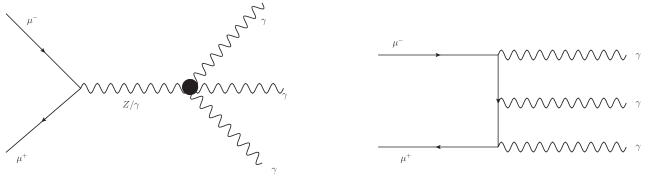
Figure 1: Feynman diagrams for the tri-photon processes $\mu^{+}\mu^{-}\rightarrow\gamma\gamma\gamma$ . The left panel shows the diagrams induced by $O_{T_{i}}$, while the right panel is one of the diagrams in SM. In the SM, there are five additional diagrams that can be obtained by permuting the photons in the final state.

For the process $\mu^{+}\mu^{-}\to\gamma\gamma\gamma$, the diagrams induced by $O_{T_{i}}$ operators are shown on the left panel of Fig. 1, and the right panel of Fig. 1 shows one of the diagrams in the SM. In the SM, there are other five diagrams that can be obtained by permuting the photons in the final state. The expressions for the contributions of the $O_{T_{i}}$ operators and the interference between $O_{T_{i}}$ operators and the SM are given in Ref. [75], it is shown that the contributions of $O_{T_{1,6}}$ operators are exactly as same as $O_{T_{0,5}}$ operators. Therefore, we concentrate on $O_{T_{0,2,5,7,8,9}}$ operators in the following.

III Event selection strategy

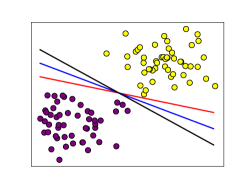
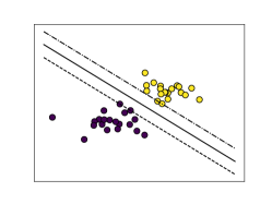
Figure 2: The left panel shows the classification of linearly divisible data points in a 2-dimensional space by using an ordinary method. The middle panel shows their classification by using the SVM. In the right panel, the SVM is used to distinguish the data points in 2-dimensional space which are linearly indivisible.

In general, the search for the NP signals at the colliders with high luminosities is to look for a small number of anomalies in a vast amount of experimental data. This is a binary classification problem that distinguish the NP events from the SM background. One of the ML algorithms designed for the binary classification problem is the SVM. Therefore, it can be expected that the SVM can be used to search for NP signals.

As shown in the left panel of Fig. 2, we take the example of two types of linearly divisible data points in a 2-dimensional space. We can make arbitrary divisions and give different division lines according to the different classes of elements in the data set. But we can’t identify the line with the best classification. SVM makes up for this by automatically identifying the line of division (the line of division is the hyperplane in the SVM algorithm), which is the furthest away from the two types of data points, as shown in the center of Fig. 2. Moreover, when the data set is linearly indivisible, the SVM can automatically find the classification line that simultaneously maximizes the minimum distance between the two point sets, and separates the two point sets as far as possible, as shown in the right panel of Fig. 2.

In particular, a collision event can be represented as a point in a multidimensional space, where each dimension corresponds to an observable in the measurement (denoted as $M_{i}$) associated with that collision event. Traditional event selection strategies typically use intervals for segmentation, i.e., retaining or excluding events with $M_{i}^{\rm min}<M_{i}<M_{i}^{\rm max}$. This is equivalent to selecting or excluding a hyper cuboid in the multidimensional space described above. Unlike the traditional approach, if we use the SVM algorithm for the event selection strategy, we will automatically get a hyperplane that separates the NP from the SM in the above multidimensional space. This hyperplane corresponds to a criterion consisting of $M_{i}$, so similar to the traditional event selection strategy, it is also a set of strategies consisting of observables. Because SVM can automatically find the hyperplane that best separates the two types of events, the event selection strategy obtained by the SVM can be viewed as an optimization of a traditional one. It should be emphasized that, the collection of observables requires no knowledge of the NP model at all, but only a sufficiently large number of observables based on the final state to be selected.

Another similar approach to optimize the event select strategy automatically is to use the decision tree, which is also an algorithm used for classification [79, 80, 81]. With continuous improvement of the algorithms, decision tree and algorithms derived from the decision trees are widely used in HEP, including the searching of NP signals [82, 83, 84]. To use the SVM is similar, however with a different algorithm. Since there is no a-priori superiority for any classification algorithm over the others, so the best algorithm for a particular task is often task-dependent. The study in this paper will enrich the toolbox for the phenomenological study of NP, especially provide a tool that has the potential for acceleration in quantum computing.

III.1 A brief introduction to soft margin SVM

SVM is designed to find the best hyperplane for dividing. It is mainly classified into hard margine SVM and soft margine SVM [64]. Since our data set is not linearly divisible, soft margine SVM is used in this paper. And it has been shown that finding the best hyperplane is equivalent to solving an optimization problem, which can be expressed as [64],

$$\underset{w,b,\xi_{i}}{\min}\ \frac{1}{2}||w||^{2}+c\sum_{i=1}^{N}{\xi_{i}},$$ (2)

$$s.t.\ \ \ \ y_{i}(w^{j}x_{i}^{j}+b)\geq 1-\xi_{i},\;(i=1,2,...N),$$

$$\xi_{i}\geq 0,\ (i=1,2,...,N),$$

where $w$ is the normal vector of the hyperplane, which can determine the direction of the hyperplane and $w^{j}$ is the $j$-th component of $w$; $||w||$ denotes the norm of $w$, $||w||^{2}$=$(w^{1})^{2}+(w^{2})^{2}+...+(w^{j})^{2}$. $b$ is the bias term, which can determine the distance between the hyperplane and the origin. $c$ denotes the penalty parameter, which is a hyper-parameter that can be adjusted on its own, and usually takes the value of $10$. $\xi_{i}$ is the relaxation factor, which can be expressed as $\xi_{i}=\max\left(0,1-y_{i}\left(\sum_{j}w^{j}x_{i}^{j}+b\right)\right)$. $x_{i}^{j}$ is the $j$-th feature of the $i$-th data point, $y_{i}$ is the class label, generally denoted by $+1$ and $-1$ to represent two different classes. $N$ is the number of data points. Of all the variables listed above, ${\bf x}_{i}$ and $y_{i}$ are known, $c$ is an adjustable parameter, and ${\bf w}$ and $b$ are the ones to be solved for. After $w^{j}$ and $b$ are obtained, and the hyperplane equation can be expressed as,

$$\begin{split}\sum_{j}w^{j}x_{i}^{j}+b=0.\end{split}$$ (3)

III.2 Data preparation

$\vec{p}$

$p^{1}$

$p^{2}$

$p^{3}$

$p^{4}$

$p^{5}$

$p^{6}$

$p^{7}$

$p^{8}$

$p^{9}$

$p^{10}$

$p^{11}$

$p^{12}$

$p^{13}$

$p^{14}$

$p^{15}$

$E_{1}$

$E_{2}$

$E_{3}$

$p_{T_{1}}$

$p_{T_{2}}$

$p_{T_{3}}$

$\eta_{1}$

$\eta_{2}$

$\eta_{3}$

$\Delta R_{12}$

$\Delta R_{13}$

$\Delta R_{23}$

$m_{12}$

$m_{13}$

$m_{23}$

Table 2: In this paper, the events are mapped into points in a 15-dimensional space where the axes are observables, and a point is denoted as ${\bf p}$. The components of ${\bf p}$ and the corresponding observables are listed.

In this paper, the events are generated using Monte Carlo (MC) simulation with the help of MadGraph5@NLO toolkit [85, 86, 87], including a muon collider-like detector simulation with Delphes [88]. To train the hyperplane separating the events from the signal and the background, the events from the SM contribution and aQGCs contribution are generated, the interference terms between the SM and aQGCs are ignored in the training phase. In the training phase, the events are generated with the same basic cut as default. The cuts w.r.t. the infrared divergence are,

$$\begin{split}&p_{T,\gamma}>10\;{\rm GeV},\;\;|\eta_{\gamma}|<2.5,\;\;\Delta R_{\gamma\gamma}>0.4,\end{split}$$ (4)

where $p_{T,\gamma}$ is the transverse momentum of the photon and $\eta_{\gamma}$ is the pseudo-rapidity of the photon, $\Delta R_{\gamma\gamma}=\sqrt{\Delta\phi^{2}+\Delta\eta^{2}}$ where $\Delta\phi$ and $\Delta p$ are difference between the azimuth angles and pseudo-rapidity of two photons, respectively. The events for signals are generated by one operator at a time, where the coefficients are chosen as the upper bounds listed in Table 1.

In the following, each event is required to consist of at least three photons. In this paper, the hardest three photons are selected. Using these three photons, the following observables were calculated, separately; energies $E$ of the photons, transverse momenta $p_{T}$ of the photons, pseudo-rapidities $\eta$ of the photons, $\Delta R$ and invariant mass $m$ between each two photons. Denoting the index of the photons according to the energy order, for example $E_{1,2,3}$ represent the energies of the hardest, second hardest and the third hardest photons, respectively. These observables form a 15-dimensional vector which is denoted as $\vec{p}$, where the components $p^{j}$ are listed in Table 2. In the following, $p_{i}^{j}$ is used to denoted the $j$-th feature of the $i$-th vector, and we concentrate on classification using these vectors. In the training phase, to train out the hyperplane, we use $30000$ NP events and $30000$ SM events for each $\sqrt{s}$, where $\sqrt{s}$ denotes the center of mass (c.m.) energy of a muon collider. And the training data set containing only $O_{T_{0}}$. One could have trained the combined events or we could have trained the events corresponding to the operators we are searching for. For simplicity and because the kinematics of the other operators $O_{T_{5}}$, $O_{T_{7}}$, $O_{T_{8}}$, $O_{T_{9}}$, and $O_{T_{0}}$ are similar, we only use the $O_{T0}$ operator for training. The interference between the SM and the NP will be include in the next section.

III.3 Using SVM to search for aQGCs

$\sqrt{s}({\rm TeV})$	$\bar{p}^{1}({\rm GeV})$	$\bar{p}^{2}({\rm GeV})$	$\bar{p}^{3}({\rm GeV})$	$\bar{p}^{4}({\rm GeV})$	$\bar{p}^{5}({\rm GeV})$
$3$	$1.452\times 10^{3}$	$1.312\times 10^{3}$	$2.359\times 10^{2}$	$7.611\times 10^{2}$	$7.180\times 10^{2}$
$10$	$4.88\times 10^{3}$	$4.512\times 10^{3}$	$6.067\times 10^{2}$	$2.550\times 10^{3}$	$2.433\times 10^{3}$
$14$	$6.844\times 10^{3}$	$6.354\times 10^{3}$	$8.013\times 10^{2}$	$3.592\times 10^{3}$	$3.442\times 10^{3}$
$30$	$1.471\times 10^{4}$	$1.375\times 10^{4}$	$1.537\times 10^{3}$	$7.665\times 10^{3}$	$7.364\times 10^{3}$
$\sqrt{s}({\rm TeV})$	$\bar{p}^{6}({\rm GeV})$	$\bar{p}^{7}$	$\bar{p}^{8}$	$\bar{p}^{9}$	$\bar{p}^{10}$
$3$	$1.387\times 10^{2}$	$-2.652\times 10^{-3}$	$3.313\times 10^{-3}$	$7.477\times 10^{-4}$	11.54
$10$	$3.583\times 10^{2}$	$-3.508\times 10^{-3}$	$3.236\times 10^{-3}$	$7.718\times 10^{-3}$	11.77
$14$	$4.705\times 10^{2}$	$-1.521\times 10^{-2}$	$1.494$2	$3.804\times 10^{-2}$	11.72
$30$	$9.067\times 10^{2}$	$-1.296\times 10^{-2}$	$1.150\times 10^{-2}$	$6.919\times 10^{-2}$	11.87
$\sqrt{s}({\rm TeV})$	$\bar{p}^{11}$	$\bar{p}^{12}$	$\bar{p}^{13}({\rm GeV})$	$\bar{p}^{14}({\rm GeV})$	$\bar{p}^{15}({\rm GeV})$
$3$	8.675	2.881	$2.760\times 10^{3}$	$2.057\times 10^{3}$	$1.665\times 10^{3}$
$10$	8.376	3.216	$9.381\times 10^{3}$	$6.903\times 10^{3}$	$5.888\times 10^{3}$
$14$	8.258	3.294	$1.318\times 10^{4}$	$9.678\times 10^{3}$	$8.339\times 10^{3}$
$30$	8.030	3.523	$2.843\times 10^{4}$	$2.080\times 10^{4}$	$1.821\times 10^{4}$

Table 3: The mean values of $j$-th feature $p^{j}$ over the SM training data set at $\sqrt{s}3\;{\rm TeV}$, $10\;{\rm TeV}$, $14\;{\rm TeV}$, and $30\;{\rm TeV}$, respectively.

$\sqrt{s}({\rm TeV})$	$d^{1}({\rm GeV})$	$d^{2}({\rm GeV})$	$d^{3}({\rm GeV})$	$d^{4}({\rm GeV})$	$d^{5}({\rm GeV})$
$3$	74.63	$1.837\times 10^{2}$	$2.304\times 10^{2}$	$3.734\times 10^{2}$	$3.631\times 10^{2}$
$10$	$2.280\times 10^{2}$	$5.842\times 10^{2}$	$7.360\times 10^{2}$	$1.266\times 10^{3}$	$1.239\times 10^{3}$
$14$	$3.169\times 10^{2}$	$8.051\times 10^{2}$	$1.021\times 10^{3}$	$1.785\times 10^{3}$	$1.751\times 10^{3}$
$30$	$6.523\times 10^{2}$	$1.678\times 10^{3}$	$2.127\times 10^{3}$	$3.826\times 10^{3}$	$3.755\times 10^{3}$
$\sqrt{s}({\rm TeV})$	$d^{6}({\rm GeV})$	$d^{7}$	$d^{8}$	$d^{9}$	$d^{10}$
$3$	$1.688\times 10^{2}$	1.496	1.449	1.3301	6.813
$10$	$5.283\times 10^{2}$	1.504	1.469	1.346	6.947
$14$	$7.252\times 10^{2}$	1.499	1.463	1.347	6.954
$30$	$1.503\times 10^{3}$	1.507	1.477	1.341	6.997
$\sqrt{s}({\rm TeV})$	$d^{11}$	$d^{12}$	$d^{13}$	$d^{14}$	$d^{15}$
$3$	5.164	1.874	$2.443\times 10^{2}$	$1.165\times 10^{2}$	$4.235\times 10^{2}$
$10$	5.315	2.502	$7.768\times 10^{2}$	$3.520\times 10^{2}$	$1.361\times 10^{3}$
$14$	5.311	2.687	$1.077\times 10^{3}$	$4.866\times 10^{2}$	$1.880\times 10^{3}$
$30$	5.352	2.986	$2.240\times 10^{3}$	$1.000\times 10^{3}$	$3.930\times 10^{3}$

Table 4: Same as Table 3 but for the standard deviations.

SVM is an algorithms designed primarily to solve classification problems and is able to optimally classify a data set while maintaining classification accuracy. It can be applied to multi-dimensional data sets. The soft margin SVM which we used in this paper is implemented in the scikit-learn [89] package, an open-source python-based machine learning toolkit, to classify the data set where SM background and NP signals are mixed together. The data preparation is performed by MLAnalysis [90].

Before training, the data sets are normalized using z-score standardization [91]. The z-score standardization is to calculate the mean values and the standard deviations, and then use $x_{i}^{j}=({p_{i}^{j}-\bar{p}^{j}})/{d^{j}}$ to replace $p_{i}^{j}$, where $\bar{p}^{j}$ and $d^{j}$ are the mean values and the standard deviations of the $j$-th feature over the SM data set . $\bar{p}^{j}$ and $d^{j}$ are listed in Tables 3 and Table. 4.

To prevent the penalty parameter $c$ from affecting the classification performance of the SVM when dealing with linearly indivisible data and potentially causing overfitting, we set the penalty parameter $c$ to $10$. In the training phase, the equation of the hyperplane can be obtained as $\sum_{j}\left(w^{j}x^{j}+b\right)=0$, where $w^{j}$ and $b$ are parameters to be trained. In the SVM, one uses $y=\sum_{j}\left(w^{j}x^{j}+b\right)$ to predict the classification of a vector $\vec{x}$, i.e., the classification of $\vec{x}$ is decided by the sign of $y$. If the points from the SM data set are labeled as $-1$, the points from the NP are labeled as $+1$, $y>0$ is a criterion such that a point can be identified as from the NP. In training, to obtain the hyperplane, an equal number of the SM and the NP events are used for training, making it best to separate the two classes of data. However, at the colliders the SM contribution is dominant, while the NP contribution should be small. To keep enough NP signals, instead of $y>0$, we use $y>y_{th}$ to select the events, with the threshold $y_{th}$ maximizes the signal significance.

To summarizes, the steps to use the SVM to optimize the event selection strategy is listed as follows,

1. Using MC to generate two training data sets, which contain the SM events and the NP events.

2. Select a set of observables which will be used by the event selection strategy, map each event to a point in the multidimensional space where the axes are the observables in the set.

3. Assign labels to the points from both training data sets, such that $-1$ is for the SM and $+1$ is for the NP, after z-score standardization, use the SVM to calculate the hyperplane, i.e. to obtain the parameters $w^{j}$ and $b$.

4. With a test data set which could be from the experiment or from MC with interference between the SM and the NP included, calculate $y_{i}=\sum_{j}\left(w^{j}x_{i}^{j}+b\right)$ where $x^{j}$ are components of the $i$-th point in the test data set but normalized using $\bar{p}^{j}$ and $d^{j}$ from the training data set for the SM.

5. Use $y_{i}>y_{th}$ as a cut to select the events, where $y_{th}$ is chosen to maximize the signal significance.

Note that, $y_{i}>y_{th}$ corresponds to the resulting event selection strategy $\sum_{j}w^{j}({p_{i}^{j}-\bar{p}^{j}})/{d^{j}}+b>y_{th}$, where $w^{j}$, $\bar{p}^{j}$, $d^{j}$, $b$ and $y_{th}$ are constant numbers in the point view of the test data set, and $p_{i}^{j}$ are observables.

III.4 Numerical results of the event selection strategy

$\sqrt{s}({\rm TeV})$	$w^{1}$	$w^{2}$	$w^{3}$	$w^{4}$	$w^{5}$
$3$	$2.152$	$2.445$	$0.439$	$-0.391$	$0.349$
$10$	$1.937$	$2.520$	$0.643$	$-0.409$	$0.425$
$14$	$1.764$	$2.223$	$0.433$	$-0.415$	$0.481$
$30$	$1.850$	$2.239$	$0.468$	$-0.373$	$0.413$
$\sqrt{s}({\rm TeV})$	$w^{6}$	$w^{7}$	$w^{8}$	$w^{9}$	$w^{10}$
$3$	$-0.0424$	$-0.00658$	$0.00483$	$0.0238$	$-0.308$
$10$	$-0.0784$	$0.0238$	$0.0156$	$0.00920$	$-0.182$
$14$	$-0.0626$	$0.0165$	$0.00110$	$-0.0121$	$-0.148$
$30$	$-0.0613$	$0.00507$	$0.00767$	$-0.00140$	$-0.190$
$\sqrt{s}({\rm TeV})$	$w^{11}$	$w^{12}$	$w^{13}$	$w^{14}$	$w^{15}$
$3$	$-1.037$	$0.0288$	$-3.756$	$-0.820$	$-1.280$
$10$	$-1.110$	$0.0423$	$-3.489$	$-0.690$	$-1.313$
$14$	$-1.105$	$0.0983$	$-3.276$	$-0.635$	$-1.307$
$30$	$-1.048$	$0.0244$	$-3.359$	$-0.671$	$-1.184$

Table 5: $w^{j}$ obtained at $\sqrt{s}=3\;{\rm TeV}$, $10\;{\rm TeV}$, $14\;{\rm TeV}$, and $30\;{\rm TeV}$, respectively.

$\sqrt{s}$	$3\;{\rm TeV}$	$10\;{\rm TeV}$	$14\;{\rm TeV}$	$30\;{\rm TeV}$
$b$	$-2.029$	$-2.187$	$-2.174$	$-2.205$

Table 6: $b$ obtained at $\sqrt{s}=3\;{\rm TeV}$, $10\;{\rm TeV}$, $14\;{\rm TeV}$, and $30\;{\rm TeV}$, respectively.

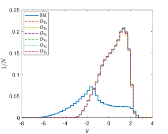
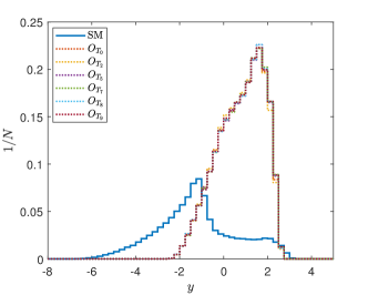
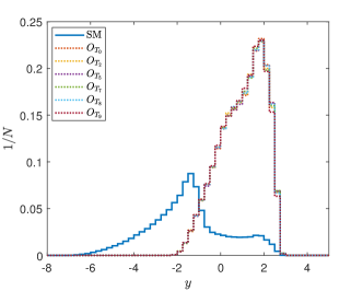
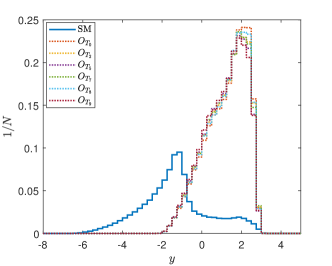
Figure 3: The normalized distributions of $y$ for the SM background and NP signals at different c.m. energies. The top-left panel corresponds to $\sqrt{s}=3\;{\rm TeV}$, the top-right panel corresponds to $\sqrt{s}=10\;{\rm TeV}$, the bottom-left panel corresponds to $\sqrt{s}=14\;{\rm TeV}$, and the bottom-right panel corresponds to $\sqrt{s}=30\;{\rm TeV}$.

After training, the $w^{j}$ and $b$ can be obtained, which are listed in Tables 5 and 6. In the following, to verify that there is no overfitting, we use validation datasets which use different events compared with the training data sets. The validation data sets consist of a data set with $600000$ events from the SM, and six data sets where each contains $100000$ events from one operator, i.e., the events from the $O_{T_{0,2,5,7,8,9}}$ operators. Denoting $y^{SM}$ and $y^{NP}$ as $y$ calculated with the SM training data set and the NP training data set. The normalized distributions of $y^{SM}$ and $y^{NP}$ are shown in Fig. 3. It can be seen in Fig. 3 that the distributions for $y^{SM}$ peak at $-1$ while the distributions for $y^{NP}$ peak at $+1$, indicating that $y$ can be used for discriminating the NP signals from the SM background. Besides, it can be seen that the larger the $\sqrt{s}$, the better the separation.

When the amount of data to be processed is very large, the operational efficiency of the event selection strategy is also a very important consideration. As can be seen from Table 5, some of the $w^{j}$ are much smaller than others. From the point of view of the space consisting of observables, this suggests that the best separation hyperplane is almost parallel to the axes corresponding to these observables. As a result, these observables play a relatively minor role in the event selection strategy. When computing power is an important factor, one can ignore these observables with very small $w$, i.e., only uses those observables with large $w$ to form a simplified event selection strategy. In this paper, we choose $w$ to form an event selection strategy that uses only $6$ observables, $\sum_{j=1,2,11,13,14,15}w^{j}({p_{i}^{j}-\bar{p}^{j}})/{d^{j}}+b>y_{th}^{s}$ (they are $E_{1},E_{2},{R_{13}},m_{12},m_{13},m_{23}$) and denote it as ‘simplified’ event selection strategy.

IV Expected constraints on the coefficients

$\sqrt{s}$	3 TeV	10 TeV	14 TeV	30 TeV
Unit of coefficient	$({\rm TeV}^{-4})$	$(10^{-3}\;{\rm TeV}^{-4})$	$(10^{-3}\;{\rm TeV}^{-4})$	$(10^{-4}\;{\rm TeV}^{-4})$
$f_{T_{0}}/\Lambda^{4}$	[$-0.3,0.3$]	[$-1.5,1.5$]	[$-0.5,0.5$]	[$-0.5,0.5$]
$f_{T_{2}}/\Lambda^{4}$	[$-0.5,0.5$]	[$-2.0,2.0$]	[$-0.8,0.8$]	[$-0.8,0.8$]
$f_{T_{5}}/\Lambda^{4}$	[$-0.06,0.06$]	[$-0.3,0.3$]	[$-0.1,0.1$]	[$-0.08,0.08$]
$f_{T_{7}}/\Lambda^{4}$	[$-0.1,0.1$]	[$-0.5,0.5$]	[$-0.15,0.15$]	[$-0.15,0.15$]
$f_{T_{8}}/\Lambda^{4}$	[$-0.01,0.01$]	[$-0.05,0.05$]	[$-0.015,0.015$]	[$-0.015,0.015$]
$f_{T_{9}}/\Lambda^{4}$	[$-0.016,0.016$]	[$-0.08,0.08$]	[$-0.02,0.02$]	[$-0.02,0.02$]

Table 7: The range of coefficients used in scanning.

When the NP signals cannot been found, the task is to set constraints on the operator coefficients. To estimate the expected constraints at the muon colliders, in this section, we generate events with the SM contribution, the NP contribution and the interference between the SM and the NP all included. The events are generated assuming one operator at a time, with the range of operator coefficients listed in Table 7.

It has been shown that $p_{T,\gamma}$ cut can effectively suppresses the SM backgrounds [75], in order to relieve the pressure on computing resources, in the standard cut we use $p_{T,\gamma}>0.1E_{\rm beam}$, where $E_{\rm beam}$ is the beam energy, and the other cuts w.r.t. the infrared divergence are as same as in Eq. 4.

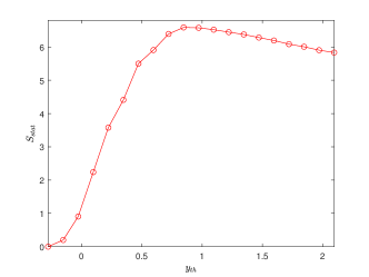
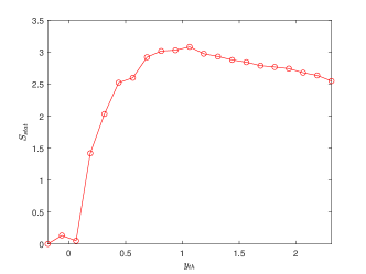
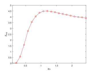
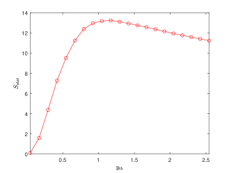
Figure 4: The signal significances as functions of $y_{th}$ for $O_{T_{0}}$ when the coefficients are picked as the upper bounds listed in Table 7, and the luminosities are picked as in the “conservative” case. The top-left panel corresponds to $\sqrt{s}=3\;{\rm TeV}$, the top-right panel corresponds to $\sqrt{s}=10\;{\rm TeV}$, the bottom-left panel corresponds to $\sqrt{s}=14\;{\rm TeV}$, and the bottom-right panel corresponds to $\sqrt{s}=30\;{\rm TeV}$.

$\sqrt{s}$	$3\;{\rm TeV}$	$10\;{\rm TeV}$	$14\;{\rm TeV}$	$30\;{\rm TeV}$
$y_{th}$	$1.221$	$1.063$	$1.201$	$1.170$

Table 8: The $y_{th}$ picked in this paper at $\sqrt{s}=3\;{\rm TeV}$, $10\;{\rm TeV}$, $14\;{\rm TeV}$, and $30\;{\rm TeV}$, respectively.

Using the event selection strategy optimized by the SVM is to cut off the events with $y<y_{th}$ where $y=w^{j}x^{j}+b$. In order to optimize the $y_{th}$, the cross-sections with $f_{T_{i}}$ equal to the upper bounds listed in Table 7 are considered. The statistical signal significance after cuts is calculated which is defined as [92, 93]

$$\begin{split}&\mathcal{S}_{stat}=\sqrt{2\left[(N_{\rm bg}+N_{s})\ln(1+N_{s}/N_{\rm bg})-N_{s}\right]},\end{split}$$ (5)

where $N_{s}=(\sigma-\sigma_{\rm SM})L$ and $N_{\rm bg}=\sigma_{\rm SM}L$, where $\sigma$ is the cross-section after cuts, $\sigma_{\rm SM}$ is the contribution of the SM after cuts, and $L$ representing the luminosity. In the “conservative” case [69], i.e., $L=1\;{\rm ab}^{-1}$, $10\;{\rm ab}^{-1}$, $10\;{\rm ab}^{-1}$ and $10\;{\rm ab}^{-1}$ at $\sqrt{s}=3\;{\rm TeV}$, $10\;{\rm TeV}$, $14\;{\rm TeV}$ and $30\;{\rm TeV}$, respectively, $\mathcal{S}_{stat}$ as functions of $y_{th}$ are calculated, and shown in Fig. 4. We choose $y_{th}$ which maximizes the $S_{stat}$, the results are listed in Table 8.

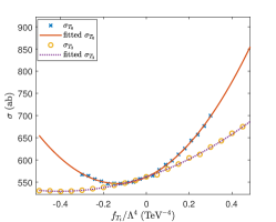
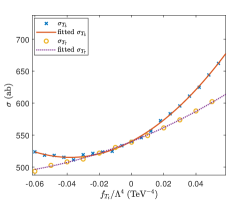
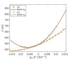
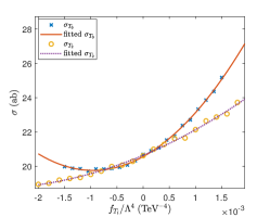
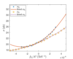
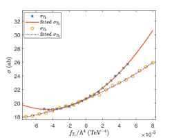
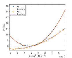
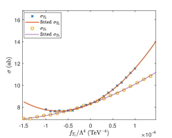
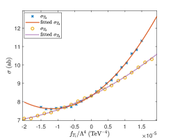
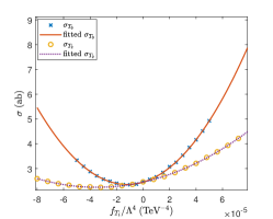
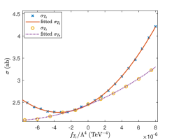
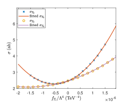
Figure 5: The cross-sections after cuts $\sigma$ compared with the fitted $\sigma$ according to bilinear functions of $f_{T_{i}}/\Lambda^{4}$ at different collision energies, $\sqrt{s}=3\;{\rm TeV}$ (row 1), $10\;{\rm TeV}(row2)$, $14\;{\rm TeV}$ (row 3), and $30\;{\rm TeV}$ (row 4).

After applying the event selection strategy, the total cross-section of the tri-photon process with aQGCs can be written as,

$$\begin{split}&\sigma=\sigma_{\rm SM}+\sigma_{\rm int}f_{T_{i}}/\Lambda^{4}+\sigma_{\rm NP}\left(f_{T_{i}}/\Lambda^{4}\right)^{2}.\end{split}$$ (6)

The results after cuts are shown in Fig. 5. It can be shown that the bilinear function fits well.

		3 TeV	10 TeV	14 TeV	30 TeV
	$S_{stat}$	$1\;{\rm ab}^{-1}$	$10\;{\rm ab}^{-1}$	$10\;{\rm ab}^{-1}$	$10\;{\rm ab}^{-1}$
		$(10^{-2}\;{\rm TeV^{-4}})$	$(10^{-4}\;{\rm TeV^{-4}})$	$(10^{-4}\;{\rm TeV^{-4}})$	$(10^{-5}\;{\rm TeV^{-4}})$
	2	[$-36.57,12.97$]	[$-29.58,10.95$]	[$-8.47,3.61$]	[$-5.34,2.95$]
$f_{T_{0}}(f_{T_{1}})/\Lambda^{4}$	3	[$-41.08,17.48$]	[$33.34,14.71$]	[$-9.68,4.81$]	[$-6.27,3.88$]
	5	[$-48.63,25.03$]	[$-39.65,21.01$]	[$-11.71,6.84$]	[$-7.84,5.45$]
	2	[$-91.62,20.67$]	[$-73.91,17.29$]	[$-20.29,5.91$]	[$-12.04,5.06$]
$f_{T_{2}}/\Lambda^{4}$	3	[$-99.70,28.77$]	[$-80.62,24.00$]	[$-22.50,8.12$]	[$-13.80,6.82$]
	5	[$113.71,42.78$]	[$-92.25,35.63$]	[$-26.31,11.93$]	[$-16.82,9.84$]
	2	[$-9.12,2.36$]	[$-7.46,1.98$]	[$-2.07,0.678$]	[$-1.25,0.568$]
$f_{T_{5}}(f_{T_{6}})/\Lambda^{4}$	3	[$-10.02,3.25$]	[$-8.21,2.73$]	[$-2.32,0.924$]	[$-1.44,0.760$]
	5	[$-11.55,4.79$]	[$-9.49,4.01$]	[$-2.74,1.34$]	[$-1.77,1.08$]
	2	[$-14.52,3.59$]	[$-5.34,2.97$]	[$-5.06,1.06$]	[$-2.86,0.939$]
$f_{T_{7}}/\Lambda^{4}$	3	[$-25.30,5.11$]	[$-19.09,4.21$]	[$-5.49,1.49$]	[$-3.21,1.29$]
	5	[$-28.02,7.83$]	[$-21.29,6.41$]	[$-6.25,2.24$]	[$-3.82,1.91$]
	2	[$-1.49,0.380$]	[$-1.18,0.312$]	[$-0.336,0.108$]	[$-0.200,0.0905$]
$f_{T_{8}}/\Lambda^{4}$	3	[$-1.64,0.525$]	[$-1.30,0.432$]	[$-0.376,0.147$]	[$-0.231,0.121$]
	5	[$-1.89,0.773$]	[$-1.50,0.635$]	[$-0.443,0.215$]	[$-0.284,0.174$]
	2	[$-0.897,0.572$]	[$-0.824,0.481$]	[$-0.883,0.171$]	[$-0.471,0.151$]
$f_{T_{9}}/\Lambda^{4}$	3	[$-4.05,0.814$]	[$-3.17,0.682$]	[$-0.953,0.242$]	[$-0.528,0.208$]
	5	[$-4.48,1.25$]	[$-3.53,1.04$]	[$-1.08,0.367$]	[$-0.628,0.308$]

Table 9: In the ”conservative” case, the projected sensitivities on the coefficients of the $O_{T_{i}}$ operators at the muon colliders for various c.m. energies and integrated luminosities.

		14 TeV	30 TeV
	$S_{stat}$	$20\;{\rm ab}^{-1}$	$90\;{\rm ab}^{-1}$
		$(10^{-5}\;{\rm TeV^{-4}})$	$(10^{-6}\;{\rm TeV^{-4}})$
	2	[$-76.61,27.93$]	[$-37.36,13.47$]
$f_{T_{0}}(f_{T_{1}})/\Lambda^{4}$	3	[$-86.31,37.63$]	[$-42.04,18.15$]
	5	[$-102.62,53.94$]	[$-49.91,26.02$]
	2	[$-188.35,44.59$]	[$-91.18,21.38$]
$f_{T_{2}}/\Lambda^{4}$	3	[$-205.71,61.96$]	[$-99.51,29.71$]
	5	[$-235.86,92.10$]	[$-113.94,44.14$]
	2	[$-19.13,5.15$]	[$-9.27,2.45$]
$f_{T_{5}}(f_{T_{6}})/\Lambda^{4}$	3	[$-21.07,7.10$]	[$-10.20,3.38$]
	5	[$-24.41,10.44$]	[$-11.79,4.97$]
	2	[$-13.41,7.83$]	[$-12.71,3.75$]
$f_{T_{7}}/\Lambda^{4}$	3	[$-51.14,11.39$]	[$-24.48,5.31$]
	5	[$-57.02,17.00$]	[$-27.28,8.11$]
	2	[$-3.10,0.819$]	[$-1.49,0.390$]
$f_{T_{8}}/\Lambda^{4}$	3	[$-3.41,1.13$]	[$-1.64,0.537$]
	5	[$-3.95,1.67$]	[$-1.89,0.791$]
	2	[$-1.95,1.26$]	[$-2.22,0.599$]
$f_{T_{9}}/\Lambda^{4}$	3	[$-8.92,1.80$]	[$-4.06,0.852$]
	5	[$-9.89,2.77$]	[$-4.51,1.30$]

Table 10: Same as Table 9 but for the “optimistic” case.

To estimate the expected constraints on the coefficients, both the luminosities in the “conservative” and “optimistic” cases are considered [69]. With the help of $\mathcal{S}_{stat}$ and the fitted cross-sections after cuts, the expected constraints on the operator coefficients at $2\sigma$, $3\sigma$, $5\sigma$ levels are calculated and presented in Table 9 and Table 10.

$\sqrt{s}$	$3\;{\rm TeV}$	$10\;{\rm TeV}$	$14\;{\rm TeV}$	$30\;{\rm TeV}$
$y_{th}$	$0.171$	$-0.087$	$0.326$	$0.095$

Table 11: Same as Table 8 but for the ‘simplified’ event selection strategy.

Figure 6: Same as Fig. 4 but for the ‘simplified’ event selection strategy.

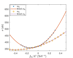
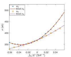
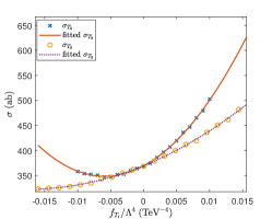
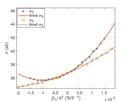
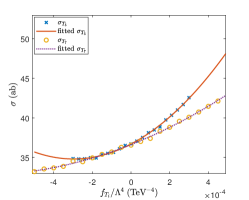
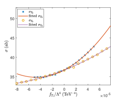
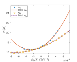
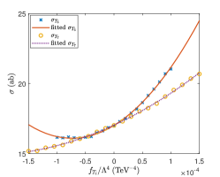
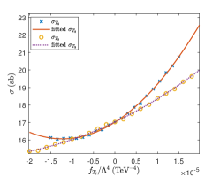
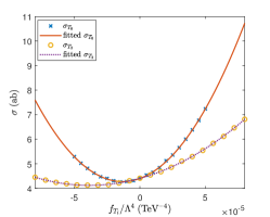
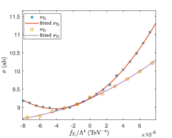
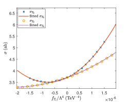
Figure 7: Same as Fig. 5 but for the ‘simplified’ event selection strategy.

		3 TeV	10 TeV	14 TeV	30 TeV
	$S_{stat}$	$1\;{\rm ab}^{-1}$	$10\;{\rm ab}^{-1}$	$10\;{\rm ab}^{-1}$	$10\;{\rm ab}^{-1}$
		$(10^{-2}\;{\rm TeV^{-4}})$	$(10^{-4}\;{\rm TeV^{-4}})$	$(10^{-4}\;{\rm TeV^{-4}})$	$(10^{-5}\;{\rm TeV^{-4}})$
	2	[$-39.43,13.80$]	[$-32.50,12.275$]	[$-9.23,3.89$]	[$-5.84,3.21$]
$f_{T_{0}}(f_{T_{1}})/\Lambda^{4}$	3	[$-44.23,18.61$]	[$-36.68,16.44$]	[$-10.52,5.18$]	[$-6.83,4.20$]
	5	[$-52.30,26.67$]	[$-43.64,23.41$]	[$-12.67,7.33$]	[$-8.50,5.87$]
	2	[$-99.92,22.20$]	[$-83.19,19.47$]	[$-21.31,6.38$]	[$-13.21,5.51$]
$f_{T_{2}}/\Lambda^{4}$	3	[$-108.61,30.89$]	[$-90.73,27.01$]	[$-23.66,8.73$]	[$-15.10,7.39$]
	5	[$123.68,45.96$]	[$-103.74,40.01$]	[$-27.66,12.73$]	[$-18.31,10.60$]
	2	[$-9.68,2.54$]	[$-8.16,2.22$]	[$-2.21,0.725$]	[$-1.36,0.614$]
$f_{T_{5}}(f_{T_{6}})/\Lambda^{4}$	3	[$-10.63,3.49$]	[$-8.99,3.05$]	[$-2.46,0.985$]	[$-1.57,0.819$]
	5	[$-12.27,5.13$]	[$-10.40,4.46$]	[$-2.91,1.43$]	[$-1.91,1.16$]
	2	[$-16.19,3.85$]	[$-6.64,3.32$]	[$-5.73,1.14$]	[$-3.15,1.02$]
$f_{T_{7}}/\Lambda^{4}$	3	[$-26.77,5.47$]	[$-20.66,4.70$]	[$-6.19,1.61$]	[$-3.52,1.39$]
	5	[$-29.66,8.36$]	[$-23.09,7.12$]	[$-7.00,2.42$]	[$-4.18,2.04$]
	2	[$-1.58,0.408$]	[$-1.30,0.356$]	[$-0.362,0.117$]	[$-0.220,0.0985$]
$f_{T_{8}}/\Lambda^{4}$	3	[$-1.73,0.562$]	[$-1.43,0.488$]	[$-0.404,0.159$]	[$-0.253,0.131$]
	5	[$-2.00,0.827$]	[$-1.65,0.714$]	[$-0.476,0.230$]	[$-0.309,0.187$]
	2	[$-0.970,0.613$]	[$-0.985,0.541$]	[$-0.889,0.182$]	[$-0.520,0.164$]
$f_{T_{9}}/\Lambda^{4}$	3	[$-4.32,0.872$]	[$-3.47,0.766$]	[$-0.962,0.256$]	[$-0.582,0.225$]
	5	[$-4.79,1.33$]	[$-3.87,1.16$]	[$-1.09,0.385$]	[$-0.687,0.331$]

Table 12: Same as Table 9, but for the ‘simplified’ event selection strategy.

		14 TeV	30 TeV
	$S_{stat}$	$20\;{\rm ab}^{-1}$	$90\;{\rm ab}^{-1}$
		$(10^{-5}\;{\rm TeV^{-4}})$	$(10^{-6}\;{\rm TeV^{-4}})$
	2	[$-83.58,30.13$]	[$-41.04,14.73$]
$f_{T_{0}}(f_{T_{1}})/\Lambda^{4}$	3	[$-93.99,40.53$]	[$-46.13,19.82$]
	5	[$-111.42,57.96$]	[$-54.64,28.33$]
	2	[$-197.60,48.32$]	[$-100.46,23.40$]
$f_{T_{2}}/\Lambda^{4}$	3	[$-216.12,66.85$]	[$109.52,32.46$]
	5	[$-248.01,98.74$]	[$-125.15,48.09$]
	2	[$-20.32,5.52$]	[$-10.13,2.66$]
$f_{T_{5}}(f_{T_{6}})/\Lambda^{4}$	3	[$-22.38,7.59$]	[$-11.14,3.67$]
	5	[$-25.91,11.11$]	[$-12.85,5.38$]
	2	[$-13.86,8.46$]	[$-14.38,4.06$]
$f_{T_{7}}/\Lambda^{4}$	3	[$-57.86,12.02$]	[$-27.09,5.77$]
	5	[$-64.20,18.36$]	[$-30.11,8.78$]
	2	[$-3.34,0.889$]	[$-1.64,0.427$]
$f_{T_{8}}/\Lambda^{4}$	3	[$-3.67,1.22$]	[$-1.80,0.587$]
	5	[$-4.24,1.79$]	[$-2.08,0.863$]
	2	[$-2.31,1.33$]	[$-2.50,0.654$]
$f_{T_{9}}/\Lambda^{4}$	3	[$-8.98,1.92$]	[$-4.49,0.928$]
	5	[$-9.98,2.92$]	[$-4.98,1.41$]

Table 13: Same as Table 12, but for the “optimistic” case.

In the ‘simplified’ event selection strategy case, the $S_{state}$ as the function of $y_{th}$ are also calculated and presented in Fig. 6. The $y_{th}$ in the ‘simplified’ event selection strategy case are listed in Table 11. After the $y_{th}$ are chosen, the fitted cross-sections after cuts are shown in Fig. 7. Similarly, the expected constraints for both the “conservative” and “optimistic” cases are calculated, they are presented in the Tables 12 and  13. Comparing these constraints with those in Table 9 and Table 10, we observe that the values of the constraints in the ‘simplified’ case are very similar. This indicates that the ‘simplified’ event selection strategy is also efficient.

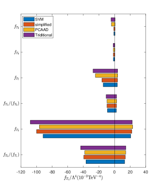
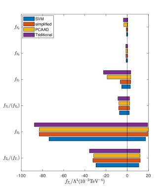
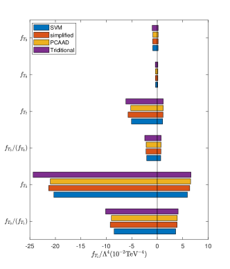
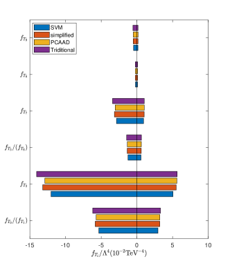
Figure 8: Comparison of the expected coefficient constraints obtained by different algorithms. The top-left panel corresponds to $\sqrt{s}=3\;{\rm TeV}$, the top-right panel corresponds to $\sqrt{s}=10\;{\rm TeV}$, the bottom-left panel corresponds to $\sqrt{s}=14\;{\rm TeV}$, and the bottom-right panel corresponds to $\sqrt{s}=30\;{\rm TeV}$.

This paper employs the same energies and luminosities as those in Refs [75, 56], but with a different event selection strategy. To estimate the effectiveness of our approach, we compare the expected coefficient constraints in this paper with those in Refs. [75, 56], the results are shown in Fig. 8, which clearly demonstrates the bounds in this paper are tighter than those in Refs. [75, 56]. Note that, Ref. [75] uses traditional event selection strategy, and Ref. [56] uses a ML event selection strategy. It can also be shown that, the ‘simplified’ event selection strategy has compatible efficiency. Therefore, we can conclude that the SVM algorithm proves to be a useful and efficient tool to optimize the event selection strategy to search for the signals from NP.

V Summary

The search for NP signals involves the analyzing of a large amount of experimental data, and therefore the efficiency becomes a very important consideration in the phenomenological study and in the experiments. Both the ML algorithms and quantum computers offer the potential in accelerate the relevant calculations. In this paper, we consider a procedure to use the SVM to optimize an event selection strategy to study the signals from the NP. The SVM is a ML algorithm which can be accelerated using quantum computing, and is expected to be able to distinguish the signal events from the background. In this paper, we focus on the tri-photon process which is sensitive to the dimension-8 operators contributing to the aQGCs.

The procedure to use the SVM to obtain an optimized event selection strategy is proposed in this paper. With the help of the optimized event selection strategy and the ‘simplified’ event selection strategy, the expected constraints on the operator coefficients are calculated. The results demonstrate the effectiveness of the SVM in the searching of NP signals.

The SVM has already been proved to be compatible with the quantum computers. In the future, we expect that SVM will serve as a bridge between the quantum computing and the phenomenological study of the NP and the HEP experiments, enabling more efficient discovery of the NP.