Universal relations in compact stars with exotic degrees of freedom

Abstract

The nature of the highly dense matter inside the supernova remnant compact star is not constrained by terrestrial experiment and hence is modeled phenomenologically to accommodate the astrophysical observations from compact stars as the observable properties of the compact stars are highly sensitive to the microscopic model of highly dense matter. However, there exists some universal relations between some macroscopic properties of compact stars independent of the matter model. We examine the universal relations for quantities moment of inertia - tidal love number - quadrupole moment. We also study some already established universal relations in non-radial oscillation frequencies with star compactness for the baryonic star with core composed of heavier baryons and for the hybrid star with core composed of strange quark matter in CFL phase surrounded by nucleonic matter. We find the hybrid star with core of quark matter in the CFL phase obeys the same universal relation as the hybrid star with normal quark matter. However, the baryonic star with strange and non-strange heavier baryons at the inner core fails to satisfy the universal relations.

1 Introduction

The massive stars end their lives by core collapse supernova explosion leaving highly compact stars (CS) as central objects. The CSs have an average density $\sim 10^{14}$ gm/cm³. The average density of matter inside such a compact object is several times the normal nuclear saturation density ($n_{0}$). These compact objects accommodate the extremely dense matter in the universe and thus allow insights into various new aspects of dense matter physics. Such high densities are not attainable in any laboratory or terrestrial experiments and hence the exact composition of matter as well as the inter-particle interaction inside the compact objects is unknown. The so-called equation of state (EOS), which describes the relationship between energy density ($\epsilon$) and pressure (p), at extremely high densities, is among the most uncertain aspects of nuclear physics. Consequently, many phenomenological models are discussed with different compositions and different inter-particle interactions. These extremely compact stars have an interior structure that is highly sensitive to their EOS. Consequently, these factors dictate the external characteristics of the objects in question, including their mass and radius; their deformability, as indicated by their quadrupole moment and tidal Love number; and their rotation rate, which is defined by their moment of inertia. The macroscopic properties of CSs are highly sensible to the microscopic properties of highly dense matter which are still unknown and model-dependent as of now. Hence, the only way to minimize the theoretical uncertainties regarding highly dense matter is to fit the proposed models with the astrophysical observations coming from these CSs.

However, Yagi and Yunes in 2013 discoveredthat some combination of physical parameters doesn’t depend on the EOS and follows universal relations [1, 2] They showed that the relations between moment of inertia (I), tidal Love number (L) and quadrupole moment (Q) of CSs are independent of EOS of highly dense matter - irrespective of whether the matter is pure nucleonic or deconfined strange quark matter. The above-mentioned variables obey a universal relation. There are several quasi-normal modes like the fundamental f-mode, pressure p-modes, gravity g-modes, spacetime w-mode, etc [3, 4, 5], each classified based on the restoring forces which work bring the star to equilibrium. For example, the f- and p- modes, which are acoustic waves in the star, are restored by fluid pressure while g-modes which arise due to density discontinuities or temperature and composition variations are restored by gravity (buoyancy). In this work, we adopt the Cowling classification, where the various modes are separated by the number of radial nodes [6, 7]. The f-mode, whose frequency lies between those of the p- and g-modes, has no radial node number, while g- and p- modes can have an arbitrary number of radial nodes greater than 0. For the same radial node number, p-modes have a higher frequency than g-modes. Several of these modes can be excited during supernovae explosions or in an isolated perturbed compact star as in the post-merger phase of binary compact stars [8, 9, 10]. Even during the inspiral phase of compact stars, the f-mode may be excited [11, 12]. Quadrupolar oscillations (l=2) of all modes lead to the emission of GWs. With the advent of enhanced next-generation telescopes like the Cosmic Explorer and the Einstein telescope which carry about 10 times the sensitivity of Advanced LIGO, the possibility of detection of these modes increase [8]. Various previous works have explored non-radial modes in cold and finite temperature neutron stars [13, 14, 15, 16]. Although the high-frequency p-modes aren’t expected to be detected by the next-generation GW detectors, we include their study for the sake of completeness. Some years ago, Andersson and Kokkotas [17] proposed an empirical relation for the f-mode oscillation frequency $\omega$, based on Newtonian theory of stellar perturbations. They observed that in full GR, $\omega$ depends almost linearly on the square root of the average density. Another relation, based on estimates using the quadrupole formula, was established for the damping time due to gravitational wave emission, $\tau$. Later, Benhar et al. [18] presented further results that included more and newer equations of state, updating the fits from [17]. The average frequencies $\omega$ were systematically lower than the one for the old EOS sample, which they attributed to the fact that the new sample included stiffer EOSs. The paper that thoroughly studied the universality is [19]. They considered a wide range of masses and the EOSs to minimize the uncertainty. In our work, we took it further and computed the universality for CSs.

Universal relations are crucial because they enable us to calculate the others if we know one parameter. When it comes to CSs, it is possible to compute the love number and Q without physically measuring them if I can be measured in some way. This is extremely useful, as both are challenging to quantify for binaries separated by a significant distance. By accurately measuring the love number in coalescing binaries, it is possible to infer the Q and, consequently, gain insight into the spins of the coalescing binary CSs. Recently, universal relations have been getting some attention [20, 21, 22, 23, 24, 25, 26, 27, 28, 29, 30, 31, 32, 33, 34, 35, 36, 37, 38, 39, 40]. The first study of the I-Q relation for rapidly rotating NSs was done by Doneva [41]. They found that the I-Q relation is broken and becomes more EOS-dependent for NSs with a fixed frequency. However, it was soon found by Pappas & Apostolatos [42], and Chakrabarti et al. [31] that the I-Q relation can remain approximately EOS-insensitive if one chooses suitable dimensionless parameters instead of dimensional quantities.

The most studied and discussed possibility of matter at such high density is pure nucleonic matter - the matter composed of mostly neutrons with some admixture of protons and electrons. However, the appearance of exotic degrees of freedom in the interior of massive NSs where the density is a few times $n_{0}$ tends to be feasible, although it remains an open question. For example, there are possibilities of the appearance of strange baryons [43, 44, 45, 46, 47, 48], non-strange heavier baryons [49, 50, 51, 52, 53, 54, 55], Boson condensates [56, 57, 58, 59, 60, 61] etc. Another possibility is the existence of strange quark matter (SQM) inside the stars [62, 63, 64]. At that much high density, the baryons, may get decomposed into their constituent quarks and generate a region of deconfined SQM [65, 66]. This leads to birth of hybrid star (HS) composed of SQM at the core surrounded by baryonic matter up to surface [67, 68, 21, 69, 70, 71]. Moreover, at high enough density ($\mu>>T$), there may exist the Color-Flavor-Locked (CFL phase), which is a superconducting phase of SQM [72, 73, 74]. Most of the studies regarding universal relations have been carried out with neutron stars composed of pure nucleonic matter. Recently, the universality of HS in various temporal and rotational conditions has been studied in refs [21, 39]. The implication of GW170817 with universal relations for HS has been studied in ref. [21] considering maxwell construction and universal relation for hot and cold rapidly rotating HS has been considered in ref. [39].In recent works we extend the study of universilities in the case of CS with strange and heavier non-strange baryons as well as SQM in Color-Flavor-Locked (CFL) phase inside the interior of the star.

In the next section (sec 2, we describe properties of matter with exotic degrees of freedom and the structure of CS with those kind of matter in the inner core. In sec, 3, we discuss the non-radial modes and determine their frequencies of CS with heavier baryons and SQM in CFL phase inside the core. Next, in sec. 4 we study the universal relations between different quantities.

2 Star structure with exotic degrees of freedom

In this work, we study the universal relation for different quantities related to CS with heavier baryons and SQM in the CFL phase in the core of the star. In this context, first, we briefly discuss the star with the core of heavier baryons.

2.1 Baryonic star

Inside CS, near the surface, the matter is purely nucleonic. With the increase in density towards the center, other heavier baryons may appear. To describe the EOS of this matter we consider density-dependent parametrization within the Covariant Density Functional (CDF) model. The interaction between nucleons is mediated by the exchange of isoscalar-scalar $\sigma$, isoscalar-vector $\omega$, and isovector-vector $\rho$ mesons. In order to account for the hyperonic interactions, in addition to the mesons mentioned before another hidden strangeness isoscalar-vector $\phi$-meson is taken into consideration. In this work, we have considered the constituent particles as a baryonic octet ($b$) along with $\Delta$-resonances in the baryonic sector following ref.-[55]. In the density-dependent coupling scenario, in order to maintain thermodynamic consistency, we have to take into account a re-arrangement term as,

$$\Sigma^{r} =\sum_{b}\left[\frac{\partial g_{\omega b}}{\partial n}\omega_{0}n_{b}-\frac{\partial g_{\sigma b}}{\partial n}\sigma n_{b}^{s}+\frac{\partial g_{\rho b}}{\partial n}\rho_{03}\bm{\tau}_{b3}n_{b}+\frac{\partial g_{\phi b}}{\partial n}\phi_{0}n_{b}\right]+\sum_{\Delta}(\psi_{b}\longrightarrow\psi_{\Delta}^{\nu}),$$ (1)

where $n^{s}=\langle\bar{\psi}\psi\rangle$ and $n=\langle\bar{\psi}\gamma^{0}\psi\rangle$ denoting the scalar and vector (number) densities respectively. Here, $g_{\chi b}$ represents the density-dependent coupling with $\chi=\omega,~{}\sigma,~{}\rho,~{}\phi$. Additionally $\psi_{b},~{}\psi_{\Delta}^{\nu}$ represent Dirac-fields of the baryon-octet and Schwinger-Rarita fields of $\Delta$-quartet respectively.

For the meson-heavier baryon coupling parameters, we have considered them to be on the density-dependent footing as well. SU(6) symmetry and quark counting rule are implemented to account for the vector couplings [75]. In the case of scalar meson-hyperon couplings, we consider the following optical potential depths: $U_{\Lambda}^{(N)}(n_{0})=-30$ MeV [76], $U_{\Sigma}^{(N)}(n_{0})=+30$ MeV [77] and $U_{\Xi}^{(N)}(n_{0})=-18$ MeV [78]. For a recent overview on meson-hyperon couplings, the readers may refer to ref.-[79]. Because of the scarce information on $\Delta$-nucleon interactions, we treat the meson-$\Delta$ couplings as parameters. In this work, we consider the coupling values as $g_{\sigma\Delta}=1.2g_{\sigma N}$, $g_{\omega\Delta}=1.1g_{\omega N}$ and $g_{\rho\Delta}=g_{\rho N}$. $\Delta$-baryons being non-strange in nature do not couple with $\phi$-meson (i.e. $g_{\phi\Delta}=0$). The readers may refer to ref.-[80] to know further about the recent development regarding $\Delta$-potential in dense matter.

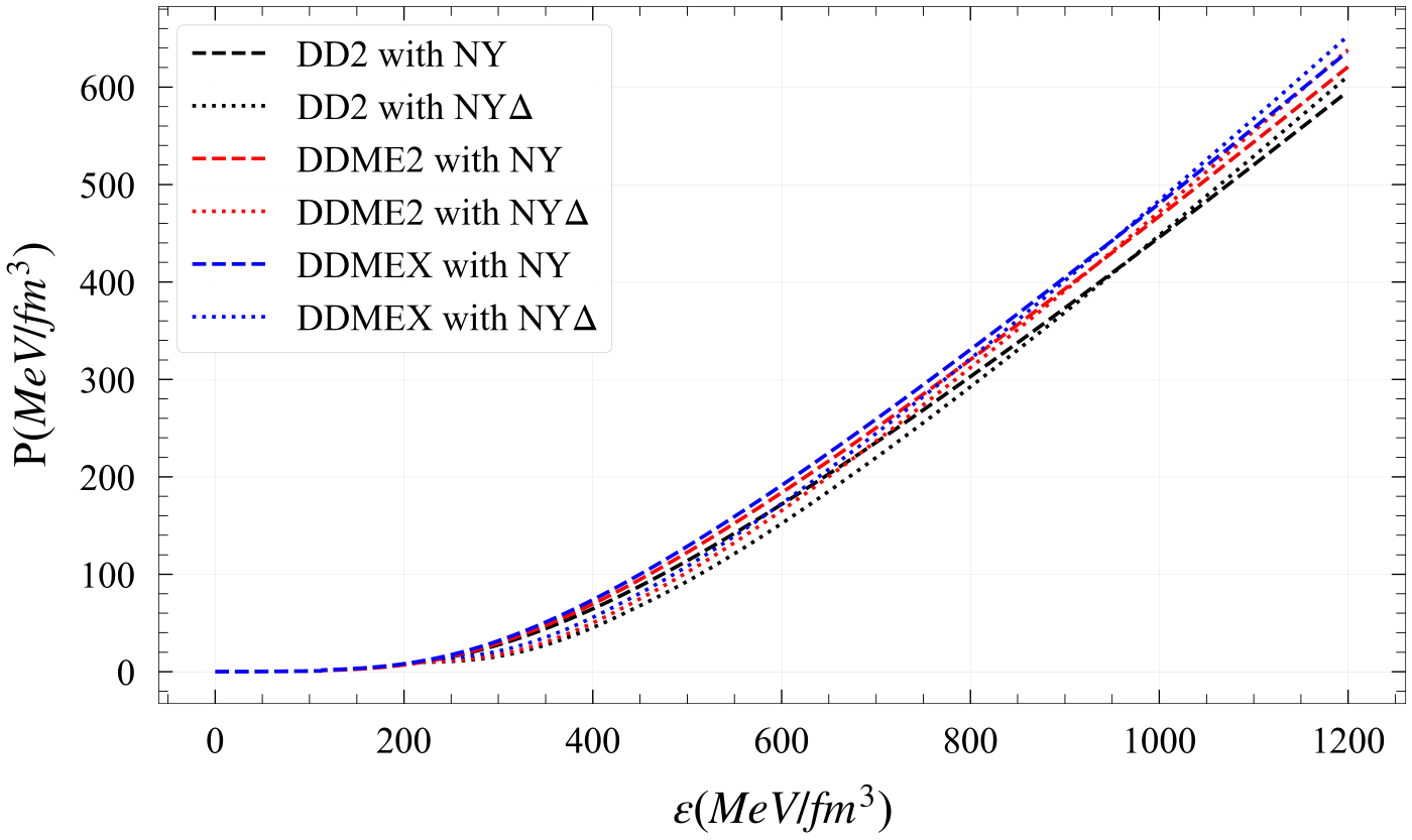
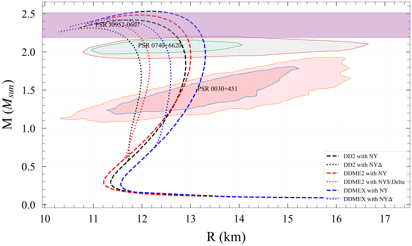
Figure 1: The variation of pressure with energy density and the corresponding mass-radius relations

Appearance of strange baryons makes EOS softer as shown in Fig. 1. EOS becomes, even more, softer after including $\Delta$ baryons. Still, all the M-R curves satisfy the M-R constraints. Here, we apply M-R constraints of PSR J0952-0607, PSR J0030+451, and PSR J0740+6620 as given in references [81], [82] and [83] respectively.

2.2 Hybrid star

With the increase in density towards the center, the quarks may get deconfined and form SQM at the core of the star, which is an HS. We consider here HS with deconfined SQM at the core surrounded by pure nucleonic matter. For quark matter, we consider two possibilite: one is superconducting quark matter in CFL phase and the other is without CFL phase, normal SQM matter. For the CFL phase, we use the MIT bag model including the gap term as mentioned in ref. [84, 85, 86]. Normal SQM is modeled with vector bag model (vBAG) [64, 87, 88] and MIT bag model with some interacting terms as mentioned in ref. [89, 66].

2.2.1 Superconducting quark matter

In this phase, quarks are paired up in such a way that they form color-neutral and flavor-neutral condensates, and this leads to a unique and stable ground state of matter. In such a scenario, these paired quarks would move together with correlated momentum, somewhat analogous to Cooper pairs in superconductors. Studying the CFL phase in neutron stars is intimately linked to quantum chromodynamics (QCD), the theory of strong interactions. Understanding the behavior of matter under extreme conditions is an essential aspect of fundamental physics, and it can provide insights into the behavior of quarks and gluons under extreme pressures and densities. Here, each quark has a common Fermi momentum ($\nu$) and number density ($n$) to form Cooper pairs

$$\nu=2\mu-\sqrt{\mu^{2}+\frac{{m_{s}}^{2}}{3}}$$ (2)

$$n=\frac{\nu^{3}+2\Delta^{2}\mu}{\pi^{2}}$$ (3)

In these equations, CFL energy gap term is denoted by $\Delta$, and quark number chemical potential is $\mu=(\mu_{u}+\mu_{d}+\mu_{s})/3$. The thermodynamic potential of this phase is given by

$$\Omega_{CFL}=\Omega_{free}-\frac{3}{\pi^{2}}\Delta^{2}\mu^{2}+B$$ (4)

Here, $B$ is the bag parameter. $\Omega_{free}$ can be given as

$$\Omega_{free}=\frac{6}{\pi^{2}}\int_{0}^{\nu}(p-\mu)p^{2}dp+\frac{3}{\pi^{2}}\int_{0}^{\nu}(\sqrt{p^{2}+{m_{s}}^{2}}-\mu)p^{2}dp$$ (5)

The pressure ($P$), and energy density ($\epsilon$) of CFL phase are

$$P=-\Omega_{CFL}$$ (6)

$$\epsilon=\sum_{i=u,d,s}\mu_{i}n_{i}+\Omega_{CFL}$$ (7)

2.2.2 Normal quark matter

The original MIT bag model considered quarks to be confined inside a bag, and these quarks can freely move inside this bag [90, 91]. Frahi and Jaffe have introduced the QCD interactions at small distances with $O(\alpha_{s})$ correction [89]. We will consider it as the MIT bag model.
(i) MIT bag model
The thermodynamic potential for SQM with the MIT bag model is given by

$$\begin{split}\Omega_{q}&=-\frac{1}{4\pi^{2}}\Biggl{\{}\mu_{q}\sqrt{\mu_{q}^{2}-m_{q}^{2}}\left(\mu_{q}^{2}-\frac{5}{2}m_{q}^{2}\right)+\frac{3}{2}m_{q}^{4}\ln{\frac{\mu_{q}+\sqrt{\mu_{q}^{2}-m_{q}^{2}}}{m_{q}}}\\ &-\frac{2\alpha_{s}}{\pi}\Biggl{[}3\left(\mu_{q}\sqrt{\mu_{q}^{2}-m_{q}^{2}}-m_{q}^{2}\ln{\frac{\mu_{q}+\sqrt{\mu_{q}^{2}-m_{q}^{2}}}{m_{q}}}\right)^{2}\\ &-2\left(\mu_{q}^{2}-m_{q}^{2}\right)^{2}-3m_{q}^{4}\ln^{2}{\frac{m_{q}}{\mu_{q}}}\\ &+6\ln{\frac{\sigma}{\mu_{q}}}\left(\mu_{q}m_{q}^{2}\sqrt{\mu_{q}^{2}-m_{q}^{2}}-m_{q}^{4}\ln{\frac{\mu_{q}+\sqrt{\mu_{q}^{2}-m_{q}^{2}}}{m_{q}}}\right)\Biggr{]}\Biggr{\}}\end{split}$$ (8)

where $\mu_{q}$ and $m_{q}$ denote the chemical potential and mass of each quark q and $\sigma$ is the renormalization scale. The number density of each flavor can be given by the following equation

$$n_{q}=-\frac{\partial\Omega_{q}}{\partial\mu_{q}}$$ (9)

The thermodynamic potential of the electron is

$$\Omega_{e}=-\frac{\mu_{e}^{4}}{12\pi^{2}}$$ (10)

and EOS can be obtained through the relations

$$\epsilon=\sum_{q=u,d,s}(\mu_{q}n_{q}+\Omega_{q})+\Omega_{e}+B$$ (11)

$$P=-\sum_{q=u,d,s}\Omega_{q}-\Omega_{e}-B$$ (12)

(ii) vBAG model
The Lagrangian density of SQM with the vBAG model is given by the following equation as

$${\cal L}_{Q} =\sum_{q=u,d,s}\left[\bar{\psi}_{q}\{\gamma_{\mu}\left(i\partial^{\mu}-g_{qV}V_{\mu}\right)-m_{q}\}\psi_{q}-B\right]\Theta(\bar{\psi}_{q}\psi_{q})$$ (13)

$$-\frac{1}{4}{\left(\partial_{\mu}V_{\nu}-\partial_{\nu}V_{\mu}\right)}^{2}+\frac{1}{2}{m^{2}_{V}}{V_{\mu}}V^{\mu}+\bar{\psi}_{e}\left(\gamma_{\mu}i\partial^{\mu}-m_{e}\right)\psi_{e}$$

where $\psi_{q}$ is the field of quark q considering it as a fermion and $m_{q}$ is its mass. Similarly, $V_{\mu}$ and $m_{V}$ are the field of the mediator and its mass respectively. $B$ denotes the famous bag parameter and $\Theta$ is the heavy side function that is unity inside the bag and zero outside the bag. After solving equations of motions for the Lagrangian density, the chemical potential gets shifted as

$$\mu_{q}=\sqrt{(k_{fq})^{2}+(m_{q})^{2}}+g_{qV}V_{0}$$ (14)

The energy density of SQM matter within the vBAG model is

$$\epsilon =\frac{3}{\pi^{2}}\sum_{q}\int_{0}^{k_{f_{q}}}\left(\sqrt{(k)^{2}+(m_{q})^{2}}+g_{qV}V_{0}\right)k^{2}dk$$ (15)

$$-\frac{1}{2}\left({m_{V}}{V_{0}}\right)^{2}+B,$$

here $V_{0}$ is the mean value of $V_{\mu}$ in ground state. From energy density, pressure can be obtained by the following equation

$$P=\sum_{q}\mu_{q}n_{q}-\epsilon$$ (16)

where $n_{q}$ signifies number density of quark $q$.

2.2.3 Mixed phase

When we establish equilibrium between the baryonic phase and quark phase there exists a mixed phase region. In this region, global charge neutrality is maintained rather than local charge neutrality as

$$\chi\rho_{c}^{Q}+(1-\chi)\rho_{c}^{B}=0,$$ (17)

where $\chi$ is the volume fraction of quark matter with respect to baryonic matter and $\rho_{c}$ is the charge density. Superscripts B and Q denote the baryonic phase and quark phase respectively. The energy density of mixed-phase (MP) is given by the following equation

$$\epsilon_{MP}=\chi\epsilon_{Q}+(1-\chi)\epsilon_{B}$$ (18)

here $\epsilon_{Q}$ and $\epsilon_{H}$ are the energy densities of quark matter and baryonic matter respectively. The baryonic density of matter in the mixed phase is

$$\rho_{MP}=\chi\rho_{Q}+(1-\chi)\rho_{B}$$ (19)

Baryonic matter density for quark matter is $\rho_{Q}=(n_{u}+n_{d}+n_{s})/3$. The pressure of mixed-phase is equal to the pressure of quark matter and baryonic matter.

2.3 Matter and star properties for different matter EOSs

To study the universal relations between different quantities of the star obtained from different EOSs of HS, we consider different density-dependent parametrizations for baryonic matter. For quark matter, we consider both the superconducting phase and normal quark matter with different types of interactions. To construct HS we choose different combinations of them which are tabulated in table 1

B.M.	Q.M.	$B^{1/4}$
		(MeV)
DD2	CFL	190	$\Delta=30$ (MeV)
DDMEX	CFL	205	$\Delta=15$ (MeV)
DDME2	CFL	205	$\Delta=30$ (MeV)
DD	vBAG	180	$G_{V}=0.25$ ($fm^{2}$)
DD	vBAGs	172	$G_{V}=0.17$ ($fm^{2}$)
DD	MITbag	160	$\alpha_{s}=0.8$
DD	MITbags	174	$\alpha_{s}=0.3$

Table 1: Set of parameters we used for HSs EOS, B.M. denotes baryonic matter and Q.M. denotes quark matter

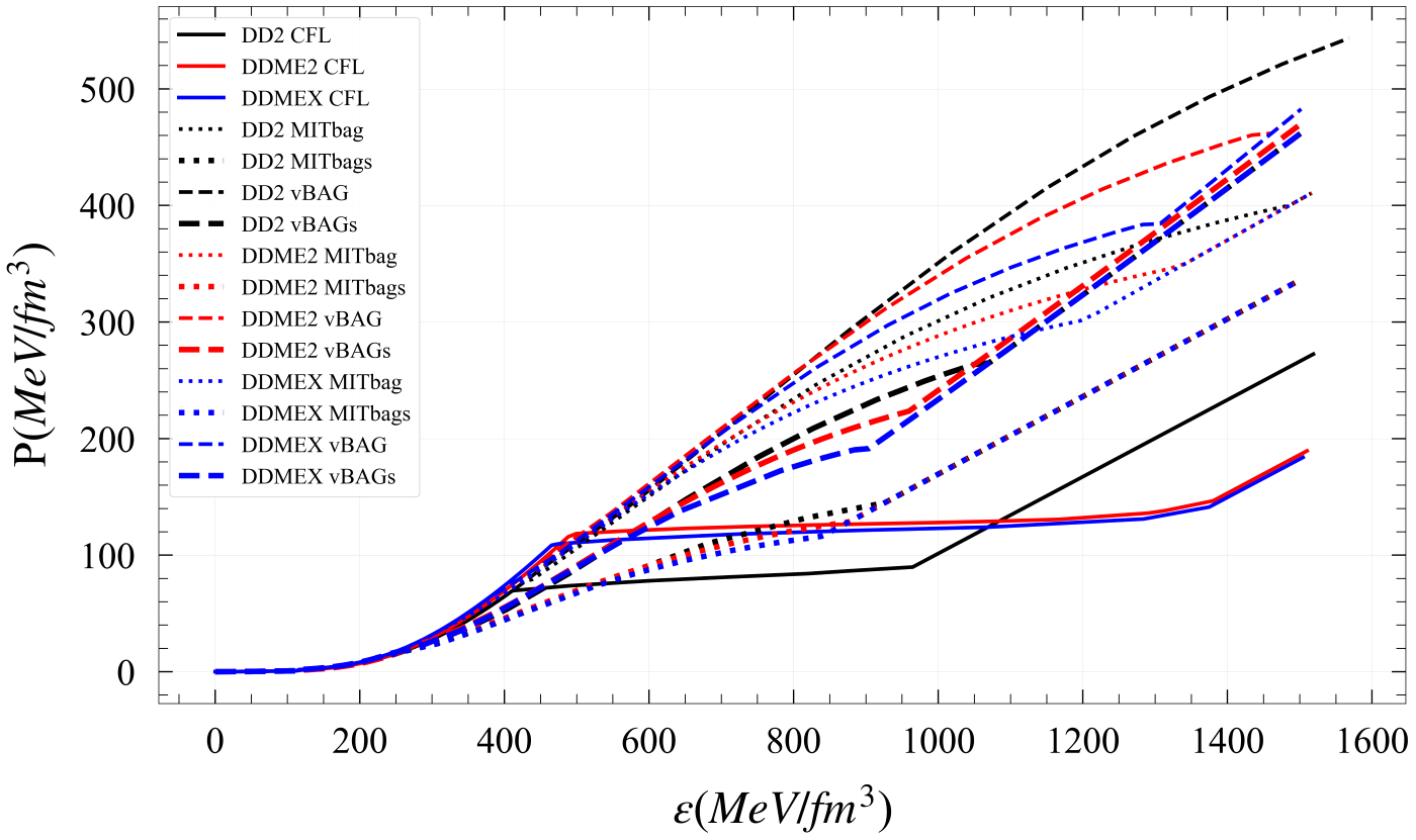
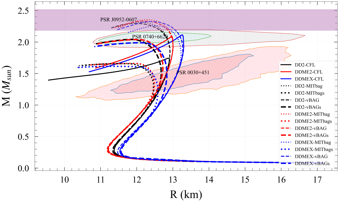
Figure 2: The variation of pressure with energy density and the corresponding mass-radius relations

We represent the EOS of matter in Fig. 2. Due to the presence of repulsive vector interactions, the EOS of quark matter becomes very stiff with the vBAG model as discussed [71]. On the other hand, there is no such repulsive interaction in the CFL phase that outcomes softer quark matter. With the CFL phase, the onset density of phase transition is very sensitive to the bag parameter ($B$) but not that sensitive to the gap parameter ($\Delta$). Similarly, for vector bag model, the width of the mixed-phase region is very susceptible to coupling parameters ($G_{V}$). The property of EOS of quark matter with the MIT bag model mainly depends on the strong coupling constant ($\alpha_{s}$).

After constructing the EOS, we solve the Tolman-Oppenheimer-Volkoff (TOV) equations to obtain the mass-radius (M-R) relations for non-rotating stars, which are shown in Fig. 2 along with recent observational constraints.

As quark matter appears at higher density inside the core, the maximum mass of the star is contingent on the properties of quark matter EOS. Due to the soft nature of CFL phase EOS, the appearance of the quark matter phase in the core of the star creates an unstable region in the M-R graph (decrease of the star’s mass with its increasing central energy density). However, there exists a very small stable M-R region near the maximum mass with the mixed phase at the center of the star. So, we could not conclude about the presence of quark matter in the CFL phase with these M-R constraints. We consider the parameters for all EOS models to satisfy all the M-R constraints of all three pulsars PSR J0952-0607, PSR J0030+451, and PSR J0740+6620.

3 Non Radial Modes

3.1 Relativistic Cowling Approximation

Since the non-radial oscillation formalism is developed in linearised gravity, the line element of a non-rotating neutron star is taken as:

$$ds^{2}=-e^{2\Phi(r)}dt^{2}+e^{2\Lambda(r)}dr^{2}+r^{2}d\theta^{2}+r^{2}\sin^{2}{\theta}d\phi^{2}$$ (20)

The fluid Lagrangian displacement vector is assumed to be: [92]

$$\xi^{i}=\left(e^{-\Lambda}W,-V\partial_{\theta},-V\sin^{-2}\theta\partial_{\phi}\right)r^{-2}\mathcal{Y}_{lm}(\theta,\phi)$$ (21)

where $\mathcal{Y}_{lm}(\theta,\phi)$ are the spherical harmonics. $W$ and $V$ are perturbative fluid variables, which are functions of $r$ with a harmonic time dependence $W(t,r)=W(r)e^{i{\omega}t}$ and $V(t,r)=V(r)e^{i{\omega}t}$. The mode frequencies ($\omega$) are thus found by solving the following system of ordinary differential equations [92]:

$$W^{\prime} =\derivative{\epsilon}{p}\left[{\omega}^{2}r^{2}e^{\Lambda-2\Phi}V+\Phi^{\prime}W\right]-l(l+1)e^{\Lambda}V$$ (22)

$$V^{\prime} =2\Phi^{\prime}V-r^{-2}e^{\Lambda}W$$

where $\epsilon$ is the energy density and $p$ the pressure. The dash (^′) represents a derivative with respect to the radius. The boundary conditions at the center of the star are $W(r\to 0)=Ar^{l+1}$ and $V(r\to 0)=-Ar^{l}/l$, where $A$ is an arbitrary constant, usually taken to be $1$.

The surface boundary condition corresponds to the fluid pressure vanishing at the surface of the star ($r=R$):

$${\omega}^{2}e^{\Lambda(R)-2\Phi(R)}V(R)+\frac{1}{R^{2}}\frac{d\Phi(r)}{dr}\bigg{|}_{r=R}W(R)=0$$ (23)

To solve these equations, we first solve the stellar structure equations for a particular central energy density, to get all the metric coefficients as functions of $r$. These coefficients are then used while solving the oscillation mode equations (eq. 22). Since we need to find $\omega$, we use the shooting method: first, a guess value of $\omega$ is used to solve the mode oscillation equations, after which we check if the surface boundary condition (eq. 23) is satisfied. If not, the guess is improved via the Newton-Raphson iteration scheme. The lowest frequency solution to the oscillation mode equation has no radial node and thus corresponds to the f-mode frequency. The next highest solution has one radial node and is thus the first p-mode (p1-mode). Although [7] suggests that this classification fails before 0.4 seconds of the bounce, for the models in consideration in this work, the Cowling classification holds good. The number of radial nodes was found by counting the number of times the perturbative variables $W$ and $V$ become $0$ within $r<R$ since this condition ensures that the three-velocity of the fluid (which is the time derivative of the fluid Lagrangian displacement vector), becomes $0$ at those points. The correctness of our code was ensured when our results matched with those reported in [13, 16].

3.2 Fully general relativistic Calculations

The equations that need to be solved and the various techniques required to solve them have been examined in great detail in several previous works [4, 5, 93, 94, 95, 14] and we simply state them for completeness.

In this work, we follow the method of direct numerical integration, first proposed by [4, 5] and refined by [96]. The perturbed metric is taken as:

$$ds^{2} =-e^{2\Phi(r)}(1+r^{l}H_{0}(r)\mathcal{Y}_{lm}e^{i\omega t})dt^{2}-2i\omega r^{l+1}H_{1}(r)\mathcal{Y}_{lm}e^{i\omega t}dtdr$$

$$+e^{2\Lambda(r)}(1-r^{l}H_{0}(r)\mathcal{Y}_{lm}e^{i\omega t})dr^{2}+r^{2}(1-r^{l}K(r)\mathcal{Y}_{lm}e^{i\omega t})(d\theta^{2}+\sin^{2}\theta\ d\phi^{2})$$ (24)

while the fluid displacement vector in terms of the perturbation functions $W(r)$ and $V(r)$ is:

$$\xi^{i}=\left(r^{l-1}e^{-\Lambda}W(r),-r^{l-2}V(r)\partial_{\theta},-r^{l-2}\sin^{-2}\theta V(r)\partial_{\phi}\right)\mathcal{Y}_{lm}(\theta,\phi)e^{i\omega t}$$ (25)

Lindblom and Detweiller [4, 5] introduced a new function $X(r)$ to replace $V(r)$ and the relations between all these functions are as follows:

$$H_{0} =\left\{8\pi r^{3}e^{-\Phi}X-\quantity[\frac{1}{2}l(l+1)(m+4\pi r^{3}p)-\omega^{2}r^{3}e^{-2(\Lambda+\Phi)}]H_{1}\right.$$

$$\left.+\quantity[\frac{1}{2}(l+2)(l-1)r-\omega^{2}r^{3}e^{-2\Phi}-\frac{e^{2\Lambda}}{r}\quantity(m+4\pi r^{3}p)\quantity(3m-r+4\pi r^{3}p)]K\right\}$$ (26a)

$$\times\quantity{3m+\frac{1}{2}(l+2)(l-1)r+4\pi r^{3}p}^{-1}$$

$$V =\quantity{X+\frac{p^{\prime}}{r}e^{\Phi-\Lambda}W-\frac{1}{2}(p+\epsilon)e^{\Phi}H_{0}}\times\quantity{\omega^{2}(p+\epsilon)e^{-\Phi}}^{-1}$$ (26b)

$$H_{1}^{\prime} =\frac{1}{r}\quantity[l+1+\frac{2e^{2\Lambda}}{r}m+4\pi r^{2}(p-\epsilon)e^{2\Lambda}]H_{1}+\frac{e^{2\Lambda}}{r}\quantity[H_{0}+K-16\pi(p+\epsilon)V]$$ (26c)

$$K^{\prime} =\frac{H_{0}}{r}+\frac{1}{2r}l(l+1)H_{1}-\quantity[\frac{1}{r}(l+1)-\Phi^{\prime}]K-\frac{8\pi}{r}(p+\epsilon)e^{\Lambda}W$$ (26d)

$$W^{\prime} =-\frac{1}{r}(l+1)W+re^{\Lambda}\quantity[\frac{e^{-\Phi}}{(p+\epsilon)}\derivative{\epsilon}{p}X-\frac{1}{r^{2}}l(l+1)V+\frac{1}{2}H_{0}+K]$$ (26e)

$$X^{\prime} =-\frac{1}{r}lX+(p+\epsilon)e^{\Phi}\left\{\frac{1}{2}\quantity[\frac{1}{r}-\Phi^{\prime}]H_{0}+\frac{1}{2}\quantity[r\omega^{2}e^{-2\Phi}+\frac{1}{2r}l(l+1)]H_{1}\right.$$

$$-\frac{1}{r}\quantity[4\pi(p+\epsilon)e^{\Lambda}+\omega^{2}e^{\Lambda-2\Phi}-r^{2}\quantity(\frac{e^{-\Lambda}}{r^{2}}\Phi^{\prime})^{\prime}]W$$ (26f)

$$\left.+\frac{1}{2}\quantity[3\Phi^{\prime}-\frac{1}{r}]K-\frac{1}{r^{2}}l(l+1)\Phi^{\prime}V\right\}$$

The system of differential and algebraic equations, eq. 26 completely describe the perturbations inside the star. The differential equations to be solved can be stored in an array $Y=\{H_{1},K,W,X\}$. This system is clearly singular at $r=0$ and numerically, it will blow up at values of $r$ close to $0$. Thus near the center, $Y(r)$ is approximated as $Y(r)=Y(0)+\frac{1}{2}Y^{\prime\prime}(0)r^{2}+\mathcal{O}(r^{4})$ and the various terms of this approximation are given in [96]. At the surface of the star, the pressure perturbations, and thus $X$ must be $0$. To solve eq. 26, we follow the method outlined in [4]. We start off with 3 linearly independent solutions at the surface, and 2 linearly independent solutions at the center and integrate them to some point inside the star where they are matched. A linear combination of these solutions, with the coefficients obtained after matching give the true values of $H_{1}$ and $K$ at the surface of the star. These variables, and $H_{0}$ are the only variables defined outside the star, where the perturbation equations reduce to the Zerilli equation [96, 14]:

$$\derivative[2]{Z}{{r^{*}}}+\quantity[\omega^{2}-\mathcal{V}(r^{*})]Z=0$$ (27)

where $\mathcal{V}(r^{*})$ is the Zerilli potential. Here $r^{*}$ is the tortoise coordinate, $r^{*}=r+2M\ln\quantity(\frac{r}{2M}-1)$.

In case of a first-order phase transition in the star, we impose additional conditions that ensure the continuity of $H_{1}$, $K$, $W$, and $X$ across the radius of discontinuity [95].

The perturbed metric outside the star describes a combination of outgoing and incoming gravitational waves, which is the general solution to the Zerilli equation. We are interested in the case of purely outgoing waves, representing the QNMs of the star. Outside the star, eq. 26 reduces to [14]:

$$H_{0} =\left\{\quantity[\omega^{2}r^{2}-(n+1)\frac{M}{r}]H_{1}+\left[n\quantity(1-\frac{2M}{r})-\omega^{2}r^{2}\right.\right.$$

$$\left.\left.+\frac{M}{r}\quantity(1-\frac{3M}{r})\right]K\right\}\times\left\{\quantity[1-\frac{2M}{r}]\quantity[n+\frac{3M}{r}]\right\}^{-1}$$ (28a)

$$H_{1}^{\prime} =-\frac{1}{r}\quantity(l+1+\frac{2M}{r}e^{-2\Phi})H_{1}+\frac{1}{r}e^{-2\Phi}\quantity(H_{0}+K)$$ (28b)

$$K^{\prime} =\frac{H_{0}}{r}+\frac{l(l+1)}{2r}H_{1}-\quantity[\frac{l+1}{r}-\Phi^{\prime}]K$$ (28c)

where $n=(l-1)(l+2)/2$ and $M$ is the total mass of the star. After continuing the integration of these equations to sufficiently far away from the star ($\sim 50\omega^{-1}$), so that the solution can be approximated as a linear combination of incoming and outgoing waves, we convert these variables to the Zerilli ones using [96]:

$$Z(r^{*}) =\frac{\quantity[k(r)-b(r)]K(r)-a(r)H_{0}(r)}{k(r)g(r)-h(r)}$$ (29a)

$$\derivative{Z(r^{*})}{r^{*}} =\frac{\quantity[h(r)-b(r)g(r)]K(r)-a(r)g(r)H_{0}(r)}{h(r)-k(r)g(r)}$$ (29b)

Here

$$a(r) =-\quantity(nr+3M)/\quantity[\omega^{2}r^{2}-\quantity(n+1)M/r]$$ (30a)

$$b(r) =\frac{\quantity[nr(r-2M)-\omega^{2}r^{4}+M(r-3M)]}{(r-2M)\quantity[\omega^{2}r^{2}-(n+1)M/r]}$$ (30b)

$$g(r) =\frac{n(n+1)r^{2}+3nMr+6M^{2}}{r^{2}(nr+3M)}$$ (30c)

$$h(r) =\frac{-nr^{2}+3nMr+3M^{2}}{(r-2M)(nr+3M)}$$ (30d)

$$k(r) =-r^{2}/(r-2M)$$ (30e)

Finally, we approximate the solution to the Zerilli equation, eq. 27 as
$Z(r^{*})=A_{-}(\omega)Z_{-}(r^{*})+A_{+}(\omega)Z_{+}(r^{*})$ where $Z_{-}$ represents the outgoing wave, $Z_{+}$ the incoming wave and $A_{-}$ and $A_{+}$ their amplitudes. At a large enough radius,

$$Z_{-} =e^{-i\omega r^{*}}\quantity[\beta_{0}+\frac{\beta_{1}}{r}+\frac{\beta_{2}}{r^{2}}+\mathcal{O}(r^{3})]$$ (31a)

$$\derivative{Z_{-}}{r^{*}} =-i\omega e^{-i\omega r^{*}}\quantity[\beta_{0}+\frac{\beta_{1}}{r}+\frac{\beta_{2}-i\beta_{1}(1-2M/r)/\omega}{r^{2}}]$$ (31b)

Here $Z_{+}$ is the complex conjugate of $Z_{-}$ (and hence $A_{+}$ the complex conjugate of $A_{-}$) and, [14]

$$\beta_{1} =\frac{-i(n+1)\beta_{0}}{\omega}$$ (32a)

$$\beta_{2} =\frac{\quantity[-n(n+1)+iM\omega(3/2+3/n)]\beta_{0}}{2\omega^{2}}$$ (32b)

$\beta_{0}$ can be any complex number that represents an overall phase. By matching the solution of $Z(r_{*})$ and $\derivative{Z(r^{*})}{r^{*}}$ obtained from eq. 29 with the above equation, we can find the amplitude $A_{+}$ with a simple matrix inversion [14]. The frequency of the QNM corresponds to that $\omega$ which gives $A_{+}=0$.

To find the QNM frequency and its damping time we first find $A_{+}$, which in general will be a complex number, for several real values of $\omega$ close to the original guess. We then perform a complex polynomial fitting to approximate a parabola passing through the $A_{+}$ points corresponding to the $\omega$ values. The root of this parabola which has a positive imaginary part is our QNM. We then take the real part of this $\omega$ and repeat the entire procedure several more times till the desired tolerance is reached. The real part of this final $\omega$ is the frequency of the QNM. The inverse of the imaginary part is the corresponding damping time.

The numerical integration of all the relevant ODEs was done using a FORTRAN subroutine called LSODA, which automatically adjusts the step size and switches between non-stiff (Adam’s) and stiff (BDF) methods. We further used a thread-safe version of this algorithm so that we can run our code in parallel on multiple threads, significantly reducing the computation time. We specified the relative tolerance to be $10^{-8}$ and the absolute tolerance to be $10^{-12}$ throughout the code and obtained satisfactory results. As with the Cowling case, the validity of our code was checked thoroughly by comparing our results with those in [13, 95]. Moreover, we also calculated the oscillation modes and damping times using Thorne [97] Ferrari’s [94] Breit-Wigner resonance fitting approach and although the damping times could not be obtained with good accuracy for all cases, the frequency values matched exactly to those obtained by the Lindblom [4, 5] approach.

4 Universal relations

To investigate the I-Love-Q relations for HSs, we compute dimensionless moment of inertia $I=I/M^{3}$ (I being the moment of inertia), dimensionless quadrupole moment $Q=-Q/M^{3}\chi_{L}^{2}$, and dimensionless tidal love number $\bar{\lambda}=\lambda/M^{5}$. Here, Q is the spin-induced quadrupole moment [98, 99] and dimensionless angular moment $\chi_{L}=J/M^{2}$ (J being total angular moment). These quantities are determined by modeling the HS using RNS code [100, 101], which is built on solutions of Einstein’s field equations for axially symmetric and stationary space-time in spherical coordinates. In our calculation, we assume the star’s rotation frequency to be much below the mass shedding frequency, $\Omega=500Hz$. We fixed the angular frequency and then varied central energy density to compute the moment of inertia and quadrupole moment.

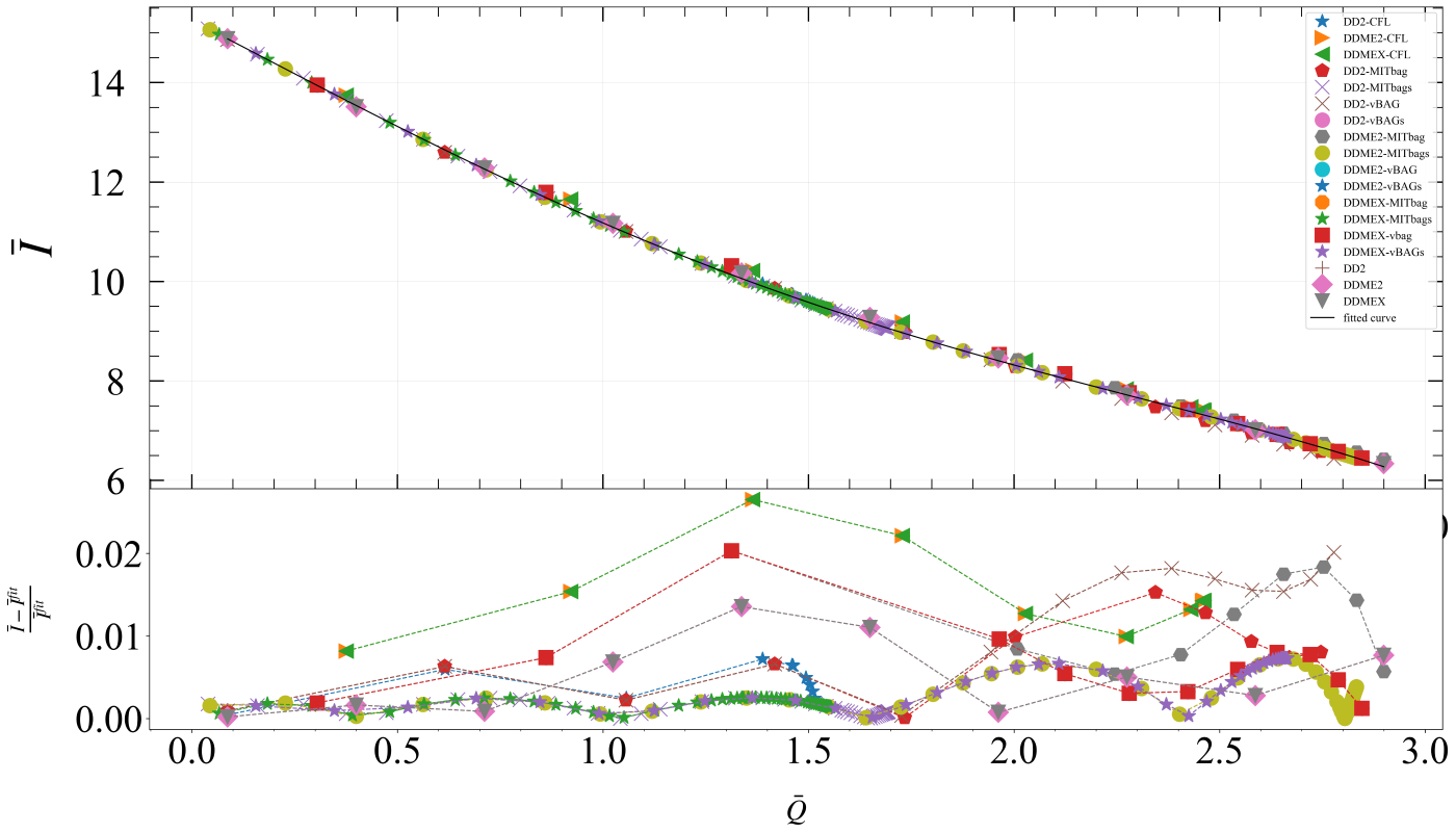
(a)

(b)

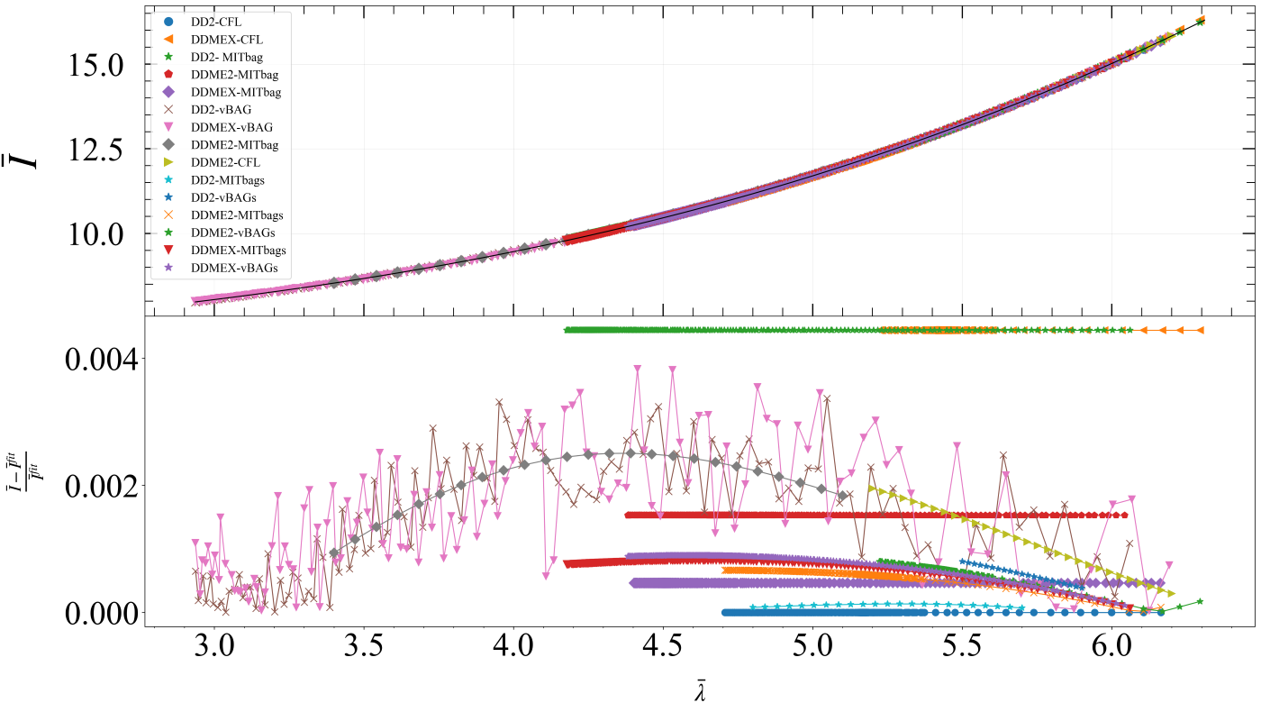
(c)

Figure 3: (a)I-Q relation along with the analytic fit and the fractional error in the moment of inertia of HSs from the fitting function is shown. The value of $\chi^{2}=1.383\times 10^{-3}$. (b) $Q-\lambda$ relation along with the analytic fit and the fractional error in the moment of inertia of HSs from the fitting function is shown. The value of $\chi^{2}=2.4\times 10^{-3}$. (c) $I-\lambda$ relation along with the analytic fit and the fractional error in the moment of inertia of HSs from the fitting function is shown. The value of $\chi^{2}=3.41\times 10^{-5}$. The nomenclature for the shape remains the same.

The plot of the dimensionless moment of inertia ($\bar{I}$) and the dimensionless quadrupole moment ($\bar{Q}$) is shown in Fig. 3(a) along with the error for $\bar{I}$ due to polynomial fitting. The graphs indicate the universality of the I-Q relationship. The error graph shows that the maximum error is below $3\%$. Among all these EOS, DDMEX-CFL shows a maximum deviation of about $2-3\%$, and DDMEX MIT bag has a minimum deviation of about $0.5\%$. One of the most notable facts is that HSs with CFL quarks matter inside the core, also following this universal relationship.

The variation of dimensionless quadrupole moment ($\bar{Q}$) with respect to dimensionless tidal love number ($\bar{\lambda}$) is shown in the Fig. 3(b). All the $\bar{Q}$ values depend on $\bar{\lambda}$ rather than properties of matter as expected in a universal relation. The maximum deviation of around $3\%$ which is for DDMEX- vBAG EOS. The minimum error in Fig. 3(b) involves EOS DDME2-vBAG. The relation between $\bar{I}$ and $\bar{\lambda}$ shows also the universality which is shown in the Fig. 3(c). DDME2-vBAG and DD2 CFL have the maximum and minimum error. This fitted curve fit seems to be the best fit for this universal relation. Furthermore, we compute $\chi^{2}$ values for each curve and all of them yield very small values which statistically validate our conclusion. The $\chi^{2}$ is defined as

$$\chi^{2}=\sum\frac{(y_{obs}-y_{expt})^{2}}{y_{expt}}$$ (33)

and computed as $\chi^{2}/(d.o.f)$, where d.o.f is defined as (number of data points - number of constants).

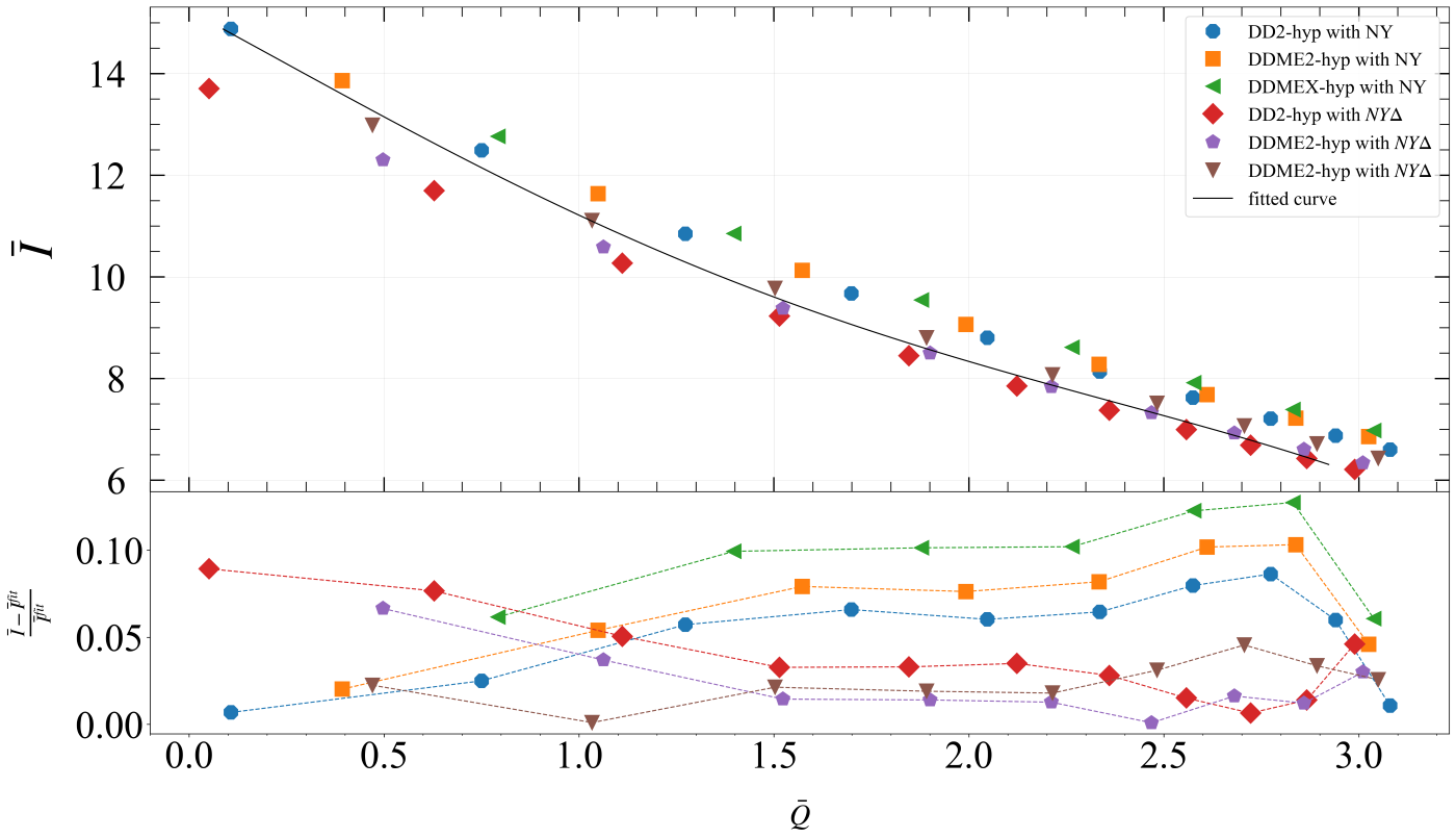
(a)

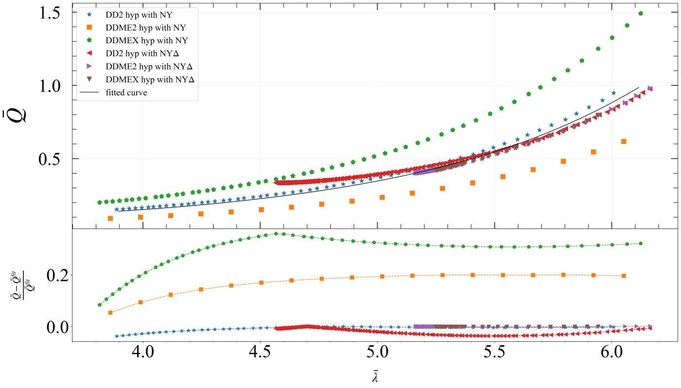
(b)

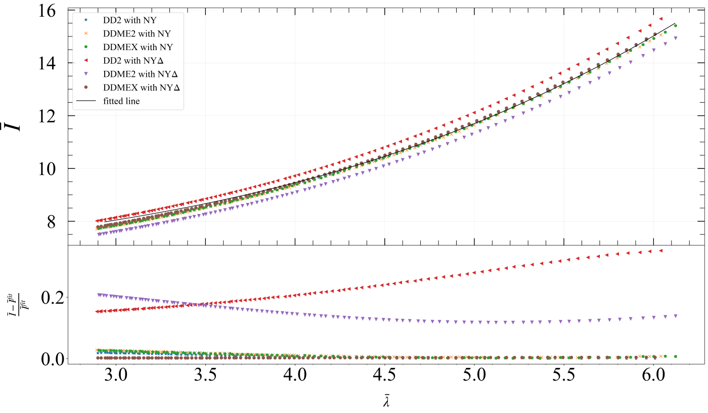
(c)

Figure 4: (a) I-Q with hyperon relation along with the analytic fit and the fractional error in the quadrupole moment of HSs from the fitting function is shown. (b) Q-$\lambda$ with hyperon relation along with the analytic fit and the fractional error in the quadrupole moment of HSs from the fitting function is shown. (c) I-$\lambda$ with hyperon relation along with the analytic fit and the fractional error in the quadrupole moment of HSs from the fitting function is shown. The nomenclature for the shape remains the same.

We plot all of the universal relations for the EOS considering the heavy baryons in Fig. 4(a), 4(b) and 4(c). On the contrary, they don’t seem to follow the universal relation like other EOSs. The error compared to the fit described earlier is very high like $20\%$. For I-Q plot DDME2 EOS with $NY\Delta$ and DDMEX with NY give maximum $15\%$ and minimum $5\%$ errors respectively. DDMEX EOS with NY and DD2 EOS with $NY\Delta$ are giving a maximum $25\%$ and minimum $5\%$ error for $Q-\lambda$ plot. For $I\lambda$, DD2 with $NY\Delta$ gives a maximum of $25\%$ and DDMEX EOS with $NY\Delta$ gives a minimum of $5\%$ of error.

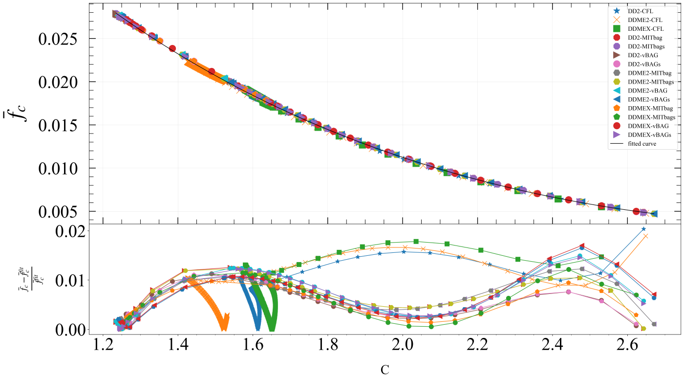
(a)

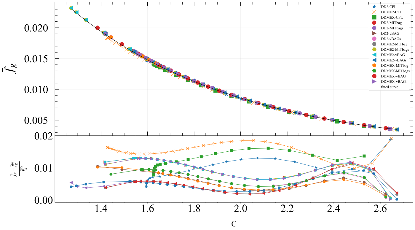
(b)

Figure 5: (a) f mode with cowling approximation vs compactness relation along with the analytic fit and the fractional error in the f mode of HSs from the fitting function is shown. The value of $\chi^{2}=4.75^{-7}$. (b) Dimensionless f-mode frequency with full GR calculations versus compactness relation along with the analytic fit and the fractional error in the f-mode of HSs from the fitting function is shown. The value of $\chi^{2}=1.165\times 10^{-6}$. The nomenclature for the shape remains the same.

Next, we plot the variation of f-mode oscillation’s frequency with respect to the compactness of the star. We use Cowling approximation and full GR to calculate the f-mode frequency in Fig. 5(a) and 5(b) respectively. In both cases, the universality is maintained very strictly, with an error under $2\%$. Note that the HSs with CFL quark matter are no exception to the universality. In the case of cowling approximation, f-modes with DD2-CFL and DD2-vBAGs show a maximum error of about $2\%$ and minimum error of about $1\%$ respectively. The same in the case of full GR calculation of f-mode is DDME2-CFL and DDMEX MITbags.

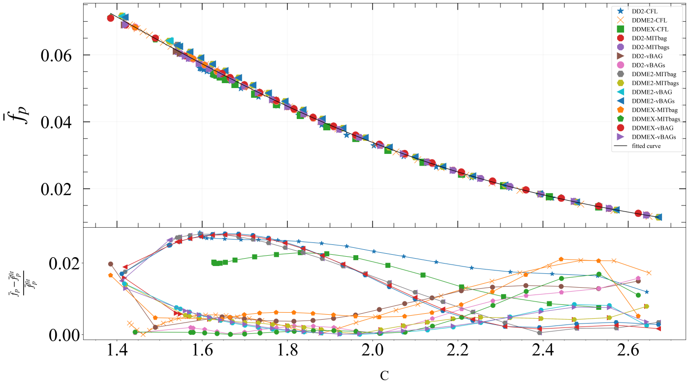
Figure 6: Frequency of p-mode vs compactness relation along with the analytic fit and the fractional error in the p-mode of HSs from the fitting function is shown. The nomenclature for the shape remains the same. The value of $\chi^{2}=1.035\times 10^{-5}$

Next, we represent the universality of p-mode oscillation frequency with the Cowling approximation in Fig. 6. Here, the maximum deviation of about $2.75\%$ with DDME2-MITbag. But here DDMEX-vBAG shows a minimum deviation of about $1.2\%$.Logarithmic fitting of the universal relation with a polynomial is advantageous. Then, by measuring one of them, it is possible to approximate the values of the other parameters without explicitly measuring them.

$y_{i}$	$x_{i}$	$a_{i}$	$b_{i}$	$c_{i}$	$d_{i}$	$e_{i}$
$\bar{I}$	$\bar{Q}$	15.254	-4.281	-0.205	0.516	-0.105
$\bar{Q}$	$\bar{\lambda}$	5.214	-4.756	1.656	-0.26	0.015
$\bar{I}$	$\bar{\lambda}$	5.135	1.53	-0.445	$9.467\times 10^{-2}$	$-2.879\times 10^{-3}$
$\bar{f}_{c}$	C	$9.446\times 10^{-2}$	$-8.424\times 10^{-2}$	$3.119\times 10^{-2}$	$-6\times 10^{-3}$	$5.348\times 10^{-4}$
$\bar{f}_{g}$	C	$11.932\times 10^{-2}$	$-14.135\times 10^{-2}$	$7.128\times 10^{-2}$	$-1.769\times 10^{-2}$	$1.774\times 10^{-3}$
$\bar{f}_{p}$	C	$11.818\times 10^{-2}$	$7.454\times 10^{-2}$	$-13.905\times 10^{-2}$	$5.327\times 10^{-2}$	$-6.462\times 10^{-3}$

Table 2: Estimated numerical coefficients for the fitting formulas.

Denoting the polynomial approximation is the

$$y_{i}=a_{i}+b_{i}(ln(x_{i}))+c_{i}(ln(x_{i}))^{2}+d_{i}(ln(x_{i}))^{3}+e_{i}(ln(x_{i}))^{4}.$$ (34)

The coefficients are given in the Table 2.

5 Conclusions and summary

The CS born after the supernova explosion contains matter at density a few times $n_{0}$. At that high density, the matter properties are not well constrained from experimental as well as theoretical points of view. Consequently, the matter at high density is modeled for different compositions and interactions between constituent particles. The macroscopic properties of CS are highly sensitive to highly dense matter models. However, a few relations between some macroscopic quantities are independent of microscopic models of highly dense matter. This was first pointed out by Yagi and Yunes in 2013 [1, 2] and supported by many consecutive studies [26, 31, 27, 28, 29, 30, 20, 21, 22, 23, 24, 25, 33, 32, 34, 35, 37, 38, 39, 40]. Most of the studies of universal relations have been done with stars composed of pure nucleonic matter - the neutron star. Other possible configurations of compact stars are baryonic stars with heavier baryons in the inner part of the star and the HS. The universal relation with HS configuration has also been studied in refs. [21, 39] with Maxwell construction of phase transition to SQM in normal phase. In this current work, we examine the universal relation for HS with Gibbs construction to SQM in the CFL phase and we find that this kind of HS also maintains the same universality with the HS having SQM in the normal phase. Then we find the universal relations between the frequencies of non-radial modes f-mode and p-mode and the compactness of the star with HS configuration. Here we have calculated the f-mode frequencies both with Cowling approximation and full relativistic treatment. The results of both treatments obey the universal relation with the compactness of stars. However, unfortunately, we find that universality fails for baryonic stars with heavier baryons inside the core of the star. This must have some implications.

Data Availability

The data used in the manuscript can be obtained at reasonable request from the corresponding author.

References

- [1] Kent Yagi and Nicolás Yunes. I-Love-Q: Unexpected Universal Relations for Neutron Stars and Quark Stars. Science, 341(6144):365–368, July 2013.
- [2] Kent Yagi and Nicolás Yunes. I-Love-Q relations in neutron stars and their applications to astrophysics, gravitational waves, and fundamental physics. Phys. Rev. D, 88(2):023009, July 2013.
- [3] Kostas D. Kokkotas and Bernd G. Schmidt. Quasi-Normal Modes of Stars and Black Holes. Living Reviews in Relativity, 2(1):2, September 1999.
- [4] Lee Lindblom and Steven L Detweiler. The quadrupole oscillations of neutron stars. Astrophysical Journal Supplement Series (ISSN 0067-0049), vol. 53, Sept. 1983, p. 73-92., 53:73–92, 1983.
- [5] Steven Detweiler and Lee Lindblom. On the nonradial pulsations of general relativistic stellar models. The Astrophysical Journal, 292:12–15, 1985.
- [6] John P. Cox. Nonradial Oscillations of Stars: Theories and Observations. Annual Review of Astronomy and Astrophysics, 14(1):247–273, September 1976.
- [7] M C Rodriguez, Ignacio F Ranea-Sandoval, C Chirenti, and D Radice. Three approaches for the classification of protoneutron star oscillation modes. Monthly Notices of the Royal Astronomical Society, page stad1459, May 2023.
- [8] K. D. Kokkotas, T. A. Apostolatos, and N. Andersson. The inverse problem for pulsating neutron stars: a ‘fingerprint analysis’ for the supranuclear equation of state. Mon. Not. Roy. Astron. Soc., 320(3):307–315, January 2001.
- [9] Nikolaos Stergioulas, Andreas Bauswein, Kimon Zagkouris, and Hans-Thomas Janka. Gravitational waves and non-axisymmetric oscillation modes in mergers of compact object binaries. Mon. Not. Roy. Astron. Soc., 418(1):427–436, November 2011.
- [10] Stamatis Vretinaris, Nikolaos Stergioulas, and Andreas Bauswein. Empirical relations for gravitational-wave asteroseismology of binary neutron star mergers. Phys. Rev. D, 101(8):084039, April 2020.
- [11] Cecilia Chirenti, Roman Gold, and M. Coleman Miller. Gravitational Waves from F-modes Excited by the Inspiral of Highly Eccentric Neutron Star Binaries. Astro. Phys. J. , 837(1):67, March 2017.
- [12] Jan Steinhoff, Tanja Hinderer, Tim Dietrich, and Francois Foucart. Spin effects on neutron star fundamental-mode dynamical tides: Phenomenology and comparison to numerical simulations. Physical Review Research, 3(3):033129, August 2021.
- [13] Athul Kunjipurayil, Tianqi Zhao, Bharat Kumar, Bijay K. Agrawal, and Madappa Prakash. Impact of the equation of state on f - and p - mode oscillations of neutron stars. Phys. Rev. D, 106(6):063005, September 2022.
- [14] Tianqi Zhao and James M. Lattimer. Universal relations for neutron star f-mode and g-mode oscillations. Physical Review D, 106(12):123002, December 2022.
- [15] Nicholas Lozano, Vinh Tran, and Prashanth Jaikumar. Temperature Effects on Core g-Modes of Neutron Stars. Galaxies, 10(4):79, June 2022.
- [16] Vivek Baruah Thapa, Mikhail V. Beznogov, Adriana R. Raduta, and Pratik Thakur. Frequencies of - and -oscillation modes in cold and hot compact stars. Phys. Rev. D, 107:103054, May 2023.
- [17] Nils Andersson and Kostas D. Kokkotas. Towards gravitational wave asteroseismology. Mon. Not. Roy. Astron. Soc., 299(4):1059–1068, October 1998.
- [18] Omar Benhar, Valeria Ferrari, and Leonardo Gualtieri. Gravitational wave asteroseismology reexamined. Phys. Rev. D, 70(12):124015, December 2004.
- [19] Cecilia Chirenti, Gibran H. de Souza, and Wolfgang Kastaun. Fundamental oscillation modes of neutron stars: Validity of universal relations. Phys. Rev. D, 91(4):044034, February 2015.
- [20] Kent Yagi and Nicolás Yunes. Binary Love relations. Classical and Quantum Gravity, 33(13):13LT01, July 2016.
- [21] Vasileios Paschalidis, Kent Yagi, David Alvarez-Castillo, David B. Blaschke, and Armen Sedrakian. Implications from GW170817 and I-Love-Q relations for relativistic hybrid stars. Phys. Rev. D, 97(8):084038, April 2018.
- [22] Hector O. Silva and Nicolás Yunes. I-Love-Q to the extreme. Classical and Quantum Gravity, 35(1):015005, January 2018.
- [23] Jérémie Gagnon-Bischoff, Stephen R. Green, Philippe Landry, and Néstor Ortiz. Extended I-Love relations for slowly rotating neutron stars. Phys. Rev. D, 97(6):064042, March 2018.
- [24] Miguel Marques, Micaela Oertel, Matthias Hempel, and Jérôme Novak. New temperature dependent hyperonic equation of state: Application to rotating neutron star models and I -Q relations. Phys. Rev. C, 96(4):045806, October 2017.
- [25] J. B. Wei, A. Figura, G. F. Burgio, H. Chen, and H. J. Schulze. Neutron star universal relations with microscopic equations of state. Journal of Physics G Nuclear Physics, 46(3):034001, March 2019.
- [26] Andrea Maselli, Vitor Cardoso, Valeria Ferrari, Leonardo Gualtieri, and Paolo Pani. Equation-of-state-independent relations in neutron stars. Phys. Rev. D, 88(2):023007, July 2013.
- [27] Michi Bauböck, Emanuele Berti, Dimitrios Psaltis, and Feryal Özel. Relations between Neutron-star Parameters in the Hartle-Thorne Approximation. Astro. Phys. J. , 777(1):68, November 2013.
- [28] B. Haskell, R. Ciolfi, F. Pannarale, and L. Rezzolla. On the universality of I-Love-Q relations in magnetized neutron stars. Mon. Not. Roy. Astron. Soc., 438(1):L71–L75, February 2014.
- [29] George Pappas and Theocharis A. Apostolatos. Effectively Universal Behavior of Rotating Neutron Stars in General Relativity Makes Them Even Simpler than Their Newtonian Counterparts. Phys. Rev. Lett., 112(12):121101, March 2014.
- [30] Kent Yagi, Koutarou Kyutoku, George Pappas, Nicolás Yunes, and Theocharis A. Apostolatos. Effective no-hair relations for neutron stars and quark stars: Relativistic results. Phys. Rev. D, 89(12):124013, June 2014.
- [31] Sayan Chakrabarti, Térence Delsate, Norman Gürlebeck, and Jan Steinhoff. I-Q Relation for Rapidly Rotating Neutron Stars. Phys. Rev. Lett., 112(20):201102, May 2014.
- [32] J. R. Stone, V. Dexheimer, P. A. M. Guichon, A. W. Thomas, and S. Typel. Equation of state of hot dense hyperonic matter in the Quark-Meson-Coupling (QMC-A) model. Mon. Not. Roy. Astron. Soc., 502(3):3476–3490, April 2021.
- [33] R. Riahi, S. Z. Kalantari, and J. A. Rueda. Universal relations for the Keplerian sequence of rotating neutron stars. Phys. Rev. D, 99(4):043004, February 2019.
- [34] Nan Jiang and Kent Yagi. Analytic I-Love-C relations for realistic neutron stars. Phys. Rev. D, 101(12):124006, June 2020.
- [35] Adriana R. Raduta, Micaela Oertel, and Armen Sedrakian. Proto-neutron stars with heavy baryons and universal relations. Mon. Not. Roy. Astron. Soc., 499(1):914–931, November 2020.
- [36] P. S. Koliogiannis and Ch. C. Moustakidis. Effects of the equation of state on the bulk properties of maximally rotating neutron stars. Phys. Rev. C, 101(1):015805, January 2020.
- [37] Daniel A. Godzieba, Rossella Gamba, David Radice, and Sebastiano Bernuzzi. Updated universal relations for tidal deformabilities of neutron stars from phenomenological equations of state. Phys. Rev. D, 103(6):063036, March 2021.
- [38] Vsevolod Nedora, Sebastiano Bernuzzi, David Radice, Boris Daszuta, Andrea Endrizzi, Albino Perego, Aviral Prakash, Mohammadtaher Safarzadeh, Federico Schianchi, and Domenico Logoteta. Numerical Relativity Simulations of the Neutron Star Merger GW170817: Long-term Remnant Evolutions, Winds, Remnant Disks, and Nucleosynthesis. Astro. Phys. J. , 906(2):98, January 2021.
- [39] Noshad Khosravi Largani, Tobias Fischer, Armen Sedrakian, Mateusz Cierniak, David E. Alvarez-Castillo, and David B. Blaschke. Universal relations for rapidly rotating cold and hot hybrid stars. Mon. Not. Roy. Astron. Soc., 515(3):3539–3554, September 2022.
- [40] Tianqi Zhao and James M. Lattimer. Universal relations for neutron star f -mode and g -mode oscillations. Phys. Rev. D, 106(12):123002, December 2022.
- [41] Daniela D. Doneva, Stoytcho S. Yazadjiev, Nikolaos Stergioulas, and Kostas D. Kokkotas. Breakdown of I-Love-Q Universality in Rapidly Rotating Relativistic Stars. Astro. Phys. J. Lett., 781(1):L6, January 2014.
- [42] George Pappas and Theocharis A. Apostolatos. Effectively universal behavior of rotating neutron stars in general relativity makes them even simpler than their newtonian counterparts. Physical Review Letters, 112(12), mar 2014.
- [43] N. K. Glendenning and S. A. Moszkowski. Reconciliation of neutron-star masses and binding of the Lambda in hypernuclei. Phys. Rev. Lett., 67:2414–1417, October 1991.
- [44] Giuseppe Colucci and Armen Sedrakian. Equation of state of hypernuclear matter: Impact of hyperon-scalar-meson couplings. Phys. Rev. C, 87(5):055806, May 2013.
- [45] M. Oertel, C. Providência, F. Gulminelli, and Ad R. Raduta. Hyperons in neutron star matter within relativistic mean-field models. Journal of Physics G Nuclear Physics, 42(7):075202, July 2015.
- [46] Adriana R. Raduta, Armen Sedrakian, and Fridolin Weber. Cooling of hypernuclear compact stars. Mon. Not. Roy. Astron. Soc., 475(4):4347–4356, April 2018.
- [47] Jia Jie Li, Wen Hui Long, and Armen Sedrakian. Hypernuclear stars from relativistic Hartree-Fock density functional theory. European Physical Journal A, 54(8):133, August 2018.
- [48] Luiz L. Lopes and Débora P. Menezes. Broken SU(6) symmetry and massive hybrid stars. Nucl. Phys. A, 1009:122171, May 2021.
- [49] Alessandro Drago, Andrea Lavagno, Giuseppe Pagliara, and Daniele Pigato. Early appearance of isobars in neutron stars. Phys. Rev. C, 90(6):065809, December 2014.
- [50] Bao-Jun Cai, Farrukh J. Fattoyev, Bao-An Li, and William G. Newton. Critical density and impact of (1232 ) resonance formation in neutron stars. Phys. Rev. C, 92(1):015802, July 2015.
- [51] Jia Jie Li, Armen Sedrakian, and Fridolin Weber. Competition between delta isobars and hyperons and properties of compact stars. Physics Letters B, 783:234–240, August 2018.
- [52] Jia Jie Li and Armen Sedrakian. Implications from GW170817 for -isobar Admixed Hypernuclear Compact Stars. Astro. Phys. J. Lett., 874(2):L22, April 2019.
- [53] Jia Jie Li, Armen Sedrakian, and Mark Alford. Relativistic Hybrid Stars with Sequential First-order Phase Transitions in Light of Multimessenger Constraints. Astro. Phys. J. , 944(2):206, February 2023.
- [54] Vivek Baruah Thapa, Monika Sinha, Jia-Jie Li, and Armen Sedrakian. Equation of state of strongly magnetized matter with hyperons and -resonances. arXiv e-prints, page arXiv:2010.00981, October 2020.
- [55] Vivek Baruah Thapa, Anil Kumar, and Monika Sinha. Baryonic dense matter in view of gravitational-wave observations. Mon. Not. Roy. Astron. Soc., 507(2):2991–3004, October 2021.
- [56] Massimo Mannarelli. Meson Condensation. Particles, 2(3):411–443, September 2019.
- [57] P. Haensel and M. Proszynski. Pion condensation in cold dense matter and neutron stars. Astro. Phys. J. , 258:306–320, July 1982.
- [58] Norman K. Glendenning and Jürgen Schaffner-Bielich. First order kaon condensate. Phys. Rev. C, 60(2):025803, August 1999.
- [59] Sarmistha Banik and Debades Bandyopadhyay. Antikaon condensation and the metastability of protoneutron stars. Phys. Rev. C, 63(3):035802, March 2001.
- [60] Vivek Baruah Thapa and Monika Sinha. Dense matter equation of state of a massive neutron star with antikaon condensation. Phys. Rev. D, 102(12):123007, December 2020.
- [61] Vivek Baruah Thapa, Monika Sinha, Jia Jie Li, and Armen Sedrakian. Massive -resonance admixed hypernuclear stars with anti-kaon condensations. arXiv e-prints, page arXiv:2102.08787, February 2021.
- [62] Z. F. Seidov. The Stability of a Star with a Phase Change in General Relativity Theory. Soviet Astronomy, 15:347, October 1971.
- [63] Edward Witten. Cosmic separation of phases. Phys. Rev. D, 30:272–285, Jul 1984.
- [64] Anil Kumar, Vivek Baruah Thapa, and Monika Sinha. Compact star merger events with stars composed of interacting strange quark matter. Mon. Not. Roy. Astron. Soc., 513(3):3788–3797, July 2022.
- [65] John C Collins and Malcolm J Perry. Superdense matter: neutrons or asymptotically free quarks? Physical Review Letters, 34(21):1353, 1975.
- [66] N. K. Glendenning. Compact Stars. Springer-Verlag New York, 1997.
- [67] Rana Nandi and Prasanta Char. Hybrid Stars in the Light of GW170817. Astro. Phys. J. , 857(1):12, April 2018.
- [68] R. O. Gomes, P. Char, and S. Schramm. Constraining Strangeness in Dense Matter with GW170817. Astro. Phys. J. , 877(2):139, June 2019.
- [69] Mauro Mariani, Milva G. Orsaria, Ignacio F. Ranea-Sandoval, and Germán Lugones. Magnetized hybrid stars: effects of slow and rapid phase transitions at the quark-hadron interface. Mon. Not. Roy. Astron. Soc., 489(3):4261–4277, November 2019.
- [70] Ishfaq A. Rather, Usuf Rahaman, M. Imran, H. C. Das, A. A. Usmani, and S. K. Patra. Rotating neutron stars with quark cores. Phys. Rev. C, 103(5):055814, May 2021.
- [71] Anil Kumar, Vivek Baruah Thapa, and Monika Sinha. Hybrid stars are compatible with recent astrophysical observations. Phys. Rev. D, 107(6):063024, March 2023.
- [72] Mark G. Alford, Andreas Schmitt, Krishna Rajagopal, and Thomas Schäfer. Color superconductivity in dense quark matter. Reviews of Modern Physics, 80(4):1455–1515, October 2008.
- [73] F. Weber. Strange quark matter and compact stars. Progress in Particle and Nuclear Physics, 54(1):193–288, March 2005.
- [74] Andrew W. Steiner, Sanjay Reddy, and Madappa Prakash. Color-neutral superconducting quark matter. Phys. Rev. D, 66(9):094007, November 2002.
- [75] Jurgen Schaffner, Carl B. Dover, Avraham Gal, Carsten Greiner, D. John Millener, and Horst Stoecker. Multiply strange nuclear systems. Annals Phys., 235:35–76, 1994.
- [76] A. Gal, E. V. Hungerford, and D. J. Millener. Strangeness in nuclear physics. Rev. Mod. Phys., 88:035004, Aug 2016.
- [77] A Feliciello and T Nagae. Experimental review of hypernuclear physics: recent achievements and future perspectives. Reports on Progress in Physics, 78(9):096301, aug 2015.
- [78] R. O. Gomes, V. Dexheimer, S. Schramm, and C. A. Z. Vasconcellos. Many-body Forces in the Equation of State of Hyperonic Matter. Astro. Phys. J. , 808(1):8, July 2015.
- [79] L. Tolos and L. Fabbietti. Strangeness in nuclei and neutron stars. Progress in Particle and Nuclear Physics, 112:103770, May 2020.
- [80] M. D. Cozma and M. B. Tsang. In-medium (1232 ) potential, pion production in heavy-ion collisions and the symmetry energy. European Physical Journal A, 57(11):309, November 2021.
- [81] Roger W. Romani, D. Kandel, Alexei V. Filippenko, Thomas G. Brink, and WeiKang Zheng. PSR J0952-0607: The Fastest and Heaviest Known Galactic Neutron Star. Astro. Phys. J. Lett., 934(2):L17, August 2022.
- [82] M. C. Miller, F. K. Lamb, A. J. Dittmann, S. Bogdanov, Z. Arzoumanian, K. C. Gendreau, S. Guillot, A. K. Harding, W. C. G. Ho, J. M. Lattimer, R. M. Ludlam, S. Mahmoodifar, S. M. Morsink, P. S. Ray, T. E. Strohmayer, K. S. Wood, T. Enoto, R. Foster, T. Okajima, G. Prigozhin, and Y. Soong. PSR J0030+0451 Mass and Radius from NICER Data and Implications for the Properties of Neutron Star Matter. Astro. Phys. J. Lett., 887(1):L24, December 2019.
- [83] M. C. Miller, F. K. Lamb, A. J. Dittmann, S. Bogdanov, Z. Arzoumanian, K. C. Gendreau, S. Guillot, W. C. G. Ho, J. M. Lattimer, M. Loewenstein, S. M. Morsink, P. S. Ray, M. T. Wolff, C. L. Baker, T. Cazeau, S. Manthripragada, C. B. Markwardt, T. Okajima, S. Pollard, I. Cognard, H. T. Cromartie, E. Fonseca, L. Guillemot, M. Kerr, A. Parthasarathy, T. T. Pennucci, S. Ransom, and I. Stairs. The Radius of PSR J0740+6620 from NICER and XMM-Newton Data. Astro. Phys. J. Lett., 918(2):L28, September 2021.
- [84] G. Lugones and J. E. Horvath. High-density QCD pairing in compact star structure. Astron. Astrophys., 403:173–178, May 2003.
- [85] Debashree Sen and Gargi Chaudhuri. Rotating hybrid stars with color-flavor-locked quark matter. Journal of Physics G Nuclear Physics, 49(7):075201, July 2022.
- [86] L. S. Rocha, A. Bernardo, M. G. B. de Avellar, and J. E. Horvath. Exact solutions for compact stars with CFL quark matter. International Journal of Modern Physics D, 29(7):2050044, January 2020.
- [87] Luiz L Lopes, Carline Biesdorf, and Débora P Menezes. Modified mit bag models—part i: Thermodynamic consistency, stability windows and symmetry group. Physica Scripta, 96(6):065303, 2021.
- [88] B. Franzon, R. O. Gomes, and S. Schramm. Effects of the quark-hadron phase transition on highly magnetized neutron stars. Mon. Not. Roy. Astron. Soc., 463(1):571–579, November 2016.
- [89] Edward Farhi and R. L. Jaffe. Strange matter. Phys. Rev. D, 30(11):2379–2390, December 1984.
- [90] A. Chodos, R. L. Jaffe, K. Johnson, Charles B. Thorn, and V. F. Weisskopf. A New Extended Model of Hadrons. Phys. Rev. D, 9:3471–3495, 1974.
- [91] K. Johnson. The M.I.T. Bag Model. Acta Phys. Polon. B, 6:865, 1975.
- [92] Hajime Sotani, Nobutoshi Yasutake, Toshiki Maruyama, and Toshitaka Tatsumi. Signatures of hadron-quark mixed phase in gravitational waves. Phys. Rev. D, 83(2):024014, January 2011.
- [93] Kip S. Thorne. Nonradial Pulsation of General-Relativistic Stellar Models. III. Analytic and Numerical Results for Neutron Stars. Astro. Phys. J. , 158:1, October 1969.
- [94] Subrahmanyan Chandrasekhar and Valeria Ferrari. On the non-radial oscillations of a star. Proceedings of the Royal Society of London Series A, 432(1885):247–279, February 1991.
- [95] Hajime Sotani, Kazuhiro Tominaga, and Kei-ichi Maeda. Density discontinuity of a neutron star and gravitational waves. Physical Review D, 65(2):024010, December 2001.
- [96] Jun-Li Lü and Wai-Mo Suen. Determining the long living quasi-normal modes of relativistic stars. Chinese Physics B, 20(4):040401, April 2011.
- [97] Kip S. Thorne and Alfonso Campolattaro. Non-Radial Pulsation of General-Relativistic Stellar Models. I. Analytic Analysis for L ¿= 2. Astrophysical Journal, vol. 149, p.591, September 1967.
- [98] James B. Hartle. Slowly Rotating Relativistic Stars. I. Equations of Structure. Astro. Phys. J. , 150:1005, December 1967.
- [99] George Pappas and Theocharis A. Apostolatos. Revising the Multipole Moments of Numerical Spacetimes and its Consequences. Phys. Rev. Lett., 108(23):231104, June 2012.
- [100] Nikolaos Stergioulas and John L. Friedman. Comparing Models of Rapidly Rotating Relativistic Stars Constructed by Two Numerical Methods. Astro. Phys. J. , 444:306, May 1995.
- [101] Nozawa, T., Stergioulas, N., Gourgoulhon, E., and Eriguchi, Y. Construction of highly accurate models of rotating neutron stars - comparison of three different numerical schemes. Astron. Astrophys. Suppl. Ser., 132(3):431–454, 1998.